Fractionalization and The Tragedy of Growth

Sreenath Majumder∗

Preliminary Version, March 2009

Abstract

This paper examines the effect of population diversity or fractionalization on income growth inU.S. cities. Using city level data across decades, I find population diversity has no significantimpact on income growth. This directly contradicts the conclusion of established researchesthat fractionalization causes significant negative impact on income growth of a locality. Iconsider fractionalization and public policy to be jointly determined, and use instrumentalvariables to establish the causality between fractionalization and income growth. My resultsshow that when fractionalization is assumed to be an exogenous characteristic, it does havea significant negative impact on growth. However, instrumenting fractionalization in a 2SLSframework shows no significant impact on growth.

JEL classification: O11, O51, O15, H10Keywords: Fractionalization, Public Goods, U.S. Cities.

∗Ph.D. Candidate, Department of Economics, University of Houston, Houston, TX, 77204 (e-mail: smajumd3@mail.uh.edu).Please do not cite without author’s prior permission. I thank Prof. Bent Sorensen, Prof. Steve Craig, Prof. Dietrich Vollrath, andthe Spring 2007 University of Houston Graduate Workshop for helpful comments and discussion. Any error remains mine.

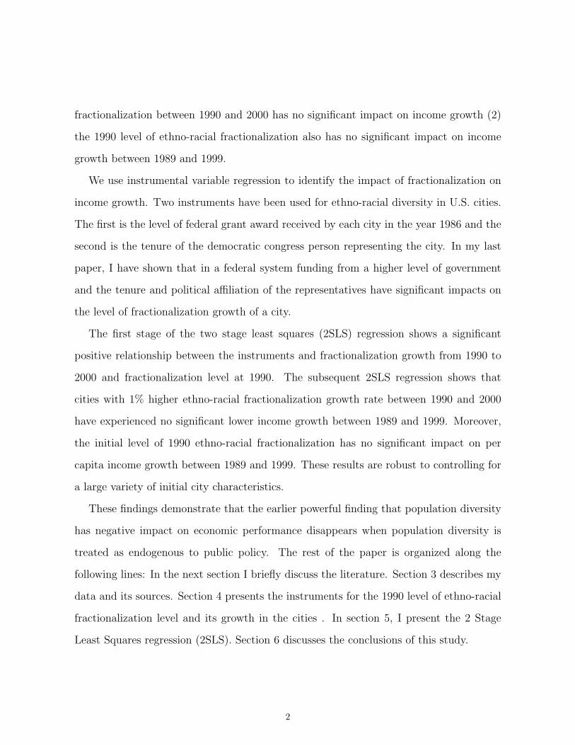
1 Introduction

Macro/growth economists try to understand the determinants of income growth of a soci-

ety from many angles. Although they have different opinions about the main determinants

of growth, most of them agree that population diversity of a society is a very significant

determinant for growth. Most of them believe that higher population diversity causes

lower economic growth. In this paper, I show that this conclusion does not hold true.

The economic logic that higher diversity/ fractionalization causes lower growth is based

on the assumption that fractionalization is a static characteristic of a society, and, hence,

it is completely exogenous to public policy design. In my previous paper, I have shown

that in a set-up where population flow is very persistent this assumption is not tenable.

Results show that public policies regarding city governmentsS expenditure on a couple of

important categories of public goods do have a very significant impact on fractionalization

growth in U.S. cities. Hence, fractionalization is not an exogenous cause of public policy

design as is assumed by the most part of the literature. Thus the question, what effect

does endogenous fractionalization have on the income growth of a locality proves to be

very interesting.

In order to answer this question we need a geographic set up where people can move

freely across localities. In a cross country setting this is hardly possible. Therefore, our

empirical analysis is based on U.S. cities, where there are few impediments to people’s

movement across cities, in terms of language, cultural differences, foods habits, social

barriers, transportation cost, and political boundaries. There exists a wide variation of

ethno-racial diversity across U.S. cities. As a result, they offer a unique opportunity to

examine the impact of fractionalization on income growth.

Using the census data of twelve ethno-racial groups of 819 cities for two census years,

our results show that fractionalization has no significant impact on income growth when it

is treated as endogenous. We have two main empirical results - (1) growth of ethno-racial

1

fractionalization between 1990 and 2000 has no significant impact on income growth (2)

the 1990 level of ethno-racial fractionalization also has no significant impact on income

growth between 1989 and 1999.

We use instrumental variable regression to identify the impact of fractionalization on

income growth. Two instruments have been used for ethno-racial diversity in U.S. cities.

The first is the level of federal grant award received by each city in the year 1986 and the

second is the tenure of the democratic congress person representing the city. In my last

paper, I have shown that in a federal system funding from a higher level of government

and the tenure and political affiliation of the representatives have significant impacts on

the level of fractionalization growth of a city.

The first stage of the two stage least squares (2SLS) regression shows a significant

positive relationship between the instruments and fractionalization growth from 1990 to

2000 and fractionalization level at 1990. The subsequent 2SLS regression shows that

cities with 1% higher ethno-racial fractionalization growth rate between 1990 and 2000

have experienced no significant lower income growth between 1989 and 1999. Moreover,

the initial level of 1990 ethno-racial fractionalization has no significant impact on per

capita income growth between 1989 and 1999. These results are robust to controlling for

a large variety of initial city characteristics.

These findings demonstrate that the earlier powerful finding that population diversity

has negative impact on economic performance disappears when population diversity is

treated as endogenous to public policy. The rest of the paper is organized along the

following lines: In the next section I briefly discuss the literature. Section 3 describes my

data and its sources. Section 4 presents the instruments for the 1990 level of ethno-racial

fractionalization level and its growth in the cities . In section 5, I present the 2 Stage

Least Squares regression (2SLS). Section 6 discusses the conclusions of this study.

2

2 Literature Review

Fractionalization or population diversity is measured from different angels such as eth-

nic origin, racial identity, language spoken, religious affiliation etc. An index called the

Harfindhal index is been used to represent fractionalization. This index is constructed

using total population shares of different population groups in a locality. The index has

an intuitive construction and interpretation. It has been included in the famous World

Handbook of Political and Social Indicators by Taylor and Hudson.

Fractionalization or population diversity has become a “standard” explanatory variable

in cross country growth regressions after the influential articale published by Easterly

and Levine (1997). 1 In this paper they have shown, in a cross country settings, higher

ethnolinguistic fractionalization has a strong negative impact on per capita GDP growth

of a country. They argued it is the higher ethnolinguistic diversity among the population

of African countries that are responsible for their miserable growth tragedy. A large part

of the macro growth literature broadly confirms their results. Works such as La Porta

et al. (1999), Alesina, Baquir, and Easterly (1999), Katz (1999), Annett (2001), Alesina

and La Ferrara (2002), Caselli and Coleman (2002), and many more fall in this category.

Alesina et al. (2003) substantially updated the original ethno-linguistic fractioanlization

index called as ELF using mainly data sourse from the Encyclopedia Britannica for 190

counties in the year 1990. Their comprehensive measure of fractionalization confirmed the

earlier findings that there exists a robust negative causal relationship between ELF and

growth. They found higher ethnic diversity is associated with low government quality.4

The literature on fractionalization, that find diversity has a negative outcome on eco-

nomic performance of a locality, based upon the assumption that higher population het-

erogeneity within a society is reflected in higher fractionalization of preference for public

policies among the population. This creates interest conflicts among populations within1The general Growth empirics exercises of Doppelhofer et al. (2000), Brock and Durlauf (2001).4For overviews of the literature on effect of fractionalization on public policies, see Alesina and La Ferrara (2003)[pp. 14]

3

that society. A particular public policy is preferred by some groups but not preferred by

others. The interest conflicts make it harder for the society to have a consensus regarding

its present and future goals, and the policy design to achieve those goals. The result is

poor and inefficient public policies that ultimately lead to suboptimal economic perfor-

mance of the society. The assumption of exogenous fractionalization, however, contradicts

their basic argument that different racial or ethnic groups have different preference struc-

tures concerning public policies. Because in that case any public policy would differently

affect different ethnic or racial group populations. This will induce different ethnic or

racial groups to sort themselves among localities whose public policies fit their preference

the best. This sorting of population among localities along the line of race and ethnic-

ity would necessarily change the fractionalization of the localities. Therefore considering

this interdependency between fractionalization and public policy is more logical way to

measure the impact of fractionalization on economic growth.

3 Data, Source, and Descriptive Statistics

I analyze the per capita income growth rate in U.S. cities where the population in 1980,

1990, and 2000 were 25,000 or more. The index I use to calculate ethno-racial fraction-

alization (ethnic) measures the probability that two people drawn randomly from a city

will belong to two different ethno-racial groups. The construction of ethnic is as follows:

ethnic = 1−n∑

i=1

(Si)2 (1)

0 ≤ ethnic ≤ 1

Where Si is the population share of ith race in a city and n is the total number of

ethno-racial groups in a city.

I have all together 12 ethno-racial population categories for each of my two sample

years, 1990 and 2000. Therefore i = Non-Hispanic White, Non-Hispanic Black, Non-

Hispanic American Indians and Alaskan Native, Non-Hispanic Asian, Non-Hispanic Pa-

4

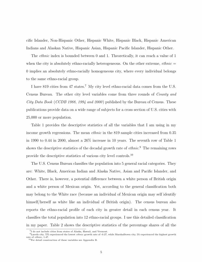
cific Islander, Non-Hispanic Other, Hispanic White, Hispanic Black, Hispanic American

Indians and Alaskan Native, Hispanic Asian, Hispanic Pacific Islander, Hispanic Other.

The ethnic index is bounded between 0 and 1. Theoretically, it can reach a value of 1

when the city is absolutely ethno-racially heterogeneous. On the other extreme, ethnic =

0 implies an absolutely ethno-racially homogeneous city, where every individual belongs

to the same ethno-racial group.

I have 819 cities from 47 states.7 My city level ethno-racial data comes from the U.S.

Census Bureau. The other city level variables come from three rounds of County and

City Data Book (CCDB 1988, 1994 and 2000 ) published by the Bureau of Census. These

publications provide data on a wide range of subjects for a cross section of U.S. cities with

25,000 or more population.

Table 1 provides the descriptive statistics of all the variables that I am using in my

income growth regressions. The mean ethnic in the 819 sample cities increased from 0.35

in 1990 to 0.44 in 2000, almost a 26% increase in 10 years. The seventh row of Table 1

shows the descriptive statistics of the decadal growth rate of ethnic.9 The remaining rows

provide the descriptive statistics of various city level controls.10

The U.S. Census Bureau classifies the population into 5 general racial categories. They

are: White, Black, American Indian and Alaska Native, Asian and Pacific Islander, and

Other. There is, however, a potential difference between a white person of British origin

and a white person of Mexican origin. Yet, according to the general classification both

may belong to the White race (because an individual of Mexican origin may self identify

himself/herself as white like an individual of British origin). The census bureau also

reports the ethno-racial profile of each city in greater detail in each census year. It

classifies the total population into 12 ethno-racial groups. I use this detailed classification

in my paper. Table 2 shows the descriptive statistics of the percentage shares of all the7I do not include cities from states of Alaska, Hawaii, and Vermont.9Laredo city, TX experienced the lowest ethnic growth rate of -0.27, while Marshalltown city, IA experienced the highest growth

rate of ethnic, 1.47.10For detail construction of these variables see Appendix B.

5

12 groups for the 820 sample cities in 1990 and 2000.

Table 3 shows the various ranges of the decadal growth rate of ethnic in my 820

sample cities. It shows that in 5.5% of my sample cities the decadal growth rate of ethnic

is negative. In around 14% cities the growth rate lies between 0% to 10%. In 58% cities

the growth rate is in between 10% and 50%. In 22% cities the growth rate is in between

50% and 100%. In around 1% cities the decadal growth rate of ethnic is more than 100%.

It is clear from Table 2 that fractionalization is not a static characteristic of U.S. cities.

Moreover, there is a wide variation across cities in terms of its growth rate. A deeper

investigation is required to understand the reason for this wide variation.

4 Instruments for Public Goods Spending

4.1 Tenure

There is a strong possibility that in a democratic system as the one prevailing in the

United States the power of fund allocation for a locality is related to the tenure of its

representative and his/her political affiliation. Therefore, the tenure of the representative

of a city and his/her political affiliation can potentially serve as instruments for city

governments’ public goods expenditure.

I take the total tenure and the political affiliation of the congressperson from a city as

an instrument for city governments’ expenditure on public goods.11 Instrumenting a city

government’s public goods expenditure in 1990 with the tenure of the congress person

who represented that city up to 1990, involves three distinct steps. In step one, I have to

find out the number of that corresponding congressional district (CD) to which the city

belongs.12 Then I have to find out the name of the congress person who served that CD11The United States is divided into several congressional districts (CDs); each of these is an electoral constituency that elects

a single member to represent in one of the two chambers of the U.S. Congress – the House of Representatives. The length of aterm in the U.S. House of Representatives is two years. Therefore a congress person has a lifespan of two years in the House ofRepresentatives for each term.

12CDs are represented with a number along with the name of the state to which they belong. For example 11th district ofAlabama means the 11th CD of Alabama

6

up to 1990. In the third step, I have to calculate his/her total tenure in the U.S. House

of Representatives up to 1990, and find out to which political party he/she belonged.13

In doing so there are some potential problems. First, many of my cities belong to

multiple CDs and, hence, I cannot map a city with a corresponding CD uniquely. Second,

the boundaries of the CDs can change in every census. Thus, city A may belong to the

11th CD of Texas in 1990 but could have been in the 1st CD of Texas in 1979. In order

to solve the first problem and to uniquely map a city to its corresponding CD in 1990, I

select the CD whose representative congress person had the highest tenure in the House

of Representatives.14 In case of the second problem, I take the 100th congress (with term

from 1987 to 1989) as the relevant congress with its districts’ boundaries to map my

sample cities with their corresponding CDs.15

Following these rules, I uniquely map each of my 820 sample cities with its correspond-

ing congressional district, and calculate the total tenure of the representative congress

person from the cities in the House of Representatives up to the year 1989. Then I con-

struct a variable indicating the total tenure of the congress person from Democratic Party.

The reason I chose to focus on the tenure of Congress persons from the Democratic Party

is that starting from 1955 to 1995 i.e. from the 84th to the 103rd congress, all the con-

gresses were Democrat majority congresses. Hence, I can assume that being members of

the Democratic Party in Democrat majority congresses, these congress persons acquired

sufficient power to allocate funds to their districts and, by extension, to their cities.16

13For example, I want to instrument 1990’s public goods expenditure of City A in Texas. First, I have to find out the districtnumber to which city A belongs to in 1990. Let us say it belongs to the 3rd district of Texas. Then I have to find out who wasthe congress person in 3rd CD of Texas in 1990. Say it was congress person i. Then I have to find out the total number of yearscongress person i served in the House of Representatives, i.e. his/her total tenure in the House of Representatives up to the year1990, and his/her political affiliation.

14In order to calculate tenure of the congress person, I take into account the total number of years he/she has served in the Houseof Representatives throughout his/her congressional career up to 1989.

15The boundaries of the CDs of the 100th congress were set up in the 1980 census (i.e. in the middle of the 96th congress).Therefore, even if the district number and boundary of a CD changed in the 1980 census a congress person who got elected in the96th congress and got subsequent re-elections up to the 100th congress served his/her district at least for 9 years. I think that is asufficient time to attach a congressman to his/her CDs and city.

16Out of my 820 sample cities in 1990, 285 cities had a Democratic congress person with a total tenure of 10 years or more.

7

4.2 Federal Grants

Financial assistance to a lower level of government from a higher level can be an influential

factor for the lower level government’s expenditure level. In the federal system of the

United States the local governments like city, county, or state governments receive financial

assistance from the federal government. I use the variation in federal assistance as an

instrument for city governments’ expenditure on public services. The instrument is the

per capita federal grant award received by each city in the year 1986. There are 15

categories of federal assistances available to states and their subdivisions. Of these seven

are financial types of assistance and eight are non-financial types of assistance. The grant

award includes two types of grants, the formula grants and the project grants.17 Table 1

shows the descriptive statistics of grants, the per capita federal grant awards received by

the cities in the year 1986.

5 Income Growth in U.S. Cities – 2SLS Regressions

5.1 The Determinants of City’s fractionalization level

The second stage of my 2SLS regression, which I measure to identify the impact of frac-

tionalization on per capita income growth is :

ln(PCI1999)i − ln(PCI1989)i = α + β ln(ethnic1990)i + γ ln(X)i + εi (2)

ln(PCI1999)i − ln(PCI1989)i measures the growth rate of per capita income in city i

between 1999 and 1989. ln(ethnic1990)i is the ethno-racial fractionalization level in city

i in 1990. Xi is the vector of other city level characteristics in 1990 or prior to that

and εi is a random error term. The coefficient of interest is β, the effect of ethno-racial

fractionalization on income growth.17For detail see Catalog of Federal Domestic Assistance. The data on federal grant awards used in my research is taken from the

1988 County and City Data Book.

8

Since I believe that income and population heterogeneity are not exogenous causes

to each other, I consider cities’ ethno-racial diversity (ethnic) as an endogenous vari-

able. Therefore, I instrument it with my two instruments grant and tenure. Equation

(3) describes the relationship between cities’ ethno-racial fravtionalization level and its

determinants, including my two instruments. Therefore, equation (3) represents the first

stage regression:

ln(ethnic1990)i = αg + βg ln(grant)i + γg(tenure)i + δg ln(X)i + νgi (3)

where ln(grant)i is the log amount of the per capita grant awards received by the ith

city in 1986, and tenurei is the dummy variable for ith city showing whether in 1989

the congress person representing the city had an experience of 10 years or more in the

House of Representatives, and if he/she was from the Democratic Party. Panel B of Table

4 shows results of the first stage regression. The coefficient βg and γg are positive and

statistically significant in both specifications. The large F statistics in both specifications

shows that the my instruments are strong.18

5.2 Income Growth and Level of Fractionalization

The first and third columns of panel A in Table 4 reports the ordinary least squares (OLS)

regression results of per capita income growth on level of fractionalization. Column one

shows that cities in 1990 with 1% higher ethno-racial population diversity experienced a

0.2% lower growth of per capita income between 1989 and 1999. After controlling for all

city level characteristics plus 50 state dummies, the impact of fractionalization level on

income growth is still robust and significant as exhibited in column two. Cities in 1990 with

higher ethno-racial population diversity experienced a significant lower income growth.

This result is consistent with the established literature that assumes fractionalization as18which jointly test the hypothesis that the coefficients of the two excluded instruments grant and tenure in the first stage equals

zero.

9

an exogenous characteristics of a locality.

But as we argued previously fractionalization is not an exogenous cause of public policy

and hence to income. Considering the level of ethno-racial fractionalization in equation (2)

as endogenous and modeling it with equation (3) gives the IV regression results in column

three and four. The result of column three shows no negative impact of fractionalization

on income growth. Cities with higher fractionalization in 1990 actually experienced a

higher income growth. After including all of my city level controls plus state fixed effects

the result of column four shows no significant relationship between population diversity

and income growth. For the validity of the two instruments, grant and tenure must not

affect the dependent variable (i.e. the growth of ethnic) directly, but only through public

goods spending. I test this over identification restriction with the standard Hansen J

test. The null hypothesis of this test is that the instruments are uncorrelated with the

IV regression residuals. The large p-values of the Hansen J-statistics reported in the

second and the fourth column of Table 4 show that we can accept the null and, hence,

the instruments pass the test in both specifications.

The IV estimates of Table 4 show that considering population diversity as endogenous

characteristics of locality, determined by public policy, shows diversity does not cause lower

income growth. Thus the earlier findings that population diversity causes poor economic

performance of a society seems to be originates from the strong assumption that diversity

is a static factor and hence completely exogenous to any public policy design.

5.3 Income Growth and Growth of Fractionalization

Another interesting angel to analyze the impact of population diversity on economic per-

formance of a locality is to measure the causal impact of fractionalization growth on

income growth. In my earlier paper I have shown ethno-racial diversity in U.S. cities are

not a static factor. As a result regressing the growth of per capita income on the growth

of ethno-racial diversity can give us more logical impact. To measure this impact the base

10

line regression that I measure is

ln(PCI1999)i − ln(PCI1989)i = α + β[∆(ethnic)i] + γ ln(X)i + εi (4)

Where [∆(ethnic)i] is ln(ethnic2000)i− ln(ethnic1990)i, the growth rate of ethno-racial frac-

tionalization in city i between 1990 and 2000.

Again as previous fractionalization growth is treated as endogenous and instrumented

with per capita federal grant received by the cities in 1986, ln(grant)i and tenure of the

democratic congress person from the city, ln(tenure)i.

ln(ethnic2000)i − ln(ethnic1990)i = αg + βg ln(grant)i + γg(tenure)i + δg ln(X)i + νgi (5)

Panel A of table 5 reports the IV regression results. Column I shows the impact of

fractionalization growth on income growth in 819 U.S. cities with out any controls. Result

shows cities with 1% higher growth rate of ethno-racial fractionalization between 1990 to

2000, experienced a 9% significant lower per capita income growth between 1989 to 1999.

However after controlling for other city level characteristics, this effect tend to disappear.

Cities with 1% higher fractionalization growth does not have any significant impact on

income growth.

6 Conclusion

Population diversity as measured by ethnic origin as well as racial identity has no sig-

nificant impact on income growth in U.S. cities. This result critically depends upon the

finding that fractionalization is not a static exogenous characteristics. The result here

clearly indicate that economic growth is hardly depends upon population diversity when

population is mobile. It is the public policy design that has the ultimate say to shape

the economic performance of a society. It is now interesting to examine this question in

11

a cross-country setting where established literature has an unambiguous finding, higher

fractionalization causes lower growth.

12

References

Acemoglu, D., S. Johnson, and J. A. Robinson, “The Colonial Origins of Comparative De-

velopment: An Empirical Investigation,” American Economic Review, XCI (2001),

1369-1401.

Alesina, A., A. Devleeschauwer, W. Easterly, S. Kurlat, and R. Wacziarg, “Fractionalization,”

Journal of Economic Growth, VIII (2003), 155-194.

Alesina, A., E. Glaeser, and B. Sacerdote, “Why Doesn’t the US Have a European-Style

Welfare State?” Brookings Papers on Economic Activity, MMI (2001), 187-254.

Alesina, A., and E. Zhuravskaya, “Segregation and the Quality of Government in A Cross-

Section of Countries,” NBER Working Paper No. 14316, 2008.

Alesina, A., and E. L. Ferrara, “Ethnic Diversity and Economic Performance,”Journal of

Economic Literature, XLIII (2005), 721-761.

Alesina, A., and E. Spolaore, “On the Number and Size of Nations,”Quarterly Journal of

Economics, CXII (1997), 1027-1056.

Alesina, A., E. Spolaore, and R. Wacziarg, “Economic Integration and Political Disinte-

gration,” American Economic Review, XC (2000), 1276-1296.

Alesina, A., R. Baqir, and C. Hoxby, “Political Jurisdictions in Heterogeneous Communi-

ties,” Journal of Political Economy, CXII (2004), 348-396.

Alesina, A., R. Baqir, and W. Easterly, “Public Goods and Ethnic Divisions,” Quarterly

Journal of Economics, CXIV (1999), 1243-1284.

Alesina, A., R. Baqir, and W. Easterly, “Redistributive Public Employment,” Journal of

Urban Economics, XLVIII (2000), 219-241.

Banerjee, A., and R. Somanathan, “Caste, Community and Collective Action: The Polit-

ical Economy of Public Good Provision in India,” unpublished, 2001.

Barrow, R. J., and X. Sala-i-Martin, “Convergence,”Journal of Political Economy, C (1992),

223-251.

Barrow, R. J., and X. Sala-i-Martin, Economic Growth (Cambridge, MA: MIT Press, 2003).

Bell, Derrick, Faces at the Bottom of the Well: The Permanence of Racism (New York:

Basic Books, 1992).

13

Borjas, G. J., Economics of Migration (St. Louis, MO: Elsevier, 2000).

Borjas, G. J., “Immigration and Welfare Magnets,” Journal of Labor Economics, XVII

(1999), 607-637.

Campos, N. F., and V. S. Kuzeyev, “On the Dynamics of Ethnic Fractionalization,”Amer-

ican Journal of Political Science, LI (2007), 620-639.

Caselli, F., and W. J. Coleman II, “On the Theory of Ethnic Conflict,” NBER Working

Paper No. 12125, 2006.

Easterly, W., and R. Levine, “Africa’s Growth Tragedy: Policies and Ethnic Divisions,”

Quarterly Journal of Economics, CXII (1997), 1203-1250.

Epple, D., and T. Romer, “Mobility and Redistribution,” Journal of Political Economy,

XCIX (1991), 828-858.

Goldin, C., and L. Katz, “Human Capital and Social Capital: The Rise of Secondary

School in America, 1910 to 1940,”Journal of Interdisciplinary History, XXIX (1999),

683-723.

Hacker, Andrew, Two Nations: Black and White, Separate, Hostile and Unequal (New

York: Scribner’s, 1995).

Huckfeldt, R., and C. W. Kohfeld, Race and the Decline of Class in American Politics

(Urbana: University of Illinois Press, 1989).

Kaestner, R., N. Kaushal, and G. V. Ryzin, “Migration Consequences of Welfare Reform,”

NBER Working Paper No. 8560, 2001.

Kozol, J., Savage Inequalities: Children in America’s Schools (New York: Crown Pub-

lishers Inc., 1991).

La Porta, R., et al., “The Quality of Government,” Journal of Law, Economics, and Or-

ganization, XV (1999), 222-279.

Michalopoulas, S., “The Origins of Ethnolinguistic Diversity: Theory and Evidence,” un-

published, 2008.

Munshi, K., and N. Wilson, “Identity, Parochial Institutions, and Occupational Choice:

Linking the Past to the Present in the American Midwest,” NBER Working Paper

No. 13717, 2008.

Page, C., Showing My Color: Impolite Essays on Race and Identity (HarperCollins, 1996).

14

Posner, D., “The Implications of Constructivism for Studying the Relationship Between

Ethnic Diversity and Economic Growth,” in K. Chandra, ed., Ethnicity, Politics, and

Economics, Working Paper No. 13717, 2004.

Rappaport, J., “Moving to Nice Weather,”Regional Science and Urban Economics, XXXVII

(2007), 375-398.

Rappaport, J., “Why are Population Flows so Persistent?” Journal of Urban Economics,

LVI (2004), 554-580.

Rhode, P. W., and K. S. Strumpf, “Assessing the Importance of Tiebout Sorting: Local

Hetrogeneity from 1850 to 1990,” American Economic Review, XCIII (2003), 1648-

1677.

Rubinfeld, D., P. Shapiro, and J. Roberts, “Tiebout Bias and the Demand for Local Pub-

lic Schooling,” Review of Economics and Statistics, LXIX (1987), 426-437.

Sokoloff, K. L., and S. L. Engerman, “History Lessons: Institutions, Factors Endowments,

and Path of Development in the New World,”Journal of Economic Perspectives, XIV

(2000), 217-232.

Tajfel, H., M. Billig, R.P. Bundy, and C. Flament, “Social Categorization and Intergroup

Behavior,” European Journal of Social Psychology, I (1971), 149-178.

Tiebout, C., “A Pure Theory of Local Expenditures,”Journal of Political Economy, LXIV

(1956), 416-24.

Vigdor J., “Community Composition and Collective Action: Analyzing Initial mail re-

sponses to 2000 Census,” Review of Economics and Statistics, LXXXVI (2004), 303-

312.

Wilson, W., When Work Disappears: The World of the New Urban Poor (New York:

Knopf-distributed by Random House, Inc., 1996).

15

Table 1: Descriptive Statistics

Obs Mean S.D. Min Max Unitper capita income 1989 819 21.21 4.8 9.3 66 Thousand dollar per capitaper capita income 1999 819 14.53 7.1 5.8 55 Thousand dollar per capitagrowth rate of PCI 819 0.38 0.09 0.08 0.77 Fractionethnic90 819 0.35 0.20 0.03 0.79 Fractionethnic00 819 0.44 0.19 0.06 0.81 Fraction% of Graduates 1990 819 22.38 11.38 3.7 71.2 Fractionmedian rent 1990 819 475 145 239 1001 Dollarunemployment rate 1991 819 6.8 2.6 0.8 17.9 Fractionfirm establishments 1987 819 12 5.4 141 11.7 Thousand per capitatotal population 1990 819 11.4 32.7 25 7322.5 Thousandpercentage of old population 1990 819 13.12 4.79 2.7 48.5 Fractionspending 1990 819 429.0 223.6 91.2 2068.7 Dollar per capitagrant 819 283.9 972.8 2.3 137.6 Hundred dollar per capitacity Area 1990 819 39.6 69.4 1 758.7 Square Miles

Notes: ethnic90: city ethno-racial fractionalization in 1990, ethnic00: city ethno-racial fractionalization in 2000.

ethnict = 1−∑n

i=1(Si,t)2, Where Si is the population share of ith ethno-racial group in a city in year t and n is the total number of

ethno-racial groups in a city in year t, i = Non-Hisp. White, Non-Hisp. Black, Non-Hisp. American Indians and Alaskan Native,

Non-Hisp. Asian, Non-Hisp. Pacific Islander, Non-Hisp. Other, Hisp. White, Hisp. Black, Hisp. American Indians and Alaskan Native,

Hisp. Asian, Hisp. Pacific Islander, Hisp. Other. t = 1990, 2000. ethnic5races,t: city ethno-racial fractionalization in year t using 5

categories of races (White, Black, American Indian and Eskimo, or Aleut, Asian or Pacific Islander, and Other). ethnic2race,t: city

ethno-racial fractionalization in year t using 2 categories of races (non-Hispanic White and All Other). growth rate ethnic: Growth

rate of ethnic between 1990 and 2000 measured as ln(ethnic2000)− ln(ethnic1990). median rent 1990: median gross rent (for

renter-occupied housing units) in a city in 1990. unemployment rate 1991: civilian unemployed as a % of total civilian labor force in

the city in 1991. per capita income 1989: city level per capita income in 1989. firm establishments 1987:

1987 city per capita total number of (manufacturing firms establishments with 20 or more employees + wholesale trade establishments

+ retail trade establishments with payroll + taxable service establishments with payroll). total population 1990: city aggregate

population in 1990. percentage of old population: % of total city population with age more than 65 years in 1990. spending 1990: city

governments’ 1990 aggregate per capita general expenditure on welfare, health, police, highways, fire, and sewerage and solid

waste management. grant: amount of per capita federal grant awards received by cities in 1986. city area 1990: total city land area

in 1990.

16

Table 2: Ethno-racial Group’s Population Shares in U.S. Cities − Descriptive Statistics

2000 1990Obs Mean S.D. Min Max Obs Mean S.D. Min Max Unit

non Hisp. white 819 65.30 22.62 1.02 97.09 820 73.89 20.63 1.46 98.68 %non Hisp. black 819 14.14 16.85 0.13 88.23 820 12.71 15.75 0.05 88.51 %non Hisp. aian 819 0.52 1.11 0.02 16.45 820 0.51 1.00 0.02 13.10 %non Hisp. asian 819 4.27 6.74 0.11 61.47 820 3.13 5.00 0.03 56.01 %non Hisp. pi 819 0.11 4.22 0.00 2.78 820 0.03 0.12 0 1.94 %non Hisp. other 819 2.09 1.20 0.16 14.41 820 0.13 0.25 0 4.73 %Hisp. white 819 6.38 8.93 0.07 79.94 820 4.99 8.29 0.12 79.00 %Hisp. black 819 0.28 0.39 0 3.60 820 0.30 0.55 0 5.87 %Hisp. aian 819 0.15 0.19 0 1.25 820 0.07 0.09 0 0.71 %Hisp. asian 819 0.05 0.06 0 0.58 820 0.05 0.11 0 1.35 %Hisp. pi 819 0.02 0.02 0 0.16 820 0.07 0.15 0 1.33 %Hisp. other 819 6.68 8.80 0.06 55.62 820 4.10 6.94 0.03 64.98 %

Notes: City level observations for the year 1990 and 2000.

non Hisp. white: non-Hispanic White, non Hisp. black: non-Hispanic Black

non Hisp. aian: non-Hispanic American Indian; Eskimo; or Aleut.

non Hisp. asian: non-Hispanic Asian, non Hisp. pi: non-Hispanic Pacific Islander.

non Hisp. other: non-Hispanic Other, Hisp. white: Hispanic White, Hisp. Black: Hispanic black

Hisp. aian: Hispanic American Indian; Eskimo; or Aleut.

Hisp. asian: Hispanic Asian, Hisp. pi: Hispanic Pacific Islander, Hisp. other: Hispanic Other.

Table 3: Ranges of ethnic Change in U.S. Cities

Growth Rate of ethnic Number of Cities % of Total CitiesNegative 45 5.49More than 0% but less than 10% 112 13.66More than 10% but less than 50% 475 57.93More than 50% but less than 100% 179 21.83More than 100% 9 1.10

Notes: ethnic: ethno-racial fractionalization level in a city, calculated using 12 ethno-racial population

categories.

Growth rate of ethnic measure the decadal growth rate of ethnic from 1990 to 2000 and calculated as

ln(ethnic2000)− ln(ethnic1990).

17

Table 4: Growth of Income in U.S. CitiesPanel A: IV Estimates

Dep. Var: ln(PCI 1999) - ln(PCI 1989) (OLS) (OLS) (IV) (IV)

ln ELF 1990 -0.02*** -0.03*** 0.04*** 0.01(0.00) (0.00) (0.01) (0.02)

ln % of Graduate pop 1990 0.06*** 0.04***(0.01) (0.01)

ln Median Rent 1990 -0.07** -0.10***(0.03) (0.03)

ln PC Firm Establishments 1987 -0.01 -0.02(0.01) (0.01)

ln Unemployment Rate 1990 0.02 0.00(0.01) (0.02)

ln Percentage of old population 1990 -0.01 0.02(0.01) (0.01)

ln City Area 1990 0.00 -0.00(0.00) (0.00)

ln PCI 1989 -0.02 0.03(0.03) (0.04)

State Dummies Yes Yes Yes YesR2 0.30 0.35 0.18 0.30Hansen J Statistic (p value) 0.64 0.16

Panel B: First Stage for ln ELF 1990Dep. Var: ln ELF 1990ln grant 0.15*** 0.13***

(0.01) (0.02)ln tenure 0.04** 0.03**

(0.02) (0.01)F-test of excluded instruments 70.96 39.09Number of observations 819 819 819 819

Notes: Robust standard errors are in parentheses. ***significant at 1%, **significant at 5%, *significant at 10%.

Instrumenting ELF 1990 with grant 1986 and tenure

18

Table 5: Growth of Income in U.S. CitiesPanel A: IV Estimates

Dep. Var: ln(PCI 1999) - ln(PCI 1989) (I) (II)

ln (ELF 2000) - ln (ELF 1990) -0.09*** -0.04(0.00) (0.06)

ln % of Graduate pop 1990 0.04**(0.02)

ln Median Rent 1990 -0.09***(0.03)

ln PC Firm Establishments 1987 -0.02(0.01)

ln Unemployment Rate 1990 0.00(0.02)

ln Percentage of old population 1990 -0.02(0.01)

ln City Area 1990 0.00(0.00)

ln PCI 1989 0.03(0.04)

State Dummies Yes YesR2 0.26 0.32Hansen J Statistic (p value) 0.64 0.17

Panel B: First Stage for Growth rate of ELF 1990Dep. Var: ln (ELF 2000) - ln (ELF 1990)ln grant -0.06*** -0.04***

(0.01) (0.01)ln tenure -0.02*** -0.01**

(0.01) (0.01)F-test of excluded instruments 71.53 28.23Number of observations 819 819

Notes: Robust standard errors are in parentheses. ***significant at 1%, **significant at 5%, *significant at 10%.

Instrumenting ln (ELF 2000) - ln (ELF 1990) with grant 1986 and tenure

19

Appendix

Data and Variable Construction

Ethno-racial Fractionalization Index:

ethnic = 1−n∑

i=1

(Si)2 (6)

Where Si is the population share of ith race in a city and n is the total number of

ethno-racial groups in a city (n=12).

Total population in city j in year t = Total population of (non-Hispanic White + non-

Hispanic Black + non-Hispanic American Indians and Alaskan Native + non-Hispanic

Asian + non-Hispanic Pacific Islander + non-Hispanic Other + Hispanic White + Hispanic

Black + Hispanic American Indians and Alaskan Native + Hispanic Asian + Hispanic

Pacific Islander + Hispanic Other) in city j in year t, t = 1990, 2000. (Source: U.S.

Census Bureau.)

ethnic index for 5 ethno-racial groups is calculated using the same formula (equation

(17))where the names of the ethno-racial groups are White, Black, American Indian and

Eskimo or Aleut, Asian or Pacific Islander, and Other. In this case total population in

city j in year t = Total population number of (White + Black + American Indian and

Eskimo or Aleut + Asian or Pacific Islander + Other) in city j in year t, t = 1990, 2000.

(Source: County and City Data Book 1990 )

ethnic index for 2 ethno-racial groups is calculated using the same formula (equation

(17)) where the names of the ethno-racial groups are non-Hispanic White, and All Other.

In this case total population in city j in year t = Total population number of (non-Hispanic

White + All Other) in city j in year t, t = 1990, 2000. (Source: U.S. Census Bureau.)

ethnic index for 1980 is calculated using the same formula and using the population

shares of 5 ethno-racial groups - white, black, American Indian and Eskimo and Aleut,

Asian and Pacific islander, and other. (Source: County and City Data Book 1988 )

Growth rate of ethnic is calculated as ln(ethnic2000) - ln(ethnic1990).

Median Rent

Median rent for the year 1990 gives the dollar value of median gross rent for specified

renter occupied housing paying cash rent in 1990. (Source: County and City Data Book

1990 )

20

Unemployment Rate

1991 civilian unemployment in a city as a percent of total civilian labor force in that city.

(Source: County and City Data Book 1990 )

Per Capita Income

1989 and 1999 dollar amount of per capita money income of the resident of a city based

on resident population enumerated as of April 1, 1990 and April 1, 2000. (Source: U.S.

Census Bureau.)

Firm Establishments

This is calculated as follows:

Total number of firm establishments in 1987 = Total number of Manufacturing estab-

lishments with employees in 1987 + Total number of Wholesale establishments in 1987

+ Total number of Retail trade establishments with payroll in 1987 + Total number of

taxable Service industries with payroll in 1987.

Total number of Manufacturing establishments with employees in 1987 = Total Man-

ufacturing establishments in 1987 × % of Manufacturing establishments with 20 or more

employees in 1987.

Then per capita firm establishments in a city in 1987 = Total number of firm estab-

lishments in 1987 / Total city population in 1986. (Source: County and City Data Book

1990 )

Total City Population

1990 aggregate city population. (Source: County and City Data Book 1990 )

6.0.1 Old Population

% of 1990 total city population with age between 65 to 74 years + % of 1990 total city

population with age between 75 years and over. (Source: County and City Data Book

1990 )

Federal Grant

This represents the dollar amount of Federal Grant awards to the cities in 1986.

1986 per capita grant to a city = The dollar amount of Federal Grant awards to the

city in 1986/ Total city population in 1986. (Source: County and City Data Book 1988 )

21

City Area

Total 1990 square miles of dry land (and partially covered by water) area of city. (Source:

County and City Data Book 1990 )

22