FPGA Design of an Intra 16 × 16 Module for …file.scirp.org/pdf/CS20100100003_76647181.pdf ·...

Circuits and Systems, 2010, 1, 18-29 doi:10.4236/cs.2010.11004 Published Online July 2010 (http://www.SciRP.org/journal/cs)

Copyright © 2010 SciRes. CS

FPGA Design of an Intra 16 × 16 Module for H.264/AVC Video Encoder

Hassen Loukil1, Imen Werda1, Nouri Masmoudi1, Ahmed Ben Atitallah2, Patrice Kadionik3 1University of Sfax, National School of Engineering, Sfax, Tunisia

2University of Sfax, High Institute of Electronics and Communication, Sfax, Tunisia 3IMS laboratory-ENSEIRB-MATMECA-University Bordeaux 1-CNRS UMR 5218, 351 Cours de la Libération, Talence

Cedex, France E-mail: [email protected]

Received May 16, 2010; revised June 18, 2010; accepted June 23, 2010

Abstract In this paper, we propose novel hardware architecture for intra 16 × 16 module for the macroblock engine of a new video coding standard H.264. To reduce the cycle of intra prediction 16 × 16, transform/quantization, and inverse quantization/inverse transform of H.264, an advanced method for different operation is proposed. This architecture can process one macroblock in 208 cycles for all cases of macroblock type by processing 4 × 4 Hadamard transform and quantization during 16 × 16 prediction. This module was designed using VHDL Hardware Description Language (HDL) and works with a 160 MHz frequency using ALTERA NIOS-II de-velopment board with Stratix II EP2S60F1020C3 FPGA. The system also includes software running on an NIOS-II processor in order to implementing the pre-processing and the post-processing functions. Finally, the execution time of our HW solution is decreased by 26% when compared with the previous work. Keywords: Nios H.264, FPGA, Intra 16 × 16, NIOS-II, SOPC Design

1. Introduction Currently, video system development is generally based on embedded systems. Such systems need to find a com- promise between computational complexity and timing execution constraints. On the other hand, the H.264/AVC standard for video compression [1-5], due to its high complexity, needed powerful processors and hardware acceleration in order to respect application requirements.

In order to take advantages of hardware acceleration, each functional module of the H.264 video encoder has been carefully studied in order to determine its computational complexity. Furthermore, the intra process presents one of the highest computational complexities in H.264/AVC encoder [6]. This process is based on the hybrid encoding scheme shown in Figure 1 which uses the intra prediction, integer cosine transform and quantization. The intra process is used to remove spatial redun- dancy. There are two types of intra modes: intra 4 × 4

Current Frame (Fn)

Reconstructed FrameF(n)

Intra Prediction

+

-

+

+

Transform Quantization CAVLC

Inverse Transform

Inverse Quantization

Deblocking Filter

Figure 1. Hybrid encoder for video compression.

H. LOUKIL ET AL.


19 and intra 16 × 16 modes. The intra 16 × 16 is composed of intra 16 × 16 prediction (IP 16 × 16), integer cosine transform (ICT), quantization AC (QAC), inverse integer cosine transform (IICT), inverse quantization AC (IQ- AC), quantization DC (QDC), Hadamard transform (HT), inverse quantization DC (IQDC) and inverse Hadamard transform (IHT). Special hardware implementations of intra 16 × 16 for H.264 have been proposed [7,8]. They were shown that some of these parts can be optimized with parallel hardware structures implemented into the hardware system. These previous works have implemented the intra 16 × 16 algorithm with serial [7] and parallel [8] architectures directly into hardware device. But, our architecture uses both a parallel and pipelined structures in order to reduce the number of operations and the abil-ity to achieve fast execution. Our design is described with VHDL (VHSIC Hardware Description Language) language and has been synthetized with the Altera NIOS II softcore processor for experimental validation into a single Altera Stratix II EP2S60 FPGA (Field Program-mable Gate Array) device.

This paper is organized as follows: Section 2 presents an overview of intra 16 × 16 algorithm. In the next Sec- tion, we present the intra 16 × 16 architecture. The exp- eriment results are shown in Section 4. Finally, Section 5 concludes the paper. 2. Overview of the Intra 16 × 16 Algorithm The intra 16 × 16 algorithm is a critical component used in the H.264/AVC. There are eleven functional operations in this module: intra 16 × 16 prediction, residual calculation, integer transform, AC coefficient quantization, DC coefficient quantization, inverse AC coefficient quantization, inverse DC coefficient quantization, Hada- mard transform, inverse Hadamard transform, inverse integer transform and pixel reconstruction. The 16 × 16 intra prediction mode is designed according to directions: vertical, horizontal, DC and plane modes are specified in the H.264 standard based on the reconstituted pixels from the previous macroblock (MB). Figure 2 shows the intra 16 × 16 prediction mode.

For each MB, we compute the difference between the predicted pixel and the original pixel. After this step, we calculate the integer transform coefficients. In the H.264/ AVC standard, the equation of the 4 × 4 integer transform is defined by [3,4].

1221

1111

2112

1111

I ×

1121

2111

2111

1121

XXXX

XXXX

XXXX

XXXX

15141312

111098

7654

3210

(1)

“Xi” is the residual 4 × 4 block. After this operation, we obtain two coefficients types:

AC and DC coefficients. For the AC coefficients, we compute the quantization operation. In general the AC quantization operation is defined by [3,4].

)QStep

PFIround(Z ijij (2)

We can write (5) as follows:

)2qbits

MFIround(Z ijij (3)

where:

Qstep

PFqbits2

MF (4)

qbits = 15 + floor(QP/6) (5)

Iij is the uncalled coefficients after ICT for QAC. PF represents the scaling factor of the integer transform and QStep is the quantization step size. A total of 52 values of QStep are supported by the standard as shown in Tab- le 1 where QStep doubles in size for every 6 values of the step of quantization QP.

V …………… .

Mode 0 (vertical)

V

… … … … ..

Mode 1 (horizontal)

VMean (H+V)

Mode 2 (DC)

V

Mode 3( plane)

H H

H H

Figure 2. 16 × 16 intra prediction mode.

H. LOUKIL ET AL.


20

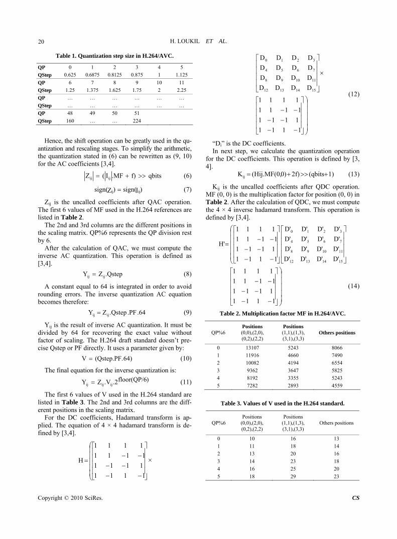
Table 1. Quantization step size in H.264/AVC.

QP 0 1 2 3 4 5

QStep 0.625 0.6875 0.8125 0.875 1 1.125

QP 6 7 8 9 10 11

QStep 1.25 1.375 1.625 1.75 2 2.25

QP … … … … … …

QStep … … … … … …

QP 48 49 50 51

QStep 160 … … 224

Hence, the shift operation can be greatly used in the qu-

antization and rescaling stages. To simplify the arithmetic, the quantization stated in (6) can be rewritten as (9, 10) for the AC coefficients [3,4].

qbitsf).MFI(Z ijij (6)

)Isign()Zsign( ijij (7)

Zij is the uncalled coefficients after QAC operation. The first 6 values of MF used in the H.264 references are listed in Table 2.

The 2nd and 3rd columns are the different positions in the scaling matrix. QP%6 represents the QP division rest by 6.

After the calculation of QAC, we must compute the inverse AC quantization. This operation is defined as [3,4].

.QstepZY ijij (8)

A constant equal to 64 is integrated in order to avoid rounding errors. The inverse quantization AC equation becomes therefore:

.64 .PF .QstepZY ijij (9)

Yij is the result of inverse AC quantization. It must be divided by 64 for recovering the exact value without factor of scaling. The H.264 draft standard doesn’t pre- cise Qstep or PF directly. It uses a parameter given by:

64)(Qstep.PF.V (10)

The final equation for the inverse quantization is: )floor(QP/6.2.VZY ijijij (11)

The first 6 values of V used in the H.264 standard are listed in Table 3. The 2nd and 3rd columns are the different positions in the scaling matrix.

For the DC coefficients, Hadamard transform is ap-plied. The equation of 4 × 4 hadamard transform is de-fined by [3,4].

1111

1111

1111

1111

H ×

1111

1111

1111

1111

DDDD

DDDD

DDDD

DDDD

15141312

111098

7654

3210

(12)

“Di” is the DC coefficients. In next step, we calculate the quantization operation

for the DC coefficients. This operation is defined by [3, 4].

1)(qbits2f)0)(Hij.MF(0,Kij (13)

Kij is the uncalled coefficients after QDC operation. MF (0, 0) is the multiplication factor for position (0, 0) in Table 2. After the calculation of QDC, we must compute the 4 × 4 inverse hadamard transform. This operation is defined by [3,4].

15141312

111098

7654

3210

D'D'D'D'

D'D'D'D'

D'D'D'D'

D'D'D'D'

1111

1111

1111

1111

H'

1111

1111

1111

1111

(14)

Table 2. Multiplication factor MF in H.264/AVC.

QP%6 Positions (0,0),(2,0), (0,2),(2,2)

Positions (1,1),(1,3), (3,1),(3,3)

Others positions

0 13107 5243 8066

1 11916 4660 7490

2 10082 4194 6554

3 9362 3647 5825

4 8192 3355 5243

5 7282 2893 4559

Table 3. Values of V used in the H.264 standard.

QP%6 Positions

(0,0),(2,0), (0,2),(2,2)

Positions (1,1),(1,3), (3,1),(3,3)

Others positions

0 10 16 13

1 11 18 14

2 13 20 16

3 14 23 18

4 16 25 20

5 18 29 23

H. LOUKIL ET AL.


21

“D’i” is the block 4 × 4 quantified DC. The final step for the DC coefficient is the inverse DC

quantization. This operation is defined by [3,4].

ij ij

for(QP 12)

floor(QP / 6) 2W H' .V(0,0).2

(15)

ij ij

for(QP 12)

1 floor(QP / 6 )W [H' .V(0,0) 2 ] (2 floor(QP / 6 ))

where V(0,0) is the multiplication factor for position (0,0) in Table 3.

After all operations, we can combine the AC and the DC coefficients for compute the inverse integer trans-form. Equation (19) gives the equation of 4 × 4 inverse integer defined as [3,4].

1/2111

111/21

111/21

1/2111

X'X'X'X'

X'X'X'X'

X'X'X'X'

X'X'X'X'

1/2111/2

1111

11/21/21

1111

I'

15141312

111098

7654

3210

(16)

“X’i” is the block 4 × 4 after all operations (AC and DC coefficients).

3. Intra 16 × 16 Architecture The intra 16 × 16 architecture partitions the MB into sixteen 4 × 4 blocks. The scanning order for one MB is shown in Figure 3. This order is scanned in the x direc-tion first and then performs the scanning in the y direc-tion. The scanning order is the label order from top to bottom, from left to right which is the actual processing order for one MB. The MB is partitioned into sixteen 4 × 4 small sub-blocks. The partitions between the 16 × 16 scanning order labels and the 4 × 4 scanning order labels are shown in Figure 4.

The 4 × 4 scanning order labels are shown in Figure 5.

0 1 2 3

16 17 18 19

32

48

4 5 6 7

20 21 22 23

8 9 10 11

24 25 26 27

12 13 14 15

28 29 30 31

64

80

96

112

128

144

160

176

192

208

224

240 241 242 243 244 245 246 247 248 249 250 251 252 253 254 255

33 34 35 36 37 38 39 40 41 42 43 44 45 46 47

49 50 51 52 53 54 55 56 57 58 59 60 61 62 63

65 66 67 68 69 70 71 72 73 74 75 76 77 78 79

81 82 83 84 85 86 87 88 89 90 91 92 93 94 95

97 98 99 100 101 102 103 104 105 106 107 108 109 110 111

113 114 115 116 117 118 119 120 121 122 123 124 125 126 127

129 130 131 132 133 134 135 136 137 138 139 140 141 412 143

145 146 147 148 149 150 151 152 153 154 155 156 157 158 159

161 162 163 164 165 166 167 168 169 170 171 172 173 174 175

177 178 179 180 181 182 183 184 185 186 187 188 189 190 191

193 194 195 196 197 198 199 200 201 202 203 204 205 206 207

209 210 211 212 213 214 215 216 217 218 219 220 221 222 223

225 226 227 228 229 230 231 232 233 234 235 236 237 238 239

x

y

Figure 3. 16 × 16 scanning order labels.

Figure 4. Relationship between 16 × 16 and 4 × 4 scanning order labels.

H. LOUKIL ET AL.


22

0 1 2 3

4 5 6 7

8 9 10 11

12 13 14 15 Figure 5. 4 × 4 scanning order labels.

Figure 6 shows the functional flow diagram of the in-

tra 16 × 16 process. In the first step, we compute the intra prediction 16 ×

16 for all 4 × 4 blocks. After this, we calculate the residual, the integer transform, the AC quantization and the inverse AC quantization for each 4 × 4 block. During the

calculation of integer transform, we extract the DC coefficient for each 4 × 4 block. After obtain the 16 DC coefficients, we calculate the hadamard transform, the DC quantization, the inverse hadamard transform and the inverse DC quantization. Finally, we combine AC and DC coefficient for each 4 × 4 block to perform the inverse integer transform and the reconstruction pixels.

The intra 16 × 16 hardware architecture is composed by two modules. The first component contains the intra 16 × 16 prediction module and the residual module. The second component contains the coding chain module and the reconstruct module. The block diagram of the proposed hardware architecture for H.264 video coding is shown in Figure 7.

intra 16x16 prediction

Combine reconstructed coefficients

Inverse Integer transform

Reconstruct pixels

For 4x4block from 0 to 15

Wait until all 4x4 blocks were Integer transformed

Extract DC coefficients(16 coeff = one 4x4

block )

Hadamard

DC Quantization

Inverse Hadamard

Inverse DC Quantization

Calculate residual

Integer transform

AC Quantization and inverse AC

Quantization

For 4x4block from 0 to 15

Store and reorder quantized coefficients

and output them when needed

AC path DC path

4x4block = 15

Yes

No

4x4block = 15

Yes

No

Start

End

Figure 6. Intra 16 × 16 functional flow diagram.

H. LOUKIL ET AL.


23 3.1. Intra 16 × 16 Prediction

Different works have been proposed [9-13]. For our architecture, the MB pixels are loaded into a dual RAM (Random Access Memory) for reordering and then give (to the residual or reconstruction blocks) by sets of 16 pixels (4 × 4 block).

This block calculates the predicted pixels of MB for all 3 intra 16 × 16 prediction modes specified in the H.264 standard (horizontal, vertical and DC) in parallel based on the reconstituted pixels from the previous MB (planar mode is not used [14]). Figure 8 presents the

intra prediction hardware architecture. These predicted pixels are stored into RAM for all modes. We also use a SAD_ 4 × 4 block for calculating the SAD value for each mode. We accumulate this value 16 times in order to obtain the SAD_16 × 16 for each mode. Those absolute values permit to give the sum of absolute differences (SAD) for each prediction mode. The comparator compares the SAD values for all prediction modes and picks the lowest value for determining which prediction mode will be used. After obtaining the best SAD (MIN_SAD), the best MB is given. The difference between the predicted pixels and the source pixels is then calculated for the best pre-diction mode for obtain the residual MB.

Control Unit

START

Done

Intra 16x16 Prediction

SRC_0

SRC_15

.

.

.8

RECON_IN0

RECON_IN31

.

.

.16

Residual_0

Residual_15

.

.

. Coding chain

Residual_out0

Residual_out15

.

.

.

16

16

Reconstruction

RECON_OUT0

RECON_OUT15

.

.

.

8

8

Start_PRED Start_CHAIN Start_RECON

8

8

8

16

16

Pred_pixel_0

Pred_pixel_15

.

.

. Residual

Start_RES

8

8

Figure 7. Intra 16 × 16 hardware architecture.

Horizontal mode

Vertical mode

DC mode

RAM Horizontal

RAM Vertical

RAM DC

Pixels_h

128 bits

Pixels_dc

128 bits

Pixels_v

128 bits

Pixels_h

128 bits

Pixels_v

128 bits

Pixels_dc

128 bits

Horizontal SAD4x4

Vertical SAD4x4

DC SAD4x4

+

+

+

Comparator

12 bits

SAD4x4_h Hor_SAD_16x16

Ver_SAD_16x16

DC_SAD_16x16

16 bits

16 bits

16 bits

MIN_SADRECON_IN0

RECON_IN31

8 bits

8 bits

SRC_0

SRC_15

12 bits

SAD4x4_v

12 bits

SAD4x4_dc

Start_pred

Start_pred

Start_pred

Wren Rden

Wren Rden

Wren Rden

Start_sad

Start_sad

Start_sad Start_comp

Control UnitCLK

Reset

Start

Start_pred

Wren

rden

Start_sad

Start_comp

Figure 8. Intra 16 × 16 prediction hardware architecture.

H. LOUKIL ET AL.


24 3.2. ICT and HT Architectures Different works have been published on the integer transform [15-19]. It is obvious that “I” shown in (1) or “H” shown in (12) can be implemented by a 1-D transform. Figure 9 shows the fast implementation for the integer transform. The matrix contains only four coefficients: 1, –1, 2, and –2. It also can be implemented by using addi- tion, subtraction and shift operations.

The Hadamard transform matrix is very similar to the integer transform matrices. The difference is that the coefficients of Hadamard transform are only 1 or –1. There- fore, the fast implementation for the Hadamard transform is shown in Figure 10.

The hardware implementation of 1-D ICT or HT is given in Figure 11. The input for this module is a 4 × 4 block. For full transform operation, we use two 1-D transforms in order to obtain the 2-D transform. Figure 12 presents the architecture for the 2-D transform.

x0-x3x0+x3 x1+x 2 x 1-x2

< << <

y1 y3y2y0

Figure 9. Fast implementations of H.264 integer transform.

x0-x3x 0+ x3 x 1+x2 x1-x2

y1 y3y2y 0

Figure 10. Fast implementations of H.264 Hadamard transform.

ICT_0

y0

y3

y1

y2

x0

x3

x1

x2 ICT_1

y0

y3

y1

y2

x0

x3

x1

x2

ICT_2

y0

y3

y1y2

x0

x3

x1x2 ICT_3

y0

y3

y1y2

x0

x3

x1x2

3,32,31,30,3

3,22,21,20,2

3,12,11,10,1

3,02,01,00,0

xxxx

xxxx

xxxx

xxxx

3,32,31,30,3

3,22,21,20,2

3,12,11,10,1

3,02,01,00,0

yyyy

yyyy

yyyy

yyyy

3,0

2,0

1,0

0,0

x

x

x

x

3,1

2,1

1,1

0,1

x

x

x

x

3,2

2,2

1,2

0,2

x

x

x

x

3,3

2,3

1,3

0,3

x

x

x

x

0,3

0,2

0,1

0,0

y

y

y

y

1,3

1,2

1,1

1,0

y

y

y

y

2,3

2,2

2,1

2,0

y

y

y

y

3,3

3,2

3,1

3,0

y

y

y

y

1-D transform block

reset

CLK

Done

start

Figure 11. Fast implementations of H.264 1-D transform.

1-D transform

1-D transform

CONTROL

CLKresetstart

Input_0..159

output_0..159

Done

Figure 12. Fast implementations of H.264 2-D transform.

3.3. QAC & QDC Architectures The Quantization hardware architectures have been proposed in [8,20]. The architecture of DC quantization is similar to the AC quantization presented in Figure 13. The multiplication factors stated in Table 1 are stored into ROM (Read Only Memory) and selected according to the QP%6 values. The correct factor is multiplied by the uncalled coefficient in the corresponding position. The shifter will shift the product to right with qbits.

The QAC or QDC modules will quantify at the same time 16 pixels according to QP factor. These modules are composed by a quantization block (noted 0…15), a memory for storing the input pixels (noted input_0..15) and two read-only memories for storing QE (equal to QP%6) and F values noted respectively ROM_QE and ROM_F. The AC and DC quantization blocks are constituted by three basic components presented in Figure 14.

0 1 2 3

4 5 6 7

8 9 10 11

12 13 14 15

ROM_F

ROM_QE

F

QE

Input_0..15

Input_0..15

CLK

reset

start

6

qp

16 16Input_0..15 Output_0..15

Figure 13. Quantization architecture.

>> out

MF(i,j)

F

QE

input

SIGN

30

15

16

416

Figure 14. AC or DC quantification.

H. LOUKIL ET AL.


25

A multiplier deals perform the multiplication operation of AC coefficients with the corresponding MF (i, j) factor and gives the absolute value. An adder will perform the sum operation of values given by the multiplier with the F parameter given by the ROM memory. A shifter allows performing the shift operation the result from the adder by “qbits” (varies 15 to 23 according to the value of QP). 3.4. IQAC & IQDC Architectures The IQAC or IQDC modules will quantify 16 pixels according to the QP factor. The architecture of these modules is similar to the QAC or QDC modules respectively presented by the Figure 13. The difference between quantization (AC or DC) and inverse quantization (AC or DC) is presented in the quantization block. For having the inverse AC quantization values, we use a multiplier to perform the multiplication operation between the QAC coefficients and the V (i, j) values. We also use a shifter for shifting the result from the multiplier floor (QP/6). The architecture for this module is presented by the Fig- ure 15.

For the DC coefficients, we use a multiplier to perform the multiplication operation between the QDC co-efficients and the V (0, 0) value. An adder will perform the sum of values given by the multiplier with {0, 1, 2} (0 for QP > = 12, 1 for QP < 12, 2 others parts). A shifter will perform the shift of result from the adder by floor (QP/6) – 2) for QP >= 12 and by (2 – floor (QP/6)) for QP < 12. The architecture for this module is presented in Figure 16. 3.5. IICT and IHT Architectures The IICT or IHT architectures are similar to the ICT or HT architectures respectively presented by the Figures 12 and 13. The inverse integer transform matrix contains only four coefficients: 1, –1, 1/2, and –1/2. Figure 17 shows the fast implementation for the inverse integer transform. The inverse Hadamard transform matrix contains only two coefficients, 1 and –1. Figure 18 shows the fast implementation for the inverse Hadamard trans-form.

> > out

V(i ,j)

inpu t

S IG Nqp

6

23

16

6

Figure 15. AC inverse quantification.

>> out

V(0,0)

{0,1,2}

QE

input

SIGN 6

6

6

23

Figure 16. DC inverse quantification.

y0-y2y0+y2 y1+(y3>>1) (y1>>1)-y3

x3 x1 x2x0

Figure 17. Fast implementations of H.264 inverse integer transform.

y0-y 2y 0+y2 y1+y3 y1-y3

x 3x0 x 1 x2

Figure 18. Fast implementation of H.264 inverse Hadamard transform.

3.6. Intra 16 × 16 Execution Time The intra 16 × 16 execution time is presented in Figure 19. This figure is divided into two parts. The first part concerns the intra 16 × 16 prediction. This part takes 115 clock cycles for the best predicted MB [21]. The second part concerns the coding chain block that needs 77 clock cycles. In this part, we use a pipeline as shown in Figure 19. To get the reconstructed MB, we need 16 clock cy-cles. Finally, 208 clock cycles are necessary to achieve the intra 16 × 16 operations. Comparing with [7] and [8], the proposed architecture takes less clock cycles. Simu-lation of our proposed RTL design shows major im-provements by reducing clock cycles for the intra 16 × 16 operation as shown in Table 4. Thus, our hardware implementation is optimized to achieve higher perform-ances for the H.264 video encoder than the hardware architecture presented in [7-8]. 4. Experimental Results The whole design has been designed by using VHDL

H. LOUKIL ET AL.


26

(RTL level). The VHDL code of all modules was synth- esized for an EP2S60F1020C3 Altera Stratix II FPGA circuit by using the Altera Quartus tool. Table 5 shows the implementation results of the intra 16 × 16 module for the Stratix II EP2S60 FPGA circuit.

For experimental verification, we have developed a C language reference model of H.264 software. We have compared the output results of our C reference model with the JM 10.1 model [22] and we have confirmed the correctness of our model. We have also used the NIOS II softcore processor for sending data to the intra frame hardware coprocessor. The block diagram of the implemented H.264 intra frame encoder is shown in Figure 20. The design is composed by three parts: the NIOS II processor, the intra 16 × 16 frame module and the other peripherals connected to the Altera Avalon Bus. The Avalon bus has control, data and address signals and has its bus arbitra-tion logic.

Our embedded system has been tested by using the Al- tera NIOS II development board. The heart of the target board is the Altera Stratix II EP2S60F1020C3 FPGA circuit. For all experiments, CIF test sequences are coded at 30 Hz. We have focussed on the following video test sequences: “Foreman”, “Paris”, “Mobile”, “Tb420” and “Akiyo”. These test sequences have different movement and camera particularities.

We have determined the processing time of intra 16 × 16 for the SW (software) solution. From the Table 6, we can conclude that a 35 time improvement for the processing speed compared to the software solution can be obtained by using our HW implementation.

Table 4. Comparison between different intra 16 × 16 architectures.

architectures [7] [8] Proposed

architecture

Number cycles/MB 3307 269 208

Frequency (Mhz) 71 54 160

Execution time/MB(ns) 46.57 4.98 1.3

Table 5. Implementation results for Stratix II FPGA.

Used Resources

ALUTs 22,685/48,352 (47%)

Memory (KB) 27/2484 (1%)

Pins 526/719 (73%)

DSP block 124/288 (43%)

Table 6. Time comparison between SW and HW implementations.

Total time (ms) Sequence SW HW

Time Foreman 684.74 18.73

(ms) Paris 688.21 18.88

Mobile 689.40 18.72

Tb420 685.78 19.08

Akiyo 687.95 18.70

ICT 0 ICT 1 ICT 15

QAC 0 QAC 1 QAC 15

IQAC 0 IQAC 1 IQAC 15

HT QDC IHT IQDC

IICT 0 IICT 1 IICT 15

2 4 3 2 4 2 4 2

77 cycles

2 4 3 9 +( 15 x 2 ) = 39 cycles 2 x 16 = 32 cycles 5 cycles 1 cycle

FIFO

Intra prediction 16 x16 Coding chaine Reconstruction

115 cycles 77 cycles 16 cycles

Figure 19. Intra 16 × 16 execution time.

H. LOUKIL ET AL.


NIOS-II CPU

AV

AL

ON

IRQ

Timer

UART USB

RAM Interface

H.264 Encoder

FLASH, SRAM, SDRAM

Hardware part

µClinux

Software part

Figure 20. H.264 embedded system video encoder.

Table 7. PSNR comparison between SW and HW implementation.

PSNR Sequence SW HW/SW

Foreman 38.08 38.08

Paris 37.15 37.15

Mobile 36.37 36.37

Tb420 37.04 37.04

Akiyo 40.01 40.01

In order to evaluate the image quality given by this ar-

chitecture, we have used the average peak signal-to-noi- se ratio (PSNR) which is here used as a measure of obje- ctive quality. The PSNR metric as shown as in Table 7 has not detected any difference between the SW and HW solutions. Thus, the quality comparison confirms the correctness of the designed architecture.

The Figure 21 presents the original and the two reconstructed (one from SW, the other from HW) of the 10th frame of the test video sequences.

5. Conclusions

In this paper, we have described a new flexible and efficient HW architecture for H.264 video encoder. The hardware part has been implemented by using VHDL language. Comparing with [7] and [8], our proposed RTL implementation gives major improvements by reducing clock cycles for the intra 16 × 16 operation. The execution time is decreased by 26% even when compared with the best previous work for intra frame coding [8]. We have also designed an embedded system based on an Altera Stratix II FPGA platform running at 160 MHz in order to

Foreman sequence PSNR – Y = 38.08 dB PSNR – Y = 38.08 dB

Foreman Mobile PSNR – Y = 36.37 dB PSNR – Y = 36.37 dB

Paris sequence PSNR – Y = 37.15 dB PSNR – Y = 37.15 dB

H. LOUKIL ET AL.


28

Tb420 sequence PSNR – Y = 37.04 dB PSNR – Y = 37.04 dB

Akiyo sequence PSNR – Y = 40.01 dB PSNR – Y = 40.01 dB

(a) (b) (c)

Figure 21. (a) Original, (b) Reconstructed from SW and (c) Reconstructed from HW/SW of the 10th frame of the test video sequences.

evaluate the performance of our design in HW/SW code- sign context. We have shown that our HW solution impr- oves considerably the intra 16 × 16 process (35 times fa- ster) compared to an all software solution with the same image quality. 6. References [1] T. Wiegand, G. J. Sullivan, G. Bjøntegaard and A. Luthra,

“Overview of the H.264/AVC Video Coding Standard,” IEEE Transactions on Circuits and Systems for Video Technology, Vol. 13, No. 7, 2003, pp. 560-576.

[2] A. Luthra, G. J. Sullivan and T. Wiegand, “Introduction to the Special Issue on the H.264/AVC Video Coding Standard,” IEEE Transactions on Circuits and Systems for Video Technology, Vol. 13, No. 7, 2003, pp. 557-559.

[3] I. Richardson, “H.264 and MPEG-4 Video Compression,” John Wiley and Sons Ltd., Chichester, 2003.

[4] Joint Video Team (JVT) of ITU-T VCEG and ISO/IEC MPEG, “Draft ITU-T Recommendation and Final Draft International Standard of Joint Video Specification (ITU-T Rec. H.264 and ISO/IEC 14496-10 AVC),” May 2003.

[5] G. J. Sullivan and T. Wiegand, “Video Compression― from Concepts to the H.264/AVC Standard,” Proceed-ings of the IEEE, Vol. 93, No. 1, 2005, pp. 18-31.

[6] Y.-W. Huang, B.-Y. Hsieh, T.-C. Chen and L. G. Chen, “Analysis, Fast Algorithm, and VLSI Architecture De-sign for H.264/AVC Intra Frame Coder,” IEEE Transac-tions Circuit and Systems for Video Technology, Vol. 15, No. 3, 2005, pp. 378-401.

[7] İ. Hamzaoğlu, Ö. Taşdizen and E. Şahin, “An Efficient H.264 Intra Frame Coder System Design,” IEEE Trans-actions on Consumer Electronics, Vol. 54, No. 4, 2008, pp. 1903-1911.

[8] K. Suh, S. Park and H. Cho, “An Efficient Hardware Ar-chitecture of Intra Prediction and TQ/IQIT Module for H.264 Encoder,” ETRI Journal, Vol. 27, No. 5, 2005, pp. 511-524.

[9] B. Meng, O. C. Au, C.-W. Wong and H.-K. Lam, “Effi-cient Intra-Prediction Mode Selection for 4 × 4 Blocks in H.264,” Proceedings of International Conference on Multimedia and Expo, Baltimore, 2003, pp. 521-524.

[10] F. Pan, X. Lin, S. Rahardja, K. P. Lim, Z. G. Li, D. Wu and S. Wu, “Fast Mode Decision Algorithm for Intra pre-diction in H.264/AVC Video Coding,” IEEE Transac-tions on Circuits and Systems for Video Technology, Vol. 15, No. 7, 2005, pp. 813-822.

[11] B. Meng, O. C. Au, C. W. Wong and H. K. Lam, “Effi- cient Intra-Prediction Algorithm in H.264,” Proceedings of International Conference on Image Processing, Bar-celona, 2003, pp. 837-840.

[12] S. S. Chun, J.-C. Yoon and S. Sull, “Efficient Intra Pre-diction Mode Decision for H.264 Video,” Lecture Notes in Computer Science, Vol. 3767, 2005, pp. 168-178.

[13] H. Loukil, A. Ben Atitallah and N. Masmoudi, “An Effi-cient FPGA Parallel Architecture for H.264/AVC Intra Prediction Algorithm,” Proceeding of International Con-ference on Embedded Systems and Critical Applications, Gammarth, Tunisia, 2008, pp. 191-196.

[14] A. Kessentini, B. Kaanich, I. Werda, A. Samet and N. Masmoudi, “Low Complexity Intra 16 × 16 Prediction for

H. LOUKIL ET AL.


29

H.264/AVC,” Proceedings of International Conference on Embedded Systems & Critical Applications, Tunis, Tunisia, 2008, pp. 197-201.

[15] T.-C. Wang, Y.-W. Huang, H.-C. Fang and L.-G. Chen, “Parallel 4 × 4 2D Transform and Inverse Transform Ar-chitecture for MPEG-4 AVC/H.264,” Proceedings of the 2003 IEEE International Symposium on Circuits and Systems, Bangkok, 2003, pp. 800-803.

[16] L. Liu, Q. Lin, M. Rong and J. Li, “A 2-D Forward/In- verse Integer Transform Processor of H.264 Based on Highly-Parallel Architecture,” Proceedings of the 4th IEEE International Workshop on System-on-Chip for Real-Time Applications, Banff, July 19-21, 2004, pp. 158-161.

[17] K.-H. Chen, J.-I. Guo and J.-S. Wang, “An Efficient Di-rect 2-D Transform Coding IP Design for MPEG-4 AVC/H.264,” IEEE International Symposium on Circuits and Systems, Kobe, May 23-26, 2005, pp. 4517-4520.

[18] G. Raja, S. Khan and M. J. Mirza, “VLSI Architecture &

Implementation of H.264 Integer Transform,” The 17th International Conference on Microelectronics, Islamabad, December 13-15, 2005, pp. 218-223.

[19] C.-P. Fan, “Fast 2-Dimensional 4 × 4 Forward Integer Transform Implementation for H.264/AVC,” IEEE Trans- actions on Circuits and Systems—II: Express Briefs, Vol. 53, No. 3, 2006, pp. 174-177.

[20] R. Kordasiewicz and S. Shirani, “Hardware Implemen- tation of the Optimized Transform and Quantization Blocks of H.264,” IEEE Canadian Conference on Elec-trical and Computer Engineering, Canada, May 2-5, 2004, pp. 943-946.

[21] H. Loukil, S. Arous, I. Werda, A. Ben Atitallah, P. Kadi-onik and N. Masmoudi, “Hardware Architecture for H.264/ AVC INTRA 16 × 16 Frame Processing,” IEEE Interna-tional Multi-Conference on Systems, Signals and Devices, Djerba, March 23-26, 2009, pp. 1-5

[22] “JVT H.264 Reference Software Version JM10.1,” http:// iphome.hhi.de/suehring/tml/download/old_jm/

FPGA Design of an Intra 16 × 16 Module for …file.scirp.org/pdf/CS20100100003_76647181.pdf ·...

Documents

Transcript of FPGA Design of an Intra 16 × 16 Module for …file.scirp.org/pdf/CS20100100003_76647181.pdf ·...