Foundation for inference FOR INFERENCE The sample proportion ^p= 0:15 is called a point estimate of...

Chapter 5

Foundation for inference

In the last chapter we encountered a probability problem in which we calculated the chanceof getting less than 15% smokers in a sample, if we knew the true proportion of smokersin the population was 0.20. This chapter introduces the topic of inference, that is, themethods of drawing conclusions when the population value is unknown.

Probability versus inference

Probability Probability involves using a known population value (parameter) tomake a prediction about the likelihood of a particular sample value (statistic).

Inference Inference involves using a calculated sample value (statistic) to esti-mate or better understand an unknown population value (parameter).

Statistical inference is concerned primarily with understanding the quality of param-eter estimates. In this chapter, we will focus on the case of estimating a proportion froma random sample. While the equations and details change depending on the setting, thefoundations for inference are the same throughout all of statistics. We introduce thesecommon themes in this chapter, setting the stage for inference on other parameters. Un-derstanding this chapter will make the rest of this book, and indeed the rest of statistics,seem much more familiar.

5.1 Estimating unknown parameters

5.1.1 Point estimates

Example 5.1 We take a sample of size n = 80 from a particular county and findthat 12 of the 80 people smoke. Estimate the population proportion based on thesample. Note that this example differs from Example 4.59 of the previous chapter inthat we are not trying to predict what will happen in a sample. Instead, we have asample, and we are trying to infer something about the true proportion.

The most intuitive way to go about doing this is to simply take the sample propor-tion. That is, p̂ = 12

80 = 0.15 is our best estimate for p, the population proportion.

Advanced High School StatisticsPreliminary Edition

Copyright © 2014. Preliminary Edition.

This textbook is available under a Creative Commons license. Visit openintro.org for a free PDF, to download the textbook’s source files, or for more

information about the license.

194 CHAPTER 5. FOUNDATION FOR INFERENCE

The sample proportion p̂ = 0.15 is called a point estimate of the population pro-portion: if we can only choose one value to estimate the population proportion, this is ourbest guess. Suppose we take a new sample of 80 people and recompute the proportion ofsmokers in the sample; we will probably not get the exact same answer that we got the firsttime. Estimates generally vary from one sample to another, and this sampling variationtells us how close we expect our estimate to be to the true parameter.

Example 5.2 In Chapter 2, we found the summary statistics for the number ofcharacters in a set of 50 email data. These values are summarized below.

x̄ 11,160median 6,890sx 13,130

Estimate the population mean based on the sample.

The best estimate for the population mean is the sample mean. That is, x̄ = 11, 160is our best estimate for µ.⊙Guided Practice 5.3 Using the email data, what quantity should we use as a pointestimate for the population standard deviation σ?1

5.1.2 Introducing the standard error

Point estimates only approximate the population parameter, and they vary from one sampleto another. It will be useful to quantify how variable an estimate is from one sample toanother. For a random sample, when this variability is small we can have greater confidencethat our estimate is close to the true value.

How can we quantify the expected variability in a point estimate p̂? The discussionin Section 4.5 tells us how. The variability in the distribution of p̂ is given by its standarddeviation.

SDp̂ =

√p(1− p)

n

Example 5.4 Calculate the standard deviation of p̂ for smoking example, where p̂= 0.15 is the proportion in a sample of size 80 that smoke.

It may seem easy to calculate the SD at first glance, but there is a serious problem:p is unknown. In fact, when doing inference, p must be unknown, otherwise it isillogical to try to estimate it. We cannot calculate the SD, but we can estimate itusing, you might have guessed, the sample proportion p̂.

This estimate of the standard deviation is known as the standard error, or SE forshort.

SEp̂ =

√p̂(1− p̂)

n

1Again, intuitively we would use the sample standard deviation s = 13, 130 as our best estimate for σ.

5.2. CONFIDENCE INTERVALS 195

Example 5.5 Calculate and interpret the SE of p̂ for the previous example.

SEp̂ =

√p̂(1− p̂)

n=

√0.15(1− 0.15)

80= 0.04

The average or expected error in our estimate is 4%.

Example 5.6 If we quadruple the sample size from 80 to 240, what will happen tothe SE?

SEp̂ =

√p̂(1− p̂)

n=

√0.15(1− 0.15)

240= 0.02

The larger the sample size, the smaller our standard error. This is consistent withintuition: the more data we have, the more reliable an estimate will tend to be.However, quadrupling the sample size does not reduce the error by a factor of 4.Because of the square root, the effect is to reduce the error by a factor

√4, or 2.

5.1.3 Basic properties of point estimates

We achieved three goals in this section. First, we determined that point estimates froma sample may be used to estimate population parameters. We also determined that thesepoint estimates are not exact: they vary from one sample to another. Lastly, we quantifiedthe uncertainty of the sample proportion using what we call the standard error. We willlearn how to calculate the standard error for other point estimates such as a mean, adifference in means, or a difference in proportions in the chapters that follow.

5.2 Confidence intervals

A point estimate provides a single plausible value for a parameter. However, a pointestimate is rarely perfect; usually there is some error in the estimate. In addition tosupplying a point estimate of a parameter, a next logical step would be to provide aplausible range of values for the parameter.

5.2.1 Capturing the population parameter

A plausible range of values for the population parameter is called a confidence interval.Using only a point estimate is like fishing in a murky lake with a spear, and using aconfidence interval is like fishing with a net. We can throw a spear where we saw a fish,but we will probably miss. On the other hand, if we toss a net in that area, we have a goodchance of catching the fish.

If we report a point estimate, we probably will not hit the exact population parameter.On the other hand, if we report a range of plausible values – a confidence interval – wehave a good shot at capturing the parameter.⊙

Guided Practice 5.7 If we want to be very confident we capture the populationparameter, should we use a wider interval or a smaller interval?2

2If we want to be more confident we will capture the fish, we might use a wider net. Likewise, we usea wider confidence interval if we want to be more confident that we capture the parameter.


5.2.2 Constructing a 95% confidence interval

A point estimate is our best guess for the value of the parameter, so it makes sense to buildthe confidence interval around that value. The standard error, which is a measure of theuncertainty associated with the point estimate, provides a guide for how large we shouldmake the confidence interval.

Constructing a 95% confidence intervalWhen the sampling distribution of a point estimate can reasonably be modeled asnormal, the point estimate we observe will be within 1.96 standard errors of thetrue value of interest about 95% of the time. Thus, a 95% confidence intervalfor such a point estimate can be constructed:

point estimate ± 1.96× SE (5.8)

We can be 95% confident this interval captures the true value.

⊙Guided Practice 5.9 Compute the area between -1.96 and 1.96 for a normaldistribution with mean 0 and standard deviation 1. 3

Example 5.10 The point estimate from the smoking example was 15%. In the nextchapters we will determine when we can apply a normal model to a point estimate.For now, assume that the normal model is reasonable. The standard error for thispoint estimate was calculated to be SE = 0.04. Construct a 95% confidence interval.

point estimate ± 1.96× SE0.15 ± 1.96× 0.04

(0.0716 , 0.2284)

We are 95% confident that the true proportion of smokers in this population is be-tween 7.16% and 22.84%.

Example 5.11 Based on the confidence interval above, is there evidence that asmaller proportion smoke in this county than in the state as a whole? The proportionthat smoke in the state is known to be 0.20.

While the point estimate of 0.15 is lower than 0.20, this deviation is likely due torandom chance. Because the confidence interval includes the value 0.20, 0.20 is areasonable value for the proportion of smokers in the county. Therefore, based onthis confidence interval, we do not have evidence that a smaller proportion smoke inthe county than in the state.

In Section 1.1 we encountered an experiment that examined whether implanting astent in the brain of a patient at risk for a stroke helps reduce the risk of a stroke. Theresults from the first 30 days of this study, which included 451 patients, are summarizedin Table 5.1. These results are surprising! The point estimate suggests that patients whoreceived stents may have a higher risk of stroke: ptrmt − pctrl = 0.090.

3We will leave it to you to draw a picture. The Z scores are Zleft = −1.96 and Zright = 1.96. Thearea between these two Z scores is 0.9500. This is where “1.96” comes from in the 95% confidence intervalformula.


stroke no event Totaltreatment 33 191 224control 13 214 227Total 46 405 451

Table 5.1: Descriptive statistics for 30-day results for the stent study.

Example 5.12 Consider the stent study and results. The conditions necessary toensure the point estimate ptrmt−pctrl = 0.090 is nearly normal have been verified foryou, and the estimate’s standard error is SE = 0.028. Construct a 95% confidenceinterval for the change in 30-day stroke rates from usage of the stent.

The conditions for applying the normal model have already been verified, so we canproceed to the construction of the confidence interval:

point estimate ± 1.96× SE0.090 ± 1.96× 0.028

(0.035 , 0.145)

We are 95% confident that implanting a stent in a stroke patient’s brain. Since theentire interval is greater than 0, it means the data provide statistically significantevidence that the stent used in the study increases the risk of stroke, contrary towhat researchers had expected before this study was published!

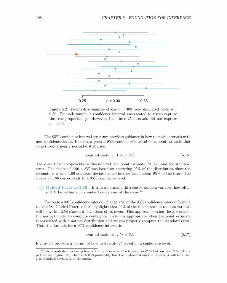
We can be 95% confident that a 95% confidence interval contains the true populationparameter. However, confidence intervals are imperfect. About 1-in-20 (5%) properly con-structed 95% confidence intervals will fail to capture the parameter of interest. Figure 5.2shows 25 confidence intervals for a proportion that were constructed from simulations wherethe true proportion was p = 0.3. However, 1 of these 25 confidence intervals happened notto include the true value.⊙

Guided Practice 5.13 In Figure 5.2, one interval does not contain the true pro-portion, p = 0.3. Does this imply that there was a problem with the simulationsrun?4

5.2.3 Changing the confidence level

Suppose we want to consider confidence intervals where the confidence level is somewhathigher than 95%: perhaps we would like a confidence level of 99%.

Example 5.14 Would a 99% confidence interval be wider or narrower than a 95%confidence interval?

Using a previous analogy: if we want to be more confident that we will catch a fish,we should use a wider net, not a smaller one. To be 99% confidence of capturing thetrue value, we must use a wider interval. On the other hand, if we want an intervalwith lower confidence, such as 90%, we would use a narrower interval.

4No. Just as some observations occur more than 1.96 standard deviations from the mean, some pointestimates will be more than 1.96 standard errors from the parameter. A confidence interval only providesa plausible range of values for a parameter. While we might say other values are implausible based on thedata, this does not mean they are impossible.


0.25 p = 0.30 0.35

●

●

●

●

●

●

●

●

●

●

●

●

●

●

●

●●●

●

●

●

●

●

●

●

●

Figure 5.2: Twenty-five samples of size n = 300 were simulated when p =0.30. For each sample, a confidence interval was created to try to capturethe true proportion p. However, 1 of these 25 intervals did not capturep = 0.30.

The 95% confidence interval structure provides guidance in how to make intervals withnew confidence levels. Below is a general 95% confidence interval for a point estimate thatcomes from a nearly normal distribution:


There are three components to this interval: the point estimate, “1.96”, and the standarderror. The choice of 1.96 × SE was based on capturing 95% of the distribution since theestimate is within 1.96 standard deviations of the true value about 95% of the time. Thechoice of 1.96 corresponds to a 95% confidence level.⊙

Guided Practice 5.16 If X is a normally distributed random variable, how oftenwill X be within 2.58 standard deviations of the mean?5

To create a 99% confidence interval, change 1.96 in the 95% confidence interval formulato be 2.58. Guided Practice 5.16 highlights that 99% of the time a normal random variablewill be within 2.58 standard deviations of its mean. This approach – using the Z scores inthe normal model to compute confidence levels – is appropriate when the point estimateis associated with a normal distribution and we can properly compute the standard error.Thus, the formula for a 99% confidence interval is


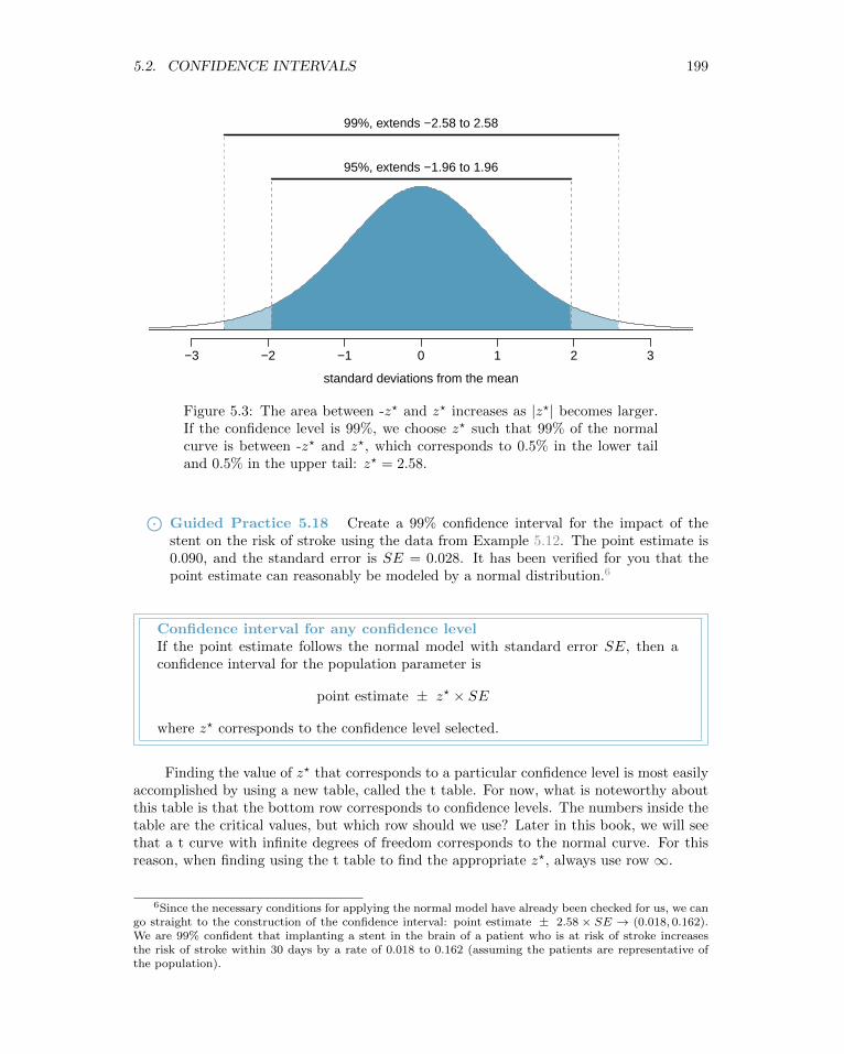
Figure 5.3 provides a picture of how to identify z? based on a confidence level.

5This is equivalent to asking how often the Z score will be larger than -2.58 but less than 2.58. (For apicture, see Figure 5.3.) There is ≈ 0.99 probability that the unobserved random variable X will be within2.58 standard deviations of the mean.


standard deviations from the mean

−3 −2 −1 0 1 2 3

95%, extends −1.96 to 1.96

99%, extends −2.58 to 2.58

Figure 5.3: The area between -z? and z? increases as |z?| becomes larger.If the confidence level is 99%, we choose z? such that 99% of the normalcurve is between -z? and z?, which corresponds to 0.5% in the lower tailand 0.5% in the upper tail: z? = 2.58.

⊙Guided Practice 5.18 Create a 99% confidence interval for the impact of thestent on the risk of stroke using the data from Example 5.12. The point estimate is0.090, and the standard error is SE = 0.028. It has been verified for you that thepoint estimate can reasonably be modeled by a normal distribution.6

Confidence interval for any confidence levelIf the point estimate follows the normal model with standard error SE, then aconfidence interval for the population parameter is

point estimate ± z? × SE

where z? corresponds to the confidence level selected.

Finding the value of z? that corresponds to a particular confidence level is most easilyaccomplished by using a new table, called the t table. For now, what is noteworthy aboutthis table is that the bottom row corresponds to confidence levels. The numbers inside thetable are the critical values, but which row should we use? Later in this book, we will seethat a t curve with infinite degrees of freedom corresponds to the normal curve. For thisreason, when finding using the t table to find the appropriate z?, always use row ∞.

6Since the necessary conditions for applying the normal model have already been checked for us, we cango straight to the construction of the confidence interval: point estimate ± 2.58 × SE → (0.018, 0.162).We are 99% confident that implanting a stent in the brain of a patient who is at risk of stroke increasesthe risk of stroke within 30 days by a rate of 0.018 to 0.162 (assuming the patients are representative ofthe population).


one tail 0.100 0.050 0.025 0.010 0.005df 1 3.078 6.314 12.71 31.82 63.66

2 1.886 2.920 4.303 6.965 9.9253 1.638 2.353 3.182 4.541 5.841...

......

......

1000 1.282 1.646 1.962 2.330 2.581∞ 1.282 1.645 1.960 2.326 2.576

Confidence level C 80% 90% 95% 98% 99%

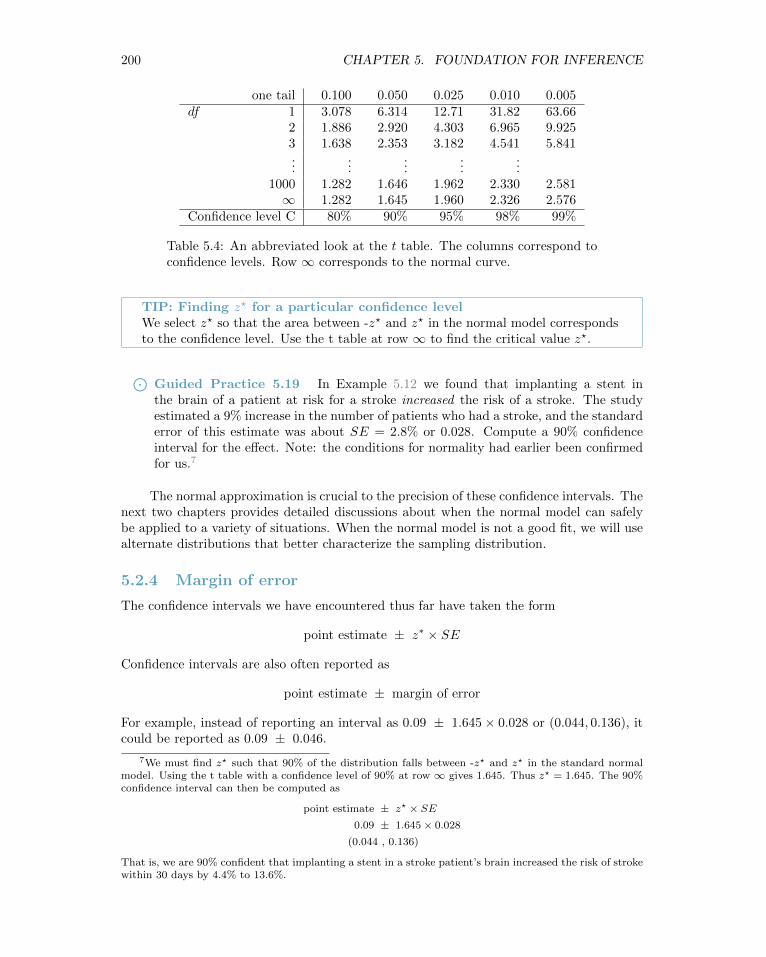
Table 5.4: An abbreviated look at the t table. The columns correspond toconfidence levels. Row ∞ corresponds to the normal curve.

TIP: Finding z? for a particular confidence levelWe select z? so that the area between -z? and z? in the normal model correspondsto the confidence level. Use the t table at row ∞ to find the critical value z?.

⊙Guided Practice 5.19 In Example 5.12 we found that implanting a stent inthe brain of a patient at risk for a stroke increased the risk of a stroke. The studyestimated a 9% increase in the number of patients who had a stroke, and the standarderror of this estimate was about SE = 2.8% or 0.028. Compute a 90% confidenceinterval for the effect. Note: the conditions for normality had earlier been confirmedfor us.7

The normal approximation is crucial to the precision of these confidence intervals. Thenext two chapters provides detailed discussions about when the normal model can safelybe applied to a variety of situations. When the normal model is not a good fit, we will usealternate distributions that better characterize the sampling distribution.

5.2.4 Margin of error

The confidence intervals we have encountered thus far have taken the form

point estimate ± z∗ × SE

Confidence intervals are also often reported as

point estimate ± margin of error

For example, instead of reporting an interval as 0.09 ± 1.645× 0.028 or (0.044, 0.136), itcould be reported as 0.09 ± 0.046.

7We must find z? such that 90% of the distribution falls between -z? and z? in the standard normalmodel. Using the t table with a confidence level of 90% at row ∞ gives 1.645. Thus z? = 1.645. The 90%confidence interval can then be computed as

point estimate ± z? × SE0.09 ± 1.645× 0.028

(0.044 , 0.136)

That is, we are 90% confident that implanting a stent in a stroke patient’s brain increased the risk of strokewithin 30 days by 4.4% to 13.6%.


The margin of error is the distance between the point estimate and the lower orupper bound of a confidence interval.

Margin of errorA confidence interval can be written as point estimate ± margin of error.For a confidence interval for a proportion, the margin of error is z? × SE.

⊙Guided Practice 5.20 To have a smaller margin or error, should one use a largersample or a smaller sample?8

⊙Guided Practice 5.21 What is the margin of error for the confidence interval:(0.035, 0.145)?9

5.2.5 Interpreting confidence intervals

A careful eye might have observed the somewhat awkward language used to describe con-fidence intervals. Correct interpretation:

We are [XX]% confident that the population parameter is between...

Incorrect language might try to describe the confidence interval as capturing the populationparameter with a certain probability.10 This is one of the most common errors: while itmight be useful to think of it as a probability, the confidence level only quantifies howplausible it is that the parameter is in the interval.

As we saw in Figure 5.2, the 95% confidence interval method has a 95% probability ofproducing an interval that will contain the population parameter. However, each individualinterval either does or does not contain the population parameter.

Another especially important consideration of confidence intervals is that they onlytry to capture the population parameter. Our intervals say nothing about the confidenceof capturing individual observations, a proportion of the observations, or about capturingpoint estimates. Confidence intervals only attempt to capture population parameters.

8Intuitively, a larger sample should tend to yield less error. We can also note that n, the sample size isin the denominator of the SE formula, so a n goes up, the SE and thus the margin of error go down.

9Because we both add and subtract the margin of error to get the confidence interval, the margin oferror is half of the width of the interval. (0.145− 0.035)/2 = 0.055.

10To see that this interpretation is incorrect, imagine taking two random samples and constructing two95% confidence intervals for an unknown proportion. If these intervals are disjoint, can we say that thereis a 95%+95%=190% chance that the first or the second interval captures the true value?


5.2.6 Using confidence intervals: a stepwise approach

Follow these six steps when carrying out any confidence interval problem.

Steps for using confidence intervals (AP exam tip) The AP exam is scoredin a standardized way, so to ensure full points for a problem, make sure to completeeach of the following steps.

1. State the name of the CI being used.

2. Verify conditions to ensure the standard error estimate is reasonable andthe point estimate is unbiased and follows the expected distribution, often anormal distribution.

3. Plug in the numbers and write the interval in the form

point estimate ± critical value× SE of estimate

So far, the critical value has taken the form z?.

4. Evaluate the CI and write in the form ( , ).

5. Interpret the interval: “We are [XX]% confident that the true [describe theparameter in context] falls between [identify the upper and lower endpointsof the calculated interval].

6. State your conclusion to the original question. (Sometimes, as in the case ofthe examples in this section, no conclusion is necessary.)

5.3 Introducing Hypothesis testing

Example 5.22 Suppose your professor splits the students in class into two groups:students on the left and students on the right. If p̂

Land p̂

Rrepresent the proportion

of students who own an Apple product on the left and right, respectively, would yoube surprised if p̂

Ldid not exactly equal p̂

R?

While the proportions would probably be close to each other, they are probably notexactly the same. We would probably observe a small difference due to chance.

Studying randomness of this form is a key focus of statistics. How large would theobserved difference in these two proportions need to be for us to believe that there is a realdifference in Apple ownership? In this section, we’ll explore this type of randomness in thecontext of an unknown proportion, and we’ll learn new tools and ideas that will be appliedthroughout the rest of the book.

5.3.1 Case study: medical consultant

People providing an organ for donation sometimes seek the help of a special medical con-sultant. These consultants assist the patient in all aspects of the surgery, with the goalof reducing the possibility of complications during the medical procedure and recovery.Patients might choose a consultant based in part on the historical complication rate of theconsultant’s clients.

5.3. INTRODUCING HYPOTHESIS TESTING 203

One consultant tried to attract patients by noting the average complication rate forliver donor surgeries in the US is about 10%, but her clients have had only 3 complicationsin the 62 liver donor surgeries she has facilitated. She claims this is strong evidence thather work meaningfully contributes to reducing complications (and therefore she shouldbe hired!).

Example 5.23 We will let p represent the true complication rate for liver donorsworking with this consultant. Estimate p using the data, and label this value p̂.

The sample proportion for the complication rate is 3 complications divided by the62 surgeries the consultant has worked on: p̂ = 3/62 = 0.048.

Example 5.24 Is it possible to prove that the consultant’s work reduces complica-tions?

No. The claim implies that there is a causal connection, but the data are observa-tional. For example, maybe patients who can afford a medical consultant can affordbetter medical care, which can also lead to a lower complication rate.

Example 5.25 While it is not possible to assess the causal claim, it is still possibleto ask whether the low complication rate of p̂ = 0.048 provides evidence that theconsultant’s true complication rate is different than the average complication rate inthe US. Why might we be tempted to immediately conclude that the consultant’strue complication rate is different than the average complication rate? Can we drawthis conclusion?

Her sample complication rate is p̂ = 0.048, 0.052 lower than the average complicationrate in the US of 10%. However, we cannot yet be sure if the observed differencerepresents a real difference or is just the result of random variation. We wouldn’texpect the sample proportion to be exactly 0.10, even if the truth was that her realcomplication rate was 0.10.

5.3.2 Setting up the null and alternate hypothesis

We can set up two competing hypotheses about the consultant’s true complication rate.The first is call the null hypothesis and represents either a skeptical perspective or aperspective of no difference. The second is called the alternative hypothesis (or alternatehypothesis) and represents a new perspective such as the possibility that there has been achange or that there is a treatment effect in an experiment.

Null and alternative hypotheses

The null hypothesis is abbreviated H0. It states that nothing has changed andthat any deviation from what was expected is due to chance error.

The alternative hypothesis is abbreviated HA. It asserts that there has beena change and that the observed deviation is too large to be explained bychance alone.


Example 5.26 Identify the null and alternative claim regarding the consultant’scomplication rate.

H0: The true complication rate for the consultant’s clients is the same as the averagecomplication rate in the US of 10%.

HA: The true complication rate for the consultant’s clients is different than 10%.

Often it is convenient to write the null and alternative hypothesis in mathematical ornumerical terms. To do so, we must first identify the quantity of interest. This quantity ofinterest is known as the parameter for a hypothesis test.

Parameters and point estimates

A parameter for a hypothesis test is the “true” value of the population of inter-est. When the parameter is a proportion, we call it p.

A point estimate is calculated from a sample. When the point estimate is aproportion, we call it p̂.

The observed or sample proportion 0f 0.048 is a point estimate for the true proportion.The parameter in this problem is the true proportion of complications for this consultant’sclients. The parameter is unknown, but the null hypothesis is that it equals the overallproportion of complications: p = 0.10. This hypothesized value is called the null value.

Null value of a hypothesis testThe null value is the value hypothesized for the parameter in H0, and it is some-times represented with a subscript 0, e.g. p0 (just like H0).

In the medical consultant case study, the parameter is p and the null value is p0 = 0.10.We can write the null and alternative hypothesis as numerical statements as follows.

• H0: p = 0.10 (The complication rate for the consultant’s clients is equal to the USaverage of 10%.)

• HA: p 6= 0.10 (The complication rate for the consultant’s clients is not equal to theUS average of 10%.)

Hypothesis testingThese hypotheses are part of what is called a hypothesis test. A hypothesistest is a statistical technique used to evaluate competing claims using data. Oftentimes, the null hypothesis takes a stance of no difference or no effect. If the nullhypothesis and the data notably disagree, then we will reject the null hypothesisin favor of the alternative hypothesis.

Don’t worry if you aren’t a master of hypothesis testing at the end of this sec-tion. We’ll discuss these ideas and details many times in this chapter and the twochapters that follow.

The null claim is always framed as an equality: it tells us what quantity we should usefor the parameter when calculating the p-value. There are three choices for the alternative


hypothesis, depending upon whether the researcher is trying to prove that the value of theparameter is greater than, less than, or not equal to the null value.

TIP: Always write the null hypothesis as an equalityWe will find it most useful if we always list the null hypothesis as an equality(e.g. p = 7) while the alternative always uses an inequality (e.g. p 6= 0.7, p > 0.7,or p < 0.7).

⊙Guided Practice 5.27 According to US census data, in 2012 the percent of maleresidents in the state of Alaska was 52.1%.11 A researcher plans to take a randomsample of residents from Alaska to test whether or not this is still the case. Writeout the hypotheses that the researcher should test in both plain and statistical lan-guage. 12

When the alternative claim uses a 6=, we call the test a two-sided test, because eitherextreme provides evidence against H0. When the alternative claim uses a < or a >, we callit a one-sided test.

TIP: One-sided and two-sided testsIf the researchers are only interested in showing an increase or a decrease, but notboth, use a one-sided test. If the researchers would be interested in any differencefrom the null value – an increase or decrease – then the test should be two-sided.

Example 5.28 For the example of the consultant’s complication rate, we knew thather sample complication rate was 0.048, which was lower than average US complica-tion rate of 0.10. Why did we conduct a two-sided hypothesis test for this setting?

The setting was framed in the context of the consultant being helpful, but what if theconsultant actually performed worse than the average? Would we care? More thanever! Since we care about a finding in either direction, we should run a two-sided test.

Caution: One-sided hypotheses are allowed only before seeing dataAfter observing data, it is tempting to turn a two-sided test into a one-sided test.Avoid this temptation. Hypotheses must be set up before observing the data.If they are not, the test must be two-sided.

5.3.3 Evaluating the hypotheses with a p-value

Example 5.29 There were 62 patients in the consultant’s sample. If the null claimis true, how many would we expect to have had a complication?

If the null claim is true, we would expect about 10% of the patients, or about 6.2 tohave a complication.

11http://www.census.gov/newsroom/releases/archives/population/cb13-112.html12H0: p = 0.521; The proportion of male residents in Alaska is unchanged from 2012. HA: p 6= 0.521;

The proportion of male residents in Alaska has changed from 2012. Note that it could have increased ordecreased.

http://www.census.gov/newsroom/releases/archives/population/cb13-112.html


The complication rate in the consultant’s sample of size 62 was 0.048 (0.048×62 ≈ 3).What is the probability that a sample would produce a number of complications rates thisfar from the expected value of 6.2, if her true complication rate were 0.10, that is, if H0

were true. The probability, which is estimated in the section that follows, turns out the be0.2444. We call his quantity the p-value.

Interpreting the p-valueThe p-value is the probability of observing data at least as favorable to the alter-native hypothesis as our current data set, if the null hypothesis were true.When examining a a proportion we can also interpret the p-value as follows, de-pending upon the nature of the alternative hypothesis.

When the p-value is small, i.e. less than a previously set threshold, we say the resultsare statistically significant. This means the data provide such strong evidence againstH0 that we reject the null hypothesis in favor of the alternative hypothesis. The thresh-old, called the significance level and often represented by α (the Greek letter alpha), is

αsignificancelevel of ahypothesis test

typically set to α = 0.05, but can vary depending on the field or the application. Using asignificance level of α = 0.05 in the discrimination study, we can say that the data providedstatistically significant evidence against the null hypothesis.

Statistical significanceWe say that the data provide statistically significant evidence against the nullhypothesis if the p-value is less than some reference value, usually α = 0.05.

Recall that the null claim is the claim of no difference. If we reject H0, we are assertingthat there is a real difference. If we do not reject H0, we are saying that the null claim isreasonable. That is, we have not disproved it.

⊙Guided Practice 5.30 Because the p-value is 0.2444, which is larger than thesignificance level 0.05, we do not reject the null hypothesis. Explain what this meansin the context of the problem using plain language.13

Example 5.31 In the previous exercise, we did not reject H0. This means that wedid not disprove the null claim. Is this equivalent to proving the null claim is true?

No. We did not prove that the consultant’s complication rate is exactly equal to 10%.Recall that the test of hypothesis starts by assuming the null claim is true. That is,the test proceeds as an argument by contradiction. If the null claim is true, there is a0.2444 chance of seeing sample data as divergent from 10% as we saw in our sample.Because 0.2444 is large, it is within the realm of chance error and we cannot say thenull hypothesis is unreasonable.14

13The data do not provide evidence that the consultant’s complication rate is significantly lower orhigher that the average US rate of 10%.

14The p-value is actually a conditional probability. It is P(getting data at least as divergent from thenull value as we observed | H0 is true). It is NOT P( H0 is true | we got data this divergent from the nullvalue.


TIP: Double negatives can sometimes be used in statisticsIn many statistical explanations, we use double negatives. For instance, we mightsay that the null hypothesis is not implausible or we failed to reject the null hypoth-esis. Double negatives are used to communicate that while we are not rejecting aposition, we are also not saying that we know it to be true.

Example 5.32 Does the conclusion in Guided Practice 5.30 imply for certain thereis no real association between the surgical consultant’s work and the risk of compli-cations? Explain.

No. It might be that the consultant’s work is associated with a lower or higher riskof complications. However, the data did not provide enough information to reject thenull hypothesis.

Example 5.33 An experiment was conducted where study participants were ran-domly divided into two groups. Both were given the opportunity to purchase a DVD,but the one half was reminded that the money, if not spent on the DVD, could beused for other purchases in the future while the other half was not. The half thatwere reminded that the money could be used on other purchases were 20% less likelyto continue with a DVD purchase. We determined that such a large difference wouldonly occur about 1-in-150 times if the reminder actually had no influence on studentdecision-making. What is the p-value in this study? Was the result statisticallysignificant?

The p-value was 0.006 (about 1/150). Since the p-value is less than 0.05, the dataprovide statistically significant evidence that US college students were actually influ-enced by the reminder.

What’s so special about 0.05?We often use a threshold of 0.05 to determine whether a result is statisticallysignificant. But why 0.05? Maybe we should use a bigger number, or maybe asmaller number. If you’re a little puzzled, that probably means you’re readingwith a critical eye – good job! We’ve made a video to help clarify why 0.05 :

www.openintro.org/why05

Sometimes it’s also a good idea to deviate from the standard. We’ll discuss whento choose a threshold different than 0.05 in Section 5.3.6.

Statistical inference is the practice of making decisions and conclusions from data inthe context of uncertainty. Errors do occur, just like rare events, and the data set at handmight lead us to the wrong conclusion. While a given data set may not always lead us toa correct conclusion, statistical inference gives us tools to control and evaluate how oftenthese errors occur.

http://www.openintro.org/why05


5.3.4 Calculating the p-value by simulation (special topic)

When conditions for the applying the normal model are met, we use the normal model tofind the p-value of a test of hypothesis. In the complication rate example, the distributionis not normal. It is, however, binomial, because we are interested in how many out of 62patients will have complications.

We could calculate the p-value of this test using binomial probabilities. A more generalapproach, though, for calculating p-values when the normal model does not apply is to usewhat is known as simulation. While performing this procedure is outside of the scopeof the course, we provide an example here in order to better understand the concept of ap-value.

We simulate 62 new patients to see what result might happen if the complication ratereally is 0.10. To do this, we could use a deck of cards. Take one red card, nine blackcards, and mix them up. If the cards are well-shuffled, drawing the top card is one way ofsimulating the chance a patient has a complication if the true rate is 0.10: if the card isred, we say the patient had a complication, and if it is black then we say they did not havea complication. If we repeat this process 62 times and compute the proportion of simulatedpatients with complications, p̂sim, then this simulated proportion is exactly a draw fromthe null distribution.

There were 5 simulated cases with a complication and 57 simulated cases without acomplication: p̂sim = 5/62 = 0.081.

One simulation isn’t enough to get a sense of the null distribution, so we repeated thesimulation 10,000 times using a computer. Figure 5.5 shows the null distribution from these10,000 simulations. The simulated proportions that are less than or equal to p̂ = 0.048 areshaded. There were 1222 simulated sample proportions with p̂sim ≤ 0.048, which representsa fraction 0.1222 of our simulations:

left tail =Number of observed simulations with p̂sim ≤ 0.048

10000=

1222

10000= 0.1222

However, this is not our p-value! Remember that we are conducting a two-sided test, sowe should double the one-tail area to get the p-value:15

p-value = 2× left tail = 2× 0.1222 = 0.2444

5.3.5 Decision errors

The hypothesis testing framework is a very general tool, and we often use it without asecond thought. If a person makes a somewhat unbelievable claim, we are initially skeptical.However, if there is sufficient evidence that supports the claim, we set aside our skepticism.The hallmarks of hypothesis testing are also found in the US court system.

Example 5.34 A US court considers two possible claims about a defendant: she iseither innocent or guilty. If we set these claims up in a hypothesis framework, whichwould be the null hypothesis and which the alternative?

The jury considers whether the evidence is so convincing (strong) that there is noreasonable doubt regarding the person’s guilt. That is, the skeptical perspective (nullhypothesis) is that the person is innocent until evidence is presented that convincesthe jury that the person is guilty (alternative hypothesis).

15This doubling approach is preferred even when the distribution isn’t symmetric, as in this case.


p̂sim

0.00 0.05 0.10 0.15 0.20 0.25

0

500

1000

1500

Num

ber

of s

imul

atio

ns

Figure 5.5: The null distribution for p̂, created from 10,000 simulated stud-ies. The left tail contains 12.22% of the simulations. We double this valueto get the p-value.

Jurors examine the evidence to see whether it convincingly shows a defendant is guilty.Notice that if a jury finds a defendant not guilty, this does not necessarily mean the jury isconfident in the person’s innocence. They are simply not convinced of the alternative thatthe person is guilty.

This is also the case with hypothesis testing: even if we fail to reject the null hypothesis,we typically do not accept the null hypothesis as truth. Failing to find strong evidence forthe alternative hypothesis is not equivalent to providing evidence that the null hypothesisis true.

Hypothesis tests are not flawless. Just think of the court system: innocent people aresometimes wrongly convicted and the guilty sometimes walk free. Similarly, data can pointto the wrong conclusion. However, what distinguishes statistical hypothesis tests from acourt system is that our framework allows us to quantify and control how often the datalead us to the incorrect conclusion.

There are two competing hypotheses: the null and the alternative. In a hypothesistest, we make a statement about which one might be true, but we might choose incorrectly.There are four possible scenarios in a hypothesis test, which are summarized in Table 5.6.

Test conclusion

do not reject H0 reject H0 in favor of HA

H0 true okay Type 1 ErrorTruth

HA true Type 2 Error okay

Table 5.6: Four different scenarios for hypothesis tests.

A Type 1 Error is rejecting the null hypothesis when H0 is actually true. When wreject the null hypothesis, it is possible that we make a Type 1 Error. A Type 2 Error isfailing to reject the null hypothesis when the alternative is actually true.

Example 5.35 In a US court, the defendant is either innocent (H0) or guilty (HA).What does a Type 1 Error represent in this context? What does a Type 2 Errorrepresent? Table 5.6 may be useful.

If the court makes a Type 1 Error, this means the defendant is innocent (H0 true) butwrongly convicted. A Type 2 Error means the court failed to reject H0 (i.e. failed toconvict the person) when she was in fact guilty (HA true).


⊙Guided Practice 5.36 A group of women bring a class action law suit that claimsdiscrimination in promotion rates. What would a Type 1 Error represent in thiscontext?16

Example 5.37 How could we reduce the Type 1 Error rate in US courts? Whatinfluence would this have on the Type 2 Error rate?

To lower the Type 1 Error rate, we might raise our standard for conviction from“beyond a reasonable doubt” to “beyond a conceivable doubt” so fewer people wouldbe wrongly convicted. However, this would also make it more difficult to convict thepeople who are actually guilty, so we would make more Type 2 Errors.

⊙Guided Practice 5.38 How could we reduce the Type 2 Error rate in US courts?What influence would this have on the Type 1 Error rate?17

The example and Exercise above provide an important lesson: if we reduce how oftenwe make one type of error, we generally make more of the other type.

5.3.6 Choosing a significance level

Choosing a significance level for a test is important in many contexts, and the traditionallevel is 0.05. However, it is sometimes helpful to adjust the significance level based on theapplication. We may select a level that is smaller or larger than 0.05 depending on theconsequences of any conclusions reached from the test.

If making a Type 1 Error is dangerous or especially costly, we should choose a smallsignificance level (e.g. 0.01 or 0.001). Under this scenario, we want to be very cautiousabout rejecting the null hypothesis, so we demand very strong evidence favoring the alter-native HA before we would reject H0.

If a Type 2 Error is relatively more dangerous or much more costly than a Type 1Error, then we should choose a higher significance level (e.g. 0.10). Here we want to becautious about failing to reject H0 when the null is actually false.

TIP: Significance levels should reflect consequences of errorsThe significance level selected for a test should reflect the real-world consequencesassociated with making a Type 1 or Type 2 Error.

16We must first identify which is the null hypothesis and which is the alternative. The alternativehypothesis is the one that bears the burden of proof, so the null hypothesis is that there was no discrim-ination and the alternative hypothesis is that there was descrimination. Making a Type 1 Error in thiscontext would mean that in fact there was no discrimination, even though we concluded that women werediscriminated against. Notice that this does not necessarily mean something was wrong with the data orthat we made a computational mistake. Sometimes data simply point us to the wrong conclusion, whichis why scientific studies are often repeated to check initial findings.

17To lower the Type 2 Error rate, we want to convict more guilty people. We could lower the standardsfor conviction from “beyond a reasonable doubt” to “beyond a little doubt”. Lowering the bar for guiltwill also result in more wrongful convictions, raising the Type 1 Error rate.

5.4. DOES IT MAKE SENSE? 211

5.3.7 Formal hypothesis testing: a stepwise approach

Carrying out a formal test of hypothesis (AP exam tip)Follow these seven steps when carrying out a hypothesis test.

1. State the name of the test being used.

2. Verify conditions to ensure the standard error estimate is reasonable and thepoint estimate follows appropriate distribution and is unbiased.

3. First write the hypotheses in plain language, then set them up in mathemat-ical notation.

4. Identify the significance level α.

5. Calculate the test statistic, often Z, using an appropriate point estimate ofthe parameter of interest and its standard error.

test statistic =point estimate− null value

SE of estimate

6. Find the p-value, compare it to α, and state whether to reject or not rejectthe null hypothesis.

7. Write your conclusion.

5.4 Does it make sense?

5.4.1 When to retreat

Statistical tools rely on conditions. When the conditions are not met, these tools areunreliable and drawing conclusions from them is treacherous. The conditions for thesetools typically come in two forms.

• The individual observations must be independent. A random sample from lessthan 10% of the population ensures the observations are independent. In experiments,we generally require that subjects are randomized into groups. If independence fails,then advanced techniques must be used, and in some such cases, inference may notbe possible.

• Other conditions focus on sample size and skew. For example, if the samplesize is too small, the skew too strong, or extreme outliers are present, then the normalmodel for the sample mean will fail.

Verification of conditions for statistical tools is always necessary. Whenever conditions arenot satisfied for a statistical technique, there are three options. The first is to learn newmethods that are appropriate for the data. The second route is to consult a statistician.18

The third route is to ignore the failure of conditions. This last option effectively invalidatesany analysis and may discredit novel and interesting findings.

Finally, we caution that there may be no inference tools helpful when considering datathat include unknown biases, such as convenience samples. For this reason, there are books,

18If you work at a university, then there may be campus consulting services to assist you. Alternatively,there are many private consulting firms that are also available for hire.


courses, and researchers devoted to the techniques of sampling and experimental design.See Sections 1.3-1.5 for basic principles of data collection.

5.4.2 Statistical significance versus practical significance

When the sample size becomes larger, point estimates become more precise and any realdifferences in the mean and null value become easier to detect and recognize. Even avery small difference would likely be detected if we took a large enough sample. Some-times researchers will take such large samples that even the slightest difference is detected.While we still say that difference is statistically significant, it might not be practicallysignificant.

Statistically significant differences are sometimes so minor that they are not practicallyrelevant. This is especially important to research: if we conduct a study, we want to focuson finding a meaningful result. We don’t want to spend lots of money finding results thathold no practical value.

The role of a statistician in conducting a study often includes planning the size ofthe study. The statistician might first consult experts or scientific literature to learn whatwould be the smallest meaningful difference from the null value. She also would obtain somereasonable estimate for the standard deviation. With these important pieces of information,she would choose a sufficiently large sample size so that the power for the meaningfuldifference is perhaps 80% or 90%. While larger sample sizes may still be used, she mightadvise against using them in some cases, especially in sensitive areas of research.

5.4.3 Statistical power of a hypothesis test

When the alternative hypothesis is true, the probability of not making a Type 2 Error iscalled power. It is common for researchers to perform a power analysis to ensure their studycollects enough data to detect the effects they anticipate finding. As you might imagine, ifthe effect they care about is small or subtle, then if the effect is real, the researchers willneed to collect a large sample size in order to have a good chance of detecting the effect.However, if they are interested in large effect, they need not collect as much data.

The Type 2 Error rate β and the magnitude of the error for a point estimate arecontrolled by the sample size. Real differences from the null value, even large ones, maybe difficult to detect with small samples. If we take a very large sample, we might finda statistically significant difference but the magnitude might be so small that it is of nopractical value.

Chapter 7

Inference for numerical data

Chapter 5 introduced a framework for statistical inference based on confidence intervalsand hypotheses. Chapter 6 summarized inference procedures for categorical data (countsand proportions). In this chapter, we focus on inference procedures for numerical data andwe encounter several new point estimates and scenarios. In each case, the inference ideasremain the same:

1. Determine which point estimate or test statistic is useful.

2. Identify an appropriate distribution for the point estimate or test statistic.

3. Apply the ideas from Chapter 5 using the distribution from step 2.

Each section in Chapter 7 explores a new situation: a single mean (7.1), the mean ofdifferences (7.2), the difference between means (7.3); and the comparison of means acrossmultiple groups (7.4).

7.1 Inference for a single mean with the t distribution

When certain conditions are satisfied, the sampling distribution associated with a samplemean or difference of two sample means is nearly normal. However, this becomes morecomplex when the sample size is small, where small here typically means a sample sizesmaller than 30 observations. For this reason, we’ll use a new distribution called the tdistribution that will often work for both small and large samples of numerical data.

7.1.1 Using the Z distribution for inference when µ is unknownand σ is known

We have seen in Section 4.2 that the distribution of a sample mean is normal if the popula-tion is normal or if the sample size is at least 30. In these problems, we used the populationmean and population standard deviation to find a Z score. However, in the case of infer-ence, the parameters will be unknown. In rare circumstances we may know the standarddeviation of a population, even though we do not know its mean. For example, in someindustrial process, the mean may be known to shift over time, while the standard deviationof the process remains the same. In these cases, we can use the normal model as the basisfor our inference procedures. We use x̄ as our point estimate for µ and the SD formula

268

7.1. INFERENCE FOR A SINGLE MEAN WITH THE T DISTRIBUTION 269

calculated in Section 4.2: SD = σ√n

.

CI: x̄ ± Z∗σ√n

Z =x̄− null value

σ√n

What happens if we do not know the population standard deviation σ, as is usually thecase? The best we can do is use the sample standard deviation, denoted by s, to estimatethe population standard deviation.

SE =s√n

However, when we do this we run into a problem: when carrying out our inference pro-cedures we will be trying to estimate two quantities: both the mean and the standarddeviation. Looking at the SD and SE formulas, we can make some important observationsthat will give us a hint as to what will happen when we use s instead of σ.

• For a given population, σ is a fixed number and does not vary.

• s, the standard deviation of a sample, will vary from one sample to the next and willnot be exactly equal to σ.

• The larger the sample size n, the better the estimate s will tend to be for σ.

For this reason, the normal model still works well when the sample size is larger thanabout 30. For smaller sample sizes, we run into a problem: our estimate of s, which is usedto compute the standard error, isn’t as reliable and tends to add more variability to ourestimate of the mean. It is this extra variability that leads us to a new distribution: thet distribution.

7.1.2 Introducing the t distribution

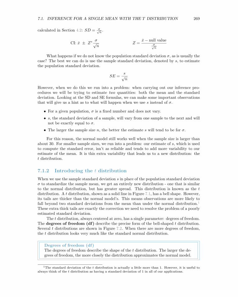
When we use the sample standard deviation s in place of the population standard deviationσ to standardize the sample mean, we get an entirely new distribution - one that is similarto the normal distribution, but has greater spread. This distribution is known as the tdistribution. A t distribution, shown as a solid line in Figure 7.1, has a bell shape. However,its tails are thicker than the normal model’s. This means observations are more likely tofall beyond two standard deviations from the mean than under the normal distribution.1

These extra thick tails are exactly the correction we need to resolve the problem of a poorlyestimated standard deviation.

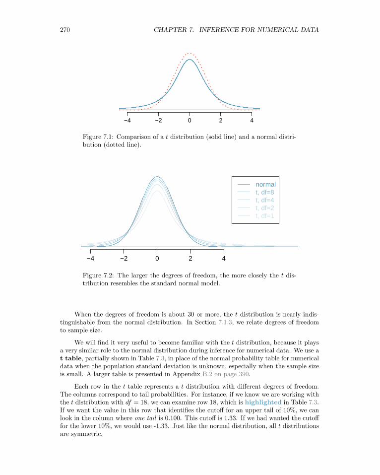
The t distribution, always centered at zero, has a single parameter: degrees of freedom.The degrees of freedom (df) describe the precise form of the bell-shaped t distribution.Several t distributions are shown in Figure 7.2. When there are more degrees of freedom,the t distribution looks very much like the standard normal distribution.

Degrees of freedom (df)The degrees of freedom describe the shape of the t distribution. The larger the de-grees of freedom, the more closely the distribution approximates the normal model.

1The standard deviation of the t distribution is actually a little more than 1. However, it is useful toalways think of the t distribution as having a standard deviation of 1 in all of our applications.

270 CHAPTER 7. INFERENCE FOR NUMERICAL DATA

−4 −2 0 2 4

Figure 7.1: Comparison of a t distribution (solid line) and a normal distri-bution (dotted line).

−4 −2 0 2 4

normalt, df=8t, df=4t, df=2t, df=1

Figure 7.2: The larger the degrees of freedom, the more closely the t dis-tribution resembles the standard normal model.

When the degrees of freedom is about 30 or more, the t distribution is nearly indis-tinguishable from the normal distribution. In Section 7.1.3, we relate degrees of freedomto sample size.

We will find it very useful to become familiar with the t distribution, because it playsa very similar role to the normal distribution during inference for numerical data. We use at table, partially shown in Table 7.3, in place of the normal probability table for numericaldata when the population standard deviation is unknown, especially when the sample sizeis small. A larger table is presented in Appendix B.2 on page 390.

Each row in the t table represents a t distribution with different degrees of freedom.The columns correspond to tail probabilities. For instance, if we know we are working withthe t distribution with df = 18, we can examine row 18, which is highlighted in Table 7.3.If we want the value in this row that identifies the cutoff for an upper tail of 10%, we canlook in the column where one tail is 0.100. This cutoff is 1.33. If we had wanted the cutofffor the lower 10%, we would use -1.33. Just like the normal distribution, all t distributionsare symmetric.


one tail 0.100 0.050 0.025 0.010 0.005df 1 3.078 6.314 12.71 31.82 63.66

2 1.886 2.920 4.303 6.965 9.9253 1.638 2.353 3.182 4.541 5.841...

......

......

17 1.333 1.740 2.110 2.567 2.89818 1.330 1.734 2.101 2.552 2.87819 1.328 1.729 2.093 2.539 2.86120 1.325 1.725 2.086 2.528 2.845

......

......

...1000 1.282 1.646 1.962 2.330 2.581∞ 1.282 1.645 1.960 2.326 2.576

Confidence level C 80% 90% 95% 98% 99%

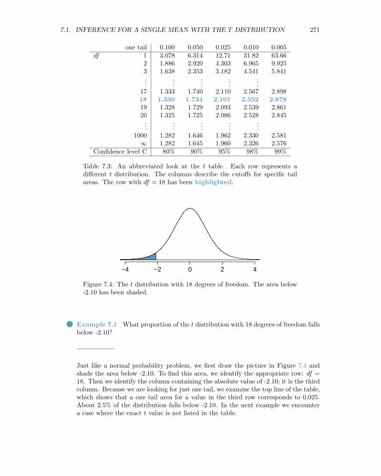
Table 7.3: An abbreviated look at the t table. Each row represents adifferent t distribution. The columns describe the cutoffs for specific tailareas. The row with df = 18 has been highlighted.

−4 −2 0 2 4

Figure 7.4: The t distribution with 18 degrees of freedom. The area below-2.10 has been shaded.

Example 7.1 What proportion of the t distribution with 18 degrees of freedom fallsbelow -2.10?

Just like a normal probability problem, we first draw the picture in Figure 7.4 andshade the area below -2.10. To find this area, we identify the appropriate row: df =18. Then we identify the column containing the absolute value of -2.10; it is the thirdcolumn. Because we are looking for just one tail, we examine the top line of the table,which shows that a one tail area for a value in the third row corresponds to 0.025.About 2.5% of the distribution falls below -2.10. In the next example we encountera case where the exact t value is not listed in the table.


−4 −2 0 2 4

c(0,

dno

rm(0

))

−4 −2 0 2 4

Figure 7.5: Left: The t distribution with 20 degrees of freedom, with thearea above 1.65 shaded. Right: The t distribution with 2 degrees of free-dom, with the area further than 3 units from 0 shaded.

Example 7.2 A t distribution with 20 degrees of freedom is shown in the left panelof Figure 7.5. Estimate the proportion of the distribution falling above 1.65.

We identify the row in the t table using the degrees of freedom: df = 20. Then welook for 1.65; it is not listed. It falls between the first and second columns. Sincethese values bound 1.65, their tail areas will bound the tail area corresponding to1.65. We identify the one tail area of the first and second columns, 0.050 and 0.10,and we conclude that between 5% and 10% of the distribution is more than 1.65standard deviations above the mean. If we like, we can identify the precise area usingstatistical software: 0.0573.

Example 7.3 A t distribution with 2 degrees of freedom is shown in the right panelof Figure 7.5. Estimate the proportion of the distribution falling more than 3 unitsfrom the mean (above or below).

As before, first identify the appropriate row: df = 2. Next, find the columns thatcapture 3; because 2.92 < 3 < 4.30, we use the second and third columns. Finally,we find bounds for the tail areas by looking at the two tail values: 0.05 and 0.10. Weuse the two tail values because we are looking for two (symmetric) tails.

7.1.3 The t distribution and the standard error of a mean

When estimating the mean and standard deviation from a small sample, the t distributionis a more accurate tool than the normal model. This is true for both small and largesamples.

TIP: When to use the t distributionUse the t distribution for inference of the sample mean when observations areindependent and nearly normal. You may relax the nearly normal condition asthe sample size increases. For example, the data distribution may be moderatelyskewed when the sample size is at least 30.


To proceed with the t distribution for inference about a single mean, we must checktwo conditions.

Independence of observations. We verify this condition just as we did before. Wecollect a simple random sample from less than 10% of the population, or if it was anexperiment or random process, we carefully check to the best of our abilities that theobservations were independent.

n ≥ 30 or observations come from a nearly normal distribution. We can easily checkif the sample size is at least 30. If it is not, then this second condition requires morecare. We often (i) take a look at a graph of the data, such as a dot plot or box plot,for obvious departures from the normal model, and (ii) consider whether any previousexperiences alert us that the data may not be nearly normal.

When examining a sample mean and estimated standard deviation from a sample of nindependent and nearly normal observations, we use a t distribution with n− 1 degrees offreedom (df). For example, if the sample size was 19, then we would use the t distributionwith df = 19 − 1 = 18 degrees of freedom and proceed exactly as we did in Chapter 5,except that now we use the t table.

The t distribution and the SE of a meanIn general, when the population mean is uknown, the population standard devi-ation will also be unknown. When this is the case, we estimate the populationstandard deviation with the sample standard deviation and we use SE insteadof SD.

SEx̄ =s√n

When we use the sample standard deviation, we use the t distribution with df =n− 1 degrees of freedom instead of the normal distribution.

7.1.4 The normality condition

When the sample size n is at least 30, the Central Limit Theorem tells us that we do nothave to worry too much about skew in the data. When this is not true, we need verifythat the observations come from a nearly normal distribution. In some cases, this may beknown, such as if the population is the heights of adults.

What do we do, though, if the population is not known to be approximately normalAND the sample size is small? We must look at the distribution of the data and check forexcessive skew.

Caution: Checking the normality conditionWe should exercise caution when verifying the normality condition for small sam-ples. It is important to not only examine the data but also think about wherethe data come from. For example, ask: would I expect this distribution to besymmetric, and am I confident that outliers are rare?

You may relax the normality condition as the sample size goes up. If the sample sizeis 10 or more, slight skew is not problematic. Once the sample size hits about 30, then mod-erate skew is reasonable. Data with strong skew or outliers require a more cautious analysis.


7.1.5 One sample t confidence intervals

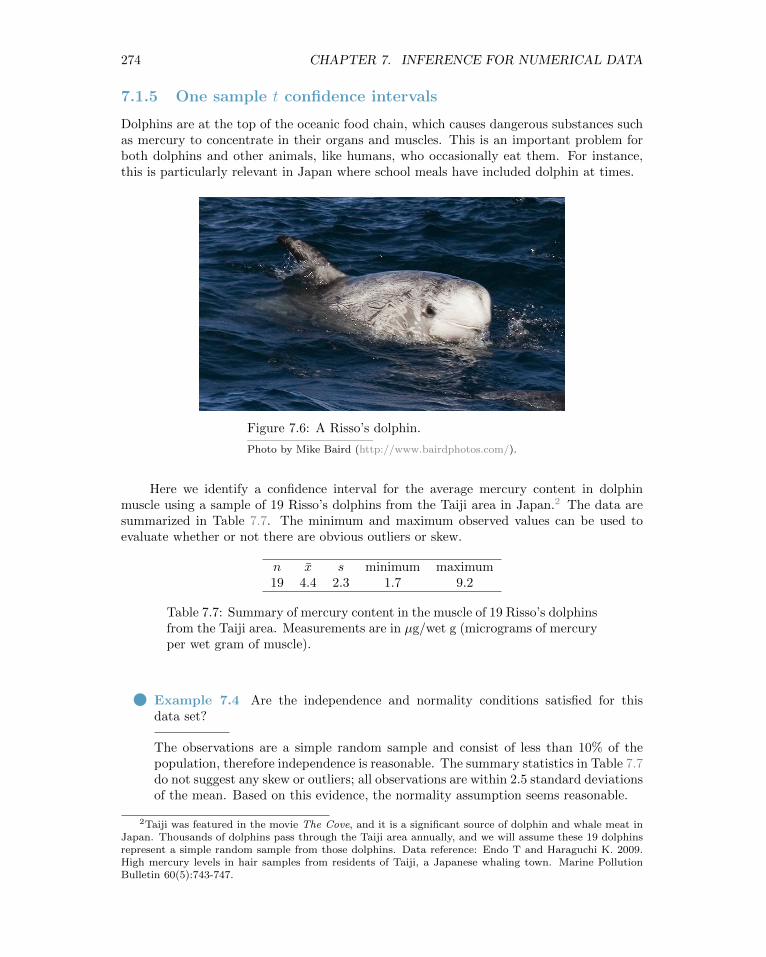
Dolphins are at the top of the oceanic food chain, which causes dangerous substances suchas mercury to concentrate in their organs and muscles. This is an important problem forboth dolphins and other animals, like humans, who occasionally eat them. For instance,this is particularly relevant in Japan where school meals have included dolphin at times.

Figure 7.6: A Risso’s dolphin.—————————–Photo by Mike Baird (http://www.bairdphotos.com/).

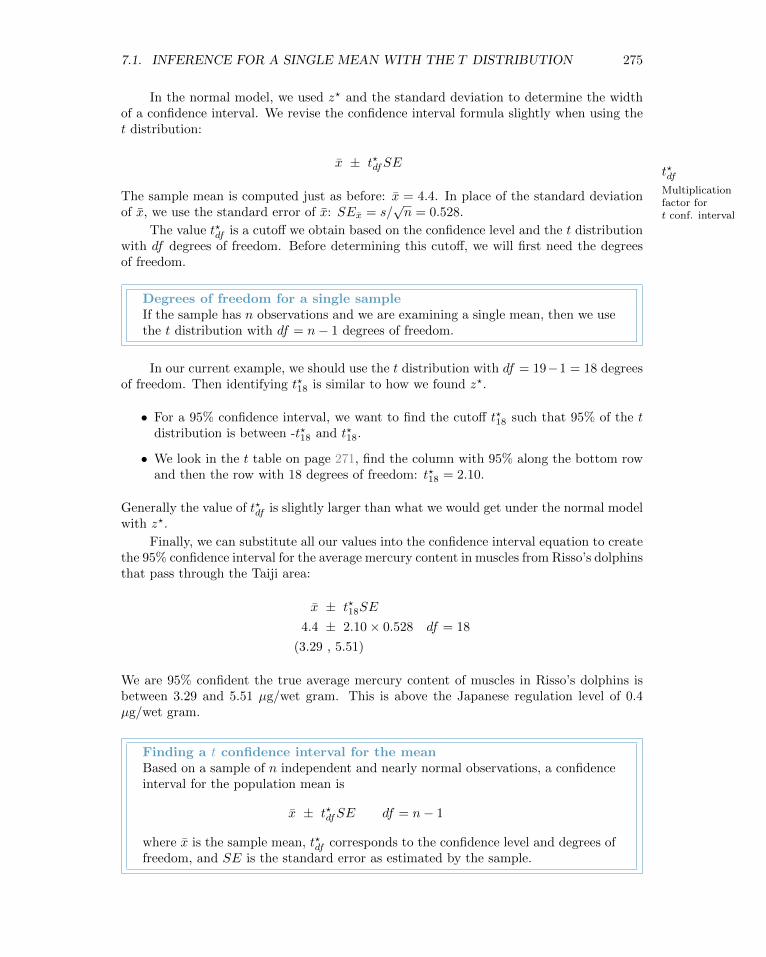
Here we identify a confidence interval for the average mercury content in dolphinmuscle using a sample of 19 Risso’s dolphins from the Taiji area in Japan.2 The data aresummarized in Table 7.7. The minimum and maximum observed values can be used toevaluate whether or not there are obvious outliers or skew.

n x̄ s minimum maximum19 4.4 2.3 1.7 9.2

Table 7.7: Summary of mercury content in the muscle of 19 Risso’s dolphinsfrom the Taiji area. Measurements are in µg/wet g (micrograms of mercuryper wet gram of muscle).

Example 7.4 Are the independence and normality conditions satisfied for thisdata set?

The observations are a simple random sample and consist of less than 10% of thepopulation, therefore independence is reasonable. The summary statistics in Table 7.7do not suggest any skew or outliers; all observations are within 2.5 standard deviationsof the mean. Based on this evidence, the normality assumption seems reasonable.

2Taiji was featured in the movie The Cove, and it is a significant source of dolphin and whale meat inJapan. Thousands of dolphins pass through the Taiji area annually, and we will assume these 19 dolphinsrepresent a simple random sample from those dolphins. Data reference: Endo T and Haraguchi K. 2009.High mercury levels in hair samples from residents of Taiji, a Japanese whaling town. Marine PollutionBulletin 60(5):743-747.

http://www.bairdphotos.com/


In the normal model, we used z? and the standard deviation to determine the widthof a confidence interval. We revise the confidence interval formula slightly when using thet distribution:

x̄ ± t?dfSE

The sample mean is computed just as before: x̄ = 4.4. In place of the standard deviation

t?dfMultiplicationfactor fort conf. intervalof x̄, we use the standard error of x̄: SEx̄ = s/

√n = 0.528.

The value t?df is a cutoff we obtain based on the confidence level and the t distributionwith df degrees of freedom. Before determining this cutoff, we will first need the degreesof freedom.

Degrees of freedom for a single sampleIf the sample has n observations and we are examining a single mean, then we usethe t distribution with df = n− 1 degrees of freedom.

In our current example, we should use the t distribution with df = 19−1 = 18 degreesof freedom. Then identifying t?18 is similar to how we found z?.

• For a 95% confidence interval, we want to find the cutoff t?18 such that 95% of the tdistribution is between -t?18 and t?18.

• We look in the t table on page 271, find the column with 95% along the bottom rowand then the row with 18 degrees of freedom: t?18 = 2.10.

Generally the value of t?df is slightly larger than what we would get under the normal modelwith z?.

Finally, we can substitute all our values into the confidence interval equation to createthe 95% confidence interval for the average mercury content in muscles from Risso’s dolphinsthat pass through the Taiji area:

x̄ ± t?18SE

4.4 ± 2.10× 0.528 df = 18

(3.29 , 5.51)

We are 95% confident the true average mercury content of muscles in Risso’s dolphins isbetween 3.29 and 5.51 µg/wet gram. This is above the Japanese regulation level of 0.4µg/wet gram.

Finding a t confidence interval for the meanBased on a sample of n independent and nearly normal observations, a confidenceinterval for the population mean is

x̄ ± t?dfSE df = n− 1

where x̄ is the sample mean, t?df corresponds to the confidence level and degrees offreedom, and SE is the standard error as estimated by the sample.


Constructing a confidence interval for a mean

1. State the name of the CI being used: 1-sample t interval.

2. Verify conditions.

• A simple random sample

• Population is known to be normal OR n ≥ 30 OR graph of sample isapproximately symmetric with no outliers, making the assumption thatthe population is normal a reasonable one

3. Plug in the numbers and write the interval in the form

point estimate ± critical value× SE of estimate

Use a point estimate of x̄, df = n− 1, find critical value t? using the t tableat row= n− 1, and compute SE = s√

n.

4. Evaluate the CI and write in the form ( , ).

5. Interpret the interval: “We are [XX]% confident that the true average of [...]is between [...] and [...].”

6. State your conclusion to the original question.

⊙Guided Practice 7.5 The FDA’s webpage provides some data on mercury con-tent of fish.3 Based on a sample of 15 croaker white fish (Pacific), a sample mean andstandard deviation were computed as 0.287 and 0.069 ppm (parts per million), re-spectively. The 15 observations ranged from 0.18 to 0.41 ppm. We will assume theseobservations are independent. Construct an appropriate 95% confidence interval forthe true average mercury content of croaker white fish (Pacific). Is there evidencethat the average mercury content is greater than 0.275 ppm?4

7.1.6 Choosing a sample size when estimating a mean

Many companies are concerned about rising healthcare costs. A company may estimatecertain health characteristics of its employees, such as blood pressure, to project its futurecost obligations. However, it might be too expensive to measure the blood pressure of everyemployee at a large company, and the company may choose to take a sample instead.

3http://www.fda.gov/food/foodborneillnesscontaminants/metals/ucm115644.htm4The interval called for in this problem is a 1-sample t interval. We will assume that the sample was

random. n is small, but there are no obvious outliers; all observations are within 2 standard deviationsof the mean. If there is skew, it is not evident. Therefore we do not have reason to believe the mercurycontent in the population is not nearly normal in this type of fish. We can now identify and calculatethe necessary quantities. The point estimate is the sample average, which is 0.287. The standard error:SE = 0.069√

15= 0.0178. Degrees of freedom: df = n − 1 = 14. Using the t table, we identify t?14 = 2.145.

The confidence interval is given by: 0.287 ± 2.145× 0.0178 → (0.249, 0.325). We are 95% confident thatthe true average mercury content of croaker white fish (Pacific) is between 0.249 and 0.325 ppm. Becausethe interval contains 0.275 as well as value less than 0.275, we do not have evidence that the true averagemercury content is greater than 0.275, even though our sample average was 0.287.

http://www.fda.gov/food/foodborneillnesscontaminants/metals/ucm115644.htm


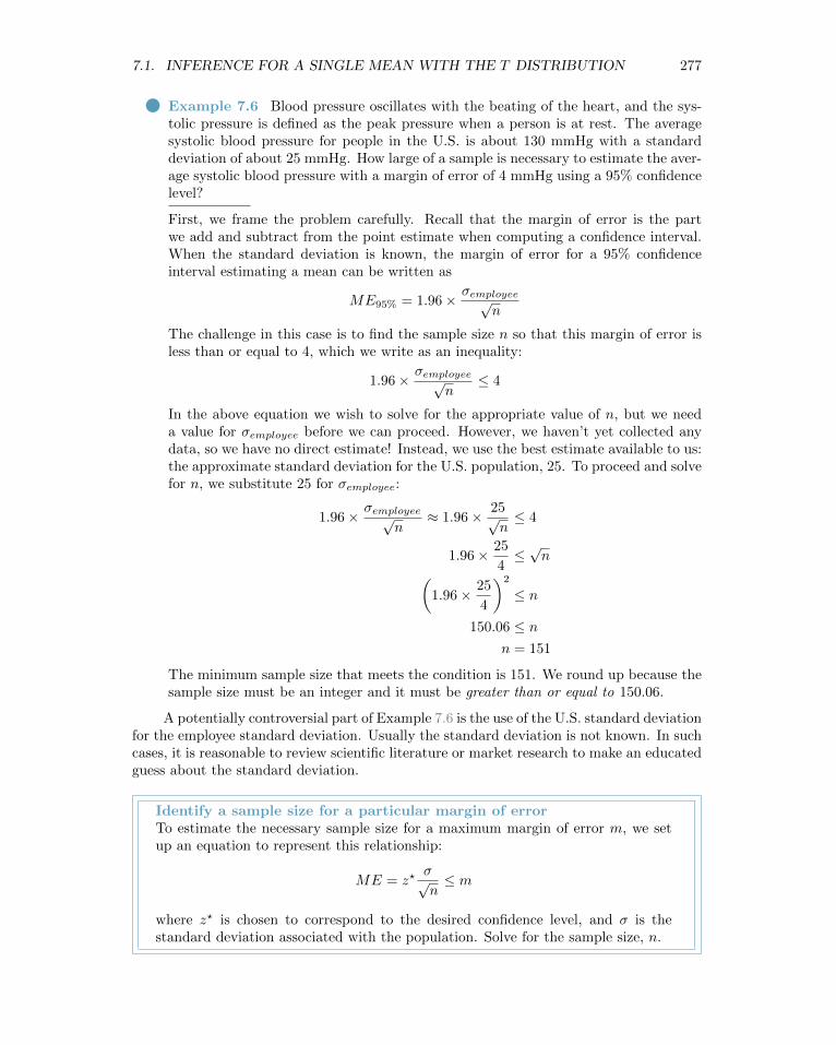
Example 7.6 Blood pressure oscillates with the beating of the heart, and the sys-tolic pressure is defined as the peak pressure when a person is at rest. The averagesystolic blood pressure for people in the U.S. is about 130 mmHg with a standarddeviation of about 25 mmHg. How large of a sample is necessary to estimate the aver-age systolic blood pressure with a margin of error of 4 mmHg using a 95% confidencelevel?

First, we frame the problem carefully. Recall that the margin of error is the partwe add and subtract from the point estimate when computing a confidence interval.When the standard deviation is known, the margin of error for a 95% confidenceinterval estimating a mean can be written as

ME95% = 1.96× σemployee√n

The challenge in this case is to find the sample size n so that this margin of error isless than or equal to 4, which we write as an inequality:

1.96× σemployee√n

≤ 4

In the above equation we wish to solve for the appropriate value of n, but we needa value for σemployee before we can proceed. However, we haven’t yet collected anydata, so we have no direct estimate! Instead, we use the best estimate available to us:the approximate standard deviation for the U.S. population, 25. To proceed and solvefor n, we substitute 25 for σemployee:

1.96× σemployee√n

≈ 1.96× 25√n≤ 4

1.96× 25

4≤√n(

1.96× 25

4

)2

≤ n

150.06 ≤ nn = 151

The minimum sample size that meets the condition is 151. We round up because thesample size must be an integer and it must be greater than or equal to 150.06.

A potentially controversial part of Example 7.6 is the use of the U.S. standard deviationfor the employee standard deviation. Usually the standard deviation is not known. In suchcases, it is reasonable to review scientific literature or market research to make an educatedguess about the standard deviation.

Identify a sample size for a particular margin of errorTo estimate the necessary sample size for a maximum margin of error m, we setup an equation to represent this relationship:

ME = z?σ√n≤ m

where z? is chosen to correspond to the desired confidence level, and σ is thestandard deviation associated with the population. Solve for the sample size, n.


Time (minutes)

Fre

quen

cy

60 80 100 120 140

0

5

10

15

20

25

50 60 70 80 90 100 110 120 130 140 150

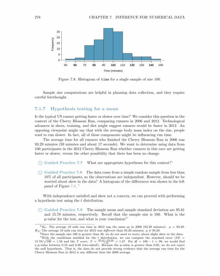
Figure 7.8: Histogram of time for a single sample of size 100.

Sample size computations are helpful in planning data collection, and they requirecareful forethought.

7.1.7 Hypothesis testing for a mean

Is the typical US runner getting faster or slower over time? We consider this question in thecontext of the Cherry Blossom Run, comparing runners in 2006 and 2012. Technologicaladvances in shoes, training, and diet might suggest runners would be faster in 2012. Anopposing viewpoint might say that with the average body mass index on the rise, peopletend to run slower. In fact, all of these components might be influencing run time.

The average time for all runners who finished the Cherry Blossom Run in 2006 was93.29 minutes (93 minutes and about 17 seconds). We want to determine using data from100 participants in the 2012 Cherry Blossom Run whether runners in this race are gettingfaster or slower, versus the other possibility that there has been no change.⊙

Guided Practice 7.7 What are appropriate hypotheses for this context?5

⊙Guided Practice 7.8 The data come from a simple random sample from less than10% of all participants, so the observations are independent. However, should we beworried about skew in the data? A histogram of the differences was shown in the leftpanel of Figure 7.8. 6

With independence satisfied and skew not a concern, we can proceed with performinga hypothesis test using the t distribution.⊙

Guided Practice 7.9 The sample mean and sample standard deviation are 95.61and 15.78 minutes, respectively. Recall that the sample size is 100. What is thep-value for the test, and what is your conclusion?7

5H0: The average 10 mile run time in 2012 was the same as in 2006 (93.29 minutes). µ = 93.29.HA: The average 10 mile run time for 2012 was different than 93.29 minutes. µ 6= 93.29.

6Since the sample size 100 is greater than 30, we do not need to worry about slight skew in the data.7With the conditions satisfied for the t distribution, we can compute the standard error (SE =

15.78/√

100 = 1.58 and the T score: T = 95.61−93.291.58

= 1.47. For df = 100 − 1 = 99, we would finda p-value between 0.10 and 0.20 (two-sided!). Because the p-value is greater than 0.05, we do not rejectthe null hypothesis. That is, the data do not provide strong evidence that the average run time for theCherry Blossom Run in 2012 is any different than the 2006 average.


Hypothesis test for a mean

1. State the name of the test being used: 1-sample t test.

2. Verify conditions.

• Data come from a simple random sample.

• Population is known to be normal OR n ≥ 30 OR graph of data isapproximately symmetric with no outliers, making the assumption thatpopulation is normal a reasonable one.

3. Write the hypotheses in plain language, then set them up in mathematicalnotation.

• H0 : µ = µ0

• H0 : µ 6= or < or > µ0

4. Identify the significance level α.

5. Calculate the test statistic and df .

t =point estimate− null value

SE of estimate

The point estimate is x̄, SE = s√n

, and df = n− 1.

6. Find the p-value, compare it to α, and state whether to reject or not rejectthe null hypothesis.

7. Write your conclusion.

⊙Guided Practice 7.10 Recall the example about the mercury content in croakerwhite fish (Pacific). Based on a sample of 15, a sample mean and standard deviationwere computed as 0.287 and 0.069 ppm (parts per million), respectively. Carry outan appropriate test to determine 0.25 is a reasonable value for the average mercurycontent.8

Example 7.11 Recall that the 95% confidence interval for the average mercuycontent in croaker white fish was (0.249, 0.325). Discuss whether the conclusion of thetest of hypothesis is consistent or inconsistent with the conclusion of the hypothesistest.

It is consistent because 0.25 is located (just barely) inside the confidence interval,so it is a reasonable value. Our hypothesis test did not reject the hypothesis thatµ = 0.25, implying that it is a plausible value. Note, though, that the hypothesis testdid not prove that µ = .25. A hypothesis cannot prove that the mean is a specificvalue. It can only find evidence that it is not a specific value. Note also that thep-value was close to the cutoff of 0.05. This is because the value 0.25 was close toedge of the confidence interval.

8We should carry out a 1-sample t test. The conditions have already been checked. H0 : µ = 0.25;The true average mercury content is 0.25 ppm. HA : µ 6= 0.25; The true average mercury content is notequal to 0.25 ppm. Let α = 0.05. SE = 0.069√

15= 0.0178. t = 0.287−0.25

0.0178= 2.07 df = 15 − 1 = 14.

p-value= 0.057 > 0.05, so we do not reject the null hypothesis. We do not have sufficient evidence that theaverage mercury content in croaker white fish is not 0.25.

5 Foundation for inference

5.1 (a) Mean. Each student reports a numerical value: a number of hours. (b) Mean. Each studentreports a number, which is a percentage, and we can average over these percentages. (c)Proportion. Each student reports Yes or No, so this is a categorical variable and we use aproportion. (d) Mean. Each student reports a number, which is a percentage like in part (b). (e)Proportion. Each student reports whether or not he got a job, so this is a categorical variable andwe use a proportion.

5.3 (a) Mean: 13.65. Median: 14. (b) SD: 1.91. IQR: 15 − 13 = 2. (c) Z16 = 1.23, which is notunusual since it is within 2 SD of the mean. Z18 = 2.23, which is generally considered unusual. (d) No. Point estimates that are based on samples only approximate the population parameter, and they vary from one sample to another. (e) We use the SE, which is

o1.91/

√100 = 0.191 for this sample’s mean.

5.5 Recall that the general formula is

point estimate± z? × SE

First, identify the three different values. The point estimate is 45%, z? = 1.96 for a 95% confidence level, and SE = 1.2%. Then, plug the values into the formula:

45%± 1.96× 1.2% → (42.6%, 47.4%)

Appendix A

End of chapter exercisesolutions

We are 95% confident that the proportion of US adults who live with one or more chronic condi-tions is between 42.6% and 47.4%.

5.7 (a) False. Confidence intervals provide a range of plausible values, and sometimes the truth ismissed. A 95% confidence interval “misses” about 5% of the time. (b) True. Notice that thedescription focuses on the true population value. (c) True. If we examine the 95% confidenceinterval computed in Exercise 5.5, we can see that 50% is not included in this interval. This meansthat in a hypothesis test, we would reject the null hypothesis that the proportion is 0.5. (d) False.The standard error describes the uncertainty in the overall estimate from natural fluctuations dueto randomness, not the uncertainty corresponding to individuals’ responses.

5.9 The subscript pr corresponds to provoca- tive and con to conservative. (a) H0 : ppr = pcon. HA :

ppr 6= pcon. (b) -0.35. (c) The left tail for the p-value is calculated by adding up the two left bins:0.005 + 0.015 = 0.02. Doubling the one tail, the p-value is 0.04. (Students may have approximateresults, and a small number of students may have a p-value of about 0.05.) Since the p-value is low,we reject H0. The data provide strong evidence that people react differ- ently under the twoscenarios.

5.11 The primary concern is confirmation bias. If researchers look only for what they suspect to betrue using a one-sided test, then they are for- mally excluding from consideration the possibil- itythat the opposite result is true. Additionally, if other researchers believe the opposite possibility might be true, they would be very skeptical of the one-sided test.

305.13 (a) H0 : p = 0.69. HA : p 6= 0.69. (b) pˆ = 17 = 0.57. (c) The success-failure condition is not satisfied; note that it is appropriate to use the null value (p0 = 0.69) to compute the expectednumber of successes and failures. (d) Answers may vary. Each student can be represented with acard. Take 100 cards, 69 black cards representing those who follow the news about Egypt and 31 redcards representing those who do not. Shuffle the cards and draw with replacement (shuffling eachtime in between draws) 30 cards representing the 30 high school students. Calculate the proportionof black cards in this sample, pˆsim, i.e. the proportion of those who follow the news in the sim-ulation. Repeat this many times (e.g. 10,000 times) and plot the resulting sample proportions. The

p-value will be two times the proportion of simulations where pˆsim ≤ 0.57. (Note: we wouldgenerally use a computer to perform these simulations.) (e) The p-value is about 0.001 + 0.005 +0.020 + 0.035 + 0.075 = 0.136, meaning the two-sided p-value is about 0.272. Your p-value mayvary slightly since it is based on a visual estimate. Since the p-value is greater than 0.05, we fail toreject H0. The data do not provide strong evidence that the proportion of high school students whofollowed the news about Egypt is different than the proportion of American adults who did.

APPENDIX A. END OF CHAPTER EXERCISE SOLUTIONS

7 Inference for numerical data

?57.1 (a) df = 6 − 1 = 5, t = 2.02 (column with two tails of 0.10, row with df = 5). (b) df = 21 − 1

= 5, t?20 = 2.53 (column with two tails of 0.02, row with df = 20). (c) df = 28, t?28 = 2.05. (d) df = 11, t?11 = 3.11.

7.3 The mean is the midpoint: x¯ = 20. Identify the margin of error: ME = 1.015, then use t*35 = 2.03 and SE = s/

√n in the formula for margin of error to identify s = 3.

7.5 (a) H0: µ = 8 (New Yorkers sleep 8 hrs per night on average.) HA: µ < 8 (New York- ers sleep less than 8 hrs per night on average.) (b) Independence: The sample is random and from less than 10% of New Yorkers. The sample is small, so we will use a t distribution. For this size sample, slight skew is acceptable, and the min/max suggest there is not much skew in the data. T = −1.75. df = 25 − 1 = 24. (c) 0.025 < p-value < 0.05. If in fact the true population mean of the amount New Yorkers sleep per night was 8 hours, the probability of getting a random sample of 25 New Yorkers where the average amount of sleep is 7.73 hrs per night or less is between 0.025 and 0.05. (d) Since p-value < 0.05, reject H0. The data provide strong evidence that New Yorkers sleep less than 8 hours per night on average. (e) No, as we rejected H0.

7.7 t?19 is 1.73 for a one-tail. We want the lower tail, so set -1.73 equal to the T score, then solve for x¯: 56.91.

7.9 (a) For each observation in one data set, there is exactly one specially-corresponding observation in the other data set for the same geo- graphic location. The data are paired. (b) H0 : µdif

f = 0 (There is no difference in average daily high temperature between January 1, 1968 and January 1, 2008 in the continental US.) HA : µdif f > 0 (Average daily high temperature in January 1, 1968 was lower than average daily high temperature in January, 2008 in the continental US.) If you chose a two-sided test, that would also be acceptable. If this is the case, note that your p-value will be a little bigger than what is reported here in part (d). (c) Indepen- dence: locations are random and represent less than 10% of all possible locations in the US. The sample size is at least 30. We are not given the distribution to check the skew. In practice, we would ask to see the data to check this condition, but here we will move forward under the assumption that it is not strongly skewed. (d) Z = 1.60 → p-value = 0.0548. (e) Since the p-value > α (since not given use 0.05), fail to reject H0. The data do not provide strong evidence of temperature warming in the continental US. However it should be noted that the p-value is very close to 0.05. (f) Type 2, since we may have incorrectly failed to reject H0. There may be an increase, but we were unable to detect it. (g) Yes, since we failed to reject H0, which had a null value of 0.

7.11 (a) (-0.03, 2.23). (b) We are 90% confident that the average daily high on January 1, 2008 in the continental US was 0.03 degrees lower to 2.23 degrees higher than the average daily high on January 1, 1968. (c) No, since 0 is included in the interval.

Foundation for inference FOR INFERENCE The sample proportion ^p= 0:15 is called a point estimate of...

Documents

Transcript of Foundation for inference FOR INFERENCE The sample proportion ^p= 0:15 is called a point estimate of...