FORWARD AND BACKWARD FUZZY ECONOMIC ORDER...

FORWARD AND BACKWARD FUZZY ECONOMIC ORDER QUANTITY MODELS CONSIDERING LEARNING

THEORY

EHSAN SHEKARIAN

FACULTY OF ENGINEERING UNIVERSITY OF MALAYA

KUALA LUMPUR

2017

FORWARD AND BACKWARD FUZZY ECONOMIC

ORDER QUANTITY MODELS CONSIDERING

LEARNING THEORY

EHSAN SHEKARIAN

THESIS SUBMITTED IN FULFILMENT OF THE

REQUIREMENTS FOR THE DEGREE OF DOCTOR OF

PHILOSOPHY

FACULTY OF ENGINEERING

UNIVERSITY OF MALAYA

KUALA LUMPUR

2017

ii

UNIVERSITY OF MALAYA

ORIGINAL LITERARY WORK DECLARATION

Name of Candidate: Ehsan Shekarian I.C/Passport No: E96015940

Registration/Matric No: KHA130125

Name of Degree: Doctor of Philosophy

Title of Thesis:

Forward and Backward Fuzzy Economic Order Quantity Models Considering

Learning Theory

Field of Study: Manufacturing Management (Engineering and Engineering Trades)

I do solemnly and sincerely declare that:

(1) I am the sole author/writer of this Work;

(2) This Work is original;

(3) Any use of any work in which copyright exists was done by way of fair dealing

and for permitted purposes and any excerpt or extract from, or reference to or

reproduction of any copyright work has been disclosed expressly and

sufficiently and the title of the Work and its authorship have been

acknowledged in this Work;

(4) I do not have any actual knowledge nor do I ought reasonably to know that the

making of this work constitutes an infringement of any copyright work;

(5) I hereby assign all and every rights in the copyright to this Work to the

University of Malaya (“UM”), who henceforth shall be owner of the copyright

in this Work and that any reproduction or use in any form or by any means

whatsoever is prohibited without the written consent of UM having been first

had and obtained;

(6) I am fully aware that if in the course of making this Work I have infringed any

copyright whether intentionally or otherwise, I may be subject to legal action

or any other action as may be determined by UM.

Candidate’s Signature Date: 15/03/2017

Ehsan Shekarian

Subscribed and solemnly declared before,

Witness’s Signature Date:

Name:

Designation:

Safri

Highlight

iii

UNIVERSITI MALAYA

PERAKUAN KEASLIAN PENULISAN

Nama: Ehsan Shekarian No. K.P/Pasport: E96015940

No. Pendaftaran/Matrik: KHA130125

Nama Ijazah: Doctor of Philosophy

Tajuk Tesis:

Forward and Backward Fuzzy Economic Order Quantity Models Considering

Learning Theory

Bidang Penyelidikan: Manufacturing Management

(Engineering and Engineering Trades)

Saya dengan sesungguhnya dan sebenarnya mengaku bahawa:

(1) Saya adalah satu-satunya pengarang/penulis Hasil Kerja ini;

(2) Hasil Kerja ini adalah asli;

(3) Apa-apa penggunaan mana-mana hasil kerja yang mengandungi hakcipta telah

dilakukan secara urusan yang wajar dan bagi maksud yang dibenarkan dan apa-

apa petikan, ekstrak, rujukan atau pengeluaran semula daripada atau kepada

mana-mana hasil kerja yang mengandungi hakcipta telah dinyatakan dengan

sejelasnya dan secukupnya dan satu pengiktirafan tajuk hasil kerja tersebut dan

pengarang/penulisnya telah dilakukan di dalam Hasil Kerja ini;

(4) Saya tidak mempunyai apa-apa pengetahuan sebenar atau patut

semunasabahnya tahu bahawa penghasilan Hasil Kerja ini melanggar suatu

hakcipta hasil kerja yang lain;

(5) Saya dengan ini menyerahkan kesemua dan tiap-tiap hak yang terkandung di

dalam hakcipta Hasil Kerja ini kepada Universiti Malaya (“UM”) yang

seterusnya mula dari sekarang adalah tuan punya kepada hakcipta di dalam

Hasil Kerja ini dan apa-apa pengeluaran semula atau penggunaan dalam apa

jua bentuk atau dengan apa juga cara sekalipun adalah dilarang tanpa terlebih

dahulu mendapat kebenaran bertulis dari UM;

(6) Saya sedar sepenuhnya sekiranya dalam masa penghasilan Hasil Kerja ini saya

telah melanggar suatu hakcipta hasil kerja yang lain sama ada dengan niat atau

sebaliknya, saya boleh dikenakan tindakan undang-undang atau apa-apa

tindakan lain sebagaimana yang diputuskan oleh UM.

Tandatangan Calon Tarikh: 15/03/2017

Ehsan Shekarian

Diperbuat dan sesungguhnya diakui di hadapan,

Tandatangan Saksi Tarikh:

Nama:

Jawatan:

Safri

Highlight

iv

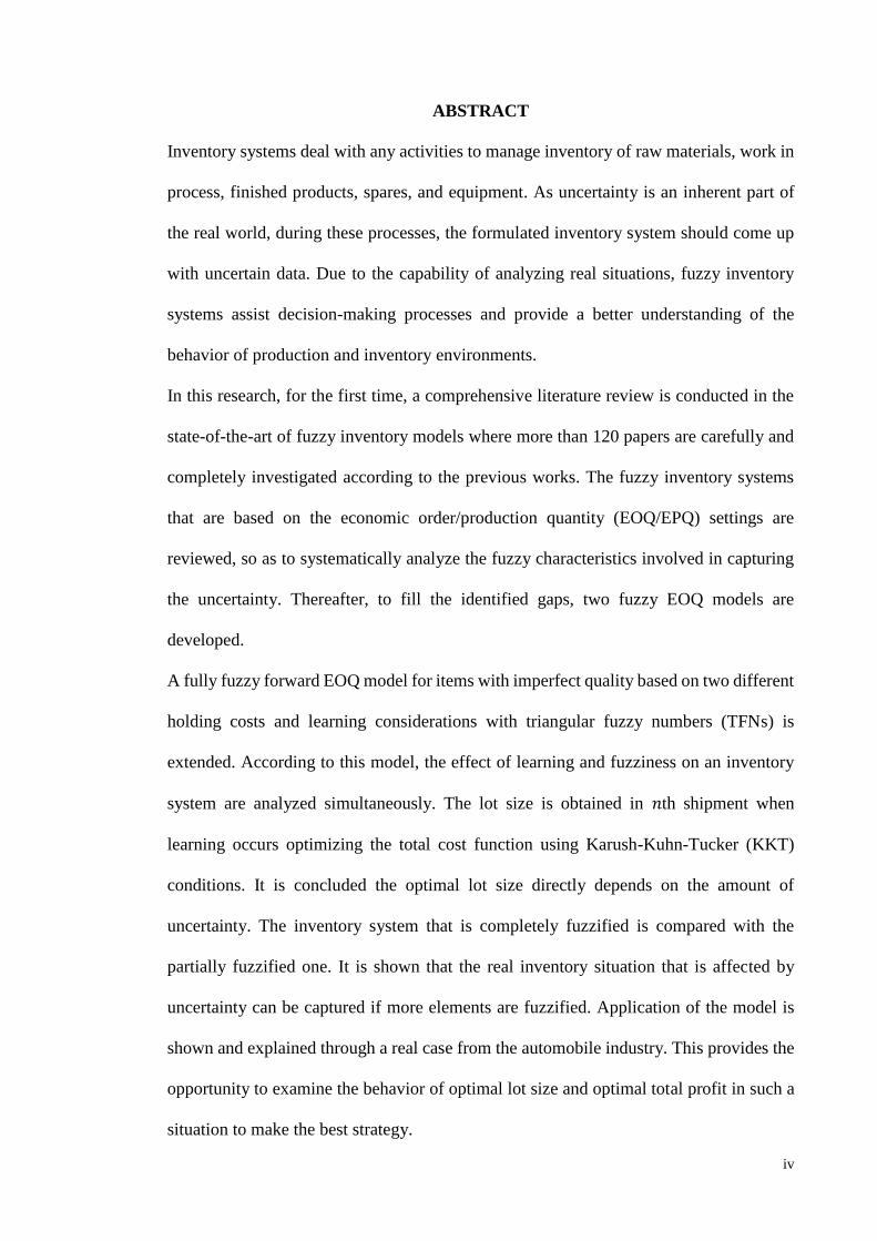
ABSTRACT

Inventory systems deal with any activities to manage inventory of raw materials, work in

process, finished products, spares, and equipment. As uncertainty is an inherent part of

the real world, during these processes, the formulated inventory system should come up

with uncertain data. Due to the capability of analyzing real situations, fuzzy inventory

systems assist decision-making processes and provide a better understanding of the

behavior of production and inventory environments.

In this research, for the first time, a comprehensive literature review is conducted in the

state-of-the-art of fuzzy inventory models where more than 120 papers are carefully and

completely investigated according to the previous works. The fuzzy inventory systems

that are based on the economic order/production quantity (EOQ/EPQ) settings are

reviewed, so as to systematically analyze the fuzzy characteristics involved in capturing

the uncertainty. Thereafter, to fill the identified gaps, two fuzzy EOQ models are

developed.

A fully fuzzy forward EOQ model for items with imperfect quality based on two different

holding costs and learning considerations with triangular fuzzy numbers (TFNs) is

extended. According to this model, the effect of learning and fuzziness on an inventory

system are analyzed simultaneously. The lot size is obtained in 𝑛th shipment when

learning occurs optimizing the total cost function using Karush-Kuhn-Tucker (KKT)

conditions. It is concluded the optimal lot size directly depends on the amount of

uncertainty. The inventory system that is completely fuzzified is compared with the

partially fuzzified one. It is shown that the real inventory situation that is affected by

uncertainty can be captured if more elements are fuzzified. Application of the model is

shown and explained through a real case from the automobile industry. This provides the

opportunity to examine the behavior of optimal lot size and optimal total profit in such a

situation to make the best strategy.

v

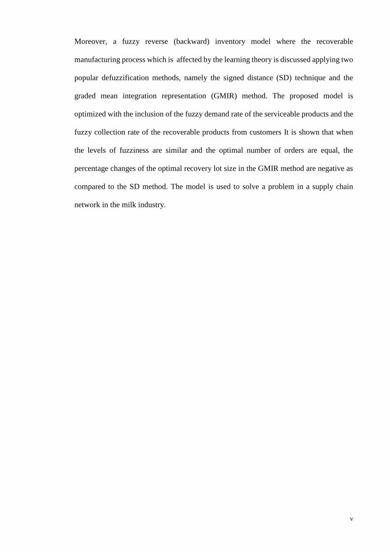
Moreover, a fuzzy reverse (backward) inventory model where the recoverable

manufacturing process which is affected by the learning theory is discussed applying two

popular defuzzification methods, namely the signed distance (SD) technique and the

graded mean integration representation (GMIR) method. The proposed model is

optimized with the inclusion of the fuzzy demand rate of the serviceable products and the

fuzzy collection rate of the recoverable products from customers It is shown that when

the levels of fuzziness are similar and the optimal number of orders are equal, the

percentage changes of the optimal recovery lot size in the GMIR method are negative as

compared to the SD method. The model is used to solve a problem in a supply chain

network in the milk industry.

vi

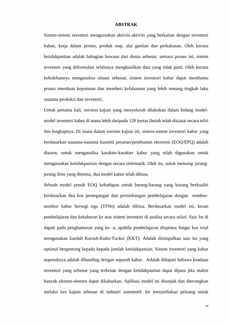
ABSTRAK

Sistem-sistem inventori menguruskan aktiviti-aktiviti yang berkaitan dengan inventori

bahan, kerja dalam proses, produk siap, alat gantian dan perkakasan. Oleh kerana

ketidakpastian adalah bahagian bawaan dari dunia sebenar, semasa proses ini, sistem

inventori yang diformulasi selalunya menghasilkan data yang tidak pasti. Oleh kerana

kebolehannya menganalisa situasi sebenar, sistem inventori kabur dapat membantu

proses membuat keputusan dan memberi kefahaman yang lebih tentang tingkah laku

suasana produksi dan inventori.

Untuk pertama kali, soroton kajian yang menyeluruh dilakukan dalam bidang model-

model inventori kabur di mana lebih daripada 120 kertas ilmiah telah disiasat secara teliti

dan lengkapnya. Di mana dalam sorotan kajian ini, sistem-sistem inventori kabur yang

berdasarkan suasana-suasana kuantiti pesanan/pembuatan ekonomi (EOQ/EPQ) adalah

disorot, untuk menganalisa karakter-karakter kabur yang telah digunakan untuk

menguruskan ketidakpastian dengan secara sistematik. Oleh itu, untuk menutup jurang-

jurang ilmu yang ditemui, dua model kabur telah dibina.

Sebuah model penuh EOQ kehadapan untuk barang-barang yang kurang berkualiti

berdasarkan dua kos pemegangan dan pertimbangan pembelajaran dengan nombor-

nombor kabur bersegi tiga (TFNs) adalah dibina. Berdasarkan model ini, kesan

pembelajaran dan kekaburan ke atas sistem inventori di analisa secara selari. Saiz lot di

dapati pada penghantaran yang ke- n, apabila pembelajaran dioptima fungsi kos total

mengunakan kaedah Karush-Kuhn-Tucker (KKT). Adalah disimpulkan saiz lot yang

optimal bergantung kepada kepada jumlah ketidakpastian. Sistem inventori yang kabur

sepenuhnya adalah dibanding dengan separuh kabur. Adalah didapati bahawa keadaan

inventori yang sebenar yang terkesan dengan ketidakpastian dapat dijana jika makin

banyak elemen-elemen dapat dikaburkan. Aplikasi model ini ditunjuk dan diterangkan

melalui kes kajian sebenar di industri automotif. Ini menyediakan peluang untuk

vii

mengkaji tingkah laku saiz lot optimal dan keuntungan total optimal dalam keadaan

terbaik untuk membuat keputusan.

Tambahan pula, model inventori kabur balikan dimana proses pembuatan terkembalikan

yang terkesan oleh teori pembelajaran adalah dibincangkan- mengaplikasikan dua kaedah

pengeyahkaburan, iaitu teknik “signed distance” (SD) dan “graded mean integration

representation” (GMIR). Model yang dicadangkan ini adalah dioptima dengan

mengambil kira kadar pemintaan kabur bagi produk-produk yang boleh diservis dan

kadar kutipan kabur dari produk-produk yang boleh-dikembalikan dari pelanggan.

Ditunjukkan apabila takat-takat kekaburan adalah sama dan bilangan permintaan yang

optimal adalah sama, kadar perubahan peratusan bagi saiz lot terkembalikan yang optimal

dengan kaedah GMIR adalah negatif berbanding dengan kaedah SD. Model ini digunakan

untuk menyelesaikan masalah rangkai rantaian bekalan di industry tenusu.

viii

ACKNOWLEDGEMENTS

I would like to give all glory to the almighty God for providing me the opportunity,

patience and aptitude to accomplish this work. He has been the source of hope and

strength in my life and has granted me with countless benevolent gifts.

I would like to express deep gratitude to my supervisors Dr. Ezutah Udoncy Olugu and

Dr. Salwa Hanim Binti Abdul-Rashid, for all their benign guidance and invaluable

support during this research, and for having faith in me to be able to achieve this

accomplishment.

My appreciation goes as well to Dr. Raja Ariffin Raja Ghazilla as Internal Examiner, and

Professor Dr. Alvin Culaba and Professor Dr. Madjid Tavana as External Examiners, for

their insightful and constructive comments and suggestions.

I would also like to extend my appreciation to staffs of Centre for Product Design and

Manufacturing, and Faculty of Mechanical Engineering, University of Malaya, Kuala

Lumpur, Malaysia for their kind assistance rendered to me throughout my study. My

gratitude also goes to Institute of Research Management & Monitoring (IPPP) of

University of Malaya for their financial support.

Lastly but not the least, I tend to take this opportunity to thank my beloved parents, my

brothers, and sister for supporting me spiritually throughout writing this thesis and my life in

general.

ix

TABLE OF CONTENTS

Abstract ........................................................................................................................... ivi

Abstrak ............................................................................................................................. vi

Acknowledgements ........................................................................................................ viii

Table of Contents ............................................................................................................. ix

List of Figures ................................................................................................................. xv

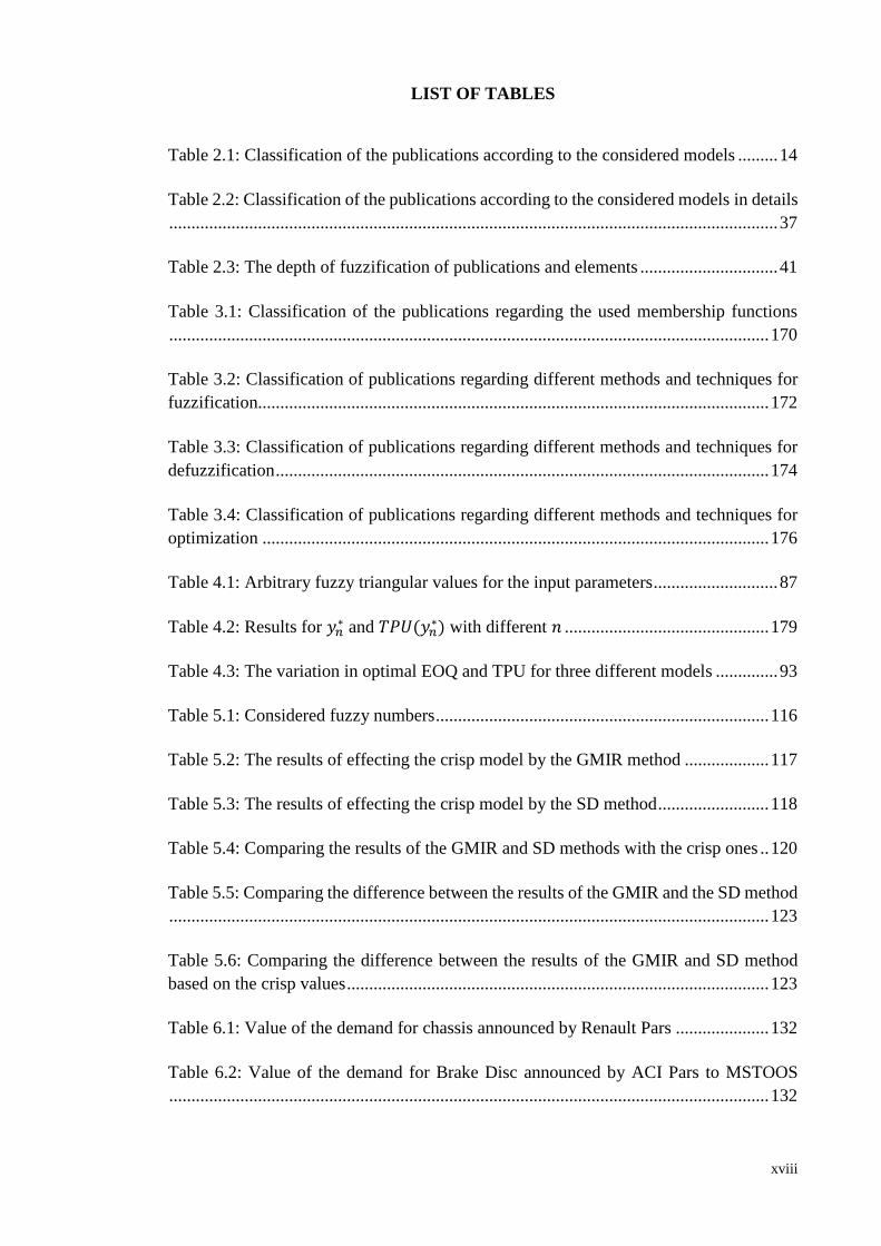
List of Tables................................................................................................................ xviii

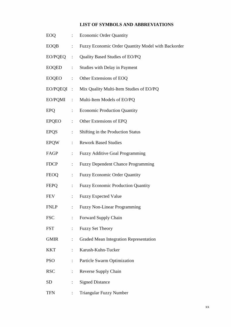
List of Symbols and Abbreviations ................................................................................. xx

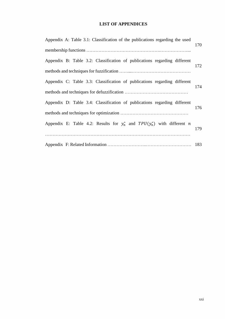
List of Appendices ......................................................................................................... xxi

CHAPTER 1: INTRODUCTION .................................................................................. 1

1.1 Research Background .............................................................................................. 1

1.2 Research Gaps ........................................................................................................ 2

1.3 Problem Statement ................................................................................................... 3

1.4 Aim and Objectives ................................................................................................ 4

1.5 Research Questions .................................................................................................. 5

1.6 Research Framework ............................................................................................... 5

1.7 Thesis Layout........................................................................................................... 7

CHAPTER 2: LITERATURE REVIEW ...................................................................... 8

2.1 Introduction.............................................................................................................. 8

2.2 Inventory Management ............................................................................................ 8

2.3 Fuzzy Set Theory ..................................................................................................... 9

2.4 Fuzzy Inventory Management ................................................................................. 9

2.5 Methodology of Literature Review ....................................................................... 11

2.5.1 Material Collection ................................................................................... 11

2.5.2 Descriptive Analysis ................................................................................. 12

x

2.5.3 Category Selection .................................................................................. 12

2.5.4 Material Evaluation ................................................................................. 15

2.6 Economic Order Quantity Model ......................................................................... 16

2.6.1 Fuzzy Economic Order Quantity Model ................................................. 16

2.6.1.1 Fuzzy Economic Order Quantity Model without Backorder

(EOQ) ........................................................................................ 17

2.6.1.2 Fuzzy Economic Order Quantity Model with Backorder (EOQB)

........................................................................................ 18

2.6.1.3 Extensions Fuzzy Economic Order Quantity Model ................. 20

(a) Quality Based Studies (EOQEQ) ......................................... 20

(b) Multi-Item Models (EOQMI) ............................................... 21

(c) Mix Quality Multi-Item Studies (EOQEQI) ......................... 23

(d) Studies with Delay in Payment (EOQED) ........................... 24

(e) Other Extensions of EOQ (EOQEO) ................................... 26

2.7 Economic Production Quantity Model ................................................................. 28

2.7.1 Fuzzy Economic Production Quantity Model ......................................... 28

2.7.1.1 Fuzzy Basic Economic Production Quantity Model (EPQ) ...... 28

2.7.1.2 Extensions Fuzzy Economic Production Quantity Model......... 29

(a) Quality Based Studies (EPQEQ) ......................................... 29

(b) Rework based Studies (EPQW) ............................................ 30

(c) Shifting in the Production Status (EPQS) ............................ 31

(d) Multi-Item Studies (EPQEQI) .............................................. 32

(e) Mix Quality Multi-Item Studies (EPQEQI) .......................... 33

(f) Other Extensions of EPQ (EPQEO) ..................................... 34

2.8 Fuzzified Elements and Characteristics ................................................................. 35

2.9 Chapter Summary .................................................................................................. 36

xi

CHAPTER 3: METHODOLOGY ............................................................................... 49

3.1 Introduction............................................................................................................ 49

3.2 Research Methodology .......................................................................................... 49

3.3 Research Framework in Details ............................................................................. 51

3.4 Fuzzification Process ............................................................................................. 52

3.4.1 Preliminaries and Fundamental Definitions ............................................. 52

3.4.2 Generalized Fuzzy Numbers .................................................................... 54

3.4.3 Overview of the Previous Fuzzy Numbers ............................................... 54

3.4.4 Justification of the Triangular Fuzzy Number ......................................... 55

3.4.5 Overview of the Previous Fuzzification Methods .................................... 56

3.4.6 Fuzzy Arithmetic ...................................................................................... 56

3.4.7 Principle of Decomposition Theory ......................................................... 59

3.4.8 Justification of the Function Principle Methods ....................................... 60

3.5 Defuzzification Process ......................................................................................... 61

3.5.1 Overview of the Previous Defuzzification Methods ................................ 61

3.5.1.1 GMIR Method ........................................................................... 61

3.5.1.2 Graded Mean Integration Representation of TFN ..................... 62

3.5.1.3 Signed Distance Method ........................................................... 63

3.5.2 Justification of the GMIR and SD methods ............................................. 65

3.6 Optimization Methods ........................................................................................... 65

3.6.1 Overview of the Previous Optimization Methods .................................... 66

3.6.2 KKT Method ............................................................................................ 66

3.6.3 Intermediate Value Theorem .................................................................... 67

3.7 Characteristics of the Developed Models .............................................................. 67

3.7.1 Learning Theory ....................................................................................... 67

3.7.2 Imperfect Quality Items ............................................................................ 70

xii

3.7.3 Holding Cost ............................................................................................. 70

3.7.4 Return Process .......................................................................................... 70

3.8 Chapter Summary .................................................................................................. 71

CHAPTER 4: FULLY FUZZY FORWARD ECONOMIC ORDER QUANTITY

MODEL CONSIDERING LEARNING EFFECTS .................................................. 72

4.1 Introduction............................................................................................................ 72

4.2 Problem Description .............................................................................................. 72

4.2.1 Assumptions ............................................................................................. 73

4.2.2 Notations .................................................................................................. 73

4.3 Model Formulation ................................................................................................ 74

4.4 Fully Fuzzy Model ................................................................................................. 77

4.5 Finding Optimal Values ......................................................................................... 83

4.6 Numerical Illustrations .......................................................................................... 86

4.7 Comparing to the Earlier Models .......................................................................... 90

4.8 Managerial Insight ................................................................................................. 93

4.9 Chapter Summary .................................................................................................. 94

CHAPTER 5: FUZZY BACKWARD ECONOMIC ORDER/PRODUCTION

QUANTITY MODEL WITH LEARNING ................................................................ 96

5.1 Introduction............................................................................................................ 96

5.2 Problem Description .............................................................................................. 96

5.2.1 Assumptions ............................................................................................. 97

5.2.2 Notations .................................................................................................. 97

5.3 Reverse Model Formulation .................................................................................. 98

5.4 Fuzzy Reverse Inventory Model .......................................................................... 102

5.4.1 Defuzzification by the SD Method ......................................................... 103

5.4.2 Finding the Optimal Values for the SD Method .................................... 107

xiii

5.4.3 Defuzzification by the GMIR Method ................................................... 109

5.4.4 Finding the Optimal Values for the GMIR Method ............................... 111

5.5 Solution Procedure............................................................................................... 114

5.6 One-dimensional Search Procedure for Optimization ......................................... 114

5.7 Comprehensive Numerical Example ................................................................... 115

5.8 Chapter Summary ................................................................................................ 125

CHAPTER 6: APPLICATIONS TO CASE STUDIES ........................................... 127

6.1 Introduction.......................................................................................................... 127

6.2 First Case Study ................................................................................................... 127

6.2.1 A Supply Chain in an Automobile Industry ........................................... 127

6.2.2 Gathering the Information ...................................................................... 129

6.2.3 Adapting to the First Fuzzy Model ....................................................... 135

6.2.4 Calculations ............................................................................................ 136

6.2.5 Analyzing the Results ............................................................................. 139

6.3 Second Case Study .............................................................................................. 140

6.3.1 Milk Manufacturing Company ............................................................... 140

6.3.2 Polyethylene Terephthalate (PET) ......................................................... 141

6.3.3 Milk Supply Chain Network .................................................................. 141

6.3.4 Related Information to Adapt the Second Fuzzy Model ........................ 143

6.3.5 Calculations ............................................................................................ 144

6.3.6 Analyzing the Results ............................................................................. 147

6.3 Chapter Summary ................................................................................................ 148

CHAPTER 7: CONCLUSION ................................................................................... 149

7.1 Concluding Remarks ........................................................................................... 149

7.2 Contributions and Applications ........................................................................... 152

7.2.1 Contribution to the Knowledge .............................................................. 152

xiv

7.2.2 Contribution to the Practitioners ............................................................ 153

7.3 Recommendations for Future Research ............................................................... 154

References ..................................................................................................................... 156

List of Publications and Papers Presented .................................................................... 169

Appendix ....................................................................................................................... 170

xv

LIST OF FIGURES

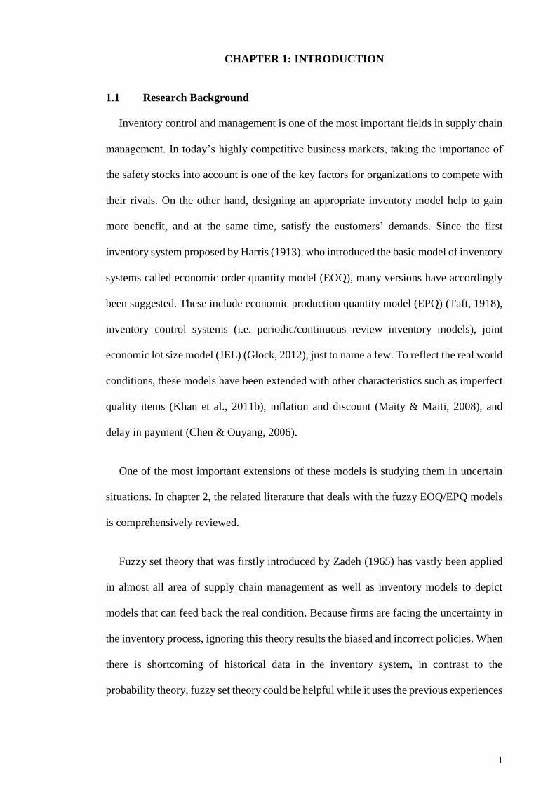
Figure 1.1: Designing of the inventory system ................................................................. 3

Figure 1.2: Research framework ....................................................................................... 6

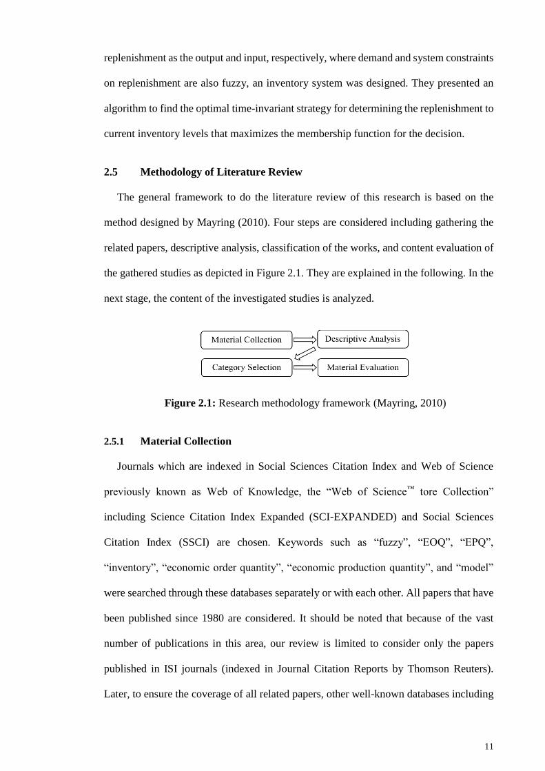
Figure 2.1: Research methodology framework (Mayring, 2010) ................................... 11

Figure 2.2: Distribution of the published papers per year over the investigated time

interval............................................................................................................................. 11

Figure 2.3: Distribution of publications based on different journals .............................. 11

Figure 3.1: Research methodology ................................................................................. 51

Figure 3.2: Details of research framework ...................................................................... 52

Figure 3.3: Triangular fuzzy number .............................................................................. 55

Figure 3.4: Addition operation of two fuzzy numbers .................................................... 57

Figure 3.5: Product operation of two fuzzy numbers ...................................................... 58

Figure 3.6: The graded mean α-level value of generalized fuzzy number Β̃ .................. 62

Figure 3.7: Wright’s learning curve ................................................................................ 69

Figure 3.8: The three phases of the learning curve ......................................................... 69

Figure 4.1: Inventory time plot for an EOQ model with imperfect quality .................... 74

Figure 4.2: Three dimensional-graph of optimal order quantity, level of fuzziness and

number of shipments ....................................................................................................... 88

Figure 4.3: Three dimensional-graph of total profit per unit time, level of fuzziness and

number of shipments ....................................................................................................... 89

Figure 4.4: Comparison of the behavior of three different models for EOQ under 10

percent of uncertainty for the first 10 shipments ............................................................ 91



Figure 4.6: Comparison of the behavior of three different models for TPU under 10


xvi



Figure 5.1: Recovery process under the effect of learning ............................................. 97

Figure 5.2: Inventory levels of collected items from customers for 𝑛=2 ........................ 99

Figure 5.3: Inventory levels of serviceable items for 𝑛=2 ............................................ 101

Figure 5.4: Proposed flowchart to find the optimal recovery lot size and the number of

orders ............................................................................................................................. 115

Figure 5.5: Comparing the SD and the GMIR method simultaneously considering the

relative variation between the crisp and fuzzy situation for the optimal recovery lot size

....................................................................................................................................... 121


relative variation between the crisp and fuzzy situation for the optimal total cost function

per unit time .................................................................................................................. 122

Figure 5.7: Estimating a simple regression relationship between the values obtained by

𝑇𝐶𝑈∗𝑆𝐷% and summation of 𝜃1 and 𝜃4. ........................................................................ 124


𝑇𝐶𝑈∗𝐺𝑀𝐼𝑅% and summation of 𝜃1 and 𝜃4.. ................................................................... 124

Figure 6.1: L-90 (Tondar 90).. ...................................................................................... 128

Figure 6.2: Supply chain network of considered automobile industry.. ....................... 128

Figure 6.3: Brake Disc 259*20,6' painted ..................................................................... 129

Figure 6.4: Rear Hub Drum 8' painted .......................................................................... 130

Figure 6.5: Function of the Brake Disc (www.explainthatstuff.com) .......................... 130

Figure 6.6: Function of the Rear Hub Drum (www.auto.howstuffworks.com) ............ 131

Figure 6.7: Steel pallet for screening ............................................................................ 134

Figure 6.8: Optimal order quantity for Brake Disc for 10 and 70 percent level of fuzziness

....................................................................................................................................... 137

Figure 6.9: Total profit per unit time for Brake Disc for 10 and 70 percent level of

fuzziness ........................................................................................................................ 137

xvii

Figure 6.10: Optimal order quantity for Rear Hub Drum for 10 and 70 percent level of

fuzziness ........................................................................................................................ 138

Figure 6.11: Total profit per unit time for Rear Hub Drum for 10 and 70 percent level of

fuzziness ........................................................................................................................ 138

Figure 6.12: Milk supply chain network ....................................................................... 143

Figure 6.13: Comparison of effect of fuzzification of parameters on the number of orders

for the newly purchased items during a cycle in both defuzzification methods ........... 145

Figure 6.14: Comparison of effect of fuzzification of parameters on the recovery lot size

of items for each production run in both defuzzification methods ............................... 145

Figure 6.15: Comparison of effect of fuzzification of parameters on the ordering lot size

for the newly purchased items in both defuzzification methods ................................... 146

Figure 6.16: Comparison of effect of fuzzification of parameters on the total cost function

per unit time in both defuzzification methods............................................................... 146

Figure 6.17: ACI Pars organizational structure ............................................................ 183

Figure 6.18: Production of L-90 by Iran Khodro May and June, 2015 ........................ 184

Figure 6.19: Price of some parts of braking system of L90 ....................................... ...185

Figure 6.20: Production of milk for provinces of Iran .................................................. ...186

xviii

LIST OF TABLES

Table 2.1: Classification of the publications according to the considered models ......... 14

Table 2.2: Classification of the publications according to the considered models in details

......................................................................................................................................... 37

Table 2.3: The depth of fuzzification of publications and elements ............................... 41

Table 3.1: Classification of the publications regarding the used membership functions

....................................................................................................................................... 170

Table 3.2: Classification of publications regarding different methods and techniques for

fuzzification................................................................................................................... 172


defuzzification ............................................................................................................... 174


optimization .................................................................................................................. 176

Table 4.1: Arbitrary fuzzy triangular values for the input parameters ............................ 87

Table 4.2: Results for 𝑦𝑛∗ and 𝑇𝑃𝑈(𝑦𝑛

∗) with different 𝑛 .............................................. 179

Table 4.3: The variation in optimal EOQ and TPU for three different models .............. 93

Table 5.1: Considered fuzzy numbers ........................................................................... 116

Table 5.2: The results of effecting the crisp model by the GMIR method ................... 117

Table 5.3: The results of effecting the crisp model by the SD method ......................... 118

Table 5.4: Comparing the results of the GMIR and SD methods with the crisp ones .. 120

Table 5.5: Comparing the difference between the results of the GMIR and the SD method

....................................................................................................................................... 123

Table 5.6: Comparing the difference between the results of the GMIR and SD method

based on the crisp values ............................................................................................... 123

Table 6.1: Value of the demand for chassis announced by Renault Pars ..................... 132

Table 6.2: Value of the demand for Brake Disc announced by ACI Pars to MSTOOS

....................................................................................................................................... 132

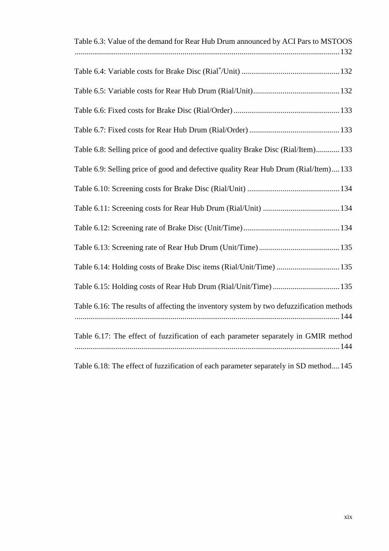
xix

Table 6.3: Value of the demand for Rear Hub Drum announced by ACI Pars to MSTOOS

....................................................................................................................................... 132

Table 6.4: Variable costs for Brake Disc (Rial*/Unit) .................................................. 132

Table 6.5: Variable costs for Rear Hub Drum (Rial/Unit) ............................................ 132

Table 6.6: Fixed costs for Brake Disc (Rial/Order) ...................................................... 133

Table 6.7: Fixed costs for Rear Hub Drum (Rial/Order) .............................................. 133

Table 6.8: Selling price of good and defective quality Brake Disc (Rial/Item) ............ 133

Table 6.9: Selling price of good and defective quality Rear Hub Drum (Rial/Item) .... 133

Table 6.10: Screening costs for Brake Disc (Rial/Unit) ............................................... 134

Table 6.11: Screening costs for Rear Hub Drum (Rial/Unit) ....................................... 134

Table 6.12: Screening rate of Brake Disc (Unit/Time) ................................................. 134

Table 6.13: Screening rate of Rear Hub Drum (Unit/Time) ......................................... 135

Table 6.14: Holding costs of Brake Disc items (Rial/Unit/Time) ................................ 135

Table 6.15: Holding costs of Rear Hub Drum (Rial/Unit/Time) .................................. 135

Table 6.16: The results of affecting the inventory system by two defuzzification methods

....................................................................................................................................... 144

Table 6.17: The effect of fuzzification of each parameter separately in GMIR method

....................................................................................................................................... 144

Table 6.18: The effect of fuzzification of each parameter separately in SD method .... 145

xx

LIST OF SYMBOLS AND ABBREVIATIONS

EOQ : Economic Order Quantity

EOQB : Fuzzy Economic Order Quantity Model with Backorder

EO/PQEQ : Quality Based Studies of EO/PQ

EOQED : Studies with Delay in Payment

EOQEO : Other Extensions of EOQ

EO/PQEQI : Mix Quality Multi-Item Studies of EO/PQ

EO/PQMI : Multi-Item Models of EO/PQ

EPQ : Economic Production Quantity

EPQEO : Other Extensions of EPQ

EPQS : Shifting in the Production Status

EPQW : Rework Based Studies

FAGP : Fuzzy Additive Goal Programming

FDCP : Fuzzy Dependent Chance Programming

FEOQ : Fuzzy Economic Order Quantity

FEPQ : Fuzzy Economic Production Quantity

FEV : Fuzzy Expected Value

FNLP : Fuzzy Non-Linear Programming

FSC : Forward Supply Chain

FST : Fuzzy Set Theory

GMIR : Graded Mean Integration Representation

KKT : Karush-Kuhn-Tucker

PSO : Particle Swarm Optimization

RSC : Reverse Supply Chain

SD : Signed Distance

TFN : Triangular Fuzzy Number

xxi

LIST OF APPENDICES

Appendix A: Table 3.1: Classification of the publications regarding the used

membership functions ………………………………………….………………...

170

Appendix B: Table 3.2: Classification of publications regarding different

methods and techniques for fuzzification ……...…………………………………

172

Appendix C: Table 3.3: Classification of publications regarding different

methods and techniques for defuzzification ……………………………………

174

Appendix D: Table 3.4: Classification of publications regarding different

methods and techniques for optimization ………………………………………

176

Appendix E: Table 4.2: Results for 𝑦𝑛∗ and 𝑇𝑃𝑈(𝑦𝑛

∗) with different 𝑛

……………………………………………………………………………………

179

Appendix F: Related Information ……………………..………………………… 183

1

CHAPTER 1: INTRODUCTION

1.1 Research Background

Inventory control and management is one of the most important fields in supply chain

management. In today’s highly competitive business markets, taking the importance of

the safety stocks into account is one of the key factors for organizations to compete with

their rivals. On the other hand, designing an appropriate inventory model help to gain

more benefit, and at the same time, satisfy the customers’ demands. Since the first

inventory system proposed by Harris (1913), who introduced the basic model of inventory

systems called economic order quantity model (EOQ), many versions have accordingly

been suggested. These include economic production quantity model (EPQ) (Taft, 1918),

inventory control systems (i.e. periodic/continuous review inventory models), joint

economic lot size model (JEL) (Glock, 2012), just to name a few. To reflect the real world

conditions, these models have been extended with other characteristics such as imperfect

quality items (Khan et al., 2011b), inflation and discount (Maity & Maiti, 2008), and

delay in payment (Chen & Ouyang, 2006).

One of the most important extensions of these models is studying them in uncertain

situations. In chapter 2, the related literature that deals with the fuzzy EOQ/EPQ models

is comprehensively reviewed.

Fuzzy set theory that was firstly introduced by Zadeh (1965) has vastly been applied

in almost all area of supply chain management as well as inventory models to depict

models that can feed back the real condition. Because firms are facing the uncertainty in

the inventory process, ignoring this theory results the biased and incorrect policies. When

there is shortcoming of historical data in the inventory system, in contrast to the

probability theory, fuzzy set theory could be helpful while it uses the previous experiences

2

of the decision makers and managers. Hence, it is becoming increasingly difficult to

ignore developing inventory models in fuzzy environment.

In this study, inventory models in fuzzy environment regarding some characteristics

for the model which are mainly based on the learning theory and the rate of return of used

products in the inventory systems are tried to be developed. Some policies when these

characteristics are integrated in an uncertain environment are suggested.

1.2 Research Gaps

Although the fuzzy set theory has widely been investigated in inventory models, there

are still a lot of potential rooms for research. One of the research agenda can be studying

the depth of fuzziness of an inventory system. It answers to what will occur if an inventory

system is extended and considered in a forward supply chain (FSC) with a complete

uncertain situation? Usually the previous researches deal with an inventory system in a

partially uncertain condition. It means that they fuzzified the whole of the system to some

special levels. The more the level and the depth of fuzziness, the more complex the system

is. As optimizing the system is very hard in a fully fuzzy environment, researches to date

have tended to focus on fuzzification of a part of the inventory system while the other

part remains as crisp one.

In this study, the behavior of an EOQ system which is completely fuzzy is attempted

to be analyzed. Besides, formulated model includes other characteristics such as learning

process that usually affects inventory systems.

Literature has emerged that most of the related researches have tended to integrate

fuzzy set theory on forward inventory management while using this theory in backward

(reverse) inventory systems is still in its infancy. Moreover, as a reverse cycle occurs in

such systems, the importance of the combination of this system with fuzziness even could

3

be more. In order to design a more effective reverse inventory system through a reverse

supply chain (RSC), this theory undoubtedly is one of the best tools.

In another part of this study, a reverse EOQ inventory system that is studied under

fuzziness of some important factors regarding the learning process is surveyed. Effects of

well-known defuzzification methods on the mentioned model that have not been

discussed on the previous reverse inventory systems are compared.

1.3 Problem Statement

Establishing the derived policies in inventory systems generally and usually is based

on the factors which are assumed being precise and accurate. However, this assumption

does not work in an uncertain context that the inventory systems are planned to meet the

goals of organizations in which should be efficient and cost-effective. Especially some

parameters such as demand naturally are difficult to be predicted because of the lake of

statistical data. On the other hand, uncertainty is inherent in costs of inventory systems

such as setup and ordering costs. Therefore, these uncertainties are an integral part of the

inventory systems (Guiffrida, 2009).

Figure 1.1: Designing of the inventory system

A serious weakness of the crisp inventory systems is that they lead to improper optimal

policies such as incorrect economic order quantities which are far from the reality as it is

depicted in Figure 1.1. A system which is designed as a crisp model while it is surrounded

Fuzzy Inventory System

Crisp Inventory System

4

by uncertainties logically leads to overestimated or underestimated results that affect the

decision-making, and consequently the organization.

An interesting characteristic that affects the inventory system is the learning process

which causes the improvement of the decision-making by passing the time (Jaber et al.,

2008). However, as it was discussed the behavior of this process is different when it

occurs in uncertain environment. Because it is a part of the whole system. Other

characteristics such as imperfect quality items (Salameh & Jaber, 2000) and return rate

of the used products which is important part of the reverse inventory system (Govindan

et al., 2015) not only influence the inventory problem in the crisp status but also are of

interest in fuzzy situation.

In this study, effects of fuzziness in forward and backward EOQ models that exploit

the effect of learning process simultaneously are tried to be analyzed. Although the

learning theory could be extensively applied in operation management, there is a little

contribution in its application with fuzzy set theory simultaneously.

1.4 Aim and Objectives

This study aims to find the optimal policies in fuzzy inventory models regarding some

important characteristics such as the learning process, imperfect quality items and the

return rate of used products. The purpose is to achieve to the following research

objectives:

• Objective 1: To develop a fully fuzzy EOQ inventory model in a forward supply

chain to optimize the whole system integrating the concept of fuzziness, learning

and imperfect quality items;

• Objective 2: To analyze the effect of learning and fuzziness on an inventory

system simultaneously;

5

• Objective 3: To develop a partial-fuzzified reverse EOQ inventory model in

which includes the concept of learning and fuzzy set theory in a reverse inventory

model;

• Objective 4: To investigate the effect of different defuzzification methods on the

fuzzified parameters and the obtained results in a fuzzy reversed EOQ-based

model.

1.5 Research Questions

The following questions which are based on the mentioned objectives are attempted to

be answered:

Question 1: How a fully fuzzy inventory system can be developed with imperfect

quality items and learning?

Question 2: What are the simultaneous effects of fuzziness and learning on the

inventory system?

Question 3: How a partial-fuzzified reverse EOQ inventory model can be

developed with the concept of learning and fuzzy set theory?

Question 4: How is the performance of the different defuzzification methods on

the fuzzified model in a fuzzy reversed EOQ-based inventory system?

1.6 Research Framework

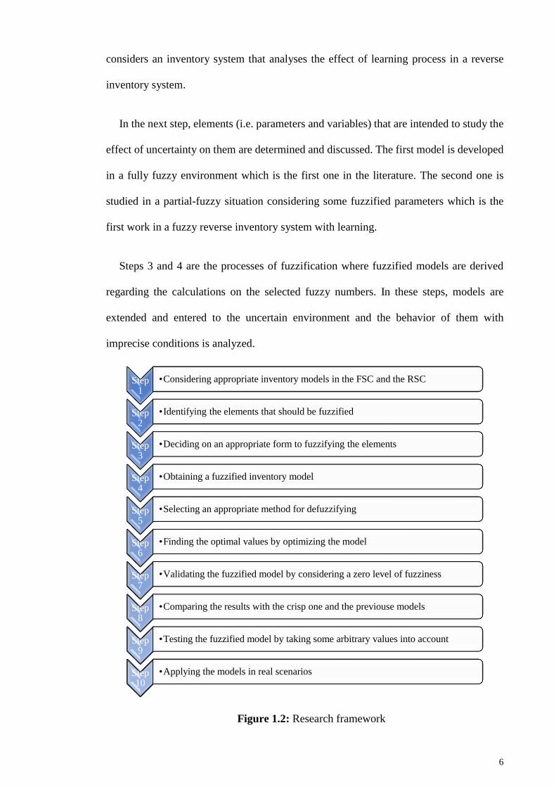
The applied methodology in Figure 1.2 has been explained. Generally, it includes 10

steps in which each step has some details.

After a comprehensive review of the related literature, two inventory models are

selected to develop in the uncertain environment. These models have some special

characteristics. The first model is a well-known inventory control model which includes

the imperfect quality items in a forward supply chain management. The second one

6

considers an inventory system that analyses the effect of learning process in a reverse

inventory system.

In the next step, elements (i.e. parameters and variables) that are intended to study the

effect of uncertainty on them are determined and discussed. The first model is developed

in a fully fuzzy environment which is the first one in the literature. The second one is

studied in a partial-fuzzy situation considering some fuzzified parameters which is the

first work in a fuzzy reverse inventory system with learning.

Steps 3 and 4 are the processes of fuzzification where fuzzified models are derived

regarding the calculations on the selected fuzzy numbers. In these steps, models are

extended and entered to the uncertain environment and the behavior of them with

imprecise conditions is analyzed.

Figure 1.2: Research framework

Step 1

•Considering appropriate inventory models in the FSC and the RSC

Step 2

•Identifying the elements that should be fuzzified

Step 3

•Deciding on an appropriate form to fuzzifying the elements

Step 4

•Obtaining a fuzzified inventory model

Step 5

•Selecting an appropriate method for defuzzifying

Step 6

•Finding the optimal values by optimizing the model

Step 7

•Validating the fuzzified model by considering a zero level of fuzziness

Step 8

•Comparing the results with the crisp one and the previouse models

Step 9

•Testing the fuzzified model by taking some arbitrary values into account

Step 10

•Applying the models in real scenarios

7

As correct policies have to be reported to the decision makers precisely, therefore, the

next step is devoted to transform the imprecise models to the certain ones with an

appropriate method. The results extracted from the process of defuzzification can be

applied in the real business environment.

Derived models from the previous steps are discuss how to be optimized in the next

stage. Regarding the literature, there are many optimization techniques to obtain the

optimal policies. However, it depends on the level of the complexity of the model which

method is appropriate and results the best solution. Optimization of the first model is

based on the Karush-Kuhn-Tucker theorem (Taha, 1997) while the second one is

optimized using a suggested algorithm.

In the next three stages, models with some arbitrary levels of fuzziness and data are

validated, compared and tested. Finally, the application of the models is shown in the real

case studies.

1.7 Thesis Layout

In this chapter, general framework of the research is overviewed. In the next chapter,

EPQ and EOQ models in the literature that are developed in fuzzy situation are

comprehensively overviewed. Chapter three is devoted to explain the methodology and

techniques that are used to develop and solve the fuzzy inventory models. In chapter 4,

the first fuzzy EOQ models are discussed and their characteristics are analyzed. The effect

of fuzziness on the second model which is a reverse inventory system is discussed in

chapter 5. To show the applicability of the developed models, they are illustrated applying

real scenarios in chapter 6. Finally, the research is concluded in the last chapter.

8

CHAPTER 2: LITERATURE REVIEW

2.1 Introduction

To place the contribution of the proposed fuzzy inventory models in the right

perspective, a systematic literature review is conducted and the previous literature

categorizing the related papers in some classifications is studied. In fact, a systematic

literature review is an approach to summarize the body of existing research on a specific

topic, which aims at analyzing the conceptual content of the field, identifying patterns

and research streams, and discovering the strengths and weaknesses of selected literature

(Hochrein & Glock, 2012). Fuzzy inventory models through two main categories are

divided: (1) economic order quantity (EOQ) models, and (2) economic production

quantity (EPQ) models. In the next step, some subcategories are considered for the

mentioned categories.

Contents of the investigated papers are analyzed in this chapter. Some tables are

provided to compare the investigated studies from the fuzzified elements and

characteristics points of view. Other tables in the next chapter are presented while the

research methodology of our study is explained technically.

2.2 Inventory Management

Inventory control and management is one of the most important fields in supply chain

management. It becomes more and more important for the enterprises in the real-life

situations. Inventory problems are common in manufacturing, remanufacturing,

maintenance service and business operations in general. Inventory is one of the costliest

operating expenses through the other activities of a supply chain for many manufacturing

industries. A proper control and analyzing of inventory systems can significantly enhance

a company’s profit (Wang et al., 2007a). In fact, the management of inventory is a vital

issue in optimizing productivity and profitability in many industries. For this reasons,

9

investigating inventory management is a critical point for many service and

manufacturing industries and many world-wide scholars are interested to find solutions

for the inventory management problems using different mathematical point of view.

In recent years, many inventory models including economic order quantity (EOQ)

model, economic production quantity (EPQ) model, joint economic lot size (JEL) model,

newsvendor model, multi-period inventory model and multi-item inventory model have

been developed. These models have been extended by applying other techniques and

methods. In the next two sections, studies concerning the EO/PQ models considering the

fuzzy set theory are reviewed.

2.3 Fuzzy Set Theory

In order to cope with the ambiguity of input parameters in the realistic environment,

the Fuzzy Set Theory (FST) introduced by Zadeh (1965) is recognized as a powerful tool

which has received considerable attentions from researchers. The FST becomes a proper

method to handle decision-making and reduces risky decision-making where there are

vague conditions or no data is available. The property which differentiates the FST from

other methods is its capability to utilize decision maker’s opinion in an inventory system

where its characteristics and data are very complicated. There are many situations in

industry where the attributes of the input parameters are complicated so that they can be

determined based on the experiences of policy makers and represented by the FST. The

application of the FST can permit flexibility in defining the vague parameters which

enables the model to handle uncertainties.

2.4 Fuzzy Inventory Management

As the parameters and variables in an inventory model may be derived and estimated

by uncertain datum, it is very hard to define a real inventory system exactly using precise

terms. Although, in this case, probability theory can be used to estimate the system, some

10

issues make it difficult to estimate the probability distribution of the elements of an

inventory system because of (1) absence of historical data, and (2) imprecise nature of

data. On one hand, estimation of parameters in the cost functions using traditional

econometric methods which use probability theory is not always possible due to

insufficient historical data specially, for newly launched products (Guchhait et al., 2014).

On the other hand, ignoring uncertainty in the inventory management usually leads to

some results that are not compatible with the real world.

Uncertainty of inventory models is a well-established phenomenon in recent years.

Extensive research works have been made on stochastic inventory models (Sox et al.,

1999; Winands et al., 2011). Since 1965 when Zadeh (1965) introduced fuzzy set theory

to cope quantitatively with uncertain information in making proper decisions, inventory

models have been extended by applying of this theory. The associated problem becomes

a fuzzy inventory model. Fuzzy set theory gives an opportunity to handle inventory

models containing imprecise linguistic terms and vagueness in real life situations. In fact,

it provides relaxation in fitting of the probability distribution function to deal with these

types of situations (Kumar & Goswami, 2015b).

The first fuzzy inventory models that appeared in the literature is believed to be that

of Sommer (1981) and Kacprzyk and Stanieski (1982) who used a fuzzy dynamic

programming approach and fuzzy set theory to solve a real world production-inventory

scheduling problem with capacity constraints, and problem of controlling inventory over

an infinite planning horizon, respectively. In the first work, linguistic statements such as

“the stock should be at best zero at the end of the planning horizon” and “diminish

production capacity as continuously as possible” were utilized to explain management’s

fuzzy aspirations for inventory and production capacity reduction in a planned withdrawal

from a market. In the second one, considering a fuzzy inventory level and fuzzy

11

replenishment as the output and input, respectively, where demand and system constraints

on replenishment are also fuzzy, an inventory system was designed. They presented an

algorithm to find the optimal time-invariant strategy for determining the replenishment to

current inventory levels that maximizes the membership function for the decision.

2.5 Methodology of Literature Review

The general framework to do the literature review of this research is based on the

method designed by Mayring (2010). Four steps are considered including gathering the

related papers, descriptive analysis, classification of the works, and content evaluation of

the gathered studies as depicted in Figure 2.1. They are explained in the following. In the

next stage, the content of the investigated studies is analyzed.

Figure 2.1: Research methodology framework (Mayring, 2010)

2.5.1 Material Collection

Journals which are indexed in Social Sciences Citation Index and Web of Science

previously known as Web of Knowledge, the “Web of Science™ tore Collection”

including Science Citation Index Expanded (SCI-EXPANDED) and Social Sciences

Citation Index (SSCI) are chosen. Keywords such as “fuzzy”, “EOQ”, “EPQ”,

“inventory”, “economic order quantity”, “economic production quantity”, and “model”

were searched through these databases separately or with each other. All papers that have

been published since 1980 are considered. It should be noted that because of the vast

number of publications in this area, our review is limited to consider only the papers

published in ISI journals (indexed in Journal Citation Reports by Thomson Reuters).

Later, to ensure the coverage of all related papers, other well-known databases including

12

Scopus, Elsevier, Springer, Taylor & Francis, Wiley, IEEE Xplore, Emerald,

Inderscience, and ABI/INFORM Complete to find relevant studies published in journals

that are indexed by Institute for Scientific Information (ISI) are searched.

2.5.2 Descriptive Analysis

The sample of 130 papers in the previous step was subject to an assessment in terms

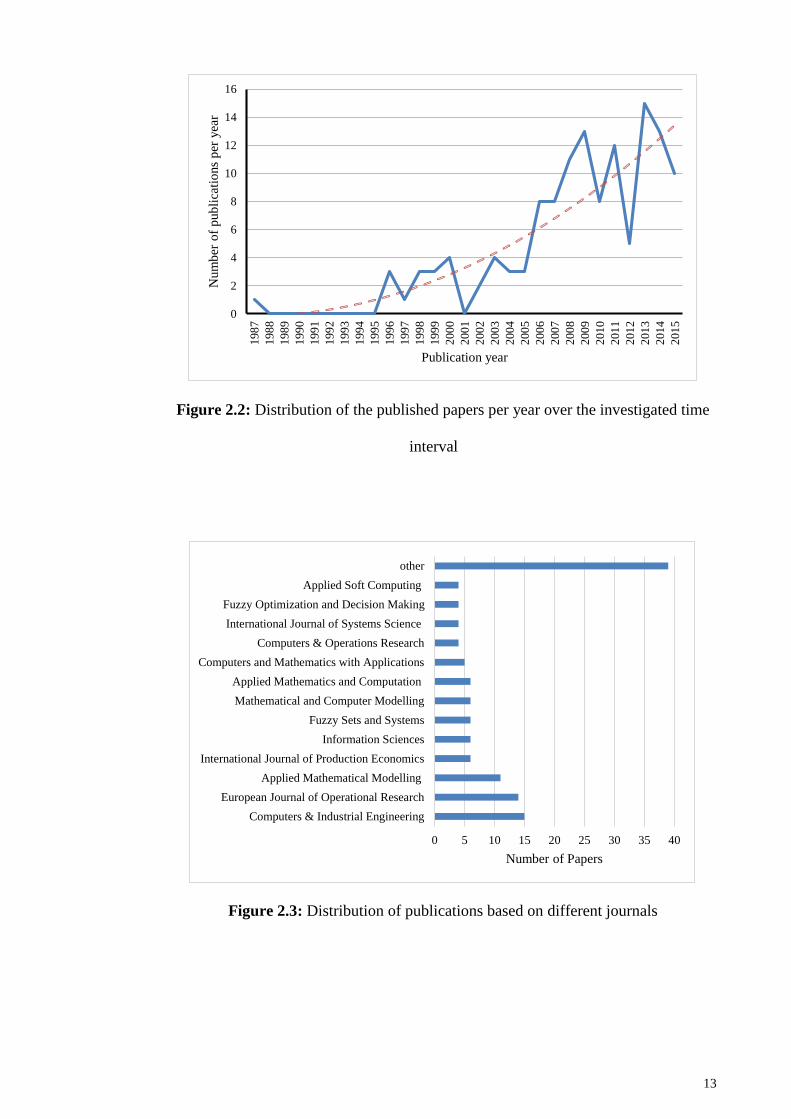
of descriptive analysis. Figure 2.2 illustrates the yearly distribution of the papers over 29

years’ time frame.

Overall, the trend line indicates that the topic of fuzzy inventory management with the

focus of fuzzy EOQ (FEOQ) and fuzzy EPQ (FEPQ) has become increasingly popular

throughout the years. The years on which the higher number of papers was published

were 2009, 2011 and 2013, with 13, 12 and 15 papers respectively. Interestingly, even

though the first paper published in 1987, this area was unnoticed for 7 years until the

second paper published in 1996. Moreover, roughly 82% of the papers published

throughout the recent 10 years, highlights the importance of this domain for researchers.

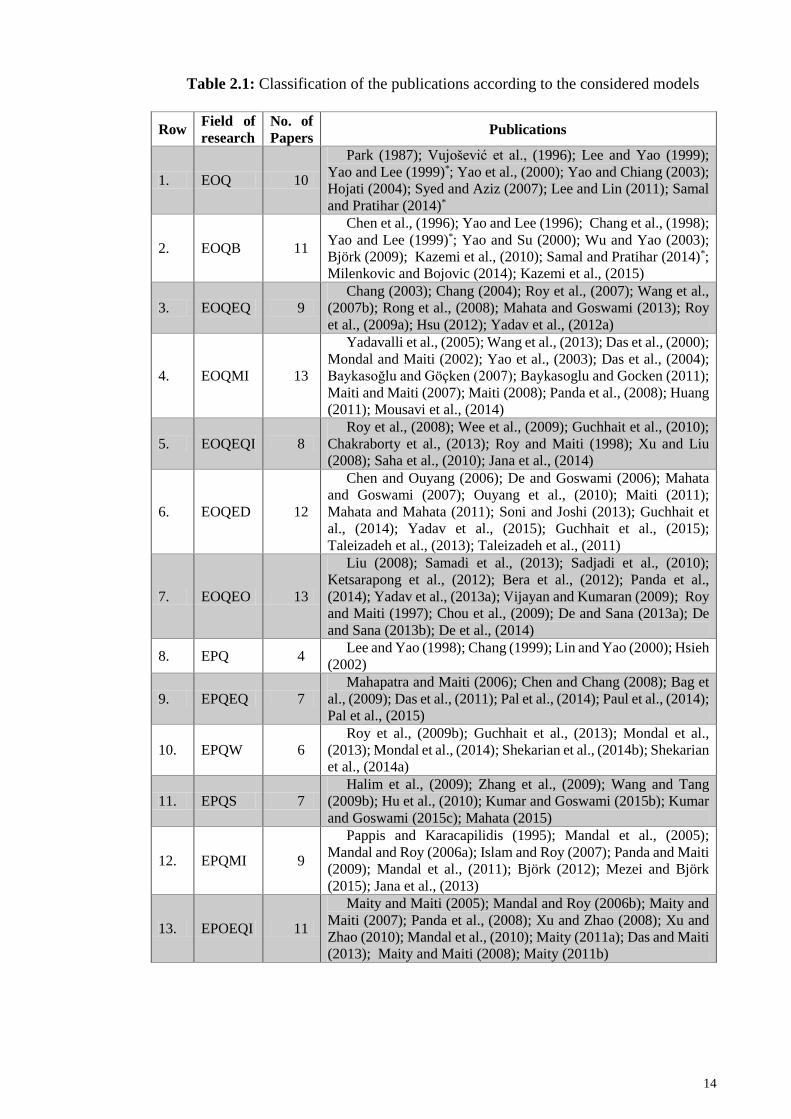
Figure 2.3 ranks the academic peer-reviewed journals as to the number of papers that

they published about this topic. Due to the variety of the journals in this realm, only the

journals with four or more publications are provided in this figure, and other journals are

grouped in a general category namely “others”. As can be seen, Computers & Industrial

Engineering (CAIE), European Journal of Operational Research (EJOR), and Applied

Mathematical Modelling (AMM) are the four primary journals published the models on

fuzzy inventory management, which account for almost 31% of the entire papers.

2.5.3 Category Selection

After finalizing the collected papers, these sample papers were categorized regarding

two main categories including EOQ and EPQ models.

13

Figure 2.2: Distribution of the published papers per year over the investigated time

interval

Figure 2.3: Distribution of publications based on different journals

0

2

4

6

8

10

12

14

16

198

7

198

8

198

9

199

0

199

1

199

2

199

3

199

4

199

5

199

6

199

7

199

8

199

9

200

0

200

1

200

2

200

3

200

4

200

5

200

6

200

7

200

8

200

9

201

0

201

1

201

2

201

3

201

4

201

5

Num

ber

of

pub

lica

tio

ns

per

yea

r

Publication year

0 5 10 15 20 25 30 35 40

Computers & Industrial Engineering

European Journal of Operational Research

Applied Mathematical Modelling

International Journal of Production Economics

Information Sciences

Fuzzy Sets and Systems

Mathematical and Computer Modelling

Applied Mathematics and Computation

Computers and Mathematics with Applications

Computers & Operations Research

International Journal of Systems Science

Fuzzy Optimization and Decision Making

Applied Soft Computing

other

Number of Papers

14

Table 2.1: Classification of the publications according to the considered models

Row Field of

research

No. of

Papers Publications

1. EOQ 10

Park (1987); Vujošević et al., (1996); Lee and Yao (1999);

Yao and Lee (1999)*; Yao et al., (2000); Yao and Chiang (2003);

Hojati (2004); Syed and Aziz (2007); Lee and Lin (2011); Samal

and Pratihar (2014)*

2. EOQB 11

Chen et al., (1996); Yao and Lee (1996); Chang et al., (1998);

Yao and Lee (1999)*; Yao and Su (2000); Wu and Yao (2003);

Björk (2009); Kazemi et al., (2010); Samal and Pratihar (2014)*;

Milenkovic and Bojovic (2014); Kazemi et al., (2015)

3. EOQEQ 9

Chang (2003); Chang (2004); Roy et al., (2007); Wang et al.,

(2007b); Rong et al., (2008); Mahata and Goswami (2013); Roy

et al., (2009a); Hsu (2012); Yadav et al., (2012a)

4. EOQMI 13

Yadavalli et al., (2005); Wang et al., (2013); Das et al., (2000);

Mondal and Maiti (2002); Yao et al., (2003); Das et al., (2004);

Baykasoğlu and Göçken (2007); Baykasoglu and Gocken (2011);

Maiti and Maiti (2007); Maiti (2008); Panda et al., (2008); Huang

(2011); Mousavi et al., (2014)

5. EOQEQI 8

Roy et al., (2008); Wee et al., (2009); Guchhait et al., (2010);

Chakraborty et al., (2013); Roy and Maiti (1998); Xu and Liu

(2008); Saha et al., (2010); Jana et al., (2014)

6. EOQED 12

Chen and Ouyang (2006); De and Goswami (2006); Mahata

and Goswami (2007); Ouyang et al., (2010); Maiti (2011);

Mahata and Mahata (2011); Soni and Joshi (2013); Guchhait et

al., (2014); Yadav et al., (2015); Guchhait et al., (2015);

Taleizadeh et al., (2013); Taleizadeh et al., (2011)

7. EOQEO 13

Liu (2008); Samadi et al., (2013); Sadjadi et al., (2010);

Ketsarapong et al., (2012); Bera et al., (2012); Panda et al.,

(2014); Yadav et al., (2013a); Vijayan and Kumaran (2009); Roy

and Maiti (1997); Chou et al., (2009); De and Sana (2013a); De

and Sana (2013b); De et al., (2014)

8. EPQ 4 Lee and Yao (1998); Chang (1999); Lin and Yao (2000); Hsieh

(2002)

9. EPQEQ 7

Mahapatra and Maiti (2006); Chen and Chang (2008); Bag et

al., (2009); Das et al., (2011); Pal et al., (2014); Paul et al., (2014);

Pal et al., (2015)

10. EPQW 6

Roy et al., (2009b); Guchhait et al., (2013); Mondal et al.,

(2013); Mondal et al., (2014); Shekarian et al., (2014b); Shekarian

et al., (2014a)

11. EPQS 7

Halim et al., (2009); Zhang et al., (2009); Wang and Tang

(2009b); Hu et al., (2010); Kumar and Goswami (2015b); Kumar

and Goswami (2015c); Mahata (2015)

12. EPQMI 9

Pappis and Karacapilidis (1995); Mandal et al., (2005);

Mandal and Roy (2006a); Islam and Roy (2007); Panda and Maiti

(2009); Mandal et al., (2011); Björk (2012); Mezei and Björk

(2015); Jana et al., (2013)

13. EPOEQI 11

Maity and Maiti (2005); Mandal and Roy (2006b); Maity and

Maiti (2007); Panda et al., (2008); Xu and Zhao (2008); Xu and

Zhao (2010); Mandal et al., (2010); Maity (2011a); Das and Maiti

(2013); Maity and Maiti (2008); Maity (2011b)

15

Table 2.1: Continue.

Row Field of

research

No. of

Papers Publications

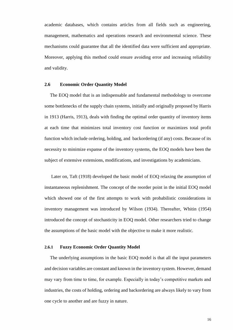
14. EPQEO 12

Islam and Roy (2006); Mahapatra et al., (2011); Chang and

Chang (2006); Chang et al., (2006); Maity et al., (2008); Pal et al.,

(2009); Wang and Tang (2009a); Soni and Shah (2011);

Chakrabortty et al., (2013); Yaghin et al., (2013); De and Sana

(2014); Kumar and Goswami (2015a)

* This paper includes two kinds of models.

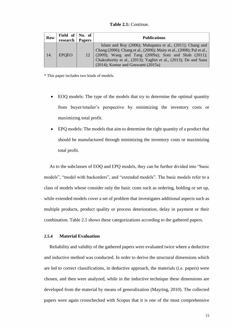
EOQ models: The type of the models that try to determine the optimal quantity

from buyer/retailer’s perspective by minimizing the inventory costs or

maximizing total profit.

EPQ models: The models that aim to determine the right quantity of a product that

should be manufactured through minimizing the inventory costs or maximizing

total profit.

As to the subclasses of EOQ and EPQ models, they can be further divided into “basic

models”, “model with backorders”, and “extended models”. The basic models refer to a

class of models whose consider only the basic costs such as ordering, holding or set up,

while extended models cover a set of problem that investigates additional aspects such as

multiple products, product quality or process deterioration, delay in payment or their

combination. Table 2.1 shows these categorizations according to the gathered papers.

2.5.4 Material Evaluation

Reliability and validity of the gathered papers were evaluated twice where a deductive

and inductive method was conducted. In order to derive the structural dimensions which

are led to correct classifications, in deductive approach, the materials (i.e. papers) were

chosen, and then were analyzed, while in the inductive technique these dimensions are

developed from the material by means of generalization (Mayring, 2010). The collected

papers were again crosschecked with Scopus that it is one of the most comprehensive

16

academic databases, which contains articles from all fields such as engineering,

management, mathematics and operations research and environmental science. These

mechanisms could guarantee that all the identified data were sufficient and appropriate.

Moreover, applying this method could ensure avoiding error and increasing reliability

and validity.

2.6 Economic Order Quantity Model

The EOQ model that is an indispensable and fundamental methodology to overcome

some bottlenecks of the supply chain systems, initially and originally proposed by Harris

in 1913 (Harris, 1913), deals with finding the optimal order quantity of inventory items

at each time that minimizes total inventory cost function or maximizes total profit

function which include ordering, holding, and backordering (if any) costs. Because of its

necessity to minimize expanse of the inventory systems, the EOQ models have been the

subject of extensive extensions, modifications, and investigations by academicians.

Later on, Taft (1918) developed the basic model of EOQ relaxing the assumption of

instantaneous replenishment. The concept of the reorder point in the initial EOQ model

which showed one of the first attempts to work with probabilistic considerations in

inventory management was introduced by Wilson (1934). Thereafter, Whitin (1954)

introduced the concept of stochasticity in EOQ model. Other researchers tried to change

the assumptions of the basic model with the objective to make it more realistic.

2.6.1 Fuzzy Economic Order Quantity Model

The underlying assumptions in the basic EOQ model is that all the input parameters

and decision variables are constant and known in the inventory system. However, demand

may vary from time to time, for example. Especially in today’s competitive markets and

industries, the costs of holding, ordering and backordering are always likely to vary from

one cycle to another and are fuzzy in nature.

17

Therefore, there is a need to develop fuzzy EOQ models to capture the uncertainties

accurately. A number of fuzzy inventory models have already been proposed and studied

in the literature. The first FEOQ model proposed by Park (1987) who examined an EOQ

model by treating ordering and holding costs as trapezoidal fuzzy numbers, used the

extension principle for defuzzifying and solved the model with numerical operations.

Earlier, many researchers developed other FEOQ models.

2.6.1.1 Fuzzy Economic Order Quantity Model without Backorder (EOQ)

To determine the effect of different approaches to obtain the optimal order quantity,

Vujošević et al., (1996) solved an EOQ model with ordering and holding costs and four

different solution procedures based on the ranking of fuzzy number and the center of

gravity method in a fuzzy environment. It was shown that they give different solutions at

which the fuzzy cost function attains its minimum, simply because they handle

uncertainty in different ways. There are some problems and shortcomings in this study

which were discussed and highlighted by Hojati (2004) and could be improved. He argued

that the suggested solution procedures are complicated and time consuming, for example.

Yao and Lee (1999) and Lee and Yao (1999) fuzzified order quantity to trapezoidal

and triangular fuzzy number in the total cost of inventory model without backorder,

respectively. In both studies, the results showed that after defuzzification the total cost is

slightly higher than in the crisp model. In a follow-up study, Yao et al., (2000)

investigated an EOQ problem without backorder such that both the order and the total

demand quantities are triangular fuzzy numbers. They used a computer program to find

the total cost in the fuzzy sense. In order to compare the results of different defuzzification

methods (i.e. the centroid and the signed distance) in the total cost of inventory model

without backorders, where the total demand and the cost of storing one unit per day is

18

supposed to be triangular fuzzy numbers, another study was conducted (Yao & Chiang,

2003). They proposed some policies to choose the appropriate defuzzification method.

In contrast to previous studies, Wang et al., (2007a) characterized the order and the

holding costs as fuzzy variables, and constructed two models using the concepts of

possibility/necessity and credibility measures: (1) a fuzzy expected value (FEV) model,

and (2) a fuzzy dependent chance programming (FDCP) model while in order to solve

these complex models, a particle swarm optimization (PSO) algorithm based on the fuzzy

simulation was designed. Syed and Aziz (2007) and Lee and Lin (2011) investigated a

fuzzy inventory model with the signed distance method. Similar to the presented approach

by Wang et al., (2007a), two variable demand inventory models, with and without

backorder, building FEV and FDCP models, were constructed for minimizing inventory

cost, treating the holding, ordering and backordering costs and demand as independent

fuzzy variables (Samal & Pratihar, 2014). Using genetic and PSO algorithms, they

minimized the FEV of the total cost, so that the credibility of the total cost not exceeding

a certain budget level was maximized. Comparison of these algorithms proofed when the

complexity of the model is increased, PSO has outperform the GA because its particles

maintain their memory.

2.6.1.2 Fuzzy Economic Order Quantity Model with Backorder (EOQB)

One of the first attempt to build a FEOQ model with backorder is that of Chen et al.,

(1996) who considered an inventory model where yearly demand and inventory costs

including order, holding, and backorder costs were fuzzified. They used the function

principle and the median rule to find the optimal order quantity and the shortage quantity.

Yao and Lee (1996) and Chang et al., (1998) fuzzified the order and the shortage

quantity, respectively, as the normal triangular fuzzy number in an EOQ model with

backorder. They used two similar approaches to discuss fuzzy sets concepts in the

19

mentioned model. Besides, Yao and Su (2000) used interval-valued fuzzy set to consider

the total demand quantity in inventory with backorder for whole of the plan period. To

determine the effects of fuzzification of the order and shortage quantities simultaneously

in an EOQ model with backorder, Wu and Yao (2003) showed that fuzzification of both

of them could give better results than fuzzifying any one variable separately.

Björk (2009) presented the analytical solution to study the effect of uncertainty on

backorders and the lead times as well as the demand. In this case, according to a numerical

example, the orders were approximately 6% higher than for the crisp case. In addition,

comparing the obtained results with those of Chang et al., (1998) showed that they are

coherent. In this line of research, a fully fuzzy EOQ model with backorder, where all the

input parameters and the decision variables are simultaneously fuzzified in two different

cases with both trapezoidal and triangular fuzzy numbers, was conducted by Kazemi et

al., (2010). Their results, which were more sensitive to changes in the input parameters

when triangular fuzzy numbers were used, contribute that the changes in the values of the

decision variables (the maximum inventory level and the batch size) to changes in the

costs between the crisp (deterministic) and fuzzy cases have a linear relationship. Similar

to the approach used by Björk (2009), a fuzzy EOQ model to the sizing of empty cars on

a rail network tested with a real case of the Serbian rail network within a four-day

planning period to derive freight car inventory level in station i for period n of the

planning horizon and the ordering quantity for the same station and period n as decision

variables was proposed (Milenkovic & Bojovic, 2014). They assumed lead time as the

time of the freight car traveling between two stations. The work of Björk (2009) was

extended by Kazemi et al., (2015) who relaxed the assumption of constant fuzziness by

incorporating the concept of learning in fuzziness into the model. They showed that the

total cost of the fuzzy inventory model under learning is less than the fuzzy case without

learning.

20

2.6.1.3 Extensions of Fuzzy Economic Order Quantity Model

In this section, the content of the gathered EOQ papers based on the categorizations

which are based on the quality of items, the number of items, delay in payment and other

extensions are explained.

Quality Based Studies (EOQEQ)

Chang (2003) reformulated the model developed by Porteus (1986) drawing on the

concept of imperfect production process with opportunity cost rate as a statistic-fuzzy

number. He derived the optimal values of lot size and the process quality level in the

fuzzy sense utilizing the logarithmic investment cost function. Building upon the work of

Salameh and Jaber (2000) who constructed an EOQ model with imperfect quality, Chang

(2004) incorporated the fuzziness of defective rate and the annual demand into the

mentioned EOQ model. He employed the signed distance method to find the estimate of

total profit per unit time in the fuzzy sense, and then derived the corresponding optimal

lot size. Roy et al., (2007) considered a two storage inventory model under bulk release

pattern between two warehouses in a stochastic planning horizon with an exponential

distribution where demand and deterioration are stock dependent and fuzzy, respectively.

Considering the imperfect quality items in each delivered lot, Wang et al., (2007b)

developed an EOQ model with the percentage of imperfect quality items in each lot as a

random fuzzy variable. They assumed the inspection, the holding, and the setup costs as

fuzzy variables and maximized expected long-run average profit by constructing a

random fuzzy expected value model which was solved by a PSO algorithm based on the

random fuzzy simulation. Rong et al., (2008) introduced a two-warehouse problem for

deteriorating items with fuzzy lead time where ordering cost assumed to be partly lead

time dependent. Roy et al., (2009a) formulated a fuzzy inventory model of a deteriorating

item with displayed stock dependent demand over a stochastic time horizon. Considering

the learning effects on percentage of defective items, Yadav et al., (2012a) formulated a

21

FEOQ model with backorder by taking fuzzified demand rate with dependence upon the

frequency of advertisement, while in contrast to previous usual methods, optimal values

were obtained by using algebraic method instead of differential calculus. According to

some analytically and numerically results, they proved that the number of defective units

and shipment size decrease, whereas backordering level and net profit increase as learning

increases and as it becomes faster. Therefore, it was recommended to order in smaller lots

less frequently. Hsu (2012) explored a fuzzy inventory model with immediate return for

defective items. By extending the work of Wee et al., (2007) who focused on the quality

of items and full backordering, Mahata and Goswami (2013) developed two fuzzy

inventory models in which in the first model the maximum backordering quantity and the

order size as decision variables are fuzzified, and in the second one, not only decision

variables but also all the parameters are fuzzified. They concluded that the optimal

solutions of the second model are same as those under the fuzzy model with the crisp

decision variables, and moreover, the decision variables and the annual total profit are

highly sensitive due to the fuzziness in the input parameters. It is such that the percentage

change due to fuzziness causes approximately double percentage changes in the annual

total profit and the backordering quantity is nearly equal of the changes in the

components, whereas the order lot size changes marginally.

Multi-Item Models (EOQMI)

A model similar to Roy and Maiti (1998)’s approach where inventory costs were

directly proportional to the respective quantities, and unit purchase/production cost was

inversely related to the demand was investigated (Das et al., 2000). Besides, fuzzy non-

linear programming problem (FNLP) along with genetic algorithm (GA), for the first

time, were applied to solve multi-item FEOQ models under fuzzy objective of cost

minimization and imprecise constraints on warehouse space and number of production

runs with crisp/imprecise inventory costs (Mondal & Maiti, 2002). For two mutually

22

complementary merchandises, Yao et al., (2003) discussed how to determine the optimal

ordering policy with fuzzy concept. Applying a new solving approach, Das et al., (2004)

formulated a multi-item fuzzy-stochastic inventory model under total budgetary and

space constraints. They reduced the model to a corresponding equivalent fuzzy non-linear

programming problem, and then, it is solved by FNLP following Zimmermann (1975)

technique. Following the work of Roy and Maiti (1995), FEOQ models were developed

for multiple items (Yadavalli et al., 2005). The authors showed that among various

membership functions, linear membership function provides the best values with the

maximum aspiration level. Baykasoğlu and Göçken (2007) solved a fuzzy multi-item

EOQ problem with fuzzification of all the parameters as triangular fuzzy numbers except

the demand per unit time for the ith item which was assumed crisp by employing four

different fuzzy ranking methods which are the signed distance, integral value, possibility

programming, and expected intervals method. The results showed that models based on

different ranking procedures generated different solutions to the problem and,

furthermore, the solution of the model based on the integral value ranking approach

generated better results than the other ones. In a similar study, Baykasoglu and Gocken

(2011) compared the results of the considered model of their previous research

(Baykasoğlu & Göçken, 2007) with those of obtained by PSO algorithm as a direct

approach. It was concluded by applying a transformation process (i.e. indirect approach)

some of the information can be missed; and it highlights the importance of the proper

selection of a fuzzy ranking procedure in the direct method. They showed that fuzzy

optimization problems can be easily solved using fuzzy ranking and metaheuristics

methods without any necessity of transformation into a crisp equivalent.

Fuzzy-stochastic multi-item inventory models with two storage facility and bulk

release were solved using a possibility/necessity based optimization technique (Maiti &

Maiti, 2007). Maiti (2008) developed a fuzzy two-storage inventory model incorporating

23

simultaneous ordering and transferring, following basic period (BP) approach. Panda et

al., (2008a) formulated an inventory model with hybrid inventory costs and fuzzy/fuzzy-

stochastic resources where unit cost is demand dependent. Huang (2011) compared the

performance of two well-known defuzzification methods (i.e. signed distance and

centroid methods) proposing a multi-level lot-sizing problem for multi-item. In an inter-

disciplinary research of a fuzzy inventory model and intelligent optimization algorithms,

Wang et al., (2013) formulated a FDCP inventory model in a joint replenishment problem

(JRP). Mousavi et al., (2014) solved a fuzzy multi-product/period inventory problem

using intelligence algorithms under an incremental quantity. According to their results,

the performance of the harmony search algorithm to optimize the single and bi-objective

inventory control is better than the PSO one.

Mix Quality Multi-Item Studies (EOQEQI)

Roy and Maiti (1998) formulated two fuzzy multi-item multi-objective inventory

models with stock dependent demand which were solved by FNLP and fuzzy additive

goal programming (FAGP) methods. Later, these models were extended in a fuzzy

random environments by Xu and Liu (2008) where a method of solving solution sets of

fuzzy random multi-objective programming problems was designed and applied to

numerical inventory problems with all inventory costs, purchasing and selling prices in

the objectives and constraints assumed as fuzzy random variables in nature. They

extended a method to find the membership function of the fuzzy total inventory while the

related fuzzy inventory problem is solved via two techniques: (1) fuzzy extension

principle and duality, and (2) nearest interval approximations for fuzzy numbers.

Using a similar approach to Liu (2008), a deteriorating multi-item inventory system

subject to constraints on fuzzy costs and storage space was proposed (Roy et al., 2008).

Wee et al., (2009) developed a fuzzy multi-objective joint replenishment deteriorating

24

items inventory model with fuzzy demand and shortage cost constraint, and maximized

the profit and return on inventory investment objectives simultaneously. Regarding the

breakable items which get damaged because of the accumulated stress of heaped stocks

during storage, Saha et al., (2010) formulated fuzzy multi-item inventory models with

stock dependent demand supposing that the number of damaged items depends only on

the current stock level linearly and non-linearly. They assumed more options: (1) the

demand depends on the current stock but becomes constant when the stock falls below a

certain level, and (2) the breakability of the items is up to a certain stock level and

thereafter, there is no breaking of the items when the stock falls below the level. In

addition, Guchhait et al., (2010) proposed fuzzy inventory models of breakable items,

where demand of the items are stock dependent and breakability rates increase linearly

with stock and nonlinearly with time. Chakraborty et al., (2013) addressed an inventory

model of deteriorating seasonal products for a wholesaler having showrooms at different

places under a random planning horizon with different discounting policies. Besides, Jana

et al., (2014) formulated a multi-item fuzzy inventory models under random planning

horizon and stock-dependent demand.

Studies with Delay in Payment (EOQED)

With a permissible delay in payment, De and Goswami (2006) extended an EOQ

model with a fuzzy inflation rate and fuzzy deterioration rate. They discussed three cases

where shortage time is smaller, equal or greater than the permissible delay period for

settling accounts and the duration of the permissible delay time effectively changes the

optimal system cost. These situations were compared with the help of numerical

examples. Chen and Ouyang (2006) extended the work of Jamal et al., (1997) considering

the rate of the carrying cost, interest paid/earned simultaneously fuzzified based on the

interval-valued fuzzy number and triangular fuzzy number. They indicated that there

exists a unique interior optimal solution to the proposed model. Another work in this area

25

regarding deteriorating items, is that of Mahata and Goswami (2007) who extended the

delay in payments not only for the retailer but also for the customer. Furthermore, the

graded mean integration representation (GMIR) method was used for defuzzifying the

total variable cost which was derived from fuzzified variables comprising the demand

rate, and the holding, ordering, and purchasing costs.

Allowing delay in payments, Ouyang et al., (2010) fuzzified the work of Chang et al.,

(2003) who linked the supplier credits to ordering quantity. Maiti (2011) introduced

customers’ credit-period linked dynamic demand with the imprecise planning horizon

due to the competitive market.

Under the assumption of having the full trade credit offered by suppliers for the retailer

due to their powerful position and just offering a partial trade credit to customers by

retailer, Mahata and Mahata (2011) investigated a FEOQ model in a two levels of trade

credit. They derived optimal values and proposed some policies. Besides, they obtained

some previously published results of other authors as special cases. Their work was

extended by Soni and Joshi (2013) adding more realistic assumptions such as imprecise

selling price dependent demand rate.

Regarding a variable demand which depends on selling price, stock level and retailer’s

credit period, Guchhait et al., (2014) developed a FEOQ model of a deteriorating item

where not only supplier to the retailer but also retailer to his customer could provide

permissible delay in payment and the supplier could consider cash discount to the retailer

to pay for their purchases quickly. Yadav et al., (2015) considering the trade credit policy

in a fuzzy environment concluded that the retailer can increase the profit by ordering

lower quantity. Guchhait et al., (2015) presented an inventory policy for the time-

dependent deteriorated goods with different types of imprecise inventory costs, two-level

partial trade credit facility and credit period dependent demand. Taleizadeh et al., (2011)

26

and Taleizadeh et al., (2013) extended fuzzy rough joint replenishment multi-product

multi-constraint inventory models as mixed integer nonlinear programming to purchase

high price raw materials that are solved by meta heuristic algorithms.

Other Extensions of EOQ (EOQEO)

Roy and Maiti (1997) formulated a FEOQ model with limited storage capacity where

the demand is related to the unit price and the setup cost varies with the quantity

produced/purchased and the fuzziness is introduced in both objective function and storage

area. They applied FNLP to solve their model. Later, their analytical procedure was

improved by employing formulated solutions based on the max–min operator (Chou et

al., 2009). Pointing out the questionable results and resolving the deficiencies to obtain

the minimum solution of previous work by Roy and Maiti (1997), with the same inventory

model with fuzzy constraints, Chou et al., (2009) proposed a method based on the max–

min operator and solved the deterministic inventory model converted from the fuzzy

inventory model. Liu (2008) revisited an EOQ model as a profit maximization problem

when the demand quantity and the unit cost are fuzzy numbers, and are functions of the

price and lot size, respectively. He developed a solution method based on the extension

principle where the fuzzy inventory problem is transformed into a pair of two-level

mathematical programs to derive the upper bound and lower bound of the fuzzy profit at

possibility level α. Then, it is transformed into a pair of conventional geometric programs

to solve. The results showed that when the selling price is elastic, the larger the selling

price, the smaller the order quantity is. Chen (2003)’s model called economic order time

(EOT) was fuzzified when the time period of sales is the decision variable and the

components of the model are fuzzified (Vijayan & Kumaran, 2009). It was shown that

the solutions of the EOT model with all fuzzy components were the same as those under

the fuzzy model with the crisp time period.

27

Sadjadi et al., (2010) developed a new pricing and marketing planning proposing

solutions expressed by membership functions. They assumed the demand is a function of

price and marketing expenditure with fuzzy parameters, and the purchasing cost is as a

function of the order quantity. Bera et al., (2012) developed an inventory model with an

infinite rate of replenishment over a finite but imprecise time horizon considering time

dependent ramp type demand. Ketsarapong et al., (2012) developed an uncapacitated

single item lot sizing problem in a fuzzy environment that is converted to a crisp model

with the help of possibility approach.

Samadi et al., (2013) developed a FEOQ model proposing solutions expressed by

membership functions where the demand is a power function of price, marketing and

service expenditures and the unit cost is determined as a function of the order quantity.

Yadav et al., (2013a) developed a fuzzy version of the model of Lin (2008) who

considered a controllable backorder price discount and the reduction of lead-time. De and

Sana (2013a) developed an intuitionistic FEOQ where the demand rate is varying with

the selling price and the promotional effort (PE). De and Sana (2013b) dealt with a

backorder EOQ model while a 𝑚-th power promotional index (PI) as a fuzzy decision

variable was added to the total profit function along with the order and shortage quantities.

They assumed the demand as a function of the PI, and concluded that the value of PI near

zero may not give the maximum profit. Following their previous works, with PE

dependent demand allowing shortages and assuming the decrease in the demand rate in

stock out situation while it comes back to its initial rate since PE continues, they proposed

a solution procedure for an intuitionistic fuzzy (IF) backorder inventory model and made

a comparative study on Pareto optimality and optimality under Lagrange’s interpolating

polynomial function (De et al., 2014). They concluded that in contrast to the Pareto

optimality test which is valid only for minimization problem, their modified IF

programming techniques (IFPT) called interpolation method is valid for any kind of

28

(max/min) problem. Regarding the warehouse inventory systems, Panda et al., (2014)

developed a two-warehouse fuzzy-stochastic mixture problem.

2.7 Economic Production Quantity Model

Since the development of EOQ model by Harris (1913), up to now, numerous

inventory models have been studied in the literature in order to consider various realistic

features. On the other hand, economic production quantity (EPQ) model, which is an

extension of the EOQ model, has also been served for over 80 years to determine the

optimal lot size in production/inventory systems.

Needless to say that, similar to EOQ model, the results of EPQ models depend largely

on a number of basic assumptions such as types of demand, production rates, different

cost parameters, replenishment policies and so on (Halim et al., 2009). In the next section,

Studies which consider fuzzy set theory into the EPQ model to build a FEPQ model are

reviewed.

2.7.1 Fuzzy Economic Production Quantity Model

Similar to its counterpart (i.e. EOQ), economic production quantity model has been

developed through the fuzzy set theory. In recent years, many kinds of fuzzy EPQ model

were extended. In discussions of production quantity models, it is believed that Sommer

(1981) applied a fuzzy dynamic programming approach to solve a production-inventory

scheduling problem with capacity constraints. Another earlier work is that of Kacprzyk

and Stanieski (1982) who incorporated the fuzzy set theory into production planning and

control problems.

2.7.1.1 Fuzzy Basic Economic Production Quantity Model (EPQ)

By fuzzification of both the demand quantity and the production quantity per day, Lee

and Yao (1998) investigated a computing schema for the FEPQ deriving the membership

29

function of the fuzzy total cost. The triangular form, extension principle and centroid

method were used for fuzzy numbers, calculation and defuzzification, respectively. They

found that, after defuzzification, the total cost was slightly higher than in the crisp model.

Later, using the procedure used in Lee and Yao (1998), two studies were conducted by

Chang (1999) and Lin and Yao (2000) who only fuzzified the production quantity in their

model as triangular and trapezoidal fuzzy number, respectively.

Hsieh (2002) constructed two FEPQ models while the first one was fully fuzzified on

all the parameters, and in the second one, not only all parameters but also the decision

variable (i.e. production quantity) was fuzzified as a trapezoidal fuzzy number. He

showed that considered models are executable and useful in the real world.

2.7.1.2 Extensions of Fuzzy Economic Production Quantity Model

In this section, the content of the EPQ papers according to the categorizations which

are based on the quality of items, rework, the number of items, and other extensions are

explained.

Quality Based Studies (EPQEQ)

Mahapatra and Maiti (2006) addressed a production-inventory model with imprecise

preparation time for production aiming to maximize the profit. Chen and Chang (2008)

introduced a FEPQ model with defective productions that cannot be repaired. Bag et al.,

(2009) introduced the fuzzy random variable demand concept to an imperfect production

system considering reliability of production system. A production system producing

defective items due to the machine failure was addressed by Das et al., (2011). Based on

a numerical analysis, they illustrated that there is a direct relation between the production

rate and the mean duration of a breakdown. However, an inverse relation was found

between the cost of production idle-time and the production rate. Pal et al., (2014)

investigated the ramp up demand in an EPQ model with fuzzy setting. They assumed that

30

the demand is a function of time and items in stock could be deteriorated following a

Weibull distribution. They showed that the fuzzy model returns a lower total cost value

than crisp model for some values of degree of optimism and total replenishment cycles.

According to their results, the shorter the production cycle is, the lower the total cost will

be. Moreover, Paul et al., (2014) addressed a FEOQ model with fuzzy holding cost and

demand in an imperfect production system while reliability of the system was a decision

variable. They concluded that their model is more realistic and applicable than traditional

production inventory models. Pal et al., (2015) formulated a model with the ramp type

demand and the deterioration of the product. They showed the total cost in the fuzzy and

the crisp case could be equal when the decision maker is semi optimistic.

Rework Based Studies (EPQW)

Roy et al., (2009b) developed an imperfect production system where a portion of the

imperfect items could be remanufactured to as-good-as perfect quality to satisfy customer

demand, while the remaining items are irreparable, and consequently are disposed. It was

illustrated that the relation between the total profit and the fuzzy confidence level of

defective rate are opposite. Guchhait et al., (2013) addressed a FEPQ model with

remanufacturing of imperfect quality items using fuzzy differential equation and fuzzy

Riemann-integration. Following this line of thought, Mondal et al., (2013) developed a

FEPQ model in a rough environment in which the imperfect quality items could be

repaired becoming as perfect quality item. They determined that the existence of either

uncertainty or inflation has a negative impact on the total profit, and also suggested

repairing process should start up from the second cycle when repairing rate is a dynamic

control variable. Mondal et al., (2014) formulated a FEPQ problem where units are bulkly

transformed from production center to a showroom, and the rework process of defective

items starts after the production cycle. Shekarian et al., (2014b) extended a FEOQ model,

and showed that formulating the fuzzy model with a trapezoidal membership function

31

leads to a higher total cost comparing to the triangular one. It is due to the fact that

trapezoidal fuzzy number increases the dimensions of the system. Shekarian et al.,

(2014a) extended the model of Shekarian et al., (2014b) without backorder and different

fuzzy settings. They illustrated that using the signed distance method leads to a larger lot

size in comparison with the GMIR method.

Shifting in the Production Status (EPQS)

Applying a probability function with fuzzy parameters, Halim et al., (2009) examined

two different scenarios in a production system that produces imperfect items due to the

shifting to out of control state. The authors proposed that although it is difficult to

recognize which model (fuzzy and crisp) performs better, it is more appropriate to use the

fuzzy model when the fraction of defective items fluctuates. Zhang et al., (2009)

formulated a production problem which starts with in control state producing good quality

items, and then may change to out of control state during production cycle producing a

fixed fraction of defective items. They used fuzzy and random-fuzzy concepts to build

their model. In a similar situation, Wang and Tang (2009b) addressed a model with a

difference that the time until the production shifts to out of control state is a fuzzy variable

instead of being a fuzzy random variable. In contrary to Zhang et al., (2009) and Wang

and Tang (2009b), a simpler model was considered by Hu et al., (2010), who assumed

setup and holding costs as crisp parameters.

Other works that studied the effect of randomness and fuzziness include Kumar and

Goswami (2015b), Kumar and Goswami (2015c) and Mahata (2015), who represented

the time in which the system shifts from in control to out of control state as a fuzzy random

variable.

32

Multi-Item Studies (EPQMI)

One of the earliest models dealing with multi-item FEPQ models is that of Pappis and

Karacapilidis (1995), who investigated the problem of determining optimal production

runs in a batch production system. A fuzzy multi-product multi-objective EPQ system

was addressed by Mandal et al., (2005) considering the shortage and the constraints on

storage area, production cost and number of orders. Mandal and Roy (2006a) optimized

a multi-item inventory model with demand dependent inventory level and shelf-space

constraint under three different fuzzy numbers.

Islam and Roy (2007) extended a multi-item version of Islam and Roy (2006)’s model

considering different solution procedure. A similar but more complex problem as in Islam

and Roy (2007) was studied by Panda and Maiti (2009), where unit production cost was

considered to be dependent on stock level as well as demand which was given dependent

on unit selling price. A fuzzy production inventory model which the time interval between

the decision to produce and the real time of production is variable was studied in Mandal

et al., (2011). As the production with preparation time is more costly, they stressed that

the decision for production should be made as earlier as possible to reduce the production

cost. Björk (2012) investigated a fuzzy multi-item EPQ model with a finite production

rate under uncertain cycle time. He recommended cycle time with more flexible interval

for such a production system. This work was extended by Mezei and Björk (2015) to

account for backorders. Jana et al., (2013) offered FEPQ models assuming the demand

and the unit production cost as functions of stock level and the production rate

respectively. The authors found that there are not much differences between the result of

the model solving with triangular and parabolic fuzzy numbers, and the generalized

reduced gradient (GRG) approach gives lower profit than the necessity approach.

33

Mix Quality Multi-Item Studies (EPQEQI)

One of the first studies considering the deteriorated items with multi-item in a fuzzy

production-inventory system is that of Maity and Maiti (2005), who suggested a model

with demand and production rate, assumed as a function of time, in which was solved

using weighted sum method and simple differential calculus operations. Mandal and Roy

(2006b) used hybrid numbers (i.e. numbers that simultaneously contain fuzziness and

randomness properties) to present a model with imperfect quality under uncertainty. The

author found that when the weight of the objective function increases the value of

objective function decreases as a result. Maity and Maiti (2007) suggested fuzzy dynamic

production-inventory models when the demand, the production rate and the shortage level

are time dependent. A fuzzy multi-item production-inventory system was addressed by

Maity and Maiti (2008) with time dependent demand where demand could be decreased

or increased under the influence of sale degradation and advertising policy, respectively.

Panda et al., (2008b) studied the case of imperfect production process where the constraint

is stochastic or fuzzy and concluded that modeling budget and shortage constraints using

possibility measure gives the greatest total profit among all possible combinations. Xu

and Zhao (2008) formulated a multi-objective fuzzy rough production-inventory model

with imperfect quality in which the rate of production is assumed to be the same as the

rate of rework. Xu and Zhao (2010) applied the fuzzy rough set theory in a multi-objective

programming problem in a manufacturing company in China. Mandal et al., (2010)

analyzed an imperfect production system with fuzzy time period under quadratic, linear

and constant production rate. They recommended using constant production because of

the lower total production cost. The first research in fuzzy EPQ inventory which applied

fuzzy inequality as well as fuzzy objective function in modelling the production inventory

was the study of Maity (2011a), who addressed a fuzzy EPQ model in a system including

a single machine and multiple products. Firstly, Maity (2011a) investigated a FEPQ

34

model applying fuzzy inequality as well as fuzzy objective function with a single machine

and multiple products. A multi-item production inventory model with two-warehouse and

uncertain constraints was developed by Maity (2011b), who assumed that inventory level,

production and demand rates are function of time. Das and Maiti (2013) formulated a

FEPQ model with a fuzzy-stochastic constraint on storage space and an optimistic fuzzy

equality for budget.

Other Extensions of EPQ (EPQEO)

By introducing fuzziness in objective and constraint goals, a FEPQ model considering

investment for reducing setup cost and quality improvement process was proposed by

Islam and Roy (2006). Mahapatra et al., (2011) discussed a simpler version of Islam and

Roy (2006)’s model but without storage space. Taking a variety of costs into

consideration in EPQ inventory systems, Chang and Chang (2006) analyzed a problem

by accounting for the relative cost of the inventory system generated from inventory

holding and production. Chang et al., (2006) investigated the problem of fuzzy demand

in economic lot-size scheduling problem and compared the fuzzy and crisp cases. A

production–recycling–inventory system was developed by Maity et al., (2008) where the

used items are collected for recycling or disposal, and are treated as-good-as-new. By

incorporating the effect of learning on production and setup cost and fuzzification of

lifetime of the product, a FEPQ model for a newly launched product was constructed by

Pal et al., (2009) where demand depends on time and price during the price discount

period. They used GA for optimization of the fuzzy models which are transferred to

deterministic ones following possibility/necessity measure on fuzzy goal and necessity

measure on imprecise constraints. Wang and Tang (2009a) solved a complex structure of

FEPQ problem with fuzzy variable costs, and derived the equivalent value of the fuzzy

total cost function. Considering the pre-production time as a fuzzy number in a FEPQ

model, Soni and Shah (2011) showed when the demand is taken a trapezoidal fuzzy

35

number into account, the optimal expected total cost, the production quantity and the

cycle length are higher than the case that it is considered as an interval fuzzy number. A

new solution approach based on intuitionistic fuzzy sets to solve a FEPQ problem was

suggested by Chakrabortty et al., (2013). The proposed solution approach was proven to

be a strong Pareto-optimal solution using Pareto-optimality test, since the obtained value

of the objective function for the test was found to be quite small. Yaghin et al., (2013)

formulated a non-linear fuzzy mathematical programming for a production-inventory

model confronting different demands from several market sectors.

A FEPQ problem with multiple period and manufacturers/machines was analyzed by

De and Sana (2014). They compared general fuzzy optimization and intuitionistic fuzzy

optimization methods and showed that the second one performs better than the first one

in two out of the three investigated models. Moreover, Kumar and Goswami (2015a)

developed a production-inventory model which works under continuous review inventory

control policy under the effect of stochastic and fuzzy-stochastic demand.

According to the investigated studies, it should be mentioned that fuzzy inventory

management has been used in industries such as services and equipment industry with a

EPQEQI model (Xu & Zhao, 2008), garment industry with a EOQEQI model (Jana et al.,

2014), arts and crafts industry with a EPQEQI model (Xu & Zhao, 2010) and

transportation industry with a EOQB model (Milenkovic & Bojovic, 2014).

2.8 Fuzzified Elements and Characteristics

In this section, more details to highlight the contribution of the proposed models

comparing them with the previous literature are provided. These details are gathered in

Tables 2.2 and 2.3 where studies are categorized regarding the considered characteristics

and the depth of fuzzification of publications and elements. In Table 2.2, gathered papers

are classified according to characteristics such as inflation, discounting, screening,

36

rework, learning, and delay in payment. Other characteristics are based on the shortage,

quality, and structure of the models which are constraint, objective and the number of

items. Besides, Table 2.3 shows the level of fuzzification of the models based on the

structural elements of the problem which are parameters, variables, objectives, and

constraints. In Table 2.3, the letter “F” shows that the element is fully fuzzified while the

letter “P” stands for a status which an element is partially fuzzified. For example, if all

the parameters of the model are fuzzified it has been shown with “F”. It is clear that there

are a few papers that considered a fully fuzzy status for all the element.

2.9 Chapter Summary

In this chapter, previous studies through a systematic literature review were reviewed.

The content of these studies were investigated technically and characteristics of the

models were categorized in details. Two main classes of inventory management problems

(i.e. economic order quantity and economic production quantity) which are related to the

proposed fuzzy models in the next chapters were discussed. Although there is a vast

number of works in this field, it is found that there are still some shortcomings. Likewise,

little attention has been paid to the FEOQ or FEPQ that are developed in a fully fuzzy

environment in the presence of learning. Besides, there are some opportunities to fill the gaps

with other important characteristics.

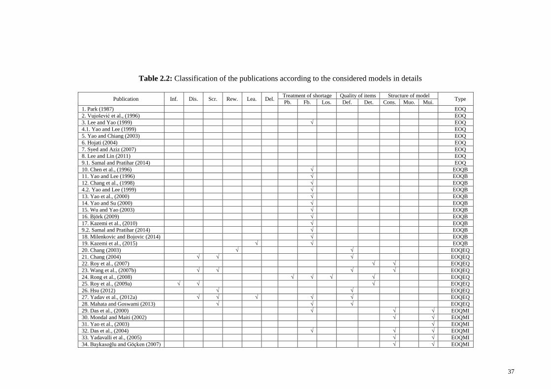
37

Table 2.2: Classification of the publications according to the considered models in details

Publication Inf. Dis. Scr. Rew. Lea. Del. Treatment of shortage Quality of items Structure of model

Type Pb. Fb. Los. Def. Det. Cons. Muo. Mui.

1. Park (1987) EOQ

2. Vujošević et al., (1996) EOQ

3. Lee and Yao (1999) √ EOQ

4.1. Yao and Lee (1999) EOQ

5. Yao and Chiang (2003) EOQ

6. Hojati (2004) EOQ

7. Syed and Aziz (2007) EOQ

8. Lee and Lin (2011) EOQ

9.1. Samal and Pratihar (2014) EOQ

10. Chen et al., (1996) √ EOQB

11. Yao and Lee (1996) √ EOQB

12. Chang et al., (1998) √ EOQB

4.2. Yao and Lee (1999) √ EOQB

13. Yao et al., (2000) √ EOQB

14. Yao and Su (2000) √ EOQB

15. Wu and Yao (2003) √ EOQB

16. Björk (2009) √ EOQB

17. Kazemi et al., (2010) √ EOQB

9.2. Samal and Pratihar (2014) √ EOQB

18. Milenkovic and Bojovic (2014) √ EOQB

19. Kazemi et al., (2015) √ √ EOQB

20. Chang (2003) √ √ EOQEQ

21. Chang (2004) √ √ √ EOQEQ

22. Roy et al., (2007) √ √ EOQEQ

23. Wang et al., (2007b) √ √ √ √ EOQEQ

24. Rong et al., (2008) √ √ √ √ EOQEQ

25. Roy et al., (2009a) √ √ √ EOQEQ

26. Hsu (2012) √ √ EOQEQ

27. Yadav et al., (2012a) √ √ √ √ √ EOQEQ

28. Mahata and Goswami (2013) √ √ √ EOQEQ

29. Das et al., (2000) √ √ √ EOQMI

30. Mondal and Maiti (2002) √ √ EOQMI

31. Yao et al., (2003) √ EOQMI

32. Das et al., (2004) √ √ √ EOQMI

33. Yadavalli et al., (2005) √ √ EOQMI

34. Baykasoğlu and Göçken (2007) √ √ EOQMI

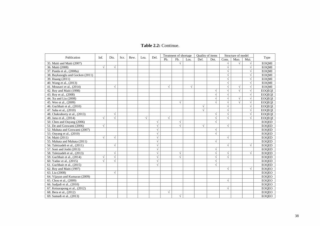
38




35. Maiti and Maiti (2007) √ √ √ √ EOQMI

36. Maiti (2008) √ √ √ √ EOQMI

37. Panda et al., (2008a) √ √ EOQMI

38. Baykasoglu and Gocken (2011) √ √ EOQMI

39. Huang (2011) √ √ EOQMI

40. Wang et al., (2013) √ √ EOQMI

41. Mousavi et al., (2014) √ √ √ √ √ √ EOQMI

42. Roy and Maiti (1998) √ √ √ √ EOQEQI

43. Roy et al., (2008) √ √ √ EOQEQI

44. Xu and Liu (2008) √ √ √ √ EOQEQI

45. Wee et al., (2009) √ √ √ √ √ EOQEQI

46. Guchhait et al., (2010) √ √ √ EOQEQI

47. Saha et al., (2010) √ √ √ EOQEQI

48. Chakraborty et al., (2013) √ √ √ √ EOQEQI

49. Jana et al., (2014) √ √ √ √ √ √ √ EOQEQI

50. Chen and Ouyang (2006) √ √ √ EOQED

51. De and Goswami (2006) √ √ √ √ √ EOQED

52. Mahata and Goswami (2007) √ √ EOQED

53. Ouyang et al., (2010) √ √ EOQED

54. Maiti (2011) √ √ √ √ EOQED

55. Mahata and Mahata (2011) √ √ EOQED

56. Taleizadeh et al., (2011) √ √ √ √ EOQED

57. Soni and Joshi (2013) √ √ EOQED

58. Taleizadeh et al., (2013) √ √ √ √ √ √ EOQED

59. Guchhait et al., (2014) √ √ √ √ √ √ EOQED

60. Yadav et al., (2015) √ √ √ √ EOQED

61. Guchhait et al., (2015) √ √ EOQED

62. Roy and Maiti (1997) √ √ EOQEO

63. Liu (2008) √ EOQEO

64. Vijayan and Kumaran (2009) EOQEO

65. Chou et al., (2009) √ EOQEO

66. Sadjadi et al., (2010) EOQEO

67. Ketsarapong et al., (2012) √ EOQEO

68. Bera et al., (2012) √ EOQEO

69. Samadi et al., (2013) √ EOQEO

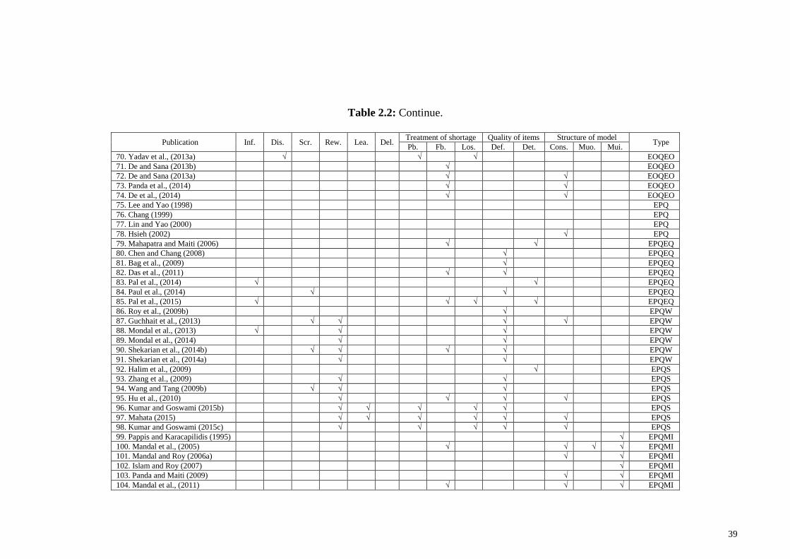
39




70. Yadav et al., (2013a) √ √ √ EOQEO

71. De and Sana (2013b) √ EOQEO

72. De and Sana (2013a) √ √ EOQEO

73. Panda et al., (2014) √ √ EOQEO

74. De et al., (2014) √ √ EOQEO

75. Lee and Yao (1998) EPQ

76. Chang (1999) EPQ

77. Lin and Yao (2000) EPQ

78. Hsieh (2002) √ EPQ

79. Mahapatra and Maiti (2006) √ √ EPQEQ

80. Chen and Chang (2008) √ EPQEQ

81. Bag et al., (2009) √ EPQEQ

82. Das et al., (2011) √ √ EPQEQ

83. Pal et al., (2014) √ √ EPQEQ

84. Paul et al., (2014) √ √ EPQEQ

85. Pal et al., (2015) √ √ √ √ EPQEQ

86. Roy et al., (2009b) √ EPQW

87. Guchhait et al., (2013) √ √ √ √ EPQW

88. Mondal et al., (2013) √ √ √ EPQW

89. Mondal et al., (2014) √ √ EPQW

90. Shekarian et al., (2014b) √ √ √ √ EPQW

91. Shekarian et al., (2014a) √ √ EPQW

92. Halim et al., (2009) √ EPQS

93. Zhang et al., (2009) √ √ EPQS

94. Wang and Tang (2009b) √ √ √ EPQS

95. Hu et al., (2010) √ √ √ √ EPQS

96. Kumar and Goswami (2015b) √ √ √ √ √ EPQS

97. Mahata (2015) √ √ √ √ √ √ EPQS

98. Kumar and Goswami (2015c) √ √ √ √ √ EPQS

99. Pappis and Karacapilidis (1995) √ EPQMI

100. Mandal et al., (2005) √ √ √ √ EPQMI

101. Mandal and Roy (2006a) √ √ EPQMI

102. Islam and Roy (2007) √ EPQMI

103. Panda and Maiti (2009) √ √ EPQMI

104. Mandal et al., (2011) √ √ √ EPQMI

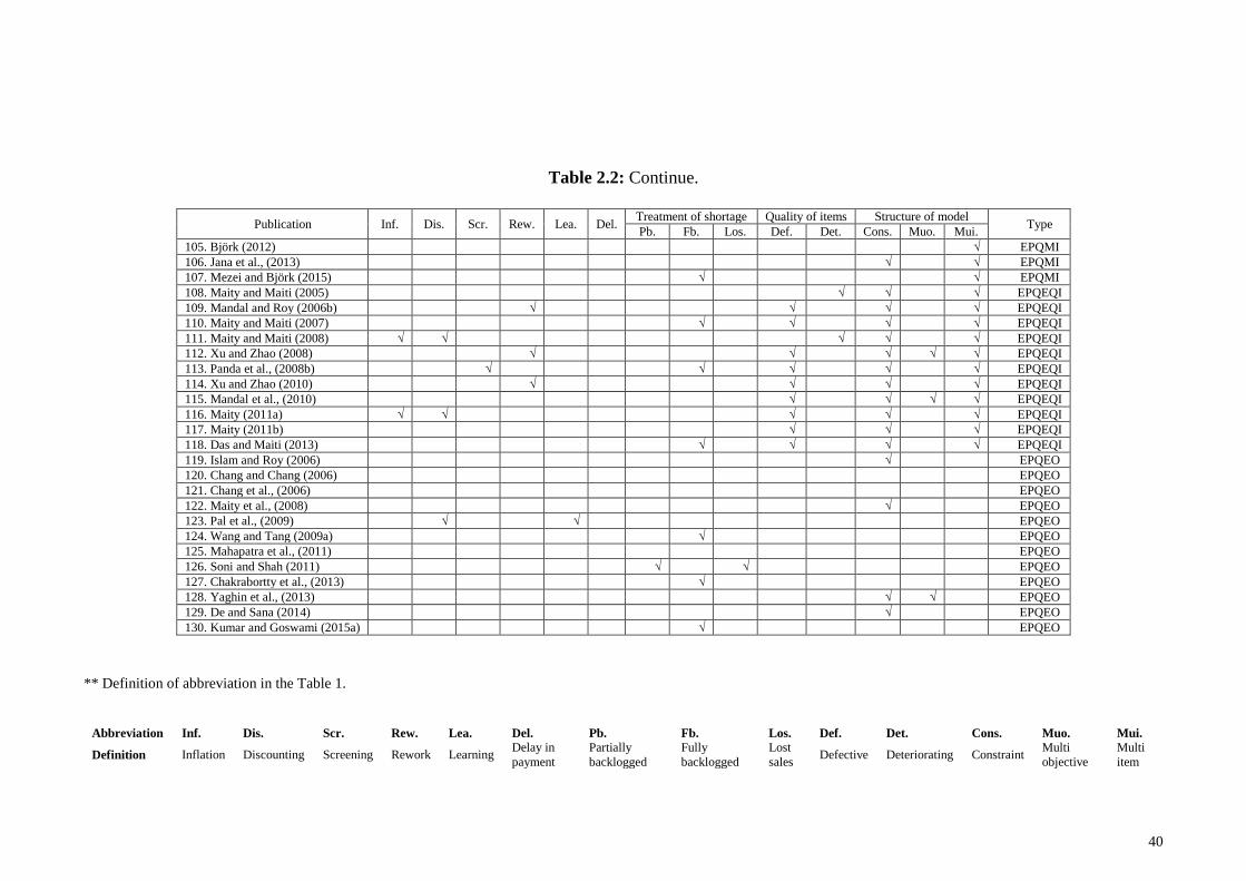
40




105. Björk (2012) √ EPQMI

106. Jana et al., (2013) √ √ EPQMI

107. Mezei and Björk (2015) √ √ EPQMI

108. Maity and Maiti (2005) √ √ √ EPQEQI

109. Mandal and Roy (2006b) √ √ √ √ EPQEQI

110. Maity and Maiti (2007) √ √ √ √ EPQEQI

111. Maity and Maiti (2008) √ √ √ √ √ EPQEQI

112. Xu and Zhao (2008) √ √ √ √ √ EPQEQI

113. Panda et al., (2008b) √ √ √ √ √ EPQEQI

114. Xu and Zhao (2010) √ √ √ √ EPQEQI

115. Mandal et al., (2010) √ √ √ √ EPQEQI

116. Maity (2011a) √ √ √ √ √ EPQEQI

117. Maity (2011b) √ √ √ EPQEQI

118. Das and Maiti (2013) √ √ √ √ EPQEQI

119. Islam and Roy (2006) √ EPQEO

120. Chang and Chang (2006) EPQEO

121. Chang et al., (2006) EPQEO

122. Maity et al., (2008) √ EPQEO

123. Pal et al., (2009) √ √ EPQEO

124. Wang and Tang (2009a) √ EPQEO

125. Mahapatra et al., (2011) EPQEO

126. Soni and Shah (2011) √ √ EPQEO

127. Chakrabortty et al., (2013) √ EPQEO

128. Yaghin et al., (2013) √ √ EPQEO

129. De and Sana (2014) √ EPQEO

130. Kumar and Goswami (2015a) √ EPQEO

** Definition of abbreviation in the Table 1.

Abbreviation Inf. Dis. Scr. Rew. Lea. Del. Pb. Fb. Los. Def. Det. Cons. Muo. Mui.

Definition Inflation Discounting Screening Rework Learning Delay in

payment

Partially

backlogged

Fully

backlogged

Lost

sales Defective Deteriorating Constraint

Multi

objective

Multi

item

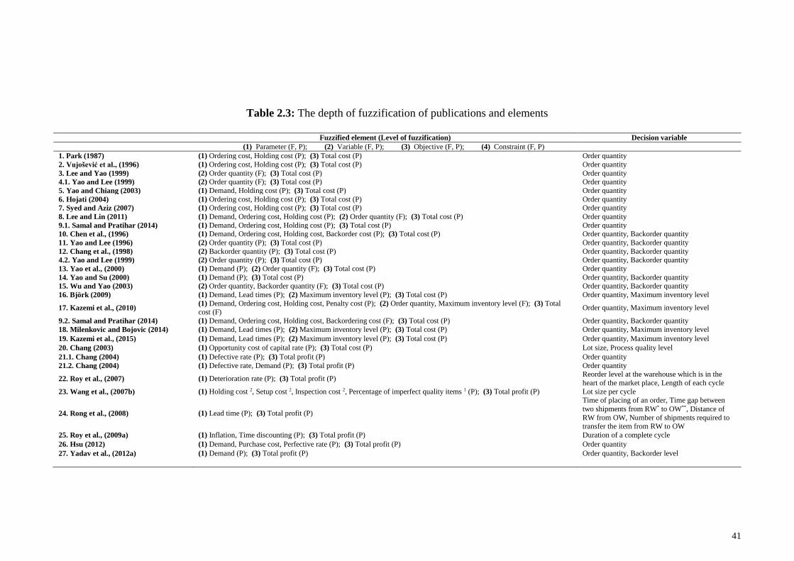
41

Table 2.3: The depth of fuzzification of publications and elements

Fuzzified element (Level of fuzzification) Decision variable

(1) Parameter (F, P); (2) Variable (F, P); (3) Objective (F, P); (4) Constraint (F, P)

1. Park (1987) (1) Ordering cost, Holding cost (P); (3) Total cost (P) Order quantity

2. Vujošević et al., (1996) (1) Ordering cost, Holding cost (P); (3) Total cost (P) Order quantity

3. Lee and Yao (1999) (2) Order quantity (F); (3) Total cost (P) Order quantity

4.1. Yao and Lee (1999) (2) Order quantity (F); (3) Total cost (P) Order quantity

5. Yao and Chiang (2003) (1) Demand, Holding cost (P); (3) Total cost (P) Order quantity

6. Hojati (2004) (1) Ordering cost, Holding cost (P); (3) Total cost (P) Order quantity

7. Syed and Aziz (2007) (1) Ordering cost, Holding cost (P); (3) Total cost (P) Order quantity

8. Lee and Lin (2011) (1) Demand, Ordering cost, Holding cost (P); (2) Order quantity (F); (3) Total cost (P) Order quantity

9.1. Samal and Pratihar (2014) (1) Demand, Ordering cost, Holding cost (P); (3) Total cost (P) Order quantity

10. Chen et al., (1996) (1) Demand, Ordering cost, Holding cost, Backorder cost (P); (3) Total cost (P) Order quantity, Backorder quantity

11. Yao and Lee (1996) (2) Order quantity (P); (3) Total cost (P) Order quantity, Backorder quantity

12. Chang et al., (1998) (2) Backorder quantity (P); (3) Total cost (P) Order quantity, Backorder quantity

4.2. Yao and Lee (1999) (2) Order quantity (P); (3) Total cost (P) Order quantity, Backorder quantity

13. Yao et al., (2000) (1) Demand (P); (2) Order quantity (F); (3) Total cost (P) Order quantity

14. Yao and Su (2000) (1) Demand (P); (3) Total cost (P) Order quantity, Backorder quantity

15. Wu and Yao (2003) (2) Order quantity, Backorder quantity (F); (3) Total cost (P) Order quantity, Backorder quantity

16. Björk (2009) (1) Demand, Lead times (P); (2) Maximum inventory level (P); (3) Total cost (P) Order quantity, Maximum inventory level

17. Kazemi et al., (2010) (1) Demand, Ordering cost, Holding cost, Penalty cost (P); (2) Order quantity, Maximum inventory level (F); (3) Total cost (F)

Order quantity, Maximum inventory level

9.2. Samal and Pratihar (2014) (1) Demand, Ordering cost, Holding cost, Backordering cost (F); (3) Total cost (P) Order quantity, Backorder quantity

18. Milenkovic and Bojovic (2014) (1) Demand, Lead times (P); (2) Maximum inventory level (P); (3) Total cost (P) Order quantity, Maximum inventory level

19. Kazemi et al., (2015) (1) Demand, Lead times (P); (2) Maximum inventory level (P); (3) Total cost (P) Order quantity, Maximum inventory level

20. Chang (2003) (1) Opportunity cost of capital rate (P); (3) Total cost (P) Lot size, Process quality level

21.1. Chang (2004) (1) Defective rate (P); (3) Total profit (P) Order quantity

21.2. Chang (2004) (1) Defective rate, Demand (P); (3) Total profit (P) Order quantity

22. Roy et al., (2007) (1) Deterioration rate (P); (3) Total profit (P) Reorder level at the warehouse which is in the

heart of the market place, Length of each cycle

23. Wang et al., (2007b) (1) Holding cost 2, Setup cost 2, Inspection cost 2, Percentage of imperfect quality items 1 (P); (3) Total profit (P) Lot size per cycle

24. Rong et al., (2008) (1) Lead time (P); (3) Total profit (P)

Time of placing of an order, Time gap between

two shipments from RW* to OW**, Distance of

RW from OW, Number of shipments required to transfer the item from RW to OW

25. Roy et al., (2009a) (1) Inflation, Time discounting (P); (3) Total profit (P) Duration of a complete cycle

26. Hsu (2012) (1) Demand, Purchase cost, Perfective rate (P); (3) Total profit (P) Order quantity

27. Yadav et al., (2012a) (1) Demand (P); (3) Total profit (P) Order quantity, Backorder level

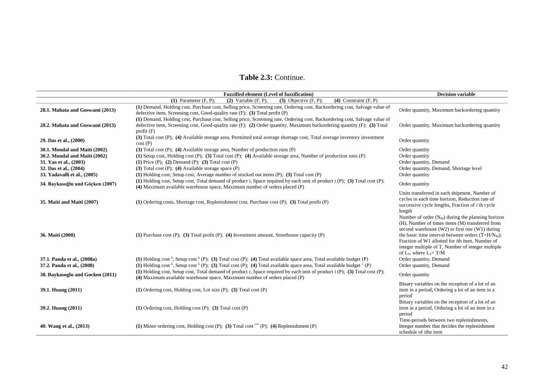
42




28.1. Mahata and Goswami (2013) (1) Demand, Holding cost, Purchase cost, Selling price, Screening rate, Ordering cost, Backordering cost, Salvage value of defective item, Screening cost, Good-quality rate (F); (3) Total profit (P)

Order quantity, Maximum backordering quantity

28.2. Mahata and Goswami (2013)

(1) Demand, Holding cost, Purchase cost, Selling price, Screening rate, Ordering cost, Backordering cost, Salvage value of

defective item, Screening cost, Good-quality rate (F); (2) Order quantity, Maximum backordering quantity (F); (3) Total profit (F)

Order quantity, Maximum backordering quantity

29. Das et al., (2000) (3) Total cost (P); (4) Available storage area, Permitted total average shortage cost, Total average inventory investment

cost (P) Order quantity

30.1. Mondal and Maiti (2002) (3) Total cost (P); (4) Available storage area, Number of production runs (P) Order quantity

30.2. Mondal and Maiti (2002) (1) Setup cost, Holding cost (P); (3) Total cost (P); (4) Available storage area, Number of production runs (P) Order quantity

31. Yao et al., (2003) (1) Price (P); (2) Demand (P); (3) Total cost (P) Order quantity, Demand

32. Das et al., (2004) (3) Total cost (P); (4) Available storage space (P) Order quantity, Demand, Shortage level

33. Yadavalli et al., (2005) (1) Holding cost; Setup cost, Average number of stocked out items (P); (3) Total cost (P) Order quantity

34. Baykasoğlu and Göçken (2007) (1) Holding cost, Setup cost, Total demand of product i, Space required by each unit of product i (P); (3) Total cost (P);

(4) Maximum available warehouse space, Maximum number of orders placed (P) Order quantity

35. Maiti and Maiti (2007) (1) Ordering costs, Shortage cost, Replenishment cost, Purchase cost (P); (3) Total profit (P)

Units transferred in each shipment, Number of

cycles in each time horizon, Reduction rate of

successive cycle lengths, Fraction of i th cycle length

36. Maiti (2008) (1) Purchase cost (P); (3) Total profit (P); (4) Investment amount, Storehouse capacity (P)

Number of order (NM) during the planning horizon

(H), Number of times items (M) transferred from

second warehouse (W2) to first one (W1) during the basic time interval between orders (T=H/NM);

Fraction of W1 allotted for ith item, Number of integer multiple of T, Number of integer multiple

of LT, where LT= T/M

37.1. Panda et al., (2008a) (1) Holding cost 6, Setup cost 6 (P); (3) Total cost (P); (4) Total available space area, Total available budget (P) Order quantity, Demand

37.2. Panda et al., (2008) (1) Holding cost 6, Setup cost 6 (P); (3) Total cost (P); (4) Total available space area, Total available budget 1 (P) Order quantity, Demand

38. Baykasoglu and Gocken (2011) (1) Holding cost, Setup cost, Total demand of product i, Space required by each unit of product i (P); (3) Total cost (P); (4) Maximum available warehouse space, Maximum number of orders placed (P)

Order quantity

39.1. Huang (2011) (1) Ordering cost, Holding cost, Lot size (P); (3) Total cost (P)

Binary variables on the reception of a lot of an

item in a period, Ordering a lot of an item in a period

39.2. Huang (2011) (1) Ordering cost, Holding cost (P); (3) Total cost (P)

Binary variables on the reception of a lot of an

item in a period, Ordering a lot of an item in a

period

40. Wang et al., (2013) (1) Minor ordering cost, Holding cost (P); (3) Total cost *** (P); (4) Replenishment (P)

Time-periods between two replenishments,

Integer number that decides the replenishment

schedule of ithe item

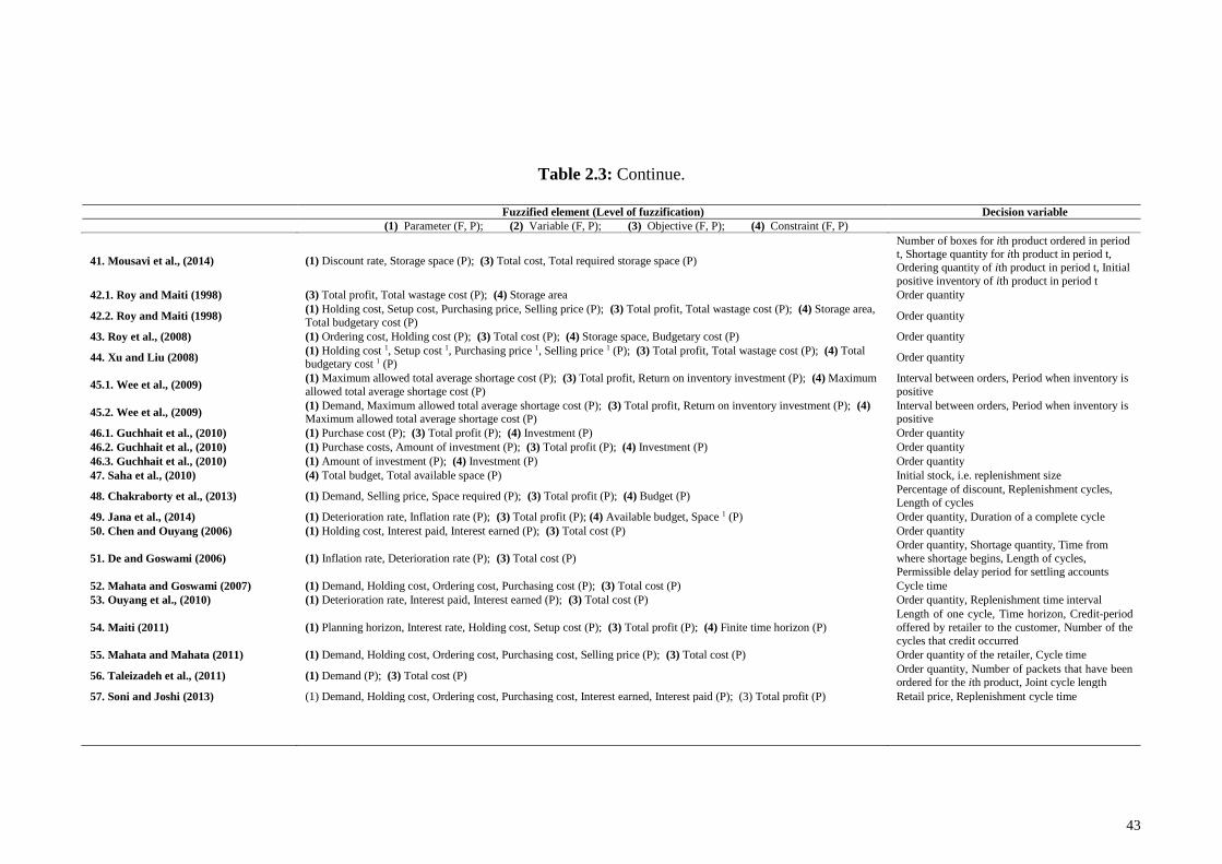
43




41. Mousavi et al., (2014) (1) Discount rate, Storage space (P); (3) Total cost, Total required storage space (P)

Number of boxes for ith product ordered in period t, Shortage quantity for ith product in period t,

Ordering quantity of ith product in period t, Initial

positive inventory of ith product in period t

42.1. Roy and Maiti (1998) (3) Total profit, Total wastage cost (P); (4) Storage area Order quantity

42.2. Roy and Maiti (1998) (1) Holding cost, Setup cost, Purchasing price, Selling price (P); (3) Total profit, Total wastage cost (P); (4) Storage area,

Total budgetary cost (P) Order quantity

43. Roy et al., (2008) (1) Ordering cost, Holding cost (P); (3) Total cost (P); (4) Storage space, Budgetary cost (P) Order quantity

44. Xu and Liu (2008) (1) Holding cost 1, Setup cost 1, Purchasing price 1, Selling price 1 (P); (3) Total profit, Total wastage cost (P); (4) Total budgetary cost 1 (P)

Order quantity

45.1. Wee et al., (2009) (1) Maximum allowed total average shortage cost (P); (3) Total profit, Return on inventory investment (P); (4) Maximum

allowed total average shortage cost (P)

Interval between orders, Period when inventory is

positive

45.2. Wee et al., (2009) (1) Demand, Maximum allowed total average shortage cost (P); (3) Total profit, Return on inventory investment (P); (4)

Maximum allowed total average shortage cost (P) Interval between orders, Period when inventory is positive

46.1. Guchhait et al., (2010) (1) Purchase cost (P); (3) Total profit (P); (4) Investment (P) Order quantity

46.2. Guchhait et al., (2010) (1) Purchase costs, Amount of investment (P); (3) Total profit (P); (4) Investment (P) Order quantity

46.3. Guchhait et al., (2010) (1) Amount of investment (P); (4) Investment (P) Order quantity

47. Saha et al., (2010) (4) Total budget, Total available space (P) Initial stock, i.e. replenishment size

48. Chakraborty et al., (2013) (1) Demand, Selling price, Space required (P); (3) Total profit (P); (4) Budget (P) Percentage of discount, Replenishment cycles,

Length of cycles

49. Jana et al., (2014) (1) Deterioration rate, Inflation rate (P); (3) Total profit (P); (4) Available budget, Space 1 (P) Order quantity, Duration of a complete cycle

50. Chen and Ouyang (2006) (1) Holding cost, Interest paid, Interest earned (P); (3) Total cost (P) Order quantity

51. De and Goswami (2006) (1) Inflation rate, Deterioration rate (P); (3) Total cost (P)

Order quantity, Shortage quantity, Time from

where shortage begins, Length of cycles,

Permissible delay period for settling accounts

52. Mahata and Goswami (2007) (1) Demand, Holding cost, Ordering cost, Purchasing cost (P); (3) Total cost (P) Cycle time

53. Ouyang et al., (2010) (1) Deterioration rate, Interest paid, Interest earned (P); (3) Total cost (P) Order quantity, Replenishment time interval

54. Maiti (2011) (1) Planning horizon, Interest rate, Holding cost, Setup cost (P); (3) Total profit (P); (4) Finite time horizon (P)

Length of one cycle, Time horizon, Credit-period

offered by retailer to the customer, Number of the

cycles that credit occurred

55. Mahata and Mahata (2011) (1) Demand, Holding cost, Ordering cost, Purchasing cost, Selling price (P); (3) Total cost (P) Order quantity of the retailer, Cycle time

56. Taleizadeh et al., (2011) (1) Demand (P); (3) Total cost (P) Order quantity, Number of packets that have been

ordered for the ith product, Joint cycle length

57. Soni and Joshi (2013) (1) Demand, Holding cost, Ordering cost, Purchasing cost, Interest earned, Interest paid (P); (3) Total profit (P) Retail price, Replenishment cycle time

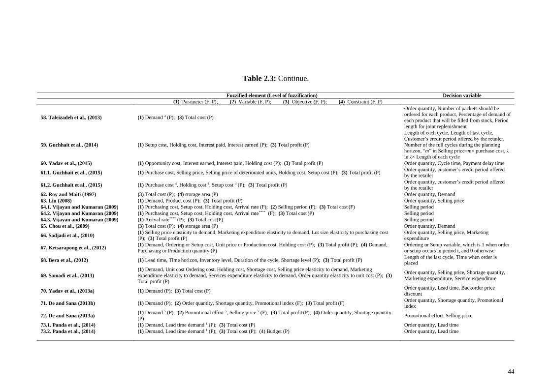
44




58. Taleizadeh et al., (2013) (1) Demand 4 (P); (3) Total cost (P)

Order quantity, Number of packets should be ordered for each product, Percentage of demand of

each product that will be filled from stock, Period

length for joint replenishment

59. Guchhait et al., (2014) (1) Setup cost, Holding cost, Interest paid, Interest earned (P); (3) Total profit (P)

Length of each cycle, Length of last cycle,

Customer’s credit period offered by the retailer,

Number of the full cycles during the planning horizon, “m” in Selling price=m× purchase cost, λ

in λ× Length of each cycle

60. Yadav et al., (2015) (1) Opportunity cost, Interest earned, Interest paid, Holding cost (P); (3) Total profit (P) Order quantity, Cycle time, Payment delay time

61.1. Guchhait et al., (2015) (1) Purchase cost, Selling price, Selling price of deteriorated units, Holding cost, Setup cost (P); (3) Total profit (P) Order quantity, customer’s credit period offered by the retailer

61.2. Guchhait et al., (2015) (1) Purchase cost 4, Holding cost 4, Setup cost 4 (P); (3) Total profit (P) Order quantity, customer’s credit period offered

by the retailer

62. Roy and Maiti (1997) (3) Total cost (P); (4) storage area (P) Order quantity, Demand

63. Liu (2008) (1) Demand, Product cost (P); (3) Total profit (P) Order quantity, Selling price

64.1. Vijayan and Kumaran (2009) (1) Purchasing cost, Setup cost, Holding cost, Arrival rate (F); (2) Selling period (F); (3) Total cost (F) Selling period

64.2. Vijayan and Kumaran (2009) (1) Purchasing cost, Setup cost, Holding cost, Arrival rate**** (F); (3) Total cost (P) Selling period

64.3. Vijayan and Kumaran (2009) (1) Arrival rate**** (P); (3) Total cost (P) Selling period

65. Chou et al., (2009) (3) Total cost (P); (4) storage area (P) Order quantity, Demand

66. Sadjadi et al., (2010) (1) Selling price elasticity to demand, Marketing expenditure elasticity to demand, Lot size elasticity to purchasing cost (P); (3) Total profit (P)

Order quantity, Selling price, Marketing expenditure

67. Ketsarapong et al., (2012) (1) Demand, Ordering or Setup cost, Unit price or Production cost, Holding cost (P); (3) Total profit (P); (4) Demand,

Purchasing or Production quantity (P)

Ordering or Setup variable, which is 1 when order

or setup occurs in period t, and 0 otherwise

68. Bera et al., (2012) (1) Lead time, Time horizon, Inventory level, Duration of the cycle, Shortage level (P); (3) Total profit (P) Length of the last cycle, Time when order is placed

69. Samadi et al., (2013)

(1) Demand, Unit cost Ordering cost, Holding cost, Shortage cost, Selling price elasticity to demand, Marketing

expenditure elasticity to demand, Services expenditure elasticity to demand, Order quantity elasticity to unit cost (P); (3) Total profit (P)

Order quantity, Selling price, Shortage quantity,

Marketing expenditure, Service expenditure

70. Yadav et al., (2013a) (1) Demand (P); (3) Total cost (P) Order quantity, Lead time, Backorder price

discount

71. De and Sana (2013b) (1) Demand (P); (2) Order quantity, Shortage quantity, Promotional index (F); (3) Total profit (F) Order quantity, Shortage quantity, Promotional index

72. De and Sana (2013a) (1) Demand 5 (P); (2) Promotional effort 5, Selling price 5 (F); (3) Total profit (P); (4) Order quantity, Shortage quantity

(P) Promotional effort, Selling price

73.1. Panda et al., (2014) (1) Demand, Lead time demand 1 (P); (3) Total cost (P) Order quantity, Lead time

73.2. Panda et al., (2014) (1) Demand, Lead time demand 1 (P); (3) Total cost (P); (4) Budget (P) Order quantity, Lead time

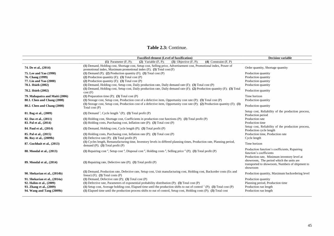
45




74. De et al., (2014) (1) Demand, Holding cost, Shortage cost, Setup cost, Selling price, Advertisement cost, Promotional index, Power of promotional index, Maximum promotional index (F); (3) Total cost (F)

Order quantity, Shortage quantity

75. Lee and Yao (1998) (1) Demand (P); (2) Production quantity (F); (3) Total cost (P) Production quantity

76. Chang (1999) (2) Production quantity (F); (3) Total cost (P) Production quantity

77. Lin and Yao (2000) (2) Production quantity (F); (3) Total cost (P) Production quantity

78.1. Hsieh (2002) (1) Demand, Holding cost, Setup cost, Daily production rate, Daily demand rate (F); (3) Total cost (P) Production quantity

78.2. Hsieh (2002) (1) Demand, Holding cost, Setup cost, Daily production rate, Daily demand rate (F); (2) Production quantity (F); (3) Total

cost (F) Production quantity

79. Mahapatra and Maiti (2006) (1) Preparation time (P); (3) Total cost (P) Time horizon

80.1. Chen and Chang (2008) (1) Storage cost, Setup cost, Production cost of a defective item, Opportunity cost rate (P); (3) Total cost (P) Production quantity

80.2. Chen and Chang (2008) (1) Storage cost, Setup cost, Production cost of a defective item, Opportunity cost rate (P); (2) Production quantity (F); (3) Total cost (P)

Production quantity

81. Bag et al., (2009) (1) Demand 1, Cycle length 1 (P); (3) Total profit (P) Setup cost, Reliability of the production process,

Production period

82. Das et al., (2011) (1) Holding cost, Shortage cost, Coefficients in production cost functions (P); (3) Total profit (P) Production rate

83. Pal et al., (2014) (1) Holding costs, Purchasing cost, Inflation rate (P); (3) Total cost (P) Production time

84. Paul et al., (2014) (1) Demand, Holding cost, Cycle length (P); (3) Total profit (P) Setup cost, Reliability of the production process,

Production cycle length

85. Pal et al., (2015) (1) Holding costs, Purchasing cost, Inflation rate (P); (3) Total cost (P) Production time, Production rate

86. Roy et al., (2009b) (1) Defective rate (P); (3) Total profit (P) Cycle length

87. Guchhait et al., (2013) (1) Cycles length, Remanufacturing time, Inventory levels in differed planning times, Production rate, Planning period,

demand (P); (3) Total profit (P) Time horizon

88. Mondal et al., (2013) (1) Repairing cost 4, Setup cost 4, Disposal cost 4, Holding costs 4, Selling price 4 (P); (3) Total profit (P) Production function’s coefficients, Repairing function’s coefficients

89. Mondal et al., (2014) (1) Repairing rate, Defective rate (P); (3) Total profit (P)

Production rate, Minimum inventory level at

showroom, The period which the units are

transported to showroom, Numbers of shipment to showroom

90. Shekarian et al., (2014b) (1) Demand, Production rate, Defective rate, Setup cost, Unit manufacturing cost, Holding cost, Backorder costs (fix and

linear) (F); (3) Total costs (P) Production quantity, Maximum backordering level

91. Shekarian et al., (2014a) (1) Demand, Defective rate (P); (3) Total cost (P) Production quantity

92. Halim et al., (2009) (1) Defective rate, Parameters of exponential probability distribution (P); (3) Total cost (P) Planning period, Production time

93. Zhang et al., (2009) (1) Setup cost, Average holding cost, Elapsed time until the production shifts to out of control 1 (P); (3) Total cost (P) Production run length

94. Wang and Tang (2009b) (1) Elapsed time until the production process shifts to out of control, Setup cost, Holding costs (P); (3) Total cost Production run length

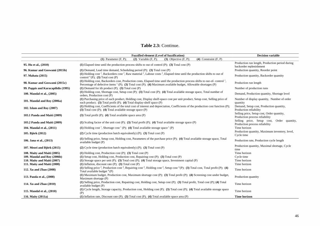
46




95. Hu et al., (2010) (1) Elapsed time until the production process shifts to out of control (P); (3) Total cost (P) Production run length, Production period during backorder replenishment

96. Kumar and Goswami (2015b) (1) Demand, Lead time demand, Scheduling period (P); (3) Total cost (P) Production quantity, Reorder point

97. Mahata (2015) (1) Holding cost 2, Backorders cost 2, Raw material 2, Labour costs 2, Elapsed time until the production shifts to out of

control 4 (P); (3) Total cost (P) Production quantity, Backorder quantity

98. Kumar and Goswami (2015c) (1) Holding cost, Backorders cost, Production costs, Elapsed time until the production process shifts to out-of- control 1,

Percentage of defective items 1 (P); (3) Total cost (P); (4) Maximum available budget, Allowable shortages (P) Production run length

99. Pappis and Karacapilidis (1995) (1) Demand for ith product (P); (3) Total cost (P) Number of production runs

100. Mandal et al., (2005) (1) Holding cost, Shortage cost, Setup cost (P); (3) Total cost (P); (4) Total available storage space, Total number of orders, Production cost (P)

Demand, Production quantity, Shortage level

101. Mandal and Roy (2006a) (1) Purchasing price of each product, Holding cost, Display shelf-space cost per unit product, Setup cost, Selling price of

each product; (3) Total profit (P); (4) Total display-shelf space (P)

Number of display quantity, Number of order

quantity

102. Islam and Roy (2007) (1) Holding cost, Coefficients of the total cost of interest and depreciation, Coefficients of the production cost function (P); (3) Total cost (P); (4) Total available storage space (P)

Demand, Setup cost, Production quantity, Production reliability

103.1 Panda and Maiti (2009) (3) Total profit (P); (4) Total available space area (P) Selling price, Setup cost, Order quantity,

Production process reliability

103.2 Panda and Maiti (2009) (1) Scaling factor of the unit cost (P); (3) Total profit (P); (4) Total available storage space (P) Selling price, Setup cost, Order quantity, Production process reliability

104. Mandal et al., (2011) (1) Holding cost 1, Shortage cost 1 (P); (4) Total available storage space 1 (P) Time horizon

105. Björk (2012) (2) Cycle time (production batch equivalently) (P); (3) Total cost (P) Production quantity, Maximum inventory, level,

Cycle time

106. Jana et al., (2013) (1) Selling price, Setup cost, Holding cost, Parameters of the purchase price (P); (4) Total available storage space, Total available budget (P)

Production rate, Production cycle length

107. Mezei and Björk (2015) (2) Cycle time (production batch equivalently) (P); (3) Total cost (P) Production quantity, Maximal shortage, Cycle

time

108. Maity and Maiti (2005) (1) Holding cost, Production cost (P); (3) Total cost (P) Time horizon

109. Mandal and Roy (2006b) (1) Setup cost, Holding cost, Production cost, Repairing cost (P); (3) Total cost (P) Cycle time

110. Maity and Maiti (2007) (1) Storage space per unit (P); (3) Total cost (P); (4) Total storage space, Investment capital (P) Time horizon

111. Maity and Maiti (2008) (1) Inflation, discount rate (P); (3) Total cost (P) Time horizon

112. Xu and Zhao (2008) (1) Selling price 4, Production cost 4, Repairing cost 4, Holding cost 4, Setup cost 4 (P); (3) Total cost, Total profit (P); (4) Total available budget 4 (P)

Time horizon

113. Panda et al., (2008) (1) Maximum budget, Production cost, Maximum shortage cost (P); (3) Total profit (P); (4) Screening cost under budget,

Maximum shortage (P) Production quantity

114. Xu and Zhao (2010) (1) Selling price, Production cost, Repairing cost, Holding cost, Setup cost (P); (3) Total profit, Total cost (P); (4) Total available budget (P)

Time horizon

115. Mandal et al., (2010) (1) Cycle length, Storage capacity, Production cost, Holding cost (P); (3) Total cost (P); (4) Total available storage space

(P) Time horizon

116. Maity (2011a) (1) Inflation rate, Discount rate (P); (3) Total cost (P); (4) Total available space area (P) Time horizon

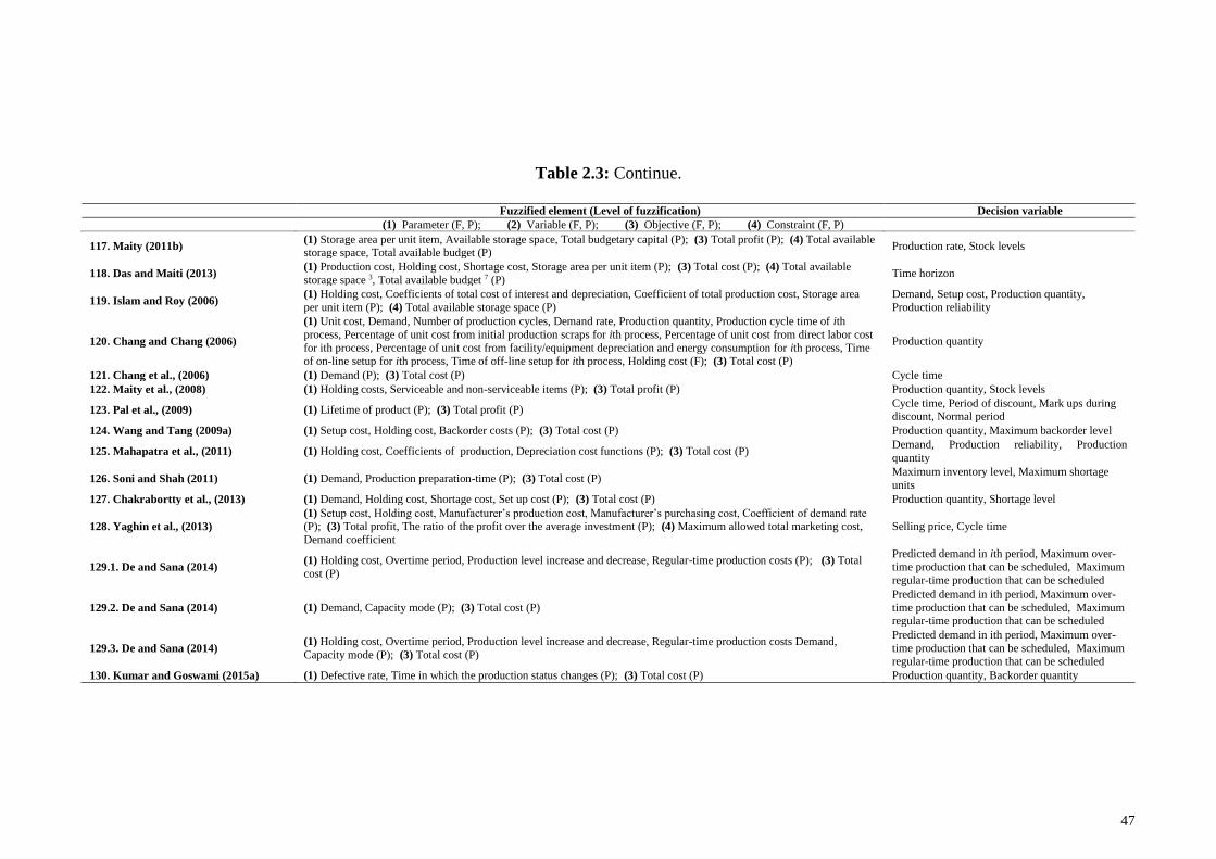
47




117. Maity (2011b) (1) Storage area per unit item, Available storage space, Total budgetary capital (P); (3) Total profit (P); (4) Total available storage space, Total available budget (P)

Production rate, Stock levels

118. Das and Maiti (2013) (1) Production cost, Holding cost, Shortage cost, Storage area per unit item (P); (3) Total cost (P); (4) Total available

storage space 3, Total available budget 7 (P) Time horizon

119. Islam and Roy (2006) (1) Holding cost, Coefficients of total cost of interest and depreciation, Coefficient of total production cost, Storage area per unit item (P); (4) Total available storage space (P)

Demand, Setup cost, Production quantity, Production reliability

120. Chang and Chang (2006)

(1) Unit cost, Demand, Number of production cycles, Demand rate, Production quantity, Production cycle time of ith

process, Percentage of unit cost from initial production scraps for ith process, Percentage of unit cost from direct labor cost for ith process, Percentage of unit cost from facility/equipment depreciation and energy consumption for ith process, Time

of on-line setup for ith process, Time of off-line setup for ith process, Holding cost (F); (3) Total cost (P)

Production quantity

121. Chang et al., (2006) (1) Demand (P); (3) Total cost (P) Cycle time

122. Maity et al., (2008) (1) Holding costs, Serviceable and non-serviceable items (P); (3) Total profit (P) Production quantity, Stock levels

123. Pal et al., (2009) (1) Lifetime of product (P); (3) Total profit (P) Cycle time, Period of discount, Mark ups during discount, Normal period

124. Wang and Tang (2009a) (1) Setup cost, Holding cost, Backorder costs (P); (3) Total cost (P) Production quantity, Maximum backorder level

125. Mahapatra et al., (2011) (1) Holding cost, Coefficients of production, Depreciation cost functions (P); (3) Total cost (P) Demand, Production reliability, Production

quantity

126. Soni and Shah (2011) (1) Demand, Production preparation-time (P); (3) Total cost (P) Maximum inventory level, Maximum shortage

units

127. Chakrabortty et al., (2013) (1) Demand, Holding cost, Shortage cost, Set up cost (P); (3) Total cost (P) Production quantity, Shortage level

128. Yaghin et al., (2013)

(1) Setup cost, Holding cost, Manufacturer’s production cost, Manufacturer’s purchasing cost, Coefficient of demand rate (P); (3) Total profit, The ratio of the profit over the average investment (P); (4) Maximum allowed total marketing cost,

Demand coefficient

Selling price, Cycle time

129.1. De and Sana (2014) (1) Holding cost, Overtime period, Production level increase and decrease, Regular-time production costs (P); (3) Total

cost (P)

Predicted demand in ith period, Maximum over-time production that can be scheduled, Maximum

regular-time production that can be scheduled

129.2. De and Sana (2014) (1) Demand, Capacity mode (P); (3) Total cost (P)

Predicted demand in ith period, Maximum over-

time production that can be scheduled, Maximum regular-time production that can be scheduled

129.3. De and Sana (2014) (1) Holding cost, Overtime period, Production level increase and decrease, Regular-time production costs Demand,

Capacity mode (P); (3) Total cost (P)

Predicted demand in ith period, Maximum over-

time production that can be scheduled, Maximum regular-time production that can be scheduled

130. Kumar and Goswami (2015a) (1) Defective rate, Time in which the production status changes (P); (3) Total cost (P) Production quantity, Backorder quantity

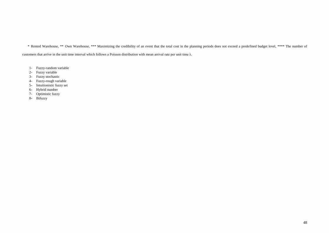
48

* Rented Warehouse, ** Own Warehouse, *** Maximizing the credibility of an event that the total cost in the planning periods does not exceed a predefined budget level, **** The number of

customers that arrive in the unit time interval which follows a Poisson distribution with mean arrival rate per unit time λ.

1- Fuzzy-random variable

2- Fuzzy variable

3- Fuzzy stochastic

4- Fuzzy-rough variable

5- Intuitionistic fuzzy set

6- Hybrid number

7- Optimistic fuzzy

8- Bifuzzy

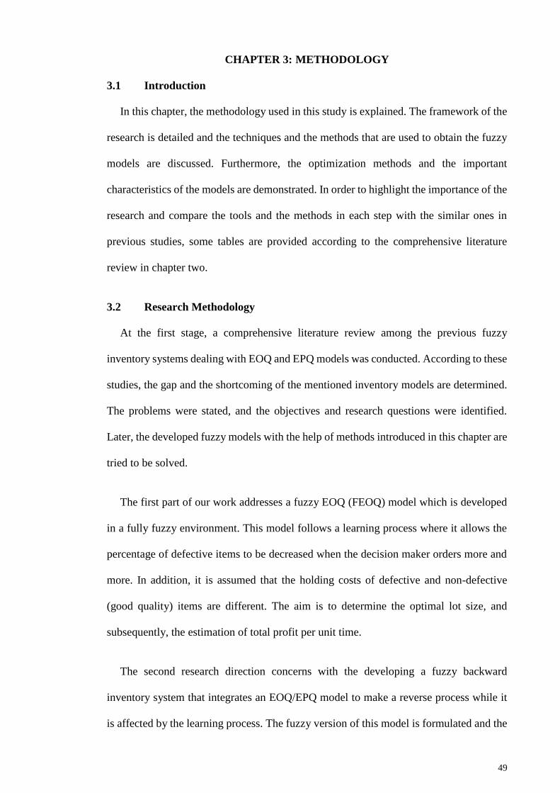
49

CHAPTER 3: METHODOLOGY

3.1 Introduction

In this chapter, the methodology used in this study is explained. The framework of the

research is detailed and the techniques and the methods that are used to obtain the fuzzy

models are discussed. Furthermore, the optimization methods and the important

characteristics of the models are demonstrated. In order to highlight the importance of the

research and compare the tools and the methods in each step with the similar ones in

previous studies, some tables are provided according to the comprehensive literature

review in chapter two.

3.2 Research Methodology

At the first stage, a comprehensive literature review among the previous fuzzy

inventory systems dealing with EOQ and EPQ models was conducted. According to these

studies, the gap and the shortcoming of the mentioned inventory models are determined.

The problems were stated, and the objectives and research questions were identified.

Later, the developed fuzzy models with the help of methods introduced in this chapter are

tried to be solved.

The first part of our work addresses a fuzzy EOQ (FEOQ) model which is developed

in a fully fuzzy environment. This model follows a learning process where it allows the

percentage of defective items to be decreased when the decision maker orders more and

more. In addition, it is assumed that the holding costs of defective and non-defective

(good quality) items are different. The aim is to determine the optimal lot size, and

subsequently, the estimation of total profit per unit time.

The second research direction concerns with the developing a fuzzy backward

inventory system that integrates an EOQ/EPQ model to make a reverse process while it

is affected by the learning process. The fuzzy version of this model is formulated and the

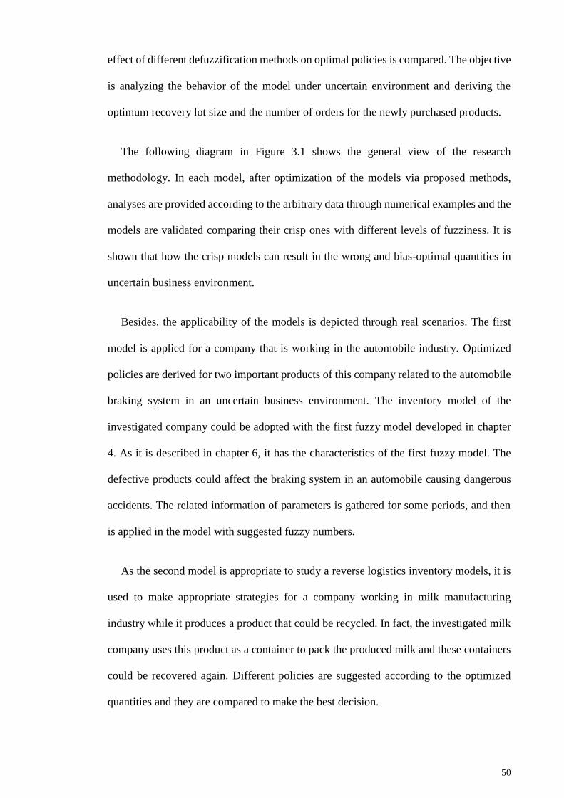
50

effect of different defuzzification methods on optimal policies is compared. The objective

is analyzing the behavior of the model under uncertain environment and deriving the

optimum recovery lot size and the number of orders for the newly purchased products.

The following diagram in Figure 3.1 shows the general view of the research

methodology. In each model, after optimization of the models via proposed methods,

analyses are provided according to the arbitrary data through numerical examples and the

models are validated comparing their crisp ones with different levels of fuzziness. It is

shown that how the crisp models can result in the wrong and bias-optimal quantities in

uncertain business environment.

Besides, the applicability of the models is depicted through real scenarios. The first

model is applied for a company that is working in the automobile industry. Optimized

policies are derived for two important products of this company related to the automobile

braking system in an uncertain business environment. The inventory model of the

investigated company could be adopted with the first fuzzy model developed in chapter

4. As it is described in chapter 6, it has the characteristics of the first fuzzy model. The

defective products could affect the braking system in an automobile causing dangerous

accidents. The related information of parameters is gathered for some periods, and then

is applied in the model with suggested fuzzy numbers.

As the second model is appropriate to study a reverse logistics inventory models, it is

used to make appropriate strategies for a company working in milk manufacturing

industry while it produces a product that could be recycled. In fact, the investigated milk

company uses this product as a container to pack the produced milk and these containers

could be recovered again. Different policies are suggested according to the optimized

quantities and they are compared to make the best decision.

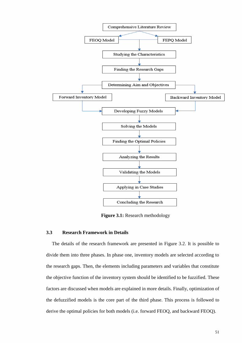
51

Figure 3.1: Research methodology

3.3 Research Framework in Details

The details of the research framework are presented in Figure 3.2. It is possible to

divide them into three phases. In phase one, inventory models are selected according to

the research gaps. Then, the elements including parameters and variables that constitute

the objective function of the inventory system should be identified to be fuzzified. These

factors are discussed when models are explained in more details. Finally, optimization of

the defuzzified models is the core part of the third phase. This process is followed to

derive the optimal policies for both models (i.e. forward FEOQ, and backward FEOQ).

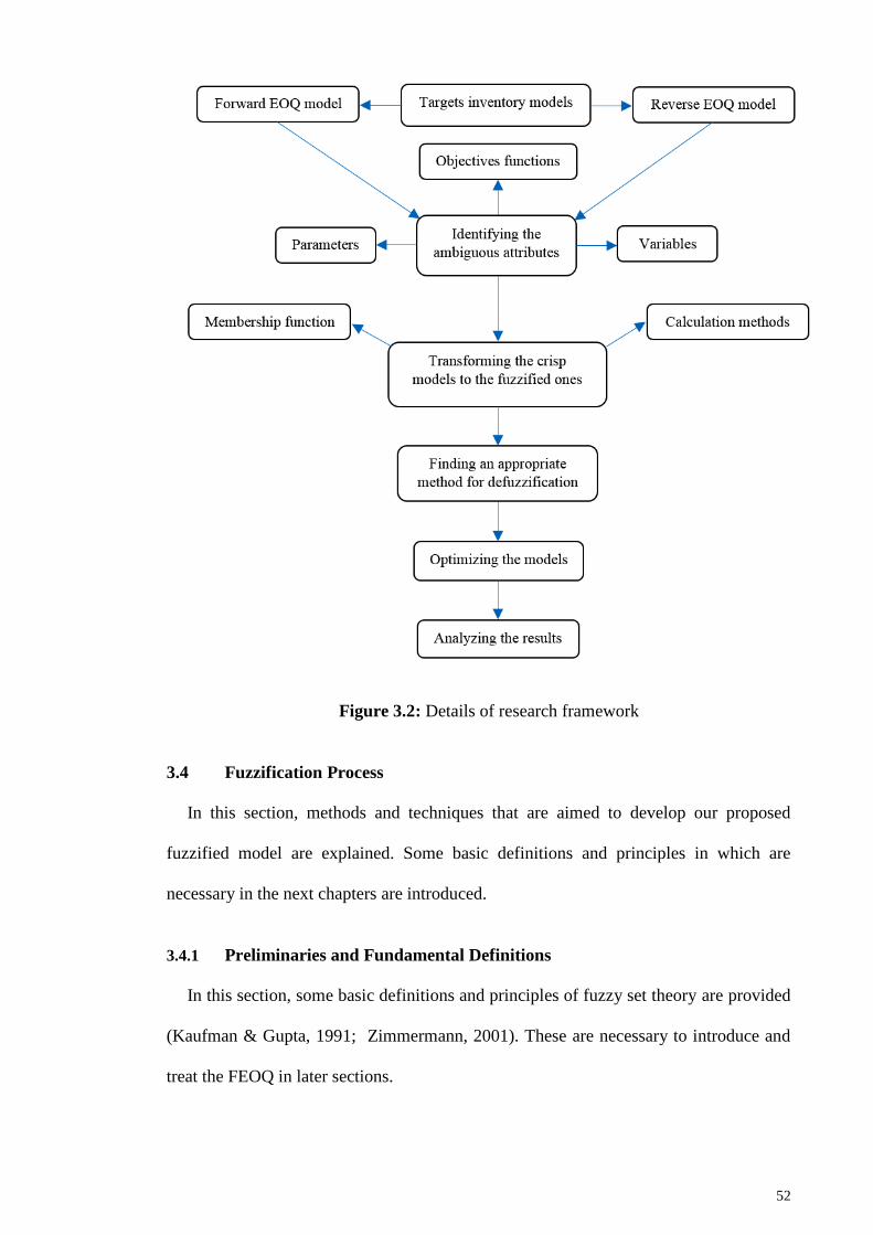
52

Figure 3.2: Details of research framework

3.4 Fuzzification Process

In this section, methods and techniques that are aimed to develop our proposed

fuzzified model are explained. Some basic definitions and principles in which are

necessary in the next chapters are introduced.

3.4.1 Preliminaries and Fundamental Definitions

In this section, some basic definitions and principles of fuzzy set theory are provided

(Kaufman & Gupta, 1991; Zimmermann, 2001). These are necessary to introduce and

treat the FEOQ in later sections.

53

Definition. 1: Let 𝑈 be a universe set. A fuzzy set Β̃ of 𝑈 is defined by a membership

function 𝜇Β̃(𝑢) → [0,1] where 𝜇Β̃(𝑢), ∀𝑢 ∈ 𝑈 denotes the grade of membership.

Definition. 2: The fuzzy subset Β̃ in the universe of discourse is called as a normal set if

and only if 𝑠𝑢𝑝𝑢∈𝑈𝜇Β̃(𝑢) = 1. That is, the largest grade that an element can obtain.

Definition. 3: A fuzzy subset Β̃ of the universe of discourse 𝑈 is convex if and only if for

all 𝑢1 and 𝑢2 ∈ 𝑈 and for 𝛾 ∈ [0,1] we have: 𝜇Β̃(𝛾𝑢1 + (1 − 𝛾)𝑢2) ≥

min(𝜇Β̃(𝑢1), 𝜇Β̃(𝑢2)).

Definition. 4: A fuzzy set Β̃ is a fuzzy number if and only if it is normal and convex on

𝑈.

Definition. 5: Fuzzy set Β̃𝛼 for 0 ≤ 𝛼 ≤ 1 and a range of 𝑢 ∈ 𝑅 is called an 𝛼-level fuzzy

point whose membership function has a form

𝜇Β̃𝛼(𝑢) = {𝛼, 𝑢 = 𝑎,0, 𝑢 ≠ 𝑎. (3.1)

It should be noted that if 𝛼 = 1, the membership function of the 1-level fuzzy point Β̃𝛼

becomes the characteristic function, i.e.,

𝜇Β̃𝛼(𝑢) = {1, 𝑢 = 𝑎,0, 𝑢 ≠ 𝑎.

(3.2)

In this case, the fuzzy point Β̃1 and the real number 𝑎 ∈ 𝑅 are similar except for their

representation.

Definition. 6: For 0 ≤ 𝛼 ≤ 1 and 𝑎 < 𝑏, the fuzzy set [𝑎𝛼, 𝑏𝛼] defined on𝑅 is called an

𝛼-level fuzzy interval if its membership function is given by

𝜇[𝑎𝛼,𝑏𝛼](𝑢) = {𝛼, 𝑎 ≤ 𝑢 ≤ 𝑏,0, otherwise.

(3.3)

54

Definition. 7: The 𝛼-cut of a fuzzy set Β̃ which is presented as Β(𝛼) on 𝑅 for 0 ≤ 𝛼 ≤ 1

includes points 𝑢 such that 𝜇Β̃(𝑢) ≥ 𝛼, that is Β(𝛼) = {𝑢|𝜇Β̃(𝑢) ≥ 𝛼}.

3.4.2 Generalized Fuzzy Numbers

Generalized fuzzy number Β̃ is described as any fuzzy subset of the real line 𝑅 with

the membership function 𝜇Β̃ which is a continuous mapping from 𝑅 to the closed interval

[0,1] satisfying the below conditions:

𝜇Β̃(𝑢) = 0, −∞ < 𝑥 ≤ 𝛽1;

𝜇Β̃(𝑢) = 𝑀(𝑢) is a strictly increasing function for 𝛽1 ≤ 𝑥 ≤ 𝛽2;

𝜇Β̃(𝑢) = 𝑤Β, 𝛽2 ≤ 𝑥 ≤ 𝛽3;

𝜇Β̃(𝑢) = 𝑁(𝑢) is a strictly decreasing function for 𝛽3 ≤ 𝑥 ≤ 𝛽4;

𝜇Β̃(𝑢) = 0, 𝛽4 ≤ 𝑥 < ∞.

where 0 < 𝑤Β ≤ 1, and 𝛽𝑖,𝑖 = 1,2,3,4 are real numbers. This type of generalized

fuzzy number could be written as Β̃ = (𝛽1, 𝛽2, 𝛽3, 𝛽4; 𝑤Β)𝑀𝑁, and it is called a trapezoidal

fuzzy number (TPFN). When 𝑤Β = 1, it easily could be shown as Β̃ = (𝛽1, 𝛽2, 𝛽3, 𝛽4)𝑀𝑁

that is a normalized fuzzy number. If 𝛽2 = 𝛽3 = 𝛽 then it is transformed to a triangular

fuzzy number (TFN) which could be presented as T̃ = (𝛽1, 𝛽, 𝛽4; 𝑤Β)𝑀𝑁 and its normal

form is shown as T̃ = (𝛽1, 𝛽, 𝛽4)𝑀𝑁. When 𝛽1 = 𝛽 = 𝛽4 = 𝛽′, then the TFN �̃� =

(𝛽′, 𝛽′, 𝛽′) is identical to the 1-level fuzzy point T̃1.

Definition. 8: For 𝛼 ∈ [0,1], the 𝛼-cut of TFN Β̃ = (𝛽1, 𝛽, 𝛽4) is Β(𝛼) = [Β𝐿(𝛼), Β𝑅(𝛼)],

where Β𝐿(𝛼) = 𝛽1 + (𝛽 − 𝛽1)𝛼 and Β𝑅(𝛼) = 𝛽4 − (𝛽4 − 𝛽)𝛼.

3.4.3 Overview of the Previous Fuzzy Numbers

Many kinds of fuzzy numbers have been used in the literature that include trapezoidal

and triangular fuzzy numbers, Gaussian fuzzy number, interval fuzzy number, statistic-

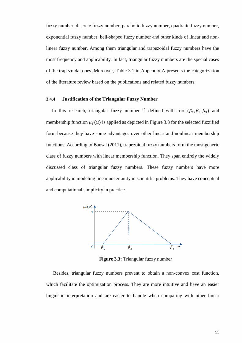
55

fuzzy number, discrete fuzzy number, parabolic fuzzy number, quadratic fuzzy number,

exponential fuzzy number, bell-shaped fuzzy number and other kinds of linear and non-

linear fuzzy number. Among them triangular and trapezoidal fuzzy numbers have the

most frequency and applicability. In fact, triangular fuzzy numbers are the special cases

of the trapezoidal ones. Moreover, Table 3.1 in Appendix A presents the categorization

of the literature review based on the publications and related fuzzy numbers.

3.4.4 Justification of the Triangular Fuzzy Number

In this research, triangular fuzzy number T̃ defined with trio (𝛽1, 𝛽2, 𝛽3) and

membership function 𝜇T̃(𝑢) is applied as depicted in Figure 3.3 for the selected fuzzified

form because they have some advantages over other linear and nonlinear membership

functions. According to Bansal (2011), trapezoidal fuzzy numbers form the most generic

class of fuzzy numbers with linear membership function. They span entirely the widely

discussed class of triangular fuzzy numbers. These fuzzy numbers have more

applicability in modeling linear uncertainty in scientific problems. They have conceptual

and computational simplicity in practice.

Figure 3.3: Triangular fuzzy number

Besides, triangular fuzzy numbers prevent to obtain a non-convex cost function,

which facilitate the optimization process. They are more intuitive and have an easier

linguistic interpretation and are easier to handle when comparing with other linear

56

membership functions. It is guaranteed to achieve computational efficiency and ease-of-

use to the problem (Shekarian et al., 2014b).

3.4.5 Overview of the Previous Fuzzification Methods

According to the investigated literature, there are different fuzzification methods that

are applied to transform the crisp model to the fuzzy environment. Depending on the

complexity of the model, these methods may vary. The methods of defuzzification of the

previous studies are categorized in Table 3.2 in Appendix B. Among these methods such

as possibility/necessity methods, extension principle, interval operations, as it is clear

function principle has been used in some studies.

3.4.6 Fuzzy Arithmetic

In order to do the calculations through the proposed fuzzified inventory models, it is

preferred to use the function principle method. In the next section, it is explained why this

method takes the priority to be applied. Here this method is explained via trapezoidal

fuzzy number. However, as the triangular fuzzy numbers are the special cases of the

trapezoidal ones, therefore, the derived formula and principle could be easily hold for

TFNs.

Chen (1985) suggested arithmetical operations of the function principle method as

follows. Consider the below relation in which shows the induction of the fuzzy number

Β̃ from a set of fuzzy numbers belonging to the same family.

𝑓𝑔(Β̃1, Β̃2, … , Β̃𝑛) = Β̃ = (Η, Θ, Ι, Κ; 𝑤Β)𝑀𝑁 (3.4)

where 𝑔 is a mapping from 𝑛 −dimensional real numbers 𝑅𝑛 into the real line 𝑅 and

equivalently 𝑓𝑔 could be mapped into a fuzzy number from 𝑛 −dimensional fuzzy

numbers, Β̃𝑖 = (휁𝑖 , 𝜆𝑖, 𝜇𝑖 , 𝜗𝑖; 𝑤i); 𝑖 = 1,2, … , 𝑛 and besides we have:

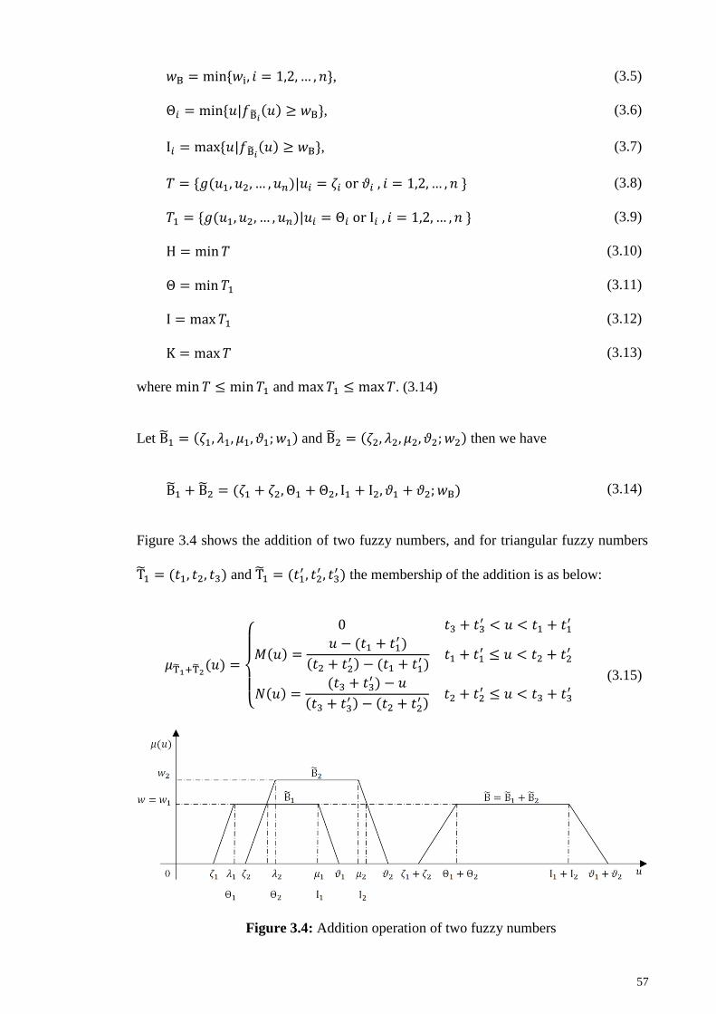
57

𝑤Β = min{𝑤i, 𝑖 = 1,2, … , 𝑛}, (3.5)

Θ𝑖 = min{𝑢|𝑓Β̃𝑖(𝑢) ≥ 𝑤Β}, (3.6)

Ι𝑖 = max{𝑢|𝑓Β̃𝑖(𝑢) ≥ 𝑤Β}, (3.7)

𝑇 = {𝑔(𝑢1, 𝑢2, … , 𝑢𝑛)|𝑢𝑖 = 휁𝑖 or𝜗𝑖, 𝑖 = 1,2, … , 𝑛} (3.8)

𝑇1 = {𝑔(𝑢1, 𝑢2, … , 𝑢𝑛)|𝑢𝑖 = Θ𝑖 orΙ𝑖 , 𝑖 = 1,2, … , 𝑛} (3.9)

Η = min𝑇 (3.10)

Θ = min𝑇1 (3.11)

Ι = max𝑇1 (3.12)

Κ = max𝑇 (3.13)

where min𝑇 ≤ min𝑇1 and max𝑇1 ≤ max𝑇. (3.14)

Let Β̃1 = (휁1, 𝜆1, 𝜇1, 𝜗1; 𝑤1) and Β̃2 = (휁2, 𝜆2, 𝜇2, 𝜗2; 𝑤2) then we have

Β̃1 + Β̃2 = (휁1 + 휁2, Θ1 + Θ2, Ι1 + Ι2, 𝜗1 + 𝜗2; 𝑤Β) (3.14)

Figure 3.4 shows the addition of two fuzzy numbers, and for triangular fuzzy numbers

T̃1 = (𝑡1, 𝑡2, 𝑡3) and T̃1 = (𝑡1′ , 𝑡2

′ , 𝑡3′ ) the membership of the addition is as below:

𝜇T̃1+T̃2(𝑢) =

{

0 𝑡3 + 𝑡3′ < 𝑢 < 𝑡1 + 𝑡1

′

𝑀(𝑢) =𝑢 − (𝑡1 + 𝑡1

′)

(𝑡2 + 𝑡2′ ) − (𝑡1 + 𝑡1

′)𝑡1 + 𝑡1

′ ≤ 𝑢 < 𝑡2 + 𝑡2′

𝑁(𝑢) =(𝑡3 + 𝑡3

′ ) − 𝑢

(𝑡3 + 𝑡3′ ) − (𝑡2 + 𝑡2

′ )𝑡2 + 𝑡2

′ ≤ 𝑢 < 𝑡3 + 𝑡3′

(3.15)

Figure 3.4: Addition operation of two fuzzy numbers

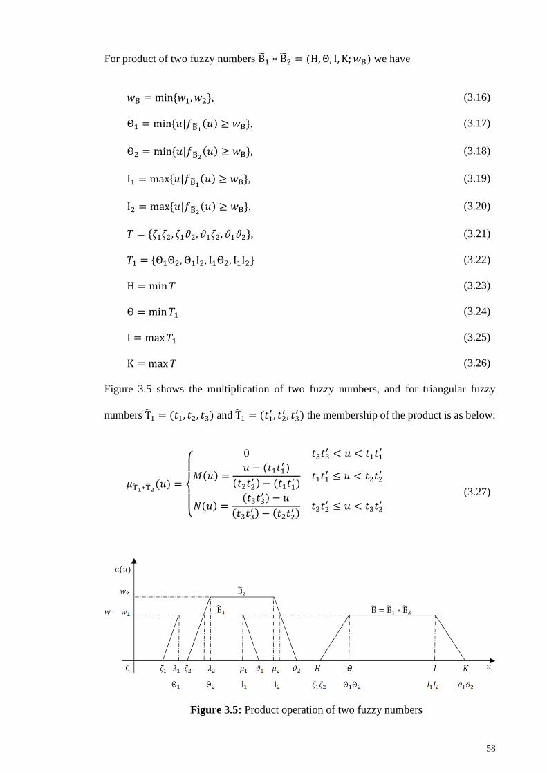
58

For product of two fuzzy numbers Β̃1 ∗ Β̃2 = (Η, Θ, Ι, Κ; 𝑤Β) we have

𝑤Β = min{𝑤1, 𝑤2}, (3.16)

Θ1 = min{𝑢|𝑓Β̃1(𝑢) ≥ 𝑤Β}, (3.17)

Θ2 = min{𝑢|𝑓Β̃2(𝑢) ≥ 𝑤Β}, (3.18)

Ι1 = max{𝑢|𝑓Β̃1(𝑢) ≥ 𝑤Β}, (3.19)

Ι2 = max{𝑢|𝑓Β̃2(𝑢) ≥ 𝑤Β}, (3.20)

𝑇 = {휁1휁2, 휁1𝜗2, 𝜗1휁2, 𝜗1𝜗2}, (3.21)

𝑇1 = {Θ1Θ2, Θ1Ι2, Ι1Θ2, Ι1Ι2} (3.22)

Η = min𝑇 (3.23)

Θ = min𝑇1 (3.24)

Ι = max𝑇1 (3.25)

Κ = max𝑇 (3.26)

Figure 3.5 shows the multiplication of two fuzzy numbers, and for triangular fuzzy

numbers T̃1 = (𝑡1, 𝑡2, 𝑡3) and T̃1 = (𝑡1′ , 𝑡2

′ , 𝑡3′ ) the membership of the product is as below:

𝜇T̃1∗T̃2(𝑢) =

{

0 𝑡3𝑡3′ < 𝑢 < 𝑡1𝑡1

′

𝑀(𝑢) =𝑢 − (𝑡1𝑡1

′)

(𝑡2𝑡2′ ) − (𝑡1𝑡1

′)𝑡1𝑡1

′ ≤ 𝑢 < 𝑡2𝑡2′

𝑁(𝑢) =(𝑡3𝑡3

′ ) − 𝑢

(𝑡3𝑡3′ ) − (𝑡2𝑡2

′ )𝑡2𝑡2

′ ≤ 𝑢 < 𝑡3𝑡3′

(3.27)

Figure 3.5: Product operation of two fuzzy numbers

59

The membership of subtraction and the division of the T̃1 = (𝑡1, 𝑡2, 𝑡3) and T̃1 =

(𝑡1′ , 𝑡2

′ , 𝑡3′ ) can be given as below:

𝜇T̃1−T̃2(𝑢) =

{

0 𝑡3 − 𝑡1′ < 𝑢 < 𝑡1 − 𝑡3

′

𝑀(𝑢) =𝑢 − (𝑡1 − 𝑡3

′ )

(𝑡2 − 𝑡2′ ) − (𝑡1 − 𝑡3

′ )𝑡1 − 𝑡3

′ ≤ 𝑢 < 𝑡2 − 𝑡2′

𝑁(𝑢) =(𝑡3 − 𝑡1

′) − 𝑢

(𝑡3 − 𝑡1′) − (𝑡2 − 𝑡2

′ )𝑡2 − 𝑡2

′ ≤ 𝑢 < 𝑡3 − 𝑡1′

(3.28)

𝜇T̃1/T̃2(𝑢) =

{

0 𝑡3/𝑡1′ < 𝑢 < 𝑡1/𝑡3

′

𝑀(𝑢) =𝑢 − (𝑡1/𝑡3

′ )

(𝑡2/𝑡2′ ) − (𝑡1/𝑡3

′ )𝑡1/𝑡3

′ ≤ 𝑢 < 𝑡2/𝑡2′

𝑁(𝑢) =(𝑡3/𝑡1

′) − 𝑢

(𝑡3/𝑡1′) − (𝑡2/𝑡2

′ )𝑡2/𝑡2

′ ≤ 𝑢 < 𝑡3/𝑡1′

(3.29)

where 𝑡1, 𝑡1′ , 𝑡2, 𝑡2

′ , 𝑡3, and 𝑡3′ are real numbers.

3.4.7 Principle of Decomposition Theory

Suppose that Β̃ is a fuzzy set on 𝑅, 0 ≤ 𝛼 ≤ 1, and its 𝛼-cut is Β(𝛼) = [Β𝐿(𝛼), Β𝑅(𝛼)]

which is a closed interval, then we have:

Β̃ = ⋃ [Β𝐿(𝛼)𝛼, Β𝑅(𝛼)𝛼]

0≤𝛼≤1

= ⋃ 𝛼Β(𝛼)

0≤𝛼≤1

(3.30)

or

𝜇Β̃(𝑢) =⋁ 𝜇[Β𝐿(𝛼)𝛼,Β𝑅(𝛼)𝛼](𝑢)

0≤𝛼≤1=⋁ 𝛼𝐶Β(𝛼)(𝑢)

0≤𝛼≤1 (3.31)

where

(𝑖) 𝛼Β(𝛼) is a fuzzy set with the membership function:

𝜇𝛼Β(𝛼)(𝑢) = {𝛼, 𝑢 ∈ Β(𝛼),0,𝑜𝑡ℎ𝑒𝑟𝑤𝑖𝑠𝑒.

(3.32)

(𝑖𝑖) 𝐶Β(𝛼)(𝑢) is a characteristic function of Β(𝛼); that is

60

𝐶Β(𝛼)(𝑢) = {1, 𝑢 ∈ Β(𝛼),0,𝑢 ∉ Β(𝛼).

(3.33)

For any 𝑎1, 𝑎2, 𝑏1, 𝑏2, 𝑘 ∈ 𝑅, 𝑎1 < 𝑎2, and 𝑏1 < 𝑏2, the interval operations are as follows:

[𝑎1, 𝑎2](+)[𝑏1, 𝑏2] = [𝑎1 + 𝑏1, 𝑎2 + 𝑏2], (3.34)

[𝑎1, 𝑎2](−)[𝑏1, 𝑏2] = [𝑎1 − 𝑏2, 𝑎2 − 𝑏1]. (3.35)

𝑘(∙)[𝑎1, 𝑎2] = {[𝑘𝑎1, 𝑘𝑎2],𝑘 > 0,[𝑘𝑎2, 𝑘𝑎1],𝑘 < 0.

(3.36)

Besides, if 0 < 𝑎1, and 0 < 𝑏1, then

[𝑎1, 𝑎2](∙)[𝑏1, 𝑏2] = [𝑎1𝑏1, 𝑎2𝑏2] (3.37)

[𝑎1, 𝑎2](÷)[𝑏1, 𝑏2] = [𝑎1𝑏2,𝑎2𝑏1]. (3.38)

3.4.8 Justification of the Function Principle Methods

As it was explained, function principle method is used to do operation of addition,

multiplication, subtract, division of triangular fuzzy numbers in present research.

Comparing with another well-known method (i.e. extension principle) which is not

simple in most of the cases, it has some advantages as follows (Shekarian et al., 2014b;

Chen & Chang, 2008):

The function principle is easier to calculate

The shape of trapezoidal and triangular fuzzy numbers does not change after

the multiplication. However, extension principle changes the shape of fuzzy

numbers to be drummed.

In contrast to the other similar methods, it can easily find the results of

multiplying more than four triangular fuzzy numbers by pointwise

computation.

61

3.5 Defuzzification Process

Although the inventory system is developed in a fuzzy environment, the results should

be transformed to the precise information to be applicable in the real situation. Because

it is not possible for the decision maker to draw ultimate conclusions with the fuzzy

results. Therefore, in order to interpret the optimal policies, it is necessary to convert the

uncertain output to the crisp ones. The method of extracting crisp results from the fuzzy

models is known as defuzzification (Mahata & Goswami, 2013). In the following,

defuzzification methods used in the literature are reviewed and techniques that are applied

in our study are explained.

3.5.1 Overview of the Previous Defuzzification Methods

In this section, defuzzification methods that are used in the previous literature are

determined according to the studies in which are gathered in chapter 2. Different direct

methods apply to the process of defuzzification such as median rule, centroid method.

Also in other models, the process applies indirectly such as reduction of fuzzy inventory

problem to a pair of mathematical programs to derive the upper bound and lower bound

or converting the problem to a chance constrained programming problem. These methods

are categorized in Table 3.3 in Appendix C. In this study, signed distance method and

GMIR method are employed to do the mentioned process.

3.5.1.1 GMIR Method

In this section, the GMIR method introduced by Chen (1985) and Chen and Hsieh

(1999) that is based on the integral value of graded mean 𝛼-level of generalized fuzzy

numbers is explained for defuzzifying them.

If 𝑀−1 and 𝑁−1 are considered as the inverse functions of 𝑀 and 𝑁 respectively in the

generalized fuzzy number Β̃ = (𝛽1, 𝛽2, 𝛽3, 𝛽4; 𝑤Β)𝑀𝑁, then the graded mean 𝛼-level value

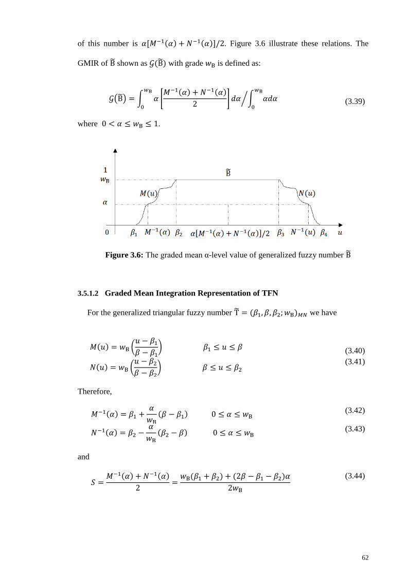
62

of this number is 𝛼[𝑀−1(𝛼) + 𝑁−1(𝛼)]/2. Figure 3.6 illustrate these relations. The

GMIR of Β̃ shown as 𝒢(Β̃) with grade 𝑤Β is defined as:

𝒢(Β̃) = ∫ 𝛼 [

𝑀−1(𝛼) + 𝑁−1(𝛼)

2] 𝑑𝛼

𝑤Β

0

∫ 𝛼𝑑𝛼𝑤Β

0

⁄

(3.39)

where 0 < 𝛼 ≤ 𝑤Β ≤ 1.

Figure 3.6: The graded mean α-level value of generalized fuzzy number Β̃

3.5.1.2 Graded Mean Integration Representation of TFN

For the generalized triangular fuzzy number T̃ = (𝛽1, 𝛽, 𝛽2; 𝑤Β)𝑀𝑁 we have

𝑀(𝑢) = 𝑤Β (

𝑢 − 𝛽1𝛽 − 𝛽1

)𝛽1 ≤ 𝑢 ≤ 𝛽

(3.40)

𝑁(𝑢) = 𝑤Β (

𝑢 − 𝛽2𝛽 − 𝛽2

) 𝛽 ≤ 𝑢 ≤ 𝛽2 (3.41)

Therefore,

𝑀−1(𝛼) = 𝛽1 +𝛼

𝑤Β(𝛽 − 𝛽1)0 ≤ 𝛼 ≤ 𝑤Β

(3.42)

𝑁−1(𝛼) = 𝛽2 −𝛼

𝑤Β(𝛽2 − 𝛽)0 ≤ 𝛼 ≤ 𝑤Β

(3.43)

and

𝑆 =

𝑀−1(𝛼) + 𝑁−1(𝛼)

2=𝑤Β(𝛽1 + 𝛽2) + (2𝛽 − 𝛽1 − 𝛽2)𝛼

2𝑤Β

(3.44)

63

Now, employing the calculated formula for the GMIR, the graded mean integration

representation of T̃ is derived as

𝒢(T̃) = ∫ 𝛼𝑆𝑑𝛼

𝑤Β

0

∫ 𝛼𝑑𝛼𝑤Β

0

⁄

=(𝛽1 + 4𝛽 + 𝛽2)

6

(3.45)

3.5.1.3 Signed Distance Method

For any 𝑎 ∈ 𝑅, the signed distance from 𝑎 to 0 is defined as 𝑑0(𝑎, 0) = 𝑎. If 𝑎 is

positive, then the distance from 𝑎 to 0 is 𝑎 = 𝑑0(𝑎, 0); if 𝑎 is negative, the distance from

𝑎 to 0 is 𝑎 = −𝑑0(𝑎, 0). This is the reason why 𝑑0(𝑎, 0) is referred as the distance from

𝑎 to 0.

Assume that Ψ be the family of all fuzzy sets Β̃ defined on 𝑅 with which the 𝛼-cut

Β(𝛼) = [Β𝐿(𝛼), Β𝑅(𝛼)] exists for every 𝛼 ∈ [0,1], and both Β𝐿(𝛼), and Β𝑅(𝛼) are

continuous functions on 0 ≤ 𝛼 ≤ 1. Then, for any Β̃ ∈ Ψ from the principle of

decomposition theory, we have

Β̃ = ⋃ [Β𝐿(𝛼)𝛼, Β𝑅(𝛼)𝛼]0≤𝛼≤1 (3.46)

The signed distance of two end points Β𝐿(𝛼), and Β𝑅(𝛼) of the 𝛼-cut of Β̃ (i.e. Β(𝛼) =

[Β𝐿(𝛼), Β𝑅(𝛼)]) to the origin 0 is 𝑑0(Β𝐿(𝛼), 0) = Β𝐿(𝛼), and 𝑑0(Β𝑅(𝛼), 0) = Β𝑅(𝛼),

respectively.

Definition. 7:

𝑑0([Β𝐿(𝛼), Β𝑅(𝛼)],0) = [𝑑0(Β𝐿(𝛼), 0)+ 𝑑0(Β𝑅(𝛼), 0)] 2⁄ = [Β𝐿(𝛼)+Β𝑅(𝛼)] 2⁄ . (3.47)

The following one-to-one mapping relationship between 𝛼-level fuzzy interval

[Β𝐿(𝛼)𝛼, Β𝑅(𝛼)𝛼], and the real interval [Β𝐿(𝛼), Β𝑅(𝛼)] can be defined, that is

[Β𝐿(𝛼)𝛼, Β𝑅(𝛼)𝛼]↔ [Β𝐿(𝛼), Β𝑅(𝛼)] (3.48)

64

Because the 1-level fuzzy point 0̃1 has a one-to-one correspondence with the real

number 0, the signed distance of [Β𝐿(𝛼)𝛼, Β𝑅(𝛼)𝛼] to 0̃1can be give as:

𝑑([Β𝐿(𝛼)𝛼, Β𝑅(𝛼)𝛼], 0̃1) = 𝑑0([Β𝐿(𝛼), Β𝑅(𝛼)], 0) =

[Β𝐿(𝛼) + Β𝑅(𝛼)] 2⁄ (3.49)

Furthermore, for Β̃ ∈ Ψ, since the above function is continuous on 0 ≤ 𝛼 ≤ 1, the

integration can be applied to obtain the mean value of the signed distance as follows:

∫ 𝑑([Β𝐿(𝛼)𝛼, Β𝑅(𝛼)𝛼], 0̃1)𝑑𝛼 =1

2∫ [Β𝐿(𝛼)+Β𝑅(𝛼)]𝑑𝛼1

0

1

0 (3.50)

Definition. 8: For Β̃ ∈ Ψ, the signed distance of Β̃ to 0̃ can be defined as:

𝑑(Β̃, 0̃1) = ∫ 𝑑([Β𝐿(𝛼)𝛼, Β𝑅(𝛼)𝛼], 0̃1)𝑑𝛼 =1

2∫ [Β𝐿(𝛼) + Β𝑅(𝛼)]𝑑𝛼1

0

1

0 (3.51)

For the TFN Β̃ = (𝑏1, 𝑏2, 𝑏3), the signed distance from Β̃ to 0̃ is given as:

𝑑(Β̃, 0̃1) = ∫ 𝑑([Β𝐿(𝛼)𝛼, Β𝑅(𝛼)𝛼], 0̃1)𝑑𝛼 =1

4(𝑏1 + 2𝑏2 + 𝑏3)

1

0 (3.52)

For two fuzzy sets Β̃, Ε̃ ∈ Ψ where Β̃ = ⋃ [Β𝐿(𝛼)𝛼, Β𝑅(𝛼)𝛼]0≤𝛼≤1 and Ε̃ =

⋃ [Ε𝐿(𝛼)𝛼, Ε𝑅(𝛼)𝛼]0≤𝛼≤1 , and 𝑘 ∈ 𝑅, we have

Β̃(+)Ε̃ = ⋃ [(Β𝐿(𝛼)+ Ε𝐿(𝛼))𝛼, (Β𝑅(𝛼)+ Ε𝑅(𝛼))𝛼]0≤𝛼≤1 , (3.53)

Β̃(−)Ε̃ = ⋃ [(Β𝐿(𝛼)− Ε𝑅(𝛼))𝛼, (Β𝑅(𝛼)− Ε𝐿(𝛼))𝛼]0≤𝛼≤1 , (3.54)

�̃�1(∙)Β̃ = {

⋃ [(𝑘Β𝐿(𝛼))𝛼, (𝑘Β𝑅(𝛼))𝛼]0≤𝛼≤1 ,𝑘 > 0,

⋃ [(𝑘Β𝑅(𝛼))𝛼, (𝑘Β𝐿(𝛼))𝛼]0≤𝛼≤1 ,𝑘 < 0,

0̃1,𝑘 = 0.

(3.55)

For two fuzzy sets Β̃, Ε̃ ∈ Ψ and 𝑘 ∈ 𝑅,

𝑑(Β̃(+)Ε̃, 0̃1) = 𝑑(Β̃, 0̃1) + 𝑑(Ε̃, 0̃1), (3.56)

𝑑(Β̃(−)Ε̃, 0̃1) = 𝑑(Β̃, 0̃1) − 𝑑(Ε̃, 0̃1), (3.57)

(3.58)

𝑑(�̃�1(∙)Β̃, 0̃1) = 𝑘𝑑(Β̃, 0̃1).

65

3.5.2 Justification of the GMIR and SD methods

In this study, the GMIR and SD methods are used as defuzzification methods in the

proposed systems. In the second suggested model, the performance of these methods is

compared.

The preference for researchers has been shifting towards the signed distance and

GMIR methods (Shekarian et al., 2014b). As the membership function does not change

under fuzzy arithmetic operations, it is possible to evaluate the defuzzified value directly

by graded mean integration method through arithmetic operations. It is more reasonable

to discuss the grade of each point of support set of fuzzy number for representing the

fuzzy number. GMIR method is effective in the sense that it grades as the degree of each

point of support set of fuzzy number and it is possible to measure the degree of similarity

between fuzzy numbers in terms of graded mean integration values (Mahata & Goswami,

2013). On the other hand, from the membership grade viewpoint, it will be efficient to

defuzzify the fuzzy number by GMIR method instead of the centroid method (Mahata &

Mahata, 2011).

Moreover, for example, as the centriod method uses the extension principle, it

concludes more complex calculations, especially, when a fuzzy parameter appears in the

denominator (e.g., Chang, 2004). Using the SD method and the GMIR method usually do

not fail to reach in closed-form solutions. However, if the function contains many

multiplicative and complex sentences, GMIR method performs better than the SD method

and resolves mathematics cumbersome.

3.6 Optimization Methods

In this section, proposed methods are explained to solve the developed fuzzy models.

However, the solvation of the models is discussed after developing the models.

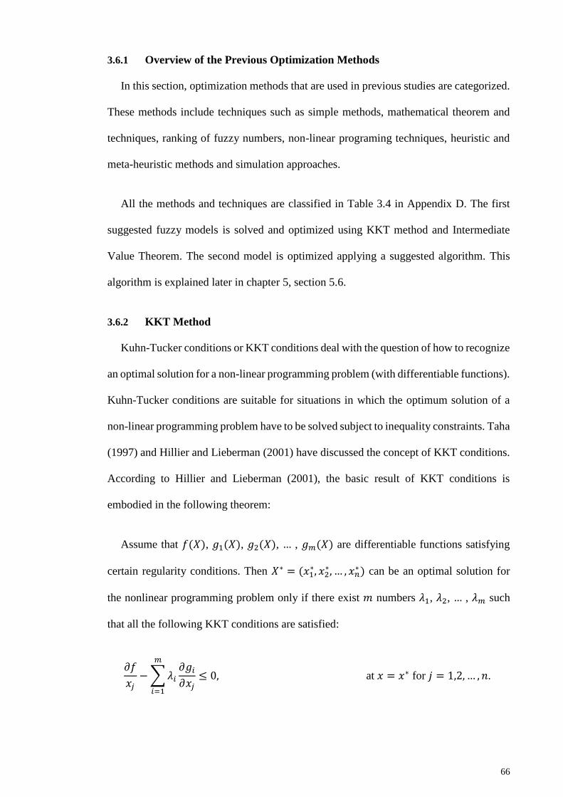
66

3.6.1 Overview of the Previous Optimization Methods

In this section, optimization methods that are used in previous studies are categorized.

These methods include techniques such as simple methods, mathematical theorem and

techniques, ranking of fuzzy numbers, non-linear programing techniques, heuristic and

meta-heuristic methods and simulation approaches.

All the methods and techniques are classified in Table 3.4 in Appendix D. The first

suggested fuzzy models is solved and optimized using KKT method and Intermediate

Value Theorem. The second model is optimized applying a suggested algorithm. This

algorithm is explained later in chapter 5, section 5.6.

3.6.2 KKT Method

Kuhn-Tucker conditions or KKT conditions deal with the question of how to recognize

an optimal solution for a non-linear programming problem (with differentiable functions).

Kuhn-Tucker conditions are suitable for situations in which the optimum solution of a

non-linear programming problem have to be solved subject to inequality constraints. Taha

(1997) and Hillier and Lieberman (2001) have discussed the concept of KKT conditions.

According to Hillier and Lieberman (2001), the basic result of KKT conditions is

embodied in the following theorem:

Assume that 𝑓(𝑋), 𝑔1(𝑋), 𝑔2(𝑋), … , 𝑔𝑚(𝑋) are differentiable functions satisfying

certain regularity conditions. Then 𝑋∗ = (𝑥1∗, 𝑥2

∗, … , 𝑥𝑛∗) can be an optimal solution for

the nonlinear programming problem only if there exist 𝑚 numbers 𝜆1, 𝜆2, … , 𝜆𝑚 such

that all the following KKT conditions are satisfied:

𝜕𝑓

𝑥𝑗−∑𝜆𝑖

𝑚

𝑖=1

𝜕𝑔𝑖𝜕𝑥𝑗

≤ 0, at 𝑥 = 𝑥∗ for 𝑗 = 1,2, … , 𝑛.

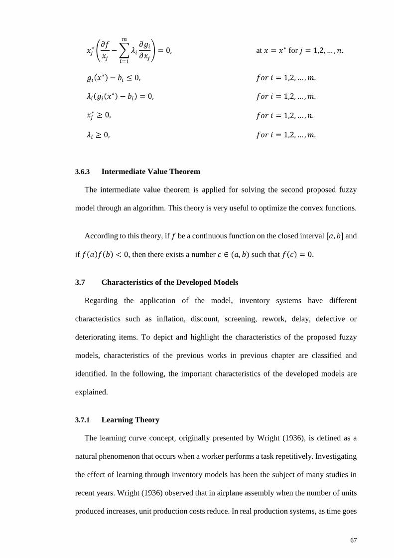
67

𝑥𝑗∗ (𝜕𝑓

𝑥𝑗−∑𝜆𝑖

𝑚

𝑖=1

𝜕𝑔𝑖𝜕𝑥𝑗

) = 0, at 𝑥 = 𝑥∗ for 𝑗 = 1,2, … , 𝑛.

𝑔𝑖(𝑥∗) − 𝑏𝑖 ≤ 0, 𝑓𝑜𝑟𝑖 = 1,2, … ,𝑚.

𝜆𝑖(𝑔𝑖(𝑥∗) − 𝑏𝑖) = 0, 𝑓𝑜𝑟𝑖 = 1,2, … ,𝑚.

𝑥𝑗∗ ≥ 0, 𝑓𝑜𝑟𝑖 = 1,2, … , 𝑛.

𝜆𝑖 ≥ 0, 𝑓𝑜𝑟𝑖 = 1,2, … ,𝑚.

3.6.3 Intermediate Value Theorem

The intermediate value theorem is applied for solving the second proposed fuzzy

model through an algorithm. This theory is very useful to optimize the convex functions.

According to this theory, if 𝑓 be a continuous function on the closed interval [𝑎, 𝑏] and

if 𝑓(𝑎)𝑓(𝑏) < 0, then there exists a number 𝑐 ∈ (𝑎, 𝑏) such that 𝑓(𝑐) = 0.

3.7 Characteristics of the Developed Models

Regarding the application of the model, inventory systems have different

characteristics such as inflation, discount, screening, rework, delay, defective or

deteriorating items. To depict and highlight the characteristics of the proposed fuzzy

models, characteristics of the previous works in previous chapter are classified and

identified. In the following, the important characteristics of the developed models are

explained.

3.7.1 Learning Theory

The learning curve concept, originally presented by Wright (1936), is defined as a

natural phenomenon that occurs when a worker performs a task repetitively. Investigating

the effect of learning through inventory models has been the subject of many studies in

recent years. Wright (1936) observed that in airplane assembly when the number of units

produced increases, unit production costs reduce. In real production systems, as time goes

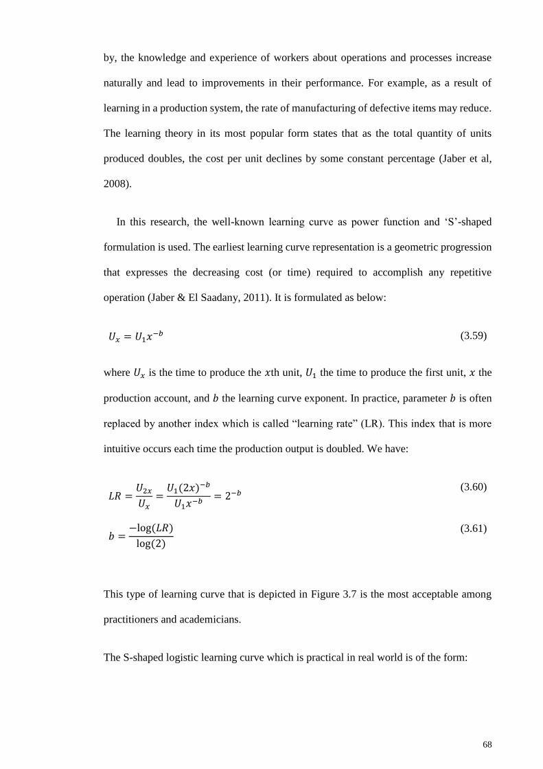
68

by, the knowledge and experience of workers about operations and processes increase

naturally and lead to improvements in their performance. For example, as a result of

learning in a production system, the rate of manufacturing of defective items may reduce.

The learning theory in its most popular form states that as the total quantity of units

produced doubles, the cost per unit declines by some constant percentage (Jaber et al,

2008).

In this research, the well-known learning curve as power function and ‘S’-shaped

formulation is used. The earliest learning curve representation is a geometric progression

that expresses the decreasing cost (or time) required to accomplish any repetitive

operation (Jaber & El Saadany, 2011). It is formulated as below:

𝑈𝑥 = 𝑈1𝑥−𝑏 (3.59)

where 𝑈𝑥 is the time to produce the 𝑥th unit, 𝑈1 the time to produce the first unit, 𝑥 the

production account, and 𝑏 the learning curve exponent. In practice, parameter 𝑏 is often

replaced by another index which is called “learning rate” (LR). This index that is more

intuitive occurs each time the production output is doubled. We have:

𝐿𝑅 =𝑈2𝑥𝑈𝑥

=𝑈1(2𝑥)

−𝑏

𝑈1𝑥−𝑏= 2−𝑏

(3.60)

𝑏 =−log(𝐿𝑅)

log(2)

(3.61)

This type of learning curve that is depicted in Figure 3.7 is the most acceptable among

practitioners and academicians.

The S-shaped logistic learning curve which is practical in real world is of the form:

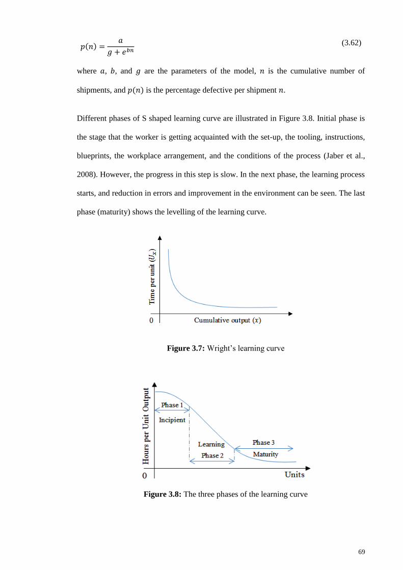
69

𝑝(𝑛) =𝑎

𝑔 + 𝑒𝑏𝑛

(3.62)

where 𝑎, 𝑏, and 𝑔 are the parameters of the model, 𝑛 is the cumulative number of

shipments, and 𝑝(𝑛) is the percentage defective per shipment 𝑛.

Different phases of S shaped learning curve are illustrated in Figure 3.8. Initial phase is

the stage that the worker is getting acquainted with the set-up, the tooling, instructions,

blueprints, the workplace arrangement, and the conditions of the process (Jaber et al.,

2008). However, the progress in this step is slow. In the next phase, the learning process

starts, and reduction in errors and improvement in the environment can be seen. The last

phase (maturity) shows the levelling of the learning curve.

Figure 3.7: Wright’s learning curve

Figure 3.8: The three phases of the learning curve

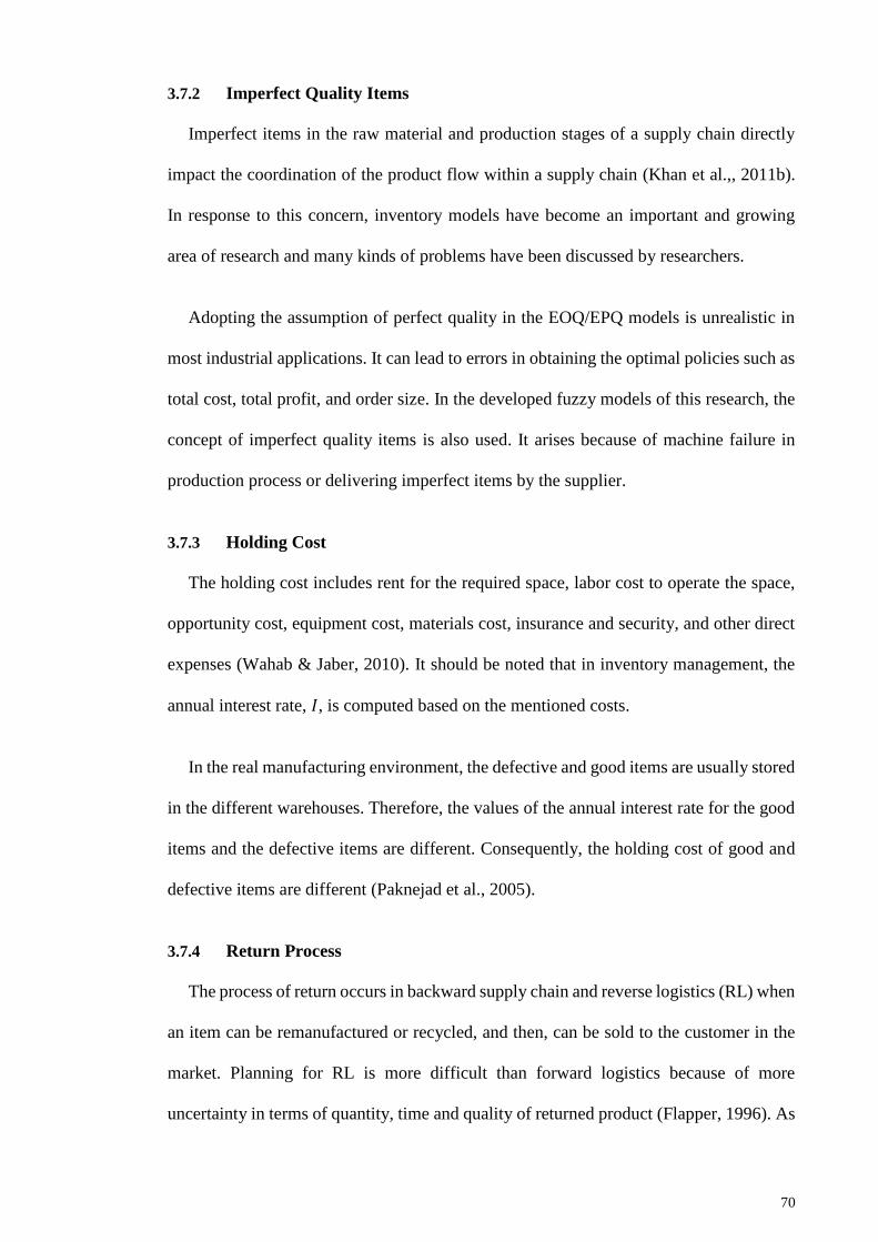
70

3.7.2 Imperfect Quality Items

Imperfect items in the raw material and production stages of a supply chain directly

impact the coordination of the product flow within a supply chain (Khan et al.,, 2011b).

In response to this concern, inventory models have become an important and growing

area of research and many kinds of problems have been discussed by researchers.

Adopting the assumption of perfect quality in the EOQ/EPQ models is unrealistic in

most industrial applications. It can lead to errors in obtaining the optimal policies such as

total cost, total profit, and order size. In the developed fuzzy models of this research, the

concept of imperfect quality items is also used. It arises because of machine failure in

production process or delivering imperfect items by the supplier.

3.7.3 Holding Cost

The holding cost includes rent for the required space, labor cost to operate the space,

opportunity cost, equipment cost, materials cost, insurance and security, and other direct

expenses (Wahab & Jaber, 2010). It should be noted that in inventory management, the

annual interest rate, 𝐼, is computed based on the mentioned costs.

In the real manufacturing environment, the defective and good items are usually stored

in the different warehouses. Therefore, the values of the annual interest rate for the good

items and the defective items are different. Consequently, the holding cost of good and

defective items are different (Paknejad et al., 2005).

3.7.4 Return Process

The process of return occurs in backward supply chain and reverse logistics (RL) when

an item can be remanufactured or recycled, and then, can be sold to the customer in the

market. Planning for RL is more difficult than forward logistics because of more

uncertainty in terms of quantity, time and quality of returned product (Flapper, 1996). As

71

it was cleared from the reviewed literature, there is a shortcoming of developing fuzzified

model in this field. In the second proposed fuzzy model, uncertainty of return rate is dealt

to fill the gap.

3.8 Chapter Summary

In this chapter, the methodology of this research was explained and illustrated by using

some flowcharts. The framework of models was demonstrated. Methods and techniques

that are necessary to develop the fuzzy models were discussed. The framework for two

proposed fuzzy models was divided in forward and backward conditions.

Fundamental concepts and related theories were explained. Methods of fuzzification,

defuzzification, and optimization were reviewed and the used ones were described. The

use of the selected methods was also justified. In later chapters, the fuzzy models will be

formulated.

72

CHAPTER 4: FULLY FUZZY FORWARD ECONOMIC ORDER QUANTITY

MODEL CONSIDERING LEARNING EFFECTS

4.1 Introduction

In this chapter, a fully fuzzy economic order quantity model in which the number of

defective items decreases under the effect of the learning process is formulated. Firstly,

the formulation of the base model is reviewed, and then, it is extended through the fuzzy

environment. The model is solved and optimized and the crisp results are compared with

fuzzy ones. In addition, the results are compared with previous works. At the end of our

discussions, some managerial insights are proposed.

4.2 Problem Description

In the following, the base problem is reviewed according to the previous studies

(Salameh & Jaber, 2000; Maddah & Jaber, 2008; Wahab & Jaber, 2010). Later, the

problem is extended from the crisp environment to the fuzzy one.

Assume a situation where a lot from the supplier is delivered to the manufacturer who

places an order with a deterministic purchasing price and ordering cost. In addition, it is

assumed that the demand of the manufacturer is a crisp value. Moreover, it is supposed

that a part of each lot that is received by the manufacturer includes percentage defectives.

The defective items are identified by a 100% screening process with a known rate. After

separation of defective items from non-defective ones, both of them are kept in different

warehouses with different holding costs. Segregation of these items helps to a better

tracking cost as it happens in many industries. These items can be kept in different

situation. It is reasonable that the holding cost of defective items is less than the holding

cost of good ones. Before shipping a new lot, good and defective items will be sold with

different selling prices such that selling price of good items is more than the defective

ones. It is assumed that the percentage of defective items decreases under the influence

73

of learning. It is a logical assumption because learning is an inherent part of the mentioned

process.

4.2.1 Assumptions

The investigated model in fuzzy environment follows the below assumptions:

i. Demand rate is constant during the planning horizon

ii. Shortages are not allowed

iii. Lead time is zero

iv. Each shipment undergoes 100% inspection process

v. Defective items are sold at a discounted price

vi. Percentage of defectives items follows a learning curve

vii. Time horizon is infinite/finite

viii. All the parameters and variables of the model are assumed to be triangular fuzzy

number

ix. It is assumed that percentage of defective items per shipment, follows the below

S-shaped logistic learning curve model:

𝑝(𝑛) =𝛼

𝛾 + 𝑒𝛽𝑛

where 𝛼, 𝛽, and 𝛾 are the parameters of the learning function.

4.2.2 Notations

The following notations are used to formulate the model:

𝐷 Demand (unit/time)

𝑦 Lot size (unit/order) (Decision variable)

𝑦𝑛 Lot size in 𝑛th shipment when learning occurs (unit/order) (Decision variable)

𝑐 Variable cost ($/unit)

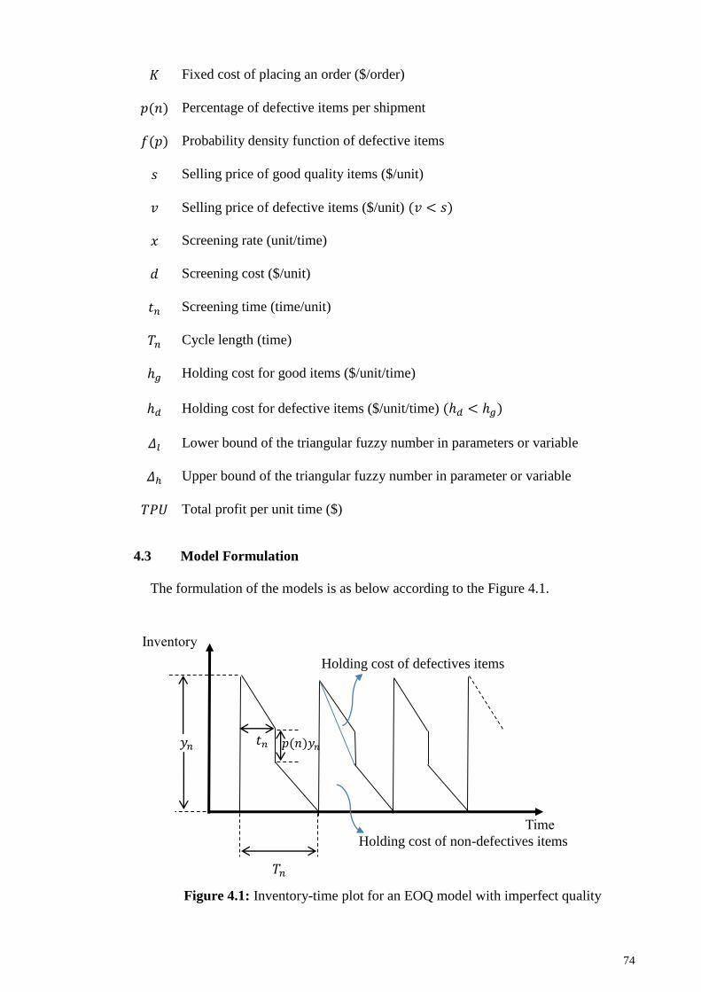
74

𝐾 Fixed cost of placing an order ($/order)

𝑝(𝑛) Percentage of defective items per shipment

𝑓(𝑝) Probability density function of defective items

𝑠 Selling price of good quality items ($/unit)

𝑣 Selling price of defective items ($/unit) (𝑣 < 𝑠)

𝑥 Screening rate (unit/time)

𝑑 Screening cost ($/unit)

𝑡𝑛 Screening time (time/unit)

𝑇𝑛 Cycle length (time)

ℎ𝑔 Holding cost for good items ($/unit/time)

ℎ𝑑 Holding cost for defective items ($/unit/time) (ℎ𝑑 < ℎ𝑔)

𝛥𝑙 Lower bound of the triangular fuzzy number in parameters or variable

𝛥ℎ Upper bound of the triangular fuzzy number in parameter or variable

𝑇𝑃𝑈 Total profit per unit time ($)

4.3 Model Formulation

The formulation of the models is as below according to the Figure 4.1.

Figure 4.1: Inventory-time plot for an EOQ model with imperfect quality

𝑝(𝑛)𝑦𝑛

𝑡𝑛

Holding cost of defectives items

Time

Inventory

𝑦𝑛

𝑇𝑛

Holding cost of non-defectives items

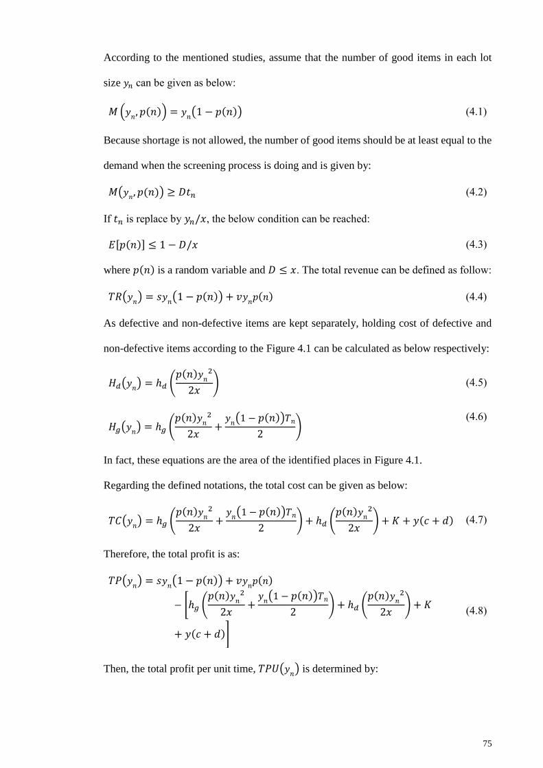
75

According to the mentioned studies, assume that the number of good items in each lot

size 𝑦𝑛 can be given as below:

𝑀(𝑦𝑛, 𝑝(𝑛)) = 𝑦

𝑛(1 − 𝑝(𝑛)) (4.1)

Because shortage is not allowed, the number of good items should be at least equal to the

demand when the screening process is doing and is given by:

𝑀(𝑦𝑛, 𝑝(𝑛)) ≥ 𝐷𝑡𝑛 (4.2)

If 𝑡𝑛 is replace by 𝑦𝑛/𝑥, the below condition can be reached:

𝐸[𝑝(𝑛)] ≤ 1 − 𝐷/𝑥 (4.3)

where 𝑝(𝑛) is a random variable and 𝐷 ≤ 𝑥. The total revenue can be defined as follow:

𝑇𝑅(𝑦𝑛) = 𝑠𝑦

𝑛(1 − 𝑝(𝑛)) + 𝑣𝑦

𝑛𝑝(𝑛) (4.4)

As defective and non-defective items are kept separately, holding cost of defective and

non-defective items according to the Figure 4.1 can be calculated as below respectively:

𝐻𝑑(𝑦𝑛) = ℎ𝑑 (𝑝(𝑛)𝑦

𝑛2

2𝑥) (4.5)

𝐻𝑔(𝑦𝑛) = ℎ𝑔 (𝑝(𝑛)𝑦

𝑛2

2𝑥+𝑦𝑛(1 − 𝑝(𝑛))𝑇𝑛

2)

(4.6)

In fact, these equations are the area of the identified places in Figure 4.1.

Regarding the defined notations, the total cost can be given as below:

𝑇𝐶(𝑦𝑛) = ℎ𝑔 (

𝑝(𝑛)𝑦𝑛2


2) + ℎ𝑑 (

𝑝(𝑛)𝑦𝑛2

2𝑥) + 𝐾 + 𝑦(𝑐 + 𝑑) (4.7)

Therefore, the total profit is as:

𝑇𝑃(𝑦𝑛) = 𝑠𝑦

𝑛(1 − 𝑝(𝑛)) + 𝑣𝑦

𝑛𝑝(𝑛)

− [ℎ𝑔 (𝑝(𝑛)𝑦

𝑛2


2) + ℎ𝑑 (

𝑝(𝑛)𝑦𝑛2

2𝑥) + 𝐾

+ 𝑦(𝑐 + 𝑑)]

(4.8)

Then, the total profit per unit time, 𝑇𝑃𝑈(𝑦𝑛) is determined by:

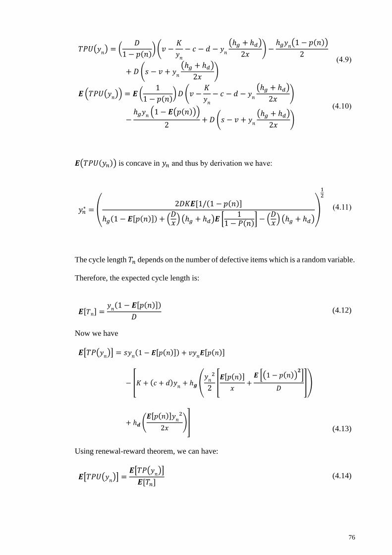
76

𝑇𝑃𝑈(𝑦𝑛) = (

𝐷

1 − 𝑝(𝑛))(𝑣 −

𝐾

𝑦𝑛

− 𝑐 − 𝑑 − 𝑦𝑛

(ℎ𝑔 + ℎ𝑑)

2𝑥) −

ℎ𝑔𝑦𝑛(1 − 𝑝(𝑛))

2

+ 𝐷 (𝑠 − 𝑣 + 𝑦𝑛

(ℎ𝑔 + ℎ𝑑)

2𝑥)

(4.9)

𝑬(𝑇𝑃𝑈(𝑦𝑛)) = 𝑬 (

1

1 − 𝑝(𝑛))𝐷 (𝑣 −

𝐾

𝑦𝑛

− 𝑐 − 𝑑 − 𝑦𝑛

(ℎ𝑔 + ℎ𝑑)

2𝑥)

−ℎ𝑔𝑦𝑛 (1 − 𝑬(𝑝(𝑛)))

2+ 𝐷 (𝑠 − 𝑣 + 𝑦

𝑛

(ℎ𝑔 + ℎ𝑑)

2𝑥)

(4.10)

𝑬(𝑇𝑃𝑈(𝑦𝑛)) is concave in 𝑦𝑛 and thus by derivation we have:

𝑦𝑛∗ = (

2𝐷𝐾𝑬[1/(1 − 𝑝(𝑛)]

ℎ𝑔(1 − 𝑬[𝑝(𝑛)]) + (𝐷𝑥) (ℎ𝑔 + ℎ𝑑)𝑬 [

11 − 𝑃(𝑛)

] − (𝐷𝑥) (ℎ𝑔 + ℎ𝑑)

)

12

(4.11)

The cycle length 𝑇𝑛 depends on the number of defective items which is a random variable.

Therefore, the expected cycle length is:

𝑬[𝑇𝑛] =𝑦𝑛(1 − 𝑬[𝑝(𝑛)])

𝐷 (4.12)

Now we have

𝑬[𝑇𝑃(𝑦𝑛)] = 𝑠𝑦

𝑛(1 − 𝑬[𝑝(𝑛)]) + 𝑣𝑦

𝑛𝑬[𝑝(𝑛)]

− [𝐾 + (𝑐 + 𝑑)𝑦𝑛+ ℎ𝒈 (

𝑦𝑛2

2[𝑬[𝑝(𝑛)]

𝑥+𝑬 [(1 − 𝑝(𝑛))

𝟐]

𝐷])

+ ℎ𝒅 (𝑬[𝑝(𝑛)]𝑦

𝑛2

2𝑥)]

(4.13)

Using renewal-reward theorem, we can have:

𝑬[𝑇𝑃𝑈(𝑦𝑛)] =

𝑬[𝑇𝑃(𝑦𝑛)]

𝑬[𝑇𝑛] (4.14)

77

𝑬[𝑇𝑃𝑈(𝑦𝑛)] =

𝐷{𝑠(1 − 𝑬[𝑝(𝑛)]) + 𝑣𝑬[𝑝(𝑛)] − 𝑐 − 𝑑}

(1 − 𝐸[𝑝(𝑛)])−

𝐾𝐷

𝑦(1 − 𝐸[𝑝(𝑛)]

−𝑦𝐷

2(1 − 𝑬[𝑝(𝑛)])[ℎ𝑔 (

𝑬[𝑝(𝑛)]

𝑥+𝑬 [(1 − 𝑝(𝑛))

2]

𝐷)

+ ℎ𝑑 (𝑬[𝑝(𝑛)]

𝑥)]

(4.15)

By derivation, we can have:

𝑦𝑛∗∗ = (

2𝐷𝐾

ℎ𝑔𝑬 [(1 − 𝑝(𝑛))2] + (

𝐷𝑥) (ℎ𝑔 + ℎ𝑑)𝑬

[𝑝(𝑛)])

12

(4.16)

If the S-shaped logistic learning function is replaced:

𝛼

𝛾 + 𝑒𝛽𝑛

in Eq. (4.9), the optimal 𝑦𝑛 in crisp situation can be obtained by derivation as below:

𝑦𝑛∗∗∗ = (

2𝐷𝐾 [1

1 − 𝑝(𝑛)]

ℎ𝑔[1 − 𝑝(𝑛)] + (𝐷𝑥) (ℎ𝑔 + ℎ𝑑) (

1[1 − 𝑝(𝑛)]

) − (𝐷𝑥) (ℎ𝑔 + ℎ𝑑)

)

12

(4.17)

4.4 Fully Fuzzy Model

In this section, the crisp model illustrated in previous section is studied in a fully fuzzy

environment by fuzzifying all the input parameters and decision variable. It is assumed

that all the model is uncertain. The uncertainty of the considered parameters and variable

are represented by the concept of the triangular fuzzy number, as explained in chapter 3.

The fuzzy parameters of the model are defined as below:

�̃� = (𝐷 − 𝛥𝑙𝐷 , 𝐷, 𝐷 + 𝛥ℎ

𝐷)

�̃� = (𝑠 − 𝛥𝑙𝑠 , 𝑠, 𝑠 + 𝛥ℎ

𝑠 )

78

�̃� = (𝑣 − 𝛥𝑙𝑣, 𝑣, 𝑣 + 𝛥ℎ

𝑣 )

ℎ̃𝑔 = (ℎ𝑔 − 𝛥𝑙ℎ𝑔 , ℎ𝑔, ℎ𝑔 + 𝛥ℎ

ℎ𝑔)

ℎ̃𝑑 = (ℎ𝑑 − 𝛥𝑙ℎ𝑑 , ℎ𝑑 , ℎ𝑑 + 𝛥ℎ

ℎ𝑑)

𝑝(n) = (𝑝(𝑛) − 𝛥𝑙𝑝(𝑛)

, 𝑝(𝑛), 𝑝(𝑛) + 𝛥ℎ𝑝(𝑛)

)

�̃� = (𝑥 − 𝛥𝑙𝑥 , 𝑥, 𝑥 + 𝛥ℎ

𝑥)

�̃� = (𝐾 − 𝛥𝑙𝐾 , 𝐾, 𝐾 + 𝛥ℎ

𝐾)

�̃� = (𝑐 − 𝛥𝑙𝑐 , 𝑐, 𝑐 + 𝛥ℎ

𝑐 )

�̃� = (𝑑 − 𝛥𝑙𝑑 , 𝑑, 𝑑 + 𝛥ℎ

𝑑)

Moreover, the decision variable is supposed to be a triangular fuzzy number and is

given by:

�̃�𝑛 = (𝑦𝑛 − 𝛥𝑙𝑦𝑛 , 𝑦𝑛, 𝑦𝑛 + 𝛥ℎ

𝑦𝑛)

Besides, we have:

𝛥𝑙𝑖 > 0 for 𝑖 = 𝐷, 𝑠, 𝑣, ℎ𝑔, ℎ𝑑, 𝑝(𝑛), 𝑥, 𝐾, 𝑐, 𝑑, 𝑦𝑛,

𝛥ℎ𝑗> 0 for 𝑗 = 𝐷, 𝑠, 𝑣, ℎ𝑔, ℎ𝑑, 𝑝(𝑛), 𝑥, 𝐾, 𝑐, 𝑑, 𝑦𝑛,

𝐷 > 𝛥𝑙𝐷 𝑠 > 𝛥𝑙

𝑠 𝑣 > 𝛥𝑙𝑣 ℎ𝑔 > 𝛥𝑙

ℎ𝑔 ℎ𝑑 > 𝛥𝑙

ℎ𝑑 𝑝(𝑛) > 𝛥𝑙𝑝(𝑛)

𝐾 > 𝛥𝑙𝐾 𝑐 > 𝛥𝑙

𝑐 𝑑 > 𝛥𝑙𝑑 𝑦𝑛 > 𝛥𝑙

𝑦𝑛 𝑥 > 𝛥𝑙𝑥

Moreover, 𝛥𝑙𝑖 and 𝛥ℎ

𝑗 are arbitrary values which can be determined through expert’s

knowledge and statistical background of the inventory data. For example, the upper bound

of the demand in its triangular fuzzy number can be considered as the highest value which

is observed for the demand in previous inventory planning horizons and, therefore, 𝛥ℎ𝐷 is

the deviation of the highest value of the demand from the most promising value. After

replacing the above triangular fuzzy numbers in the total profit per unit time formula, the

fuzzy total profit per unit time can be obtained as follows:

79

𝑇𝑃�̃�(�̃�𝑛) = �̃� (�̃� − �̃� +ℎ̃𝑔�̃�𝑛

2�̃�+ℎ̃𝑑�̃�𝑛2�̃�

)

+ (�̃�

1 − 𝑝(�̃�))(�̃� −

�̃�

�̃�𝑛− �̃� − �̃� −

ℎ̃𝑔�̃�𝑛

2�̃�−ℎ̃𝑑�̃�𝑛2�̃�

)

−ℎ̃𝑔�̃�𝑛(1 − 𝑝(�̃�))

2

(4.18)

In order to simplify the mathematical computations, the following symbols are defined:

휁 = �̃� (�̃� − �̃� +ℎ̃𝑔�̃�𝑛

2�̃�+ℎ̃𝑑�̃�𝑛2�̃�

) (4.19)

𝜉 = (�̃� −�̃�

�̃�𝑛− �̃� − �̃� −

ℎ̃𝑔�̃�𝑛

2�̃�−ℎ̃𝑑�̃�𝑛2�̃�

) (4.20)

𝜍 = (�̃�

1 − 𝑝(�̃�))

(4.21)

𝜏 =ℎ̃𝑔�̃�𝑛(1 − 𝑝(�̃�))

2

(4.22)

Since the whole parameters are triangular fuzzy numbers, each of the defined symbols

is a triangular fuzzy number. Hence, they can be considered as a triangular fuzzy number

by the following triplet components:

휁̃ = (휁1, 휁2, 휁3) (4.23)

𝜉 = (𝜉1, 𝜉2, 𝜉3) (4.24)

𝜍 = (𝜍1, 𝜍2, 𝜍3) (4.25)

𝜏 = (𝜏1, 𝜏2, 𝜏3) (4.26)

Using the function principle method described in chapter 3, the process of computations

is as below:

80

휁1 = (D − 𝛥𝑙𝐷). [[(𝑠 − 𝛥𝑙

𝑠) − (𝑣 + 𝛥ℎ𝑣)]

+(ℎ𝑔 − 𝛥𝑙

ℎ𝑔) (𝑦𝑛 − 𝛥𝑙𝑦𝑛) + (ℎ𝑑 − 𝛥𝑙

ℎ𝑑)(𝑦𝑛 − 𝛥𝑙𝑦𝑛)

2(𝑥 + 𝛥ℎ𝑥)

]

(4.27)

휁2 = 𝐷 [(𝑠 − 𝑣) +ℎ𝑔𝑦𝑛

2𝑥+ℎ𝑑𝑦𝑛2𝑥

] (4.28)

휁3 = (D + 𝛥ℎ𝐷)

. [[(𝑠 + 𝛥ℎ𝑠 ) − (𝑣 − 𝛥𝑙

𝑣)]

+(ℎ𝑔 + 𝛥ℎ

ℎ𝑔) (𝑦𝑛 + 𝛥ℎ𝑦𝑛) + (ℎ𝑑 + 𝛥ℎ

ℎ𝑑)(𝑦𝑛 + 𝛥ℎ𝑦𝑛)

2(𝑥 − 𝛥𝑙𝑥)

]

(4.29)

𝜉1 = [(𝑣 − 𝛥𝑙𝑣) −

(𝐾 + 𝛥ℎ𝐾)

(𝑦𝑛 − 𝛥𝑙𝑦𝑛)

− (𝑐 + 𝛥ℎ𝑐 ) − (𝑑 + 𝛥ℎ

𝑑)

−(ℎ𝑔 + 𝛥ℎ

ℎ𝑔) (𝑦𝑛 + 𝛥ℎ

𝑦𝑛) + (ℎ𝑑 + 𝛥ℎℎ𝑑)(𝑦𝑛 + 𝛥ℎ

𝑦𝑛)


]

(4.30)

𝜉2 = (𝑣 −𝐾

𝑦𝑛− 𝑐 − 𝑑 −

ℎ𝑔𝑦𝑛

2𝑥−ℎ𝑑𝑦𝑛2𝑥

) (4.31)

𝜉3 = [(𝑣 + 𝛥ℎ𝑣) −

(𝐾 − 𝛥𝑙𝐾)

(𝑦𝑛 + 𝛥ℎ𝑦𝑛)

− (𝑐 − 𝛥𝑙𝑐) − (𝑑 − 𝛥𝑙

𝑑)

−(ℎ𝑔 − 𝛥𝑙




]

(4.32)

𝜍1 = (𝐷 − 𝛥𝑙𝐷) [

(𝛾 + 𝛥ℎ𝛾) + 𝑒

(𝑛+𝛥ℎ𝑛)(𝛽+𝛥ℎ

𝛽)

(𝛾 + 𝛥ℎ𝛾) − (𝛼 − 𝛥𝑙

𝛼) + 𝑒(𝑛+𝛥ℎ

𝑛)(𝛽+𝛥ℎ𝛽)]

(4.33)

𝜍2 = (𝛾 + 𝑒𝑛𝛽

𝛾 + 𝑒𝑛𝛽 − 𝛼)𝐷 (4.34)

81

𝜍3 = (𝐷 + 𝛥ℎ𝐷) [

(𝛾 − 𝛥𝑙𝛾) + 𝑒

(𝑛−𝛥𝑙𝑛)(𝛽−𝛥𝑙

𝛽)

(𝛾 − 𝛥𝑙𝛾) − (𝛼 + 𝛥ℎ

𝛼) + 𝑒(𝑛−𝛥𝑙

𝑛)(𝛽−𝛥𝑙𝛽)]

(4.35)

𝜏1 = [(ℎ𝑔 − 𝛥𝑙

ℎ𝑔) (𝑦𝑛 − 𝛥𝑙𝑦𝑛)

2] [(𝛾 − 𝛥𝑙

𝛾) − (𝛼 + 𝛥ℎ


𝑛)(𝛽−𝛥𝑙𝛽)

(𝛾 − 𝛥𝑙𝛾) + 𝑒


𝛽)

]

(4.36)

𝜏2 = (ℎ𝑔𝑦𝑛

2)(𝛾 − 𝛼 + 𝑒𝑛𝛽

𝛾 + 𝑒𝑛𝛽) (4.37)

𝜏3 = [(ℎ𝑔 + 𝛥ℎ

ℎ𝑔) (𝑦𝑛 + 𝛥ℎ

𝑦𝑛)

2] [(𝛾 + 𝛥ℎ

𝛾) − (𝛼 − 𝛥𝑙


𝑛)(𝛽+𝛥ℎ𝛽)

(𝛾 + 𝛥ℎ𝛾) + 𝑒


𝛽)

]

(4.38)

Again, because all of the parameters and variable of the inventory system are triangular

fuzzy numbers, the total profit per unit time is also a triangular fuzzy number and could

be computed as below:

𝑇𝑃�̃�(�̃�𝑛) = (𝐶1, 𝐶2, 𝐶3) (4.39)

Using the defined triplet components, we have:

(𝐶1, 𝐶2, 𝐶3) = (휁1 + 𝜉1𝜍1 − 𝜏3, 휁2 + 𝜉2𝜍2 − 𝜏2, 휁3 + 𝜉3𝜍3 − 𝜏1) (4.40)

The GMIV (defuzzified value) of total profit function could be expressed as follow:

𝜑 (𝑇𝑃�̃�(�̃�𝑛)) =1

6𝐶1 +

4

6𝐶2 +

1

6𝐶3

=1

6(휁1 + 𝜉1𝜍1 − 𝜏3) +

4

6(휁2 + 𝜉2𝜍2 − 𝜏2) +

1

6(휁3 + 𝜉3𝜍3 − 𝜏1) (4.41)

By replacing the obtained terms for above symbols, it could be described as below:

82

𝜑 (𝑇𝑃�̃�(�̃�𝑛))

=1

6

(

(D − 𝛥𝑙

𝐷) [[(𝑠 − 𝛥𝑙𝑠) − (𝑣 + 𝛥ℎ

𝑣)]





]

+ (D − 𝛥𝑙𝐷) [

(𝛾 + 𝛥ℎ𝛾) + 𝑒


𝛽)

(𝛾 + 𝛥ℎ𝛾) − (𝛼 − 𝛥𝑙


𝑛)(𝛽+𝛥ℎ𝛽)] . [(𝑣 − 𝛥𝑙

𝑣) −(𝐾 + 𝛥ℎ

𝐾)

(𝑦𝑛 − 𝛥𝑙𝑦𝑛)

− (𝑐 + 𝛥ℎ𝑐 ) − (𝑑 + 𝛥ℎ

𝐷) −(ℎ𝑔 + 𝛥ℎ




]

− [(ℎ𝑔 + 𝛥ℎ

ℎ𝑔) (𝑦𝑛 + 𝛥ℎ𝑦𝑛)

2] [(𝛾 + 𝛥ℎ

𝛾) − (𝛼 − 𝛥𝑙



(𝛾 + 𝛥ℎ𝛾) + 𝑒


𝛽)

]

)

+4

6(𝐷 [(𝑠 − 𝑣) +

ℎ𝑔𝑦𝑛


]

+ 𝐷 (𝛾 + 𝑒𝑛𝛽

𝛾 + 𝑒𝑛𝛽 − 𝛼)(𝑣 −

𝐾

𝑦𝑛− 𝑐 − 𝑑 −

ℎ𝑔𝑦𝑛


)

− (ℎ𝑔𝑦𝑛

2)(𝛾 − 𝛼 + 𝑒𝑛𝛽

𝛾 + 𝑒𝑛𝛽))

+1

6

(

(𝐷 + 𝛥ℎ

𝐷) [[(𝑠 + 𝛥ℎ𝑠 ) − (𝑣 − 𝛥𝑙

𝑣)]

+(ℎ𝑔 + 𝛥ℎ




]

+ (𝐷 + 𝛥ℎ𝐷) [

(𝛾 − 𝛥𝑙𝛾) + 𝑒


𝛽)

(𝛾 − 𝛥𝑙𝛾) − (𝛼 + 𝛥ℎ


𝑛)(𝛽−𝛥𝑙𝛽)] [(𝑣 + 𝛥ℎ

𝑣 ) −(𝐾 − 𝛥𝑙

𝐾)

(𝑦𝑛 + 𝛥ℎ𝑦𝑛)

− (𝑐 − 𝛥𝑙𝑐) − (𝑑 − 𝛥𝑙

𝑑) −(ℎ𝑔 − 𝛥𝑙




]

− [(ℎ𝑔 − 𝛥𝑙

ℎ𝑔) (𝑦𝑛 − 𝛥𝑙𝑦𝑛)

2] [(𝛾 − 𝛥𝑙

𝛾) − (𝛼 + 𝛥ℎ



(𝛾 − 𝛥𝑙𝛾) + 𝑒


𝛽)

]

)

(4.42)

83

4.5 Finding Optimal Values

In this section, the model is tried to be solved using the KKT theorem described in

chapter 3. The conditions of this theory are provided and the related constraints are

constructed.

Let assume the following equations to initialize the process of finding the optimal

solution for the defuzzified inventory cost function that was obtained in previous section:

𝑦𝑛 − 𝛥𝑙𝑦𝑛 = 𝑦1 (4.43)

𝑦𝑛 = 𝑦2 (4.44)

𝑦𝑛 + 𝛥ℎ𝑦𝑛 = 𝑦3 (4.45)

The defuzzified value of the total profit function is taken as the crisp estimate of fuzzy

total profit function where it is optimized subject to the following condition:

0 < 𝑦1 ≤ 𝑦2 ≤ 𝑦3 (4.46)

Thus, the optimum solution of defuzzified total profit function can be found by

optimizing Eq. (4.42) subject to the following inequality constraints:

𝑦1 − 𝑦2 ≤ 0 (4.47)

𝑦2 − 𝑦3 ≤ 0 (4.48)

−𝑦1 < 0 (4.49)

Now the Kuhn-Tucker conditions can be employed to find the optimal solution of

defuzzified total profit function subject to the below inequalities as imposed conditions.

𝑦1 (𝜕𝑇𝑃�̃�(�̃�𝑛)

𝜕𝑦1− 𝜆1 + 𝜆3) = 0 (4.50)

84

𝑦2 (𝜕𝑇𝑃�̃�(�̃�𝑛)

𝜕𝑦2+ 𝜆1 − 𝜆2) = 0 (4.51)

𝑦3 (𝜕𝑇𝑃�̃�(�̃�𝑛)

𝜕𝑦3+ 𝜆2) = 0 (4.52)

𝑦1 − 𝑦2 ≤ 0 (4.53)

𝑦2 − 𝑦3 ≤ 0 (4.54)

−𝑦1 < 0 (4.55)

𝜆1(𝑦1 − 𝑦2) = 0 (4.56)

𝜆2(𝑦2 − 𝑦3) = 0 (4.57)

𝜆3(−𝑦1) = 0 (4.58)

𝑦1 ≥ 0, 𝑦2 ≥ 0, 𝑦3 ≥ 0 (4.59)

𝜆1 ≥ 0, 𝜆2 ≥ 0, 𝜆3 ≥ 0 (4.60)

where

𝜕𝑇𝑃�̃�(�̃�𝑛)

𝜕𝑦1=1

6[(𝐷 − 𝛥𝑙

𝐷) (𝐴 +(𝐾 + 𝛥ℎ

𝐾)

𝑦12𝐵) − 𝐴(𝐷 + 𝛥ℎ

𝐷)𝐶

−(ℎ𝑔 − 𝛥𝑙

ℎ𝑔)

2𝐶]

(4.61)

𝜕𝑇𝑃�̃�(�̃�𝑛)

𝜕𝑦2=4

6[𝐷𝐹 + (

𝐾

𝑦22− 𝐹)𝐷𝐺 −

ℎ𝑔

2𝐺]

(4.62)

𝜕𝑇𝑃�̃�(�̃�𝑛)

𝜕𝑦3=1

6[(ℎ𝑔 + 𝛥ℎ

ℎ𝑔)

2𝐵− (𝐷 − 𝛥𝑙

𝐷)𝐵𝐸

+ (𝐷 + 𝛥ℎ𝐷) (𝐸 +

(𝐾 − 𝛥𝑙𝐾)

𝑦32𝐶)]

(4.63)

The notations of the 𝐴, 𝐵, 𝐶, 𝐸, 𝐹, and 𝐺 are given as below:

85

𝐴 =(ℎ𝑔 − 𝛥𝑙

ℎ𝑔) + (ℎ𝑑 − 𝛥𝑙ℎ𝑑)


(4.64)

𝐵 =(𝛾 + 𝛥ℎ

𝛾) + 𝑒


𝛽)

(𝛾 + 𝛥ℎ𝛾) − (𝛼 − 𝛥𝑙



(4.65)

𝐶 =(𝛾 − 𝛥𝑙

𝛾) + 𝑒


𝛽)

(𝛾 − 𝛥𝑙𝛾) − (𝛼 + 𝛥ℎ



(4.66)

𝐸 =(ℎ𝑔 + 𝛥ℎ

ℎ𝑔) + (ℎ𝑑 + 𝛥ℎℎ𝑑)


(4.67)

𝐹 =ℎ𝑔 + ℎ𝑑

2𝑥

𝐺 =𝛾 + 𝑒𝑛𝛽

𝛾 + 𝑒𝑛𝛽 − 𝛼

(4.68)

(4.69)

From constraints (4.55) and (4.58), it can be deduced that 𝜆3 = 0. If 𝜆1 = 𝜆2 = 0 in

(4.56) and (4.57), then 𝑦3 < 𝑦2 < 𝑦1 and this constraint is against the constraint 0 < 𝑦1 ≤

𝑦2 ≤ 𝑦3. Therefore, 𝑦1 = 𝑦2 and 𝑦2 = 𝑦3, mean that 𝑦1 = 𝑦2 = 𝑦3 = 𝑦∗. According to

this explanation, the solution of the model can be obtained by solving Eqs. (4.50)−(4.60),

as follows:

𝜕𝑇𝑃�̃�(�̃�𝑛)

𝜕𝑦1+𝜕𝑇𝑃�̃�(�̃�𝑛)

𝜕𝑦2+𝜕𝑇𝑃�̃�(�̃�𝑛)

𝜕𝑦3= 0 (4.70)

By taking the derivations and replacing them in Eq. (4.70), the results could be given as

follow:

86

𝑦2 [𝐴(𝐷 + 𝛥ℎ𝐷)𝐶 − (𝐷 − 𝛥𝑙

𝐷)𝐴 +(ℎ𝑔 − 𝛥𝑙

ℎ𝑔)

2𝐶−(ℎ𝑔 + 𝛥ℎ

ℎ𝑔)

2𝐵+ (𝐷 − 𝛥𝑙

𝐷)𝐵𝐸

− (𝐷 + 𝛥ℎ𝐷)𝐸 − 4𝐷𝐹 + 4𝐹𝐷𝐺 + 2

ℎ𝑔

𝐺]

= (𝐷 − 𝛥𝑙𝐷)(𝐾 + 𝛥ℎ

𝐾)𝐵 + (𝐷 + 𝛥ℎ𝐷)(𝐾 − 𝛥𝑙

𝐾)𝐶 + 4𝐷𝐾𝐺

(4.71)

The solution of the Eq. (4.65) leads to the solution of the model, as follows:

𝑦 = √𝜒1𝜒2

(4.72)

where

𝜒1 = (𝐷 − 𝛥𝑙𝐷)(𝐾 + 𝛥ℎ

𝐾)𝐵 + (𝐷 + 𝛥ℎ𝐷)(𝐾 − 𝛥𝑙

𝐾)𝐶 + 4𝐾𝐷𝐺 (4.73)

𝜒2 = (𝐷 + 𝛥ℎ𝐷)(𝐴𝐶 − 𝐸) + (𝐷 − 𝛥𝑙

𝐷)(𝐵𝐸 − A) + 4𝐹𝐷(𝐺 − 1)


ℎ𝑔)

2𝐶−(ℎ𝑔 + 𝛥ℎ

ℎ𝑔)

2𝐵+ 2

ℎ𝑔

𝐺

(4.74)

4.6 Numerical Illustrations

In this section, a numerical example is presented to illustrate the application of the

suggested fuzzy model. However, the fuzzy model through a real case is discussed later.

The relevant information for this example is assumed as 𝑥 = 170,000 units per year,

𝐷 = 50,000 units per year, 𝐾 = $3,000 per order, 𝑐 = $100 per unit, 𝑠 = $200 per unit,

𝑣 = $50 per unit, 𝑑 = $0.50 per unit, ℎ𝑔 = $20 unit per year, ℎ𝑑 = $5 unit per year, 𝛾 =

819.76, 𝛼 = 70.07, and 𝛽 = 0.79. In Table 4.1, the mentioned input parameters are

fuzzified with arbitrary values. Columns 𝜑 and 𝑉 show defuzzified values and the level

of fuzziness (the percentage of difference between crisp and defuzzified values) of the

related parameters, respectively. The GMIV method is applied for defuzzification of

arbitrary levels of fuzziness.

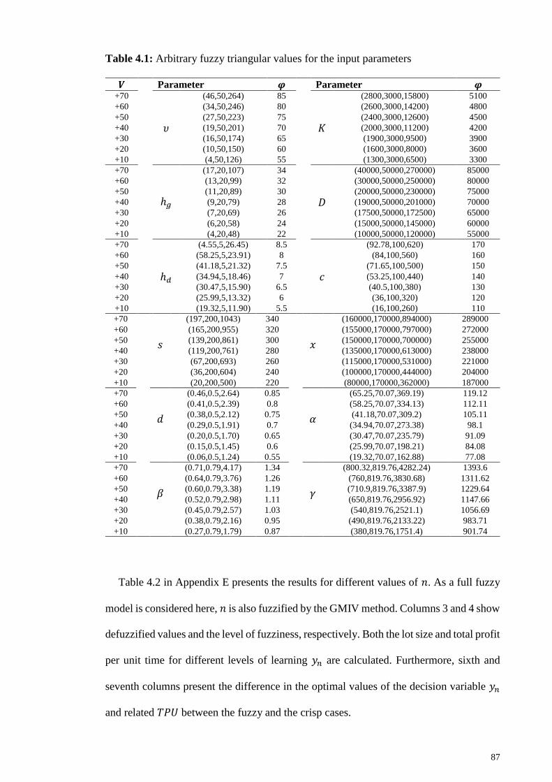
87

Table 4.1: Arbitrary fuzzy triangular values for the input parameters

𝑽 Parameter 𝝋 Parameter 𝝋 +70

𝜐

(46,50,264) 85

𝐾

(2800,3000,15800) 5100

+60 (34,50,246) 80 (2600,3000,14200) 4800

+50 (27,50,223) 75 (2400,3000,12600) 4500

+40 (19,50,201) 70 (2000,3000,11200) 4200

+30 (16,50,174) 65 (1900,3000,9500) 3900

+20 (10,50,150) 60 (1600,3000,8000) 3600

+10 (4,50,126) 55 (1300,3000,6500) 3300

+70

ℎ𝑔

(17,20,107) 34

𝐷

(40000,50000,270000) 85000

+60 (13,20,99) 32 (30000,50000,250000) 80000

+50 (11,20,89) 30 (20000,50000,230000) 75000

+40 (9,20,79) 28 (19000,50000,201000) 70000

+30 (7,20,69) 26 (17500,50000,172500) 65000

+20 (6,20,58) 24 (15000,50000,145000) 60000

+10 (4,20,48) 22 (10000,50000,120000) 55000

+70

ℎ𝑑

(4.55,5,26.45) 8.5

𝑐

(92.78,100,620) 170

+60 (58.25,5,23.91) 8 (84,100,560) 160

+50 (41.18,5,21.32) 7.5 (71.65,100,500) 150

+40 (34.94,5,18.46) 7 (53.25,100,440) 140

+30 (30.47,5,15.90) 6.5 (40.5,100,380) 130

+20 (25.99,5,13.32) 6 (36,100,320) 120

+10 (19.32,5,11.90) 5.5 (16,100,260) 110

+70

𝑠

(197,200,1043) 340

𝑥

(160000,170000,894000) 289000

+60 (165,200,955) 320 (155000,170000,797000) 272000

+50 (139,200,861) 300 (150000,170000,700000) 255000

+40 (119,200,761) 280 (135000,170000,613000) 238000

+30 (67,200,693) 260 (115000,170000,531000) 221000

+20 (36,200,604) 240 (100000,170000,444000) 204000

+10 (20,200,500) 220 (80000,170000,362000) 187000

+70

𝑑

(0.46,0.5,2.64) 0.85

𝛼

(65.25,70.07,369.19) 119.12

+60 (0.41,0.5,2.39) 0.8 (58.25,70.07,334.13) 112.11

+50 (0.38,0.5,2.12) 0.75 (41.18,70.07,309.2) 105.11

+40 (0.29,0.5,1.91) 0.7 (34.94,70.07,273.38) 98.1

+30 (0.20,0.5,1.70) 0.65 (30.47,70.07,235.79) 91.09

+20 (0.15,0.5,1.45) 0.6 (25.99,70.07,198.21) 84.08

+10 (0.06,0.5,1.24) 0.55 (19.32,70.07,162.88) 77.08

+70

𝛽

(0.71,0.79,4.17) 1.34

𝛾

(800.32,819.76,4282.24) 1393.6

+60 (0.64,0.79,3.76) 1.26 (760,819.76,3830.68) 1311.62

+50 (0.60,0.79,3.38) 1.19 (710.9,819.76,3387.9) 1229.64

+40 (0.52,0.79,2.98) 1.11 (650,819.76,2956.92) 1147.66

+30 (0.45,0.79,2.57) 1.03 (540,819.76,2521.1) 1056.69

+20 (0.38,0.79,2.16) 0.95 (490,819.76,2133.22) 983.71

+10 (0.27,0.79,1.79) 0.87 (380,819.76,1751.4) 901.74

Table 4.2 in Appendix E presents the results for different values of 𝑛. As a full fuzzy

model is considered here, 𝑛 is also fuzzified by the GMIV method. Columns 3 and 4 show

defuzzified values and the level of fuzziness, respectively. Both the lot size and total profit

per unit time for different levels of learning 𝑦𝑛 are calculated. Furthermore, sixth and

seventh columns present the difference in the optimal values of the decision variable 𝑦𝑛

and related 𝑇𝑃𝑈 between the fuzzy and the crisp cases.

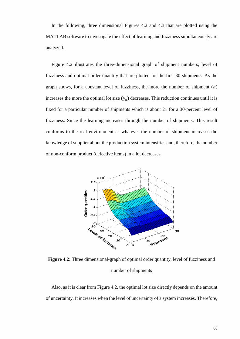
88

In the following, three dimensional Figures 4.2 and 4.3 that are plotted using the

MATLAB software to investigate the effect of learning and fuzziness simultaneously are

analyzed.

Figure 4.2 illustrates the three-dimensional graph of shipment numbers, level of

fuzziness and optimal order quantity that are plotted for the first 30 shipments. As the

graph shows, for a constant level of fuzziness, the more the number of shipment (𝑛)

increases the more the optimal lot size (𝑦𝑛) decreases. This reduction continues until it is

fixed for a particular number of shipments which is about 21 for a 30-percent level of

fuzziness. Since the learning increases through the number of shipments. This result

conforms to the real environment as whatever the number of shipment increases the

knowledge of supplier about the production system intensifies and, therefore, the number

of non-conform product (defective items) in a lot decreases.

Figure 4.2: Three dimensional-graph of optimal order quantity, level of fuzziness and

number of shipments

Also, as it is clear from Figure 4.2, the optimal lot size directly depends on the amount

of uncertainty. It increases when the level of uncertainty of a system increases. Therefore,

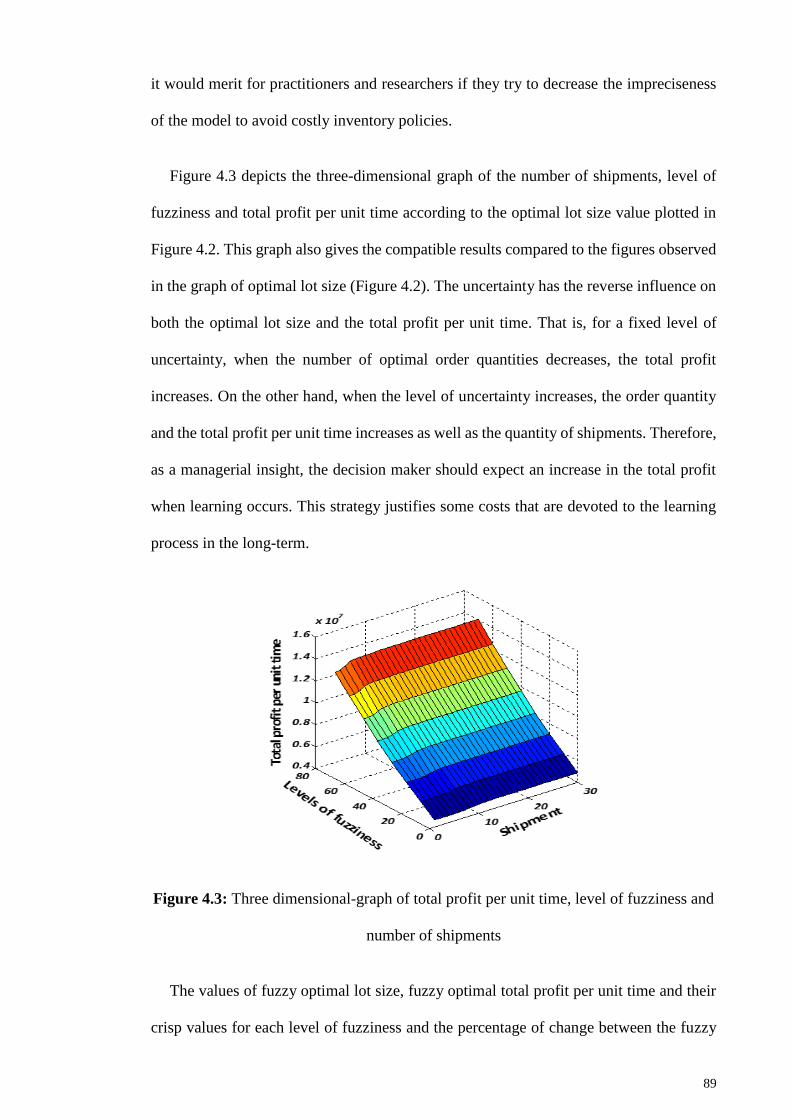
89

it would merit for practitioners and researchers if they try to decrease the impreciseness

of the model to avoid costly inventory policies.

Figure 4.3 depicts the three-dimensional graph of the number of shipments, level of

fuzziness and total profit per unit time according to the optimal lot size value plotted in

Figure 4.2. This graph also gives the compatible results compared to the figures observed

in the graph of optimal lot size (Figure 4.2). The uncertainty has the reverse influence on

both the optimal lot size and the total profit per unit time. That is, for a fixed level of

uncertainty, when the number of optimal order quantities decreases, the total profit

increases. On the other hand, when the level of uncertainty increases, the order quantity

and the total profit per unit time increases as well as the quantity of shipments. Therefore,

as a managerial insight, the decision maker should expect an increase in the total profit

when learning occurs. This strategy justifies some costs that are devoted to the learning

process in the long-term.

Figure 4.3: Three dimensional-graph of total profit per unit time, level of fuzziness and

number of shipments

The values of fuzzy optimal lot size, fuzzy optimal total profit per unit time and their

crisp values for each level of fuzziness and the percentage of change between the fuzzy

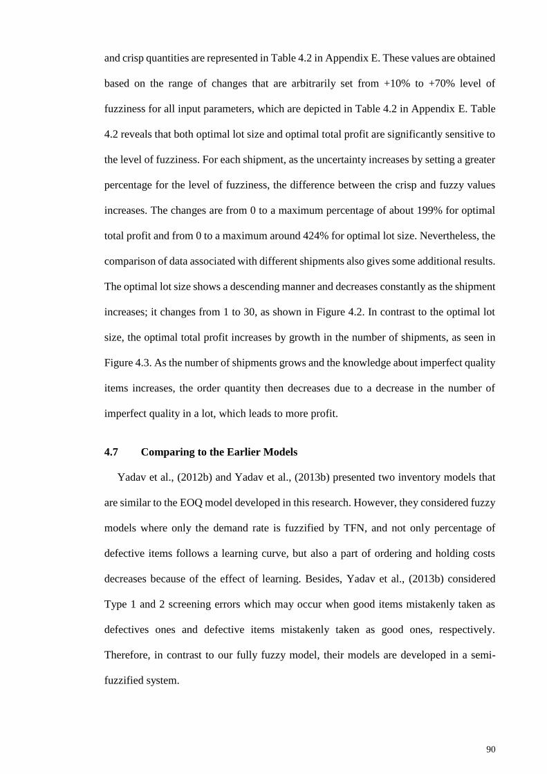
90

and crisp quantities are represented in Table 4.2 in Appendix E. These values are obtained

based on the range of changes that are arbitrarily set from +10% to +70% level of

fuzziness for all input parameters, which are depicted in Table 4.2 in Appendix E. Table

4.2 reveals that both optimal lot size and optimal total profit are significantly sensitive to

the level of fuzziness. For each shipment, as the uncertainty increases by setting a greater

percentage for the level of fuzziness, the difference between the crisp and fuzzy values

increases. The changes are from 0 to a maximum percentage of about 199% for optimal

total profit and from 0 to a maximum around 424% for optimal lot size. Nevertheless, the

comparison of data associated with different shipments also gives some additional results.

The optimal lot size shows a descending manner and decreases constantly as the shipment

increases; it changes from 1 to 30, as shown in Figure 4.2. In contrast to the optimal lot

size, the optimal total profit increases by growth in the number of shipments, as seen in

Figure 4.3. As the number of shipments grows and the knowledge about imperfect quality

items increases, the order quantity then decreases due to a decrease in the number of

imperfect quality in a lot, which leads to more profit.

4.7 Comparing to the Earlier Models

Yadav et al., (2012b) and Yadav et al., (2013b) presented two inventory models that

are similar to the EOQ model developed in this research. However, they considered fuzzy

models where only the demand rate is fuzzified by TFN, and not only percentage of

defective items follows a learning curve, but also a part of ordering and holding costs

decreases because of the effect of learning. Besides, Yadav et al., (2013b) considered

Type 1 and 2 screening errors which may occur when good items mistakenly taken as

defectives ones and defective items mistakenly taken as good ones, respectively.

Therefore, in contrast to our fully fuzzy model, their models are developed in a semi-

fuzzified system.

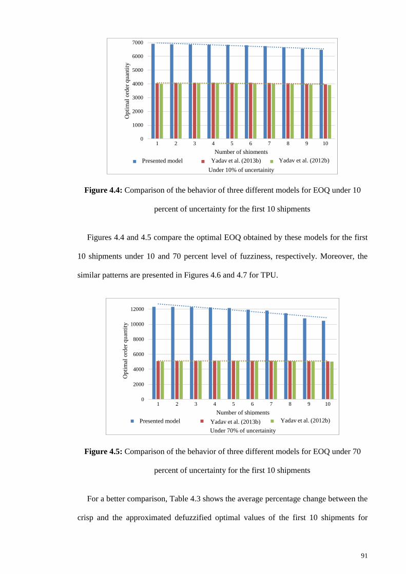
91


percent of uncertainty for the first 10 shipments

Figures 4.4 and 4.5 compare the optimal EOQ obtained by these models for the first

10 shipments under 10 and 70 percent level of fuzziness, respectively. Moreover, the

similar patterns are presented in Figures 4.6 and 4.7 for TPU.



For a better comparison, Table 4.3 shows the average percentage change between the

crisp and the approximated defuzzified optimal values of the first 10 shipments for

0

1000

2000

3000

4000

5000

6000

7000

1 2 3 4 5 6 7 8 9 10

Op

tim

al o

rder

qu

anti

ty

Number of shipments

Under 10% of uncertainity

Presented model Yadav et al. [52] Yadav et al. [53]

0

2000

4000

6000

8000

10000

12000

1 2 3 4 5 6 7 8 9 10

Op

tim

al o

rder

qu

anti

ty

Number of shipments



Yadav et al. (2012b) Yadav et al. (2013b)

Yadav et al. (2012b) Yadav et al. (2013b) Presented model

Presented model

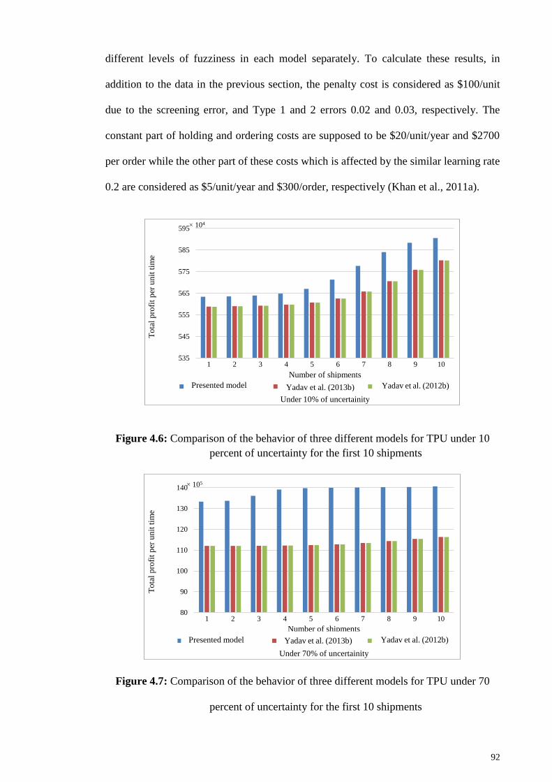
92

different levels of fuzziness in each model separately. To calculate these results, in

addition to the data in the previous section, the penalty cost is considered as $100/unit

due to the screening error, and Type 1 and 2 errors 0.02 and 0.03, respectively. The

constant part of holding and ordering costs are supposed to be $20/unit/year and $2700

per order while the other part of these costs which is affected by the similar learning rate

0.2 are considered as $5/unit/year and $300/order, respectively (Khan et al., 2011a).





535

545

555

565

575

585

595

1 2 3 4 5 6 7 8 9 10

To

tal

pro

fit

per

un

it t

ime

× 104

Number of shipments



80

90

100

110

120

130

140

1 2 3 4 5 6 7 8 9 10

To

tal

pro

fit

per

un

it t

ime

× 105

Number of shipments





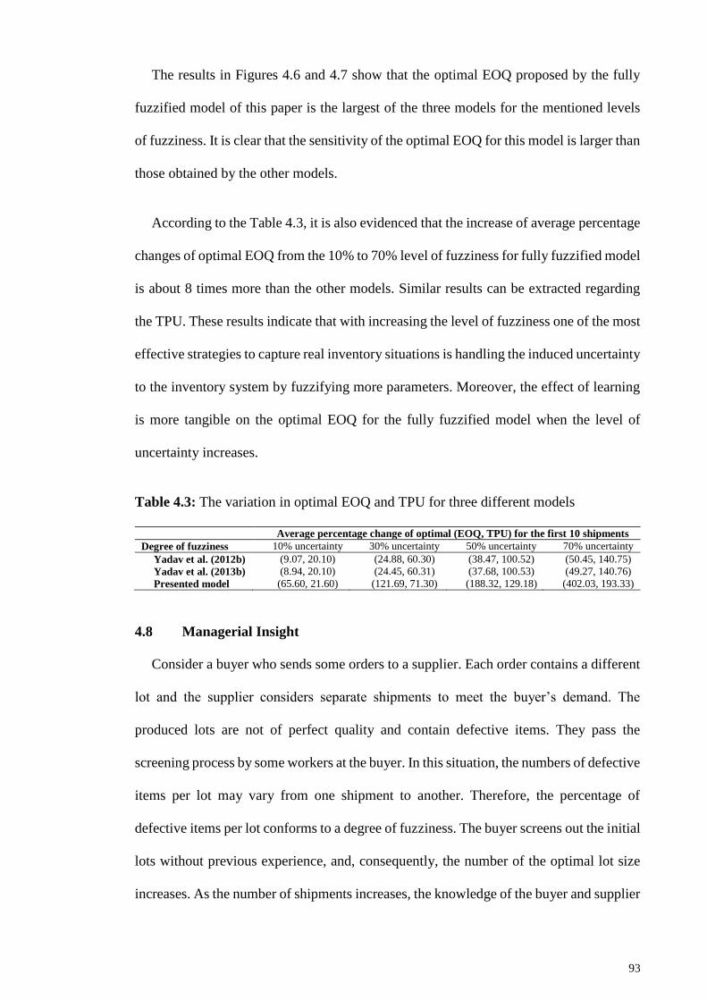
93

The results in Figures 4.6 and 4.7 show that the optimal EOQ proposed by the fully

fuzzified model of this paper is the largest of the three models for the mentioned levels

of fuzziness. It is clear that the sensitivity of the optimal EOQ for this model is larger than

those obtained by the other models.

According to the Table 4.3, it is also evidenced that the increase of average percentage

changes of optimal EOQ from the 10% to 70% level of fuzziness for fully fuzzified model

is about 8 times more than the other models. Similar results can be extracted regarding

the TPU. These results indicate that with increasing the level of fuzziness one of the most

effective strategies to capture real inventory situations is handling the induced uncertainty

to the inventory system by fuzzifying more parameters. Moreover, the effect of learning

is more tangible on the optimal EOQ for the fully fuzzified model when the level of

uncertainty increases.

Table 4.3: The variation in optimal EOQ and TPU for three different models

Average percentage change of optimal (EOQ, TPU) for the first 10 shipments

Degree of fuzziness 10% uncertainty 30% uncertainty 50% uncertainty 70% uncertainty

Yadav et al. (2012b) (9.07, 20.10) (24.88, 60.30) (38.47, 100.52) (50.45, 140.75)

Yadav et al. (2013b) (8.94, 20.10) (24.45, 60.31) (37.68, 100.53) (49.27, 140.76)

Presented model (65.60, 21.60) (121.69, 71.30) (188.32, 129.18) (402.03, 193.33)

4.8 Managerial Insight

Consider a buyer who sends some orders to a supplier. Each order contains a different

lot and the supplier considers separate shipments to meet the buyer’s demand. The

produced lots are not of perfect quality and contain defective items. They pass the

screening process by some workers at the buyer. In this situation, the numbers of defective

items per lot may vary from one shipment to another. Therefore, the percentage of

defective items per lot conforms to a degree of fuzziness. The buyer screens out the initial

lots without previous experience, and, consequently, the number of the optimal lot size

increases. As the number of shipments increases, the knowledge of the buyer and supplier

94

about the product quality preferences and production system intensifies. In the later

shipments, the buyer could transfer the information about the quality aspects of the

received product to the supplier and the supplier could modify their process or adopt some

corrective actions, and, simultaneously, the learning process will occur. Therefore,

although the number of defective items has an imprecise percentage, it could be reduced

by a close collaboration between the buyer and the supplier in gathering and processing

quality data.

For example, in foundry industries, the buyer may find some cavity problems in the

casting parts and report this quality problem to the supplier, and, consequently, the

supplier may add an X-ray operation to its production system in order to detect the cavity

in the parts before sending the parts to the buyer. Adding this operation definitely

decreases the number of defective items in future shipments. In this scenario, the decision-

makers could order smaller batches so that the number of defective items in each batch

decreases, and, consequently, they could acquire more profit.

The findings of this research give some insights to managers when they should make

a decision. When they face a great deal of uncertainty, adopting inventory policy should

be the same as when the available data are exact and accurate. They could raise the gained

profit by raising the number of the orders when uncertainty is at a high level. Through

this, they could ensure that the number of items, which does not conform with the quality,

declines using the learning process, while still meeting the financial target.

4.9 Chapter Summary

Most of the decision makers (DMs) are faced with some kind of uncertainty in making

decision as little data are available for making an appropriate decision. To deal with such

a situation, the DM has to utilize proper tools to gain reasonable and reliable insights. The

95

FST has been recognized as the most powerful tool to cope with uncertainty in situations

which the DM has less data for making good decisions.

In this chapter, an EOQ model with imperfect quality items under varying holding cost

and learning in inspection is reconsidered in a fully fuzzy situation. By applying fuzzy

arithmetic operations for obtaining fuzzy total profit function, the GMIV of fuzzy number

for defuzzifying fuzzy total profit function and Kuhn Tucker conditions, the optimal order

quantity is determined in a fuzzy situation.

The given numerical example showed that both optimal lot size and total profit are

highly sensitive to the amount of fuzziness so that they change up to two and four times,

respectively. Therefore, managers should notice that removing uncertainties form

calculations would lead to a wrong decision that may impose a lot of cost on an inventory

system. Moreover, the results reveal that optimal lot size has a descending order and

declines continuously as the shipment increases while optimal total profit increases by

growth in the number of shipment. These occur because of the learning in the system.

96

CHAPTER 5: FUZZY BACKWARD ECONOMIC ORDER/PRODUCTION

QUANTITY MODEL WITH LEARNING

5.1 Introduction

In this chapter, a fuzzy reverse inventory model that some important factors are

assumed to be imprecise is developed. The performance of two defuzzification methods

is compared to transform the model to the fuzzy environment. An algorithm is suggested

to solve the defuzzified models. The results are explained and discussed through a

comprehensive numerical example.

The rest of this chapter is organized as follows: after explaining the problem, the crisp

status of the model is overviewed. In Section 5.4, the fuzzy reverse inventory model is

developed. The solution and optimization procedures are discussed in Sections 5.5 and

5.6 respectively. Section 5.7 is related to the numerical example. Finally, the chapter is

concluded in the last section.

5.2 Problem Description

Consider a supplier or manufacturer who is supplying or producing a product that is

recyclable. In this situation, a part of the product can be returned back by the customers

to the supplier or manufacturer. In fact, it is assumed that the demand of the market is

satisfying by recovered products and newly purchased/produced products

simultaneously. Besides, it is assumed that the process follows a multi-order policy for

new products and a single setup for recovery process. Moreover, it is supposed that unit

production time of the recovered products decreases because of the effect of the learning

process.

Figure 5.1 depicts the mentioned processes. The aim is to minimize the fuzzy total cost

and obtain the recovery lot size and the number of orders for new products in an uncertain

environment.

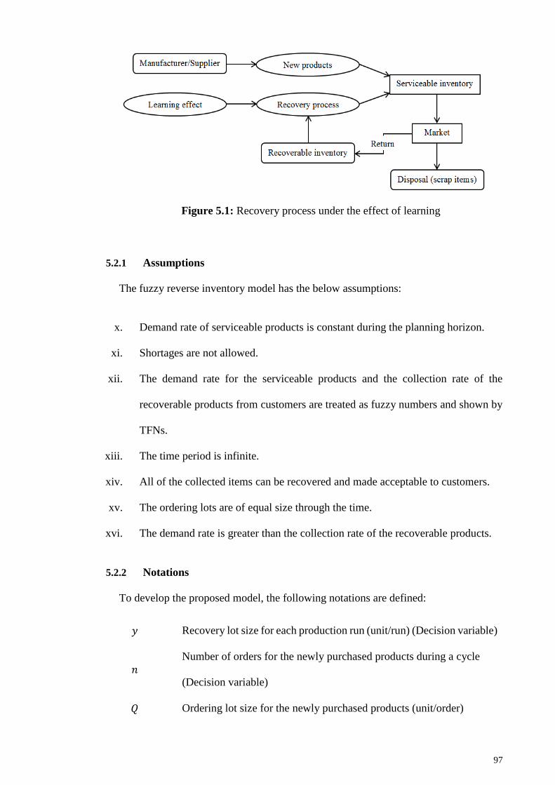
97

Figure 5.1: Recovery process under the effect of learning

5.2.1 Assumptions

The fuzzy reverse inventory model has the below assumptions:

x. Demand rate of serviceable products is constant during the planning horizon.

xi. Shortages are not allowed.

xii. The demand rate for the serviceable products and the collection rate of the

recoverable products from customers are treated as fuzzy numbers and shown by

TFNs.

xiii. The time period is infinite.

xiv. All of the collected items can be recovered and made acceptable to customers.

xv. The ordering lots are of equal size through the time.

xvi. The demand rate is greater than the collection rate of the recoverable products.

5.2.2 Notations

To develop the proposed model, the following notations are defined:

𝑦 Recovery lot size for each production run (unit/run) (Decision variable)

𝑛

Number of orders for the newly purchased products during a cycle

(Decision variable)

𝑄 Ordering lot size for the newly purchased products (unit/order)

98

𝑘

Demand rate of the serviceable products (unit/time)

(Fuzzified parameter)

𝑟

Collection rate of the recoverable products from customers (unit/time)

(Fuzzified parameter)

𝐶𝑠 Setup cost for the recovery process ($/setup)

𝐶𝑜 Ordering cost for the newly purchased products ($/order)

𝐻𝑟 Inventory holding cost for the collected products ($/unit/time)

𝐻𝑠 Inventory holding cost for the serviceable products ($/unit/time)

𝐿𝑟 Learning rate in recovery production

𝑏 Learning exponent

𝐶𝑙 Labor production cost per unit time ($/time)

𝐶𝑝 Unit purchase cost for the newly purchased products ($/unit)

𝐶𝑏 Unit buyback cost for the recovered products ($/unit)

𝑇𝐶𝑈(𝑦, 𝑛) Total cost function per unit time ($)

�̃�(𝑦, 𝑛) Fuzzified total cost function per unit time ($)

5.3 Reverse Model Formulation

Ordering cost for new items and production setup cost can be calculated as below:

𝑛𝐶𝑜 + 𝐶𝑠 (5.1)

The holding cost for the collected products can be computed according to the Figure

5.2 where 𝑇1, 𝑇2, and 𝑇 are time of the recovery process, production time of the recovery

process, and cycle length of the model respectively. Besides, 𝑅 is inventory level of the

collected products to start the recovery process. It is assumed that time required to recover

the 𝑥th unit of returned item follows the Wright learning curve explained in chapter 3 as

below:

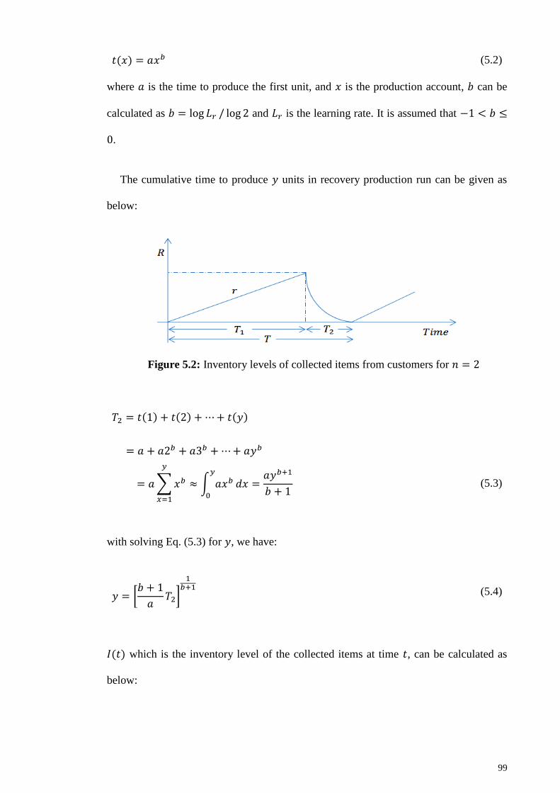
99

𝑡(𝑥) = 𝑎𝑥𝑏 (5.2)

where 𝑎 is the time to produce the first unit, and 𝑥 is the production account, 𝑏 can be

calculated as 𝑏 = log 𝐿𝑟 / log 2 and 𝐿𝑟 is the learning rate. It is assumed that −1 < 𝑏 ≤

0.

The cumulative time to produce 𝑦 units in recovery production run can be given as

below:

Figure 5.2: Inventory levels of collected items from customers for 𝑛 = 2

𝑇2 = 𝑡(1) + 𝑡(2) + ⋯+ 𝑡(𝑦)

= 𝑎 + 𝑎2𝑏 + 𝑎3𝑏 +⋯+ 𝑎𝑦𝑏

= 𝑎∑𝑥𝑏𝑦

𝑥=1

≈ ∫ 𝑎𝑥𝑏𝑦

0

𝑑𝑥 =𝑎𝑦𝑏+1

𝑏 + 1 (5.3)

with solving Eq. (5.3) for 𝑦, we have:

𝑦 = [𝑏 + 1

𝑎𝑇2]

1𝑏+1

(5.4)

𝐼(𝑡) which is the inventory level of the collected items at time 𝑡, can be calculated as

below:

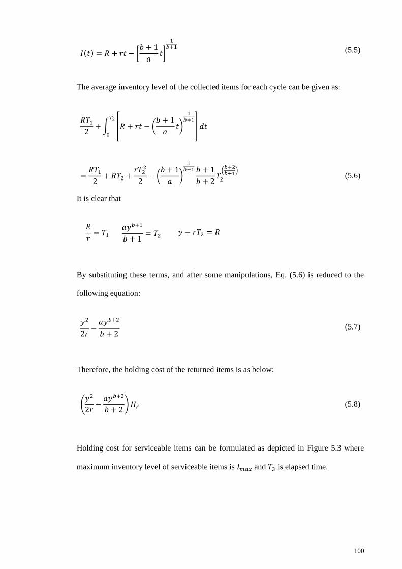
100

𝐼(𝑡) = 𝑅 + 𝑟𝑡 − [𝑏 + 1

𝑎𝑡]

1𝑏+1

(5.5)

The average inventory level of the collected items for each cycle can be given as:

𝑅𝑇12+∫ [𝑅 + 𝑟𝑡 − (

𝑏 + 1

𝑎𝑡)

1𝑏+1

] 𝑑𝑡𝑇2

0

=𝑅𝑇12+ 𝑅𝑇2 +

𝑟𝑇22

2− (

𝑏 + 1

𝑎)

1𝑏+1 𝑏 + 1

𝑏 + 2𝑇2(𝑏+2𝑏+1

)

(5.6)

It is clear that

𝑅

𝑟= 𝑇1

𝑎𝑦𝑏+1

𝑏 + 1= 𝑇2 𝑦 − 𝑟𝑇2 = 𝑅

By substituting these terms, and after some manipulations, Eq. (5.6) is reduced to the

following equation:

𝑦2

2𝑟−𝑎𝑦𝑏+2

𝑏 + 2 (5.7)

Therefore, the holding cost of the returned items is as below:

(𝑦2


𝑏 + 2)𝐻𝑟 (5.8)

Holding cost for serviceable items can be formulated as depicted in Figure 5.3 where

maximum inventory level of serviceable items is 𝐼𝑚𝑎𝑥 and 𝑇3 is elapsed time.

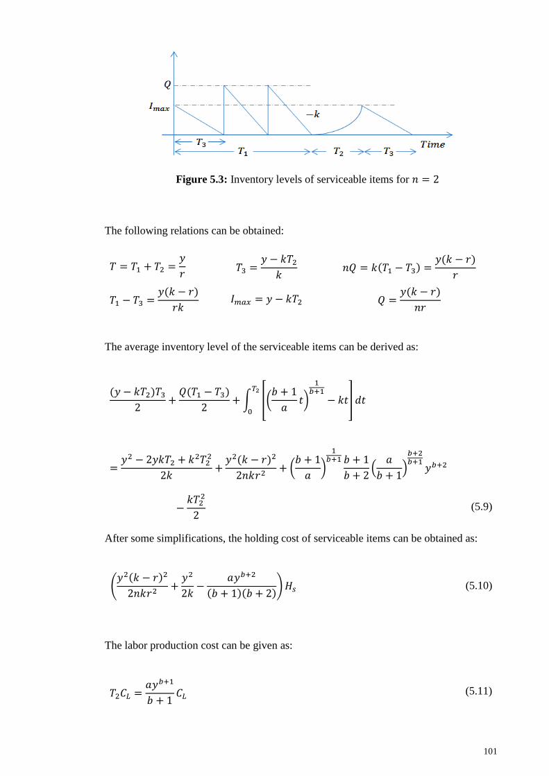
101

Figure 5.3: Inventory levels of serviceable items for 𝑛 = 2

The following relations can be obtained:

𝑇 = 𝑇1 + 𝑇2 =𝑦

𝑟 𝑇3 =

𝑦 − 𝑘𝑇2𝑘

𝑛𝑄 = 𝑘(𝑇1 − 𝑇3) =𝑦(𝑘 − 𝑟)

𝑟

𝑇1 − 𝑇3 =𝑦(𝑘 − 𝑟)

𝑟𝑘 𝐼𝑚𝑎𝑥 = 𝑦 − 𝑘𝑇2 𝑄 =

𝑦(𝑘 − 𝑟)

𝑛𝑟

The average inventory level of the serviceable items can be derived as:

(𝑦 − 𝑘𝑇2)𝑇32

+𝑄(𝑇1 − 𝑇3)

2+ ∫ [(

𝑏 + 1

𝑎𝑡)

1𝑏+1

− 𝑘𝑡] 𝑑𝑡𝑇2

0

=𝑦2 − 2𝑦𝑘𝑇2 + 𝑘

2𝑇22

2𝑘+𝑦2(𝑘 − 𝑟)2

2𝑛𝑘𝑟2+ (

𝑏 + 1

𝑎)

1𝑏+1 𝑏 + 1

𝑏 + 2(𝑎

𝑏 + 1)

𝑏+2𝑏+1

𝑦𝑏+2

−𝑘𝑇2

2

2

(5.9)

After some simplifications, the holding cost of serviceable items can be obtained as:

(𝑦2(𝑘 − 𝑟)2

2𝑛𝑘𝑟2+𝑦2

2𝑘−

𝑎𝑦𝑏+2

(𝑏 + 1)(𝑏 + 2))𝐻𝑠 (5.10)

The labor production cost can be given as:

𝑇2𝐶𝐿 =𝑎𝑦𝑏+1

𝑏 + 1𝐶𝐿 (5.11)

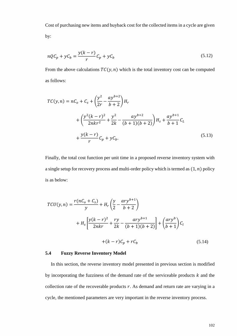
102

Cost of purchasing new items and buyback cost for the collected items in a cycle are given

by:

𝑛𝑄𝐶𝑝 + 𝑦𝐶𝑏 =𝑦(𝑘 − 𝑟)

𝑟𝐶𝑝 + 𝑦𝐶𝑏 (5.12)

From the above calculations 𝑇𝐶(𝑦, 𝑛) which is the total inventory cost can be computed

as follows:

𝑇𝐶(𝑦, 𝑛) = 𝑛𝐶𝑜 + 𝐶𝑠 + (𝑦2


𝑏 + 2)𝐻𝑟

+ (𝑦2(𝑘 − 𝑟)2

2𝑛𝑘𝑟2+𝑦2

2𝑘−

𝑎𝑦𝑏+2

(𝑏 + 1)(𝑏 + 2))𝐻𝑠 +

𝑎𝑦𝑏+1

𝑏 + 1𝐶𝐿

+𝑦(𝑘 − 𝑟)

𝑟𝐶𝑝 + 𝑦𝐶𝑏 .

(5.13)

Finally, the total cost function per unit time in a proposed reverse inventory system with

a single setup for recovery process and multi-order policy which is termed as (1, 𝑛) policy

is as below:

𝑇𝐶𝑈(𝑦, 𝑛) =𝑟(𝑛𝐶𝑜 + 𝐶𝑠)

𝑦+ 𝐻𝑟 (

𝑦

2−𝑎𝑟𝑦𝑏+1

𝑏 + 2)

+ 𝐻𝑠 [𝑦(𝑘 − 𝑟)2

2𝑛𝑘𝑟+𝑟𝑦

2𝑘−

𝑎𝑟𝑦𝑏+1

(𝑏 + 1)(𝑏 + 2)] + (

𝑎𝑟𝑦𝑏

𝑏 + 1)𝐶𝑙

+(𝑘 − 𝑟)𝐶𝑝 + 𝑟𝐶𝑏 (5.14)

5.4 Fuzzy Reverse Inventory Model

In this section, the reverse inventory model presented in previous section is modified

by incorporating the fuzziness of the demand rate of the serviceable products 𝑘 and the

collection rate of the recoverable products 𝑟. As demand and return rate are varying in a

cycle, the mentioned parameters are very important in the reverse inventory process.

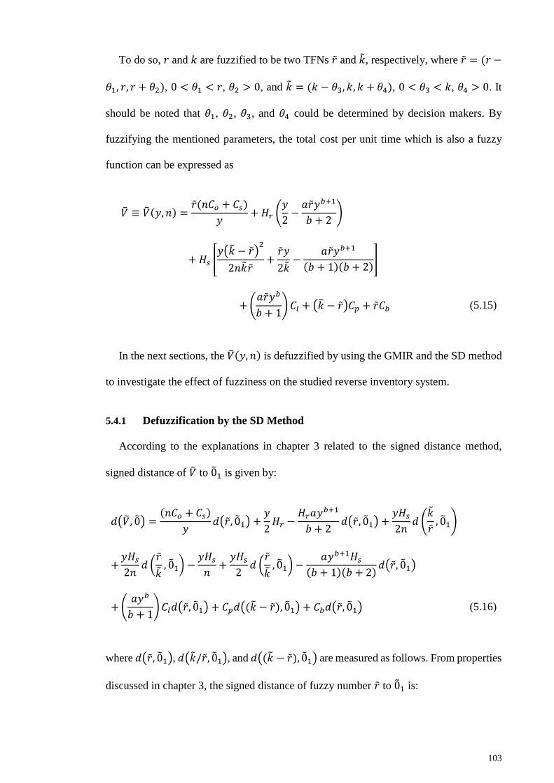
103

To do so, 𝑟 and 𝑘 are fuzzified to be two TFNs �̃� and �̃�, respectively, where �̃� = (𝑟 −

𝜃1, 𝑟, 𝑟 + 𝜃2), 0 < 𝜃1 < 𝑟, 𝜃2 > 0, and �̃� = (𝑘 − 𝜃3, 𝑘, 𝑘 + 𝜃4), 0 < 𝜃3 < 𝑘, 𝜃4 > 0. It

should be noted that 𝜃1, 𝜃2, 𝜃3, and 𝜃4 could be determined by decision makers. By

fuzzifying the mentioned parameters, the total cost per unit time which is also a fuzzy

function can be expressed as

�̃� ≡ �̃�(𝑦, 𝑛) =�̃�(𝑛𝐶𝑜 + 𝐶𝑠)

𝑦+ 𝐻𝑟 (

𝑦

2−𝑎�̃�𝑦𝑏+1

𝑏 + 2)

+ 𝐻𝑠 [𝑦(�̃� − �̃�)

2

2𝑛�̃��̃�+�̃�𝑦

2�̃�−

𝑎�̃�𝑦𝑏+1

(𝑏 + 1)(𝑏 + 2)]

+(𝑎�̃�𝑦𝑏

𝑏 + 1)𝐶𝑙 + (�̃� − �̃�)𝐶𝑝 + �̃�𝐶𝑏 (5.15)

In the next sections, the �̃�(𝑦, 𝑛) is defuzzified by using the GMIR and the SD method

to investigate the effect of fuzziness on the studied reverse inventory system.

5.4.1 Defuzzification by the SD Method

According to the explanations in chapter 3 related to the signed distance method,

signed distance of �̃� to 0̃1 is given by:

𝑑(�̃�, 0̃) =(𝑛𝐶𝑜 + 𝐶𝑠)

𝑦𝑑(�̃�, 0̃1) +

𝑦

2𝐻𝑟 −

𝐻𝑟𝑎𝑦𝑏+1

𝑏 + 2𝑑(�̃�, 0̃1) +

𝑦𝐻𝑠2𝑛

𝑑 (�̃�

�̃�, 0̃1)

+𝑦𝐻𝑠2𝑛

𝑑 (�̃�

�̃�, 0̃1) −

𝑦𝐻𝑠𝑛+𝑦𝐻𝑠2𝑑 (�̃�

�̃�, 0̃1) −

𝑎𝑦𝑏+1𝐻𝑠(𝑏 + 1)(𝑏 + 2)

𝑑(�̃�, 0̃1)

+(𝑎𝑦𝑏

𝑏 + 1)𝐶𝑙𝑑(�̃�, 0̃1) + 𝐶𝑝𝑑((�̃� − �̃�), 0̃1) + 𝐶𝑏𝑑(�̃�, 0̃1) (5.16)

where 𝑑(�̃�, 0̃1), 𝑑(�̃�/�̃�, 0̃1), and 𝑑((�̃� − �̃�), 0̃1) are measured as follows. From properties

discussed in chapter 3, the signed distance of fuzzy number �̃� to 0̃1 is:

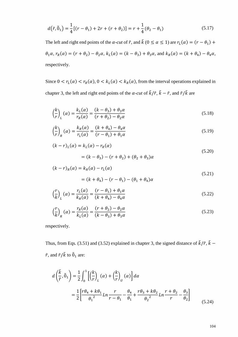
104

𝑑(�̃�, 0̃1) =1

4[(𝑟 − 𝜃1) + 2𝑟 + (𝑟 + 𝜃2)] = 𝑟 +

1

4(𝜃2 − 𝜃1) (5.17)

The left and right end points of the 𝛼-cut of �̃�, and �̃� (0 ≤ 𝛼 ≤ 1) are 𝑟𝐿(𝛼) = (𝑟 − 𝜃1) +

𝜃1𝛼, 𝑟𝑅(𝛼) = (𝑟 + 𝜃2) − 𝜃2𝛼, 𝑘𝐿(𝛼) = (𝑘 − 𝜃3) + 𝜃3𝛼, and 𝑘𝑅(𝛼) = (𝑘 + 𝜃4) − 𝜃4𝛼,

respectively.

Since 0 < 𝑟𝐿(𝛼) < 𝑟𝑅(𝛼), 0 < 𝑘𝐿(𝛼) < 𝑘𝑅(𝛼), from the interval operations explained in

chapter 3, the left and right end points of the 𝛼-cut of �̃�/�̃�, �̃� − �̃�, and �̃�/�̃� are

(𝑘

𝑟)𝐿

(𝛼) =𝑘𝐿(𝛼)

𝑟𝑅(𝛼)=(𝑘 − 𝜃3) + 𝜃3𝛼

(𝑟 + 𝜃2) − 𝜃2𝛼 (5.18)

(𝑘

𝑟)𝑅

(𝛼) =𝑘𝑅(𝛼)

𝑟𝐿(𝛼)=(𝑘 + 𝜃4) − 𝜃4𝛼

(𝑟 − 𝜃1) + 𝜃1𝛼 (5.19)

(𝑘 − 𝑟)𝐿(𝛼) = 𝑘𝐿(𝛼) − 𝑟𝑅(𝛼)

= (𝑘 − 𝜃3) − (𝑟 + 𝜃2) + (𝜃2 + 𝜃3)𝛼

(5.20)

(𝑘 − 𝑟)𝑅(𝛼) = 𝑘𝑅(𝛼) − 𝑟𝐿(𝛼)

= (𝑘 + 𝜃4) − (𝑟 − 𝜃1) − (𝜃1 + 𝜃4)𝛼

(5.21)

(𝑟

𝑘)𝐿(𝛼) =

𝑟𝐿(𝛼)

𝑘𝑅(𝛼)=(𝑟 − 𝜃1) + 𝜃1𝛼

(𝑘 + 𝜃4) − 𝜃4𝛼 (5.22)

(𝑟

𝑘)𝑅(𝛼) =

𝑟𝑅(𝛼)

𝑘𝐿(𝛼)=(𝑟 + 𝜃2) − 𝜃2𝛼

(𝑘 − 𝜃3) + 𝜃3𝛼 (5.23)

respectively.

Thus, from Eqs. (3.51) and (3.52) explained in chapter 3, the signed distance of �̃�/�̃�, �̃� −

�̃�, and �̃�/�̃� to 0̃1 are:

𝑑 (�̃�

�̃�, 0̃1) =

1

2∫ [(

𝑘

𝑟)𝐿

(𝛼) + (𝑘

𝑟)𝑈

(𝛼)]1

0

𝑑𝛼

=1

2[𝑟𝜃4 + 𝑘𝜃1

𝜃12 𝐿𝑛

𝑟

𝑟 − 𝜃1−𝜃4𝜃1+𝑟𝜃3 + 𝑘𝜃2

𝜃22 𝐿𝑛

𝑟 + 𝜃2𝑟

−𝜃3𝜃2]

(5.24)

105

𝑑 (�̃�

�̃�, 0̃1) =

1

2∫ [(

𝑟

𝑘)𝐿(𝛼) + (

𝑟

𝑘)𝑈(𝛼)]

1

0

𝑑𝛼

=1

2[𝑘𝜃2 + 𝑟𝜃3

𝜃32 𝐿𝑛

𝑘

𝑘 − 𝜃3−𝜃2𝜃3+𝑘𝜃1 + 𝑟𝜃4

𝜃42 𝐿𝑛

𝑘 + 𝜃4𝑘

−𝜃1𝜃4]

(5.25)

𝑑 ((�̃� − �̃�), 0̃1) =1

2∫ [(𝑘 − 𝑟)𝐿(𝛼) + (𝑘 − 𝑟)𝑈(𝛼)]1

0

𝑑𝛼

=1

2([(𝜃2 + 𝜃3) − (𝜃1 + 𝜃4)]

1

2+ (𝑘 − 𝜃3) + (𝑘 + 𝜃4)

− (𝑟 + 𝜃2) − (𝑟 − 𝜃1))

(5.26)

respectively. Substituting the results obtained by (5.24)-( 5.26) into (5.16), we have

𝑉(𝑛, 𝑦) ≡ 𝑑(�̃�, 0̃)

= 𝑑(�̃�, 0̃1) [(𝑛𝐶𝑜 + 𝐶𝑠)

𝑦−𝐻𝑟𝑎𝑦

𝑏+1

𝑏 + 2−

𝑎𝑦𝑏+1𝐻𝑠(𝑏 + 1)(𝑏 + 2)

+ (𝑎𝑦𝑏

𝑏 + 1)𝐶𝑙

+ 𝐶𝑏]

+𝑑 (�̃�

�̃�, 0̃1)

𝑦𝐻𝑠2𝑛

+ 𝑑 (�̃�

�̃�, 0̃1) [

𝑦𝐻𝑠2𝑛

+𝑦𝐻𝑠2] + 𝑑((�̃� − �̃�), 0̃1)𝐶𝑝

−𝑦𝐻𝑠𝑛+𝑦

2𝐻𝑟

(5.27)

By replacing the related terms, we have:

𝑉(𝑛, 𝑦) ≡ 𝑑(�̃�, 0̃)

= [𝑟 +1

4(𝜃2 − 𝜃1)]

. [(𝑛𝐶𝑜 + 𝐶𝑠)

𝑦−𝐻𝑟𝑎𝑦

𝑏+1

𝑏 + 2−

𝑎𝑦𝑏+1𝐻𝑠(𝑏 + 1)(𝑏 + 2)

+ (𝑎𝑦𝑏

𝑏 + 1)𝐶𝑙 + 𝐶𝑏]

+𝑦𝐻𝑠4𝑛

[𝑟𝜃4 + 𝑘𝜃1

𝜃12 𝐿𝑛

𝑟

𝑟 − 𝜃1−𝜃4𝜃1+𝑟𝜃3 + 𝑘𝜃2

𝜃22 𝐿𝑛

𝑟 + 𝜃2𝑟

−𝜃3𝜃2]

+(1 + 𝑛)𝑦𝐻𝑠

4𝑛[𝑘𝜃2 + 𝑟𝜃3

𝜃32 𝐿𝑛

𝑘

𝑘 − 𝜃3−𝜃2𝜃3+𝑘𝜃1 + 𝑟𝜃4

𝜃42 𝐿𝑛

𝑘 + 𝜃4𝑘

−𝜃1𝜃4]

106

+(𝑘 − 𝑟 −𝜃2 + 𝜃3 − 𝜃1 − 𝜃4

4)𝐶𝑝 −

𝑦𝐻𝑠𝑛+𝑦

2𝐻𝑟 (5.28)

𝑉(𝑛, 𝑦) is considered as the estimate of the total cost per unit time in fuzzy situation.

The next step is to determine the optimal recovery lot size to minimize the total cost

function 𝑉(𝑛, 𝑦). By setting the first derivative of 𝑑(�̃�, 0̃) with respect to 𝑛 equal to zero,

𝑦 can be obtained as follow:

𝜕𝑑(�̃�, 0̃)

𝜕𝑛= 0 → 𝑦 = 𝑛√

2𝐶𝑜𝑑(�̃�, 0̃1)

𝐻𝑠∆= 𝑛𝜌 (5.29)

where

∆= 𝑑 (�̃�

�̃�, 0̃1) + 𝑑 (

�̃�

�̃�, 0̃1) − 2 and 𝜌 = √

2𝐶𝑜𝑑(�̃�, 0̃1)

𝐻𝑠∆

By setting the first derivative of 𝑑(�̃�, 0̃) with respect to 𝑦, we have:

𝜕𝑑(�̃�, 0̃)

𝜕𝑦= −

(𝑛𝐶𝑜 + 𝐶𝑠)

𝑦2𝑑(�̃�, 0̃1) +

1

2𝐻𝑟

−(𝑏 + 1)𝐻𝑟𝑎𝑦

𝑏

𝑏 + 2𝑑(�̃�, 0̃1) +

𝐻𝑠2𝑛𝑑 (�̃�

�̃�, 0̃1)

+𝐻𝑠2𝑛𝑑 (�̃�

�̃�, 0̃1) −

𝐻𝑠𝑛+𝐻𝑠2𝑑 (�̃�

�̃�, 0̃1) −

𝑎𝑦𝑏𝐻𝑠(𝑏 + 2)

𝑑(�̃�, 0̃1)

+(𝑎𝑏𝑦𝑏−1

𝑏 + 1)𝐶𝑙𝑑(�̃�, 0̃1) = 0 (5.30)

and after substituting 𝑦 from (5.29) into (5.30), �̃�(𝑛) can be derived as

�̃�(𝑛) = −(𝑛𝐶𝑜 + 𝐶𝑠)

𝑛2𝜌2𝑑(�̃�, 0̃1) +

1

2𝐻𝑟 −

(𝑏 + 1)𝐻𝑟𝑎𝑛𝑏𝜌𝑏

𝑏 + 2𝑑(�̃�, 0̃1) +

𝐻𝑠2𝑛

107

+𝐻𝑠2𝑛(𝑑 (

�̃�

�̃�, 0̃1) + 𝑑 (

�̃�

�̃�, 0̃1) − 2) +

𝐻𝑠2𝑑 (�̃�

�̃�, 0̃1)

−𝑎𝑛𝑏𝜌𝑏𝐻𝑠(𝑏 + 2)

𝑑(�̃�, 0̃1) + (𝑎𝑏𝑛𝑏−1𝜌𝑏−1

𝑏 + 1)𝐶𝑙𝑑(�̃�, 0̃1)

(5.31)

5.4.2 Finding the Optimal Values for the SD Method

Letting (𝑦∗,𝑛∗) shows the solution for the considered problem. To prove that 𝑦∗ and𝑛∗

are the optimal recovery lot size and the optimal number of orders, respectively, Theorem

1 and 2 are necessary.

Theorem 1: The optimal solution of (𝑦∗,𝑛∗) not only exists, but is also unique. It is clear

that it should satisfy �̃�(𝑛) = 0, and 𝑦 − 𝑛𝜌 = 0, simultaneously.

Proof. By taking the first derivative of the �̃�(𝑛) with respect to 𝑛, we have:

𝜕�̃�(𝑛)

𝜕𝑛= 𝑏(𝛽′ + 𝛿′)𝑛𝑏−1 −

2𝛼′

𝑛3+ (𝑏 − 1)휁′𝑛𝑏−2 −

𝛾′

𝑛2> 0 (5.32)

where

𝛼′ = −(𝑛𝐶𝑜 + 𝐶𝑠)𝐻𝑠∆

2𝐶𝑜

𝛽′ = −(𝑏 + 1)𝐻𝑟𝑎𝜌

𝑏

𝑏 + 2𝑑(�̃�, 0̃1)

𝛾′ =𝐻𝑠2∆

𝛿′ = −𝑎𝜌𝑏𝐻𝑠(𝑏 + 2)

𝑑(�̃�, 0̃1)

휁′ = (𝑎𝑏𝜌𝑏−1

𝑏 + 1)𝐶𝑙𝑑(�̃�, 0̃1)

휀′ =1

2𝐻𝑟 +

𝐻𝑠2𝑑 (�̃�

�̃�, 0̃1)

108

It is positive for all value of 𝑛 > 0. Hence, �̃�(𝑛) is a strictly increasing function for

0 < 𝑛 < ∞. Moreover, there are the following limitations:

lim𝑛→+∞

�̃�(𝑛) = 휀′ > 0

lim𝑛→0+

�̃�(𝑛) = −∞

Thus, by the Intermediate Value Theorem introduced in chapter 3, there exists a unique

0 < 𝑛∗ < ∞ such that �̃�(𝑛∗) = 0.

Theorem 2: 𝑑(�̃�, 0̃) has a global minimum at (𝑦∗,𝑛∗), where this point is the solution

for �̃�(𝑛) = 0, and 𝑦 − 𝑛𝜌 = 0.

Proof. From Theorem 1, it is clear that (𝑦∗, 𝑛∗) is the only critical point. Therefore, to

prove the Theorem 2, the Hessian Matrix of 𝑑(�̃�, 0̃) should firstly be calculated as

follows:

𝜕2𝑑(�̃�, 0̃)

𝜕𝑦2=𝜕2𝑉(𝑛, 𝑦)

𝜕𝑦2

=2(𝑛𝐶𝑜 + 𝐶𝑠)

𝑦3𝑑(�̃�, 0̃1) −

𝑏(𝑏 + 1)𝐻𝑟𝑎𝑦𝑏−1

𝑏 + 2𝑑(�̃�, 0̃1)

−𝑏𝑎𝑦𝑏−1𝐻𝑠(𝑏 + 2)

𝑑(�̃�, 0̃1)

+ ((𝑏 − 1)𝑎𝑏𝑦𝑏−2

𝑏 + 1)𝐶𝑙𝑑(�̃�, 0̃1)

(5.33)

For all 𝑦 > 0, 𝑛 > 0, 𝜕2𝑑(�̃�, 0̃) 𝜕𝑦2⁄ > 0

𝜕2𝑑(�̃�, 0̃)

𝜕𝑛2=𝑦𝐻𝑠𝑛3

∆ (5.34)

For all 𝑦 > 0, 𝑛 > 0, 𝜕2𝑑(�̃�, 0̃) 𝜕𝑛2⁄ > 0.

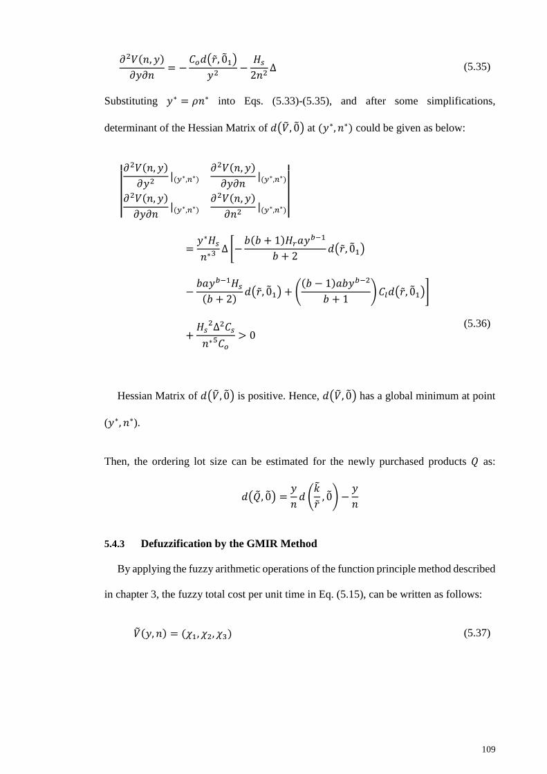
109

𝜕2𝑉(𝑛, 𝑦)

𝜕𝑦𝜕𝑛= −

𝐶𝑜𝑑(�̃�, 0̃1)

𝑦2−𝐻𝑠2𝑛2

∆ (5.35)

Substituting 𝑦∗ = 𝜌𝑛∗ into Eqs. (5.33)-(5.35), and after some simplifications,

determinant of the Hessian Matrix of 𝑑(�̃�, 0̃) at (𝑦∗, 𝑛∗) could be given as below:

||

𝜕2𝑉(𝑛, 𝑦)

𝜕𝑦2|(𝑦∗,𝑛∗)

𝜕2𝑉(𝑛, 𝑦)

𝜕𝑦𝜕𝑛|(𝑦∗,𝑛∗)

𝜕2𝑉(𝑛, 𝑦)

𝜕𝑦𝜕𝑛|(𝑦∗,𝑛∗)

𝜕2𝑉(𝑛, 𝑦)

𝜕𝑛2|(𝑦∗,𝑛∗)

||

=𝑦∗𝐻𝑠

𝑛∗3∆ [−

𝑏(𝑏 + 1)𝐻𝑟𝑎𝑦𝑏−1

𝑏 + 2𝑑(�̃�, 0̃1)

−𝑏𝑎𝑦𝑏−1𝐻𝑠(𝑏 + 2)

𝑑(�̃�, 0̃1) + ((𝑏 − 1)𝑎𝑏𝑦𝑏−2

𝑏 + 1)𝐶𝑙𝑑(�̃�, 0̃1)]

+𝐻𝑠

2∆2𝐶𝑠

𝑛∗5𝐶𝑜> 0

(5.36)

Hessian Matrix of 𝑑(�̃�, 0̃) is positive. Hence, 𝑑(�̃�, 0̃) has a global minimum at point

(𝑦∗, 𝑛∗).

Then, the ordering lot size can be estimated for the newly purchased products 𝑄 as:

𝑑(�̃�, 0̃) =𝑦

𝑛𝑑 (�̃�

�̃�, 0̃) −

𝑦

𝑛

5.4.3 Defuzzification by the GMIR Method

By applying the fuzzy arithmetic operations of the function principle method described

in chapter 3, the fuzzy total cost per unit time in Eq. (5.15), can be written as follows:

�̃�(𝑦, 𝑛) = (𝜒1, 𝜒2, 𝜒3) (5.37)

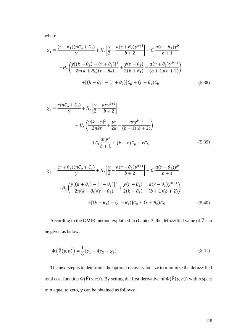
110

where

𝜒1 =(𝑟 − 𝜃1)(𝑛𝐶𝑜 + 𝐶𝑠)

𝑦+ 𝐻𝑟 [

𝑦

2−𝑎(𝑟 + 𝜃2)𝑦

𝑏+1

𝑏 + 2]+ 𝐶𝑙

𝑎(𝑟 − 𝜃1)𝑦𝑏

𝑏 + 1

+𝐻𝑠 (𝑦[(𝑘 − 𝜃3) − (𝑟 + 𝜃2)]

2

2𝑛(𝑘 + 𝜃4)(𝑟 + 𝜃2)+𝑦(𝑟 − 𝜃1)

2(𝑘 + 𝜃4)−𝑎(𝑟 + 𝜃2)𝑦

𝑏+1

(𝑏 + 1)(𝑏 + 2))

+[(𝑘 − 𝜃3) − (𝑟 + 𝜃2)]𝐶𝑝 + (𝑟 − 𝜃1)𝐶𝑏 (5.38)

𝜒2 =𝑟(𝑛𝐶𝑜 + 𝐶𝑠)

𝑦+𝐻𝑟 [

𝑦

2−𝑎𝑟𝑦𝑏+1

𝑏 + 2]

+𝐻𝑠 (𝑦[𝑘 − 𝑟]2

2𝑛𝑘𝑟+𝑦𝑟

2𝑘−

𝑎𝑟𝑦𝑏+1

(𝑏 + 1)(𝑏 + 2))

+𝐶𝑙𝑎𝑟𝑦𝑏

𝑏 + 1+ (𝑘 − 𝑟)𝐶𝑝 + 𝑟𝐶𝑏 (5.39)

𝜒3 =(𝑟 + 𝜃2)(𝑛𝐶𝑜 + 𝐶𝑠)

𝑦+ 𝐻𝑟 [

𝑦

2−𝑎(𝑟 − 𝜃1)𝑦

𝑏+1

𝑏 + 2]+ 𝐶𝑙

𝑎(𝑟 + 𝜃2)𝑦𝑏

𝑏 + 1

+𝐻𝑠 (𝑦[(𝑘 + 𝜃4) − (𝑟 − 𝜃1)]

2

2𝑛(𝑘 − 𝜃3)(𝑟 − 𝜃1)+𝑦(𝑟 + 𝜃2)

2(𝑘 − 𝜃3)−𝑎(𝑟 − 𝜃1)𝑦

𝑏+1

(𝑏 + 1)(𝑏 + 2))

+[(𝑘 + 𝜃4) − (𝑟 − 𝜃1)]𝐶𝑝 + (𝑟 + 𝜃2)𝐶𝑏 (5.40)

According to the GMIR method explained in chapter 3, the defuzzified value of �̃� can

be given as below:

Φ(�̃�(𝑦, 𝑛)) =1

6(𝜒1 + 4𝜒2 + 𝜒3) (5.41)

The next step is to determine the optimal recovery lot size to minimize the defuzzified

total cost function Φ(�̃�(𝑦, 𝑛)). By setting the first derivative of Φ(�̃�(𝑦, 𝑛)) with respect

to 𝑛 equal to zero, 𝑦 can be obtained as follows:

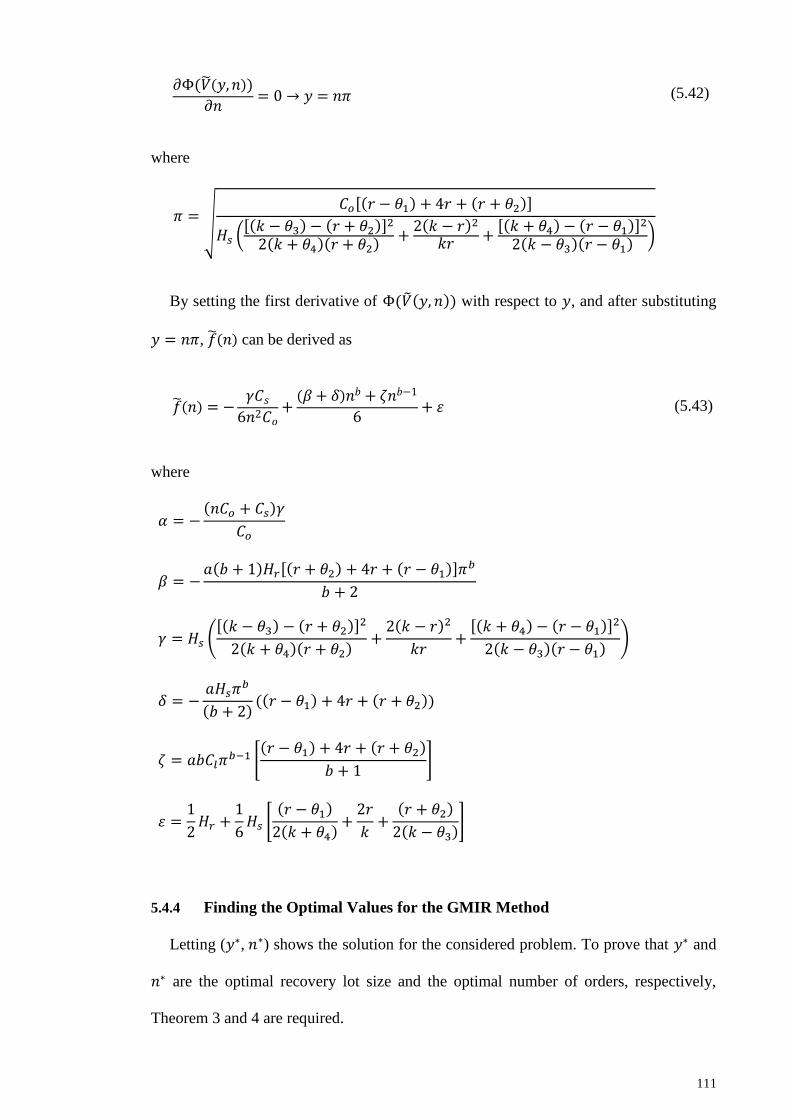
111

𝜕Φ(�̃�(𝑦, 𝑛))

𝜕𝑛= 0 → 𝑦 = 𝑛𝜋 (5.42)

where

𝜋 = √

𝐶𝑜[(𝑟 − 𝜃1) + 4𝑟 + (𝑟 + 𝜃2)]

𝐻𝑠 ([(𝑘 − 𝜃3) − (𝑟 + 𝜃2)]2

2(𝑘 + 𝜃4)(𝑟 + 𝜃2)+2(𝑘 − 𝑟)2

𝑘𝑟+[(𝑘 + 𝜃4) − (𝑟 − 𝜃1)]2

2(𝑘 − 𝜃3)(𝑟 − 𝜃1))

By setting the first derivative of Φ(�̃�(𝑦, 𝑛)) with respect to 𝑦, and after substituting

𝑦 = 𝑛𝜋, �̃�(𝑛) can be derived as

�̃�(𝑛) = −𝛾𝐶𝑠6𝑛2𝐶𝑜

+(𝛽 + 𝛿)𝑛𝑏 + 휁𝑛𝑏−1

6+ 휀 (5.43)

where

𝛼 = −(𝑛𝐶𝑜 + 𝐶𝑠)𝛾

𝐶𝑜

𝛽 = −𝑎(𝑏 + 1)𝐻𝑟[(𝑟 + 𝜃2) + 4𝑟 + (𝑟 − 𝜃1)]𝜋

𝑏

𝑏 + 2

𝛾 = 𝐻𝑠 ([(𝑘 − 𝜃3) − (𝑟 + 𝜃2)]

2

2(𝑘 + 𝜃4)(𝑟 + 𝜃2)+2(𝑘 − 𝑟)2

𝑘𝑟+[(𝑘 + 𝜃4) − (𝑟 − 𝜃1)]

2

2(𝑘 − 𝜃3)(𝑟 − 𝜃1))

𝛿 = −𝑎𝐻𝑠𝜋

𝑏

(𝑏 + 2)((𝑟 − 𝜃1) + 4𝑟 + (𝑟 + 𝜃2))

휁 = 𝑎𝑏𝐶𝑙𝜋𝑏−1 [

(𝑟 − 𝜃1) + 4𝑟 + (𝑟 + 𝜃2)

𝑏 + 1]

휀 =1

2𝐻𝑟 +

1

6𝐻𝑠 [

(𝑟 − 𝜃1)

2(𝑘 + 𝜃4)+2𝑟

𝑘+(𝑟 + 𝜃2)

2(𝑘 − 𝜃3)]

5.4.4 Finding the Optimal Values for the GMIR Method

Letting (𝑦∗,𝑛∗) shows the solution for the considered problem. To prove that 𝑦∗ and

𝑛∗ are the optimal recovery lot size and the optimal number of orders, respectively,

Theorem 3 and 4 are required.

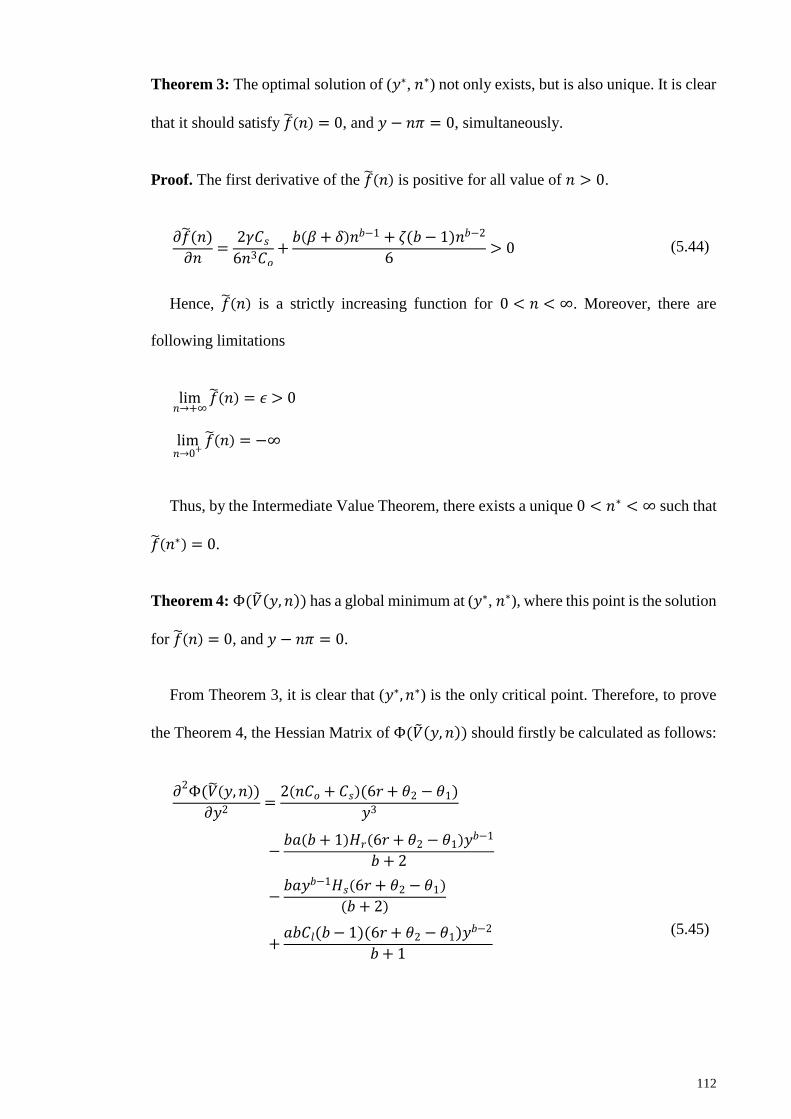
112

Theorem 3: The optimal solution of (𝑦∗,𝑛∗) not only exists, but is also unique. It is clear

that it should satisfy �̃�(𝑛) = 0, and 𝑦 − 𝑛𝜋 = 0, simultaneously.

Proof. The first derivative of the �̃�(𝑛) is positive for all value of 𝑛 > 0.

𝜕�̃�(𝑛)

𝜕𝑛=2𝛾𝐶𝑠6𝑛3𝐶𝑜

+𝑏(𝛽 + 𝛿)𝑛𝑏−1 + 휁(𝑏 − 1)𝑛𝑏−2

6> 0 (5.44)

Hence, �̃�(𝑛) is a strictly increasing function for 0 < 𝑛 < ∞. Moreover, there are

following limitations

lim𝑛→+∞

�̃�(𝑛) = 𝜖 > 0

lim𝑛→0+

�̃�(𝑛) = −∞

Thus, by the Intermediate Value Theorem, there exists a unique 0 < 𝑛∗ < ∞ such that

�̃�(𝑛∗) = 0.

Theorem 4: Φ(�̃�(𝑦, 𝑛)) has a global minimum at (𝑦∗,𝑛∗), where this point is the solution

for �̃�(𝑛) = 0, and 𝑦 − 𝑛𝜋 = 0.

From Theorem 3, it is clear that (𝑦∗, 𝑛∗) is the only critical point. Therefore, to prove

the Theorem 4, the Hessian Matrix of Φ(�̃�(𝑦, 𝑛)) should firstly be calculated as follows:

𝜕2Φ(�̃�(𝑦, 𝑛))

𝜕𝑦2=2(𝑛𝐶𝑜 + 𝐶𝑠)(6𝑟 + 𝜃2 − 𝜃1)

𝑦3

−𝑏𝑎(𝑏 + 1)𝐻𝑟(6𝑟 + 𝜃2 − 𝜃1)𝑦

𝑏−1

𝑏 + 2

−𝑏𝑎𝑦𝑏−1𝐻𝑠(6𝑟 + 𝜃2 − 𝜃1)

(𝑏 + 2)

+𝑎𝑏𝐶𝑙(𝑏 − 1)(6𝑟 + 𝜃2 − 𝜃1)𝑦

𝑏−2

𝑏 + 1

(5.45)

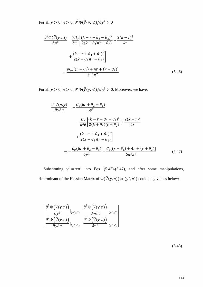
113

For all 𝑦 > 0, 𝑛 > 0, 𝜕2Φ(�̃�(𝑦, 𝑛)) 𝜕𝑦2⁄ > 0

𝜕2Φ(�̃�(𝑦, 𝑛))

𝜕𝑛2=𝑦𝐻𝑠3𝑛3

[(𝑘 − 𝑟 − 𝜃3 − 𝜃2)

2

2(𝑘 + 𝜃4)(𝑟 + 𝜃2)+2(𝑘 − 𝑟)2

𝑘𝑟

+(𝑘 − 𝑟 + 𝜃4 + 𝜃1)

2

2(𝑘 − 𝜃3)(𝑟 − 𝜃1)]

=𝑦𝐶𝑜[(𝑟 − 𝜃1) + 4𝑟 + (𝑟 + 𝜃2)]

3𝑛3𝜋2 (5.46)

For all 𝑦 > 0, 𝑛 > 0, 𝜕2Φ(�̃�(𝑦, 𝑛)) 𝜕𝑛2⁄ > 0. Moreover, we have:

𝜕2𝑉(𝑛, 𝑦)

𝜕𝑦𝜕𝑛= −

𝐶𝑜(6𝑟 + 𝜃2 − 𝜃1)

6𝑦2

−𝐻𝑠𝑛26

[(𝑘 − 𝑟 − 𝜃3 − 𝜃2)

2

2(𝑘 + 𝜃4)(𝑟 + 𝜃2)+2(𝑘 − 𝑟)2

𝑘𝑟

+(𝑘 − 𝑟 + 𝜃4 + 𝜃1)

2

2(𝑘 − 𝜃3)(𝑟 − 𝜃1)]

= −𝐶𝑜(6𝑟 + 𝜃2 − 𝜃1)

6𝑦2−𝐶𝑜[(𝑟 − 𝜃1) + 4𝑟 + (𝑟 + 𝜃2)]

6𝑛2𝜋2 (5.47)

Substituting 𝑦∗ = 𝜋𝑛∗ into Eqs. (5.45)-(5.47), and after some manipulations,

determinant of the Hessian Matrix of Φ(�̃�(𝑦, 𝑛)) at (𝑦∗, 𝑛∗) could be given as below:

|

|

𝜕2Φ (�̃�(𝑦, 𝑛))

𝜕𝑦2|(𝑦∗,𝑛∗)

𝜕2Φ (�̃�(𝑦, 𝑛))

𝜕𝑦𝜕𝑛|(𝑦∗,𝑛∗)

𝜕2Φ (�̃�(𝑦, 𝑛))

𝜕𝑦𝜕𝑛|(𝑦∗,𝑛∗)

𝜕2Φ (�̃�(𝑦, 𝑛))

𝜕𝑛2|(𝑦∗,𝑛∗)

|

|

(5.48)

114

=𝑦∗𝐶𝑜(6𝑟 + 𝜃2 − 𝜃1)

3𝑛∗3𝜋2[−𝑏𝑎(𝑏 + 1)𝐻𝑟(6𝑟 + 𝜃2 − 𝜃1)𝑦

𝑏−1

𝑏 + 2

−𝑏𝑎𝑦𝑏−1𝐻𝑠(6𝑟 + 𝜃2 − 𝜃1)

(𝑏 + 2)

+𝑎𝑏𝐶𝑙(𝑏 − 1)(6𝑟 + 𝜃2 − 𝜃1)𝑦

𝑏−2

𝑏 + 1]

+𝐶𝑜(6𝑟 + 𝜃2 − 𝜃1)

2(5𝑛𝐶𝑜 + 6𝐶𝑠)

9𝑛∗5𝜋4> 0

Hessian Matrix of Φ(�̃�(𝑦, 𝑛)) is positive. Hence, Φ(�̃�(𝑦, 𝑛)) has a global minimum

at point (𝑦∗, 𝑛∗).

Therefore, ordering lot size can be estimated for the newly purchased products 𝑄 as

Φ(�̃�) =1

6(𝑞1 + 4𝑞2 + 𝑞3)

=1

6(𝑦[(𝑘 − 𝜃3) − (𝑟 + 𝜃2)]

𝑛(𝑟 + 𝜃2)+4𝑦(𝑘 − 𝑟)

𝑛𝑟+𝑦[(𝑘 + 𝜃4) − (𝑟 − 𝜃1)]

𝑛(𝑟 − 𝜃1))

5.5 Solution Procedure

Finding a closed-form solution is not possible for �̃�(𝑛) = 0 or �̃�(𝑛) = 0. Instead of a

direct method, 𝑛∗ can be found by a one-dimensional search procedure. When 𝑛∗ can be

found, 𝑦∗ can be obtained by 𝜕𝑑(�̃�, 0̃)/𝜕𝑦 = 0. As 𝑛∗ is a positive integer, the following

solution algorithm can also be applied to find the optimal values.

5.6 One-dimensional Search Procedure for Optimization

The obtained defuzzified functions can be optimized through a heuristic mathematical

algorithm explained in this section as depicted in Figure 5.4.

Consider a pre-determined error value 𝜏 > 0. Set 𝑛𝑙 and 𝑛𝑢 as suggested guesses of

the root such that 𝑓(𝑛𝑢) > 0 and 𝑓(𝑛𝑙) < 0. The optimal values for both methods (i.e.

GMIR method and SD method) could be found by the proposed flowchart in Figure 5.4.

In this flowchart, ⌊𝑛⌋ and ⌈𝑛⌉ show the nearest integers smaller and larger than 𝑛∗.

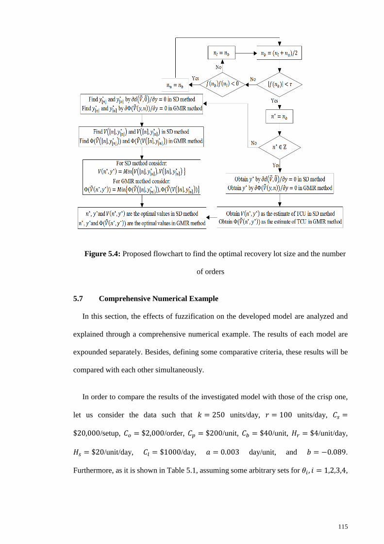
115

Figure 5.4: Proposed flowchart to find the optimal recovery lot size and the number

of orders

5.7 Comprehensive Numerical Example

In this section, the effects of fuzzification on the developed model are analyzed and

explained through a comprehensive numerical example. The results of each model are

expounded separately. Besides, defining some comparative criteria, these results will be

compared with each other simultaneously.

In order to compare the results of the investigated model with those of the crisp one,

let us consider the data such that 𝑘 = 250 units/day, 𝑟 = 100 units/day, 𝐶𝑠 =

$20,000/setup, 𝐶𝑜 = $2,000/order, 𝐶𝑝 = $200/unit, 𝐶𝑏 = $40/unit, 𝐻𝑟 = $4/unit/day,

𝐻𝑠 = $20/unit/day, 𝐶𝑙 = $1000/day, 𝑎 = 0.003 day/unit, and 𝑏 = −0.089.

Furthermore, as it is shown in Table 5.1, assuming some arbitrary sets for 𝜃𝑖 , 𝑖 = 1,2,3,4,

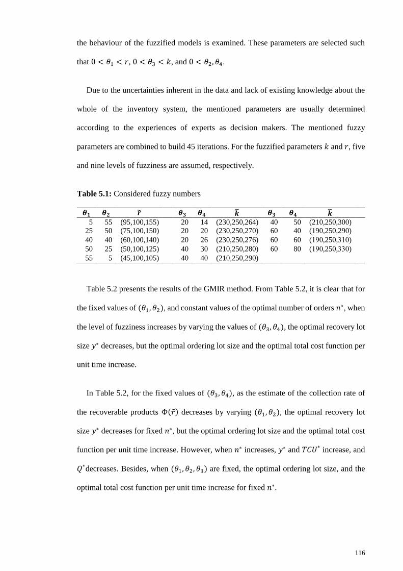
116

the behaviour of the fuzzified models is examined. These parameters are selected such

that 0 < 𝜃1 < 𝑟, 0 < 𝜃3 < 𝑘, and 0 < 𝜃2, 𝜃4.

Due to the uncertainties inherent in the data and lack of existing knowledge about the

whole of the inventory system, the mentioned parameters are usually determined

according to the experiences of experts as decision makers. The mentioned fuzzy

parameters are combined to build 45 iterations. For the fuzzified parameters 𝑘 and 𝑟, five

and nine levels of fuzziness are assumed, respectively.

Table 5.1: Considered fuzzy numbers

𝜽𝟏 𝜽𝟐 �̃� 𝜽𝟑 𝜽𝟒 �̃� 𝜽𝟑 𝜽𝟒 �̃�

5 55 (95,100,155) 20 14 (230,250,264) 40 50 (210,250,300)

25 50 (75,100,150) 20 20 (230,250,270) 60 40 (190,250,290) 40 40 (60,100,140) 20 26 (230,250,276) 60 60 (091,250,001) 50 25 (50,100,125) 40 30 (210,250,280) 60 80 (091,250,001) 55 5 (45,100,105) 40 40 (210,250,290)

Table 5.2 presents the results of the GMIR method. From Table 5.2, it is clear that for

the fixed values of (𝜃1, 𝜃2), and constant values of the optimal number of orders 𝑛∗, when

the level of fuzziness increases by varying the values of (𝜃3, 𝜃4), the optimal recovery lot

size 𝑦∗ decreases, but the optimal ordering lot size and the optimal total cost function per

unit time increase.

In Table 5.2, for the fixed values of (𝜃3, 𝜃4), as the estimate of the collection rate of

the recoverable products Φ(�̃�) decreases by varying (𝜃1, 𝜃2), the optimal recovery lot

size 𝑦∗ decreases for fixed 𝑛∗, but the optimal ordering lot size and the optimal total cost

function per unit time increase. However, when 𝑛∗ increases, 𝑦∗ and 𝑇𝐶𝑈∗ increase, and

𝑄∗decreases. Besides, when (𝜃1, 𝜃2, 𝜃3) are fixed, the optimal ordering lot size, and the

optimal total cost function per unit time increase for fixed 𝑛∗.

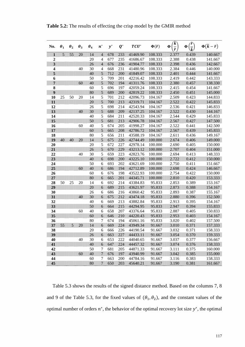
117

Table 5.2: The results of effecting the crisp model by the GMIR method

No. 𝜽𝟏 𝜽𝟐 𝜽𝟑 𝜽𝟒 𝒏∗ 𝒚∗ 𝑸∗ 𝑻𝑪𝑼∗ 𝚽(�̃�) 𝚽(�̃�

�̃�) 𝚽(

�̃�

�̃�) 𝚽(�̃� − �̃�)

1 5 55 20 14 4 678 233 41469.90 108.333 2.377 0.439 140.667

2 20 4 677 235 41686.67 108.333 2.388 0.438 141.667

3 26 4 676 236 41904.77 108.333 2.398 0.436 142.667

4 40 30 4 668 231 41480.96 108.333 2.384 0.446 140.000

5 40 5 712 200 41849.07 108.333 2.401 0.444 141.667

6 50 5 709 201 42216.42 108.333 2.419 0.442 143.333

7 60 40 5 702 194 41311.76 108.333 2.380 0.457 138.330

8 60 5 696 197 42059.24 108.333 2.415 0.454 141.667

9 80 5 689 200 42819.22 108.333 2.450 0.451 145.000

10 25 50 20 14 5 701 212 42096.73 104.167 2.509 0.423 144.833

11 20 5 700 213 42319.71 104.167 2.522 0.422 145.833

12 26 5 698 214 42543.94 104.167 2.536 0.421 146.833

13 40 30 5 688 209 42137.25 104.167 2.522 0.430 144.167

14 40 5 684 211 42520.33 104.167 2.544 0.429 145.833

15 50 5 681 213 42906.78 104.167 2.567 0.427 147.500

16 60 40 5 674 205 41998.27 104.167 2.522 0.441 142.500

17 60 5 665 208 42786.72 104.167 2.567 0.439 145.833

18 80 5 656 211 43588.19 104.167 2.611 0.436 149.167

19 40 40 20 14 5 675 226 42744.49 100.000 2.674 0.406 149.000

20 20 5 672 227 42978.14 100.000 2.690 0.405 150.000

21 26 5 670 229 43213.12 100.000 2.707 0.404 151.000

22 40 30 5 659 223 42823.76 100.000 2.694 0.413 148.333

23 40 6 698 200 43225.10 100.000 2.722 0.412 150.000

24 50 6 693 202 43621.69 100.000 2.750 0.411 151.667

25 60 40 6 686 194 42712.89 100.000 2.698 0.424 146.667

26 60 6 676 198 43522.93 100.000 2.754 0.422 150.000

27 80 6 665 201 44345.71 100.000 2.810 0.420 153.333

28 50 25 20 14 6 692 214 43384.83 95.833 2.853 0.389 153.167

29 20 6 689 215 43621.97 95.833 2.873 0.388 154.167

30 26 6 686 216 43860.42 95.833 2.893 0.387 155.167

31 40 30 6 675 212 43474.18 95.833 2.880 0.396 152.500

32 40 6 669 213 43882.84 95.833 2.913 0.395 154.167

33 50 6 664 215 44294.95 95.833 2.947 0.394 155.833

34 60 40 6 658 207 43376.64 95.833 2.887 0.405 150.833

35 60 6 646 210 44220.43 95.833 2.953 0.403 154.167

36 80 7 674 194 45061.16 95.833 3.020 0.402 157.500

37 55 5 20 14 6 669 224 43949.34 91.667 3.010 0.371 157.333

38 20 6 666 226 44190.54 91.667 3.032 0.371 158.333

39 26 6 663 227 44433.11 91.667 3.054 0.370 159.333

40 40 30 6 653 222 44040.65 91.667 3.037 0.377 156.667

41 40 6 647 224 44457.32 91.667 3.074 0.376 158.333

42 50 7 681 205 44871.33 91.667 3.111 0.375 160.000

43 60 40 7 676 197 43940.99 91.667 3.042 0.385 155.000

44 60 7 663 200 44784.16 91.667 3.116 0.383 158.333

45 80 7 650 203 45640.21 91.667 3.190 0.381 161.667

Table 5.3 shows the results of the signed distance method. Based on the columns 7, 8

and 9 of the Table 5.3, for the fixed values of (𝜃1, 𝜃2), and the constant values of the

optimal number of orders 𝑛∗, the behavior of the optimal recovery lot size 𝑦∗, the optimal

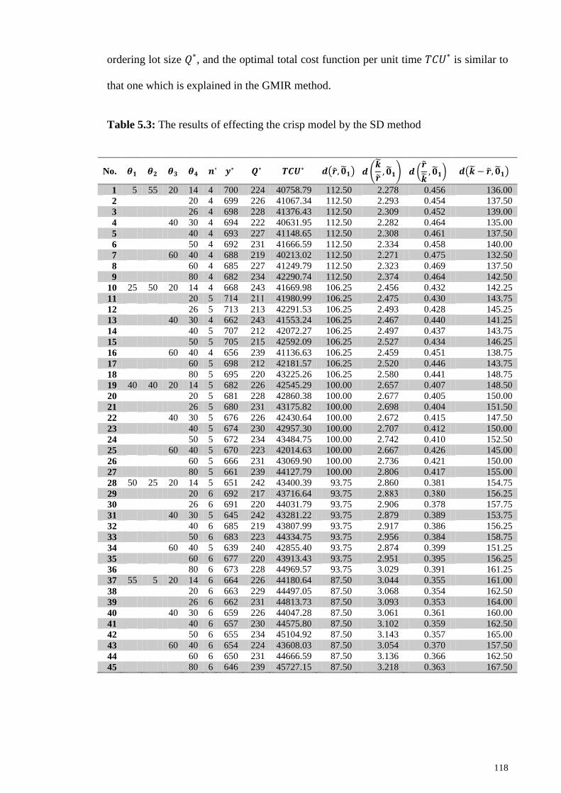
118

ordering lot size 𝑄∗, and the optimal total cost function per unit time 𝑇𝐶𝑈∗ is similar to

that one which is explained in the GMIR method.

Table 5.3: The results of effecting the crisp model by the SD method

No. 𝜽𝟏 𝜽𝟐 𝜽𝟑 𝜽𝟒 𝒏∗ 𝒚∗ 𝑸∗ 𝑻𝑪𝑼∗ 𝒅(�̃�, �̃�𝟏) 𝒅(�̃�

�̃�, �̃�𝟏) 𝒅 (

�̃�

�̃�, �̃�𝟏) 𝒅(�̃� − �̃�, �̃�𝟏)

1 5 55 20 14 4 700 224 40758.79 112.50 2.278 0.456 136.00

2 20 4 699 226 41067.34 112.50 2.293 0.454 137.50

3 26 4 698 228 41376.43 112.50 2.309 0.452 139.00

4 40 30 4 694 222 40631.95 112.50 2.282 0.464 135.00

5 40 4 693 227 41148.65 112.50 2.308 0.461 137.50

6 50 4 692 231 41666.59 112.50 2.334 0.458 140.00

7 60 40 4 688 219 40213.02 112.50 2.271 0.475 132.50

8 60 4 685 227 41249.79 112.50 2.323 0.469 137.50

9 80 4 682 234 42290.74 112.50 2.374 0.464 142.50

10 25 50 20 14 4 668 243 41669.98 106.25 2.456 0.432 142.25

11 20 5 407 200 41981.99 106.25 2.475 0.430 143.75

12 26 5 713 213 42291.53 106.25 2.493 0.428 145.25

13 40 30 4 662 243 41553.24 106.25 2.467 0.440 141.25

14 40 5 707 212 42072.27 106.25 2.497 0.437 143.75

15 50 5 705 215 42592.09 106.25 2.527 0.434 146.25

16 60 40 4 656 239 41136.63 106.25 2.459 0.451 138.75

17 60 5 698 212 42181.57 106.25 2.520 0.446 143.75

18 80 5 695 220 43225.26 106.25 2.580 0.441 148.75

19 40 40 20 14 5 682 226 42545.29 100.00 2.657 0.407 148.50

20 20 5 681 228 42860.38 100.00 2.677 0.405 150.00

21 26 5 680 231 43175.82 100.00 2.698 0.404 151.50

22 40 30 5 676 226 42430.64 100.00 2.672 0.415 147.50

23 40 5 674 230 42957.30 100.00 2.707 0.412 150.00

24 50 5 672 234 43484.75 100.00 2.742 0.410 152.50

25 60 40 5 670 223 42014.63 100.00 2.667 0.426 145.00

26 60 5 666 231 43069.90 100.00 2.736 0.421 150.00

27 80 5 661 239 44127.79 100.00 2.806 0.417 155.00

28 50 25 20 14 5 651 242 43400.39 93.75 2.860 0.381 154.75

29 20 6 692 217 43716.64 93.75 2.880 0.081 156.25

30 26 6 691 220 44031.79 93.75 2.906 0.378 157.75

31 40 30 5 645 242 43281.22 93.75 2.879 0.389 153.75

32 40 6 685 219 43807.99 93.75 2.917 0.386 156.25

33 50 6 683 223 44334.75 93.75 2.956 0.384 158.75

34 60 40 5 639 240 42855.40 93.75 2.874 0.399 151.25

35 60 6 677 220 43913.43 93.75 2.951 0.395 156.25

36 80 6 673 228 44969.57 93.75 3.029 0.391 161.25

37 55 5 20 14 6 664 226 44180.64 87.50 3.044 0.355 161.00

38 20 6 663 229 44497.05 87.50 3.068 0.354 162.50

39 26 6 662 231 44813.73 87.50 3.093 0.353 164.00

40 40 30 6 659 226 44047.28 87.50 3.061 0.361 160.00

41 40 6 657 230 44575.80 87.50 3.102 0.359 162.50

42 50 6 655 234 45104.92 87.50 3.143 0.357 165.00

43 60 40 6 654 224 43608.03 87.50 3.054 0.370 157.50

44 60 6 650 231 44666.59 87.50 3.136 0.366 162.50

45 80 6 646 239 45727.15 87.50 3.218 0.363 167.50

119

However, one of the major differences between them is that as 𝜃1 increases, the

decrease in 𝑦∗ is higher for the GMIR method as compared to the signed distance method.

Moreover, for the fixed values of (𝜃3, 𝜃4), as the estimate of the collection rate of the

recoverable products 𝑑(�̃�, 0̃1) decreases by varying (𝜃1, 𝜃2), the reduction in the optimal

recovery lot size 𝑦∗ is lower than that of the GMIR method for fixed 𝑛∗, and therewith,

the optimal ordering lot size 𝑄∗, and the optimal total cost function per unit time 𝑇𝐶𝑈∗

have the similar trends similar to the GMIR method.

The collection rate of the recoverable products from customers is an important factor

in the reverse logistics literature. For positive levels of fuzziness, the estimations of this

factor by the signed distance method are higher than those that are obtained applying the

GMIR method. Besides, it is observed that, for negative levels of fuzziness, the

estimations of the mentioned factor using the GMIR method returns higher value than the

signed distance method. These interesting results should be taken into consideration in

practical situations. In both methods, the optimal number of orders 𝑛∗ increases by

decreasing 𝜃2. In other words, the more the estimation of the difference between the

demand rate of the serviceable products and the collection rate of the recoverable products

(𝑘 − 𝑟), the higher the optimal number of orders 𝑛∗ will be.

Regarding a criterion defined in Eq. (5.49), the values of percentage changes for the

optimal recovery lot size 𝑄∗, and the optimal total cost function per unit time 𝑇𝐶𝑈∗

compared to the crisp ones are calculated in Table 5.4. For example, the 3th column of

Table 5.4 shows the percentage changes of optimal recovery lot size using the signed

distance method (𝑦𝑆𝐷∗ %).

(OptimalFuzzyValue − OptimalCrispValue

OptimalCrispValue) × 100 (5.49)

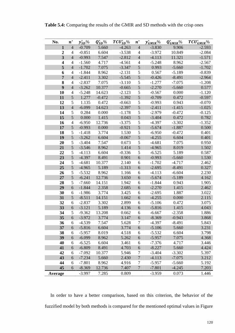
120

Table 5.4: Comparing the results of the GMIR and SD methods with the crisp ones

No. 𝒏∗ 𝒚𝑺𝑫∗ % 𝑸𝑺𝑫

∗ % 𝑻𝑪𝑼𝑺𝑫∗ % 𝒏∗ 𝒚𝑮𝑴𝑰𝑹

∗ % 𝑸𝑮𝑴𝑰𝑹∗ % 𝑻𝑪𝑼𝑮𝑴𝑰𝑹

∗ %

1 4 -0.709 5.660 -4.263 4 -3.830 9.906 -2.593

2 4 -0.851 6.604 -3.538 4 -3.972 10.849 -2.084

3 4 -0.993 7.547 -2.812 4 -4.113 11.321 -1.571

4 4 -1.560 4.717 -4.561 4 -5.248 8.962 -2.567

5 4 -1.702 7.075 -3.347 5 0.993 -5.660 -1.702

6 4 -1.844 8.962 -2.131 5 0.567 -5.189 -0.839

7 4 -2.411 3.302 -5.545 5 -0.426 -8.491 -2.964

8 4 -2.837 7.075 -3.110 5 -1.277 -7.075 -1.208

9 4 -3.262 10.377 -0.665 5 -2.270 -5.660 0.577

10 4 -5.248 14.623 -2.123 5 -0.567 0.000 -1.120

11 5 1.277 -0.472 -1.392 5 -0.709 0.472 -0.597

12 5 1.135 0.472 -0.663 5 -0.993 0.943 -0.070

13 4 -6.099 14.623 -2.397 5 -2.411 -1.415 -1.025

14 5 0.284 0.000 -1.178 5 -2.979 -0.472 -0.125

15 5 0.000 1.415 0.043 5 -3.404 0.472 0.782

16 4 -6.950 12.736 -3.375 5 -4.397 -3.302 -1.352

17 5 -0.993 0.000 -0.921 5 -5.674 -1.887 0.500

18 5 -1.418 3.774 1.530 5 -6.950 -0.472 0.401

19 5 -3.262 6.604 -0.067 5 -4.255 6.604 0.401

20 5 -3.404 7.547 0.673 5 -4.681 7.075 0.950

21 5 -3.546 8.962 1.414 5 -4.965 8.019 1.502

22 5 -4.113 6.604 -0.336 5 -6.525 5.189 0.587

23 5 -4.397 8.491 0.901 6 -0.993 -5.660 1.530

24 5 -4.681 10.377 2.140 6 -1.702 -4.717 2.462

25 5 -4.965 5.189 -1.313 6 -2.695 -8.491 0.327

26 5 -5.532 8.962 1.166 6 -4.113 -6.604 2.230

27 5 -6.241 12.736 3.650 6 -5.674 -5.189 4.162

28 5 -7.660 14.151 1.942 6 -1.844 0.943 1.905

29 6 -1.844 2.358 2.685 6 -2.270 1.415 2.462

30 6 -1.986 3.774 3.425 6 -2.695 1.887 3.022

31 5 -8.511 14.151 1.662 6 -4.255 0.000 2.115

32 6 -2.837 3.302 2.899 6 -5.106 0.472 3.075

33 6 -3.121 5.189 4.136 6 -5.816 1.415 4.043

34 5 -9.362 13.208 0.662 6 -6.667 -2.358 1.886

35 6 -3.972 3.774 3.147 6 -8.369 -0.943 3.868

36 6 -4.539 7.547 5.628 7 -4.397 -8.491 5.843

37 6 -5.816 6.604 3.774 6 -5.106 5.660 3.231

38 6 -5.957 8.019 4.518 6 -5.532 6.604 3.798

39 6 -6.099 8.962 5.262 6 -5.957 7.075 4.368

40 6 -6.525 6.604 3.461 6 -7.376 4.717 3.446

41 6 -6.809 8.491 4.703 6 -8.227 5.660 4.424

42 6 -7.092 10.377 5.946 7 -3.404 -3.302 5.397

43 6 -7.234 5.660 2.430 7 -4.113 -7.075 3.212

44 6 -7.801 8.962 4.916 7 -5.957 -5.660 5.192

45 6 -8.369 12.736 7.407 7 -7.801 -4.245 7.203

Average -3.997 7.285 0.809 -3.959 0.073 1.446

In order to have a better comparison, based on this criterion, the behavior of the

fuzzified model by both methods is compared for the mentioned optimal values in Figure

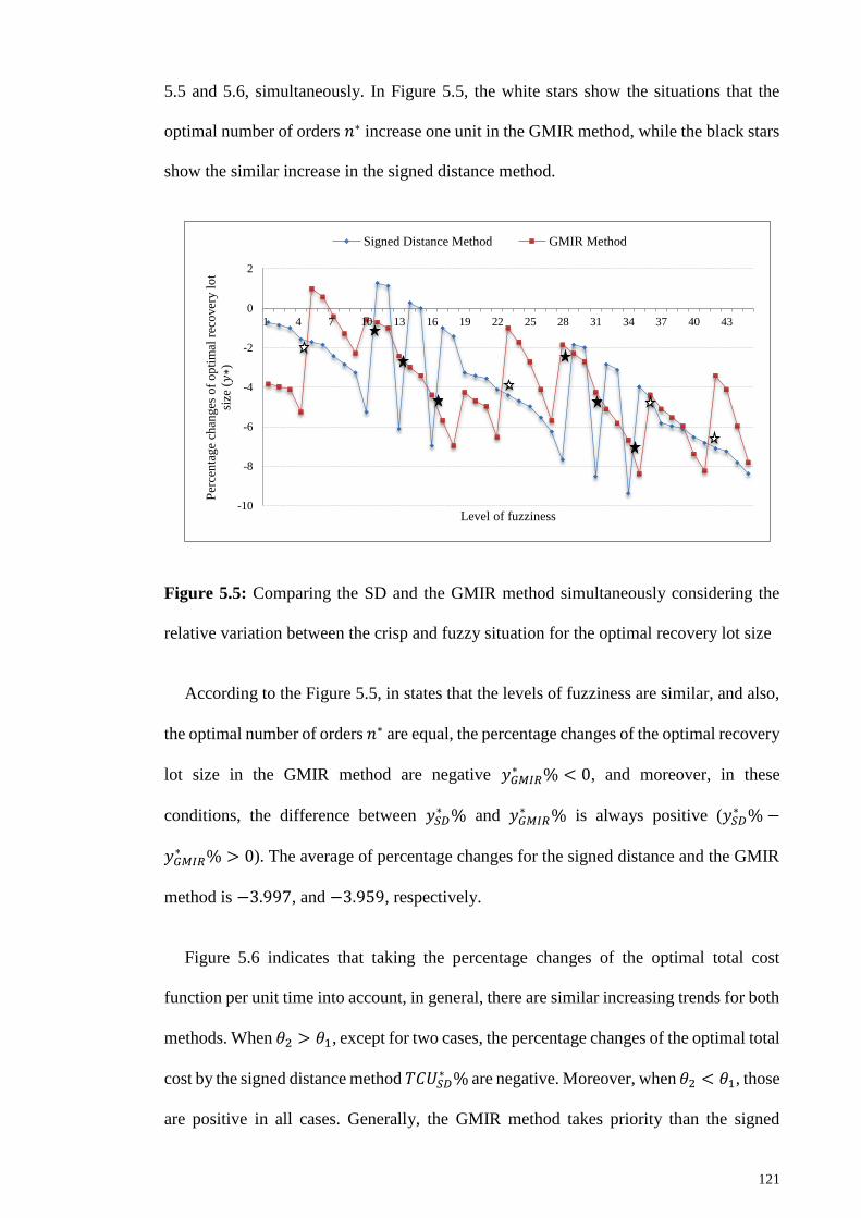
121

5.5 and 5.6, simultaneously. In Figure 5.5, the white stars show the situations that the

optimal number of orders 𝑛∗ increase one unit in the GMIR method, while the black stars

show the similar increase in the signed distance method.


relative variation between the crisp and fuzzy situation for the optimal recovery lot size

According to the Figure 5.5, in states that the levels of fuzziness are similar, and also,

the optimal number of orders 𝑛∗ are equal, the percentage changes of the optimal recovery

lot size in the GMIR method are negative 𝑦𝐺𝑀𝐼𝑅∗ % < 0, and moreover, in these

conditions, the difference between 𝑦𝑆𝐷∗ % and 𝑦𝐺𝑀𝐼𝑅

∗ % is always positive (𝑦𝑆𝐷∗ %−

𝑦𝐺𝑀𝐼𝑅∗ % > 0). The average of percentage changes for the signed distance and the GMIR

method is −3.997, and −3.959, respectively.

Figure 5.6 indicates that taking the percentage changes of the optimal total cost

function per unit time into account, in general, there are similar increasing trends for both

methods. When 𝜃2 > 𝜃1, except for two cases, the percentage changes of the optimal total

cost by the signed distance method 𝑇𝐶𝑈𝑆𝐷∗ % are negative. Moreover, when 𝜃2 < 𝜃1, those

are positive in all cases. Generally, the GMIR method takes priority than the signed

-10

-8

-6

-4

-2

0

2

1 4 7 10 13 16 19 22 25 28 31 34 37 40 43

Per

cen

tage

chan

ges

of

op

tim

al r

eco

ver

y l

ot

size

(𝑦∗)

Level of fuzziness

Signed Distance Method GMIR Method

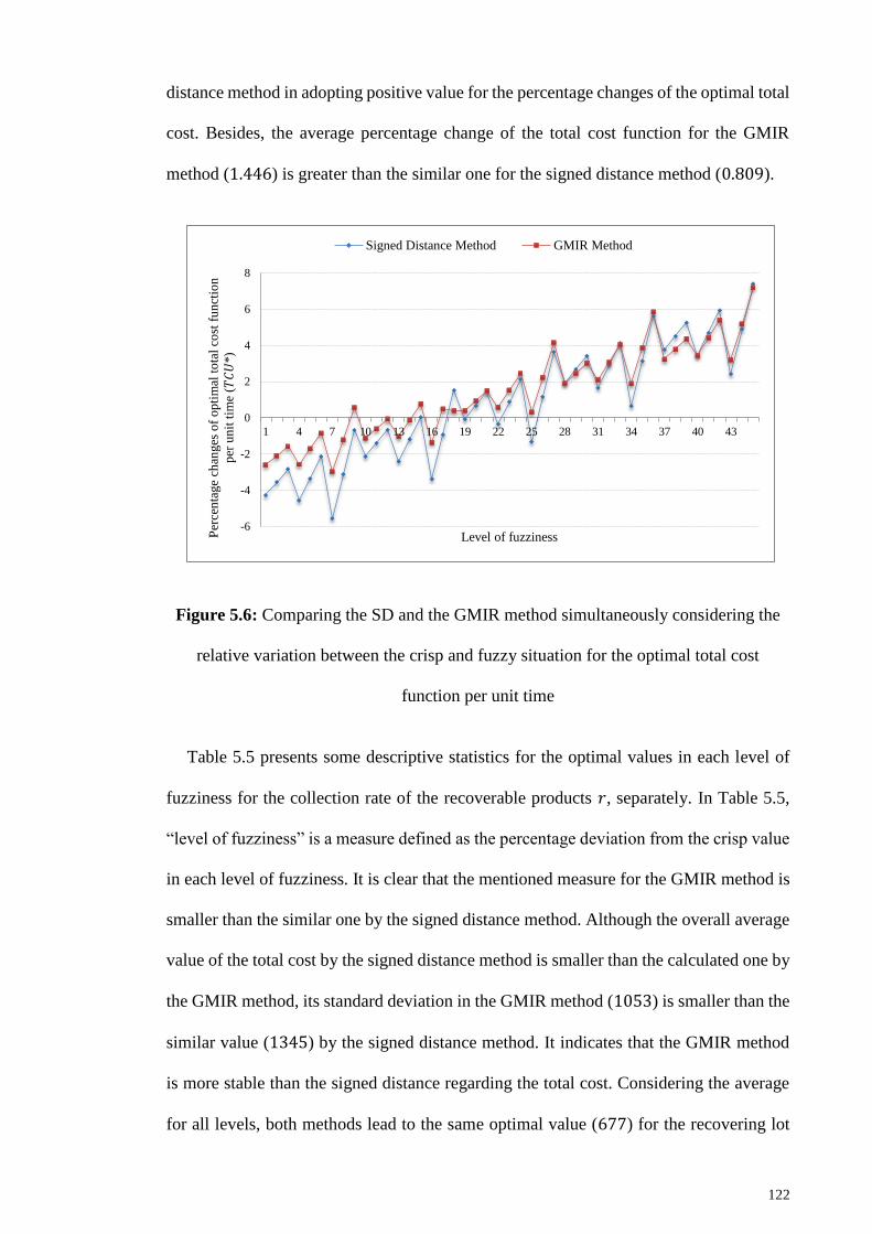
122

distance method in adopting positive value for the percentage changes of the optimal total

cost. Besides, the average percentage change of the total cost function for the GMIR

method (1.446) is greater than the similar one for the signed distance method (0.809).


relative variation between the crisp and fuzzy situation for the optimal total cost

function per unit time

Table 5.5 presents some descriptive statistics for the optimal values in each level of

fuzziness for the collection rate of the recoverable products 𝑟, separately. In Table 5.5,

“level of fuzziness” is a measure defined as the percentage deviation from the crisp value

in each level of fuzziness. It is clear that the mentioned measure for the GMIR method is

smaller than the similar one by the signed distance method. Although the overall average

value of the total cost by the signed distance method is smaller than the calculated one by

the GMIR method, its standard deviation in the GMIR method (1053) is smaller than the

similar value (1345) by the signed distance method. It indicates that the GMIR method

is more stable than the signed distance regarding the total cost. Considering the average

for all levels, both methods lead to the same optimal value (677) for the recovering lot

-6

-4

-2

0

2

4

6

8

1 4 7 10 13 16 19 22 25 28 31 34 37 40 43

Per

cen

tage

chan

ges

of

op

tim

al t

ota

l co

st f

un

ctio

n

per

un

it t

ime

(𝑇𝐶𝑈

*)

Level of fuzziness

Signed Distance Method GMIR Method

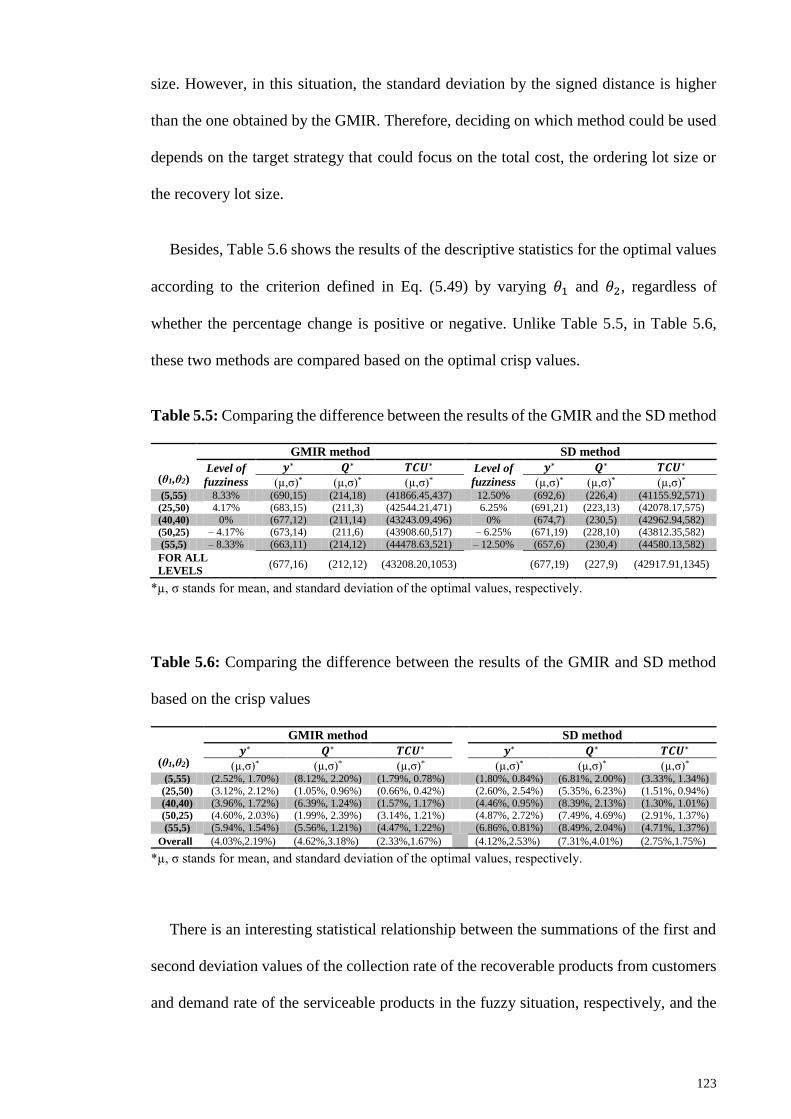
123

size. However, in this situation, the standard deviation by the signed distance is higher

than the one obtained by the GMIR. Therefore, deciding on which method could be used

depends on the target strategy that could focus on the total cost, the ordering lot size or

the recovery lot size.

Besides, Table 5.6 shows the results of the descriptive statistics for the optimal values

according to the criterion defined in Eq. (5.49) by varying 𝜃1 and 𝜃2, regardless of

whether the percentage change is positive or negative. Unlike Table 5.5, in Table 5.6,

these two methods are compared based on the optimal crisp values.

Table 5.5: Comparing the difference between the results of the GMIR and the SD method

(θ1,θ2)

GMIR method SD method

Level of

fuzziness

𝒚∗ 𝑸∗ 𝑻𝑪𝑼∗ Level of

fuzziness

𝒚∗ 𝑸∗ 𝑻𝑪𝑼∗

(µ,σ)* (µ,σ)* (µ,σ)* (µ,σ)* (µ,σ)* (µ,σ)* (5,55) 8.33% (690,15) (214,18) (41866.45,437) 12.50% (692,6) (226,4) (41155.92,571)

(25,50) 4.17% (683,15) (211,3) (42544.21,471) 6.25% (691,21) (223,13) (42078.17,575)

(40,40) 0% (677,12) (211,14) (43243.09,496) 0% (674,7) (230,5) (42962.94,582)

(50,25) ‒ 4.17% (673,14) (211,6) (43908.60,517) ‒ 6.25% (671,19) (228,10) (43812.35,582)

(55,5) ‒ 8.33% (663,11) (214,12) (44478.63,521) ‒ 12.50% (657,6) (230,4) (44580.13,582)

FOR ALL

LEVELS (677,16) (212,12) (43208.20,1053) (677,19) (227,9) (42917.91,1345)

*µ, σ stands for mean, and standard deviation of the optimal values, respectively.

Table 5.6: Comparing the difference between the results of the GMIR and SD method

based on the crisp values

(θ1,θ2)

GMIR method SD method 𝒚∗ 𝑸∗ 𝑻𝑪𝑼∗ 𝒚∗ 𝑸∗ 𝑻𝑪𝑼∗

(µ,σ)* (µ,σ)* (µ,σ)* (µ,σ)* (µ,σ)* (µ,σ)* (5,55) (2.52%, 1.70%) (8.12%, 2.20%) (1.79%, 0.78%) (1.80%, 0.84%) (6.81%, 2.00%) (3.33%, 1.34%)

(25,50) (3.12%, 2.12%) (1.05%, 0.96%) (0.66%, 0.42%) (2.60%, 2.54%) (5.35%, 6.23%) (1.51%, 0.94%)

(40,40) (3.96%, 1.72%) (6.39%, 1.24%) (1.57%, 1.17%) (4.46%, 0.95%) (8.39%, 2.13%) (1.30%, 1.01%)

(50,25) (4.60%, 2.03%) (1.99%, 2.39%) (3.14%, 1.21%) (4.87%, 2.72%) (7.49%, 4.69%) (2.91%, 1.37%)

(55,5) (5.94%, 1.54%) (5.56%, 1.21%) (4.47%, 1.22%) (6.86%, 0.81%) (8.49%, 2.04%) (4.71%, 1.37%)

Overall (4.03%,2.19%) (4.62%,3.18%) (2.33%,1.67%) (4.12%,2.53%) (7.31%,4.01%) (2.75%,1.75%)

*µ, σ stands for mean, and standard deviation of the optimal values, respectively.

There is an interesting statistical relationship between the summations of the first and

second deviation values of the collection rate of the recoverable products from customers

and demand rate of the serviceable products in the fuzzy situation, respectively, and the

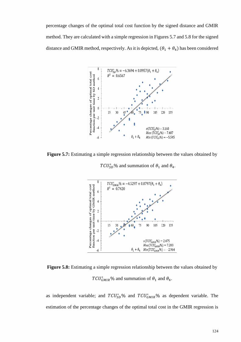
124

percentage changes of the optimal total cost function by the signed distance and GMIR

method. They are calculated with a simple regression in Figures 5.7 and 5.8 for the signed

distance and GMIR method, respectively. As it is depicted, (𝜃1 + 𝜃4) has been considered


𝑇𝐶𝑈𝑆𝐷∗ % and summation of 𝜃1 and 𝜃4.


𝑇𝐶𝑈𝐺𝑀𝐼𝑅∗ % and summation of 𝜃1 and 𝜃4.

as independent variable; and 𝑇𝐶𝑈𝑆𝐷∗ % and 𝑇𝐶𝑈𝐺𝑀𝐼𝑅

∗ % as dependent variable. The

estimation of the percentage changes of the optimal total cost in the GMIR regression is

125

about 10 percent better than the one obtained by signed distance regression because the

value of R-square in the first one is about 10 units greater than the second one.

5.8 Chapter Summary

One of the most important issues in the reverse inventory models is the lack of

historical data for the demand and return (collection) rate. Accordingly, estimation of the

probability distributions of such parameters is not possible. Therefore, these parameters

are not determined, and usually it is not logical to decide based on the crisp values while

the situation is uncertain. With these perspectives, it is worthwhile to reconsider the

reverse inventory system with the learning effect (Tsai, 2012) and provide an alternative

approach.

In this chapter, two fuzzy models were proposed for a reverse inventory problem with

the learning effect. In both models, the demand rate of the serviceable products and the

collection rate of the recoverable products from customers were presented as fuzzy

numbers. To estimate the total cost function per unit time in the fuzzy sense, and then the

corresponding optimal recovery lot size and the number of orders for the newly purchased

products, in the first model, the signed distance method was employed for the

defuzzification, while the GMIR was used in the second one. These models were

explained and solved by a comprehensive numerical example. The results of both are

compared methods. Besides, it is concluded that it is important to decide which method

should be chosen regarding the considered strategies.

It is noteworthy that although there are some researches in the forward supply chain

literature, which considered fuzzy EOQ/EPQ, there is no similar work in the reverse

supply chain literature that compares the performance of the well-known defuzzification

methods such as the GMIR and the signed distance method. In this study, the performance

126

of the mentioned methods is compared in the presence of learning in a reverse inventory

model.

127

CHAPTER 6: APPLICATIONS TO CASE STUDIES

6.1 Introduction

In this chapter, the application of the previous developed fuzzy inventory models is

introduced through real case studies. However, usually it is difficult to match the

theoretical models to the real world scenario completely. Because there are many

uncontrollable factors in the business environment that influence the whole of the

inventory system.

The first fuzzy model introduced in chapter four is tried to be explained via a case from

an automobile industry, and later, the second one suggested in chapter five is discussed

through a milk manufacturing company. The most important focus of this chapter is to

show that these fuzzy models can improve the policies for decision makers and managers

in organization.

6.2 First Case Study

The first case is related to a supply chain network in an automobile industry where

there is a supplier and manufacturer who produces some parts of a special automobile to

sell to the other manufacturers. Firstly, the manufacturer and the supplier are introduced

and the relation of the whole supply chain is depicted.

6.2.1 A Supply Chain in an Automobile Industry

The manufacturer that is studied here is a company called Auto Chassis International

Pars (ACI Pars) belonged to the supply chain network of Groupe Renault International in

Tehran, Iran. This company is established in 2005 incorporating Robat Machine Co. and

Renault by a joint venture as 23% and 77% stock respectively. The company produces

and assembles automobile parts specially chassis systems and components of L-90

(Tondar 90) and U-90 products. Figure 6.1 shows a sample of produced L-90.

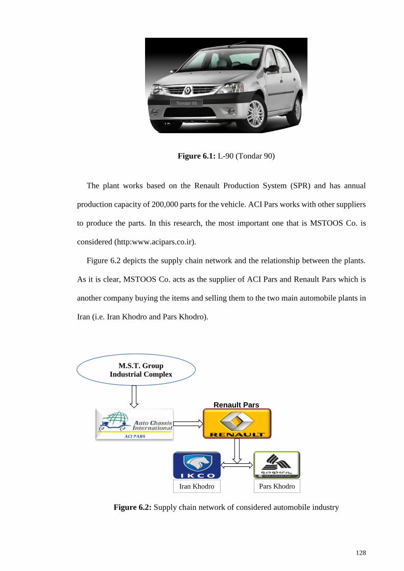
128

Figure 6.1: L-90 (Tondar 90)

The plant works based on the Renault Production System (SPR) and has annual

production capacity of 200,000 parts for the vehicle. ACI Pars works with other suppliers

to produce the parts. In this research, the most important one that is MSTOOS Co. is

considered (http:www.acipars.co.ir).

Figure 6.2 depicts the supply chain network and the relationship between the plants.

As it is clear, MSTOOS Co. acts as the supplier of ACI Pars and Renault Pars which is

another company buying the items and selling them to the two main automobile plants in

Iran (i.e. Iran Khodro and Pars Khodro).

Figure 6.2: Supply chain network of considered automobile industry

M.S.T. Group

Industrial Complex

Renault Pars

Iran Khodro Pars Khodro

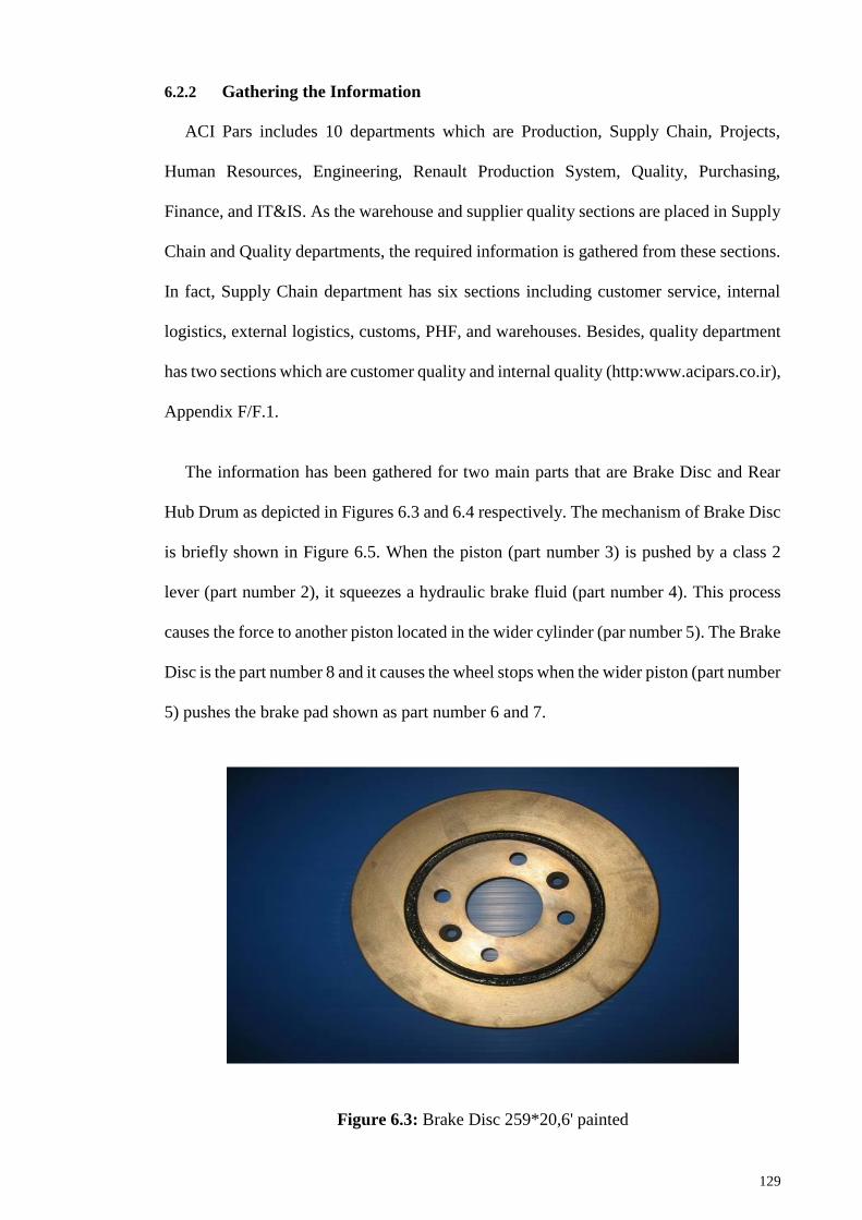
129

6.2.2 Gathering the Information

ACI Pars includes 10 departments which are Production, Supply Chain, Projects,

Human Resources, Engineering, Renault Production System, Quality, Purchasing,

Finance, and IT&IS. As the warehouse and supplier quality sections are placed in Supply

Chain and Quality departments, the required information is gathered from these sections.

In fact, Supply Chain department has six sections including customer service, internal

logistics, external logistics, customs, PHF, and warehouses. Besides, quality department

has two sections which are customer quality and internal quality (http:www.acipars.co.ir),

Appendix F/F.1.

The information has been gathered for two main parts that are Brake Disc and Rear

Hub Drum as depicted in Figures 6.3 and 6.4 respectively. The mechanism of Brake Disc

is briefly shown in Figure 6.5. When the piston (part number 3) is pushed by a class 2

lever (part number 2), it squeezes a hydraulic brake fluid (part number 4). This process

causes the force to another piston located in the wider cylinder (par number 5). The Brake

Disc is the part number 8 and it causes the wheel stops when the wider piston (part number

5) pushes the brake pad shown as part number 6 and 7.

Figure 6.3: Brake Disc 259*20,6' painted

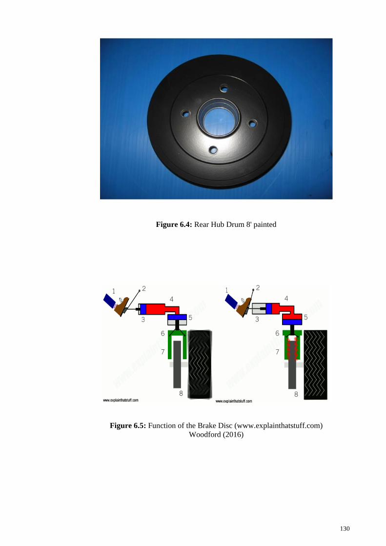
130

Figure 6.4: Rear Hub Drum 8' painted

Figure 6.5: Function of the Brake Disc (www.explainthatstuff.com)

Woodford (2016)

http://www.explainthatstuff.com/

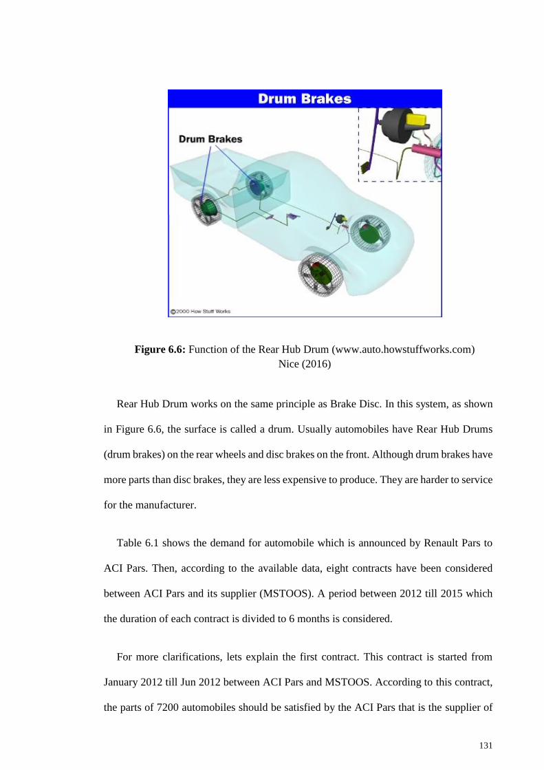
131

Figure 6.6: Function of the Rear Hub Drum (www.auto.howstuffworks.com)

Nice (2016)

Rear Hub Drum works on the same principle as Brake Disc. In this system, as shown

in Figure 6.6, the surface is called a drum. Usually automobiles have Rear Hub Drums

(drum brakes) on the rear wheels and disc brakes on the front. Although drum brakes have

more parts than disc brakes, they are less expensive to produce. They are harder to service

for the manufacturer.

Table 6.1 shows the demand for automobile which is announced by Renault Pars to

ACI Pars. Then, according to the available data, eight contracts have been considered

between ACI Pars and its supplier (MSTOOS). A period between 2012 till 2015 which

the duration of each contract is divided to 6 months is considered.

For more clarifications, lets explain the first contract. This contract is started from

January 2012 till Jun 2012 between ACI Pars and MSTOOS. According to this contract,

the parts of 7200 automobiles should be satisfied by the ACI Pars that is the supplier of

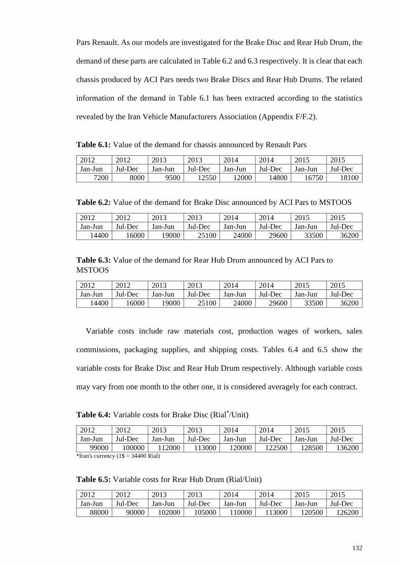
132

Pars Renault. As our models are investigated for the Brake Disc and Rear Hub Drum, the

demand of these parts are calculated in Table 6.2 and 6.3 respectively. It is clear that each

chassis produced by ACI Pars needs two Brake Discs and Rear Hub Drums. The related

information of the demand in Table 6.1 has been extracted according to the statistics

revealed by the Iran Vehicle Manufacturers Association (Appendix F/F.2).

Table 6.1: Value of the demand for chassis announced by Renault Pars

2012 2012 2013 2013 2014 2014 2015 2015

Jan-Jun Jul-Dec Jan-Jun Jul-Dec Jan-Jun Jul-Dec Jan-Jun Jul-Dec

7200 8000 9500 12550 12000 14800 16750 18100

Table 6.2: Value of the demand for Brake Disc announced by ACI Pars to MSTOOS

2012 2012 2013 2013 2014 2014 2015 2015


14400 16000 19000 25100 24000 29600 33500 36200

Table 6.3: Value of the demand for Rear Hub Drum announced by ACI Pars to

MSTOOS

2012 2012 2013 2013 2014 2014 2015 2015


14400 16000 19000 25100 24000 29600 33500 36200

Variable costs include raw materials cost, production wages of workers, sales

commissions, packaging supplies, and shipping costs. Tables 6.4 and 6.5 show the

variable costs for Brake Disc and Rear Hub Drum respectively. Although variable costs

may vary from one month to the other one, it is considered averagely for each contract.

Table 6.4: Variable costs for Brake Disc (Rial*/Unit)

2012 2012 2013 2013 2014 2014 2015 2015


99000 100000 112000 113000 120000 122500 128500 136200 *Iran's currency (1$ ≈ 34400 Rial)

Table 6.5: Variable costs for Rear Hub Drum (Rial/Unit)

2012 2012 2013 2013 2014 2014 2015 2015


88000 90000 102000 105000 110000 113000 120500 126200

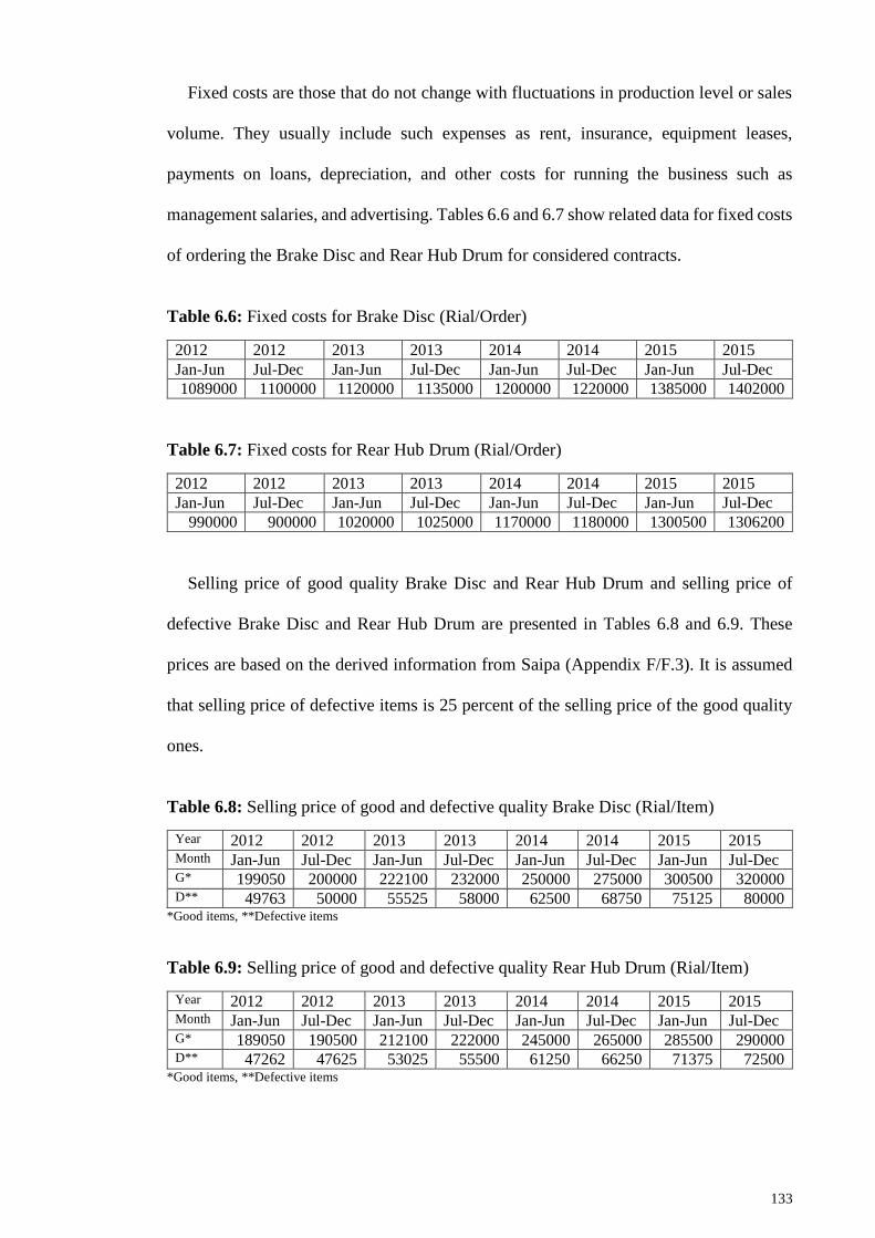
133

Fixed costs are those that do not change with fluctuations in production level or sales

volume. They usually include such expenses as rent, insurance, equipment leases,

payments on loans, depreciation, and other costs for running the business such as

management salaries, and advertising. Tables 6.6 and 6.7 show related data for fixed costs

of ordering the Brake Disc and Rear Hub Drum for considered contracts.

Table 6.6: Fixed costs for Brake Disc (Rial/Order)

2012 2012 2013 2013 2014 2014 2015 2015


1089000 1100000 1120000 1135000 1200000 1220000 1385000 1402000

Table 6.7: Fixed costs for Rear Hub Drum (Rial/Order)

2012 2012 2013 2013 2014 2014 2015 2015


990000 900000 1020000 1025000 1170000 1180000 1300500 1306200

Selling price of good quality Brake Disc and Rear Hub Drum and selling price of

defective Brake Disc and Rear Hub Drum are presented in Tables 6.8 and 6.9. These

prices are based on the derived information from Saipa (Appendix F/F.3). It is assumed

that selling price of defective items is 25 percent of the selling price of the good quality

ones.

Table 6.8: Selling price of good and defective quality Brake Disc (Rial/Item)

Year 2012 2012 2013 2013 2014 2014 2015 2015 Month Jan-Jun Jul-Dec Jan-Jun Jul-Dec Jan-Jun Jul-Dec Jan-Jun Jul-Dec G* 199050 200000 222100 232000 250000 275000 300500 320000 D** 49763 50000 55525 58000 62500 68750 75125 80000

*Good items, **Defective items

Table 6.9: Selling price of good and defective quality Rear Hub Drum (Rial/Item)

Year 2012 2012 2013 2013 2014 2014 2015 2015 Month Jan-Jun Jul-Dec Jan-Jun Jul-Dec Jan-Jun Jul-Dec Jan-Jun Jul-Dec G* 189050 190500 212100 222000 245000 265000 285500 290000 D** 47262 47625 53025 55500 61250 66250 71375 72500

*Good items, **Defective items

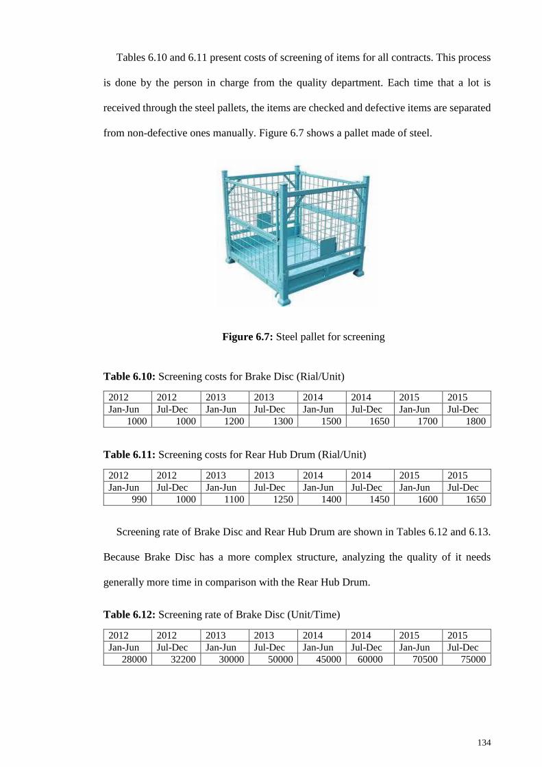
134

Tables 6.10 and 6.11 present costs of screening of items for all contracts. This process

is done by the person in charge from the quality department. Each time that a lot is

received through the steel pallets, the items are checked and defective items are separated

from non-defective ones manually. Figure 6.7 shows a pallet made of steel.

Figure 6.7: Steel pallet for screening

Table 6.10: Screening costs for Brake Disc (Rial/Unit)

2012 2012 2013 2013 2014 2014 2015 2015


1000 1000 1200 1300 1500 1650 1700 1800

Table 6.11: Screening costs for Rear Hub Drum (Rial/Unit)

2012 2012 2013 2013 2014 2014 2015 2015


990 1000 1100 1250 1400 1450 1600 1650

Screening rate of Brake Disc and Rear Hub Drum are shown in Tables 6.12 and 6.13.

Because Brake Disc has a more complex structure, analyzing the quality of it needs

generally more time in comparison with the Rear Hub Drum.

Table 6.12: Screening rate of Brake Disc (Unit/Time)

2012 2012 2013 2013 2014 2014 2015 2015


28000 32200 30000 50000 45000 60000 70500 75000

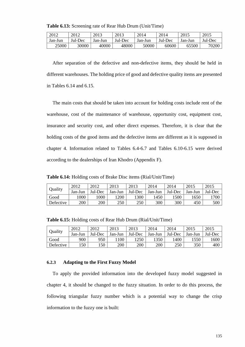
135

Table 6.13: Screening rate of Rear Hub Drum (Unit/Time)

2012 2012 2013 2013 2014 2014 2015 2015


25000 30000 40000 48000 50000 60600 65500 70200

After separation of the defective and non-defective items, they should be held in

different warehouses. The holding price of good and defective quality items are presented

in Tables 6.14 and 6.15.

The main costs that should be taken into account for holding costs include rent of the

warehouse, cost of the maintenance of warehouse, opportunity cost, equipment cost,

insurance and security cost, and other direct expenses. Therefore, it is clear that the

holding costs of the good items and the defective items are different as it is supposed in

chapter 4. Information related to Tables 6.4-6.7 and Tables 6.10-6.15 were derived

according to the dealerships of Iran Khodro (Appendix F).

Table 6.14: Holding costs of Brake Disc items (Rial/Unit/Time)

Quality 2012 2012 2013 2013 2014 2014 2015 2015


Good 1000 1000 1200 1300 1450 1500 1650 1700

Defective 200 200 250 250 300 300 450 500

Table 6.15: Holding costs of Rear Hub Drum (Rial/Unit/Time)

Quality 2012 2012 2013 2013 2014 2014 2015 2015


Good 900 950 1100 1250 1350 1400 1550 1600

Defective 150 150 200 200 200 250 350 400

6.2.3 Adapting to the First Fuzzy Model

To apply the provided information into the developed fuzzy model suggested in

chapter 4, it should be changed to the fuzzy situation. In order to do this process, the

following triangular fuzzy number which is a potential way to change the crisp

information to the fuzzy one is built:

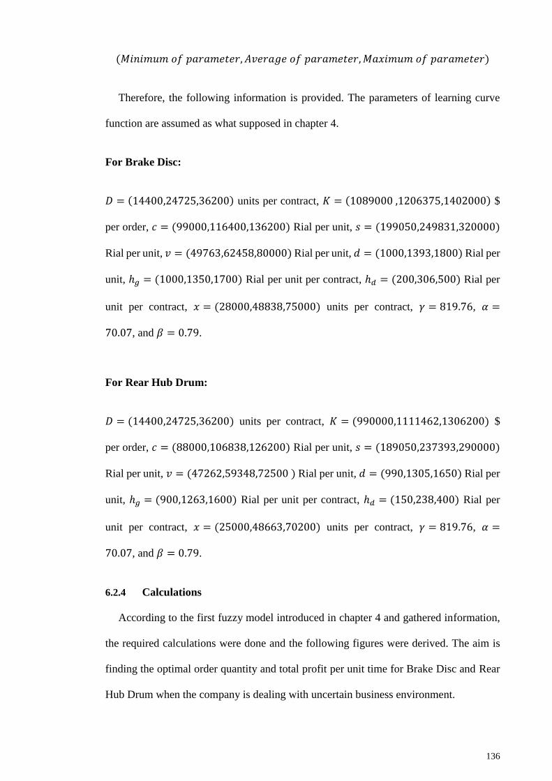
136

(𝑀𝑖𝑛𝑖𝑚𝑢𝑚𝑜𝑓𝑝𝑎𝑟𝑎𝑚𝑒𝑡𝑒𝑟, 𝐴𝑣𝑒𝑟𝑎𝑔𝑒𝑜𝑓𝑝𝑎𝑟𝑎𝑚𝑒𝑡𝑒𝑟,𝑀𝑎𝑥𝑖𝑚𝑢𝑚𝑜𝑓𝑝𝑎𝑟𝑎𝑚𝑒𝑡𝑒𝑟)

Therefore, the following information is provided. The parameters of learning curve

function are assumed as what supposed in chapter 4.

For Brake Disc:

𝐷 = (14400,24725,36200) units per contract, 𝐾 = (1089000,1206375,1402000) $

per order, 𝑐 = (99000,116400,136200) Rial per unit, 𝑠 = (199050,249831,320000)

Rial per unit, 𝑣 = (49763,62458,80000) Rial per unit, 𝑑 = (1000,1393,1800) Rial per

unit, ℎ𝑔 = (1000,1350,1700) Rial per unit per contract, ℎ𝑑 = (200,306,500) Rial per

unit per contract, 𝑥 = (28000,48838,75000) units per contract, 𝛾 = 819.76, 𝛼 =

70.07, and 𝛽 = 0.79.

For Rear Hub Drum:

𝐷 = (14400,24725,36200) units per contract, 𝐾 = (990000,1111462,1306200) $

per order, 𝑐 = (88000,106838,126200) Rial per unit, 𝑠 = (189050,237393,290000)

Rial per unit, 𝑣 = (47262,59348,72500) Rial per unit, 𝑑 = (990,1305,1650) Rial per

unit, ℎ𝑔 = (900,1263,1600) Rial per unit per contract, ℎ𝑑 = (150,238,400) Rial per

unit per contract, 𝑥 = (25000,48663,70200) units per contract, 𝛾 = 819.76, 𝛼 =

70.07, and 𝛽 = 0.79.

6.2.4 Calculations

According to the first fuzzy model introduced in chapter 4 and gathered information,

the required calculations were done and the following figures were derived. The aim is

finding the optimal order quantity and total profit per unit time for Brake Disc and Rear

Hub Drum when the company is dealing with uncertain business environment.

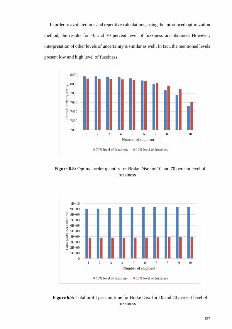
137

In order to avoid tedious and repetitive calculations, using the introduced optimization

method, the results for 10 and 70 percent level of fuzziness are obtained. However,

interpretation of other levels of uncertainty is similar as well. In fact, the mentioned levels

present low and high level of fuzziness.

Figure 6.8: Optimal order quantity for Brake Disc for 10 and 70 percent level of

fuzziness

Figure 6.9: Total profit per unit time for Brake Disc for 10 and 70 percent level of

fuzziness

7050

7250

7450

7650

7850

8050

8250

1 2 3 4 5 6 7 8 9 10

Op

tim

al o

rder

quan

tity

Number of shipment

70% level of fuzziness 10% level of fuzziness

0

1E+09

2E+09

3E+09

4E+09

5E+09

6E+09

7E+09

8E+09

9E+09

1E+10

1 2 3 4 5 6 7 8 9 10

To

tal

pro

fit

per

unit

tim

e

Number of shipment


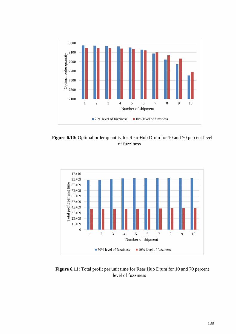
138

Figure 6.10: Optimal order quantity for Rear Hub Drum for 10 and 70 percent level

of fuzziness

Figure 6.11: Total profit per unit time for Rear Hub Drum for 10 and 70 percent

level of fuzziness

7100

7300

7500

7700

7900

8100

8300

1 2 3 4 5 6 7 8 9 10

Op

tim

al o

rder

quan

tity

Number of shipment


0

1E+09

2E+09

3E+09

4E+09

5E+09

6E+09

7E+09

8E+09

9E+09

1E+10

1 2 3 4 5 6 7 8 9 10

To

tal

pro

fit

per

unit

tim

e

Number of shipment


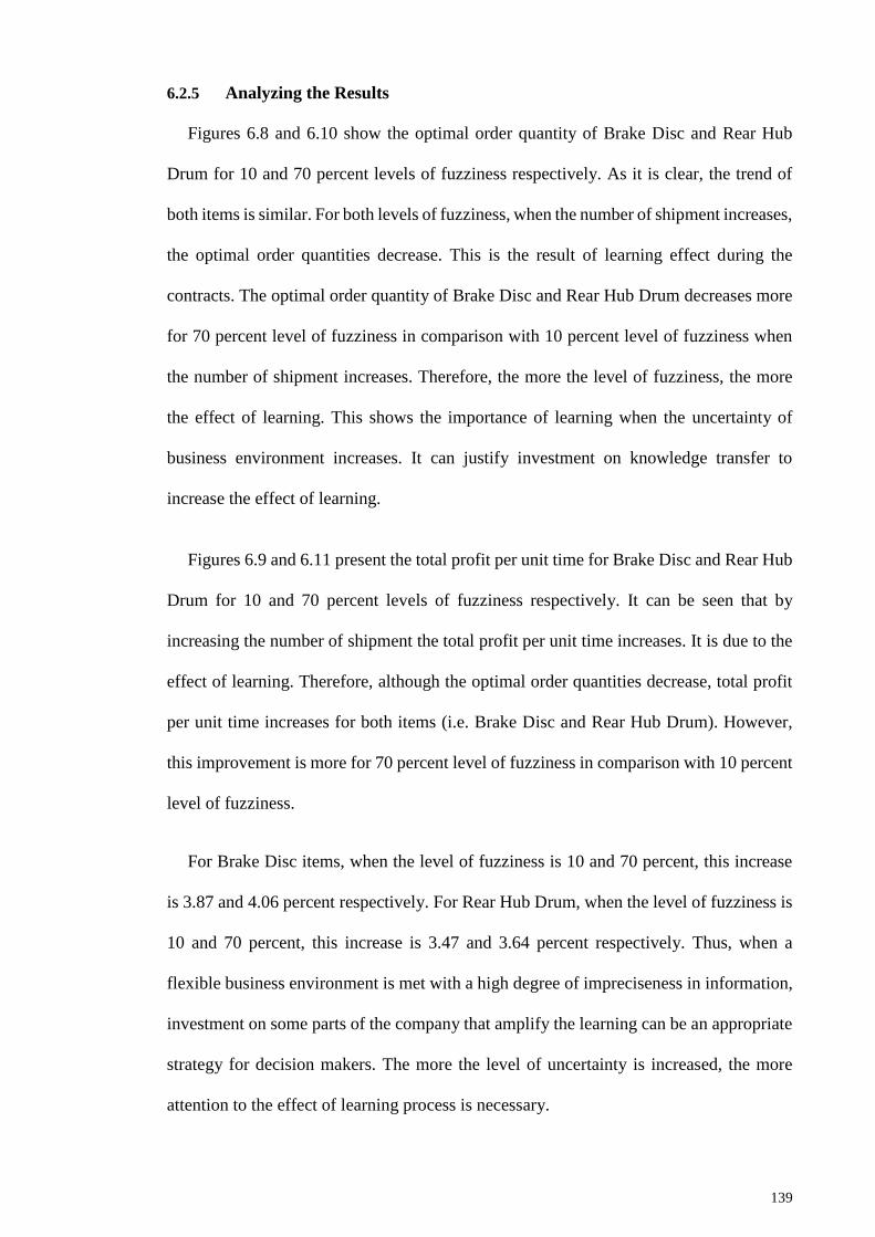
139

6.2.5 Analyzing the Results

Figures 6.8 and 6.10 show the optimal order quantity of Brake Disc and Rear Hub

Drum for 10 and 70 percent levels of fuzziness respectively. As it is clear, the trend of

both items is similar. For both levels of fuzziness, when the number of shipment increases,

the optimal order quantities decrease. This is the result of learning effect during the

contracts. The optimal order quantity of Brake Disc and Rear Hub Drum decreases more

for 70 percent level of fuzziness in comparison with 10 percent level of fuzziness when

the number of shipment increases. Therefore, the more the level of fuzziness, the more

the effect of learning. This shows the importance of learning when the uncertainty of

business environment increases. It can justify investment on knowledge transfer to

increase the effect of learning.

Figures 6.9 and 6.11 present the total profit per unit time for Brake Disc and Rear Hub

Drum for 10 and 70 percent levels of fuzziness respectively. It can be seen that by

increasing the number of shipment the total profit per unit time increases. It is due to the

effect of learning. Therefore, although the optimal order quantities decrease, total profit

per unit time increases for both items (i.e. Brake Disc and Rear Hub Drum). However,

this improvement is more for 70 percent level of fuzziness in comparison with 10 percent

level of fuzziness.

For Brake Disc items, when the level of fuzziness is 10 and 70 percent, this increase

is 3.87 and 4.06 percent respectively. For Rear Hub Drum, when the level of fuzziness is

10 and 70 percent, this increase is 3.47 and 3.64 percent respectively. Thus, when a

flexible business environment is met with a high degree of impreciseness in information,

investment on some parts of the company that amplify the learning can be an appropriate

strategy for decision makers. The more the level of uncertainty is increased, the more

attention to the effect of learning process is necessary.

140

6.3 Second Case Study

The second case study is related to the application of the second fuzzy model

introduced in chapter five through the milk industry. At first, let’s introduce the

companies and explain their activities.

6.3.1 Milk Manufacturing Company

In this section, the activity of the factories that are included in our second case study

is explained and is briefly introduced. However, this case can be applied to other similar

factories with the same conditions.

A local milk manufacturing company which is a part of a big holding is considered.

The main factory that manages this holding is Iran Dairy Industries Co. (IDIC) with more

than six decades of experience in industrial production and processing of milk and dairy

products. The first plan of establishing of this factory was raised by signing agreements

on behalf of Planning Organization and Ministry of Health of Iran and UNICEF Institute

affiliated to United Nations in the year 1954. Since 2001, this factory has selected Pegah

brand and introduced it to its customers. In addition to the mentioned local company, Iran

Dairy Industries Company has 19 affiliated factories that are active in 13 large province

of Iran. They offer 600 pasteurized and sterilized dairy products such as milk, yoghourt,

cream, cheese, butter, ice cream, dairy powders, and herbal carbonated drinks to the

market in diverse packaging. All the products that are produced under management of

this holding, are named as Pegah Pasteurized Milk Companies. Currently IDIC is the

biggest dairy factory in Middle East supplying 30% of domestic Iranian market with a

population of 70 million people. It produces 1.5 million tons of milk per year.

The local milk manufacturing company investigated in this study is called Pegah

Hamedan. It is located in Hamedan Province in the west of Iran. It covers an area of

19,546 km² with more than 1.8 million population. Every day, more than 200 tons of raw

141

milk is gathered by this company from local farms. After doing some processes, other

dairy products are produced. Moreover, this company acts as the supplier of other food

factories in the state.

6.3.2 Polyethylene Terephthalate (PET)

PET was patented by John Rex Whinfield and James Tennant Dickson in England in

1941. As a plastic material, Polyethylene Terephthalate (PET) is a simple long-chain

polymer of ethylene glycol with either terephthalic acid or dimethyl terephthalate

(C6H4(CO2CH3)2) that it has increasing application in food and drink packaging. Because

of its unique physical properties, including chemical inertness, it is commonly used as

packaging material for drinking water, mineral water, cooking oil, edible oils and

carbonated beverages in the form of stretched blown bottles (Farhoodi et al., 2009;

Farhoodi et al., 2013).

Due to some special characteristics such as safety, strongness, transparency and

versatileness manufacturers prefer PET. Also, customers choose it for its light weight and

shatter-resistance. The most important factor of PET is that it is made from the recycled

material, and these material can be recycled again and again to make new bottles, fiber

for carpets, fabric for t-shirts or fleece jackets, non-food containers, winter coats,

polyester fiber, strapping, sheet and thermoformed packaging. Moreover, recycled

material of PET can be used in parts of automotive industry such as headliners, bumpers,

and door panels.

6.3.3 Milk Supply Chain Network

In this section, the milk supply chain network is explained and the relationships and

the processes are depicted. At the center of the investigated chain, the local milk company

(i.e. Pegah Hamedan) is located. As it is mentioned before, this company is under the

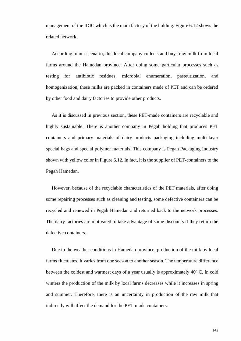
142

management of the IDIC which is the main factory of the holding. Figure 6.12 shows the

related network.

According to our scenario, this local company collects and buys raw milk from local

farms around the Hamedan province. After doing some particular processes such as

testing for antibiotic residues, microbial enumeration, pasteurization, and

homogenization, these milks are packed in containers made of PET and can be ordered

by other food and dairy factories to provide other products.

As it is discussed in previous section, these PET-made containers are recyclable and

highly sustainable. There is another company in Pegah holding that produces PET

containers and primary materials of dairy products packaging including multi-layer

special bags and special polymer materials. This company is Pegah Packaging Industry

shown with yellow color in Figure 6.12. In fact, it is the supplier of PET-containers to the

Pegah Hamedan.

However, because of the recyclable characteristics of the PET materials, after doing

some repairing processes such as cleaning and testing, some defective containers can be

recycled and renewed in Pegah Hamedan and returned back to the network processes.

The dairy factories are motivated to take advantage of some discounts if they return the

defective containers.

Due to the weather conditions in Hamedan province, production of the milk by local

farms fluctuates. It varies from one season to another season. The temperature difference

between the coldest and warmest days of a year usually is approximately 40˚󠄙 C. In cold

winters the production of the milk by local farms decreases while it increases in spring

and summer. Therefore, there is an uncertainty in production of the raw milk that

indirectly will affect the demand for the PET-made containers.

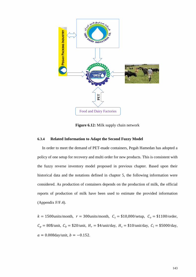
143

Figure 6.12: Milk supply chain network

6.3.4 Related Information to Adapt the Second Fuzzy Model

In order to meet the demand of PET-made containers, Pegah Hamedan has adopted a

policy of one setup for recovery and multi order for new products. This is consistent with

the fuzzy reverse inventory model proposed in previous chapter. Based upon their

historical data and the notations defined in chapter 5, the following information were

considered. As production of containers depends on the production of milk, the official

reports of production of milk have been used to estimate the provided information

(Appendix F/F.4).

𝑘 = 1500units/month, 𝑟 = 300units/month, 𝐶𝑠 = $10,000/setup, 𝐶𝑜 = $1100/order,

𝐶𝑝 = 80$/unit, 𝐶𝑏 = $20/unit, 𝐻𝑟 = $4/unit/day, 𝐻𝑠 = $10/unit/day, 𝐶𝑙 = $5000/day,

𝑎 = 0.008day/unit, 𝑏 = −0.152.

Food and Dairy Factories

PE

T

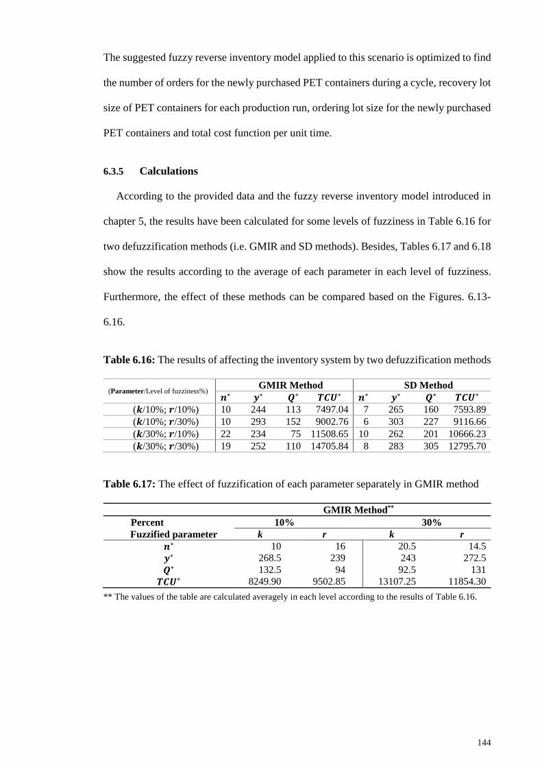
144

The suggested fuzzy reverse inventory model applied to this scenario is optimized to find

the number of orders for the newly purchased PET containers during a cycle, recovery lot

size of PET containers for each production run, ordering lot size for the newly purchased

PET containers and total cost function per unit time.

6.3.5 Calculations

According to the provided data and the fuzzy reverse inventory model introduced in

chapter 5, the results have been calculated for some levels of fuzziness in Table 6.16 for

two defuzzification methods (i.e. GMIR and SD methods). Besides, Tables 6.17 and 6.18

show the results according to the average of each parameter in each level of fuzziness.

Furthermore, the effect of these methods can be compared based on the Figures. 6.13-

6.16.

Table 6.16: The results of affecting the inventory system by two defuzzification methods

(Parameter/Level of fuzziness%) GMIR Method SD Method

𝒏∗ 𝒚∗ 𝑸∗ 𝑻𝑪𝑼∗ 𝒏∗ 𝒚∗ 𝑸∗ 𝑻𝑪𝑼∗ (𝒌/10%; 𝒓/10%) 10 244 113 7497.04 7 265 160 7593.89

(𝒌/10%; 𝒓/30%) 10 293 152 9002.76 6 303 227 9116.66

(𝒌/30%; 𝒓/10%) 22 234 75 11508.65 10 262 201 10666.23

(𝒌/30%; 𝒓/30%) 19 252 110 14705.84 8 283 305 12795.70

Table 6.17: The effect of fuzzification of each parameter separately in GMIR method

GMIR Method**

Percent 10% 30%

Fuzzified parameter k r k r

𝒏∗ 10 16 20.5 14.5

𝒚∗ 268.5 239 243 272.5

𝑸∗ 132.5 94 92.5 131

𝑻𝑪𝑼∗ 8249.90 9502.85 13107.25 11854.30

** The values of the table are calculated averagely in each level according to the results of Table 6.16.

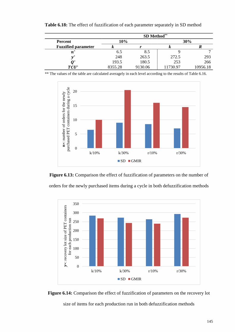
145

Table 6.18: The effect of fuzzification of each parameter separately in SD method

SD Method**

Percent 10% 30%

Fuzzified parameter k r k R

𝒏∗ 6.5 8.5 9 7

𝒚∗ 248 263.5 272.5 293

𝑸∗ 193.5 180.5 253 266

𝑻𝑪𝑼∗ 8355.28 9130.06 11730.97 10956.18

** The values of the table are calculated averagely in each level according to the results of Table 6.16.

Figure 6.13: Comparison the effect of fuzzification of parameters on the number of

orders for the newly purchased items during a cycle in both defuzzification methods

Figure 6.14: Comparison the effect of fuzzification of parameters on the recovery lot

size of items for each production run in both defuzzification methods

0

5

10

15

20

k/10% k/30% r/10% r/30%

𝒏∗:

num

ber

of

ord

ers

for

the

new

ly

purc

has

ed P

ET

co

nta

iner

s d

uri

ng a

cycl

e

SD GMIR

0

50

100

150

200

250

300

350

k/10% k/30% r/10% r/30%

𝒚∗:

rec

over

y l

ot

size

of

PE

T c

onta

iner

s

for

each

pro

duct

ion r

un

SD GMIR

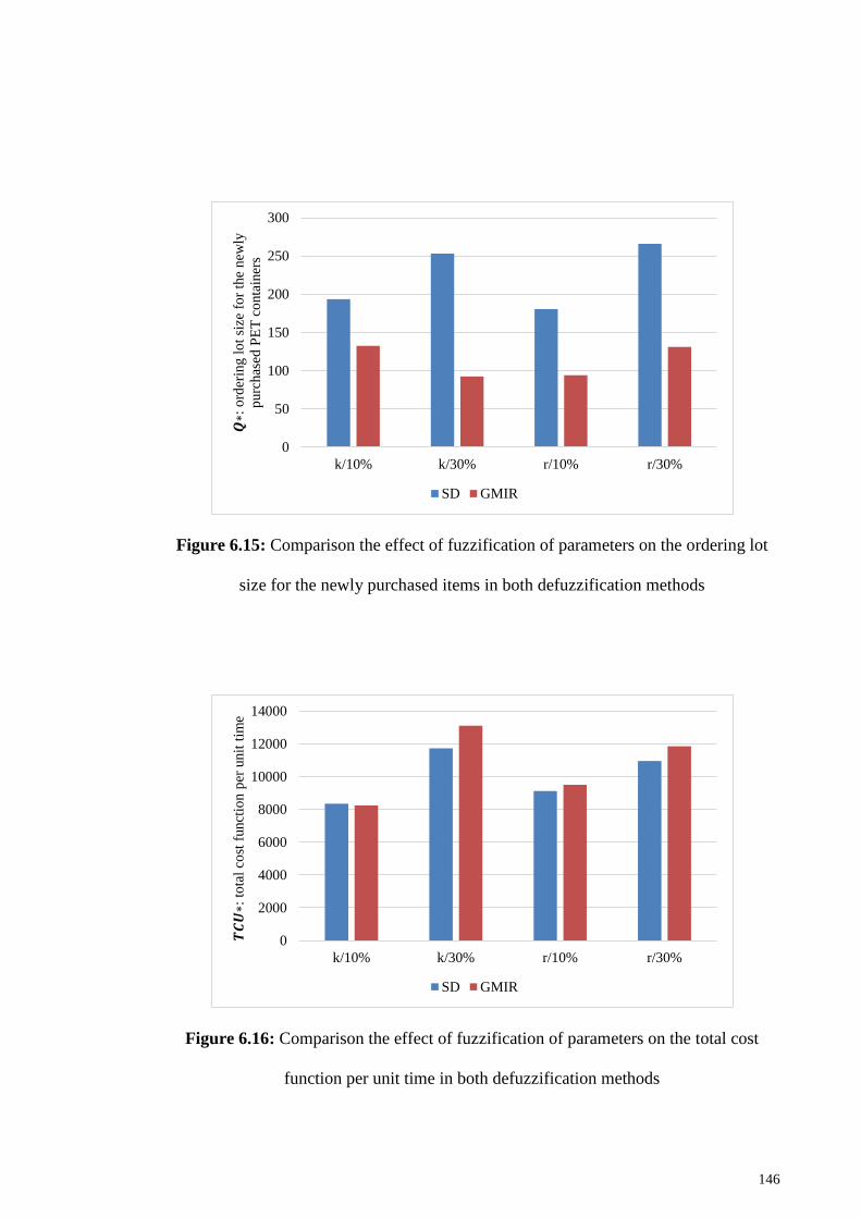
146

Figure 6.15: Comparison the effect of fuzzification of parameters on the ordering lot

size for the newly purchased items in both defuzzification methods

Figure 6.16: Comparison the effect of fuzzification of parameters on the total cost

function per unit time in both defuzzification methods

0

50

100

150

200

250

300

k/10% k/30% r/10% r/30%

𝑸∗:

ord

erin

g l

ot

size

fo

r th

e new

ly

purc

has

ed P

ET

co

nta

iner

s

SD GMIR

0

2000

4000

6000

8000

10000

12000

14000

k/10% k/30% r/10% r/30%

𝑻𝑪𝑼∗:

to

tal

cost

funct

ion p

er u

nit

tim

e

SD GMIR

147

6.3.6 Analyzing the Results

Table 6.16 shows the results for two different levels of fuzziness. As it is clear, in this

case when there is the lowest level of fuzziness in the system, the GMIR method gives

the lower total cost per unit time. On the other hand, for the maximum level of fuzziness,

the total cost per unit time derived by the SD method is lower.

Tables 6.17 and 6.18 show the results of each parameters separately for the GMIR and

SD methods respectively. These results are calculated based on the average of optimal

values of the system. As it is clear, in the GMIR method when the uncertainty of demand

increases, the optimal number of orders for the newly purchased PET containers

increases. However, this increase is less in SD method. The effect of uncertainty of return

rate on the optimal number of newly purchased items in both methods is lower as

compared to the demand. As can be seen in Table 6.18, increasing in the uncertainty of

demand or return rate leads to the increasing in the optimum value of recovery lot size

and ordering lot size for the newly purchased items. In GMIR method, by increasing in

the fuzziness of demand, the optimum value of recovery lot size and ordering lot size for

the newly purchased items, 10 and 30 percent decrease respectively. However, this

increase in the fuzziness of return rate cause to 12 and 39 percent increase in the optimum

value of recovery lot size and ordering lot size for the newly purchased items respectively.

Moreover, an interesting result is that regardless of the value of changes, as the

uncertainty increases, total cost per unit time in all level of both parameters increases.

Nonetheless the percent change of total costs that resulted from the SD method are less

than those that are obtained using the GMIR method.

In Figures 6.13-6.16, the effect of uncertainty has been mutually compared for both

defuzzification methods in each level of fuzziness for parameters on considered optimal

values.

148

Figure 6.13 shows that optimum number of orders for the newly purchased PET

containers in all levels of uncertainty of both parameters is higher for the GMIR method

as compared to the SD method. By analysing Figure 6.14, it can be deduced that the

optimal recovery lot size derived by the GMIR method in all level of fuzziness for the

fuzzified parameters is more than the ones derived by the SD method. Furthermore, as it

is clear from the Figure 6.15, higher ordering lot size can be obtained by the SD method

with respect to the level of uncertainty and the fuzzified parameter. If the focus is on

uncertainty of one parameter, generally the total cost per unit time obtained by the SD

method is lower.

6.4 Chapter Summary

In this chapter, the fuzzy inventory models introduced in previous chapters are applied

in real applications. The applicability of the first fuzzy inventory model suggested in

chapter 4 is shown in automobile industry. Moreover, the practical application of the

second fuzzy reverse inventory model was represented through a real case from the milk

industry.

In both cases, the effect of uncertainty of fuzzified parameters is analyzed on the

considered optimal values in some level of fuzziness through some figures and tables.

According to the results obtained, it can be concluded that based on the strategy of the

company which method is more appropriate. For example, if the strategy is decreasing

the total cost, using the SD methods is more logical in the second investigated case study.

149

CHAPTER 7: CONCLUSION

7.1 Concluding Remarks

Inventory management is an integral and important part of a supply chain management

in business activities. It plays a vital role in different parts and processes of a company

that are related to the finished items and raw materials. Therefore, sufficient attentions

should be given to choose a proper inventory control system. Otherwise, organizations

suffer from losing the investment in inventory management. Inventory systems can be

investigated from many points of view.

In present research, attempts were made to design and formulate inventory systems

that are appropriate to deal with the volatile business environment, and at the same time,

they take some advantages. To do so, fuzzy set theory is combined with the investigated

inventory systems to obtain more robust results. It is shown that these kinds of fuzzy

inventory systems are more precious and they work better in real world. Because

uncertainty is an inherent part of the information systems especially for data in inventory

systems.

Another important characteristic that is taken into account is the learning process. As

usually inventory operations are affected by the learning phenomena and can be improved

during the time, the influence of uncertainty is studied with the learning theory

simultaneously. The results revealed that optimized values could be improved by passing

the time due to the effect of learning.

Moreover, other characteristics such as different holding costs for perfect and defective

items and return rate for the recovered items are considered. Two inventory systems

applying the mentioned theories (i.e. fuzzy set theory and learning theory) were

developed and optimized with mathematical procedures.

150

In order to highlight the contributions of the developed fuzzy inventory systems

through the previous researches, a comprehensive literature review was conducted

gathering more than 130 papers published in peer reviewed prestigious international

journals. The fuzzy inventory models of these researches were analyzed in details

analysing their contents. These models are divided in two main categories (i.e. economic

order quantity (EOQ) and economic production quantity (EPQ)), and studied these

models from some aspects including membership functions and methods and techniques

for fuzzification, defuzzification and optimization. It was the first time that such a

complete review was done in the fuzzy inventory models literature.

In the first model, a fully fuzzy inventory system was presented with a total cost

function including variable and fixed costs, selling prices of good and defective quality

items, holding costs of defective and non-defective items, screening rate and screening

costs. Besides, it was supposed that percentage of defective items per shipment decreases

during the cycles and it follows a S-shaped logistic learning curve model. All parameters

and variables of the model are assumed as triangular fuzzy numbers to show an inventory

model that is appropriate in an uncertain environment.

The objective was to obtain the lot size in 𝑛th shipment when learning occurs

minimizing the total cost function. After obtaining the defuzzified total cost function

applying the GMIR method, the conditions of KKT theorem were analyzed, and then, the

problem was optimized by derivation. In order to test the investigated model, a numerical

example is provided and the effect of learning and fuzziness is analyzed simultaneously

on the total profit per unit time and order quantity.

It is concluded that the optimal lot size directly depends on the amount of uncertainty.

It was shown that it increases when the level of uncertainty of the inventory system

increases. To avoid costly inventory strategy, it is necessary to reduce the impreciseness

151

of the model. It is proved that the decision maker should expect an increase in the total

profit when learning occurs and it justifies some costs that are devoted to the learning

process in the long-term.

The inventory system that is completely fuzzified is compared with the partially

fuzzified one. It was shown that the real inventory situation that is affected by uncertainty

can be captured if more elements are fuzzified. However, sometimes it causes complex

and complicated models which are difficult to be optimized. Moreover, the effect of

learning is more tangible on the optimal EOQ for the fully fuzzified model when the level

of uncertainty increases.

The third part of this thesis is devoted to study the effect of fuzziness of demand and

collection rate of the recoverable products from customers through a reverse inventory

model which was partially fuzzified. The effect of two defuzzification methods (i.e.

GMIR and SD methods) is compared and analyzed. The defuzzified total cost function of

the model including setup cost for the recovery process, ordering cost for the newly

purchased products, inventory holding costs of collected and serviceable products, labour

production cost, unit purchase cost for the newly purchased products and unit buyback

cost for the recovered products was optimized by a one-dimensional search procedure.

Recovery lot size for each production run and number of orders for the newly purchased

products during a cycle were derived.

Proposing a comprehensive numerical example, the behaviour of the decision

variables were analyzed while the upper and lower bound of fuzzified parameters were

changed. As the results of these defuzzification methods are different in practice, optimal

fuzzy values in considered iterations are compared with similar crisp ones. It is shown

that when the levels of fuzziness were similar and the optimal number of orders were

equal, the percentage changes of the optimal recovery lot size in the GMIR method were

152

negative as compared to the SD method. Moreover, in the case that upper bound of return

rate was greater than the lower bound in triangular fuzzy numbers, the percentage changes

of the optimal total cost by the signed distance method were negative. When it was

smaller than the lower bound, those were positive in all cases.

In order to show the applicability of the proposed fuzzy inventory models, these

models are used in two real cases. The first case was related to investigation of an

inventory system in a supply chain for the automobile industry. Optimal order quantities

and total profit per unit time of Brake Disc and Rear Hub Drum are found for low and

high uncertain levels. It is concluded that the more the level of fuzziness, the more the

effect of learning.

Furthermore, the second fuzzy model which was a reverse EOQ inventory system was

explained in the milk industry. In the supply chain of a milk manufacturing company,

there was a material called PET for packaging in which could be recovered. The number

of orders for the newly purchased PET during a cycle, the recovery lot size of PET for

each production run, the ordering lot size for the newly purchased PET and the total cost

function per unit time for a local milk manufacturing company are found. Regarding the

total cost per unit time, it is shown that the behavior of the investigated defuzzification

methods are different.

7.2 Contributions and Applications

In this section, the contribution of this research is explained dividing it into two

sections that are related to the knowledge and application.

7.2.1 Contribution to the Knowledge

The first fuzzy inventory model that was developed showed a fully fuzzy system. An

inventory system that is completely fuzzified generally is very hard to be optimized.

153

However, the proposed fully fuzzy model was solved using a mathematical algorithm.

Although there are many studies in the previous literature, almost all of them considered

a partially uncertain system. It means that these models usually target a special parameter

or variable and study the effect of uncertainty on the considered element. However, there

are models with more than one element that is fuzzified but not to the explained problem.

Learning theory can be observed in the previous inventory literature. In present

research, the effect of fuzziness and learning is studied simultaneously where the

inventory system is affected by a fully fuzzified learning function. This provides the

opportunity to examine the behavior of optimal lot size and optimal total profit in such a

situation to make the best strategy.

In the second model, the rate of return was targeted in an uncertain environment where

the recovery production of the system is improved due to the learning by passing the time.

This was the first time that the effect of fuzzification of two defuzzification methods was

analyzed and compared in a partially fuzzified reverse inventory system. This provides

the opportunity to select the best decision according to the situation of the company.

7.2.2 Contribution to the Practitioners

As uncertainty is an inherent part of the real world, inventory models that combine

fuzzy set theory with the inventory system have many applications in the real world. As

almost nothing is constant in real business environment, the developed fully fuzzified

model can be very helpful to depict the best strategy. Moreover, learning theory can be

applied in each inventory system that the related process could be improved during the

cycles. Besides, other investigated characteristics such as imperfect quality items have

practical applications in the real inventory systems. The rate of return in a reverse

inventory system is a very important factor that can influence the whole of a supply chain.

154

In any industry that produced or supplied product can be recovered, it plays an important

role.

As it is discussed in previous chapter, the developed fuzzy forward and backward

models of this thesis can have many applications in real world considering their

characteristics. In addition to the discussed applications in chapter 6, first model can apply

in semiconductor industries because they usually separate defective and non-defective

items. Moreover, second model can have some applications in food and beverage

industries. Because they usually supply items in containers that should be recovered due

to the environment concerns. Moreover, both models can be used in any industry that

deals with defective items.

7.3 Recommendations for Future Research

There are several opportunities to extend this research in the future. Regardless of the

complexity of calculations, alternative defuzzification methods such as centroid method

could be applied and the results could be compared and analyzed. Besides, other types of

fuzzy numbers, such as trapezoidal fuzzy number, could be investigated on the behavior

of the fuzzified parameters.

Another room for future research that would be of interest is studying the fuzzy

inventory models if learning in fuzziness is occurred. This is for the situation that

uncertainty decreases over time because of the effect of learning process. These

conditions can on the upper and lower bounds of a triangular fuzzy number.

It may also be of interest to incorporate different types of learning functions to evaluate

and compare the results. Also the models can be develop combining the learning with

other parameters that have potentials to be improved during the time. In such a scenario,

learning curves with different learning ratio could be investigated.

155

Although this is the first attempt to apply fuzzy set theory in the reverse inventory

literature, future works can apply these methods on the other reverse EOQ/EPQ models

with other assumptions and conditions.

156

REFERENCES

Bag, S., Chakraborty, D., & Roy, A. (2009). A production inventory model with fuzzy

random demand and with flexibility and reliability considerations. Computers &

Industrial Engineering, 56(1), 411-416.

Bansal, A. (2011). Trapezoidal fuzzy numbers (a, b, c, d): Arithmetic behavior.

International Journal of Physical and Mathematical Sciences, 2(1), 39-44.

Baykasoglu, A., & Gocken, T. (2011). Solving fully fuzzy mathematical programming

model of EOQ problem with a direct approach based on fuzzy ranking and PSO.

Journal of Intelligent & Fuzzy Systems: Applications in Engineering and

Technology, 22(5), 237-251.

Baykasoğlu, A., & Göçken, T. (2007). Solution of a fully fuzzy multi-item economic

order quantity problem by using fuzzy ranking functions. Engineering

Optimization, 39(8), 919-939.

Bera, U., Maiti, M. K., & Maiti, M. (2012). Inventory model with fuzzy lead-time and

dynamic demand over finite time horizon using a multi-objective genetic

algorithm. Computers & Mathematics with Applications, 64(6), 1822-1838.

Björk, K.-M. (2009). An analytical solution to a fuzzy economic order quantity problem.

International Journal of Approximate Reasoning, 50(3), 485-493.

Björk, K.-M. (2012). A multi-item fuzzy economic production quantity problem with a

finite production rate. International Journal of Production Economics, 135(2),

702-707.

Buzacott, J. (1975). Economic order quantities with inflation. Operational research

quarterly, 26(3), 553-558.

Chakrabortty, S., Pal, M., & Nayak, P. K. (2013). Intuitionistic fuzzy optimization

technique for Pareto optimal solution of manufacturing inventory models with

shortages. European Journal of Operational Research, 228(2), 381-387.

Chakraborty, N., Mondal, S., & Maiti, M. (2013). A deteriorating multi-item inventory

model with price discount and variable demands via fuzzy logic under resource

constraints. Computers & Industrial Engineering, 66(4), 976-987.

Chang, C.-T., Ouyang, L.-Y., & Teng, J.-T. (2003). An EOQ model for deteriorating

items under supplier credits linked to ordering quantity. Applied Mathematical

Modelling, 27(12), 983-996.

Chang, H.-C. (2003). Fuzzy opportunity cost for EOQ model with quality improvement

investment. International Journal of Systems Science, 34(6), 395-402.

Chang, H.-C. (2004). An application of fuzzy sets theory to the EOQ model with

imperfect quality items. Computers & Operations Research, 31(12), 2079-2092.

157

Chang, P.-T., & Chang, C.-H. (2006). An elaborative unit cost structure-based fuzzy

economic production quantity model. Mathematical and Computer Modelling,

43(11), 1337-1356.

Chang, P.-T., Yao, M.-J., Huang, S.-F., & Chen, C.-T. (2006). A genetic algorithm for

solving a fuzzy economic lot-size scheduling problem. International Journal of

Production Economics, 102(2), 265-288.

Chang, S.-C. (1999). Fuzzy production inventory for fuzzy product quantity with

triangular fuzzy number. Fuzzy sets and Systems, 107(1), 37-57.

Chang, S.-C., Yao, J.-S., & Lee, H.-M. (1998). Economic reorder point for fuzzy

backorder quantity. European Journal of Operational Research, 109(1), 183-202.

Chen, L.-H., & Ouyang, L.-Y. (2006). Fuzzy inventory model for deteriorating items with

permissible delay in payment. Applied Mathematics and Computation, 182(1),

711-726.

Chen, S.-H. (1985). Operations on fuzzy numbers with function principle. Tamkang

Journal of Management Sciences, 6(1), 13-26.

Chen, S.-H., Wang, C.-C., & Arthur, R. (1996). Backorder fuzzy inventory model under

function principle. Information Sciences, 95(1), 71-79.

Chen, S. H., & Chang, S. M. (2008). Optimization of fuzzy production inventory model

with unrepairable defective products. International Journal of Production

Economics, 113(2), 887-894.

Chen, S. H., & Hsieh, C. H. (1999). Graded mean integration representation of

generalized fuzzy numbers. Journal of Chinese Fuzzy Systems, 5, 1-7.

Chen, Y.-C. (2003). A probabilistic approach for traditional EOQ model. Journal of

Information and Optimization Sciences, 24(2), 249-253.

Chou, S.-Y., Julian, P. C., & Hung, K.-C. (2009). A note on fuzzy inventory model with

storage space and budget constraints. Applied Mathematical Modelling, 33(11),

4069-4077.

Das, B., & Maiti, M. (2013). Fuzzy stochastic inequality and equality possibility

constraints and their application in a production-inventory model via optimal

control method. Journal of Computational Science, 4(5), 360-369.

Das, D., Roy, A., & Kar, S. (2011). A volume flexible economic production lot-sizing

problem with imperfect quality and random machine failure in fuzzy-stochastic

environment. Computers & Mathematics with Applications, 61(9), 2388-2400.

Das, K., Roy, T., & Maiti, M. (2000). Multi-item inventory model with quantity-

dependent inventory costs and demand-dependent unit cost under imprecise

objective and restrictions: a geometric programming approach. Production

Planning & Control, 11(8), 781-788.

158

Das, K., Roy, T. K., & Maiti, M. (2004). Multi-item stochastic and fuzzy-stochastic

inventory models under two restrictions. Computers & Operations Research,

31(11), 1793-1806.

De, S. K., & Goswami, A. (2006). An EOQ model with fuzzy inflation rate and fuzzy

deterioration rate when a delay in payment is permissible. International Journal

of Systems Science, 37(5), 323-335.

De, S. K., Goswami, A., & Sana, S. S. (2014). An interpolating by pass to Pareto

optimality in intuitionistic fuzzy technique for a EOQ model with time sensitive

backlogging. Applied Mathematics and Computation, 230, 664-674.

De, S. K., & Sana, S. S. (2013a). Backlogging EOQ model for promotional effort and

selling price sensitive demand- an intuitionistic fuzzy approach. Annals of

Operations Research, 233(1), 57-76.

De, S. K., & Sana, S. S. (2013b). Fuzzy order quantity inventory model with fuzzy

shortage quantity and fuzzy promotional index. Economic Modelling, 31, 351-

358.

De, S. K., & Sana, S. S. (2014). A multi-periods production–inventory model with

capacity constraints for multi-manufacturers–A global optimality in intuitionistic

fuzzy environment. Applied Mathematics and computation, 242, 825-841.

Farhoodi, M., Emam-Djomeh, Z., Falah, A., Sabetghadam, S., & Nemati, M. (2013).

Effect of menthol absorption by packaging material on the quality of yogurt drink

during storage time. Journal of Agricultural Science and Technology, 15, 1373-

1380.

Farhoodi, M., Emam-Djomeh, Z., Oromiehie, A., & Ehsani, M. R. (2009). Influence of

menthol absorption on the mechanical properties of PET bottles. Iranian Polymer

Journal, 18(3), 227-232.

Flapper, S. D. P. (1996). One-way or reusable distribution items. Paper presented at the

Proceedings of the second international conference on computer integrated

manufacturing in the process industries. , The Netherlands: EindhovenUniversity

of Technology

Glock, C. H. (2012). The joint economic lot size problem: A review. International

Journal of Production Economics, 135(2), 671-686.

Govindan, G., Soleimani, H., & Kannanc, D. (2015). Reverse logistics and closed-loop

supply chain: A comprehensive review to explore the future. European Journal

of Operational Research, 240(3), 603-626.

Guchhait, P., Maiti, M. K., & Maiti, M. (2015). An EOQ model of deteriorating item in

imprecise environment with dynamic deterioration and credit linked demand.

Applied Mathematical Modelling, 39(21), 6553-6567.

Guchhait, P., Maiti, M. K., & Maiti, M. (2010). Multi-item inventory model of breakable

items with stock-dependent demand under stock and time dependent breakability

rate. Computers & Industrial Engineering, 59(4), 911-920.

159

Guchhait, P., Maiti, M. K., & Maiti, M. (2013). A production inventory model with fuzzy

production and demand using fuzzy differential equation: an interval compared

genetic algorithm approach. Engineering Applications of Artificial Intelligence,

26(2), 766-778.

Guchhait, P., Maiti, M. K., & Maiti, M. (2014). Inventory policy of a deteriorating item

with variable demand under trade credit period. Computers & Industrial

Engineering, 76, 75-88.

Guiffrida, A. (2009). Fuzzy inventory models (M. Y. Jaber Ed.): Boca Raton: CRC Press.

Halim, K., Giri, B. C., & Chaudhuri, K. (2009). Fuzzy EPQ models for an imperfect

production system. International Journal of Systems Science, 40(1), 45-52.

Harris, F. W. (1913). How many parts to make at once. Factory: The Magazine of

Management, 10(2), 135-136, 152.

Hillier, F., & Lieberman, G. (2001). Introduction to Operations Research, McGraw Hill.

New York.

Hochrein, S., & Glock, C. H. (2012). Systematic literature reviews in purchasing and

supply management research: a tertiary study. International Journal of Integrated

Supply Management, 7(4), 215-245.

Hojati, M. (2004). Bridging the gap between probabilistic and fuzzy-parameter EOQ

models. International Journal of Production Economics, 91(3), 215-221.

Hsieh, C. H. (2002). Optimization of fuzzy production inventory models. Information

Sciences, 146(1), 29-40.

Hsu, W. (2012). Optimal inventory model with fuzzy perfective rate, demand rate, and

purchasing cost under immediate return for defective items. International Journal

of Innovative Computing, Information and Control, 8, 2583-2598.

Hu, J.-S., Zheng, H., Guo, C.-Y., & Ji, Y.-P. (2010). Optimal production run length with

imperfect production processes and backorder in fuzzy random environment.

Computers & Industrial Engineering, 59(1), 9-15.

Huang, T.-T. (2011). Fuzzy multilevel lot-sizing problem based on signed distance and

centroid. International Journal of Fuzzy Systems, 13(2), 98-110.

Islam, S., & Roy, T. K. (2006). A fuzzy EPQ model with flexibility and reliability

consideration and demand dependent unit production cost under a space

constraint: A fuzzy geometric programming approach. Applied Mathematics and

Computation, 176(2), 531-544.

Islam, S., & Roy, T. K. (2007). Fuzzy multi-item economic production quantity model

under space constraint: A geometric programming approach. Applied

Mathematics and Computation, 184(2), 326-335.

160

Jaber, M., Goyal, S., & Imran, M. (2008). Economic production quantity model for items

with imperfect quality subject to learning effects. International Journal of


Jaber, M. Y., & El Saadany, A. M. (2011). An economic production and remanufacturing

model with learning effects. International Journal of Production Economics,

131(1), 115-127.

Jamal, A., Sarker, B., & Wang, S. (1997). An ordering policy for deteriorating items with

allowable shortage and permissible delay in payment. Journal of the Operational

Research Society, 48(8), 826-833.

Jana, D. K., Das, B., & Maiti, M. (2014). Multi-item partial backlogging inventory models

over random planninghorizon in random fuzzy environment. Applied Soft

Computing, 21, 12-27.

Jana, D. K., Maity, K., Das, B., & Roy, T. K. (2013). A fuzzy simulation via contractive

mapping genetic algorithm approach to an imprecise production inventory model

under volume flexibility. Journal of Simulation, 7(2), 90-100.

Kacprzyk, J., & Stanieski, P. (1982). Long-term inventory policy-making through fuzzy

decision-making models. Fuzzy sets and Systems, 8(2), 117-132.

Kaufman, A., & Gupta, M. M. (1991). Introduction to fuzzy arithmetic: theory and

application. New York: VanNostrand Reinhold.

Kazemi, N., Ehsani, E., & Jaber, M. (2010). An inventory model with backorders with

fuzzy parameters and decision variables. International Journal of Approximate

Reasoning, 51(8), 964-972.

Kazemi, N., Shekarian, E., Cárdenas-Barrón, L. E., & Olugu, E. U. (2015). Incorporating

human learning into a fuzzy EOQ inventory model with backorders. Computers

& Industrial Engineering, 87, 540-542.

Ketsarapong, S., Punyangarm, V., Phusavat, K., & Lin, B. (2012). An experience-based

system supporting inventory planning: A fuzzy approach. Expert Systems with

Applications, 39(8), 6994-7003.

Khan, M., Jaber, M., Guiffrida, A., & Zolfaghari, S. (2011b). A review of the extensions

of a modified EOQ model for imperfect quality items. International Journal of


Khan, M., Jaber, M. Y., & Bonney, M. (2011a). An economic order quantity (EOQ) for

items with imperfect quality and inspection errors. International Journal of


Kumar, R. S., & Goswami, A. (2015a). A continuous review production–inventory

system in fuzzy random environment: Minmax distribution free procedure.

Computers & Industrial Engineering, 79, 65-75.

161

Kumar, R. S., & Goswami, A. (2015b). EPQ model with learning consideration, imperfect

production and partial backlogging in fuzzy random environment. International

Journal of Systems Science, 46(8), 1486-1497.

Kumar, R. S., & Goswami, A. (2015c). A fuzzy random EPQ model for imperfect quality

items with possibility and necessity constraints. Applied Soft Computing, 34, 838-

850.

Lee, H.-M., & Lin, L. (2011). Applying signed distance method for fuzzy inventory

without backorder. International Journal of Innovative Computing, Information

and Control, 7(6), 3523-3531.

Lee, H.-M., & Yao, J.-S. (1998). Economic production quantity for fuzzy demand

quantity, and fuzzy production quantity. European Journal of Operational

Research, 109(1), 203-211.

Lee, H.-M., & Yao, J.-S. (1999). Economic order quantity in fuzzy sense for inventory

without backorder model. Fuzzy sets and Systems, 105(1), 13-31.

Lin, D.-C., & Yao, J.-S. (2000). Fuzzy economic production for production inventory.

Fuzzy Sets and Systems, 111(3), 465-495.

Lin, Y.-J. (2008). Minimax distribution free procedure with backorder price discount.

International Journal of Production Economics, 111(1), 118-128.

Liu, S.-T. (2008). Fuzzy profit measures for a fuzzy economic order quantity model.


Maddah, B., & Jaber, M. Y. (2008). Economic order quantity for items with imperfect

quality: revisited. International Journal of Production Economics, 112(2), 808-

815.

Mahapatra, G., Mandal, T., & Samanta, G. (2011). A production inventory model with

fuzzy coefficients using parametric geometric programming approach.

International Journal of Machine Learning and Cybernetics, 2(2), 99-105.

Mahapatra, N., & Maiti, M. (2006). Production–inventory model for a deteriorating item

with imprecise preparation time for production in a finite time horizon. Asia-

Pacific Journal of Operational Research, 23(2), 171-192.

Mahata, G., & Goswami, A. (2007). An EOQ model for deteriorating items under trade

credit financing in the fuzzy sense. Production Planning and Control, 18(8), 681-

692.

Mahata, G. C. (2015). A production-inventory model with imperfect production process

and partial backlogging under learning considerations in fuzzy random

environments. Journal of Intelligent Manufacturing, 1-15.

Mahata, G. C., & Goswami, A. (2013). Fuzzy inventory models for items with imperfect

quality and shortage backordering under crisp and fuzzy decision variables.


162

Mahata, G. C., & Mahata, P. (2011). Analysis of a fuzzy economic order quantity model

for deteriorating items under retailer partial trade credit financing in a supply

chain. Mathematical and Computer Modelling, 53(9), 1621-1636.

Maiti, M. K. (2008). Fuzzy inventory model with two warehouses under possibility

measure on fuzzy goal. European Journal of Operational Research, 188(3), 746-

774.

Maiti, M. K. (2011). A fuzzy genetic algorithm with varying population size to solve an

inventory model with credit-linked promotional demand in an imprecise planning

horizon. European Journal of Operational Research, 213(1), 96-106.

Maiti, M. K., & Maiti, M. (2007). Two storage inventory model in a mixed environment.

Fuzzy Optimization and Decision Making, 6(4), 391-426.

Maity, A., Maity, K., & Maiti, M. (2008). A production–recycling–inventory system with

imprecise holding costs. Applied Mathematical Modelling, 32(11), 2241-2253.

Maity, A. K. (2011a). One machine multiple-product problem with production-inventory

system under fuzzy inequality constraint. Applied Soft Computing, 11(2), 1549-

1555.

Maity, K. (2011b). Possibility and necessity representations of fuzzy inequality and its

application to two warehouse production-inventory problem. Applied

Mathematical Modelling, 35(3), 1252-1263.

Maity, K., & Maiti, M. (2005). Numerical approach of multi-objective optimal control

problem in imprecise environment. Fuzzy Optimization and Decision Making,

4(4), 313-330.

Maity, K., & Maiti, M. (2007). Possibility and necessity constraints and their

defuzzification—a multi-item production-inventory scenario via optimal control

theory. European Journal of Operational Research, 177(2), 882-896.

Maity, K., & Maiti, M. (2008). A numerical approach to a multi-objective optimal

inventory control problem for deteriorating multi-items under fuzzy inflation and

discounting. Computers & Mathematics with Applications, 55(8), 1794-1807.

Mandal, N. K., & Roy, T. K. (2006a). A displayed inventory model with L–R fuzzy

number. Fuzzy Optimization and Decision Making, 5(3), 227-243.

Mandal, N. K., & Roy, T. K. (2006b). Multi-item imperfect production lot size model

with hybrid number cost parameters. Applied Mathematics and computation,

182(2), 1219-1230.

Mandal, N. K., Roy, T. K., & Maiti, M. (2005). Multi-objective fuzzy inventory model

with three constraints: a geometric programming approach. Fuzzy Sets and

Systems, 150(1), 87-106.

Mandal, S., Maity, A., Maity, K., Mondal, S., & Maiti, M. (2011). Multi-item multi-

period optimal production problem with variable preparation time in fuzzy

stochastic environment. Applied Mathematical Modelling, 35(9), 4341-4353.

163

Mandal, S., Maity, K., Mondal, S., & Maiti, M. (2010). Optimal production inventory

policy for defective items with fuzzy time period. Applied Mathematical

Modelling, 34(3), 810-822.

Mayring, P. (2010). Qualitative Inhaltsanalyse. In G. Mey & K. Mruck (Eds.), Handbuch

Qualitative Forschung in der Psychologie (pp. 601-613): VS Verlag für

Sozialwissenschaften.

Mezei, J., & Björk, K.-M. (2015). An economic production quantity problem with

backorders and fuzzy cycle times. Journal of Intelligent & Fuzzy Systems:

Applications in Engineering and Technology, 28(4), 1861-1868.

Milenkovic, M., & Bojovic, N. (2014). Fuzzy modeling approach to the rail freight car

inventory problem. Transportation Planning and Technology, 37(2), 119-137.

Mondal, M., Maiti, M. K., & Maiti, M. (2014). A two storage production-repairing model

with fuzzy defective rate and displayed inventory dependent demand.

Optimization and Engineering, 15(3), 751-772.

Mondal, M., Maity, A. K., Maiti, M. K., & Maiti, M. (2013). A production-repairing

inventory model with fuzzy rough coefficients under inflation and time value of

money. Applied Mathematical Modelling, 37(5), 3200-3215.

Mondal, S., & Maiti, M. (2002). Multi-item fuzzy EOQ models using genetic algorithm.


Mousavi, S. M., Sadeghi, J., Niaki, S. T. A., Alikar, N., Bahreininejad, A., & Metselaar,

H. S. C. (2014). Two parameter-tuned meta-heuristics for a discounted inventory

control problem in a fuzzy environment. Information Sciences, 276, 42-62.

Nice, K. (2016). How drum brakes work. http://auto.howstuffworks.com/auto-

parts/brakes/brake-types/drum-brake.htm

Ouyang, L.-Y., Teng, J.-T., & Cheng, M.-C. (2010). A fuzzy inventory system with

deteriorating items under supplier credits linked to ordering quantity. Journal of

Information Science and Engineering, 26(1), 231-253.

Paknejad, J., Nasri, F., & Affisco, J. F. (2005). Quality improvement in an inventory

model with finite-range stochastic lead times. Advances in Decision Sciences,

2005(3), 177-189.

Pal, S., Mahapatra, G., & Samanta, G. (2014). An EPQ model of ramp type demand with

Weibull deterioration under inflation and finite horizon in crisp and fuzzy

environment. International Journal of Production Economics, 156, 159-166.

Pal, S., Mahapatra, G., & Samanta, G. (2015). A production inventory model for

deteriorating item with ramp type demand allowing inflation and shortages under

fuzziness. Economic Modelling, 46, 334-345.

Pal, S., Maiti, M. K., & Maiti, M. (2009). An EPQ model with price discounted

promotional demand in an imprecise planning horizon via genetic algorithm.


164

Panda, D., Kar, S., & Maiti, M. (2008a). Multi-item EOQ model with hybrid cost

parameters under fuzzy/fuzzy-stochastic resource constraints: a geometric

programming approach. Computers & Mathematics with Applications, 56(11),

2970-2985.

Panda, D., Kar, S., Maity, K., & Maiti, M. (2008b). A single period inventory model with

imperfect production and stochastic demand under chance and imprecise

constraints. European Journal of Operational Research, 188(1), 121-139.

Panda, D., & Maiti, M. (2009). Multi-item inventory models with price dependent

demand under flexibility and reliability consideration and imprecise space

constraint: A geometric programming approach. Mathematical and Computer

Modelling, 49(9), 1733-1749.

Panda, D., Rong, M., & Maiti, M. (2014). Fuzzy mixture two warehouse inventory model

involving fuzzy random variable lead time demand and fuzzy total demand.

Central European Journal of Operations Research, 22(1), 187-209.

Pappis, C., & Karacapilidis, N. (1995). Lot size scheduling using fuzzy numbers.

International Transactions in Operational Research, 2(2), 205-212.

Park, K. S. (1987). Fuzzy-set theoretic interpretation of economic order quantity. Systems,

Man and Cybernetics, IEEE Transactions on, 17(6), 1082-1084.

Paul, S. K., Azeem, A., Sarker, R., & Essam, D. (2014). Development of a production

inventory model with uncertainty and reliability considerations. Optimization and

Engineering, 15(3), 697-720.

Porteus, E. L. (1986). Optimal lot sizing, process quality improvement and setup cost

reduction. Operations Research, 34(1), 137-144.

Rong, M., Mahapatra, N., & Maiti, M. (2008). A two warehouse inventory model for a

deteriorating item with partially/fully backlogged shortage and fuzzy lead time.

European Journal of Operational Research, 189(1), 59-75.

Roy, A., Kar, S., & Maiti, M. (2008). A deteriorating multi-item inventory model with

fuzzy costs and resources based on two different defuzzification techniques.


Roy, A., Maiti, M. K., Kar, S., & Maiti, M. (2007). Two storage inventory model with

fuzzy deterioration over a random planning horizon. Mathematical and Computer

Modelling, 46(11–12), 1419-1433.

Roy, A., Maiti, M. K., Kar, S., & Maiti, M. (2009a). An inventory model for a

deteriorating item with displayed stock dependent demand under fuzzy inflation

and time discounting over a random planning horizon. Applied Mathematical

Modelling, 33(2), 744-759.

Roy, A., Maity, K., & Maiti, M. (2009b). A production–inventory model with

remanufacturing for defective and usable items in fuzzy-environment. Computers

& Industrial Engineering, 56(1), 87-96.

165

Roy, T., & Maiti, M. (1997). A fuzzy EOQ model with demand-dependent unit cost under

limited storage capacity. European Journal of Operational Research, 99(2), 425-

432.

Roy, T., & Maiti, M. (1998). Multi-objective inventory models of deteriorating items with

some constraints in a fuzzy environment. Computers & Operations Research,

25(12), 1085-1095.

Roy, T. K., & Maiti, M. (1995). A fuzzy inventory model with a constraint. OPSEARCH,

32(4), 287-297.

Sadjadi, S. J., Ghazanfari, M., & Yousefli, A. (2010). Fuzzy pricing and marketing

planning model: A possibilistic geometric programming approach. Expert

Systems with Applications, 37(4), 3392-3397.

Saha, A., Roy, A., Kar, S., & Maiti, M. (2010). Inventory models for breakable items with

stock dependent demand and imprecise constraints. Mathematical and Computer

Modelling, 52(9), 1771-1782.

Salameh, M., & Jaber, M. (2000). Economic production quantity model for items with

imperfect quality. International Journal of Production Economics, 64(1), 59-64.

Samadi, F., Mirzazadeh, A., & Pedram, M. M. (2013). Fuzzy pricing, marketing and

service planning in a fuzzy inventory model: A geometric programming approach.


Samal, N., & Pratihar, D. (2014). Optimization of variable demand fuzzy economic order

quantity inventory models without and with backordering. Computers &

Industrial Engineering, 78, 148-162.

Shekarian, E., Glock, C. H., Amiri, S. M. P., & Schwindl, K. (2014a). Optimal

manufacturing lot size for a single-stage production system with rework in a fuzzy

environment. Journal of Intelligent & Fuzzy Systems: Applications in Engineering

and Technology, 27, 3067-3080.

Shekarian, E., Jaber, M. Y., Kazemi, N., & Ehsani, E. (2014b). A fuzzified version of the

economic production quantity (EPQ) model with backorders and rework for a

single-stage system. European Journal of Industrial Engineering, 8(3), 291-324.

Sommer, G. (1981). Fuzzy inventory scheduling. in Lasker, G. (Ed.) Applied systems and

cybernetics, VI, 3052-3060. Pergamon Press, New York.

Soni, H., & Shah, N. H. (2011). Optimal policy for fuzzy expected value production

inventory model with imprecise production preparation-time. International

Journal of Machine Learning and Cybernetics, 2(4), 219-224.

Soni, H. N., & Joshi, M. (2013). A fuzzy framework for coordinating pricing and

inventory policies for deteriorating items under retailer partial trade credit

financing. Computers & Industrial Engineering, 66(4), 865-878.

166

Sox, C. R., Jackson, P. L., Bowman, A., & Muckstadt, J. A. (1999). A review of the

stochastic lot scheduling problem. International Journal of Production

Economics, 62(3), 181-200.

Syed, J., & Aziz, L. (2007). Fuzzy inventory model without shortages using signed

distance method. Applied Mathematics & Information Sciences, 1(2), 203-209.

Taft, E. (1918). The most economical production lot. Iron Age, 101(18), 1410-1412.

Taha, H. A. (1997). Operations Research: An Introduction. New Jersey, USA: Prentice-

Hall.

Taleizadeh, A. A., Niaki, S. T. A., & Nikousokhan, R. (2011). Constraint multiproduct

joint-replenishment inventory control problem using uncertain programming.

Applied Soft Computing, 11(8), 5143-5154.

Taleizadeh, A. A., Wee, H.-M., & Jolai, F. (2013). Revisiting a fuzzy rough economic

order quantity model for deteriorating items considering quantity discount and

prepayment. Mathematical and Computer Modelling, 57(5), 1466-1479.

Tsai, D.-M. (2012). Optimal ordering and production policy for a recoverable item

inventory system with learning effect. International Journal of Systems Science,

43(2), 349-367.

Vijayan, T., & Kumaran, M. (2009). Fuzzy economic order time models with random

demand. International Journal of Approximate Reasoning, 50(3), 529-540.

Vujošević, M., Petrović, D., & Petrović, R. (1996). EOQ formula when inventory cost is

fuzzy. International Journal of Production Economics, 45(1), 499-504.

Wahab, M., & Jaber, M. (2010). Economic order quantity model for items with imperfect

quality, different holding costs, and learning effects: A note. Computers &

Industrial Engineering, 58(1), 186-190.

Wang, L., Fu, Q.-L., Lee, C.-G., & Zeng, Y.-R. (2013). Model and algorithm of fuzzy

joint replenishment problem under credibility measure on fuzzy goal. Knowledge-

Based Systems, 39, 57-66.

Wang, X., & Tang, W. (2009a). Fuzzy EPQ inventory models with backorder. Journal of

Systems Science and Complexity, 22(2), 313-323.

Wang, X., & Tang, W. (2009b). Optimal production run length in deteriorating

production processes with fuzzy elapsed time. Computers & Industrial

Engineering, 56(4), 1627-1632.

Wang, X., Tang, W., & Zhao, R. (2007a). Fuzzy economic order quantity inventory

models without backordering. Tsinghua Science & Technology, 12(1), 91-96.

Wang, X., Tang, W., & Zhao, R. (2007b). Random fuzzy EOQ model with imperfect

quality items. Fuzzy Optimization and Decision Making, 6(2), 139-153.

167

Wee, H.-M., Lo, C.-C., & Hsu, P.-H. (2009). A multi-objective joint replenishment

inventory model of deteriorated items in a fuzzy environment. European Journal


Wee, H. M., Yu, J., & Chen, M. C. (2007). Optimal inventory model for items with

imperfect quality and shortage backordering. Omega, 35(1), 7-11.

Whitin, T. M. (1954). Inventory control research: A survey. Management Science, 1(1),

32-40.

Wilson, R. (1934). A scientific routine for stock control. Harvard business review, 13(1),

116-129.

Winands, E. M., Adan, I. J., & Van Houtum, G. (2011). The stochastic economic lot

scheduling problem: A survey. European Journal of Operational Research,

210(1), 1-9.

Woodford, C. (2016). Brakes. In Explain that Stuff. Retrieved from

http://www.explainthatstuff.com/brakes.html

Wright, T. P. (1936). Factors affecting the cost of airplanes. Journal of the Aeronautical

Sciences, 3(4), 122-128. .

Wu, K., & Yao, J.-S. (2003). Fuzzy inventory with backorder for fuzzy order quantity

and fuzzy shortage quantity. European Journal of Operational Research, 150(2),

320-352.

Xu, J., & Liu, Y. (2008). Multi-objective decision making model under fuzzy random

environment and its application to inventory problems. Information Sciences,

178(14), 2899-2914.

Xu, J., & Zhao, L. (2008). A class of fuzzy rough expected value multi-objective decision

making model and its application to inventory problems. Computers &

Mathematics with Applications, 56(8), 2107-2119.

Xu, J., & Zhao, L. (2010). A multi-objective decision-making model with fuzzy rough

coefficients and its application to the inventory problem. Information Sciences,

180(5), 679-696.

Yadav, D., Singh, S., & Kumari, R. (2012a). Effect of demand boosting policy on optimal

inventory policy for imperfect lot saze with backorder in fuzzy environment.

Control and Cybernetics, 41, 191-212.

Yadav, D., Singh, S. R., Kumari, R., & Kumar, D. (2012b). Effects of learning on optimal

lot size and profit in fuzzy environment. International Journal of Operations and

Quantitative Management, 18, 145-158.

Yadav, D., Singh, S., & Kumari, R. (2013a). Application of minimax distribution free

procedure and chebyshev approach in mixed inventory model involving reducible

lead-time and setup cost with imprecise demand. Asia-Pacific Journal of

Operational Research, 30(4), 1350009.

168

Yadav, D., Singh, S., & Kumari, R. (2013b). Inventory model with learning effect and

imprecise market demand under screening error. OPSEARCH, 50(3), 418-432.

Yadav, D., Singh, S., & Kumari, R. (2015). Retailer's optimal policy under inflation in

fuzzy environment with trade credit. International Journal of Systems Science,

46(4), 754-762.

Yadavalli, V., Jeeva, M., & Rajagopalan, R. (2005). Multi-item deterministic fuzzy

inventory model. Asia-Pacific Journal of Operational Research, 22(3), 287-295.

Yaghin, R. G., Ghomi, S. F., & Torabi, S. A. (2013). A possibilistic multiple objective

pricing and lot-sizing model with multiple demand classes. Fuzzy Sets and

Systems, 231, 26-44.

Yao, J.-S., Chang, S.-C., & Su, J.-S. (2000). Fuzzy inventory without backorder for fuzzy

order quantity and fuzzy total demand quantity. Computers & Operations

Research, 27(10), 935-962.

Yao, J.-S., & Chiang, J. (2003). Inventory without backorder with fuzzy total cost and

fuzzy storing cost defuzzified by centroid and signed distance. European Journal


Yao, J.-S., & Lee, H.-M. (1996). Fuzzy inventory with backorder for fuzzy order quantity.

Information Sciences, 93(3), 283-319.

Yao, J.-S., & Lee, H.-M. (1999). Fuzzy inventory with or without backorder for fuzzy

order quantity with trapezoid fuzzy number. Fuzzy sets and Systems, 105(3), 311-

337.

Yao, J.-S., Ouyang, L.-Y., & Chang, H.-C. (2003). Models for a fuzzy inventory of two

replaceable merchandises without backorder based on the signed distance of fuzzy

sets. European Journal of Operational Research, 150(3), 601-616.

Yao, J.-S., & Su, J.-S. (2000). Fuzzy inventory with backorder for fuzzy total demand

based on interval-valued fuzzy set. European Journal of Operational Research,

124(2), 390-408.

Zadeh, L. A. (1965). Fuzzy sets. Information and control, 8(3), 338-353.

Zhang, C., Zhao, R., & Tang, W. (2009). Optimal run lengths in deteriorating production

processes in random fuzzy environments. Computers & Industrial Engineering,

57(3), 941-948.

Zimmermann, H.-J. (1975). Description and optimization of fuzzy systems. International

Journal of General System, 2(1), 209-215.

Zimmermann, H.-J. (2001). Fuzzy set theory—and its applications: Springer Science &

Business Media.

169

LIST OF PUBLICATIONS AND PAPERS PRESENTED

(a) Published

1. Shekarian, E., Olugu, E. U., Abdul-Rashid, S. H., & Kazemi, N. (2016). An economic

order quantity model considering different holding costs for imperfect quality items

subject to fuzziness and learning. Journal of Intelligent & Fuzzy Systems, 30(5),

2985–2997. (ISI, IOS Press)

2. Shekarian, E., Olugu, E. U., Abdul-Rashid, S. H., & Bottani, E. (2016). A fuzzy

reverse logistics inventory system integrating economic order/production quantity

models. International Journal of Fuzzy Systems, 18(6), 1141–1161. (ISI, Springer)

(b) Article in press

1. Shekarian, E., Kazemi, N., Olugu, E. U., & Abdul-Rashid, S. H. (2017). Fuzzy

inventory models: A comprehensive review. Applied Soft Computing. (ISI, Elsevier)

(c) Conference

1. Shekarian, E., Olugu, E. U., Abdul-Rashid, S. H., & Kazemi, N. (2016). Analyzing

optimization techniques in inventory models: the case of fuzzy economic order quantity

problems. Proceedings of the 2016 International Conference on Industrial Engineering

and Operations Management, Kuala Lumpur, Malaysia, March 8-10. (Awarded as the

Best Track Paper)

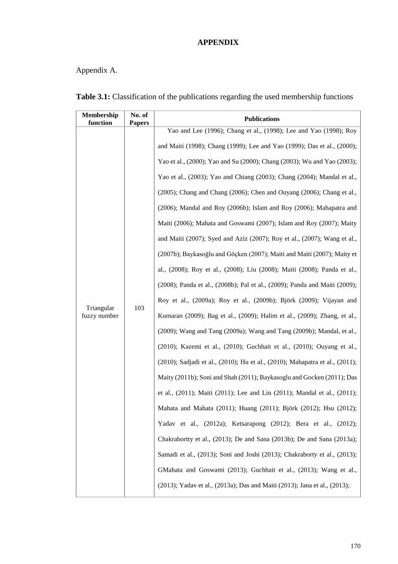
170

APPENDIX

Appendix A.

Table 3.1: Classification of the publications regarding the used membership functions

Membership

function

No. of

Papers Publications

Triangular

fuzzy number

103

Yao and Lee (1996); Chang et al., (1998); Lee and Yao (1998); Roy

and Maiti (1998); Chang (1999); Lee and Yao (1999); Das et al., (2000);

Yao et al., (2000); Yao and Su (2000); Chang (2003); Wu and Yao (2003);

Yao et al., (2003); Yao and Chiang (2003); Chang (2004); Mandal et al.,

(2005); Chang and Chang (2006); Chen and Ouyang (2006); Chang et al.,

(2006); Mandal and Roy (2006b); Islam and Roy (2006); Mahapatra and

Maiti (2006); Mahata and Goswami (2007); Islam and Roy (2007); Maity

and Maiti (2007); Syed and Aziz (2007); Roy et al., (2007); Wang et al.,

(2007b); Baykasoğlu and Göçken (2007); Maiti and Maiti (2007); Maity et

al., (2008); Roy et al., (2008); Liu (2008); Maiti (2008); Panda et al.,

(2008); Panda et al., (2008b); Pal et al., (2009); Panda and Maiti (2009);

Roy et al., (2009a); Roy et al., (2009b); Björk (2009); Vijayan and

Kumaran (2009); Bag et al., (2009); Halim et al., (2009); Zhang, et al.,

(2009); Wang and Tang (2009a); Wang and Tang (2009b); Mandal, et al.,

(2010); Kazemi et al., (2010); Guchhait et al., (2010); Ouyang et al.,

(2010); Sadjadi et al., (2010); Hu et al., (2010); Mahapatra et al., (2011);

Maity (2011b); Soni and Shah (2011); Baykasoglu and Gocken (2011); Das

et al., (2011); Maiti (2011); Lee and Lin (2011); Mandal et al., (2011);

Mahata and Mahata (2011); Huang (2011); Björk (2012); Hsu (2012);

Yadav et al., (2012a); Ketsarapong (2012); Bera et al., (2012);

Chakrabortty et al., (2013); De and Sana (2013b); De and Sana (2013a);

Samadi et al., (2013); Soni and Joshi (2013); Chakraborty et al., (2013);

GMahata and Goswami (2013); Guchhait et al., (2013); Wang et al.,

(2013); Yadav et al., (2013a); Das and Maiti (2013); Jana et al., (2013);

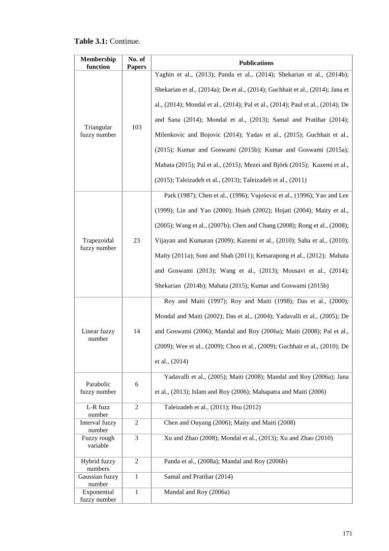
171


Membership

function

No. of

Papers Publications

Triangular

fuzzy number

103

Yaghin et al., (2013); Panda et al., (2014); Shekarian et al., (2014b);

Shekarian et al., (2014a); De et al., (2014); Guchhait et al., (2014); Jana et

al., (2014); Mondal et al., (2014); Pal et al., (2014); Paul et al., (2014); De

and Sana (2014); Mondal et al., (2013); Samal and Pratihar (2014);

Milenkovic and Bojovic (2014); Yadav et al., (2015); Guchhait et al.,

(2015); Kumar and Goswami (2015b); Kumar and Goswami (2015a);

Mahata (2015); Pal et al., (2015); Mezei and Björk (2015); Kazemi et al.,

(2015); Taleizadeh et al., (2013); Taleizadeh et al., (2011)

Trapezoidal

fuzzy number

23

Park (1987); Chen et al., (1996); Vujošević et al., (1996); Yao and Lee

(1999); Lin and Yao (2000); Hsieh (2002); Hojati (2004); Maity et al.,

(2005); Wang et al., (2007b); Chen and Chang (2008); Rong et al., (2008);

Vijayan and Kumaran (2009); Kazemi et al., (2010); Saha et al., (2010);

Maity (2011a); Soni and Shah (2011); Ketsarapong et al., (2012); Mahata

and Goswami (2013); Wang et al., (2013); Mousavi et al., (2014);

Shekarian (2014b); Mahata (2015); Kumar and Goswami (2015b)

Linear fuzzy

number

14

Roy and Maiti (1997); Roy and Maiti (1998); Das et al., (2000);

Mondal and Maiti (2002); Das et al., (2004); Yadavalli et al., (2005); De

and Goswami (2006); Mandal and Roy (2006a); Maiti (2008); Pal et al.,

(2009); Wee et al., (2009); Chou et al., (2009); Guchhait et al., (2010); De

et al., (2014)

Parabolic

fuzzy number

6

Yadavalli et al., (2005); Maiti (2008); Mandal and Roy (2006a); Jana

et al., (2013); Islam and Roy (2006); Mahapatra and Maiti (2006)

L-R fuzz

number

2 Taleizadeh et al., (2011); Hsu (2012)

Interval fuzzy

number

2 Chen and Ouyang (2006); Maity and Maiti (2008)

Fuzzy rough

variable

3 Xu and Zhao (2008); Mondal et al., (2013); Xu and Zhao (2010)

Hybrid fuzzy

numbers

2 Panda et al., (2008a); Mandal and Roy (2006b)

Gaussian fuzzy

number

1 Samal and Pratihar (2014)

Exponential

fuzzy number

1 Mandal and Roy (2006a)

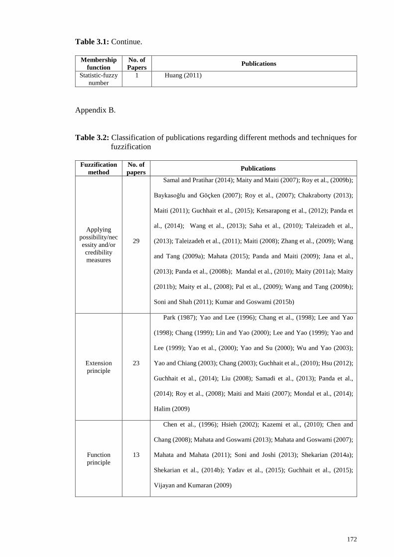
172


Membership

function

No. of

Papers Publications

Statistic-fuzzy

number

1 Huang (2011)

Appendix B.


fuzzification

Fuzzification

method

No. of

papers Publications

Applying

possibility/nec

essity and/or

credibility

measures

29

Samal and Pratihar (2014); Maity and Maiti (2007); Roy et al., (2009b);

Baykasoğlu and Göçken (2007); Roy et al., (2007); Chakraborty (2013);

Maiti (2011); Guchhait et al., (2015); Ketsarapong et al., (2012); Panda et

al., (2014); Wang et al., (2013); Saha et al., (2010); Taleizadeh et al.,

(2013); Taleizadeh et al., (2011); Maiti (2008); Zhang et al., (2009); Wang

and Tang (2009a); Mahata (2015); Panda and Maiti (2009); Jana et al.,

(2013); Panda et al., (2008b); Mandal et al., (2010); Maity (2011a); Maity

(2011b); Maity et al., (2008); Pal et al., (2009); Wang and Tang (2009b);

Soni and Shah (2011); Kumar and Goswami (2015b)

Extension

principle

23

Park (1987); Yao and Lee (1996); Chang et al., (1998); Lee and Yao

(1998); Chang (1999); Lin and Yao (2000); Lee and Yao (1999); Yao and

Lee (1999); Yao et al., (2000); Yao and Su (2000); Wu and Yao (2003);

Yao and Chiang (2003); Chang (2003); Guchhait et al., (2010); Hsu (2012);

Guchhait et al., (2014); Liu (2008); Samadi et al., (2013); Panda et al.,

(2014); Roy et al., (2008); Maiti and Maiti (2007); Mondal et al., (2014);

Halim (2009)

Function

principle

13

Chen et al., (1996); Hsieh (2002); Kazemi et al., (2010); Chen and

Chang (2008); Mahata and Goswami (2013); Mahata and Goswami (2007);

Mahata and Mahata (2011); Soni and Joshi (2013); Shekarian (2014a);

Shekarian et al., (2014b); Yadav et al., (2015); Guchhait et al., (2015);

Vijayan and Kumaran (2009)

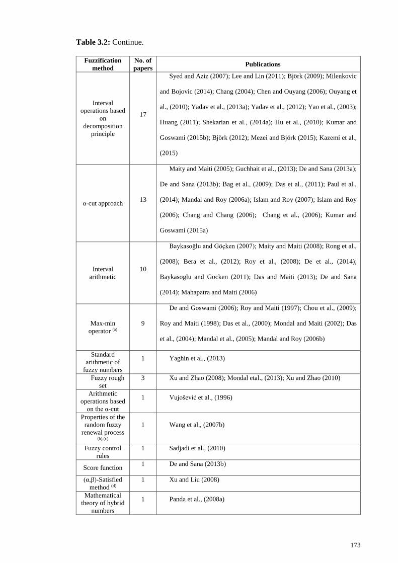
173


Fuzzification

method

No. of

papers Publications

Interval

operations based

on

decomposition

principle

17

Syed and Aziz (2007); Lee and Lin (2011); Björk (2009); Milenkovic

and Bojovic (2014); Chang (2004); Chen and Ouyang (2006); Ouyang et

al., (2010); Yadav et al., (2013a); Yadav et al., (2012); Yao et al., (2003);

Huang (2011); Shekarian et al., (2014a); Hu et al., (2010); Kumar and

Goswami (2015b); Björk (2012); Mezei and Björk (2015); Kazemi et al.,

(2015)

α-cut approach 13

Maity and Maiti (2005); Guchhait et al., (2013); De and Sana (2013a);

De and Sana (2013b); Bag et al., (2009); Das et al., (2011); Paul et al.,

(2014); Mandal and Roy (2006a); Islam and Roy (2007); Islam and Roy

(2006); Chang and Chang (2006); Chang et al., (2006); Kumar and

Goswami (2015a)

Interval

arithmetic

10

Baykasoğlu and Göçken (2007); Maity and Maiti (2008); Rong et al.,

(2008); Bera et al., (2012); Roy et al., (2008); De et al., (2014);

Baykasoglu and Gocken (2011); Das and Maiti (2013); De and Sana

(2014); Mahapatra and Maiti (2006)

Max-min

operator (a)

9

De and Goswami (2006); Roy and Maiti (1997); Chou et al., (2009);

Roy and Maiti (1998); Das et al., (2000); Mondal and Maiti (2002); Das

et al., (2004); Mandal et al., (2005); Mandal and Roy (2006b)

Standard

arithmetic of

fuzzy numbers

1 Yaghin et al., (2013)

Fuzzy rough

set

3 Xu and Zhao (2008); Mondal etal., (2013); Xu and Zhao (2010)

Arithmetic

operations based

on the α-cut

1 Vujošević et al., (1996)

Properties of the

random fuzzy

renewal process (b),(c)

1 Wang et al., (2007b)

Fuzzy control

rules

1 Sadjadi et al., (2010)

Score function 1 De and Sana (2013b)

(α,β)-Satisfied

method (d)

1 Xu and Liu (2008)

Mathematical

theory of hybrid

numbers

1 Panda et al., (2008a)

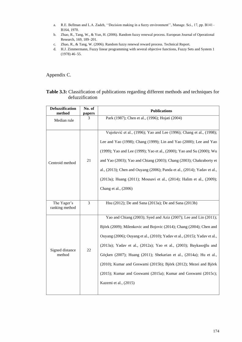
174

a. R.E. Bellman and L.A. Zadeh, ‘‘Decision making in a fuzzy environment’’, Manage. Sci., 17, pp. B141–

B164, 1970.

b. Zhao, R., Tang, W., & Yun, H. (2006). Random fuzzy renewal process. European Journal of Operational

Research, 169, 189–201.

c. Zhao, R., & Tang, W. (2006). Random fuzzy renewal reward process. Technical Report.

d. H.J. Zimmermann, Fuzzy linear programming with several objective functions, Fuzzy Sets and System 1

(1978) 46–55.

Appendix C.


defuzzification

Defuzzification

method

No. of

papers Publications

Median rule 3 Park (1987); Chen et al., (1996); Hojati (2004)

Centroid method 21

Vujošević et al., (1996); Yao and Lee (1996); Chang et al., (1998);

Lee and Yao (1998); Chang (1999); Lin and Yao (2000); Lee and Yao

(1999); Yao and Lee (1999); Yao et al., (2000); Yao and Su (2000); Wu

and Yao (2003); Yao and Chiang (2003); Chang (2003); Chakraborty et

al., (2013); Chen and Ouyang (2006); Panda et al., (2014); Yadav et al.,

(2013a); Huang (2011); Mousavi et al., (2014); Halim et al., (2009);

Chang et al., (2006)

The Yager’s

ranking method

3 Hsu (2012); De and Sana (2013a); De and Sana (2013b)

Signed distance

method

22

Yao and Chiang (2003); Syed and Aziz (2007); Lee and Lin (2011);

Björk (2009); Milenkovic and Bojovic (2014); Chang (2004); Chen and

Ouyang (2006); Ouyang et al., (2010); Yadav et al., (2015); Yadav et al.,

(2013a); Yadav et al., (2012a); Yao et al., (2003); Baykasoğlu and

Göçken (2007); Huang (2011); Shekarian et al., (2014a); Hu et al.,

(2010); Kumar and Goswami (2015b); Björk (2012); Mezei and Björk

(2015); Kumar and Goswami (2015a); Kumar and Goswami (2015c);

Kazemi et al., (2015)

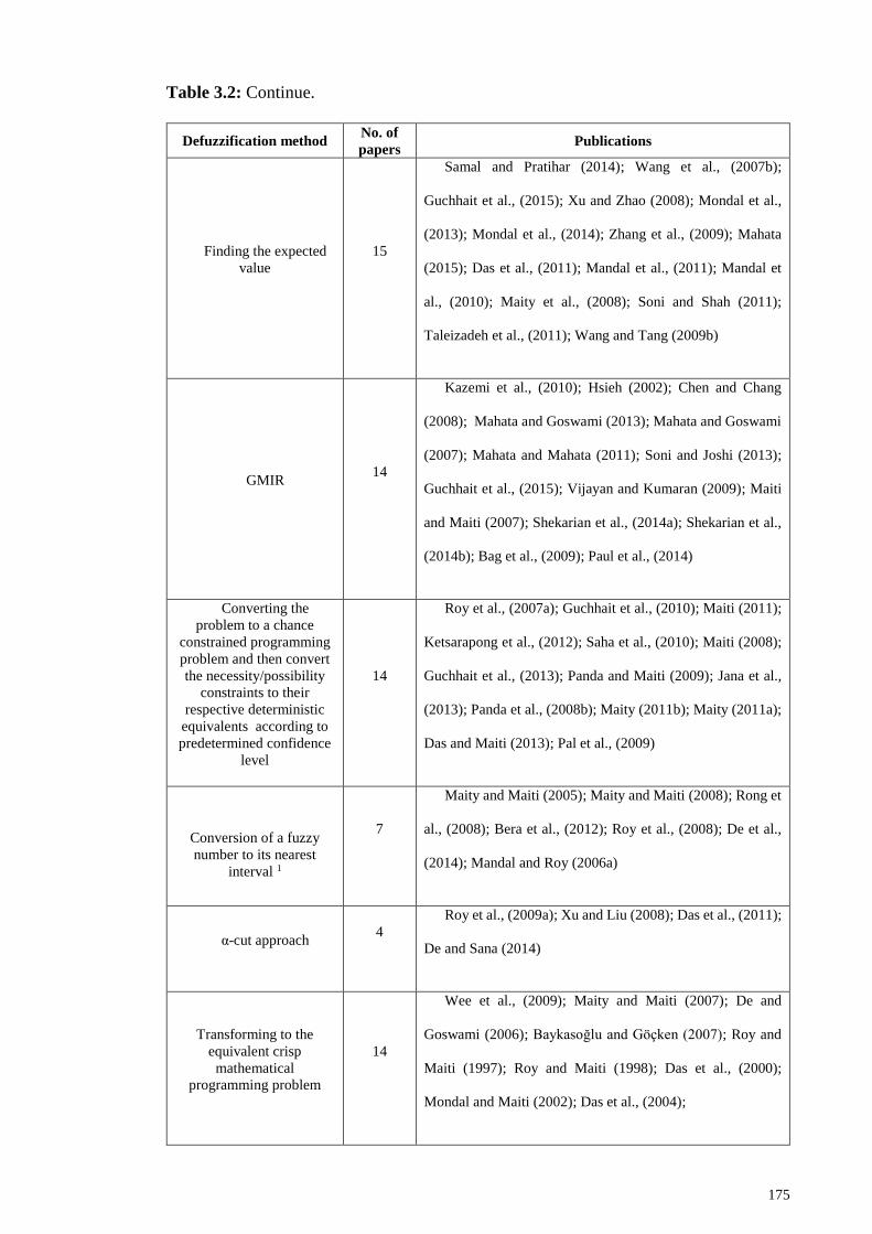
175


Defuzzification method No. of

papers Publications

Finding the expected

value

15

Samal and Pratihar (2014); Wang et al., (2007b);

Guchhait et al., (2015); Xu and Zhao (2008); Mondal et al.,

(2013); Mondal et al., (2014); Zhang et al., (2009); Mahata

(2015); Das et al., (2011); Mandal et al., (2011); Mandal et

al., (2010); Maity et al., (2008); Soni and Shah (2011);

Taleizadeh et al., (2011); Wang and Tang (2009b)

GMIR 14

Kazemi et al., (2010); Hsieh (2002); Chen and Chang

(2008); Mahata and Goswami (2013); Mahata and Goswami

(2007); Mahata and Mahata (2011); Soni and Joshi (2013);

Guchhait et al., (2015); Vijayan and Kumaran (2009); Maiti

and Maiti (2007); Shekarian et al., (2014a); Shekarian et al.,

(2014b); Bag et al., (2009); Paul et al., (2014)

Converting the

problem to a chance

constrained programming

problem and then convert

the necessity/possibility

constraints to their

respective deterministic

equivalents according to

predetermined confidence

level

14

Roy et al., (2007a); Guchhait et al., (2010); Maiti (2011);

Ketsarapong et al., (2012); Saha et al., (2010); Maiti (2008);

Guchhait et al., (2013); Panda and Maiti (2009); Jana et al.,

(2013); Panda et al., (2008b); Maity (2011b); Maity (2011a);

Das and Maiti (2013); Pal et al., (2009)

Conversion of a fuzzy

number to its nearest

interval 1

7

Maity and Maiti (2005); Maity and Maiti (2008); Rong et

al., (2008); Bera et al., (2012); Roy et al., (2008); De et al.,

(2014); Mandal and Roy (2006a)

α-cut approach 4

Roy et al., (2009a); Xu and Liu (2008); Das et al., (2011);

De and Sana (2014)

Transforming to the

equivalent crisp

mathematical

programming problem

14

Wee et al., (2009); Maity and Maiti (2007); De and

Goswami (2006); Baykasoğlu and Göçken (2007); Roy and

Maiti (1997); Roy and Maiti (1998); Das et al., (2000);

Mondal and Maiti (2002); Das et al., (2004);

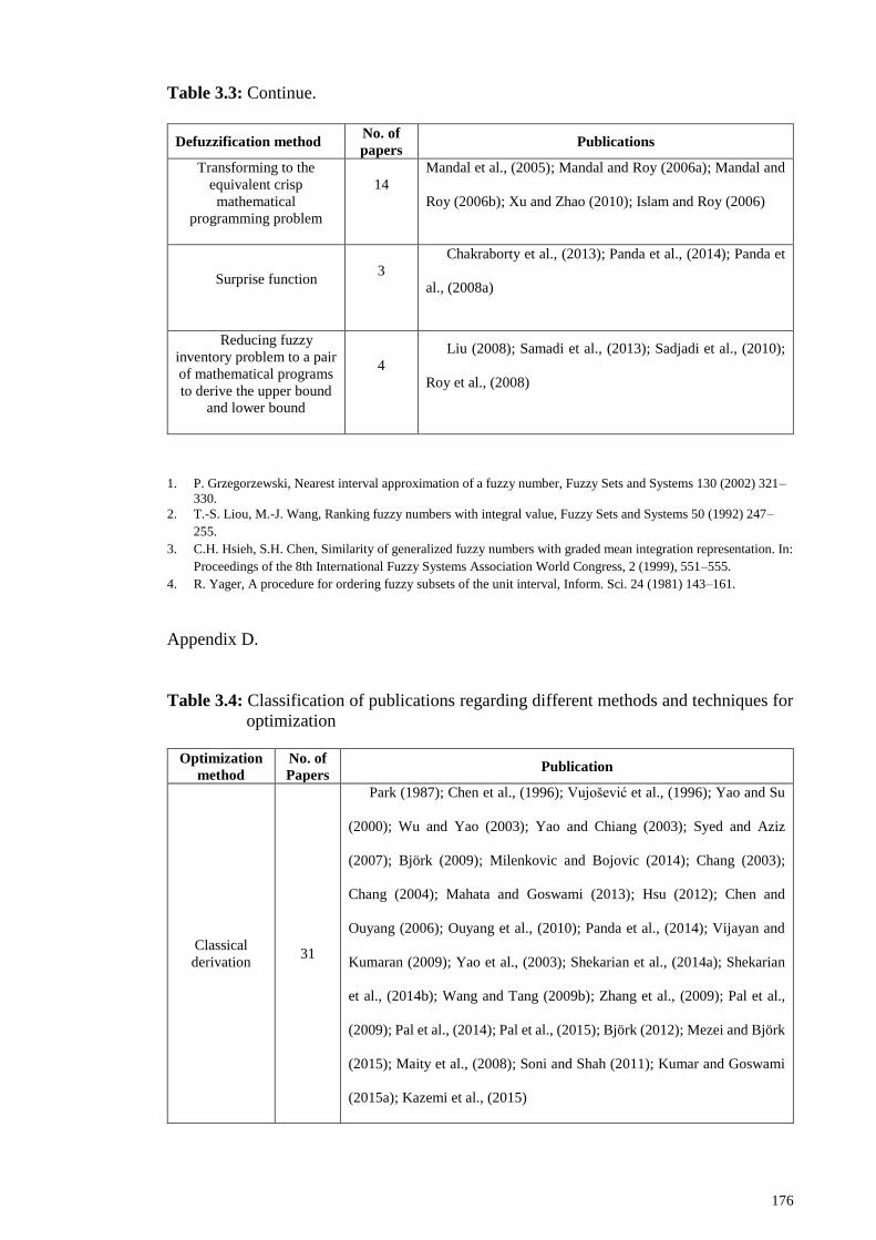
176


Defuzzification method No. of

papers Publications

Transforming to the

equivalent crisp

mathematical

programming problem

14

Mandal et al., (2005); Mandal and Roy (2006a); Mandal and

Roy (2006b); Xu and Zhao (2010); Islam and Roy (2006)

Surprise function 3

Chakraborty et al., (2013); Panda et al., (2014); Panda et

al., (2008a)

Reducing fuzzy

inventory problem to a pair

of mathematical programs

to derive the upper bound

and lower bound

4

Liu (2008); Samadi et al., (2013); Sadjadi et al., (2010);

Roy et al., (2008)

1. P. Grzegorzewski, Nearest interval approximation of a fuzzy number, Fuzzy Sets and Systems 130 (2002) 321–

330.

2. T.-S. Liou, M.-J. Wang, Ranking fuzzy numbers with integral value, Fuzzy Sets and Systems 50 (1992) 247–

255.

3. C.H. Hsieh, S.H. Chen, Similarity of generalized fuzzy numbers with graded mean integration representation. In:

Proceedings of the 8th International Fuzzy Systems Association World Congress, 2 (1999), 551–555.

4. R. Yager, A procedure for ordering fuzzy subsets of the unit interval, Inform. Sci. 24 (1981) 143–161.

Appendix D.


optimization

Optimization

method

No. of

Papers Publication

Classical

derivation 31

Park (1987); Chen et al., (1996); Vujošević et al., (1996); Yao and Su

(2000); Wu and Yao (2003); Yao and Chiang (2003); Syed and Aziz

(2007); Björk (2009); Milenkovic and Bojovic (2014); Chang (2003);

Chang (2004); Mahata and Goswami (2013); Hsu (2012); Chen and

Ouyang (2006); Ouyang et al., (2010); Panda et al., (2014); Vijayan and

Kumaran (2009); Yao et al., (2003); Shekarian et al., (2014a); Shekarian

et al., (2014b); Wang and Tang (2009b); Zhang et al., (2009); Pal et al.,

(2009); Pal et al., (2014); Pal et al., (2015); Björk (2012); Mezei and Björk

(2015); Maity et al., (2008); Soni and Shah (2011); Kumar and Goswami

(2015a); Kazemi et al., (2015)

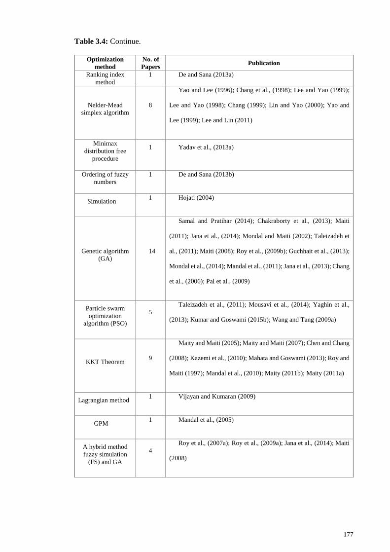
177


Optimization

method

No. of

Papers Publication

Ranking index

method

1 De and Sana (2013a)

Nelder-Mead

simplex algorithm

8

Yao and Lee (1996); Chang et al., (1998); Lee and Yao (1999);

Lee and Yao (1998); Chang (1999); Lin and Yao (2000); Yao and

Lee (1999); Lee and Lin (2011)

Minimax

distribution free

procedure

1 Yadav et al., (2013a)

Ordering of fuzzy

numbers

1 De and Sana (2013b)

Simulation 1 Hojati (2004)

Genetic algorithm

(GA)

14

Samal and Pratihar (2014); Chakraborty et al., (2013); Maiti

(2011); Jana et al., (2014); Mondal and Maiti (2002); Taleizadeh et

al., (2011); Maiti (2008); Roy et al., (2009b); Guchhait et al., (2013);

Mondal et al., (2014); Mandal et al., (2011); Jana et al., (2013); Chang

et al., (2006); Pal et al., (2009)

Particle swarm

optimization

algorithm (PSO)

5

Taleizadeh et al., (2011); Mousavi et al., (2014); Yaghin et al.,

(2013); Kumar and Goswami (2015b); Wang and Tang (2009a)

KKT Theorem 9

Maity and Maiti (2005); Maity and Maiti (2007); Chen and Chang

(2008); Kazemi et al., (2010); Mahata and Goswami (2013); Roy and

Maiti (1997); Mandal et al., (2010); Maity (2011b); Maity (2011a)

Lagrangian method 1 Vijayan and Kumaran (2009)

GPM 1 Mandal et al., (2005)

A hybrid method

fuzzy simulation

(FS) and GA

4

Roy et al., (2007a); Roy et al., (2009a); Jana et al., (2014); Maiti

(2008)

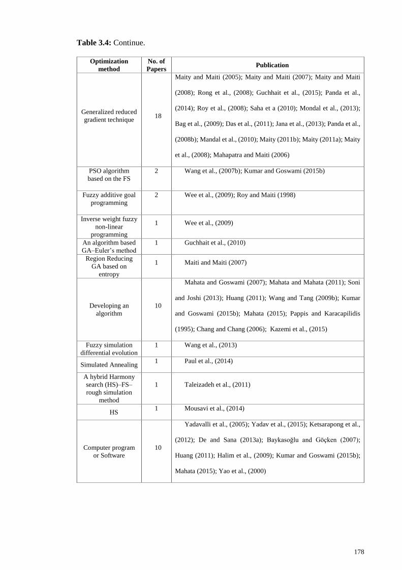
178


Optimization

method

No. of

Papers Publication

Generalized reduced

gradient technique 18

Maity and Maiti (2005); Maity and Maiti (2007); Maity and Maiti

(2008); Rong et al., (2008); Guchhait et al., (2015); Panda et al.,

(2014); Roy et al., (2008); Saha et a (2010); Mondal et al., (2013);

Bag et al., (2009); Das et al., (2011); Jana et al., (2013); Panda et al.,

(2008b); Mandal et al., (2010); Maity (2011b); Maity (2011a); Maity

et al., (2008); Mahapatra and Maiti (2006)

PSO algorithm

based on the FS

2 Wang et al., (2007b); Kumar and Goswami (2015b)

Fuzzy additive goal

programming

2 Wee et al., (2009); Roy and Maiti (1998)

Inverse weight fuzzy

non-linear

programming

1 Wee et al., (2009)

An algorithm based

GA–Euler’s method

1 Guchhait et al., (2010)

Region Reducing

GA based on

entropy

1 Maiti and Maiti (2007)

Developing an

algorithm

10

Mahata and Goswami (2007); Mahata and Mahata (2011); Soni

and Joshi (2013); Huang (2011); Wang and Tang (2009b); Kumar

and Goswami (2015b); Mahata (2015); Pappis and Karacapilidis

(1995); Chang and Chang (2006); Kazemi et al., (2015)

Fuzzy simulation

differential evolution

1 Wang et al., (2013)

Simulated Annealing 1 Paul et al., (2014)

A hybrid Harmony

search (HS)–FS–

rough simulation

method

1 Taleizadeh et al., (2011)

HS 1 Mousavi et al., (2014)

Computer program

or Software

10

Yadavalli et al., (2005); Yadav et al., (2015); Ketsarapong et al.,

(2012); De and Sana (2013a); Baykasoğlu and Göçken (2007);

Huang (2011); Halim et al., (2009); Kumar and Goswami (2015b);

Mahata (2015); Yao et al., (2000)

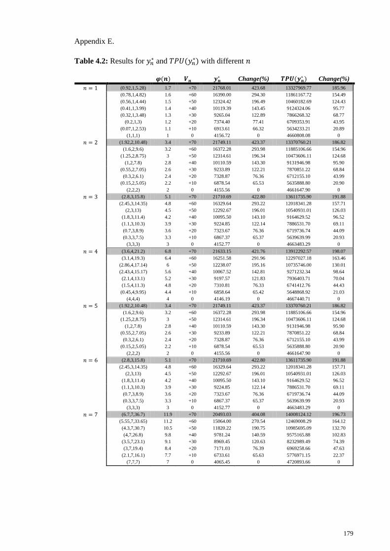
179

Appendix E.

Table 4.2: Results for 𝑦𝑛∗ and 𝑇𝑃𝑈(𝑦𝑛

∗) with different 𝑛

𝝋(𝒏) 𝑽𝒏 𝒚𝒏∗ Change(%) 𝑻𝑷𝑼(𝒚𝒏

∗ ) Change(%)

𝑛 = 1 (0.92,1,5.28) 1.7 +70 21768.01 423.68 13327969.77 185.96

(0.78,1,4.82) 1.6 +60 16390.00 294.30 11861167.72 154.49

(0.56,1,4.44) 1.5 +50 12324.42 196.49 10460182.69 124.43

(0.41,1,3.99) 1.4 +40 10119.39 143.45 9124324.06 95.77

(0.32,1,3.48) 1.3 +30 9265.04 122.89 7866268.32 68.77

(0.2,1,3) 1.2 +20 7374.40 77.41 6709353.91 43.95

(0.07,1,2.53) 1.1 +10 6913.61 66.32 5634233.21 20.89

(1,1,1) 1 0 4156.72 0 4660808.08 0

𝑛 = 2 (1.92,2,10.48) 3.4 +70 21749.11 423.37 13370760.21 186.82

(1.6,2,9.6) 3.2 +60 16372.28 293.98 11885106.66 154.96

(1.25,2,8.75) 3 +50 12314.61 196.34 10473606.11 124.68

(1,2,7.8) 2.8 +40 10110.59 143.30 9131946.98 95.90

(0.55,2,7.05) 2.6 +30 9233.89 122.21 7870851.22 68.84

(0.3,2,6.1) 2.4 +20 7328.87 76.36 6712155.10 43.99

(0.15,2,5.05) 2.2 +10 6878.54 65.53 5635888.80 20.90

(2,2,2) 2 0 4155.56 0 4661647.90 0

𝑛 = 3 (2.8,3,15.8) 5.1 +70 21710.69 422.80 13611735.90 191.88

(2.45,3,14.35) 4.8 +60 16329.64 293.22 12018341.28 157.71

(2,3,13) 4.5 +50 12292.67 196.01 10540931.01 126.03

(1.8,3,11.4) 4.2 +40 10095.50 143.10 9164629.52 96.52

(1.1,3,10.3) 3.9 +30 9224.85 122.14 7886531.70 69.11

(0.7,3,8.9) 3.6 +20 7323.67 76.36 6719736.74 44.09

(0.3,3,7.5) 3.3 +10 6867.37 65.37 5639639.99 20.93

(3,3,3) 3 0 4152.77 0 4663483.29 0

𝑛 = 4 (3.6,4,21.2) 6.8 +70 21633.15 421.76 13912292.57 198.07

(3.1,4,19.3) 6.4 +60 16251.58 291.96 12297027.18 163.46

(2.86,4,17.14) 6 +50 12238.07 195.16 10735746.00 130.01

(2.43,4,15.17) 5.6 +40 10067.52 142.81 9271232.34 98.64

(2.1,4,13.1) 5.2 +30 9197.57 121.83 7936403.71 70.04

(1.5,4,11.3) 4.8 +20 7310.81 76.33 6741412.76 44.43

(0.45,4,9.95) 4.4 +10 6858.64 65.42 5648868.92 21.03

(4,4,4) 4 0 4146.19 0 4667440.71 0

𝑛 = 5 (1.92,2,10.48) 3.4 +70 21749.11 423.37 13370760.21 186.82

(1.6,2,9.6) 3.2 +60 16372.28 293.98 11885106.66 154.96

(1.25,2,8.75) 3 +50 12314.61 196.34 10473606.11 124.68

(1,2,7.8) 2.8 +40 10110.59 143.30 9131946.98 95.90

(0.55,2,7.05) 2.6 +30 9233.89 122.21 7870851.22 68.84

(0.3,2,6.1) 2.4 +20 7328.87 76.36 6712155.10 43.99

(0.15,2,5.05) 2.2 +10 6878.54 65.53 5635888.80 20.90

(2,2,2) 2 0 4155.56 0 4661647.90 0

𝑛 = 6 (2.8,3,15.8) 5.1 +70 21710.69 422.80 13611735.90 191.88

(2.45,3,14.35) 4.8 +60 16329.64 293.22 12018341.28 157.71

(2,3,13) 4.5 +50 12292.67 196.01 10540931.01 126.03

(1.8,3,11.4) 4.2 +40 10095.50 143.10 9164629.52 96.52

(1.1,3,10.3) 3.9 +30 9224.85 122.14 7886531.70 69.11

(0.7,3,8.9) 3.6 +20 7323.67 76.36 6719736.74 44.09

(0.3,3,7.5) 3.3 +10 6867.37 65.37 5639639.99 20.93

(3,3,3) 3 0 4152.77 0 4663483.29 0

𝑛 = 7 (6.7,7,36.7) 11.9 +70 20493.03 404.08 14008124.12 196.73

(5.55,7,33.65) 11.2 +60 15064.00 270.54 12469008.29 164.12

(4.3,7,30.7) 10.5 +50 11820.22 190.75 10985695.09 132.70

(4,7,26.8) 9.8 +40 9781.24 140.59 9575165.88 102.83

(3.5,7,23.1) 9.1 +30 8969.45 120.63 8232989.49 74.39

(3,7,19.4) 8.4 +20 7171.03 76.39 6969258.66 47.63

(2.1,7,16.1) 7.7 +10 6733.61 65.63 5776971.15 22.37

(7,7,7) 7 0 4065.45 0 4720893.66 0

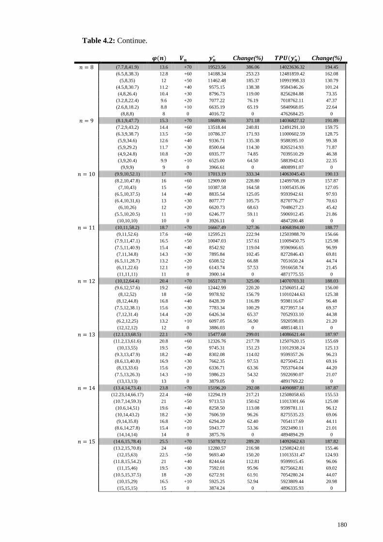
180



∗ ) Change(%)

𝑛 = 8 (7.7,8,41.9) 13.6 +70 19523.56 386.06 14023636.32 194.45

(6.5,8,38.3) 12.8 +60 14188.34 253.23 12481859.42 162.08

(5,8,35) 12 +50 11462.48 185.37 10991998.33 130.79

(4.5,8,30.7) 11.2 +40 9575.15 138.38 9584346.26 101.24

(4,8,26.4) 10.4 +30 8796.73 119.00 8256284.88 73.35

(3.2,8,22.4) 9.6 +20 7077.22 76.19 7018762.11 47.37

(2.6,8,18.2) 8.8 +10 6635.19 65.19 5840968.05 22.64

(8,8,8) 8 0 4016.72 0 4762684.25 0

𝑛 = 9 (8.1,9,47.7) 15.3 +70 18689.86 371.18 14036827.12 191.89

(7.2,9,43.2) 14.4 +60 13518.44 240.81 12491291.10 159.75

(6.3,9,38.7) 13.5 +50 10786.37 171.93 11000602.59 128.75

(5,9,34.6) 12.6 +40 9336.71 135.38 9588395.10 99.38

(5,9,29.2) 11.7 +30 8500.64 114.30 8265214.93 71.87

(4,9,24.8) 10.8 +20 6935.77 74.85 7039510.29 46.38

(3,9,20.4) 9.9 +10 6525.00 64.50 5883942.43 22.35

(9,9,9) 9 0 3966.61 0 4808991.07 0

𝑛 = 10 (9.9,10,52.1) 17 +70 17013.19 333.34 14063045.43 190.13

(8.2,10,47.8) 16 +60 12909.00 228.80 12499708.19 157.87

(7,10,43) 15 +50 10387.58 164.58 11005435.06 127.05

(6.5,10,37.5) 14 +40 8835.54 125.05 9593942.61 97.93

(6.4,10,31,6) 13 +30 8077.77 105.75 8270776.27 70.63

(6,10,26) 12 +20 6620.73 68.63 7048627.23 45.42

(5.5,10,20.5) 11 +10 6246.77 59.11 5906912.45 21.86

(10,10,10) 10 0 3926.11 0 4847200.48 0

𝑛 = 11 (10,11,58.2) 18.7 +70 16667.49 327.36 14068394.00 188.77

(9,11,52.6) 17.6 +60 12595.21 222.94 12503988.70 156.66

(7.9,11,47.1) 16.5 +50 10047.03 157.61 11009450.75 125.98

(7.5,11,40.9) 15.4 +40 8542.92 119.04 9596966.65 96.99

(7,11,34.8) 14.3 +30 7895.84 102.45 8272846.43 69.81

(6.5,11,28.7) 13.2 +20 6508.52 66.88 7051650.24 44.74

(6,11,22.6) 12.1 +10 6143.74 57.53 5916658.74 21.45

(11,11,11) 11 0 3900.14 0 4871775.55 0

𝑛 = 12 (10,12,64.4) 20.4 +70 16517.78 325.06 14070703.31 188.03

(9.6,12,57.6) 19.2 +60 12442.99 220.20 12506051.42 156.00

(8,12,52) 18 +50 9978.92 156.79 11010244.63 125.38

(8,12,44.8) 16.8 +40 8428.39 116.89 9598116.67 96.48

(7.5,12,38.1) 15.6 +30 7783.34 100.29 8273957.14 69.37

(7,12,31.4) 14.4 +20 6426.34 65.37 7052933.10 44.38

(6.2,12,25) 13.2 +10 6097.05 56.90 5920598.03 21.20

(12,12,12) 12 0 3886.03 0 4885148.11 0

𝑛 = 13 (12.1,13,68.5) 22.1 +70 15477.68 299.01 14086621.44 187.97

(11.2,13,61.6) 20.8 +60 12326.76 217.78 12507620.15 155.69

(10,13,55) 19.5 +50 9745.31 151.23 11012938.24 125.13

(9.3,13,47.9) 18.2 +40 8302.08 114.02 9599357.26 96.23

(8.6,13,40.8) 16.9 +30 7662.35 97.53 8275045.21 69.16

(8,13,33.6) 15.6 +20 6336.71 63.36 7053764.04 44.20

(7.5,13,26.3) 14.3 +10 5986.23 54.32 5922690.07 21.07

(13,13,13) 13 0 3879.05 0 4891769.22 0

𝑛 = 14 (13.4,14,73.4) 23.8 +70 15196.20 292.08 14090887.81 187.87

(12.23,14,66.17) 22.4 +60 12294.19 217.21 12508058.65 155.53

(10.7,14,59.3) 21 +50 9713.53 150.62 11013301.66 125.00

(10.6,14,51) 19.6 +40 8258.50 113.08 9599781.11 96.12

(10,14,43.2) 18.2 +30 7606.59 96.26 8275535.23 69.06

(9,14,35.8) 16.8 +20 6294.20 62.40 7054117.69 44.11

(8.6,14,27.8) 15.4 +10 5943.77 53.36 5923490.11 21.01

(14,14,14) 14 0 3875.76 0 4894894.29 0

𝑛 = 15 (14.6,15,78.4) 25.5 +70 15078.72 289.20 14092662.63 187.82

(13.2,15,70.8) 24 +60 12280.57 216.98 12508242.01 155.46

(12,15,63) 22.5 +50 9693.40 150.20 11013531.47 124.93

(11.8,15,54.2) 21 +40 8244.64 112.81 9599915.45 96.06

(11,15,46) 19.5 +30 7592.01 95.96 8275662.81 69.02

(10.5,15,37.5) 18 +20 6272.91 61.91 7054280.24 44.07

(10,15,29) 16.5 +10 5925.25 52.94 5923809.44 20.98

(15,15,15) 15 0 3874.24 0 4896335.93 0

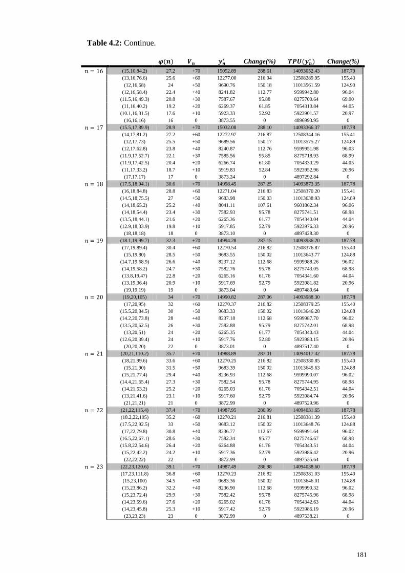
181



∗ ) Change(%)

𝑛 = 16 (15,16,84.2) 27.2 +70 15052.89 288.61 14093052.43 187.79

(13,16,76.6) 25.6 +60 12277.00 216.94 12508289.95 155.43

(12,16,68) 24 +50 9690.76 150.18 11013561.59 124.90

(12,16,58.4) 22.4 +40 8241.82 112.77 9599942.80 96.04

(11.5,16,49.3) 20.8 +30 7587.67 95.88 8275700.64 69.00

(11,16,40.2) 19.2 +20 6269.37 61.85 7054310.84 44.05

(10.1,16,31.5) 17.6 +10 5923.33 52.92 5923901.57 20.97

(16,16,16) 16 0 3873.55 0 4896993.95 0

𝑛 = 17 (15.5,17,89.9) 28.9 +70 15032.08 288.10 14093366.37 187.78

(14,17,81.2) 27.2 +60 12272.97 216.87 12508344.16 155.41

(12,17,73) 25.5 +50 9689.56 150.17 11013575.27 124.89

(12,17,62.8) 23.8 +40 8240.87 112.76 9599951.98 96.03

(11.9,17,52.7) 22.1 +30 7585.56 95.85 8275718.93 68.99

(11.9,17,42.5) 20.4 +20 6266.74 61.80 7054330.29 44.05

(11,17,33.2) 18.7 +10 5919.83 52.84 5923952.96 20.96

(17,17,17) 17 0 3873.24 0 4897292.84 0

𝑛 = 18 (17.5,18,94.1) 30.6 +70 14998.45 287.25 14093873.35 187.78

(16,18,84.8) 28.8 +60 12271.04 216.83 12508370.20 155.41

(14.5,18,75.5) 27 +50 9683.98 150.03 11013638.93 124.89

(14,18,65.2) 25.2 +40 8041.11 107.61 9601862.34 96.06

(14,18,54.4) 23.4 +30 7582.93 95.78 8275741.51 68.98

(13.5,18,44.1) 21.6 +20 6265.36 61.77 7054340.04 44.04

(12.9,18,33.9) 19.8 +10 5917.85 52.79 5923976.33 20.96

(18,18,18) 18 0 3873.10 0 4897428.30 0

𝑛 = 19 (18.1,19,99.7) 32.3 +70 14994.28 287.15 14093936.20 187.78

(17,19,89.4) 30.4 +60 12270.54 216.82 12508376.87 155.40

(15,19,80) 28.5 +50 9683.55 150.02 11013643.77 124.88

(14.7,19,68.9) 26.6 +40 8237.12 112.68 9599988.26 96.02

(14,19,58.2) 24.7 +30 7582.76 95.78 8275743.05 68.98

(13.8,19,47) 22.8 +20 6265.16 61.76 7054341.60 44.04

(13,19,36.4) 20.9 +10 5917.69 52.79 5923981.82 20.96

(19,19,19) 19 0 3873.04 0 4897489.64 0

𝑛 = 20 (19,20,105) 34 +70 14990.82 287.06 14093988.30 187.78

(17,20,95) 32 +60 12270.37 216.82 12508379.25 155.40

(15.5,20,84.5) 30 +50 9683.33 150.02 11013646.28 124.88

(14.2,20,73.8) 28 +40 8237.18 112.68 9599987.70 96.02

(13.5,20,62.5) 26 +30 7582.88 95.79 8275742.01 68.98

(13,20,51) 24 +20 6265.35 61.77 7054340.43 44.04

(12.6,20,39.4) 24 +10 5917.76 52.80 5923983.15 20.96

(20,20,20) 22 0 3873.01 0 4897517.40 0

𝑛 = 21 (20,21,110.2) 35.7 +70 14988.89 287.01 14094017.42 187.78

(18,21,99.6) 33.6 +60 12270.25 216.82 12508380.85 155.40

(15,21,90) 31.5 +50 9683.39 150.02 11013645.63 124.88

(15,21,77.4) 29.4 +40 8236.93 112.68 9599990.07 96.02

(14.4,21,65.4) 27.3 +30 7582.54 95.78 8275744.95 68.98

(14,21,53.2) 25.2 +20 6265.03 61.76 7054342.51 44.04

(13,21,41.6) 23.1 +10 5917.60 52.79 5923984.74 20.96

(21,21,21) 21 0 3872.99 0 4897529.96 0

𝑛 = 22 (21,22,115.4) 37.4 +70 14987.95 286.99 14094031.65 187.78

(18.2,22,105) 35.2 +60 12270.21 216.81 12508381.39 155.40

(17.5,22,92.5) 33 +50 9683.12 150.02 11013648.76 124.88

(17,22,79.8) 30.8 +40 8236.77 112.67 9599991.64 96.02

(16.5,22,67.1) 28.6 +30 7582.34 95.77 8275746.67 68.98

(15.8,22,54.6) 26.4 +20 6264.88 61.76 7054343.51 44.04

(15,22,42.2) 24.2 +10 5917.36 52.79 5923986.42 20.96

(22,22,22) 22 0 3872.99 0 4897535.64 0

𝑛 = 23 (22,23,120.6) 39.1 +70 14987.49 286.98 14094038.60 187.78

(17,23,111.8) 36.8 +60 12270.23 216.82 12508381.03 155.40

(15,23,100) 34.5 +50 9683.36 150.02 11013646.01 124.88

(15,23,86.2) 32.2 +40 8236.90 112.68 9599990.32 96.02

(15,23,72.4) 29.9 +30 7582.42 95.78 8275745.96 68.98

(14,23,59.6) 27.6 +20 6265.02 61.76 7054342.63 44.04

(14,23,45.8) 25.3 +10 5917.42 52.79 5923986.19 20.96

(23,23,23) 23 0 3872.99 0 4897538.21 0

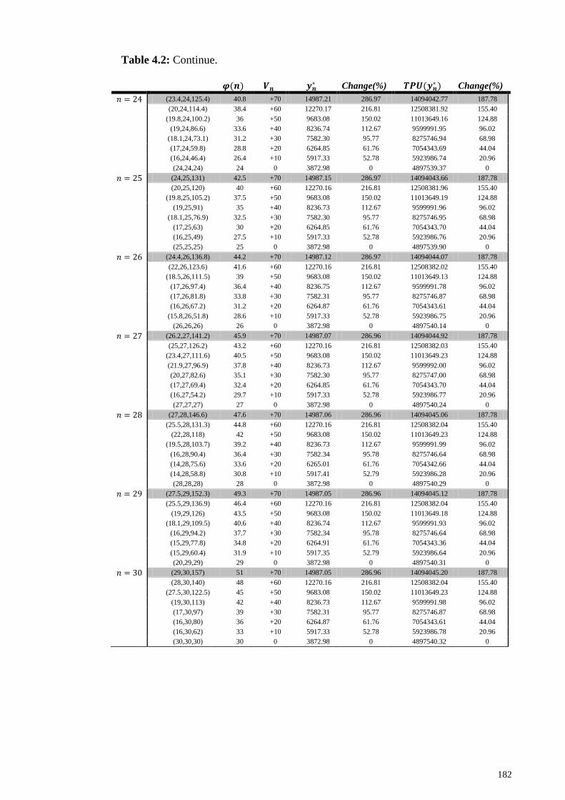
182



∗ ) Change(%)

𝑛 = 24 (23.4,24,125.4) 40.8 +70 14987.21 286.97 14094042.77 187.78

(20,24,114.4) 38.4 +60 12270.17 216.81 12508381.92 155.40

(19.8,24,100.2) 36 +50 9683.08 150.02 11013649.16 124.88

(19,24,86.6) 33.6 +40 8236.74 112.67 9599991.95 96.02

(18.1,24,73.1) 31.2 +30 7582.30 95.77 8275746.94 68.98

(17,24,59.8) 28.8 +20 6264.85 61.76 7054343.69 44.04

(16,24,46.4) 26.4 +10 5917.33 52.78 5923986.74 20.96

(24,24,24) 24 0 3872.98 0 4897539.37 0

𝑛 = 25 (24,25,131) 42.5 +70 14987.15 286.97 14094043.66 187.78

(20,25,120) 40 +60 12270.16 216.81 12508381.96 155.40

(19.8,25,105.2) 37.5 +50 9683.08 150.02 11013649.19 124.88

(19,25,91) 35 +40 8236.73 112.67 9599991.96 96.02

(18.1,25,76.9) 32.5 +30 7582.30 95.77 8275746.95 68.98

(17,25,63) 30 +20 6264.85 61.76 7054343.70 44.04

(16,25,49) 27.5 +10 5917.33 52.78 5923986.76 20.96

(25,25,25) 25 0 3872.98 0 4897539.90 0

𝑛 = 26 (24.4,26,136.8) 44.2 +70 14987.12 286.97 14094044.07 187.78

(22,26,123.6) 41.6 +60 12270.16 216.81 12508382.02 155.40

(18.5,26,111.5) 39 +50 9683.08 150.02 11013649.13 124.88

(17,26,97.4) 36.4 +40 8236.75 112.67 9599991.78 96.02

(17,26,81.8) 33.8 +30 7582.31 95.77 8275746.87 68.98

(16,26,67.2) 31.2 +20 6264.87 61.76 7054343.61 44.04

(15.8,26,51.8) 28.6 +10 5917.33 52.78 5923986.75 20.96

(26,26,26) 26 0 3872.98 0 4897540.14 0

𝑛 = 27 (26.2,27,141.2) 45.9 +70 14987.07 286.96 14094044.92 187.78

(25,27,126.2) 43.2 +60 12270.16 216.81 12508382.03 155.40

(23.4,27,111.6) 40.5 +50 9683.08 150.02 11013649.23 124.88

(21.9,27,96.9) 37.8 +40 8236.73 112.67 9599992.00 96.02

(20,27,82.6) 35.1 +30 7582.30 95.77 8275747.00 68.98

(17,27,69.4) 32.4 +20 6264.85 61.76 7054343.70 44.04

(16,27,54.2) 29.7 +10 5917.33 52.78 5923986.77 20.96

(27,27,27) 27 0 3872.98 0 4897540.24 0

𝑛 = 28 (27,28,146.6) 47.6 +70 14987.06 286.96 14094045.06 187.78

(25.5,28,131.3) 44.8 +60 12270.16 216.81 12508382.04 155.40

(22,28,118) 42 +50 9683.08 150.02 11013649.23 124.88

(19.5,28,103.7) 39.2 +40 8236.73 112.67 9599991.99 96.02

(16,28,90.4) 36.4 +30 7582.34 95.78 8275746.64 68.98

(14,28,75.6) 33.6 +20 6265.01 61.76 7054342.66 44.04

(14,28,58.8) 30.8 +10 5917.41 52.79 5923986.28 20.96

(28,28,28) 28 0 3872.98 0 4897540.29 0

𝑛 = 29 (27.5,29,152.3) 49.3 +70 14987.05 286.96 14094045.12 187.78

(25.5,29,136.9) 46.4 +60 12270.16 216.81 12508382.04 155.40

(19,29,126) 43.5 +50 9683.08 150.02 11013649.18 124.88

(18.1,29,109.5) 40.6 +40 8236.74 112.67 9599991.93 96.02

(16,29,94.2) 37.7 +30 7582.34 95.78 8275746.64 68.98

(15,29,77.8) 34.8 +20 6264.91 61.76 7054343.36 44.04

(15,29,60.4) 31.9 +10 5917.35 52.79 5923986.64 20.96

(20,29,29) 29 0 3872.98 0 4897540.31 0

𝑛 = 30 (29,30,157) 51 +70 14987.05 286.96 14094045.20 187.78

(28,30,140) 48 +60 12270.16 216.81 12508382.04 155.40

(27.5,30,122.5) 45 +50 9683.08 150.02 11013649.23 124.88

(19,30,113) 42 +40 8236.73 112.67 9599991.98 96.02

(17,30,97) 39 +30 7582.31 95.77 8275746.87 68.98

(16,30,80) 36 +20 6264.87 61.76 7054343.61 44.04

(16,30,62) 33 +10 5917.33 52.78 5923986.78 20.96

(30,30,30) 30 0 3872.98 0 4897540.32 0

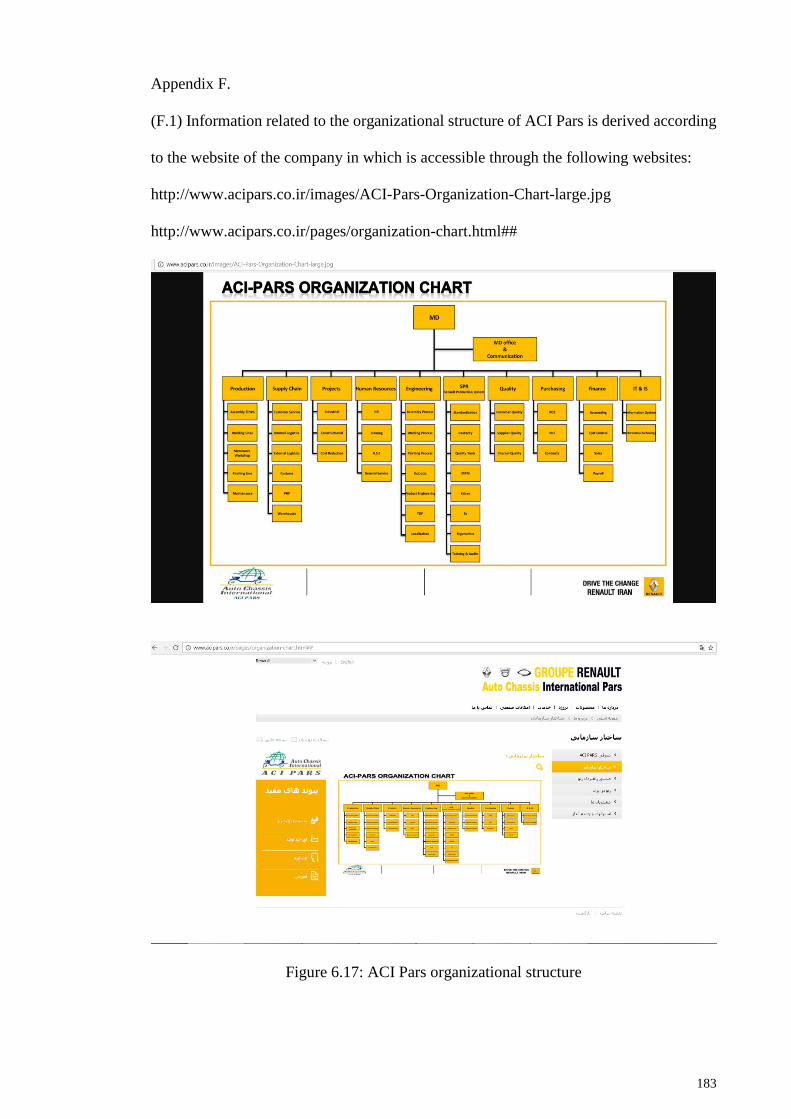
183

Appendix F.

(F.1) Information related to the organizational structure of ACI Pars is derived according

to the website of the company in which is accessible through the following websites:

http://www.acipars.co.ir/images/ACI-Pars-Organization-Chart-large.jpg

http://www.acipars.co.ir/pages/organization-chart.html##

Figure 6.17: ACI Pars organizational structure

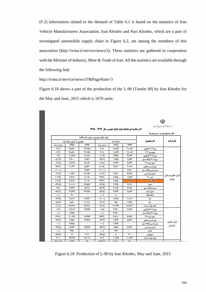
184

(F.2) Information related to the demand of Table 6.1 is based on the statistics of Iran

Vehicle Manufacturers Association. Iran Khodro and Pars Khodro, which are a part of

investigated automobile supply chain in Figure 6.2, are among the members of this

association (http://ivma.ir/service/news/3). These statistics are gathered in cooperation

with the Minister of Industry, Mine & Trade of Iran. All the statistics are available through

the following link:

http://ivma.ir/service/news/3?&PageNum=3

Figure 6.18 shows a part of the production of the L-90 (Tondar 90) by Iran Khodro for

the May and June, 2015 which is 1676 units.

Figure 6.18: Production of L-90 by Iran Khodro, May and June, 2015

185

(F.3) In Table 6.8 and 6.9, selling price of good quality Brake Disc and Rear Hub Drum

items are derived according to the price announced by Saipa After Sale Services

Organization that is working with Pars Khodro. Figure 6.19 shows the price of Brake

Disc among the other parts of braking system of L90. It should be mentioned that the

derived prices were modified based on the rate of inflation. These information can be

accessible through the website of this organization: http://www.saipayadak.org/470.

Figure 6.19: Price of some parts of braking system of L90

Tables 6.4-6.7 and Tables 6.10-6.15 are provided based on the dealerships of Iran Khodro

who are involving in selling and repairing L90. List of them is accessible through

http://www.ikco.ir/fa/Dealers.aspx.

(F.4) In order to derive the demand of containers, related statistics of production of milk

in Hamedan province reported by Statistical Center of Iran were used. These reports can

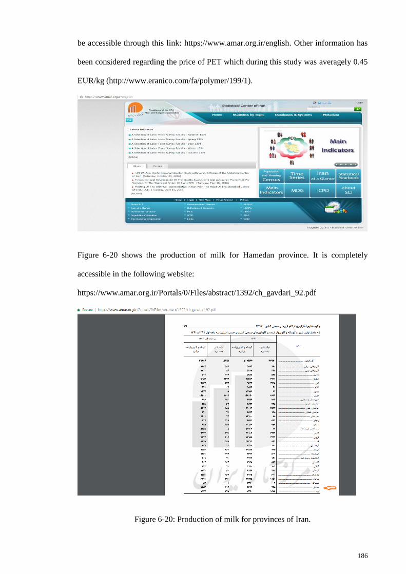
186

be accessible through this link: https://www.amar.org.ir/english. Other information has

been considered regarding the price of PET which during this study was averagely 0.45

EUR/kg (http://www.eranico.com/fa/polymer/199/1).

Figure 6-20 shows the production of milk for Hamedan province. It is completely

accessible in the following website:

https://www.amar.org.ir/Portals/0/Files/abstract/1392/ch_gavdari_92.pdf

Figure 6-20: Production of milk for provinces of Iran.

FORWARD AND BACKWARD FUZZY ECONOMIC ORDER...

Documents

Transcript of FORWARD AND BACKWARD FUZZY ECONOMIC ORDER...