Formal sequential equivalence checking of digital systems ...

HAL Id: tel-00163429https://tel.archives-ouvertes.fr/tel-00163429

Submitted on 17 Jul 2007

HAL is a multi-disciplinary open accessarchive for the deposit and dissemination of sci-entific research documents, whether they are pub-lished or not. The documents may come fromteaching and research institutions in France orabroad, or from public or private research centers.

L’archive ouverte pluridisciplinaire HAL, estdestinée au dépôt et à la diffusion de documentsscientifiques de niveau recherche, publiés ou non,émanant des établissements d’enseignement et derecherche français ou étrangers, des laboratoirespublics ou privés.

Formal sequential equivalence checking of digitalsystems by symbolic simulation

G. Ritter

To cite this version:G. Ritter. Formal sequential equivalence checking of digital systems by symbolic simulation. Microand nanotechnologies/Microelectronics. Université Joseph-Fourier - Grenoble I, 2001. English. �tel-00163429�

https://tel.archives-ouvertes.fr/tel-00163429

https://hal.archives-ouvertes.fr

Formal Sequential Equivalence Checking of

Digital Systems by Symbolic Simulation

A Dissertation submitted to

Fachbereich 18

Darmstadt University of Technology

Germany

Universite Joseph Fourier

Grenoble I

France

to obtain the bi-national degree (Co-tutelle de these)∗ of

Doctor in Electrical Engineering

Gerd RITTER

Jury

President: Prof. H. L. Hartnagel

Thesis Supervisors: Prof. D. Borrione

Prof. H. Eveking

Jury Members: Prof. P. Bakowski

Prof. M. Glesner

Day of submission: 21.12.2000

Day of defense: 26.03.2001

Research performed at

Dept. of Electrical and

Computer Engineering


TIMA Laboratory


Grenoble

∗ arrete ministeriel du 5 Juillet 1984, du 23 Novembre 1988 et du 18 Janvier 1994

Contents

1 Introduction 1

2 Overview of the Symbolic Simulation Approach 3

2.1 Principles of Symbolic Simulation . . . . . . . . . . . . . . . . . . 3

2.2 Verification Scope . . . . . . . . . . . . . . . . . . . . . . . . . . . 5

2.3 Introductory Examples . . . . . . . . . . . . . . . . . . . . . . . . 7

2.4 Distinguishing Different Register Values . . . . . . . . . . . . . . 10

2.5 Internal Representation for Symbolic Simulation . . . . . . . . . . 11

2.6 Detecting Equivalences of Symbolic Terms . . . . . . . . . . . . . 11

2.7 Rewriting Verification Goals . . . . . . . . . . . . . . . . . . . . . 16

2.8 Basic Algorithm of Symbolic Simulation . . . . . . . . . . . . . . 19

3 Related Work 21

3.1 Review of Symbolic Simulation Approaches . . . . . . . . . . . . . 21

3.2 Symbolic Trajectory Evaluation . . . . . . . . . . . . . . . . . . . 23

3.3 Validity Checking Based Techniques . . . . . . . . . . . . . . . . . 24

3.4 Theorem Proving Techniques . . . . . . . . . . . . . . . . . . . . 26

3.5 Techniques Relying on State Space Exploration . . . . . . . . . . 27

3.6 Semi-Formal Approaches for Fast Falsification . . . . . . . . . . . 29

3.7 Verification of Memories . . . . . . . . . . . . . . . . . . . . . . . 30

3.8 Contribution of this Work . . . . . . . . . . . . . . . . . . . . . . 32

4 Symbolic Simulation Procedure 35

4.1 Preparing the Data Structure for Symbolic Simulation . . . . . . 35

4.1.1 Input Language . . . . . . . . . . . . . . . . . . . . . . . . 36

4.1.2 Overview of Compilation Tools . . . . . . . . . . . . . . . 37

i

ii CONTENTS

4.1.3 Generating Acyclic Sequences . . . . . . . . . . . . . . . . 38

4.1.4 Expressing the Inherent Timing Structure . . . . . . . . . 44

4.1.5 Memory Operations . . . . . . . . . . . . . . . . . . . . . . 45

4.2 Invoking the Equivalence Detection . . . . . . . . . . . . . . . . . 48

4.3 Notifying Results at Equivalence Classes . . . . . . . . . . . . . . 51

4.4 Accelerating the Decision Procedure by CondBits . . . . . . . . . 53

4.5 Examples of Symbolic Simulation Runs . . . . . . . . . . . . . . . 54

4.5.1 RTL against RTL . . . . . . . . . . . . . . . . . . . . . . . 55

4.5.2 RTL against Gate-level . . . . . . . . . . . . . . . . . . . . 56

4.6 Implementation of the Symbolic Simulation Algorithm . . . . . . 59

5 Detecting Equivalences of Terms 65

5.1 General Equivalence Detection . . . . . . . . . . . . . . . . . . . . 66

5.1.1 Checking Equivalence of Two Terms . . . . . . . . . . . . 66

5.1.2 Determining the Set of Candidates . . . . . . . . . . . . . 67

5.2 Boolean Functions . . . . . . . . . . . . . . . . . . . . . . . . . . 69

5.3 Arithmetic functions . . . . . . . . . . . . . . . . . . . . . . . . . 73

5.4 Multiplexer . . . . . . . . . . . . . . . . . . . . . . . . . . . . . . 75

5.5 Comparison . . . . . . . . . . . . . . . . . . . . . . . . . . . . . . 76

5.6 Concatenation . . . . . . . . . . . . . . . . . . . . . . . . . . . . . 78

5.7 Bit-selection . . . . . . . . . . . . . . . . . . . . . . . . . . . . . . 82

5.8 Unspecified Parts: ”unknown”-Terms . . . . . . . . . . . . . . . . 83

5.9 Memory Operations . . . . . . . . . . . . . . . . . . . . . . . . . . 84

5.9.1 Overview . . . . . . . . . . . . . . . . . . . . . . . . . . . 84

5.9.2 Detecting Equivalences of Read-Operations . . . . . . . . . 87

5.9.3 Detecting Equivalent Memory States . . . . . . . . . . . . 89

5.9.4 Summary . . . . . . . . . . . . . . . . . . . . . . . . . . . 94

5.10 Inequivalences Forcing Terms to be Constant . . . . . . . . . . . . 95

6 Using Decision Diagrams to Detect Equivalences 97

6.1 Overview . . . . . . . . . . . . . . . . . . . . . . . . . . . . . . . . 97

6.2 Building Formulas in dd-checks . . . . . . . . . . . . . . . . . . . 99

6.3 Comparison to Other Approaches for Formula-Checking . . . . . . 100

CONTENTS iii

6.4 Comparing Descriptions at RT- and Gate-Level . . . . . . . . . . 102

6.5 Considering Previous Decisions . . . . . . . . . . . . . . . . . . . 104

6.6 Reusing Results of a dd-check . . . . . . . . . . . . . . . . . . . . 106

7 Experimental Results 109

7.1 Behavioral RTL against Behavioral RTL . . . . . . . . . . . . . . 110

7.2 Structural RTL against Behavioral RTL . . . . . . . . . . . . . . 113

7.2.1 DLX-Processor Descriptions . . . . . . . . . . . . . . . . . 113

7.2.2 Microprogram-Control with and without Cycle Equivalence 114

7.3 Gate-level against RT-level . . . . . . . . . . . . . . . . . . . . . . 116

7.4 Example of Further Applications: Register Binding Verification . 118

8 Conclusion 121

9 Appendix 123

9.1 Extracting ITE-Clauses in Functions . . . . . . . . . . . . . . . . 123

9.2 Representatives for Terms . . . . . . . . . . . . . . . . . . . . . . 125

9.3 Miscellaneous Modifications . . . . . . . . . . . . . . . . . . . . . 125

9.4 The SYN2IDS Translator . . . . . . . . . . . . . . . . . . . . . . 128

9.5 Examples for Annotations to Generate Finite Sequences . . . . . . 130

9.6 Interpreted Functions . . . . . . . . . . . . . . . . . . . . . . . . . 134

9.7 Properties of EqvClasses et al . . . . . . . . . . . . . . . . . . . . 136

9.8 Verification Approach of Burch/Dill for Systems with Pipelining . 137

9.9 Verification of the MPA example . . . . . . . . . . . . . . . . . . 138

9.10 Rejected or Improved Implementation Details . . . . . . . . . . . 138

References 140

Publications 153

Abbreviations 155

Abstract

A new approach to sequential verification of designs at different levels of abstrac-

tion by symbolic simulation is proposed. The automatic formal verification tool

has been used for equivalence checking of structural descriptions at rt-level and

their corresponding behavioral specifications. Gate-level results of a commercial

synthesis tool have been compared to specifications at behavioral or structural

rt-level. The specification need not be synthesizable nor cycle equivalent to the

implementation. In addition, a future application of the method to property

verification is proposed.

Symbolic simulation is guided along logically consistent paths in the two de-

scriptions to be compared. An open library of different equivalence detection

techniques is used in order to find a good compromise between accuracy and

speed. Decision diagram (OBDD) based techniques detect corner-cases of equiv-

alence. Graph explosion is avoided by using the results of the other equivalence

detection techniques and by representing only small parts of the verification

problem by decision diagrams. The cooperation of all techniques as well as good

debugging support are made feasible by notifying detected relationships at equiv-

alence classes instead of manipulating symbolic terms.

Keywords:

formal verification, symbolic simulation, equivalence checking, sequential verifi-

cation, hardware verification, gate-level, rt-level

v

Kurzfassung

Ein neuer Ansatz zur sequentiellen Verifikation von Entwurfen auf verschiedenen

Abstraktionsebenen durch symbolische Simulation wird vorgestellt. Das automa-

tische formale Verifikationswerkzeug wurde dazu verwendet, die Aquivalenz von

strukturellen Beschreibungen auf Registertransferebene und den entsprechen-

den Verhaltensspezifikationen nachzuweisen. Die Ergebnisse eines kommerziellen

Synthesewerkzeugs auf Gatterebene konnten mit Verhaltens- bzw. Strukturbe-

schreibungen auf Registertransferebene verglichen werden. Es ist nicht erforder-

lich, daß die Spezifikation synthetisierbar oder taktaquivalent zur Implemen-

tierung ist. Ferner wird eine Anwendungsmoglichkeit der Methode zur Eigen-

schaftsverifikation vorgeschlagen.

Die symbolische Simulation wird entlang logisch konsistenter Pfade in den

Beschreibungen durchgefuhrt. Eine erweiterbare Bibliothek verschiedener Tech-

niken zur Aquivalenzerkennung erlaubt es, einen gunstigen Kompromiß zwischen

Genauigkeit und Geschwindigkeit zu erzielen. Auf Entscheidungsdiagrammen

(OBDD) basierende Methoden erkennen seltene Falle der Aquivalenz symbo-

lischer Terme. Durch Einbeziehung der Resultate der anderen Techniken zur

Aquivalenzerkennung gelingt es, die Große der Graphen zu kontrollieren. Außer-

dem bilden die Entscheidungsdiagramme lediglich kleine Ausschnitte des Verifika-

tionsproblems ab. Die Kooperation aller Techniken und eine effiziente Unter-

stutzung der Fehleranalyse werden ermoglicht, indem Erkenntnisse uber Term-

beziehungen an Aquivalenzklassen vermerkt werden, anstatt die symbolischen

Terme selbst zu manipulieren.

Schlusselworter:

formale Verifikation, symbolische Simulation, Aquivalenzprufung, sequentielle

Verifikation, Hardwareverifikation, Gatterebene, Registertransferebene

vi

Resume

Nous proposons une nouvelle methodologie de simulation symbolique, permet-

tant la verification des circuits sequentiels decrits a des niveaux d’abstraction

differents. Nous avons utilise un outil automatique de verification formelle afin

de montrer l’equivalence entre une description structurelle precisant les details

de realisation et sa specification comportementale. Des descriptions au niveau

portes logiques issues d’un outil de synthese commercial ont ete comparees a des

specifications comportementales et structurelles au niveau transfert de registres.

Cependant, il n’est pas necessaire que la specification soit synthetisable ni qu’elle

soit equivalente a la realisation a chaque cycle d’horloge. Ulterieurement cette

methode pourra aussi s’appliquer a la verification des proprietes.

La simulation symbolique est executee en suivant des chemins dont l’outil

garantit la coherence logique. Nous obtenons un bon compromis entre precision

et vitesse en detectant des equivalences grace a un ensemble extensible de tech-

niques. Nous utilisons des diagrammes de decisions binaires (OBDD) pour

detecter les equivalences dans certains cas particuliers. Nous evitons l’explosion

combinatoire en utilisant les resultats des autres techniques de detection et en

ne representant qu’une petite partie du probleme a verifier par des diagrammes

de decisions. La cooperation de toutes les techniques, et la generation de traces

permettant la correction d’erreurs, ont ete rendues possibles par le fait que nous

associons des relations a des classes d’equivalence, au lieu de manipuler des ex-

pressions symboliques.

Mots-cles:

verification formelle, simulation symbolique, verification d’equivalence, verifica-

tion sequentielle, verification de materiel, niveau des portes logiques, niveau

transfert de registres

vii

List of Figures

2.1 Scope of the symbolic simulation approach . . . . . . . . . . . . . 6

2.2 Example for rtl ⇔ rtl verification . . . . . . . . . . . . . . . . . . 8

2.3 Example for rtl ⇔ gate-level verification . . . . . . . . . . . . . . 9

2.4 Duplicating a gate-level description . . . . . . . . . . . . . . . . . 10

2.5 Path-dependant equivalence/inequivalence . . . . . . . . . . . . . 16

2.6 Adding control flags for property verification . . . . . . . . . . . . 17

2.7 Considering inputs during symbolic simulation . . . . . . . . . . . 19

4.1 Extended FSM and corresponding LLS description . . . . . . . . 36

4.2 Example of sequential transfers in LLS . . . . . . . . . . . . . . . 37

4.3 Overview of compilation tools . . . . . . . . . . . . . . . . . . . . 38

4.4 Unrolling of loops with upper limit . . . . . . . . . . . . . . . . . 39

4.5 Verification of systems with pipelining . . . . . . . . . . . . . . . 42

4.6 Inductive proof . . . . . . . . . . . . . . . . . . . . . . . . . . . . 43

4.7 Indexing registers after each new assignment . . . . . . . . . . . . 44

4.8 Relation between RegVals for computational equivalence . . . . . 45

4.9 Modification of Definition 2.4 to consider memory operations . . . 46

4.10 Forwarding example . . . . . . . . . . . . . . . . . . . . . . . . . 48

4.11 Example for the evaluation of conditions . . . . . . . . . . . . . . 54

4.12 Simulation run of two descriptions at rt-level . . . . . . . . . . . . 55

4.13 Descriptions to simulate for verification of example in Fig. 2.3 . . 56

4.14 Expressions to verify by OBDDs with and without considering

simulation results . . . . . . . . . . . . . . . . . . . . . . . . . . . 58

4.15 Replacing standard blocks by high-level operations . . . . . . . . 59

5.1 Example for the general equivalence detection technique . . . . . 69

ix

x LIST OF FIGURES

5.2 Example for equivalence detection for Boolean functions . . . . . 69

5.3 Rules applied to find equivalent and-terms . . . . . . . . . . . . . 71

5.4 Priority example for propagating positive- or negative-bit-equivalence 72

5.5 Transformation of multiplexers . . . . . . . . . . . . . . . . . . . . 76

5.6 Detecting equivalences after concatenation . . . . . . . . . . . . . 79

5.7 Introducing unknown-terms for missing bits . . . . . . . . . . . . . 83

5.8 Examples for equivalent memory operations . . . . . . . . . . . . 84

5.9 Reading previously stored values . . . . . . . . . . . . . . . . . . 87

5.10 Equivalence of two read-operations . . . . . . . . . . . . . . . . . 88

5.11 Identical store-orders . . . . . . . . . . . . . . . . . . . . . . . . 90

5.12 Example for an overwritten store-operation . . . . . . . . . . . . 91

5.13 Changed order of store-operations . . . . . . . . . . . . . . . . . 92

5.14 Terms being constant due to decided inequivalences . . . . . . . . 95

6.1 Example for the advantages of intermediate dd-checks . . . . . . . 102

6.2 Considering decisions in a dd-check . . . . . . . . . . . . . . . . . 104

6.3 Refining the decisions considered in a dd-check . . . . . . . . . . . 105

7.1 Implementation bug revealed . . . . . . . . . . . . . . . . . . . . . 112

7.2 Example for register binding verification . . . . . . . . . . . . . . 119

9.1 Extracting if-then-else-structures in arguments . . . . . . . . . . . 124

9.2 Introduction of representatives for terms . . . . . . . . . . . . . . 125

9.3 Extracting if-then-else-clauses in conditions . . . . . . . . . . . . . 126

9.4 Example of a simulation-cutpoint . . . . . . . . . . . . . . . . . . 126

9.5 Concatenation of register bits by the SYN2IDS translator . . . . . 129

9.6 Sequences to be compared for microprogram example . . . . . . . 130

9.7 Annotations to generate the sequence to be simulated . . . . . . . 131

9.8 Flushing with load-interlocks . . . . . . . . . . . . . . . . . . . . . 132

9.9 Worst case number of cycles for fetching one instruction & flushing 133

9.10 Illustration of verification of systems with pipelining by [BD94] . . 138

9.11 Verification of MPA example . . . . . . . . . . . . . . . . . . . . . 139

List of Tables

3.1 Comparison of the symbolic simulation approach to other techniques 33

6.1 Comparison of SVC, *BMDs, and OBDD-Vectors . . . . . . . . . 101

7.1 Experimental results for behavioral rtl verification . . . . . . . . . 111

7.2 Experimental results for structural DLX verification . . . . . . . . 114

7.3 Experimental results for microprogram-controller verification . . . 115

7.4 Experimental results for rtl⇔gate-level verification . . . . . . . . 117

9.1 Types of functions. Examples partly taken from [ES92] . . . . . . 135

9.2 Properties of RegVals . . . . . . . . . . . . . . . . . . . . . . . . . 136

9.3 Properties of terms (Term Representatives) . . . . . . . . . . . . . 136

9.4 Properties of EqvClasses . . . . . . . . . . . . . . . . . . . . . . . 137

9.5 Properties of CondBits . . . . . . . . . . . . . . . . . . . . . . . . 137

xi

Chapter 1

Introduction

Verifying the correctness of hardware designs is crucial in order to avoid substan-

tial financial losses. Detecting a bug late in the design cycle can block important

design resources and deteriorate the time-to-market. Validating a design with

high-confidence and finding bugs as early as possible is therefore mandatory for

chip design.

Numerical simulation with test-vectors is incomplete since only a non-exhaus-

tive set of cases can be tested. It is also costly, as well in the simulation itself

as in generating and checking the tests. Formal hardware verification covers all

cases completely, and gives therefore a reliable positive confirmation if the design

is correct.

The automatic formal verification technique described in this work combines

symbolic simulation with a hierarchy of equivalence checking methods, including

decision diagram based techniques. A complete verification of all cases is possible

in contrast to numerical simulation since symbolic values are used. One sym-

bolically simulated path corresponds in general to a large number of numerical

simulation runs. During the symbolic simulation, relationships between symbolic

terms are detected and recorded. A given verification goal like equivalence of the

contents of relevant registers is checked at the end of each symbolic path.

Applications of formal verification techniques can be classified roughly in two

types. Property verification checks whether a single design has some essential

properties. Equivalence checking compares two descriptions of the same design

and verifies whether a defined equivalence relation holds. The symbolic sim-

ulation technique has been successfully applied to equivalence checking of de-

scriptions at different levels of abstraction. Therefore, the presentation of the

approach in this document focuses on these verification problems, where experi-

mental evidence exists. A possible future application to property verification is

proposed.

1

2 CHAPTER 1 Introduction

The sequential behavior of two equivalent descriptions need not be identi-

cal. For example, significant modifications are often necessary to meet various

requirements like costs, synthesizability, speed, timing constraints, power con-

sumption etc. Equivalence often means that the specification and the implemen-

tation should produce the same result, but after a different number of control

steps. Our symbolic simulation approach copes with such sequential verification

problems, i.e., several control steps have to be considered to demonstrate the

verification goal. An important advantage is the good debugging support of the

automatic tool which can provide meaningful information about a counterexam-

ple to localize the design error.

Chapter 2 surveys the approach and presents the basic ideas. The application

area and the scope of verification are described. Related work is discussed in

chapter 3. Chapter 4 presents the implementation of the symbolic simulation

approach in detail. Detecting the equivalence of symbolic terms is described sep-

arately since it represents the main part of the symbolic simulator. Chapter 5

presents the equivalence detection techniques used on the fly during the sym-

bolic simulation. The more powerful, but less time-efficient equivalence detection

based on decision diagrams is described in chapter 6. Experimental results and

a conclusion are given in chapter 7 and 8.

Chapter 2

Overview of the Symbolic

Simulation Approach

Section 2.1 discusses the essentials distinguishing our symbolic simulation ap-

proach from other methods. The verification scope is presented in section 2.2.

Two examples, which cover only a small part of the application area, are used

in section 2.3 to introduce the approach. Section 2.4 discusses how the values of

registers being assigned in several cycles are distinguished. The representation

of the descriptions for symbolic simulation is described in section 2.5.

Section 2.6 motivates why detecting equivalences of terms is the key for sym-

bolic simulation. The use of equivalence classes during symbolic simulation is

discussed. The principles of our hierarchical equivalence detection, which in-

cludes decision diagram based techniques, are given.

The presentation of the symbolic simulator in this work assumes for brevity

that the verification goal is equivalence checking. Section 2.7 describes how

other verification goals, in particular, property verification can be checked by

the symbolic simulator, too. Finally, section 2.8 gives a short overview of the

basic symbolic simulation algorithm.

2.1 Principles of Symbolic Simulation

The purpose of our verification approach is automatic sequential verification.

Symbolic simulation is combined with a hierarchy of equivalence checking meth-

ods with increasing accuracy in order to optimize overall verification time without

giving false negatives. Decision diagrams are flexibly used to detect corner-cases

of equivalences. Only small parts of the verification problem are represented by

decision diagrams to avoid graph explosion.

Sequential verification techniques relying on state space exploration cope with

different abstraction levels but suffer from the state space explosion problem,

3

4 CHAPTER 2 Overview of the Symbolic Simulation Approach

which limits their application area. Our symbolic simulation approach avoids

state space traversal and copes also with memories.

Techniques denoted ”symbolic simulation” or ”symbolic evaluation” have been

developed since the 1970s, chapter 3 gives some examples. The following essen-

tials which are explained more detailed in the rest of the work distinguish our

symbolic simulation approach, and permit a sequential verification at different

levels of abstraction:

• symbolic terms are never manipulated, e.g., by canonizing or rewriting

them; detected relationships, e.g., equivalence of terms are notified at

equivalence classes instead;

• simulation is guided along valid, i.e., logically consistent paths in the de-

scriptions instead of reducing the verification problem to a single formula

which is checked afterwards;

• in most of the cases, only the information in the equivalence classes of the

direct arguments is used to reveal equivalence between terms, i.e., tracing

the expression trees of the arguments is avoided to permit a fast simulation;

• several register assignments along a valid path are explicitly distinguished

instead of rewriting the register with the expressions assigned to it; there-

fore, term-size explosion is avoided.

Our contribution avoids a number of well-known deficiencies of other techniques

which are discussed in chapter 3:

• theorem proving techniques require significant user interaction for our veri-

fication problems although they have a larger application area using general

algorithms; our verification is automatic;

• techniques depending on state space exploration are not able to cope with

the large state spaces of our examples;

• several techniques generate first a single huge formula to be checked af-

terwards; the formulas resulting especially from sequential verification at

structural rt- or gate-level are often too complex for formula checkers; con-

structing a corresponding decision diagram for the verification problem

leads to graph explosion; our techniques use decision diagrams, too, but

only to check efficiently small parts of the problem.

A practically important advantage of the symbolic simulator is its good debug-

ging support. Meaningful information about a counterexample or the successful

verification can be provided. Verification is independent of the synthesis tools

used, and copes with manual modifications by the designer.

2.2 Verification Scope 5

2.2 Verification Scope

The symbolic simulator performs automatic interpreted sequential verification:

• automatic: the user needs no insight into the verification process;

• interpreted: demonstrating the verification goal requires an interpretation

of functions;

• sequential: our symbolic simulator performs not only logic verification or

combinational equivalence checking; sequential verification involves several

control steps or cycles to demonstrate the verification goal.

The descriptions to be verified have to be acyclic. Loops need to be replicated

according to the maximum number of executions.1 For many cyclic designs with

infinite loops the verification problem can also be reduced to an equivalence check

of acyclic sequences, which is described in section 4.1.3.

Chapter 7 reports experimental results for the verification of the computational

equivalence of two designs. Two descriptions are computationally equivalent if

both produce the same final values on the same initial values; a formal definition

is given in section 2.7. However, the scope of the symbolic simulation approach

is larger than equivalence checking. Section 2.7 describes how other verifica-

tion goals, particularly concerning property verification, can be demonstrated by

performing an equivalence check.

Symbolic simulation can be used to verify the computational equivalence of

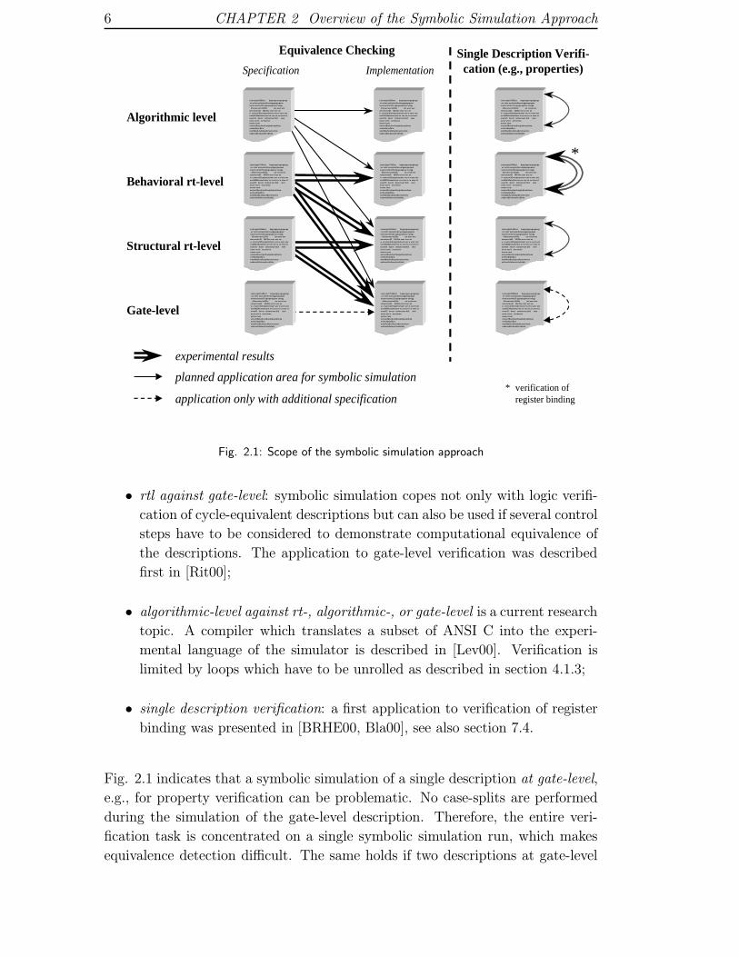
descriptions at different levels of abstraction. Fig. 2.1 summarizes graphically

the scope of the simulator:

• rtl against rtl: the descriptions can have different implementation details

and the number of control steps to compute a result may vary;

– behavioral-rtl against behavioral-rtl: experimental results for the ver-

ification of automatically constructed pipelined processors were pre-

sented first in [HER99]. The results in [RHE99] demonstrate that

our symbolic simulation also copes with distinct orders of memory

operations in the two descriptions to be compared;

– behavioral-rtl against structural-rtl: the structural implementation of

an architecture with microprogram control has been compared to be-

havioral specifications in [REH99]. The implementation details of the

structural description and the fact that a different number of sequen-

tial steps has to be considered makes verification complex. Verifica-

tion results for structural descriptions with different implementation

details of pipelined DLX-processors are reported in [REH99], too;

1An empty loop body is simulated if the number of executions is smaller.


Single Description Verifi-cation (e.g., properties)

Equivalence Checking

Algorithmic level

rwirwejert5345ert keqweqwewqwqewqe wr erter owiweter4erwerqqweqwqweewwerwrertert35 eqwqweqewse rweqq 45wrwrwer\et534r ser were werserwerrwe45 34535w erwr wer wew erwerw3i3rwejertertwer wer w weer werwro34534wiweterwer we rwe rw rw erwe rtwwer35 4wrer tertwerwer fesf eeeewrwr wer\e werwerwe werwe rwer werwerlkwer[werkwejorkwenrlwenwrelwekrjwlkrwweerlkwekrwlerjwekrwerwerewwekrwelrlwlwerwlrwlrlwlr


Behavioral rt-level



Structural rt-level


Gate-level



experimental results

planned application area for symbolic simulation

application only with additional specification

Specification Implementation






*

* verification ofregister binding

Fig. 2.1: Scope of the symbolic simulation approach

• rtl against gate-level: symbolic simulation copes not only with logic verifi-

cation of cycle-equivalent descriptions but can also be used if several control

steps have to be considered to demonstrate computational equivalence of

the descriptions. The application to gate-level verification was described

first in [Rit00];

• algorithmic-level against rt-, algorithmic-, or gate-level is a current research

topic. A compiler which translates a subset of ANSI C into the experi-

mental language of the simulator is described in [Lev00]. Verification is

limited by loops which have to be unrolled as described in section 4.1.3;

• single description verification: a first application to verification of register

binding was presented in [BRHE00, Bla00], see also section 7.4.

Fig. 2.1 indicates that a symbolic simulation of a single description at gate-level,

e.g., for property verification can be problematic. No case-splits are performed

during the simulation of the gate-level description. Therefore, the entire veri-

fication task is concentrated on a single symbolic simulation run, which makes

equivalence detection difficult. The same holds if two descriptions at gate-level

2.3 Introductory Examples 7

are compared, see left-hand side of Fig. 2.1 (dotted arrow).2 Providing a specifi-

cation at a higher abstraction level allows also verifying these gate-level problems.

The simulation of the specification at higher level is used to ”guide” the path

search or symbolic simulation of the gate-level description, see section 4.6. The

verification task is divided since the specification defines the respective path to

be simulated at gate-level.

2.3 Introductory Examples

Two examples are used to introduce the symbolic simulation approach. Note that

these examples do not cover the verification scope as described in the previous

section:

• the application area of the symbolic simulator to verify descriptions at

different levels of abstraction is larger, see above,

• only equivalence checking is considered, and

• a sequential verification over several cycles is necessary for both examples,

but the intermediate results are the same; this is not required for compu-

tational equivalence.

The first example (rt-level⇔rt-level) is used to give a first idea of the basic simu-

lation procedure. The second example introduces verification at gate-level. Sec-

tion 4.5 describes the symbolic simulation of both examples by the implemented

verification tool.

Example 2.1

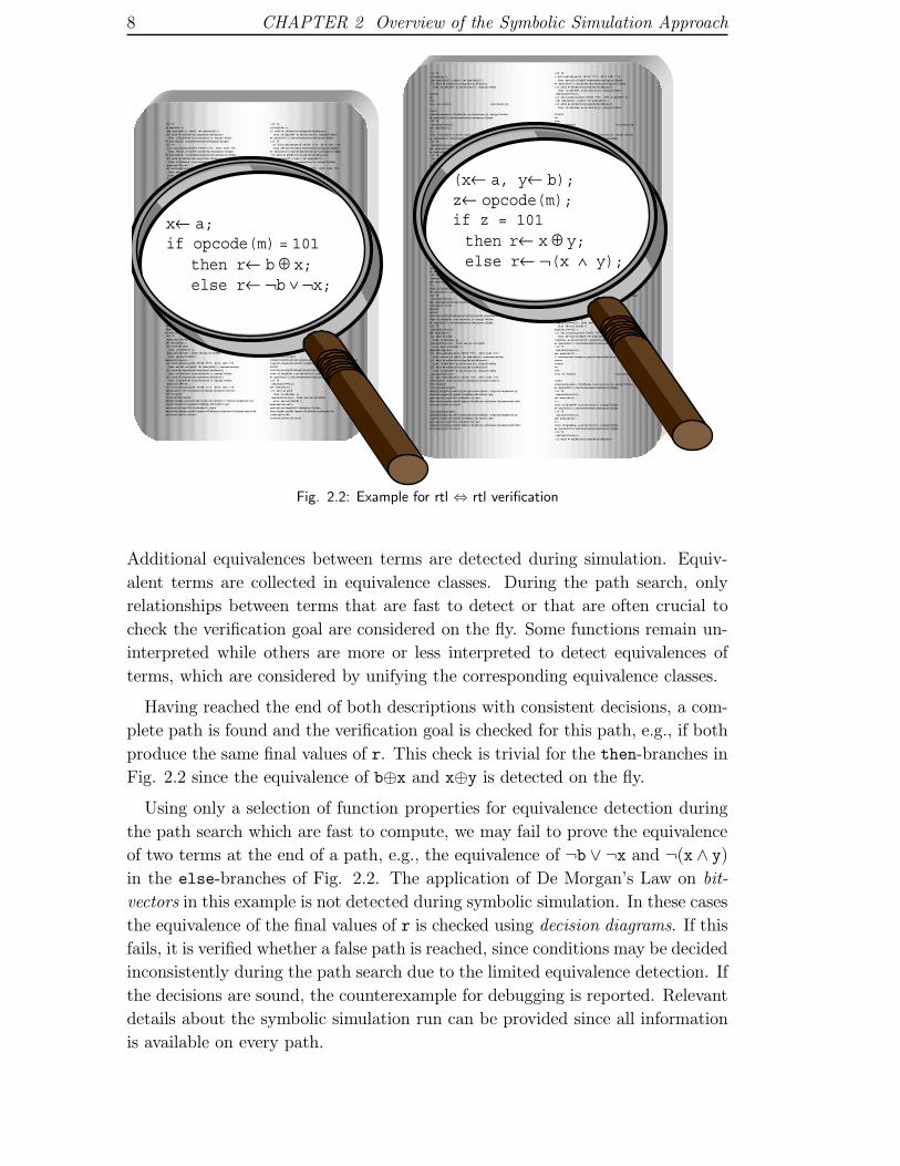
Fig. 2.2 describes two computationally equivalent parts of two descriptions at

rt-level. Equivalence is given with respect to the final value of the register r.

The equivalence checker simulates symbolically all possible paths. False paths

are avoided by making only consistent decisions at branches in the description.

A case-split is performed if a condition is reached which cannot be decided but

depends on the initial register and memory values, e.g., opcode(m)=101 in Ex-

ample 2.1. The example requires the symbolic simulation of two paths since the

other condition z=101 has to be decided consistently. Note that both symbolic

paths represent an important number of ”classical” simulation runs.

Each symbolically executed assignment establishes an equivalence between the

destination variable on the left and the term on the right side of an assignment.

2This verification step can be done efficiently by other techniques, e.g., combinational equiv-

alence checking if the circuit is not retimed.


(if 78

rf[adrB]← b, x← mem[adr2]);twert (← mem[adr2]); (if adrA ≠ adrBertetioerptkerotk8iperot then rf[adrA]← a;erteroterj[o ermjgi7ethbe

erweirwerwereri we ewroiw weioruwerijw

oewri

efwerwerwethen rf[adrA]← a;erteroterj[o ermjgi7ethbe← mem[adr2]);twertwerwerweroewihgoerijhgbe(if 78

mem[adr1]←val);x← mem[adr2]);l);then rf[adrA]← a;erteroterj[o ermjgi7ethbe

← mem[adr2]);twertwerwerweroewihgoerijhgbe(if 78

mem[adr1]←val);x← mem[adr2]);← mem[adr2]);twertwerwerweroewihgoerijhgbe(if 78 (if adr1=adr2etyer54 78768 7776 8676 i68i 778 then z←val+rf[adrR werwerweroewihgoerijhgbe← mem[adr2]);twersfawetwerwerweroewihgoerijhgbe(if adrA ≠ adrBertetioerptkerotk8iperot then rf[adrA]← a;erteroterj[o ermjgi7ethbe mem[adr1]←val);(if adr1=adr2etyer54 78768 7776 8676 i68i 778

then z←val+rf[adrR]7 878 i78 i87 i else z←x+rf[adrR]);7i 7878 78then z←val+rf[adrR]7 878 i78 i87 i else z←x+rf[adrR]);7i 7878 (if adr1=adr2 78

mem[adr1]←vawerwesrwaerwearwerwerwerawerawerwarwearl);

then rf[adrA]← a;erteroterj[o ermjgi7ethbe← mem[adr2]);twertwerwerweroewihgoerijhgbe(if 78 mem[adr1]←val);x← mem[adr2]);l);werwerweoiruwepoir,pweiurcmpouopeiwurwrwerwerweirwerwe

reri we ewroiw weioruwerijw

oewriefwerwerwethen rf[adrA]← a;erteroterj[o ermjgi7ethbe


mem[adr1]←val);x← mem[adr2]);l);

then rf[adrA]← a;erteroterj[o ermjgi7ethbe← mem[adr2]);twertwerwerweroewihgoerijhgbe(if 78 mem[adr1]←val);x← mem[wwerwerwerwaerwdr2]);wrwerwerl);erwrwerwerwerwerwet5erioustgnfodsegkjerogtkjerogtkjerogtkmeorkegmrkhmge

then rf[adrA]← a;erteroterj[o ermjgi7ethbe← mem[adr2]);twertwerwerweroewihgoerijhgbe(if 78 mem[adr1]←val);x← mem[adr2]);(if adrA ≠ adrB then rf[adrA]← a; mem[adr1]←val); then z←val+rf[adrR] else z←x+rf[adrR]);mem[adr1]←val);(if adr1=adr2etyer54 78768 7776 8676 i68i 778

then z←val+rf[adrR (← mem[adr2]);twerweroewihg(if adrA ≠ adrBertetioerptkerotk8iperot then rf[adrA]← a;erteroterj[o ermjgi7ethbe(if adrA ≠ adrBertetioerptkerotk8iperot then rf[adrA]← a;erteroterj[o ermjgi7ethbe mem[adr1]←val);(if adr1=adr2etyer54 78768 7776 8676 i68i 778ewrwerawer ewvtroiejwcro[iwehjnr[occwn3r[oweictweticwopjer

tijeroginhreisgvbsdrpgvjnsdprigjzseriogjerogh;serozighzr;‘ongvosrzegmnseirogregoerijngerzos[goxdrijzdghnb;zdriozdjo‘gergeroigtjer[ognifd;lindzgher[tjisereartoearjiopgb;zjndfl/gmnio;dlzkhrje;oyhinser[ohinmstophtrfshsrtyoeaijyeoritisoert

tijeroginhreisgvbsdrpgvjnsdprigjzseriogjerogh;serozighzr;‘ongvosrzegmnseirogregoerijngerzos[goxdrijzdghnb;zdriozdjo‘ger

geroigtjer[ognifd;lindzgher[tjisereartoearjiopgb;zjndfl/gmnio;dlzkhrje;oyhinser[ohinmstophtrfshsrtyoeaijyeoritisoert

(if 78r adr1=adr2etyer54 78768 7776 8676 i68i 778

then z←val+rf[adrR werwerweroewihgoerijhgbe← mem[adr2]);twersfawetwerwerweroewihgoerijhgbe(if adrA ≠ adrBertetioerptkerotk8iperot then rf[adrA]← a;erteroterj[o ermjgi7ethbe mem[adr1]←val);(if adr1=adr2etyer54 78768 7776 8676 f[adrB]← b, x← mem[adr2]);twert (← mem[adr2]); (if adrA ≠ adrBertetioerptkerotk8iperot then rf[adrA]← a;erteroterj[o ermjgi7ethbe

erweirwerwe

reri we ewroiw weioruwerijw

oewriefwerwerwethen rf[adrA]← a;erteroterj[o ermjgi7ethbe


mem[adr1]←val);x← mem[adr2]);l);

then rf[adrA]← a;erteroterj[o ermjgi7ethbe← mem[adr2]);twertwerwerweroewihgoerijhgbe(if 78 mem[adr1]←val);x← mem[adr2]);

← mem[adr2]);twertwerwerweroewihgoerijhgbe(if 78 (if i68i 778

then z←val+rf[adrR]7 878 i78 i87 i else z←x+rf[adrR]);7i 7878 78then z←val+rf[adrR]7 878 i78 i87 i else z←x+rf[adrR]);7i 7878 (if adr1=adr2adr1=adr2etyer54 78768 7776 8676 i68i 778

then z←val+rf[adrR werwerweroewihgoerijhgbe← mem[adr2]);twersfawetwerwerweroewihgoerijhgbe(if adrA ≠ adrBertetioerptkerotk8iperot then rf[adrA]← a;erteroterj[o ermjgi7ethbe mem[adr1]←val);(if adr1=adr2etyer54 78768 7776 8676 ermjgi7ethbe← mem[adr2]);twertwerwerweroewihgoerijhgbe(if 78 mem[adr1]←val);

x← mem[adr2]);l);

then rf[adrA]← a;erteroterj[o ermjgi7ethbe← mem[adr2]);twertwerwerweroewihgoerijhgbe(if 78

mem[adr1]←val);x← mem[adr2]);l);then rf[adrA]← a;erteroterj[o ermjgi7ethbe


mem[adr1]←val);x← mem[wwerwerwerwaerwdr2]);wrwerwerl);erwr

werwerwerwerwet5erioustgnfodsegkjerogtkjerogtkjerogtkmeorkegmrkhmgethen rf[adrA]← a;erteroterj[o ermjgi7ethbe← mem[adr2]);twertwerwerweroewihgoerijhgbe(if 78

mem[adr1]←val);x← mem[adr2]);(if adrA ≠ adrB then rf[adrA]← a; mem[adr1]←val); then z←val+rf[adrR] else z←x+rf[adrR]);mem[adr1]←val);(if adr1=adr2etyer54 78768 7776 8676 i68i 778 then z←val+rf[adrR (← mem[adr2]);twerweroewihg

[adrA]← a;erteroterj[o ermjgi7ethbe← mem[adr2]);twertwerwerweroewihgoerijhgbe(if 78

mem[adr1]←val);x← mem[adr2]);l);werwerweoiruwepoir,pweiurcmpouopeiwurwrwerwerweirwerwereri we ewroiw weioruwerijw

oewri

efwerwerwethen rf[adrA]← a;erteroterj[o ermjgi7ethbe← mem[adr2]);twertwerwerweroewihgoerijhgbe(if 78 mem[adr1]←val);x← mem[adr2]);l);


mem[adr1]←val);x← mem[adr2]);l);then rf[adrA]← a;erteroterj[o ermjgi7ethbe← mem[adr2]);twertwerwerweroewihgoerijhgbe(if 78 mem[adr1]←val);

(if adrA ≠ adrBertetioerptkerotk8iperot

(if 78

rf[adrB]← b, x← mem[adr2]);twert (← mem[adr2]); (if adrA ≠ adrBertetioerptkerotk8iperot then rf[adrA]← a;erteroterj[o ermjgi7ethbe← mem[adr2]);twertwerwerweroewihgoerijhgbe(if 78 (if adr1=adr2etyer54 78768 7776 8676 i68i 778 then z←val+rf[adrR werwerweroewihgoerijhgbe← mem[adr2]);twersfawetwerwerweroewihgoerijhgbe

(if adrA ≠ adrBertetioerptkerotk8iperot then rf[adrA]← a;erteroterj[o ermjgi7ethbe mem[adr1]←val);(if adr1=adr2etyer54 78768 7776 8676 i68i 778


mem[adr1]←vawerwesrwaerwear

werwerwerawerawerwarwearl);then rf[adrA]← a;erteroterj[o ermjgi7ethbe← mem[adr2]);twertwerwerweroewihgoerijhgbe(if 78

mem[adr1]←val);x← mem[adr2]);l);werwerweoiruwepoir,pweiurcmpouopeiwurwrwerwerweir

werwereri we ewroiw weioruwerijw

oewri



x← mem[adr2]);l);


mem[adr1]←val);x← mem[wwerwerwerwaerwdr2]);wrwerwerl);erwrwerwerwerwerwet5erioustgnfodsegkjerogtkjerogtkjerogtkmeorkegmrkhmge


mem[adr1]←val);x← mem[adr2]);(if adrA ≠ adrB then rf[adrA]← a; mem[adr1]←val); then z←val+rf[adrR]

else z←x+rf[adrR]);mem[adr1]←val);(if adr1=adr2etyer54 78768 7776 8676 i68i 778

then z←val+rf[adrR (← mem[adr2]);twerweroewihg(if adrA ≠ adrBertetioerptkerotk8iperot then rf[adrA]← a;erteroterj[o ermjgi7ethbe(if adrA ≠ adrBertetioerptkerotk8iperot then rf[adrA]← a;erteroterj[o ermjgi7ethbe mem[adr1]←val);(if adr1=adr2etyer54 78768 7776 8676 i68i 778ewrwerawer ewvtroiejwcro[iwehjnr[occwn3r[oweictweticwopjertijeroginhreisgvbsdrpgvjnsdprigjzseriogjerogh;serozighzr;‘ongvosrzegmnseirogregoerijngerzos[goxdrijzdghnb;zdriozdjo‘ger

geroigtjer[ognifd;lindzgher[tjisereartoearjiopgb;zjndfl/gmnio;dlzkhrje;oyhinser[ohinmstophtrfshsrtyoeaijyeoritisoert

(if 78

rf[adrB]← b,if adrA ≠ adrBertetioerptkerotk8iperot then rf[adrA]← a;erteroterj[o ermjgi7ethbe← mem[adr2]);twertwerwerweroewihgoerijhgbe(if 78 (if adr1=adr2etyer54 78768 7776 8676 i68i 778 then z←val+rf[adrR werwerweroewihgoerijhgbe← mem[adr2]);twersfawetwerwerweroewihgoerijhgbe(if adrA ≠ adrBertetioerptkerotk8iperot x← mem[adr2]);twert (← mem[adr2]); (then rf[adrA]← a;erteroterj[o ermjgi7ethbe mem[adr1]←val);(if adr1=adr2etyer54 78768 7776 8676 i68i 778

the adr1]←vawerwesrwaerwearwerwerwerawerawerwarwearl);then rf[adrA]← a;erteroterj[o ermjgi7ethbe← mem[adr2]);twertwerwerweroewihgoerijhgbe(if 78

mem[adr1]←val);x← mem[adr2]);l);werwerweoiruwepoir,pweiurcmpouopeiwurwrwerw


oewri


mem[adr1]←val);x← mem[adr2]);l);then rf[adrA]← a;erteroterj[o ermjgi7ethbe ni87 i else z←x+rf[adrR]);7i 7878 78

then z←val+rf[adrR]7 878 i78 i87 i else z←x+rf[adrR]);7i 7878 (if adr1=adr2

78 mem[← mem[adr2]);twertwerwerweroewihgoerijhgbe(if 78 mem[adr1]←val);

x← mem[adr2]);l);


mem[adr1]←val);x← mem[wwerwerwerwaerwdr2]);wrwerwerl);erwrwerwer(if adr1=adr2etyer54 78768 7776 8676 i68i 778

then z←val+rf[adrR (← mem[adr2]);twerweroewihg(if adrA ≠ adrBertetioerptkerotk8iperot then rf[adrA]← a;erteroterj[o ermjgi7ethbe(if adrA ≠ adrBertetioerptkerotk8iperot then rf[adrA]← a;erteroterj[o ermjgi7ethbe mem[adr1]←val);(if adr1=adr2etyer54 78768 7776 8676 i68i 778ewrwerawer ewvtroiejwcro[iwehjnr[occwn3r[oweictweticwopjertijeroginhreisgvbsdrpgvjnsdprigjzseriogjerogh;serozighzr;‘ongvosrzegmnseirogregoerijngerzos[goxdrijzdghnb;zdriozdjo‘gerwerwerwet5erioustgnfodsegkjerogtkjerogtkjerogtkmeorkegmrkhmge

then rf[adrA]← a;erteroterj[o ermjgi7ethbe← mem[adr2]);twertwerwerweroewihgoerijhgbe(if 78 mem[adr1]←val);x← mem[adr2]);

(if adrA ≠ adrB then rf[adrA]← a; mem[adr1]←val); then z←val+rf[adrR] else z←x+rf[adrR]);mem[adr1]←val);geroigtjer[ognifd;lindzgher[tjiserearjiopgb;zjndfl/gmnio;dlzkhrje;oyhinser[ohinmstophtrfshsrtyoeaijyeoritisoert

x← a;if opcode(m) = 101

then r← b ⊕ x;else r← ¬b ∨ ¬x;

(x← a, y← b);z← opcode(m);if z = 101then r← x ⊕ y;else r← ¬(x ∧ y);

Fig. 2.2: Example for rtl ⇔ rtl verification

Additional equivalences between terms are detected during simulation. Equiv-

alent terms are collected in equivalence classes. During the path search, only

relationships between terms that are fast to detect or that are often crucial to

check the verification goal are considered on the fly. Some functions remain un-

interpreted while others are more or less interpreted to detect equivalences of

terms, which are considered by unifying the corresponding equivalence classes.

Having reached the end of both descriptions with consistent decisions, a com-

plete path is found and the verification goal is checked for this path, e.g., if both

produce the same final values of r. This check is trivial for the then-branches in

Fig. 2.2 since the equivalence of b⊕x and x⊕y is detected on the fly.

Using only a selection of function properties for equivalence detection during

the path search which are fast to compute, we may fail to prove the equivalence

of two terms at the end of a path, e.g., the equivalence of ¬b ∨ ¬x and ¬(x ∧ y)

in the else-branches of Fig. 2.2. The application of De Morgan’s Law on bit-

vectors in this example is not detected during symbolic simulation. In these cases

the equivalence of the final values of r is checked using decision diagrams. If this

fails, it is verified whether a false path is reached, since conditions may be decided

inconsistently during the path search due to the limited equivalence detection. If

the decisions are sound, the counterexample for debugging is reported. Relevant

details about the symbolic simulation run can be provided since all information

is available on every path.

2.3 Introductory Examples 9

Example 2.2

Fig. 2.3 compares a specification at rt-level and an implementation at gate-level.

⊕

&

⊕

&

⊕

&⊕

&&

⊕

&&

⊕

&&

⊕

&&

&

⊕

&&

⊕

&&

⊕

&&

⊕

&& ⊕

⊕

&⊕

&&

⊕

&&

&

⊕

&&

⊕

&&

⊕

&&

⊕

&&

⊕

&&

⊕

&&

⊕

&&

⊕

&&

⊕

⊕

&

⊕

&&

&

⊕

&&

⊕&

⊕

⊕

&

⊕

&&

&

⊕

&&

⊕

&&

⊕

⊕

&

⊕

&&

&

⊕

&&

⊕

&&

⊕

&&

⊕

&&

⊕

&&

⊕

&&

⊕

&&

⊕

&&

⊕

⊕

&

⊕

&&

&

⊕

&&

⊕

&&

⊕

⊕

&

⊕

&&

&

⊕

&&

⊕

&

⊕

&&

⊕

&

&

⊕

&&

⊕

&

⊕

&&

⊕

&

&

⊕

&&

⊕

&

⊕

&&

⊕

&

&

⊕

&&

⊕

&

&&

⊕

&&

⊕

&&

⊕

&&

⊕

&&

⊕

&&

⊕

&&

⊕

&&

⊕ &

⊕

&&

⊕

&&

⊕

&&

⊕

&&

⊕

&&

⊕

&&

⊕

&&

⊕

&&

⊕

&&

⊕

&&

⊕

&&

⊕

&&

⊕

&&

⊕

&&

⊕

⊕

&

⊕

&&

&

⊕

&&

⊕

&&

⊕

&&

⊕

&&

⊕

&&

⊕

&&

&&

⊕

&&

&

⊕

&&

⊕

&⊕

&&

⊕

&&

⊕

&&

⊕

&&

⊕

&

⊕

&

⊕

&⊕

&&

⊕

&&

⊕

&&

⊕

&&

&

⊕

&&

⊕

&&

⊕

&&

⊕

&&

⊕

⊕

&

⊕

&&

&

⊕

&&

⊕&

⊕

&&

⊕

&&

⊕

&&

⊕

&&

⊕

&&

⊕

⊕

&

⊕

&&

&

⊕

&&

⊕

&&

⊕

⊕

&

⊕

&&

&

⊕

&&

⊕

&&

&

⊕

&

⊕

&

&⊕

&&

⊕

&&

⊕

&&

⊕

&&

⊕

&&

⊕

&&

⊕

⊕

&

⊕

&&

&

⊕

&&

⊕

&&

⊕

⊕

&

⊕

&&

&

⊕

&&

⊕

&

⊕

&&

⊕

&

&

⊕

&&

(if 78

rf[adrB]← b, x← mem[adr2]);twert (← mem[adr2]); (if adrA ≠ adrBertetioerptkerotk8iperot then rf[adrA]← a;erteroterj[o ermjgi7ethbe← mem[adr2]);twertwerwerweroewihgoerijhgbe(if 78 (if adr1=adr2etyer54 78768 7776 8676 i68i 778 then z←val+rf[adrR werwerweroewihgoerijhgbe← mem[adr2]);twersfawetwerwerweroewihgoerijhgbe

(if adrA ≠ adrBertetioerptkerotk8iperot then rf[adrA]← a;erteroterj[o ermjgi7ethbe mem[adr1]←val);(if adr1=adr2etyer54 78768 7776 8676 i68i 778


mem[adr1]←vawerwesrwaerwear

werwerwerawerawerwarwearl);then rf[adrA]← a;erteroterj[o ermjgi7ethbe← mem[adr2]);twertwerwerweroewihgoerijhgbe(if 78

mem[adr1]←val);x← mem[adr2]);l);werwerweoiruwepoir,pweiurcmpouopeiwurwrwerwerweir

werwereri we ewroiw

oewri

efwerwerwethen rf[adrA]← a;← mem[adr2]);twertwerwerweroewihgoerijhgbe(if 78


x← mem[adr2]);l);


mem[adr1]←val);x← mem[wwerwerwerwaerwdr2]);wrwerwerl);erwrwerwerwerwerwet5erioustgnfodsegkjeromge


mem[adr1]←val);x← mem[adr2]);(if adrA ≠ adrB then rf[adrA]← a; mem[adr1]←val); then z←val+rf[adrR]

else z←x+rf[adrR]);mem[adr1]←val);(if adr1=adr2etyer54 78768 7776 8676 i68i 778

then z←val+rf[adrR (← mem[adr2]);twerweroewihg(if adrA ≠ adrBertetioerptkerotk8iperot then rf[adrA]← a;erteroterj[o ermjgi7ethbe(if adrA ≠ adrBertetioerptkerotk8iperot then rf[adrA]← a;erteroterj[o ermjgi7ethbe mem[adr1]←val);(if adr1=adr2etyer54 78768 7776 8676 i68i 778ewrwerawer ewvtroiejwcro[iwehjnr[occwn3r[oweictweticwopjertijeroginhreisgvberogh;serozighzr;‘ongvosrzegmnseirogregoerijngerzos[goxdrijzdghnb;zdriozdjo‘ger

geroigtjer[ognifd;lindzgher[tjisereartoearjiopgb;zjndfl/gmnio;dlzkhrje;

(if 78

rf[adrB]← b,if adrA ≠ adrBertetioerptkerotk8iperot then rf[adrA]← a;← mem[adr2]);twertwerwerweroewihgoerijhgbe(if 78 (if adr1=7776 8676 i68i 778← mem[adr2]);twersfaeroewihgoerijhgbe(if adrA ≠ adrBe8iperot x← mem[adr2]);twert (← mem[adr2]); (then rf[adrA]← o ermjgi7ethbe mem[adr1]←val);(if adr1=adr2etyer54 78768 7776 8676 i6

the adr1]←vawerwesrwaer

wearwerwerwerawerawerwarwearl);then rf[adrA]← a;erteroterj[o ermjgi7ethbe← mem[adr2]);twertwerwerweroewihgoerijhgbe(if 78

mem[adr1]←val);x← mem[adr2]);l);werwerweoiruwepoir,pweiurcmpouopeiwurwrwerw


oewri

efwerwerwethen rf[adrA]← a;(if 78

mem[adr1]←val);x← mem[adr2]);l);then rf[adrA]← a; ni87 i else z←x+rf[adrR]);7i 7878 78then z←val+rf[adrR]7 878 i78 i87 i

else z←x+rf[adrR]);7i 7878 (if adr1=adr2 78 mem[

← mem[adr2]);twertwerwerweroewihgoerijhgbe(if 78 mem[adr1]←val);x← mem[adr2]);l);


mem[adr1]←val);x← mem[wwerwerwerwaerwdr2]);wrwerwerl);erwrwerwer(if adr1=adr2etyer54 78768 7776 8676 i68i 778 then z←val+rf[adrR (← mem[adr2]);twerweroewihg

(if adrA ≠ adrBertetioerptkerotk8iperot then rf[adrA]← a;erteroterj[o ermjgi7ethbe(if adrA ≠ adrBertetioerptkerotk8iperot then rf[adrA]← a;erteroterj[o ermjgi7ethbe mem[adr1]←val);(if adr1=adr2etyer54 78768 7776 8676 i68i 778ewrwerawer ewvtroiejwcro[iwehjnr[occwn3r[oweictweticwopjertijeroginhreisgvb

regoerijngerzos[goxdrijzdghnb;zdriozdjo‘gerwerwerwet5erioustgnfodsegkjgtkmeorkegmrkhmge

then rf[adrA]← a;← mem[adr2]);twertwerwerweroewihgoerijhgbe(if 78 mem[adr1]←val);x← mem[adr2]);(if adrA ≠ adrB then rf[adrA]← a; mem[adr1]←val); then z←val+rf[adrR] else z←x+rf[adrR]);mem[adr1]←val);geroigtjer[ognifd;lindzgher[tjiser

earjiopgb;zjndfl/gmnio;dlzkhrje;oyhinser[ohinmstophtrfshsrtyoeaijyeoritisoert

r← r+1;if m = 0

then r← r+1;else r← 000;

r[2]

clk

&

r[1]&

r[0]&

r

⊕

⊕

&

&

clk

ctrlm

Fig. 2.3: Example for rtl ⇔ gate-level verification

They are computational equivalent with respect to the register r if ctrl is

initialized with 0 and if the execution takes two cycles. The implementation

at gate-level includes the signal assignments to the three bits of the register r

and to the control flag ctrl. Two cycles of symbolic simulation are required

to demonstrate equivalence. In the first cycle, r+1 is calculated and ctrl is set

true. The if-then-else-clause evaluating the flag m is considered in the next cycle.

Symbolic simulation has to demonstrate that the final values of r are the same.

Two cycles have to be simulated symbolically in the example of Fig. 2.3. There-

fore, the gate-level description representing only one cycle is put together for

two times before simulating, i.e., the description is replicated accordingly to the

number of cycles required. The values of the registers of the previous simulation

cycle are the input values of the next cycle, see Fig. 2.4.


cycle 1 cycle 2

r[2]

clk

&

r[1]&

r[0]&

r

⊕

⊕

&

&

clk

ctrlm

r[2]

r[1]

r[0]

ctrl

r[2]

clk

&

r[1]&

r[0]&

r

⊕

⊕

&

&

clk

ctrlm

initialsymbolicvalues

finalsymbolicvalues

Fig. 2.4: Duplicating a gate-level description

2.4 Distinguishing Different Register Values

The values of each register being assigned in several cycles are distinguished by

indexing. We do not substitute the register in the following by the symbolic

term assigned to it to avoid term-size explosion. An indexed register name is

called a RegVal. A new RegVal with an incremented index is introduced after

each assignment to a register. An additional upper index s or i distinguishes the

RegVals of the specification and of the implementation. For example, ar←a+b;

is replaced by ars2 ←as1+bs1; in the specification if all registers have already

been assigned once. Only the initial RegValsinitial as anchors are identical in

the specification and in the implementation, since the equivalence of the two

descriptions is tested with respect to arbitrary but identical initial register values.

RegVals are also used to distinguish the different states of a memory. A new

RegVal with an incremented index is introduced after each store-operation to a

memory. For example, the third store-operation to a memory mem[adr]←val;

becomes mems3 ← store(mems2, adrs1, val

s1). The RegVals mems2 and mems3 represent

the memory state before and after the store-operation.

Definition 2.1 (RegVal)

A RegVal represents

• the initial symbolic value of a register,

• the symbolic value of a register after an assignment until the next assign-

ment to the same register,

2.5 Internal Representation for Symbolic Simulation 11

• the initial symbolic state of a memory, or

• the symbolic state of a memory after a store-operation until the next

store-operation to the same memory.

2.5 Internal Representation for

Symbolic Simulation

The descriptions simulated symbolically consist of:

• lists of assignments to RegVals; the expressions assigned are other RegVals,

constants, or terms, i.e., functions of RegVals; note that memory access is

modeled by read- and store-operations;

• if-then-else-clauses; both branches can contain a list of assignments to Reg-

Vals and/or several if-then-else-clauses. Symbolic simulation forks at each

if-then-else, which requires a case-split on the corresponding condition.

Parallel assignments are considered implicitly by the indexes of the RegVals.

Other control structures, e.g., case-clauses or multiplexers are compiled into if-

then-else-clauses.3

In general, at least one of the descriptions to be compared contains if-then-else-

clauses. Gate-level descriptions consist only of assignments to RegVals. Interme-

diate signals are either substituted by the corresponding expression until primary

inputs or the output of flip-flops is reached; or they are considered for technical

reasons as ”artificial” RegVals.4 Primary inputs are modeled by RegVals, too.

Compilation of descriptions at structural or behavioral rt-level is straightforward.

Section 4.1 describes the preparation of the data structure.

2.6 Detecting Equivalences of Symbolic Terms

Symbolic simulation argues about symbolic terms which represent a set of differ-

ent values. The actual value selected from this set depends on the initialization of

the registers and memories. Deciding whether two terms are equivalent is trivial

in numerical simulation, but not obvious if symbolic terms are used. Intuitively,

two terms or RegVals are equivalent if an exhaustive numerical simulation of each

possible initialization produce in all cases the same value for both terms.

3Note that this is only an implementation choice.4The corresponding expression is assigned to this ”artificial” RegVal, see ”simulation-

cutpoints” in appendix 9.3.


Equivalence of two terms can depend on the actual path followed during sym-

bolic simulation.

Definition 2.2 (Path)

Let C be a set of conditions. A path consists of associating the value true or false

to each condition in C.

The decisions of a path guarantee that specification and implementation can be

simulated until both ends are reached without requiring additional case-splits

at if-then-else-clauses; i.e., no condition occurs which depends on the initial

RegVals on the assumptions concerning C. A partial path permits simulating

without additional case-splits until the two ends of the partial path in both the

specification and the implementation are reached. Note that a branch denotes

only one of the two possibilities of a single if-then-else-clause, i.e., the then- or

the else-branch.5 A path comprises mostly decisions about conditions of more

than one if-then-else-clause.

The following definition of equivalence considers complete and partial paths

by referring to acceptable initializations. The set of combinations of acceptable

initial RegVals is constrained:

• by the domain(RegV alinitial,k) of the RegVal; the index k distinguishes

RegVals of different registers; the type of a register can be integer or bit-

vector;6 the bit-vector length of the register constrains the domain in the

second case; additional restrictions can be defined by the user, i.e., to

exclude impossible initializations;

• by case-splits, leading to one of the decisions about a condition; C =

{C0, · · · , Cn} subsumes all conditions requiring a case-split.

Definition 2.3 (Evaluation of a term or RegVal)

eval(t) =

t is a constant : t

t is a RegV alinitial,k : init(RegV alinitial,k)

t is a RegV alj �=initial,k : eval(t′)

t′ : right-hand side term of

assignment to RegV alj,kt = F (a0, · · · , al) : F (eval(a0), · · · , eval(al))

Definition of eval(t) supposes that all registers and functions are typed with

domains on which equality = is available.

eval(t) returns a constant for an acceptable initialization.

5elsif-clauses can be considered as sequences of if-then-else-clauses.6Note that the decision diagram based tests described in chapter 6 are not applicable for

integers if no information about the range is given.

2.6 Detecting Equivalences of Symbolic Terms 13

Definition 2.4 (Acceptable initialization)

Acceptable initializations of the registers in the descriptions are:

acceptable(initRegV als) ⇔(∀RegV alinitial,k : init(RegV alinitial,k) is a constant ∧

init(RegV alinitial,k) ∈ domain(RegV alinitial,k))∧

∀Ci ∈ C : eval(Ci) is a constant ∧{

Ci decided true : eval(Ci) = 1

Ci decided false : eval(Ci) = 0

The evaluation of the conditions in C guarantees that a given initialization does

not violate one of the decisions. The constants 1 and 0 represent true and

false. Definition of an acceptable initialization supposes that any term used as

condition in an if-then-else-clause evaluates to one of these values. An extension

of the definition for RegVals of memories is given in section 4.1.5.

Definition 2.5 (Valid path)

A valid path - in contrast to a false path - implies that at least one acceptable

initialization exists according to Definition 2.4.

Definition 2.6 (Equivalence of terms)

Two terms or RegVals t1 and t2 are term-equivalent ≡C if under the decisions

taken previously on the path concerning the conditions C = {C0, · · · , Cn} their

values are identical for any acceptable initialization of the RegVals:

t1 ≡C t2 ⇔ ∀initRegV als : acceptable(initRegV als) ⇒ eval(t1) = eval(t2)

Equivalent terms are detected along valid paths, and collected in equivalence

classes (EqvClasses). We write term1∼=C term2 if two terms are in the same

equivalence class established during simulation. If term1∼=C term2 then term1 ≡C

term2. ≡C denotes that the two terms are equivalent according to Definition 2.6

while ∼=C means that the two terms have been identified during symbolic simula-

tion to be ≡C. Equivalence detection on the fly is incomplete as discussed below

to permit a fast symbolic simulation. Therefore, the relationship term1 ≡C term2

might be not revealed, i.e., the terms are still in different EqvClasses. The ex-

pression ”equivalent” is used in the following as synonym for term1∼=C term2.

Initially, each RegVal and each term gets its own equivalence class. Equiva-

lence classes are unified in the following cases:

• two terms are identified to be equivalent by reasoning; the equivalence

detection techniques used are presented in chapter 5 and 6;

• a condition is decided; if this condition is

– a test for equality a = b, then the equivalence classes of both sides are

unified only if the condition is asserted,


– otherwise (e.g., a < b or a status-flag) the equivalence class of the

condition is unified with the equivalence class of the constant 1 or 0

if the condition is asserted or denied;

• after every assignment. Practically, this union-operation is significantly

simpler because the equivalence class of the RegVal on the left-hand side

of the assignment was not modified previously.

Equivalence classes permit to keep also track about inequivalences of terms:

Definition 2.7 (Inequivalence of terms)

Two terms or RegVals t1 and t2 are inequivalent �≡C if under the decisions taken

previously on the path concerning the conditions C = {C0, · · · , Cn} their values

are never identical for any acceptable initialization of the RegVals:

t1 �≡Ct2 ⇔ ∀initRegV als : acceptable(initRegV als) ⇒ eval(t1) �= eval(t2)

Intuitively, two terms are inequivalent if an exhaustive numerical simulation of all

possible initial register values and memory states produces in all cases different

values for the two terms. We write term1 �∼=C term2 or use the expression ”in-

equivalent” if two terms are identified to be �≡C during simulation. Equivalence

classes containing �∼=C terms are inequivalent, too. This is the case

• if different constants are members of the EqvClasses;

• if a condition with a test for equality (e.g., a = b) is decided to be false;

• if terms of the EqvClasses are identified to be inequivalent by reasoning.

Identifying inequivalences during symbolic simulation requires mostly no special-

ized techniques or is done using decision diagrams. The reason is that they are

caused in most of the cases either by the fact that two terms are equivalent to

different constants or by case-splits. On the other hand, detecting equivalences

between symbolic terms is the most important task during symbolic simulation:

• equivalence is the strongest relationship which the two sets of possible

values of two symbolic terms can have: the value for both symbolic terms

is the same for any acceptable initialization of the registers and memories;

• conditions have to be decided consistently during symbolic simulation; con-

ditions are often checks for equality, e.g., a="0001" which can be decided

without case-split if the two terms are previously detected to be equivalent.

All other conditions can also be considered as a check for equality to the

constants 1 or 0, which represent the values true and false.

Example 2.3

The conditions a<5, a[14], or odd(a) are decided without case-split if the

corresponding terms are equivalent to the constants 1 or 0;

2.6 Detecting Equivalences of Symbolic Terms 15

• knowledge about equivalence or inequivalence of two terms is the key in-

formation in most of the cases to decide the relationship of other terms;

Example 2.4

– (not(x) and y) is equivalent to 0 if x is equivalent to y;

– a+b and c+d are equivalent if the arguments are pairwise equivalent;

– two read-operations from a memory result in the same value if the

addresses are equivalent and no intervening store-operation exists;

– if a two-bit vector is inequivalent to the constants 00, 01, and 10, then

it is equivalent to the constant 11.

Chapter 5 discusses how knowledge about equivalences or inequivalences

of the arguments can be used efficiently during symbolic simulation to

discover relationships between terms by reasoning;

• verification goals other than equivalence checking, i.e., property verification

can be reduced to a check for equivalence of terms, too, see section 2.7.

The techniques described in chapter 5 search equivalent terms on the fly de-

pending on the function of this term. Ideally, all ≡C terms and RegVals are in

the same equivalence class, but it is too time consuming to search for all possi-

ble equivalences on the fly. In order to speed up the path search, the following

simplifications are made with respect to a complete equivalence detection:

• only fast to check or “crucial” properties of interpreted functions are con-

sidered;

• only the information of the equivalence classes of the direct arguments is

used in most of the cases to reveal equivalences between terms; i.e., the

equivalence of terms can be decided by simply testing if the arguments

are ∼=C or �∼=C. Expanding the arguments, i.e., tracing the corresponding

expression trees of the arguments is avoided to permit a fast simulation;

• invoking the equivalence detection techniques is restricted as described in

section 4.2.

The incomplete equivalence detection on the fly permits a fast symbolic simula-

tion but may fail to find the equivalence of two terms. Therefore, more accurate

tests called dd-checks based on decision diagrams [Bry86] are used at the end

of a path if the verification goal is not demonstrated. These more powerful, but

also less time-efficient equivalence detection techniques using vectors of OBDDs

are described in chapter 6.

Two terms are frequently equivalent or inequivalent only under the assump-

tions of previous case-splits constraining the set of possible initial RegVals, i.e.,

the relationship is path-dependant.


Example 2.5

A case-split is necessary in the specification of Fig. 2.5 since the value of a=b

Specification

if (a=b) then · · ·else · · ·

xs1 ← a+a;

ys1 ← a vand c;

Implementation

xi1 ← a+b;

yi1 ← b vand c;

Fig. 2.5: Path-dependant equivalence/inequivalence

depends on the initial RegVals. The terms xs1 and xi1 as well as ys1 and yi1 are

equivalent in the case where a=b is asserted. The operator ’vand’ performs the

bit-wise conjunction of the bit-vectors a and c. In the other case xs1 and xi1are inequivalent since the additions result in different values no matter what

the initialization under the assumption a�∼=Cb. The terms ys1 and yi1 are neither

equivalent nor inequivalent since c might be initialized with zero. Therefore, ys1and yi1 may or may not return the same values.

Example 2.5 describes the three basic cases (ternary logic) which can be distin-

guished by using the information of the EqvClasses:

1. two terms are in the same EqvClass; the terms are ∼=C;

2. two terms are in inequivalent EqvClasses; the terms are �∼=C;

3. otherwise they either produce different values for some acceptable initializa-

tion of the RegVals, or equivalence/inequivalence has not yet been detected.

2.7 Rewriting Verification Goals

Checking computational equivalence in a given path consists simply of comparing

the EqvClasses of the respective RegVal-pairs.

Definition 2.8 (Computational equivalence)

Two descriptions are computationally equivalent if both produce the same final

values on the same initial values relative to a set of relevant variables. Let Cbe as in Definition 2.6. For each path characterized by a number of case-splits

leading to the decisions about the conditions in C, the following relation must

hold

∀paths, RegV alsk ∈ RegV alsrelevant : RegV alsfinal,k ≡C RegV alifinal,k

RegVals/ifinal are the corresponding RegVals in the specification and in the imple-

mentation with the highest index in the respective path.7

7The number of assignments to a register can vary depending on the path. Therefore, the

highest index might differ.

2.7 Rewriting Verification Goals 17

Note that not all final RegVals have to be equivalent for computational equiva-

lence, i.e., there might be

• a subset of register/memories appearing only in the implementation, which

can have arbitrary final values, e.g., additional pipeline-registers, and

• a subset of register/memories appearing in the specification which are not

relevant for the equivalence check, e.g., the value of an instruction register.

The description of the symbolic simulation approach in the rest of this work refers

to computational equivalence as verification goal. However, many other verifica-

tion goals can be easily reduced to a check for computational equivalence or the

simulation tool can easily be extended. For example, verifying if two descrip-

tions are trace-equivalent [EHR99], i.e., if all runs coincide step-by-step, requires

comparing not only the final RegVals but all pairs of intermediate RegVals. Note

that one condition for trace-equivalence is that the number of sequential steps in

the two descriptions has to be the same on all paths.

Property verification can often be reduced to a check for computational equiv-

alence by introducing ”fictive” registers which are used as control flags. Those

flags are set on a path if the property is violated. If the annotated description

is computationally equivalent to a ”dummy”-specification which clears only the

corresponding flag then the property is satisfied.

Example 2.6

The register binding verification described in section 7.4 requires checking if there

is no path where a flag check is set to 1 due to an incorrect register binding.

The specification consists of an assignment checks1 ←0, see Fig. 2.6. The same

assignment is added in front of the implementation. The constant 1 is assigned

to check in the following, if a conflict of the register binding is discovered. The

disjunction prevents resetting check in the following. The flag is never set, i.e.,

the register binding is correct iff the descriptions are computationally equivalent

with respect to check.

Specification

checks1 ← 0;

Implementation

checki1 ← 0;�

�

�

�

· · ·checki2 ←checki1 or binding incorrect?

· · ·checki3 ←checki2 or binding incorrect?

· · ·

description

with

annotations

Register binding is verified by checking

computational equivalence with respect to check

Fig. 2.6: Adding control flags for property verification


The verification of arbitrary properties is straightforward corresponding to Fig.

2.6. Usually, the condition binding incorrect? in Fig. 2.6 has to be replaced by

the property to check.

Example 2.7

The following annotations are required to check if

• bit 15 of a register reg is always cleared: checkin ←checkin−1 or regix[15];

• two arbitrary RegVals r1ix and r2iy are equivalent:

checkin ←checkin−1 or not(r1ix ≡r2iy);

• a register does not exceed the value 15: checkin ←checkin−1 or (rix > 15).

Again, the symbolic simulator can provide meaningful information about the

counterexample if the property is not satisfied. Note that inserting the annota-

tions can be supported by the generation of the internal data structure described

in section 4.1, 9.1, and 9.3. For example, the annotation checkin ←checkin−1 or

regix[15] is required only once in a gate-level description even if it has to be

checked in each cycle. Furthermore, the symbolic simulator can be extended to

verify frequently checked properties without additional annotations. Extensions

are facilitated by the fact that the information about each simulation step is

available at the end of a path. Therefore, verification goals concerning inter-

mediate RegVals or terms need not be checked during the path search since the

information does not get lost, e.g., by rewriting terms.

The verification of reactive systems has to consider inputs of a circuit. The

successive values of the inputs are RegVals, too. If the input pattern is known

then the corresponding constants have to be assigned prior to each cycle to the

RegVal of the input. Additional initial RegVals are introduced if the input value

is unknown, i.e., a symbolic input value is used. A new initial RegVal is used for

each input and each cycle. Note that those initial RegVals are identical in the

specification and in the implementation. Intuitively, an input is modeled as a

buffer which provides in each cycle the corresponding constant or a new symbolic

value.

Example 2.8

Assume a gate-level description with an input inport. The implementation at

gate-level has to be simulated for three cycles to check equivalence to a speci-

fication (not shown in Fig. 2.7). The input is reset to ”000” in the first cycle.

The value of the input is arbitrary in the next two cycles. Fig. 2.7 shows the

implementation to be simulated. Two initial RegVals in2 and in3 are assigned to

inport before cycle two and three. The corresponding input values are used in

the gate-level description since the occurrences of inport are accordingly indexed

after each assignment.

2.8 Basic Algorithm of Symbolic Simulation 19

inporti1 ← "000";�� gate-level description using inport

inporti2 ← in2;�� gate-level description using inport

inporti3 ← in3;�� gate-level description using inport

Fig. 2.7: Considering inputs during symbolic simulation

In the rest of this work, we assume, to facilitate the presentation, that the

verification goal to be checked by the symbolic simulator is the computational

equivalence of two descriptions.

2.8 Basic Algorithm of Symbolic Simulation

A brief overview of the basic simulation algorithm is given in the following. The

implemented algorithm is presented more detailed in section 4.6.

The symbolic simulator is designed to compare two acyclic sequences. Fre-

quently, the descriptions cannot be directly compared to demonstrate the veri-

fication goal as in the example of Fig. 2.2. Extracting the two sequences which

demonstrate the verification goal is often simple. For example, two cycles have

to be simulated symbolically to demonstrate the equivalence of the descriptions

in the example of Fig. 2.3.

Algorithm 2.1 gives a simplified overview of the symbolic simulation algorithm

which has been implemented iteratively for optimization, see section 4.6. The

specification and the implementation are simulated in parallel. A case-split is

performed when simulation reaches a condition C that cannot be decided in gen-

eral but depends on the initial register values (lines 2 and 3). The information of

the EqvClasses is used to decide conditions at branches consistently, i.e., to avoid

unnecessary case-splits which lead to false paths. Note that equivalence check is

called recursively in line 3 with only those parts of spec’ and impl’ which are not

simulated yet.

A complete path is found when the end of both descriptions is reached. The

computational equivalence of the descriptions in this path is tested by checking

whether the relevant final RegVals are in the same EqvClass (line 4). This test

may fail since the equivalence detection during the path search is not complete

to permit a fast symbolic simulation. Therefore, the dd-checks based on decision

diagrams are used at the end of a path (line 5). They have to reveal whether

• computational equivalence is given in this path but was not detected (line

6, upper condition),

• a condition has been decided inconsistently due to the incomplete equiv-


alence detection on the fly (line 6, lower condition), i.e., a false path is

detected, or

• a valid counterexample is found (line 7).

All relevant information of the path can be summarized in the last case to facil-

itate debugging. Our automatic verification process does not require insight of

the designer into the verification process.

Algorithm 2.1 Simplified algorithm of the symbolic simulation

equivalence check(spec,impl)

1.

{Simulate spec and impl in parallel and

perform intermediate dd-checks if necessary

}until

(a) a condition C is reached that cannot be decided in general

but depends on the initial register and memory values, or

(b) the end of both descriptions is reached.

2. if a condition C blocks then

3. RETURN(equivalence check (spec′, impl′) |C=FALSE) ∧(equivalence check (spec′, impl′) |C=TRUE)

4. elsif final values of registers are equivalent then RETURN(TRUE)

5. else perform dd-checks;

6. if(final values of registers are equivalent) ∨(a condition has been decided inconsistently)

then RETURN(TRUE)

7. else RETURN(FALSE)

Algorithm 2.1 is slightly modified if one of the descriptions is at gate-level

rather than if both descriptions are at algorithmic-level or rt-level. Intermediate

dd-checks are sometimes useful (line 1) in this case. Furthermore, the descrip-

tions are not simulated in parallel. A complete path is searched instead in the

specification before simulating the implementation at gate-level, see section 4.6.

Chapter 3

Related Work

Section 3.1 gives a brief review of symbolic simulation approaches referring also

to the following sections. A recent symbolic simulation technique called symbolic

trajectory evaluation (STE) is presented separately in section 3.2.

Sections 3.3 to 3.5 compare further formal techniques for sequential verification

to our approach. Techniques based on validity checking, which are related to the

early symbolic simulation approaches, are described in section 3.3. Section 3.4

discusses the use of theorem provers in our application area. Techniques relying

on state space exploration are described in section 3.5.

A selection of semi-formal approaches, which use formal verification tech-

niques, but do not focus on a complete verification, is presented in section 3.6.

Consideration of memories in design verification is discussed separately in section

3.7 since it represents an important part of our symbolic simulator. Finally, sec-

tion 3.8 summarizes the contributions of our work with respect to the approaches

presented in the preceding sections. Techniques performing logic verification or

combinational equivalence checking are not considered in the following since the

purpose of our approach is sequential verification.

3.1 Review of Symbolic Simulation Approaches

Techniques using the principles of symbolic simulation have been used for many

years. ”Symbolic execution” as a technique for software verification was exam-

ined already in the 1970s [Kin75, Kin76, HK76, DK78]. Programs were executed

using symbolic values for variables to demonstrate that they satisfy their speci-

fications.

In the late 1970s ([Dar79] and [CJB79]), researchers at IBM applied the ideas

of symbolic execution to hardware verification. [CJB79] introduced, according

to [Bry90a], the term ”symbolic simulation”.1 [CJB79] checked the equivalence

of specifications and microcoded implementations, i.e., microprograms by exe-

cuting both of them symbolically from corresponding states. Equivalence had to

1Darringer, working also at IBM, still used the term ”symbolic execution” in [Dar79].

21

22 CHAPTER 3 Related Work

be demonstrated for all cases until the next defined point of correspondence was

reached by using simplifiers or/and theorem provers.2 Furthermore, [Dar79] de-

scribes an application to gate-level verification, e.g., comparing a two-bit counter

to a corresponding gate-level description.

These techniques were continued by [Cor81]3 but they turned out to be not

powerful enough at this time to reason about overall circuit behavior [Bry90a].

At each case-split, requiring a decision about a symbolic condition c, the path

conditions of both branches were conjuncted with c and c, respectively [Dar79].

The resulting expressions became too complex to be used efficiently [Bry90a]

and the automatic symbolic manipulation techniques were not powerful enough

[HS97]. Note that demonstrating equivalence of expressions had to be done using

theorem proving techniques (requiring possibly user-interaction) if the previous

simplifications were not sufficient.4

The following symbolic simulation approaches avoided building symbolic ex-

pressions, and used representations closely related to the underlying symbolic

domain. For example, three possible values of a signal {0, 1, X} can be encoded

by two Boolean variables. The advantage of this representation compared to the

previous approaches is that evaluation of functions, i.e., symbolic manipulation

is better supported during simulation, especially by encoding and manipulating

the symbolic signal values by OBDDs [Bry86].5 These techniques were applied

to switch-level verification [Bry85, BBB+87, Bry90b, BF89, JG92].6 STE (Sym-

bolic Trajectory Evaluation) [SB95, BBS91] is an improved subsequent approach

combining symbolic simulation with ternary modeling and using an OBDD-based

encoding, too.

Symbolic evaluation was also used in theorem provers, e.g., it played a key

role in the first version of the Boyer-Moore theorem prover [BM75], as recalled

in [Moo98]. Section 3.4 compares ”classical” theorem proving requiring mostly

user interaction to our approach. Furthermore, a recent technique is discussed

using a theorem prover as a tool to simulate symbolically an executable formal

specification without requiring expert interaction.

The validity checking based approaches, described in section 3.3, are related

to the early work of [Dar79, CJB79]. A formula is built implying the verifica-

tion goal. Afterwards, this formula is demonstrated automatically by a validity

2Note that case-splitting is not automatic, since user interaction is possibly required to

demonstrate equivalence for each case.3[Cor81] discusses how to simulate symbolically components written in the hardware de-

scription language ADLIB.4The leaves of a “symbolic execution tree” [Kin75, Kin76, HK76, Dar79], produced by

forking at each conditional statement, are closely related to our definition of a path. But

decisions about conditions are considered in our approach by modifying EqvClasses instead of

combining them by conjunction, see section 4.4.5For example, two OBDDs are necessary for each signal to encode the three values {0, 1, X}.6The earlier approaches used not yet OBDDs to encode the signal values. [JG92] examines

particularly how to consider constraints, e.g., on the inputs during simulation.

3.2 Symbolic Trajectory Evaluation 23

checker. In contrast to the early approaches, the recent techniques cope with

the complexity of the resulting expressions by using powerful validity checkers

and/or restricting the application area, see section 3.3.

3.2 Symbolic Trajectory Evaluation

Symbolic Trajectory Evaluation (STE) [SB95, BBS91] is an efficient model check-

ing approach which reasons about Trajectory Formulas, i.e., a restricted temporal

logic which combines Boolean expressions and the ”next-time” operator. STE

verifies assertions (A ⇒ C), i.e., properties. The system is simulated over the

weakest trajectory for A which is a possible behavior of the model. Adherence

of this trajectory to C is checked, which demonstrates that A ⇒ C holds. STE

operates on symbolic values, parameterized in terms of a set of Boolean variables

which encode a symbolic value for different operating conditions. For example,

the behavior of an inverter can be specified by [in is a ⇒ N(out is ¬a)].

STE uses a lattice representation for the circuit states. For example, for switch

level verification (from where STE grew out) the values representing the lattice

{X, 0, 1,�} are used.7 Usually two OBDDs are used to represent each symbolic

node value. [KG99] provides a good introduction to STE. A historical survey is

given in [HS97].

An advantage of STE compared to other model checking techniques is that

it is sensitive to the property to be verified rather than to the state space. It

has been successfully applied to the verification of large memory arrays (e.g.,

[PB99, WAK98, HS97, PRBA97, PRBB96]) at transistor-level. Symmetries of

data and structure are used during verification. Properties of datapath com-

ponents like multipliers or systolic arrays [HS97] and of the IntelTM instruction

marker [AJS98] have been verified with user interaction using Voss8 which com-

bines STE and theorem proving. The verification of complex industrial floating-

point designs was done with Forte, an evolution of Voss, but required significant

human effort [OZGS99, AJK+00]. A decomposition of the verification task into

smaller parts by data space partitioning is used in [AJS99] to allow an auto-

matic verification of floating-point units and of an IntelTM instruction marker

using Voss. A parametric representation is used to encode the data space con-

straints in the different case splits provided by the user. The approach makes

use of the fact that the symbolic simulation technique applied is faster on a

constrained data space. A methodology for hardware verification using Forte

(including STE) is surveyed in [AJM+00].

Although well suited to verify functional properties of data intensive parts or

components, an application of STE to the verification of complex control systems

with data operations against a specification at higher level is not clear due to

7X represents the unknown and � the ”overconstraint” value.8Also denoted as VossProver.


the representation of symbolic values by decision diagrams. Furthermore, the

restricted logic constrains the applicability.9

3.3 Validity Checking Based Techniques

Techniques based on automatic validity checking have been successfully applied

to equivalence checking of descriptions at behavioral rt-level and structural rt-

level. They divide the verification problem into two steps:

• a formula F is built which implies that the verification goal is satisfied, i.e.,

F ⇒ verification goal, and then

• a validity checker demonstrates automatically that F ≡ true.

Some verification problems can be reduced to a formula in which all functions

except equivalence and the Boolean operators are considered as uninterpreted

functions. Ackermann [Ack54] demonstrated such a reduction to formulas of the

theory of equality without interpreted functions while preserving validity.10

For many verification problems, it is not sufficient to have only a decision pro-

cedure for uninterpreted equality, e.g., because bit-vector arithmetic is required

to demonstrate the verification goal. The problem is to consider different decision

procedures of the component theories like arithmetic, arrays etc. Two approaches

of decision procedures for combinations of theories have been pioneered in the

seventies [CLS96]. Nelson and Oppen [NO79, NO80] combine theories by itera-

tively propagating equalities between different decision procedures. A practically

more efficient procedure developed by Shostak [Sho84, Sho79] combines the sim-

plifiers of different theories into a single decision procedure. A good description

of Shostak’s algorithm is given in [CLS96]. Note that decision procedures are

also used in theorem provers (see section 3.4), e.g., PVS uses Shostak’s algorithm

[ORSvH95].

A prominent example for applying automatic validity checking to hardware

verification was presented by [BD94]. They were first to propose a technique to

generate a logic formula that is sufficient to verify a pipelined system against its

sequential specification. This approach has also been extended to dual-issue pro-

cessors [JDB95], super-scalar architectures [Bur96, WB96]11, and with some lim-

itations to out-of-order execution by using incremental flushing [SJD98, JSD98].

9Assertions about the correct effects of single instructions of a small 16Bit-CISC-processor

have been manually derived and verified in [BB94] using STE (although the term STE is not

used in [BB94], see [SB95]).10Ackermann’s formulas include also existential and universal quantifiers, which are not

considered in the following.11[WB96] provides a formal verification (using HOL) of the decomposition theory given in

[Bur96] for superscalar architectures.

3.3 Validity Checking Based Techniques 25

SVC (the Stanford Validity Checker) [BDL96, BDL98, JDB95] was used to au-

tomatically verify the formulas. SVC is a proof tool using an algorithm similar

to Shostak’s decision procedure. SVC requires also for each theory to add that

functions are canonizable and algebraically solvable, because every expression

must have a unique representation. The tool can fail to prove equivalence if a

design is transformed by using theories, that are not fast to canonize/solve or

that are not supported.

[BDL98] describes the extension of SVC with bit-vector arithmetic (inspired

by the work in [CMR97]12). Verification of bit-vector arithmetic is often required

to prove equivalence in control logic design and is fast using SVC if expressions

can be canonized without slicing them into single bits. Otherwise computation

time can increase exponentially. Our approach does not generally canonize ex-

pressions. Only if corner-cases of equivalence have to be detected to demonstrate

the verification goal, then formulas are constructed using previously collected in-

formation and are checked using vectors of OBDDs. The efficiency of vectors of

OBDDs in our application area is compared with SVC and *BMDs in section

6.3. Verification of memories using SVC is discussed in section 3.7.

SVC is not an uninterpreted approach since a selection of functions is inter-

preted by SVC. Only uninterpreted functions with the exception of memory-

operations13 are used by [VB00, BGV99, VB99a, VB99b] for equivalence check-

ing of high-level descriptions of processors against instruction set specifications.

Two abstract formulas are built, similar to the approach of [BD94, Bur96], and

compared using OBDDs. An extension which exploits positive equality makes

verification of pipelined [BGV99, VB99a] and superscalar [VB00, VB99b] pro-

cessors feasible in seconds, a significantly inferior verification time compared to

[BD94, Bur96]. This extension considers that some comparisons only occur in

monotonically positive formulas, i.e., they do not appear in the scope of a logical

negation. The approach is well suited for the given verification examples. The

pipelined or superscalar architectures could be derived from the sequential spec-

ifications mostly by scheduling and without considering bit-vector arithmetic

operations, see also section 7.1. The approach is limited to such verification

examples which do not require an interpretation of functions.

[LO97, LO96] propose an approach for pipeline verification different to the

technique of [BD94]. The pipeline verification problem is decomposed in smaller,

simpler steps by “unpipelining” successively the implementation. The result is a

sequential description. The formulas implying correctness of the different steps

were checked using SVC. Their specialized approach relies on a standard design

style and requires that different parts of the pipeline stages can be extracted.

12[CMR97] developed a decision procedure for fixed-size bit-vectors. The main difference

in [BDL98] is that ”bitplus”-expressions, i.e., addition of bit-vector variables modulo the bit-

width, are used as internal representation in SVC to increase the range of examples which can

be verified automatically.13read- and write-operations are interpreted as described in section 3.7.


Techniques generating a single formula for the verification problem, which is

verified afterwards with a validity checker like SVC, do not distinguish explic-

itly the different intermediate symbolic values of the registers: an assignment

is considered by using the symbolic term assigned whenever the register is used

afterwards. This can lead to term-size explosion and/or case-explosion for se-

quential verification, especially at structural level. For example, a big ROM or

the implementation of the control part by multiplexers has to be considered as

argument after each sequential step and the corresponding expression may not

be simplified on the fly. In general, an application to gate-level descriptions is not

possible since in each step the whole gate-level expression has to be substituted

and the resulting formula cannot be checked even with support by bit-vector

arithmetic decision procedures. Furthermore, the information about the sequen-

tial behavior gets lost and the debugging information of the counterexample is

restricted to an expression in the initial register values. Therefore, we do not

replace in our approach the intermediate register values but distinguish them

only by indices, see section 2.4.

3.4 Theorem Proving Techniques

Theorem proving techniques rely on expressing the system and the desired be-

havior in the formal language of the theorem prover based on some mathematical

logic. The process of finding a proof of a property from the axioms of the system

is called theorem proving [CW96]. Numerous theorem provers exist, demon-

strating the interest in these techniques.14 Some well-known theorem provers

are ACL2 [KM97, BKM96] and its predecessor Nqthm [BM97, BM79], PVS

[ORSvH95, ORS92], or HOL [GM93].

Theorem proving techniques have been successfully applied to complex hard-

ware verification problems. Prominent examples are the verification of the FM9001

microprocessor [BHK94] using Nqthm, of the Motorola CAP processor [BKM96]

using ACL2, and the verification of the AAMP5 processor [SM95b, SM95a] using

PVS. As well as for those examples, theorem proving techniques often require

extensive user guidance from experts to find the proof. For some verification

problems, the need for user-interaction can be limited by using application spe-

cific strategies. For example, [HSG98, HSG99] proposed an interesting technique

to decompose the verification of processors with pipelining [HSG98] and out-of-

order execution [HSG99] against sequential specifications in sub-proofs.15 The

approach uses for each unfinished instruction a completion function describing

the effect of completing the instruction. Note that the need for user guidance

remains especially for less regular designs.

In summary, theorem proving techniques using general algorithms have a larger

14[Bow00] provides a good list of links to theorem proving tools.15PVS is used to carry out the proofs.

3.5 Techniques Relying on State Space Exploration 27

application area than our symbolic simulation approach, but they require signif-

icant user interaction for our verification problems. Our method is automatic.

An approach to use a theorem prover to simulate symbolically an executable

formal specification without requiring expert interaction is described by [Moo98]

using ACL2. Related is the work in [Gre98], where pre-specified microcode se-

quences of the JEM1 microprocessor are simulated symbolically using PVS. Ex-

pressions generated during simulation are simplified on the fly. Multiple numeri-

cal simulation runs are also collapsed, but the intention of [Moo98] is completely

different since concrete instruction sequences at the machine instruction level are

simulated symbolically. Only a fast simulation on some indeterminate data is

possible. Our approach checks equivalence for every possible execution, e.g., not

only some data is indeterminate but also the entire control flow. Indeterminate

branches would lead in [Moo98] to an exponential growth of the output to the

user. Furthermore, insufficient simplifications on the fly can result in unneces-

sary case splits or/and term-size explosion. The approach of [Moo98] provides a

fast simulation on some indeterminate data, e.g., for debugging a specification. If

simulation can run automatically (i.e., without additional information provided

by the user) then simulation speed is significantly higher than in our approach.

3.5 Techniques Relying

on State Space Exploration

All techniques which depend on state space exploration face the problem that

the number of states grows generally exponentially with the number of stor-

age elements, which is known as the state explosion problem. This remains

an important limitation even if states and transition relation are represented

symbolically by decision diagrams. The idea of symbolic state space representa-

tion has already been applied by [CBM89b, BB94] for equivalence checking or

by [BCM+92, BCMD90, BCL+94] for traversing automata for symbolic model

checking16. State explosion occurs particularly if the system being verified has

different components that can make transitions in parallel [CGP99]. The num-

ber of global states may grow exponentially in this case with the number of

processes. Another reason for large state spaces are data structures with many

different values, e.g., the data path of a processor [CGP99].

The equivalence of two deterministic finite state machines (FSM ) can be

demonstrated by building the product machine. The inputs of the machines

are connected. The output of the product machine indicates pairwise equiva-

lence of all the outputs of the two machines. The two FSMs are equivalent iff for

any transition reachable from the initial states the product machine produces the

output true, i.e., the outputs of the two machines are identical. The verification

faces the state explosion problem since the transitions from all reachable states

16See [CGP99] for an overview.


have to be considered. Note that in the case of incomplete specified systems,

state traversal is not applicable.

Generally, equivalence checking techniques that verify the product machine

avoid an explicit enumeration of states, just like symbolic model checking meth-

ods.17 State space and transition relation are represented symbolically by deci-

sion diagrams, usually OBDDs. State traversal for equivalence checking using

such a symbolic representation has been described first in [CBM89b, CBM89a,

CBM90]. Symbolic model checking also depends on the complexity of the state

space, since the verification is done by iteratively traversing at least parts of the

state space.

Several techniques to tackle the well-known state explosion problem have been

proposed. Three examples are given in the following. A survey of other ap-

proaches to the state explosion problem is given in [CGP99].

An abstraction method which converts the state space to a reduced state space

is described in [ID96]. Reversible state generation rules are identified to collapse

multiple states into one abstract state. The disadvantage of this technique is

that the rules for protocol verification reported in [ID96] are derived manually

and identification of such rules may be difficult for other designs.

[AGM96] describe an alternative to state traversal for equivalence checking if

the specification FSM has the Complete-1-Distinguishability property, i.e., each

state can be distinguished from all others by an input sequence of length 1.

For example, a Moore machine has this property, if the outputs of all pairs of

distinct states are different. In this case, only 1-equivalence (i.e., a single step)

has to be verified. The approach is restricted to circuits for which the property

above holds. Otherwise, internal latches have to be denoted as ”primary-pseudo-

outputs”18 which restricts synthesis significantly.

[CCPQ99] address the problem of silent paths. No activity under constant

inputs can be observed on those paths, e.g., a counter is started and a single

output indicates overflow after n-steps. The idea is to ”jump” over the states with

identical output behavior, i.e., overflow is reached within one step. Their method

relies on OBDD-based FSM-representations of the circuits, too, and has the

same limitations concerning the state space representation as described above.

The technique has been basically applied in [CCPQ99] to speed up symbolic

simulation of counters.

In summary, various techniques exist to tackle the state explosion problem

which allow pushing the limit further but either do not provide a general solu-

tion for fast automatic traversal of large circuits or their area of application is

restricted.

17[SD98] found that for some examples an explicit enumeration of the states can save up

to a factor of 50 or more memory space if the BDD is close to worst-case behavior as for

directory-based cache coherence protocols.18They allow to distinguish states that have the same values on the ”real” outputs.

3.6 Semi-Formal Approaches for Fast Falsification 29

3.6 Semi-Formal Approaches

for Fast Falsification

Numerical simulation with test-vectors is incomplete since only a non-exhaustive

set of cases can be tested. Several promising approaches exist to speed up nu-

merical simulation which permit a faster and more efficient debugging but do

not overcome the case explosion problem.

The techniques discussed as examples in the following are denoted semi-formal

approaches since they use formal verification techniques, but do not focus on a

complete verification. Other techniques like numerical simulation are combined

with formal methods to speed up verification, e.g., by aggregating different cases

or by applying various techniques in a heuristic manner. Verification (or val-

idation) remains incomplete although more cases are considered than without

formal methods. Completeness is sacrificed either to allow a faster falsification,

e.g., by aggregating simulation runs or to permit validation of larger circuits.

Three related heuristics for verification are proposed by [WDB00, BDQ99,

GAK99]. Numerical and symbolic simulation are combined in [BDQ99]. In each

clock cycle, parts of the inputs are tied automatically to constants (as in nu-

merical simulation) while others get symbolic values. Graph-explosion of the

OBDDs is avoided because of the constant inputs while the number of test vec-

tors simulated in one time unit is significantly increased compared to numerical

simulation.

[WDB00] focus on system-level design integrating several components. Formal

verification often fails at this level due to the size of the design. An automatic

case-splitting algorithm also ties symbolic variables to constants to control graph

size at the expense of increased simulation time. Furthermore, approximate val-

ues are used on internal nodes, i.e., the function representing a node value can

result not only 0 or 1, but also X. Nodes not affecting the functionality in the

current case according to a given test are set to X to minimize the decision dia-

gram representation. A heuristic is used to identify variables for case-splits and

to guide approximation.

The objective of [GAK99] is to find efficiently counterexamples to safety prop-

erties by using iteratively numerical simulation, OBDDs, and ATPG. The cir-

cuit is simulated and nodes which remain unchanged are remarked. A heuristic

”solver” uses OBDDs and ATPG techniques with a defined computation limit to

generate inputs enabling transitions which have not been taken yet. These re-

sults are used to guide numerical simulation in the next step. Especially the third

approach is related to our symbolic simulation by applying alternating different

techniques. However, the intention of the three approaches is different since they

sacrifice in their heuristics completeness of the verification process in order to

allow a fast ”falsification” without guaranteeing that corner cases are considered.

Note that the approach of [Moo98] described in section 3.4 also provides a fast


simulation on some indeterminate data using ACL2. This can be useful, e.g., for

debugging a specification.

Another hybrid approach mixing numerical simulation and formal methods is

proposed by [GMA97] to overcome the state explosion problem. A smaller test

model is derived from the design which can be handled by a formal verification

technique. This technique generates test-vectors for numerical simulation of the

real circuit which should maximize coverage of design errors. Deriving the test

model is non-trivial and complete coverage of the generated test-vector set is

only given on some assumptions.

[CRS98, CRS99] propose a technique for fast error detection on large designs.

A genetic algorithm is used to provide only as soon as possible a counterexample

to sequential equivalence if one exists. The user has to pre-define checkpoints

which are assumed to be coupled. The population is represented by different

input sequences. The fitness of each sequence depends on differences at the

checkpoints and their propagation in the two circuits since the objective is to

find a sequence propagating a difference to the outputs. The heuristic does

not guarantee to find an existing counterexample and a positive confirmation of

equivalence is not possible.

Although the approaches described above do not provide a complete verifica-

tion, they can be helpful for fast ”falsification” of a design, i.e., to find quickly

”bugs” or to improve the design. Furthermore, if formal verification approaches

fail to demonstrate the verification goal, e.g., because the circuit is too large,

then these techniques can increase protection against implementation errors.

Note that the paths to be simulated symbolically can be restricted in our ap-

proach, for example, by annotating the initial description. This allows a selective

faster verification of only the cases considered by these paths.

3.7 Verification of Memories

Verification tools must often cope with large memory sizes and symbolic ad-

dressing. The verification problem can be divided into two parts if memories are

described as separate blocks or units:

• verification of the memory block itself, i.e., whether the structural imple-

mentation of the block meets the requirements. For example, STE has

been successfully applied to the verification of large memory arrays (e.g.,

[PB99, WAK98, HS97, PRBA97, PRBB96]), see section 3.2;

• interaction of the memory with the rest of the system; abstraction of the

implementation details of the memory block facilitates the verification of

the entire circuit; however, the abstract model has to capture the func-

tionality of the memory, e.g., two read-operations with the same address

result in the same value if there is no intervening store-operation. Oth-

3.7 Verification of Memories 31

erwise verification of the entire circuit can produce false negatives or false

positives.

Various representations of memory operations have been proposed for formal

verification of digital circuits. States are often represented by decision diagrams

by techniques relying on state space exploration, e.g., [BCMD90, BB94]. This

permits the representation of a register file but not of a large data memory due

to the sensitivity to graph explosion, see section 3.5.

SVC (see section 3.3) verifies automatically formulas which can contain the

two array operations read and write to model memory operations.19 Veri-

fication of control logic is possible using SVC if the verification task can be

reduced to a formula which is sufficient to demonstrate the verification goal. Re-

lationships of memory operations are revealed by SVC basically by case analysis.

A read-operation read(write(s, aW, v), a1) after a write-operation is rewrit-

ten to ite(a1 = aW, v, read(s, a1)). A case analysis is required to prove that

read(write(s, aW, v), a1) = read(write(s, aW, v), a2) follows from a1 = a2.

The case analysis guarantees the functional consistency of the abstract memory

model. A similar way of abstraction and reasoning is used by [VB00, VB99b] et

al,20 see also section 3.3.

Our approach avoids case analysis on memory operations. Equivalences of

memory operations as in the example above are detected in a different manner

during simulation. Rewriting and case analysis can become also not practicable

in a validity checker if memory operations cause too many case splits. This can

be the case, for example, if operands are read repeatedly from a memory and

the result is written back. Consider a simple architecture, where an instruction

with two source- and one destination-address is read from an instruction mem-

ory. The source values are read from data memory, they are added, and the

result is written back. Finally, the program counter is incremented and the next

instruction is fetched. Equivalence checking of the data memory after, e.g., six

instructions requires already 11,868,920 case splits using SVC (4396s on a 300

MHz Sun Ultra II), if we reverse the order of the first two instructions addressing

distinct places in the data memory. Our approach avoids these case splits.

[Moo98] uses ACL2 to simulate symbolically executable formal specifications,

see section 3.4. Memories are modeled as lists of symbolic values which represent

the memory contents, i.e., the length of the lists grows with the memory size.

This explicit modeling allows no efficient automatic reasoning about symbolic

values of address registers, since, e.g., a store-operation with a symbolic address

can change any memory place. As discussed in section 3.4, the intention of

[Moo98] is completely different since a fast simulation on some indeterminate

data is provided.

19Our model of memories is similar, see section 4.1.5.20Although the approach of [VB00, VB99b] is slightly different with respect to the replace-

ment of uninterpreted functions by domain variables.


3.8 Contribution of this Work

Table 3.1 summarizes the main advantages and limitations/inconveniences of

the techniques discussed in the preceding sections compared to our approach.

The most common distinguishing feature is the application area of our symbolic

simulator described in section 2.2. The main contributions of our approach are:

• interpreted sequential verification at different levels of abstraction as demon-

strated by experimental results:

– automatic sequential verification of gate-level results of a commercial

synthesis tool against a behavioral or structural specification at rt-

level, see [Rit00] and section 7.3;

– automatic sequential equivalence checking of two descriptions at rt-

level at different levels of abstraction, i.e., structural descriptions with

implementation details can be compared with their behavioral speci-

fications, see [REH99] and section 7.2;

• the flexible use of an open library of different equivalence detection tech-

niques in order to find a good compromise between accuracy and speed.

Additional equivalence detection algorithms can be integrated without re-

quirements like canonizability of functions;

• an effective combination of symbolic simulation and decision diagrams to

detect corner-cases of equivalence;

• equivalence checking of descriptions with complex reorderings of memory

operations, see [RHE99] as well as section 5.9 and 7.1;

• a verification which is independent of the specific synthesis tool and copes

also with manual modifications of the designer;

• a good debugging support.

These results are made possible by the essentials described in section 2.1 which

distinguish our symbolic simulation approach.

The objective to use our symbolic simulator for property verification as de-

scribed in section 2.7 is not considered in Table 3.1 and above, since no ex-

perimental evidence exists with the exception of first results concerning register

binding verification. The same holds for verification at algorithmic level.

3.8 Contribution of this Work 33

Advantages Limitations/Inconveniences

compared to our approach compared to our approach

STE and

previous

approaches

• property verification possible

(model checking)

• verification of large/complex

memories and data components

• combination with theorem proving

techniques possible

• application to complex control sys-

tems (without user-interaction) ?

• application at higher level of

abstraction ?

Validity

checking

based

techniques

SVC based techniques

• faster if interpretation is sufficient

• verification of complex processor

examples (number of paths to ver-

ify) at rt-level possible

Uninterpreted approaches

• very fast on problems requiring no

interpretation of functions

• significantly faster even than SVC

on those examples

• interpretation has to be sufficient

⇒ requirements on new theories

• possible term-size/case-explosion

• limitations of bit-vector arithmetic

• application at gate-level ?

• consideration of memory operations

• information of counterexample

• uninterpreted approaches: limited

to problems requiring no interpre-

tation of functions

Theorem

proving

techniques

General

• larger application area

• cope with very large and

complex designs

Used as symbolic simulation tool

• fast symbolic simulation for

debugging

General

• not automatic ⇒ require often ex-

tensive user guidance from experts

Used as symbolic simulation tool

• control flow not indeterminate in

order to do without user guidance

• symbolic addressing of memories ?

Techniques

relying on

state space

exploration

• property verification

(model checking)

• reason about infinite sequences

• state traversal can be faster than

symbolic simulation

• interpretation of functions is irrele-

vant once the transition relation is

extracted

• state explosion problem

• consideration of memories

• incomplete specified systems

Semi-

formal

approaches

• fast ”falsification” or debugging

• application to large designs

⇒ increase protection against

implementation errors

• incomplete verification

⇒ consideration of corner cases

not guaranteed

• heuristic approaches ⇒ coverage ?

Tab. 3.1: Comparison of the symbolic simulation approach to other techniques

Chapter 4

Symbolic Simulation Procedure

Modifications of the data structure before symbolic simulation are described

in section 4.1. Section 4.2 discusses the strategy for invoking the equivalence

detection. Section 4.3 describes how the results of the equivalence detection are

notified using EqvClasses.

The evaluation of conditions during symbolic simulation is presented in section

4.4. Section 4.5 gives two examples for symbolic simulation runs to illustrate the

approach. Finally, section 4.6 presents the actual implementation of the symbolic

simulation algorithm introduced in section 2.8.

4.1 Preparing the Data Structure for Symbolic

Simulation

The symbolic simulator requires some substantial modifications of the initial

data structure which are performed in a pre-processing step. Finite sequences

have to be generated from the descriptions to be verified since the number of

simulation steps must be finite. Section 4.1.3 demonstrates that the verification

problem can be reduced for many cyclic designs, e.g., pipelined machines to the

equivalence check of acyclic sequences.

The input language is briefly described in section 4.1.1. Section 4.1.2 gives an

overview of the compilation tools used. The main transformations are presented

in section 4.1.3 to 4.1.5. Additional transformations are reported in appendix

9.1 to 9.3.

35

36 CHAPTER 4 Symbolic Simulation Procedure

4.1.1 Input Language

The experimental hardware description language LLS (Language of Labelled Seg-

ments) is used as input language for our symbolic simulator. A detailed descrip-

tion of LLS is given in [Hin98b], see also [EHR98, Hin00].

A frequently used universal language as VHDL, which was mainly developed

for simulation purposes, has the disadvantage that it lacks standardized formal

semantics. Therefore, its applicability to formal synthesis and verification is

limited. Synthesis tools support only subsets of VHDL.

LLS, a further development of SMAX (SMall and AXiomized) [Eve91, ES92],

possesses a formal semantic which allows to support formal synthesis and verifi-

cation. It is an experimental, axiomatized hardware description language which

permits to describe a closed, deterministic, synchronously parallel transition sys-

tem. LLS is mainly intended to represent systems at rt-level or algorithmic-level,

but allows also a description at gate-level. Extended FSMs (EFSMs), which are

a common concept in many approaches, can easily be represented in LLS. Figure

4.1 gives an example adapted from [RJ95] (the description calculates a ·b mod n)

in extended FSM notation and the corresponding textual LLS representation.

The symbol ”-” in a condition denotes that the transition is taken in any case.

The same symbol as action represents a STALL, i.e., the register values remain

unchanged. Labels like L0 correspond to control states, and are used to guide

L0 : (S<-0, I<-0); L1;

L1 : if I≤15 then if ODD(B) then (S<-S+A); L2; else STALL; L3; endif; else (SOUT<-S); Le; endif;L2 : if S>N then (S<-S-N); L3; else STALL; L3; endif;L3 : (I<-I+1, B<-B/2, A<-A*2); L4;L4 : if A>N then (A<-A-N); L1; else STALL; L1; endif;Le:

L0

-/(S<-0, I<-0);

L1

L2

L3

L4

I≤15 ∧ODD(B)/

(S<-S+A);

I≤15 ∧¬ ODD(B)/-

S>N/(S<- S-N);

¬ (S>N)/-

-/(I<-I+1, B<-B/2, A<-A*2);

A>N/ (A<-A-N);

¬ (A>N)/-Le

¬ (I≤15)/(SOUT<-S);

Fig. 4.1: Extended FSM and corresponding LLS description. Taken from [EHR99]

the flow of control. An initial label (L0 in Fig. 4.1) has to be identified for each

description. A LLS description consists of a number of segments of the form L:

B where B is called the segment-body associated with label L. The labels occur-

ring in the segment-body are called exit labels, and are used to specify the flow

4.1.2 Overview of Compilation Tools 37

of control; e.g., L2, L3 and Le are the exit labels of segment L1 in Fig. 4.1. The

data operations are specified in the segment body B. Assignments to a variable

like x←y are called transfers. Parentheses enclose synchronous parallel trans-

fers, e.g., (x←y, y←x) exchanges the contents of x and y in a single step. The

sequential composition operator ”;” separates consecutive transfers, see for ex-

ample Fig. 4.2. The content of the variable y after the execution of the segment

M0: (x←a+b);

(y←x-1); M1;

Fig. 4.2: Example of sequential transfers in LLS

body of M0 is a+b-1 and control is transferred to M1.

Branches are realized by if-then-else-clauses. Cyclic behavior has to be mod-

eled by branches and exit labels since no explicit loop-construct is provided.

Compilers from a subset of LLS to VHDL, from a subset of VHDL to LLS,

and from a subset of C to LLS exist and are presented in the following section.

4.1.2 Overview of Compilation Tools

Two sets of compilers are used for pre-processing, Fig. 4.3 gives an overview.

The first set is not specific to the symbolic simulator, i.e., those compilers are

shared with other tools or applications. They translate descriptions between

the intermediate data format IDS (Internal Data Structure using GNU Common

Lisp commands) and other representations:

• the LLS compiler [EHR98, Hin98b, Hin00] translates between the textual

representation LLS and IDS;

• the C2LLS compiler [Lev00] supports a subset of ANSI C; it generates first

a C description similar to the LLS format which is used to derive a LLS

description;

• the SYN2IDS translator1 transforms synthesis results of the Synopsys©R

Design CompilerTM using the AlcatelTM MTC45000-library in VHDL to

IDS format; it has been implemented to allow a sequential verification of

the synthesis results. The compiler is described in appendix 9.4;

• the IDS2VHDL translator [Hin00] transforms an IDS description into a

VHDL design. Since memories are modeled as arrays in LLS/IDS, which

are not suitable for synthesis, they are described structurally in VHDL

by generating the corresponding address-, data-, and control-signals to a

standard memory block, see appendix 9.4.

1The term ”translator” is used instead of ”compiler” since the tool only transforms the data

format. For example, a syntax check (like in the LLS compiler) is not provided. The same

holds for the IDS2VHDL translator, see below.


LLS C VHDL

intermediate format(IDS)

finite sequences(FDS)

Input format of thesymbolic simulator

(EDS)

sharedcompilers/translators

compilers/translators

specificto the

symbolic simulator

Generating finite sequences(section 4.1.3)

Transformations ofsections 4.1.4 to 4.1.5

and appendix 9.1 to 9.3

C2LLS

LLS-compilerand decompiler

IDS2VHDL

SYN2IDS( only Synopsys-

synthesis results )

Fig. 4.3: Overview of compilation tools

The IDS data structure is also used for other tools, e.g., automatic pipeline

construction [HER99, Hin00] or verification of register-binding [BRHE00] and

is not adapted to symbolic simulation. Therefore, two compilers specific to the

symbolic simulator have been developed. The first one generates finite sequences

as described in section 4.1.3. The second one performs all other transformations

necessary for symbolic simulation which are presented in section 4.1.4 to 4.1.5,

and appendix 9.1 to 9.3.2

Note that all transformations and modifications are achieved automatically.

Only the generation of the finite sequences requires in some cases an annotation

in the initial description which is discussed in section 4.1.3.

4.1.3 Generating Acyclic Sequences

Symbolic simulation is able to compare only terminating descriptions, i.e., de-

scriptions which consume only a finite number of computation steps and which

have to consist, therefore, of an acyclic sequence of statements. However, for

2The designations FDS format (Flushed Data Structure) for the format after the first com-

piler and EDS (Equivalence-checker Data Structure) for the input format of the symbolic sim-

ulator are used for historical reasons; the symbolic simulator was first applied to equivalence

checking of systems with pipelining.

4.1.3 Generating Acyclic Sequences 39

many cyclic designs the verification problem can be reduced to the equivalence

check of acyclic sequences. Determining those sequences requires only an in-

sight of the user in his own design but not in the automatic verification process.

Generating acyclic sequences consists in

• unrolling finite loops, and

• breaking infinite loops, which are described either explicitly (e.g., in an

algorithmic description) or implicitly (e.g., description of a processor on

which a program with an arbitrary number of instructions can be executed).3

Finite Loops

Loops with a limited number of iterations can be unrolled if the upper limit of

iterations is known: an if-then-else-clause with the loop body in the then-branch

is replicated according to the upper limit. The if-then-else-clause tests the loop

condition, i.e., the corresponding loop body is only simulated if the condition

is true; otherwise symbolic simulation reaches the “empty” else-branches, i.e.,

the additional cycles are ignored (STALL signifies that the register values remain

unchanged). Note that only the upper limit of iterations has to be known. The

number of iterations may vary depending on the path, see Example 4.1.

Example 4.1

Fig. 4.4 (a) shows a loop in pseudo-code, which would be implemented in LLS

using branches and exit labels. The description to simulate symbolically is given

(a) if a=b then i←0;

else i←3;

while i<5 do

res←y+res;

i←i+1;

od

(b) if a=b then i←0;

else i←3;

if i < 5 then res←y+res; i←i+1;

else STALL ;;change nothing









Fig. 4.4: Unrolling of loops with upper limit

in Fig. 4.4 (b). The upper limit of iterations is 5, but the loop may terminate

after 2 iterations. Three ”empty” else-branches (STALL) are simulated in this

case. Note that loop termination is determined in both cases automatically by

detecting equivalence of i<5 and 0 (false).

3Note that explicit loops are also modeled by branches and exit labels in LLS since no

explicit loop-construct is provided.


Infinite Loops

Many cyclic designs contain an infinite loop, e.g., fetching and executing repeat-

edly an instruction on a processor. Those infinite loops have to be “broken”

since otherwise simulation does not terminate on all possible paths. Reducing

the verification problem for those designs to a comparison of two finite sequences

is often possible by simply comparing a finite number of executions of the loop

bodies in the specification and in the implementation:

Example 4.2

A behavioral specification is given, where the execution of one instruction takes

only two cycles. The implementation is a microprogram-architecture which exe-

cutes an instruction in 8 to 10 cycles depending on the instruction. The execution

of instructions is not overlapped.

The acyclic sequences to be compared in this example are the execution of

one instruction in the specification and in the implementation. If the final values

of the registers are the same for all acceptable initializations then an arbitrary

sequence of instructions produces the same results as well, i.e., the descriptions

are computationally equivalent. Note that arbitrary values have to be assumed

for additional registers in the implementation.

The finite sequence, which describes the execution of one instruction in the

behavioral specification can be often detected automatically: all exit labels (see

section 4.1.1) which have not occurred along the path of execution, are replaced

iteratively by the corresponding segment body. The instruction is completed

if a label is reached which has been already used. Alternatively, the user lists

explicitly the sequence of labels which represent the execution of an instruction.

The description of the structural implementation represents only one cycle.

This description has to be replicated 10 times in order to consider the maximum

number of cycles to be simulated symbolically. An additional comment of the

designer has to prevent the simulation of redundant cycles for shorter instructions

with only 8 or 9 cycles. This is done by simply introducing a flag, which signals

whether an instruction has already been started and which is evaluated before

a new instruction is started.4 The realization of this short comment in the LLS

language is given in appendix 9.5.

Note that the information provided by the user concerns only the functionality of

the design and can be provided without knowledge about the verification process.

The execution of instructions in Example 4.2 is not overlapped. Therefore,

equivalent states have to be reached in both descriptions after each instruction.

Symbolic simulation copes also with overlapped execution to demonstrate com-

putational equivalence. The finite sequences are straightforward to construct if

the loop bodies of the specification and of the implementation are identical, or

4This test is similar to the unrolling of the finite loop, see Example 4.1. The flag corresponds

to the loop condition.


if n iterations of the specification loop should produce the same results as m

iterations of the implementation loop.

Example 4.3

Two structural descriptions of a microprocessor are compared. The execution of

an instruction takes 3 cycles in the sequential specification. The implementation

fetches and executes two instructions in 3 cycles without data or control hazards.

The loop is infinite, i.e., computational equivalence has to be demonstrated for

arbitrary instruction sequences. But it is sufficient to compare 6 cycles of the

specification to 3 cycles of the implementation.

Comparing a distinct number of executions of the loop bodies as in Example 4.3

is not sufficient if the loop bodies overlap differently in the specification and in

the implementation. An important class of verification examples where such an

overlapping has to be considered is the equivalence check of a pipelined processor

and the corresponding sequential specification.

Example: Verification of Systems with Pipelining

Pipeline verification is used in the following as an example to demonstrate how

the verification problem can be reduced to a comparison of two finite sequences

even if loop-unrolling or matching only parts of the infinite loops in the specifi-

cation and in the implementation cannot be applied in a straightforward way.

Example 4.4

An implementation of the DLX-architecture [HP96] with a five stage pipeline is

compared to the instruction set architecture (ISA) of the DLX, which is modeled

by a sequential description.

The execution of instructions are overlapped in architectures with pipelining to

optimize the throughput. Therefore, the equivalence of a system with pipelin-

ing and of a sequential specification cannot be demonstrated by comparing the

execution of a single instruction, since the overlapped preceding or succeeding

instructions modify the state of the processor. Burch and Dill [BD94] proposed

an approach which allows to verify a pipelined system against its sequential

specification by using the flushing property of the pipelined design (see below).

This approach has also been extended to the verification of dual-issue and (with

limitations) super-scalar architectures [JDB95, Bur96, WB96].

Pipelined processors typically have an external input which forces the processor

to continue the execution of instructions already in the pipeline while not fetching

new instructions which is called stalling the processor. After having stalled a

processor for a finite number of cycles, all remaining instructions are completed

and the pipeline is empty which is referred to as flushing the processor.

The equivalence check can be reduced to a comparison of two sequences:

• starting one instruction in the pipeline and flushing afterwards;


• flushing the processor and executing the last instruction on the sequential

processor.

In the first case the last instruction is executed on the pipelined system while in

the second case it is executed on the sequential processor of the specification.

Example 4.5

Fig. 4.5 shows the principle for a 5-stage DLX-Pipeline. Hazards are neglected

for simplicity. Each instruction consists of five stages IF to WB. Fig. 4.5 (a) and

Fig. 4.5 (b) both describe the end of the execution of an arbitrary program. The

last instruction is also started on the system with pipelining in Fig. 4.5 (a) while

it is executed on the sequential processor in Fig. 4.5 (b). Because the dotted

areas on the left side are identical, it is sufficient to compare the sequences on

the right side:

• the last instruction is started in the pipeline and then the flushing takes

four cycles;

• the immediate flushing of the pipeline takes four cycles; the last instruction

is executed on the sequential processor.

The processor is in this example in the full pipeline state at the beginning of

both sequences. Note that other states, e.g., due to previous hazards have to be

considered, too.

IF ID EX MEM WB

IF ID EX MEM WB

IF ID EX MEM WB

IF ID EX MEM WB

IF ID EX MEM WB

IF ID EX MEM WB

IF ID EX MEM WB

IF ID EX MEM WB

IF ID EX MEM WB IF ID EX MEM WB

�

� ��

pipeline description

pipeline description sequential description

(b)

(a)

Fig. 4.5: Verification of systems with pipelining

If the two sequences are equivalent then every execution of a program on the

system with pipelining can be serialized successively, i.e., each time one more

instruction is executed on the sequential processor. Consider the execution of

n instructions. In the specification n-1 pipelined executions are followed by one


serial execution; the implementation consists of n pipelined executions. Both

executions produce the same results if the two finite sequences described by the

solid areas in Fig. 4.5 are equivalent. By means of an inductive argument,

the procedure can then be applied to n-2 pipelined executions where again one

serial execution is extracted. Therefore, an arbitrary program produces the same

results on the system with pipelining as on the sequential processor.5

Example 4.6

The serialization of the execution of 5 instructions is demonstrated in Fig. 4.6.

One instruction is already executed sequentially in Fig. 4.6 (a). A second in-

struction is executed on the sequential specification in Fig. 4.6 (b). Finally,

the entire program of five instructions is executed on the sequential processor in

Fig. 4.6 (c). Each of the transformation steps leads to computational equivalent

results if the two sequences described by the solid area in Fig. 4.5 are equivalent.

(a)

(b)

(c)

IF1 ID1 EX1 MEM1 WB1



IF4 ID4 EX4 MEM4 WB4 IF5 ID5 EX5 MEM5 WB5



IF3 ID3 EX3 MEM3 WB3 IF4 ID4 EX4 MEM4 WB4 IF5 ID5 EX5 MEM5 WB5

...

IF1 ID1 EX1 MEM1 WB1 IF2 ID2 EX2 MEM2 WB2 IF3 ID3 EX3 MEM3 WB3 IF4 ID4 EX4 MEM4 ...Fig. 4.6: Inductive proof

[BD94] describe the verification process sketched above by transforming an old

implementation state in two manners into new specification states which are

compared, see also appendix 9.8.

Fig. 4.5 and 4.6 consider only the flushing of a processor without additional

stalls due to load-interlocks or branch instructions in the pipeline. The flush-

ing of a 5-stage pipeline may take significantly more than 4 cycles because of

those exceptions. Section 7.1 gives results for the verification of pipelined pro-

cessors which are automatically constructed by a formal synthesis tool developed

at Darmstadt University of Technology [Hin00, HRE99]. The generation of the

finite sequences according to the technique from [BD94] is completely automatic,

5The base case of the induction is to check whether the execution of a single instruction

produces the same result on both systems. This case is considered by the equivalence check of

the two sequences, too.


see section 7.1. Results for the verification of two structural processor descrip-

tions with pipelining are reported in section 7.2.1. The correct flushing of these

examples requires some designer information to handle control and data hazards,

see section 7.2.1.

Note that pipeline verification according to [BD94] is limited to an equivalence

check of the final register values which is sufficient, e.g., for general-purpose

processor designs. Verification of intermediate results may be also important,

e.g., for reactive systems and can be done by our symbolic simulator by simply

extending the set of RegVal-pairs to be compared.

4.1.4 Expressing the Inherent Timing Structure

The values of the registers after successive assignments are distinguished explic-

itly by indexing rather than by rewriting the register with the symbolic term

assigned to it.

The indexing expresses the inherent timing structure of the initial descriptions

explicitly. An indexed register name is called a RegVal. A new RegVal with an

incremented index is introduced after each assignment. An additional upper

index s or i distinguishes the RegVals of the specification and of the implementa-

tion. Only the initial RegVals as anchors are identical in the specification and in

the implementation, since the equivalence of the two descriptions is tested with

regard to arbitrary but identical initial register values. Fig. 4.7 gives a simple

adr←pc;

ir←mem(adr);

if ir[0:5]=000111

then (pc←pc+1, adr←ir[6:15]);

mi←mem(adr);

ac←ac+mi;

else pc←pc+2;

adr1 ←pc;

ir1 ←mem(adr1);

if ir1[0:5]=000111

then (pc1 ←pc+1, adr2 ←ir1[6:15]);

mi1 ←mem(adr2);

ac1 ←ac+mi1;

else pc1 ←pc+2;

adr2 ←adr1;mi1 ←mi;ac1 ←ac;

Fig. 4.7: Indexing registers after each new assignment

example written in LLS. Parentheses enclose the synchronous parallel transfers

in the fourth line. The sequential composition operator ”;” separates consecutive

transfers.

“Fictive” assignments (italic in Fig. 4.7) have to be generated, if a register is

assigned in only one branch of an if-then-else-clause in order to guarantee that

on each possible path the sequence of indexing is complete and consistent. This

makes the indexing complex since nested if-then-else-clauses with sequential or

parallel assignments have to be considered: the maximum index of all branches

has to be determined first; then branches with less assignments have to be filled

up correctly with “fictive” assignments.

4.1.5 Memory Operations 45

The number of RegVals of a register need not be identical in the specification

and in the implementation, see the example given by Fig. 4.8. Therefore, the final

RegVals are separately marked. Checking computational equivalence consists in

asma

asma−1

as2

as1

bsmb

bs2

bs1

csmc

csmc−1

cs2

cs1

aina

aina−1

ai2

ai1

binb

bi2

bi1

cinc

cinc−1

ci2

ci1

have to be in one EqvClass

⇐ for computational equivalence ⇒with respect to a and c

need not be equivalent

⇐ and may differ ⇒in number

initial register values

a b c

� �


Fig. 4.8: Relation between RegVals for computational equivalence

verifying that the final RegVals in the specification with the highest index are

equivalent to the corresponding final RegVals in the implementation on each

path, e.g., asma / aina and csmc / cinc in Fig. 4.8.

The introduction of RegVals makes all information about the sequential or

parallel execution of assignments redundant which is, therefore, removed after-

wards.

Formula based techniques like SVC do not use distinct RegVals because they

represent the modifications of register values in the term-hierarchy implicitly.

Expressing the timing structure explicitly has several advantages. Term size

explosion is avoided, because terms can be expressed by intermediate RegVals.

We do not lose information about intermediate relationships by rewriting or

canonizing so that arbitrary additional techniques can be used to demonstrate

the verification goal. In addition, support of debugging is improved by using the

supplementary information.

4.1.5 Memory Operations

The memory model used by the symbolic simulator assumes an unlimited, but fi-

nite size for each memory in the descriptions. Similar to [Sho79, BD94, BDL96],

two array operations are used to model memory access: read(mem,adr) re-

turns the value stored at the address adr of memory mem. The second operation

store(mem,adr,val) returns the whole memory state of mem after changing the

memory state only at adr to val.


Memories are modeled as vectors (one-dimensional arrays) of words, where a

word is in fact a register. We distinguish the two terms for better readability.

The words in a memory are numbered with ascending integers starting with 0.

Thus mem[i] denotes the i + 1-th word. Let & denote the concatenation of two

words. The j-th RegVal of a memory mem is determined by the concatenation

of all corresponding words, i.e., RegVal memj =size(mem)−1

&i=0

memj [i] . The number of

words of the memory is given by size(mem).

Read- and store-operations are used for all accesses to arrays that are ad-

dressed by registers instead of constants. This includes not only, e.g., the data

memory of a processor but also the register file. On the other hand, arrays ad-

dressed in the descriptions by constants need not be modeled by the read/store-

scheme. A memory word addressed only by a constant can also be considered as

a register. This is practically done by replacing all these memory operations by

a new distinct register name, e.g., dmem[3]←x becomes dmem3←x.

Similar to our procedure for registers, the inherent timing structure of the

initial description is expressed explicitly by indexing the memory names. A new

RegVal (for memories) with an incremented index is introduced after each store-

operation. For example, the third store-operation to a memory dmem[adr]←val

becomes dmems3 ← store(dmems2, adrs4, val

s1). Note that the indexes of adr and

val are arbitrarily chosen in this example. The RegVals dmems2 and dmems3 rep-

resent the memory state before and after the store-operation. Only the initial

register/memory names as anchors are, again, identical in the specification and

in the implementation, since the equivalence of the two descriptions is tested

with regard to arbitrary but identical initial register values and memory states.

Checking computational equivalence consists in verifying that the state of two

memories is identical, i.e., the respective RegVals of the memories have to be

equivalent. Definition of equivalence requires that eval(t) (see page 12) returns

a constant for an acceptable initialization. Definition 2.4 of acceptable initializa-

tions has to be modified according to Fig. 4.9 to consider memory operations.

M comprises all memories. The set R describes all RegVals of registers.

acceptable(initRegV als) ⇔(∀RegV alinitial,k ∈ R : init(RegV alinitial,k) is a constant ∧

init(RegV alinitial,k) ∈ domain(RegV alinitial,k)

)∧∀mem ∈M : ∀i = 0, · · · , size(mem) − 1 :

meminitial[i] is a constant ∧meminitial[i] ∈ domain-of-words(mem)

∧

∀Ci ∈ C : eval(Ci) is a constant ∧{

Ci decided true : eval(Ci) = 1

Ci decided false : eval(Ci) = 0

Fig. 4.9: Modification of Definition 2.4 to consider memory operations

4.1.5 Memory Operations 47

The modified definition of an acceptable initialization guarantees only that

the words of the initial RegVal of a memory are constants. Therefore, defining

a read as the selection of the corresponding word is only possible if the initial

RegVal of the memory is read. Furthermore, only the initial RegVal of a memory

can be evaluated as a concatenation of the corresponding memory words.

Definition 4.1 (read- and store-operations)

RegV almeminitial :size(mem)−1

&i=0

meminitial[i]

read(RegV almeminitial, adr) : meminitial[adr]

read(RegV almemj �=initial, adr) : t =

RegV almemj−1 : read(RegV almemj−1 , adr)

store(RegV almemj−1 , sadr, val) :

if adr = sadr

then val

else read(RegV almemj−1 , adr)

t : right-hand side term of

assignment to RegV almemj

store(RegV almemj , adr, val) :

(adr−1&i=0

read(RegV almemj , i)

)&

val &(size(mem)−1

&i=adr+1

read(RegV almemj , i)

)

The definition of read- and store-operations supposes that only (preceding)

RegVals of the same memory or stores are assigned to RegVals of memories.

If the read-operation accesses an initial memory state then the corresponding

initialization of the data word meminitial[adr] of memory mem is returned. Oth-

erwise the read-operation is applied to the last preceding store-operation. If

the values of the addresses are the same then the corresponding value stored is

read. Otherwise it seems for the read that the preceding store was not executed

and the value at the same address is read from the previous memory state.

The value of a store-operation, which returns the entire new memory state, is

defined as a concatenation of read-operations of all words, considering the new

value val at adr. The value of RegVals of memories is defined by the store-

operation or the RegVal assigned, see Definition 2.3 of eval(t). Two memory

states are identical iff all data words are identical. As in Definition 2.6, two

terms are intuitively equivalent if an exhaustive numerical simulation of each

possible initialization of the registers and memories result in the same value for

both terms.


The assumption of an arbitrary memory size requires verifying that the address

is not out of range of the actual memory. This is trivial in most of the cases,

where memory size is size(mem) = 2addresslines.

Note that addresses and values in Fig. 4.9 are constants while the equiva-

lence detection for memory operations described in section 5.9 has to cope with

symbolic addresses.

4.2 Invoking the Equivalence Detection

The symbolic simulator employs a number of techniques to determine equivalent

terms during simulation. Re-checking equivalence for all terms already encoun-

tered on a path after each simulation step would decrease the simulation speed

unacceptably. Therefore, invoking the equivalence detection has to be controlled

as discussed in this section. The dd-checks are usually just used at the end

of a path if the verification goal is not demonstrated. An exception represents

symbolic simulation for gate-level verification as discussed in section 6.4.

The transformation steps done during pre-processing preserve the timing struc-

ture. In general, equivalence of the arguments of two terms is already known,

when the second term is found on the path. Therefore, it is sufficient to check

only at the first occurrence of a term whether it is equivalent to other terms

previously found. Furthermore, equivalence checking for a term is stopped after

the first union operation, since all equivalent terms are (ideally) already in the

same equivalence class.

Invoking equivalence detection for a term only at its first occurrence can be

insufficient because of successive case-splits. The set of possible initial RegVals

is constrained by a case-split. Equivalence of two terms previously found on the

path might be given only under this new decision.

Example 4.7

The last situation occurs especially in the case of operations to memories. The

order of the read- and the store-operation is reversed in the implementation of

the example of Fig. 4.10. Thus, val is forwarded if the addresses are identical.

The problem is to detect that, in the opposite case, the final values of x are

identical, which is only obvious after the case-split (setting adr1 �∼=C adr2) and

not already after the assignments to x.

Specification

mems1[adr1]←val;

xs1 ←mems1[adr2];

zs1 ← xs1 +y;

Implementation

xi1 ←mem[adr2];

memi1[adr1]←val;

if adr1=adr2

then zi1 ←val+y;

else zi1 ← xi1 +y;

Fig. 4.10: Forwarding example

4.2 Invoking the Equivalence Detection 49

The example indicates, that it is important to check read- and store-terms

whenever the equivalence classes of the corresponding addresses are modified.

Re-checking equivalence of all terms found on a path after each case-split is

unacceptable, too. Equivalence detection is invoked again for a term in two

cases:

• the value of a condition cannot be decided, i.e., its value seems to depend

on the initial RegVals. This would make a case-split necessary. The terms

of the condition are re-checked if there are additional case-splits after the

first occurrence of the terms. The repeated equivalence check verifies if

additional equivalences are given under the additional assumptions of the

case-splits. Those equivalences may allow to decide the value of the condi-

tion and to avoid the case-split leading to one false path;

• the verification goal, i.e., the equivalence of two terms or RegVals is not

demonstrated since the terms are not in the same EqvClass.

Terms can have other terms, intermediate RegVals and initial RegVals as argu-

ments. Invoking the equivalence detection for the arguments of a term, i.e., the

subterms depends on whether the term is found for the first time or whether the

equivalence of the term is re-checked:

• a term is found for the first time on a path: equivalence detection is called

recursively only for those subterms, which have also been found for the first

time; note that the terms assigned to intermediate RegVals are guaranteed

to be checked at least once;

• equivalence of a term is re-checked: all arguments are re-checked recur-

sively; terms assigned to intermediate RegVals are re-checked, too. There-

fore, invoking recursively the equivalence detection stops only at the initial

RegVals or constants.

Invoking the equivalence detection only when a term is first found, a condition has

to be decided, or the verification goal is not demonstrated need not be optimal.

Invoking additionally the equivalence detection after case-splits can be useful if

a term is frequently used as argument of other terms and

• if the equivalence of a term with a specific function to other terms often

depends on successive case-splits,

• it is frequent that the assumption of a case-split establishes an equivalence

between one of the terms or subterms of the condition and some other

term, or/and

• the additional equivalence check requires little computation time.


Deciding if an additional check is useful is a trade-off between its computation

time and the time for a possible re-check, which is often higher. If the equiva-

lence of two terms has to be detected to decide a condition or to demonstrate

the verification goal then a re-check is required as described above. This re-

check considers all subterms and requires, therefore, more computation time.

For example, a re-check of the final values of zs1 and zi1 in Example 4.7 includes

re-checking the additions. This is avoided if equivalence detection is invoked

again for the read-operation mems1[adr2] directly after the case-split.

The effect of invoking additionally the equivalence detection on the simulation

speed has to be judged by experimental evidence. The following additional checks

have turned out to be useful:

• memory operations are re-checked each time the EqvClass of the corre-

sponding addresses is modified. This is necessary since the value of the

addresses is often constrained by case-splits after the first occurrence of

the term as in Example 4.7;

• a case-split can constrain the value of a term so that the term is equivalent

to a constant; since the domain of an n-bit-vector is restricted to 2n values,

setting it �∼=C to 2n − 1 values means that it must be equivalent to the

remaining value. For example, if b, a vector of 2 bits, is set inequivalent to

00, 01, and 11, then b is equivalent to 10. Moreover, setting bit-selections of

a term equivalent to a constant (e.g., a[3:4]∼=C3) in a case-split constrains

also the set of possible values of a term. Therefore, the technique described

in section 5.10 is used to check whether a term is equivalent to a constant

each time

– the term is set inequivalent to a term, which is in a EqvClass with a

constant,

– a bit-selection of the term is set equivalent to a constant, or

– a bit-selection of the term is set inequivalent to a term, which is in an

EqvClass with a constant.

Invoking equivalence detection in these cases is useful since knowledge

about constant values of terms often simplifies significantly equivalence

detection;

• the result of each dd-check is marked since it might be reused during

the simulation of the remaining paths. If the conditions under which the

previous dd-check was performed are also satisfied in the current path then

the equivalence verified by the dd-check holds, too; section 6.6 describes

how results of dd-checks are notified and when the conditions are checked.

4.3 Notifying Results at Equivalence Classes 51

4.3 Notifying Results at Equivalence Classes

EqvClasses permit to notify the results of the symbolic simulation. Equivalent

terms are collected in EqvClasses. Therefore, checking whether two terms are

equivalent consists of comparing their EqvClass. Furthermore, inequivalences are

notified at the EqvClasses. If two terms are identified to be inequivalent then

the inequivalence is marked at both corresponding EqvClasses. All other terms

of the two EqvClasses are marked in this way as inequivalent, too.

Notifying the inequivalence of EqvClasses with constants is not necessary since

two EqvClasses with constants are in any case inequivalent. Including the con-

stant in the list of members of the EqvClass is not efficient. It is frequently tested

during symbolic simulation if an EqvClass contains a constant. These tests would

make it necessary to go through the list of members. Therefore, constants are

separately marked at EqvClasses.

EqvClasses are created initially only for those constants which appear explicitly

in the descriptions being compared. The dynamic creation of EqvClasses during

the symbolic simulation can become necessary if the equivalence detection detects

the equivalence of a term to a constant which does not appear explicitly.

Example 4.8

A description contains the clause if a=7 then x←a[1:0] . . . . The EqvClass for

the constant 7 is created during pre-processing. The terms x and a[1:0] in the

then-branch are equivalent to the constant 3. It is detected during symbolic

simulation that an EqvClass with this constant has to be created if the constant

does not appear explicitly elsewhere in the description.6

Constants, which are described as bit-vectors in LLS/IDS, are translated to in-

tegers during pre-processing, e.g., (CONST 1 1 0) is transformed to 6. Avoiding

the representation as a bit-vector reduces the size of the descriptions and permits

a significantly faster comparison of constants during symbolic simulation.7

The unification of two EqvClasses is implemented as the elimination of one of

the EqvClasses. The unification procedure guarantees that an EqvClass with a

constant is never eliminated.8 The remaining EqvClass inherits from the elimi-

nated EqvClass:

• the members;

6The creation of an EqvClass can be avoided by assigning the new constant to the Eqv-

Class of the terms x and a[1:0]. This approach is avoided since it violates the separation of

equivalence detection and unification of EqvClasses in the implementation of the simulation

tool.7The length of the initial bit-vector need not be notified: a constant is either compared or

assigned to a term or a RegVal ; their length is available during symbolic simulation. Compa-

tibility of the bit-vector length is checked during pre-processing.8Two EqvClasses with constants are never unified.


• the list of inequivalent EqvClasses; it is not necessary to consider Eqv-

Classes with a constant in this list if the remaining EqvClass contains a

constant;

• the list of read-operations, which use one of the terms in the EqvClass as

address, see section 5.9 and 4.2;

• restrictions concerning the range of the terms in the EqvClass. For exam-

ple, if x<5 is decided to be true in a case-split, then the EqvClass of x

has a restriction ”< 5”; Section 5.5 discusses how the information about

these restrictions is used to detect equivalences and to decide conditions

consistently;

• the list describing which bits of the terms in the EqvClass are identified to

be equivalent to constants; this information is obtained basically if there

is a concatenation term in the EqvClass; if one of the arguments of the

concatenation is equivalent to a constant then the corresponding subvector

of the concatenation term is notified as constant.9 For example, the term

x[2:0] & y[6:0] is constant at the bit positions 8 to 10 if x is equivalent

to a constant. The unification with another EqvClass can reveal that all

bits are equivalent to constants; another unification with the EqvClass of

the resulting constant follows in this case.

After inheriting the properties of the eliminated EqvClass it is checked if one

of the results of a previous dd-check can be reused, see section 4.2 and 6.6.

Furthermore, read- or store-operations with addresses in the EqvClass are re-

checked, see section 4.2 and 5.9.

Note that terms in the same EqvClass need not have the same bitvector-length.

Example 4.9

The terms a[2:0] and b[1:0] are in the same EqvClass, if they are both equiv-

alent to the same constant. The same holds for the concatenation 000&a[4:0]

and the subterm a[4:0] although the length of the first term is greater.

This fact is considered in the dd-checks described in chapter 6 when substituting

a term by another term in the same EqvClass during formula construction.

Practically, the union-operation of two EqvClasses caused by an assignment is

very simple. The EqvClass of the RegVal on the left-hand side of the assignment

is guaranteed to be unmodified. Therefore, it is sufficient to change the EqvClass

of the RegVal and to mark it as an additional member of the EqvClass of the

assigned term.

9This is redundant, if each subterm is equivalent to a constant; the concatenation is in the

EqvClass of the resulting constant in this case.

4.4 Accelerating the Decision Procedure by CondBits 53

4.4 Accelerating the Decision Procedure

by CondBits

Symbolic simulation requires a decision algorithm each time an if-then-else-clause

is reached. The condition has to be evaluated in order to determine whether a

case-split is required on the current path or not. Identifying CondBits in the

conditions accelerates this decision procedure. CondBits replace

(a) tests for equality of bit-vectors, i.e., terms or RegVals (e.g., rs3 = xs2 + ys1);

(b) all terms with Boolean result (e.g., rs3 < xs2) except the connectives below;

(c) single-bit registers (e.g., status-flags).

After the replacement, the conditions of the if-then-else-clauses contain only con-

dition terms and CondBits. A condition term consists of one of the propositional

connectives (not, nand, nor, and, or, xor)10 and a list of CondBits and/or other

condition terms. Identical comparisons might be done multiple times on one

path. Multiple evaluation of the same condition is avoided by assigning one of

three values (undefined, true, false) to the CondBits. If a CondBit appears for

the first time on a path, its value is undefined. Therefore, its condition is checked

by comparing the equivalence classes of two terms or RegVals: In case (a), we

have to check the terms on the left-hand and right-hand side, whereas in cases

(b) and (c) the equivalence class of the term is compared to the equivalence class

of the constant 1. There are three possible results:

i. the two terms to be compared are in the same equivalence class. The

CondBit is asserted or true on this path for any acceptable initialization

of the registers and memories;

ii. the equivalence classes of the terms are inequivalent or contain different

constants. The CondBit is in any case denied or false;

iii. otherwise the CondBit may be true or false, depending on the initial reg-

ister and memory values. Both cases have to be examined in a case-split.

Denying/asserting a CondBit leads to a decided inequivalence or union-

operation.

The inconsistency check in the symbolic simulation algorithm of section 2.8 (line

6 in Algorithm 2.1) and 4.6 (line 19 in Algorithm 4.1) determines if the condition

of a CondBit has been decided inconsistently. The incomplete equivalence de-

tection during symbolic simulation can cause such inconsistent decisions. If the

equivalence or inequivalence of the two terms compared has not been detected

then a case-split follows erroneously. One of the cases leads to a false path.

10A check for equality is replaced by a CondBit.


The condition of an if-then-else-clause is either a CondBit or a condition term

(see above) which has itself CondBits or other condition terms as arguments.

Its value is determined in a depth first search. The value of more than one

CondBit of a condition term might depend on the initial register values.11 The

first CondBit found with unfixed value is set as candidate for the next case-split.

However, the other arguments of the condition term - which might be CondBits

or other condition terms - are still evaluated since they might determine the value

of the condition term.

Example 4.10

Fig. 4.11 gives an example for the evaluation of a condition in our internal prefix

notation.

(and (nand CondBit2 CondBit3 CondBit5) CondBit1(nor CondBit2 CondBit4))

CondBit Value on current path

CondBit1, CondBit2, CondBit3 depends on initial RegVals

CondBit4 true

CondBit5 false

Fig. 4.11: Example for the evaluation of conditions

The arguments of the nand-term are evaluated first. CondBit2 is noted as first

candidate for the next case-split since its value depends on the initial RegVals.

But the value of CondBit5 is false, i.e., the value of the nand-term is deter-

mined to be true. Therefore, the nand-term does not require a case-split and the

candidate is cleared.

CondBit1 is set as new candidate next since its value depends on the initial

RegVals. The same holds for the first argument CondBit2 of the nor-term.

The candidate remains unchanged. The value of the nor-term is determined

next by the second argument CondBit4 to be false independently of the value

of CondBit2. Therefore, the value of the and-term is determined, too. The

candidate for the next case-split is cleared and no case-split is performed.

Evaluation of the arguments, i.e., the CondBits is stopped, if the value of the

condition term is determined. For example, CondBit3 and CondBit5 of the

nand-term in Fig. 4.11 are not evaluated if the value of CondBit2 is false.

4.5 Examples of Symbolic Simulation Runs

Two examples are given in the following to illustrate the progress of a symbolic

simulation:

• the parallel simulation of a single path of the example in Fig. 2.2 comparing

two rtl-descriptions, and

11Except for the propositional connective ”not”.

4.5.1 RTL against RTL 55

• the simulation of the example in Fig. 2.3 comparing a rtl- and a gate-level

description. This simulation is not performed in parallel, see below.

4.5.1 RTL against RTL

Fig. 4.12 (a) shows the example of Fig. 2.2 after pre-processing (see section

4.1). The symbolic simulation of one path during the equivalence check of the

example is described in Fig. 4.12 (b). The members of the EqvClasses after

every simulation step are given. Initially, all terms and RegVals are in distinct

EqvClasses. S1 is simulated first. When symbolic simulation reaches S2, the

(a) Specification

S1 xs1 ←a;

S2 if opcode(m)=101;

S3 then rs1 ←b⊕xs1else . . .

Implementation

I1 (xi1 ←a, yi1 ←b);

I2 zi1 ←opcode(m);

I3 if zi1=101

I4 then ri1 ←xi1⊕yi1else . . .

(b)�� xs1 �� a �� xi1 �� yi1 �� b �� zi1 �� opcode(m)

�� 101�� rs1 �� b⊕xs1�� xi1⊕yi1�� ri1

S1�� xs1 a�� xi1 �� yi1 �� b �� zi1 �� opcode(m)

�� 101�� rs1 �� b⊕xs1�� xi1⊕yi1�� ri1

I1�� xs1 a xi1

�� yi1 b�� zi1 �� opcode(m)

�� 101�� rs1 �� b⊕xs1�� xi1⊕yi1�� ri1

I2�� xs1 a xi1

�� yi1 b�� zi1 opcode(m)

�� 101�� rs1 �� b⊕xs1�� xi1⊕yi1�� ri1

I3�� xs1 a xi1

�� yi1 b�� zi1 opcode(m) 101

�� rs1 �� b⊕xs1�� xi1⊕yi1�� ri1

I4�� xs1 a xi1


�� rs1 �� b⊕xs1�� xi1⊕yi1 ri1

S3a�� xs1 a xi1


�� rs1 �� b⊕xs1 xi1⊕yi1 ri1

S3b�� xs1 a xi1


�� rs1 b⊕xs1 xi1⊕yi1 ri1

Fig. 4.12: Simulation run of two descriptions at rt-level

condition of S2 depends on the initial RegVals (case iii on page 53) and the

simulation is blocked. Paths are searched simultaneously in specification and

implementation. After the simulation of I1 and I2, I3 requires also a case-split.

Decisions in the normally more complex implementation have priority in order

to facilitate a parallel progress. Therefore, a case-split on the condition in I3 is

performed. Only the case with the condition asserted is sketched in Fig. 4.12,

where the equivalence classes of zi1 and the constant 101 are unified and I4 is

simulated. The condition of S2 is now decidable in the given context since both

sides of the condition are in the same EqvClass (case i on page 53), i.e., no

additional case-split is required. First the equivalence of b⊕xs1 and xi1 ⊕ yi1 is

detected (S3a) and then the assignment to rs1 is considered (S3b). Finally, rs1and ri1 are in the same equivalence class. Therefore, computational equivalence

is satisfied at the end of this path. Equivalence would be denied if they were in

different equivalence classes. Note that simultaneous progress in implementation

and specification avoids simulating S1 again for the else-case.


4.5.2 RTL against Gate-level

Parallel simulation as described in the previous example is not reasonable when

comparing a rt- and a gate-level description. The gate-level simulation typically

does not require any additional case-splits, i.e., the selection of the relevant path

is mainly determined by the case-splits during the simulation of the specification

at rt-level. A parallel simulation would lead to an entire simulation of the imple-

mentation without the information of the case-splits since the simulation of the

specification is blocked at the first case-split. Only few equivalences are detected

at gate-level if no specific path has been taken. Therefore, a complete path is first

simulated in the specification. The information obtained from this path is used

to detect equivalences during the following simulation of the implementation.

Fig. 4.13 gives the two sequences to be compared for the verification of the

example in Fig. 2.3. The (structural) implementation is duplicated since two

cycles have to be simulated. The assignment to the register r is modeled as a

concatenation of the gate-level expressions at the corresponding flip-flop inputs.

The single bits (e.g., ri1[0]) do not occur explicitly in the sequences to be sim-

ulated. However, equivalences of those single bits and other expressions are also

detected and noted during symbolic simulation as if those selections occurred

explicitly. Note that the bits of the registers are equivalent to the corresponding

expressions in Fig. 4.13, e.g., ri1[0]∼=C (ctrli1 nand m) and (not r[0]).

The specification is simulated first. The EqvClasses of rs1 and r+1 are unified

(first line). The condition of the specification depends on the initial value of

m, i.e., a case-split follows. The then-path is reached in the first case with the

assumption m=0. Finally, the EqvClasses of rs2 and rs1 + 1 are unified.

Specification

rs1←r+1;

if m=0

then rs2←rs1+1;

else rs2←"000";

Implementation

ctrli1←0 ;;assumption about initialization

;;first cycle

ri1 ←(ctrli1 nand m) and (r[2] xor (r[1] and r[0])) &

(ctrli1 nand m) and (r[1] xor r[0]) &

(ctrli1 nand m) and (not r[0])

ctrli2←not(ctrli1)

;;second cycle

ri2 ←(ctrli2 nand m) and (ri1[2] xor (ri1[1] and ri1[0])) &

(ctrli2 nand m) and (ri1[1] xor ri1[0]) &

(ctrli2 nand m) and (not ri1[0])


Fig. 4.13: Descriptions to simulate for the verification of the example in Fig. 2.3

The least significant bit in the assignment to ri1 is examined first in the im-

plementation. The following equivalences are detected and the corresponding

EqvClasses are unified if no intermediate dd-checks are performed (see below):

4.5.2 RTL against Gate-level 57

• ctrli1∼=C 0 which is the assumption about the initialization of ctrl, see

section 2.3;

First cycle:

• (ctrli1 nand m) ∼=C 1 because of the initialization of ctrli1;

• ri1[0]∼=C (not r[0]) since the first argument of the and-term is 1;

• ri1[1]∼=C r[1] xor r[0]; note that the term (ctrli1 nand m) is not eval-

uated again during the examination of the two most significant bits of ri1,

see section 4.4;

• ri1[2]∼=C r[2] xor (r[1] and r[0]);

• ri1 and the concatenation of the individual bits of ri1; no equivalence is

detected for the concatenation;

• not(ctrli1)∼=C 1 ∼=C ctrli2;

Second cycle:

• ctrli2 nand m ∼=C 1 since m is decided to be equivalent to 0 in this case;

• ri2[0]∼=C (not ri1[0]) since the first argument of the and-term is 1; more-

over, the EqvClasses of ri2[0] and r[0] are unified;

• ri2[1]∼=C ri1[1] xor ri1[0]; the term (ctrli2 nand m) is not evaluated

again;

• ri2[2]∼=C ri1[2] xor (ri1[1] and ri1[0]);

• ri2 and the concatenation of the individual bits of ri2; no equivalence can

be detected without dd-check for the concatenation;

• not(ctrli2)∼=C 0 ∼=C ctrli3.

Finally, the terms rs2 and ri2 are not in the same EqvClass, i.e., computational

equivalence is not demonstrated. Therefore, the more powerful dd-checks are

used to compare the final values of r in both descriptions. The results obtained

during symbolic simulation are used to simplify the dd-check. A simple backward-

substitution without using the information of the EqvClasses would require the

construction of the decision diagrams for the expression in Fig. 4.14 (a). Fig. 4.14

(b) shows the expression which is verified using decision diagrams in our symbolic

simulator without intermediate dd-checks (see below). Note that the benefit of

using results of the other equivalence detection techniques increases significantly

if the number of sequential steps is higher and the Boolean expressions in each

step are more complex than in our simple example.


(a) without using information of EqvClassesr+1+1≡ (not(ctrl) nand m) and

(((ctrl nand m) and (r[2] xor (r[1] and r[0]))) xor

(((ctrl nand m) and (r[1] xor r[0])) and

((ctrl nand m) and (not r[0])))) &

(not(ctrl) nand m) and

(((ctrl nand m) and (r[1] xor r[0])) xor

((ctrl nand m) and (not r[0]))) &

(not(ctrl) nand m) and ((ctrl nand m) and (not r[0]))

(b) using information of EqvClassesr+1+1≡ ((r[2] xor (r[1] and r[0])) xor ((r[1] xor r[0]) and (not r[0]))) &

((r[1] xor r[0]) xor (not r[0])) &

r[0];

(c) using additional intermediate dd-checksr+1≡ (r[2] xor (r[1] and r[0]))&

(r[1] xor r[0]) &

not(r[0]);

Fig. 4.14: Expressions to verify by OBDDs with and without considering simulation results

No dd-check is required for the case m �∼=C 0. The else-branch in the spec-

ification is reached and the EqvClass of rs2 and 0 are unified. The following

equivalences are detected and remarked in the implementation:

• steps of first cycle identical to the list on page 56;

• (ctrli2 nand m) ∼=C 0 since ctrli2 and m are both equivalent to 1;

• all three bits ri2[0] to ri2[2] are identified to be equivalent to 0;

• during the examination of the concatenation assigned to ri2, first ri2[1:0]∼=C 0 and then ri2

∼=C 0 is detected.

Finally, rs2 and ri2 are both in the same EqvClass and computational equivalence

is demonstrated in this path without additional dd-check.

The formula to be checked by decision diagrams in the first path is even simpler

if intermediate dd-checks are applied, see Fig. 4.14 (c). These checks can be used

during the path search if no equivalence has been found yet for a term assigned to

a RegVal at gate-level. This is the case for the terms assigned to ri1 and ri2. The

first intermediate dd-check reveals the equivalence of ri1 and rs1 by checking the

formula in Fig. 4.14 (c). The second dd-check uses these two equivalent terms as

dd-cutpoints, i.e., ri1 and rs1 are considered as if they were ”primary inputs”, see

section 6.2. Therefore, the same formula is established as in Fig. 4.14 (c) for the

first dd-check, only the cutpoint for rs/i1 is used instead of r. The second formula

is not checked by OBDDs, since the similarity to the first formula is detected and

the previous result is reused, see section 6.2. The same holds for simulation of

the second path with m �∼=C 0. Intermediate dd-checks are motivated in section

4.6 and described with examples in section 6.4.

4.6 Implementation of the Symbolic Simulation Algorithm 59

Detecting the equivalence of the datapath-operation ”+” and the correspond-

ing gate-level expression requires a more time-consuming dd-check during the

simulation of the first path for m∼=C0. Normally such datapath-operations are per-

formed on separate blocks, e.g., an adder-block from a standard library. Those

standard blocks are replaced for symbolic simulation during the pre-processing by

the corresponding high-level operation (e.g., ”+”), see appendix 9.4. First, this

replacement avoids using the more time-consuming dd-checks during symbolic

simulation. Second, the standard blocks can be verified separately against their

high-level specification by combinatorial equivalence checking. The gate-level

expressions of the incrementer in the implementation are used in the example

of Fig. 4.13 only to give a first impression about the use of dd-checks. More

elaborated examples requiring dd-checks are presented in chapter 6.

(a)ctrli1←0 ;;assumption about initialization

if (ctrli1 nand m)

then ri1 ← inc(r)[2] & inc(r)[1] & inc(r)[0];

else ri1 ←"000";


if (ctrli2 nand m)

then ri2 ← inc(ri1)[2] & inc(ri1)[1] & inc(ri1)[0];

else ri2 ←"000";


(b)

�INC

�000

MUX �

�

&��

ctrl

m

r

�

Fig. 4.15: Replacing standard blocks by high-level operations

Fig. 4.15 (a) gives the sequence to simulate if the standard incrementer block

is not broken into gates in contrast to Fig. 4.13. This block is replaced instead

by the datapath-operation ”inc” for symbolic simulation in Fig. 4.15 (a). Note

that the standard blocks in the output description of the synthesis tool are easily

identified since they are described as separate components as in Fig. 4.15 (b).

No dd-check is required to demonstrate equivalence of the sequence in Fig. 4.15

(a) and the specification in Fig. 4.13.

4.6 Implementation of the Symbolic

Simulation Algorithm

The recursive symbolic simulation algorithm presented in section 2.8 is modified

for optimization. The implemented version is given by Algorithm 4.1. The modi-

fications necessary for verification at gate-level are described below.

Lines 3 to 10 of Algorithm 4.1 summarize the path search. The specification

and the implementation are simulated in parallel. A case-split is performed when


Algorithm 4.1 Implemented symbolic simulation

INPUT spec, impl;

1. push (dummy cond,spec,impl) rem cases;

2. while rem cases �= ∅ do

3. act case := pop(rem cases);

4. assert(act caseto decide);

5. repeat

6. to decide:=

- simulate act casespec and act caseimpl

in parallel until next condition

depending on initial RegVals

- reduce act casespec/impl accordingly

- return condition to decide

7. if to decide is found then

8. push (to decide,act casespec,act caseimpl) rem cases;

9. deny(to decide);

10. until to decide not found;

11. if ∃k : NOT(Rspecfinal,k

∼=C Rimplfinal,k

)then

12. check additional properties;

13. recheck equivalence of terms;

14. if ∃k : NOT(Rspecfinal,k

∼=C Rimplfinal,k

)then

15. ∀k : NOT(Rspecfinal,k

∼=C Rimplfinal,k

): LET Fk ⇒ Rspec

final,k∼=C R

implfinal,k;

16. if ∃k : Fk ≡ TRUE then

17. mark new relations found;

18. pop(rem cases) until a term in Fk has not appeared;

19. elsif ∃Ci ∈ C: inconsistent(Ci) then

20. mark new relations found;

21. pop(rem cases) until inconsistent decision reached;

22. else report debug information;

23. return(FALSE);

24. od;

25. return(TRUE);

simulation reaches a condition to decide that cannot be decided in general but

depends on the initial register values (line 6 and 10). For every case-split due to a

condition to decide, first the denied case is examined (line 9) while the asserted

case is stored on the stack rem cases (line 8). Each element of rem cases is a

triple (act caseto decide, act casespec, act caseimpl). act caseto decide denotes


the condition of the case-split and act casespec/impl describe the remaining parts

of specification/implementation to be simulated after the case-split. Initially,

rem cases contains as single element the whole specification and implementation

with a ”dummy”-condition (line 1).12 Note that only those parts of the descrip-

tions that are not yet simulated in this path are examined after case-splits, since

act casespec/impl are reduced during simulation (line 6).

A complete path is found when no more condition to decide is found and

the end of both descriptions is reached. The computational equivalence of the

descriptions in this path is tested by checking whether the relevant final RegVals

Rspec/implfinal,k are in the same EqvClass (line 11).

Lines 12 to 23 describe the case where computational equivalence is not re-

ported at the end of a path. If the verification goal is not given in a path,

then the first step is to consider additional function properties which are less

often useful to consider or more time consuming to check (line 12). Moreover,

equivalence detection is invoked again for all terms assigned to the final RegVals

(line 13). This check is recursive and terms assigned to intermediate RegVals are

re-checked, too, see section 4.2. Invoking recursively the equivalence detection

stops only at the initial RegVals or constants.

If the verification goal is not yet reported for all pairs of final RegVals an at-

tempt is made to decide the equivalence by performing dd-checks (lines 15 to 21).

The dd-checks are described in detail in chapter 6. Formulas are built consid-

ering knowledge about path-dependent equivalence/inequivalence of intervening

terms. These formulas are sufficient for the equivalence of the final RegVals (line

15). A pre-check follows, which applies some logic minimization techniques and

which checks whether a formula was built previously and stored in a hash-table.

New formulas are checked using binary decision diagrams. This is the first time

a canonical form is built.

If none of the formulas is satisfiable, then all decided CondBits, i.e., conditions

for which a case-split was done, are checked in order of their appearance. A

formula for the value of the condition is built and verified using OBDDs, too. This

check has to reveal if a contradictory decision due to the incomplete equivalence

detection on the fly led to a false path. Using the information of the EqvClasses

again facilitates considerably building the required formulas.

The path is backtracked if at least one formula is valid (line 16) or if a contra-

dictory decision has been detected (line 19). Backtracking is done by popping

elements from the stack rem cases. Each time, the corresponding context is

restored. Backtracking is stopped if

• (case line 18) at least one of the terms appearing in a valid formula Fk has

not appeared yet on the path;

12The ”dummy”-condition is only used to complete the triple. Asserting this ”dummy”-

condition in line 4 has no effect.


• (case line 21 and Ci asserted) the value of the condition Ci, which has been

decided inconsistently, is undefined in the current context. All succeeding

case-splits are due to the inconsistent decision (Ci is true) and need not be

considered; note that the case with the consistent decision (Ci is false) has

been already checked;

• (case line 21 and Ci denied) the condition act caseto decide of the top el-

ement on the stack rem cases is Ci; simulation continues with this stack;

the (consistent) asserted case is verified by popping the top element from

rem cases in line 3.

The new detected relationship is marked before backtracking so that it is checked

during further path search on the fly (line 17 and 20). Probability is high that also

on other paths the more time consuming algorithms are invoked unnecessarily

again due to this relationship. Furthermore, deciding one more time the same

condition inconsistently is avoided.

Finally, computational equivalence is denied and the counterexample is re-

ported for debugging if decisions are sound and no valid formula is found (line

22 and 23).

Algorithm 4.2 describes the necessary modifications of Algorithm 4.1 if one

of the descriptions is at gate-level. Parallel simulation is avoided for the rea-

sons described in section 4.5.2. Therefore, a complete path is first simulated

in the specification (line 3 in Algorithm 4.2). The information obtained from

this path is used to detect equivalences during the subsequent simulation of the

implementation (line 9).

Intermediate dd-checks are often useful (line 9) if the implementation is at

gate-level rather than if both descriptions are at algorithmic- or rt-level. The

same entire Boolean expressions assigned to the register bits have to be simulated

at gate-level in each symbolic simulation cycle. It is crucial to find relationships

of the values of the control registers in the preceding cycle in order to detect

equivalences in the next cycle between the Boolean expressions at gate-level and

the much simpler corresponding terms in the specification at algorithmic- or rt-

level. The final dd-checks in lines 15 to 21 of Algorithm 4.1 become impractical if

the ”link” between the specification and the implementation gets lost early on the

path: too many intermediate simulation cycles at gate-level have to be considered

in the decision diagrams before equivalent terms of the specification and of the

implementation are reached, see also the experimental results in section 7.3.

The intermediate dd-checks are described with examples in section 6.4. They

are used during the path search if no equivalence has been found yet for a term

assigned to a RegVal at gate-level. It is useful if the user restricts the application

of those intermediate tests by simply denoting the control registers. Note that

the verification process is automatic and requires no insight from the user.

A practical important property of the symbolic simulator is its good debugging


Algorithm 4.2 Symbolic simulation at gate-level

1. line 1 to 4 in Algorithm 4.1

2. repeat

3. to decide:=

- simulate act casespec until next

condition depending on initial RegVals

- reduce act casespec accordingly



5. push (to decide,act casespec,impl) rem cases;

6. deny(to decide);


8. repeat

9. to decide:=

- simulate act caseimpl until next

condition depending on initial RegVals

- reduce act caseimpl accordingly

- perform intermediate dd-checks

if necessary



11. push (to decide,NIL,act caseimpl) rem cases;

12. deny(to decide);


14. line 11 to 25 in Algorithm 4.1

support. A complete error trace can be generated for a counterexample since all

information about the symbolic simulation of the relevant path is available. For

example, it turned out that a report is helpful which summarizes the different

microprogram-steps or the sequence of instructions carried through the pipeline

registers. Note that only a counterexample in the initial RegVals would be avail-

able if formulas were canonized. Information from simulation can also be useful

if the descriptions are equivalent. Aggregated results about the simulation of all

paths are more interesting in this case. For instance, a report about never taken

branches of if-then-else-clauses turned out to be helpful. It indicates redundancy

which may be not detected by logic minimizers.

Verification goals such as property verification can be checked without modi-

fying Algorithm 4.1 and 4.2. They can be reduced to a comparison of RegVals as

described in section 2.7. Intermediate RegVals can easily be checked, too. Only

the set of RegVals to be compared in line 11, 14, and 15 of Algorithm 4.1 has to

be extended in this case.

Chapter 5

Detecting Equivalences of Terms

The equivalence detection on the fly is not complete since it would be too time-

consuming to check all possible equivalences of terms. On the other hand, it

should be sufficiently powerful so that in most cases the more accurate, but

slower dd-checks described in chapter 6 are not required. These should only

reveal special cases of equivalence which seldom occur or are hard to detect. Note

that one reason for the inferior speed of the decision diagram based dd-checks

is that a backtracking of the simulation is required. All other techniques use in

general just the current state of the EqvClasses of the direct arguments to detect

equivalences between terms; i.e., they avoid a time-consuming backtracking of

the expression trees.

Section 5.1 describes the general equivalence detection which can be used for

all functions. The rest of the chapter except section 5.10 is structured accord-

ing to the function type of a term. Equivalence detection for Boolean functions

is discussed in section 5.2. Bit-vector functions take bit-vectors as arguments

and return a bit-vector or one bit as a result. The most important equivalence

detection techniques implemented for bit-vector functions are described in the

following sections:

section 5.3: arithmetic functions, e.g., addition, multiplication, or subtrac-

tion; note that some arithmetic functions are transformed during

pre-processing, e.g., a left-shift shifting in 1 is transformed into

a combination of bit-selection and concatenation lsh(a,1) →a[30:0]&1; section 5.3 describes the equivalence detection for

addition as a representative of arithmetic functions in detail;

section 5.4: multiplexers are interpreted as functions with N control bits

which select one of 2N data words;

section 5.5: comparison functions, e.g., < or >=;

Section 5.6: concatenations of terms which occur often at gate-level since

the corresponding register assignments are obtained during pre-

processing by concatenating the respective (in general complex)

Boolean expressions;

65

66 CHAPTER 5 Detecting Equivalences of Terms

Section 5.7: bit-selections (e.g., ir[7:4]), which are considered as function

invocations;

Section 5.8: unknown-terms, see below;

Section 5.9: memory operations, i.e., store- and read-operations; equiva-

lence detection copes with distinct order of memory operations

and was first presented and compared to other approaches in

[RHE99].

Only the general techniques presented in section 5.1 are applied on uninterpreted

bit-vector functions, e.g., user-defined functions1. A special case are unknown-

terms which are guaranteed to be neither ∼=C nor �∼=C to another term; this func-

tion allows the user to leave implementation dependent parts of the design un-

specified or unconsidered.

Equivalence detection for Boolean operations on bit-vectors is similar to the

corresponding techniques for Boolean operations on bits. However, only a part

of the simplification techniques presented in section 5.2 can be applied to bit-

vectors.

Finally, section 5.10 describes how the equivalence between a term and a con-

stant caused by a set of inequivalences to other constants and the restricted

domain of the term is detected. The type of the functions is summarized in

appendix 9.6.

Note that the results of the equivalence detection techniques are marked with

few exceptions at the EqvClasses. Symbolic terms are never manipulated, e.g.,

by canonizing or rewriting them, see section 2.1. No unique representation is

required which easily allows to add new equivalence detection techniques and

which permits a hierarchical equivalence detection according to the principle of

Hennessy and Patterson [HP96]: ”Make the common case fast”.

5.1 General Equivalence Detection

5.1.1 Checking Equivalence of Two Terms

Equivalence detection methods developed for a specific function are typically

faster and more powerful than general approaches. However, general techniques

have to be provided since no function-specific rule may apply or no specific

technique exists, e.g., for user-defined functions.

A very general rule is that if the outer function symbol of two terms is the same

and all arguments are pairwise equivalent, i.e., the EqvClasses of the arguments

are pairwise identical then the two terms are equivalent:

an ∼=C bn ∧ · · · ∧ a0 ∼=C b0 ⇒ f (an, . . . , a0) ∼=C f (bn, . . . , b0) (5.1)

1User-defined functions are replaced during IDS-to-EDS-translation if an equivalent expres-

sion using known functions is provided.

5.1.2 Determining the Set of Candidates 67

A weaker condition than Equation 5.1 can be used if the function is symmetric.2

Basically, it is sufficient to exhibit a permutation of the arguments such that

Equation 5.1 applies. Practically, testing if any argument has an equivalent

counterpart in one direction is not sufficient since the number of arguments

can vary, e.g., x+1+1 �∼=Cx+1 and the same argument can be used twice, e.g.,

x+1+1 �∼=Cx+1+2.3 Therefore, the occurrences of the EqvClasses of the arguments

an, · · · , a0 and bm, · · · , b0 have to be the same for both terms:

ArgECA := (EqvClass(an), · · · , EqvClass(a0))

ArgECB := (EqvClass(bm), · · · , EqvClass(b0))

(f is symmetric) ∧ (n = m)∧(∀xi ∈ ArgECA : #occur (xi, ArgECA) = #occur (xi, ArgECB))

⇒ f (an, . . . , a0) ∼=C f (bm, . . . , b0)

(5.2)

#occur(e,S) determines how often the element e occurs in the list S. The checks

are simplified, if the number of arguments of a function is fixed.

Note that equivalence of the arguments as described by Equation 5.1 and

5.2 need not be a necessary condition for equivalence if other function-specific

properties apart from symmetry are considered.

5.1.2 Determining the Set of Candidates

The general equivalence detection techniques require a set of candidates to check

equivalence to a new term. Note that

• the specific techniques often also require such a set, and

• the general techniques are mostly used if no function-specific rule applies.

Therefore, we use the concatenation as example below, although specific

equivalence detection techniques exist for this function.

For user-defined functions or functions, which are not used frequently, all terms

with the same function symbol found during simulation on a path are collected.

Note that this set of candidates consists in general only of a small fraction of

all terms with this function symbol in the whole description since it is path-

dependent.

However, this approach is inefficient for frequently used functions, especially

concatenation and single-bit-selection, which occur particularly often at gate-

level. A smaller set of candidates is determined for those functions by another

approach which examines the EqvClasses of the arguments. Consider first a

function with a single argument. Two terms are equivalent if the arguments are

2The techniques described in this section are not described as ”uninterpreted” because the

symmetric property is employed.3Checking also the opposite direction is less efficient than testing Equation 5.2.


in the same EqvClass. Therefore, candidates can be determined by evaluating

the EqvClass of the argument of a new term, i.e., candidates must

i. have an argument which is a member of this EqvClass,

ii. use the same function symbol, and

iii. have been found on the current path.

Each of these terms is equivalent to the new term for functions with only one

argument. Otherwise the first property must hold for each argument, considering

whether the function is symmetric or not.

The set of candidates can be determined easily since the information about

which functions use a term as argument is marked at the term during pre-

processing. For every termi, the set of terms is determined which use termi

as argument. Different sets are built

• for different function symbols, and

• for asymmetric functions additionally for each position of the argument,

e.g., the terms in catarg1 are concatenations which use termi as first ar-

gument. cat is the abbreviation for the concatenation, i.e., & in VHDL-

notation.

Example 5.1

The set catarg1 of the term ir[4] in Fig. 5.1 is {ir[4]&y, ir[4]&x}, the set

catarg2 of the term bi1 is {ai1[4]&bi1}, and the set catarg1 of x is empty. The other

sets are determined correspondingly. Assume that both terms in the specification

have been found, ctrl="000" holds, and the term ai1[4]&bi1 in the implementa-

tion is checked now.

{ai1[4], ir[4]} are in the EqvClass of the first argument ai1[4]. Unifying the

corresponding sets, i.e., the catarg1-sets of ai1[4] and ir[4] results in {ir[4]&y,ir[4]&x, ai1[4]&b

i1}. In the EqvClass of the second argument are {bi1, x} and

the corresponding unified catarg2-set is {ir[4]&x, ai1[4]&bi1}. Both arguments

have to be equivalent for the equivalence of two concatenations. The intersection

of the two sets returns the equivalent terms, which is {ir[4]&x} in this case.4

The second approach to determine candidates presented above for concate-

nation can be used also for other functions. However, it is less efficient if the

function-specific equivalence detection techniques are mostly successful (e.g., for

Boolean- or arithmetic-functions) and/or if only few terms of the same func-

tion are encountered on the same path. Nevertheless, experimental results have

demonstrated that the second approach is useful, if the general equivalence de-

tection techniques are applied to concatenation or bit-selection. This approach

4Equivalence detection was invoked for ai1[4]&bi1, i.e., this term is excluded from the

intersection.

5.2 Boolean Functions 69

Specification

xs1←ir[4]&y;

ys1←ir[4]&x;

Implementation

ai1←ir;

if ctrl="000"

then bi1←x;

else bi1←y;

...

xi1←ai1[4] & bi1;

· · ·

Fig. 5.1: Example for the general equivalence detection technique

would become slow, if the EqvClass of an argument has many members which is

common for the EqvClasses of the constants 0 or 1. But these corner-cases are

mostly considered separately by the specialized equivalence detection techniques

described in the following sections.

5.2 Boolean Functions

Detecting equivalences of Boolean functions is especially important if one of the

descriptions is given at gate-level. The techniques used for Boolean functions

also never rewrite or canonize terms. The knowledge about the EqvClasses of

the direct arguments is used instead of tracing the Boolean expression trees.

As for all other functions, first properties which are fast to identify and which

often occur are checked. For Boolean functions, first constant bits are deter-

mined. For example, simplification of an and-term is obvious if one argument

is equivalent to 0 or only one argument is not equivalent to 1. Searching for

constants is not always sufficient.

Example 5.2

The relationship (ak[0]nand 1) and (not(ak[0])nor 0) ∼=C0 has to be detected in

Fig. 5.2 to reveal the constant value of resi1. The simplifications of the compilers

during pre-processing cannot consider this relationship since it is path-dependent

and a result of the previous sequential assignments. Constructing and evaluating

Specification

if x = "0110" then bs1 ← ak;

else ...

if ... then ...

else cs1 ← ak[3:0];

Implementation�� previously detected: bi1∼=C bs1, ci1

∼=C cs1

resi1 ←(bi1[0] nand x[1]) and

((not ci1[0]) nor x[0]);

Fig. 5.2: Example for equivalence detection for Boolean functions

the expression (a nand 1) and ((not a)nor 0) is feasible but violates the recursive

scheme of equivalence detection: just the information of the EqvClasses of the

direct arguments is evaluated in order to avoid a slowdown of the simulation if

the depth of the Boolean expressions is greater than in this simple example.


The difficulty of Example 5.2 is that some of the subterms are not constant. But

those subterms are either equivalent to ak[0] or to (not ak[0]), i.e., this means

that they are positive- or negative-bit-equivalent to ak[0]. This information can

easily be remarked at the EqvClasses during symbolic simulation:

• bi1[0] is equivalent to ak[0] and x[1] ∼=C 1; therefore, the nand-term is

identified to be negative-bit-equivalent to ak[0];

• the term ci1[0] is positive-bit-equivalent to ak[0]; that is why (not ci1[0])

is negative-bit-equivalent and the term ((not ci1[0]) nor x[0]) positive-

bit-equivalent to ak[0]; note that the EqvClasses of the nand-term and

of (not ci1[0]) are unified; the propagation of positive- or negative-bit-

equivalence has to consider consecutive selections to identify that ci1[0] is

positive-bit-equivalent to ak[0] since ci1∼=C ak[3:0];

• the arguments of the and-term are positive- and negative-bit-equivalent to

the same bit and, therefore, both can never be satisfied.

Definition 5.1 (positive- or negative-bit-equivalence)

Let Bit be a single-bit term or the i-th bit of a term, i.e., term[i]. The bit-

selection term[i] need not appear in the descriptions.5 A single-bit term is

positive-bit-equivalent (negative-bit-equivalent) to Bit if they are ∼=C (�∼=C).

The expressions positive- or negative-bit-equivalent are used in this work although

the underlying relationship could be expressed using ∼=C and �∼=C. The reason is

that this information has to be marked mostly separately at the EqvClasses since

the corresponding bit-selections of terms do not appear explicitly in the descrip-

tions, e.g., not(ak[0]). Therefore, unifying EqvClasses or marking inequiva-

lence is not possible. Creating artificially terms for all possible bit-selections

during pre-processing and building EqvClasses for them would be too costly or

inefficient.6

Remarking positive- or negative-bit-equivalence at the EqvClasses is not only

used to detect contradictions. For example, if an argument of an and-term is

negative-bit-equivalent to a bit and all other arguments are equivalent to 1, then

the and-term is equivalent to the negation of this bit. More applications are

straightforward, see below.

In the following, and-terms are taken as example for Boolean functions. Let

(and x1, · · · , xn) be an and-term in prefix notation with n arguments. The

applied rules (with descending priority) are described in Fig. 5.3.

The implementation of the equivalence detection is sketched in Algorithm 5.1.

Note that experimental evidence was used to optimize the application of the

5Positive-bit-equivalence has to be marked in these cases. Otherwise the information of the

EqvClass is sufficient.6Another implementation advantage is that it is not necessary to trace the member list of

an EqvClass to find the positive- or negative-bit-equivalent term.

5.2 Boolean Functions 71

i. ∃xi : xi ∼=C 0 ⇒ (and x1, · · · , xn) ∼=C 0

ii. ∀xi : xi ∼=C 1 ⇒ (and x1, · · · , xn) ∼=C 1

iii. ∀i�=j xi : xi ∼=C 1 ⇒ (and x1, · · · , xn) ∼=C xj

iv. (∃xi : xi ∼=C a) ∧ (∃xj : xj �∼=C a) ⇒ (and x1, · · · , xn) ∼=C 0

v. apply rule described by Formula 5.2 on page 67

Fig. 5.3: Rules applied to find equivalent and-terms

Algorithm 5.1 Detecting Equivalences of AND-terms

input term

1. let const-of-args := {}, arguments := arguments-of(term)

2. foreach arg ∈ arguments do

3. if constant(arg) = 0 then

4. propagate-bit-equivalence(arg,term);

5. eqvclass-merging(term,0);

6. return;

7. elsif NOT(constant(arg) = 1)

8. push(arg,args-not-const); od

9. if args-not-const = {} then

10. propagate-bit-equivalence(arguments,term);


12. elsif |args-not-const|=1

13. propagate-bit-equivalence(first(args-not-const),term);

14. eqvclass-merging(term,first(args-not-const));

15. elsif positiv-and-negativ-bit-equivalent(arguments)

16. propagate-bit-equivalence(select-best(args-not-const),term);


18. else check-sym-fn-without-const(args-not-const,term,AND);

rules with regard to simulation speed. Furthermore, the use and the propagation

of the information about positive- or negative-bit-equivalence is described. Some

programming optimizations are omitted for clarity. All arguments which are not∼=C to 0 or 1 are collected in line 2 to 8. The and-term is ∼=C

• to 0 if one argument is ∼=C to 0 (lines 4 to 6);

• to 1 if all arguments are ∼=C to 1 (line 10 and 11);


• to one argument if all other arguments are ∼=C to 1 (line 13 and 14);

• to 0 if there are two arguments, which are positive- respectively negative-bit-

equivalent to equivalent bits (line 16 and 17); this is checked by comparing

two sets which contain the positive-bit-equivalent- respectively negative-bit-

equivalent-bits of the arguments. If there is a pair in the same EqvClass

then the two corresponding arguments cannot be simultaneously one, i.e.,

the and-term is equivalent to 0.

Otherwise, the general equivalence detection for symmetric functions is called in

line 18 only with the non-constant arguments (all other arguments are equivalent

to 1).

Positive- or negative-bit-equivalence has to be propagated even if the term

is equivalent to a constant (line 4 and 10) in order to detect equivalences of

concatenations (an example is given below).7 A heuristic is used if the arguments

are positive- or negative-bit-equivalent to different bits. If all but one argument

are constant or eliminate each other because they are positive- and negative-

bit-equivalent to the same bit then the information of the remaining argument is

propagated. Otherwise the positive- or negative-bit-equivalence to be propagated

is selected according to the following priorities:

i. the bit is equivalent to a bit of an initial RegVal;

ii. the bit is not in an EqvClass with a constant;

iii. if two bits are bit-selections from two terms, then the one is preferred where

not all bits of the selected term are constant.

Criterion ii. and iii. consider that the register assignments at gate-level are con-

catenations of complex Boolean expressions. Correct propagation is crucial to

identify equivalence to simpler terms of the specification at top level.

Example 5.3

The equivalence of ress1 and resi1 has to be detected in Fig. 5.4. The hidden

Specification

if ( ir[0]=’1’ and mad="0101")

then ress1 ←ir;

else ...

Implementation

resi1 ←((...) or (not (mad[3]) and ir[3])) &

((...) or (mad[2] and ir[2])) &

((...) or (not (mad[1]) and ir[1])) &

((...) or (mad[0] and ir[0])) &

Fig. 5.4: Priority example for propagating positive- or negative-bit-equivalence

terms in brackets (...) on the implementation side summarize the assignments

on other paths of the specification and are assumed to be equivalent to 0 on the

7Note that also the arguments which are equivalent to constants are considered in line 15.

5.3 Arithmetic functions 73

current path. Positive- or negative-bit-equivalence to ir[3], ir[2], and ir[1]

are propagated for the most significant bits of resi1 since the other arguments

of the and-terms (mad[3], mad[2], mad[1]) are equivalent to constants. But

both arguments mad[0] and ir[0] of the least significant bit are equivalent to 1.

However, it makes more sense to propagate ir[0] following criterion iii: all bits

of term mad are constant; i.e., equivalence to mad and the equivalent constant

0101 could be detected after concatenation without the knowledge of positive-

or negative-bit-equivalence. Therefore, ir[0] is propagated and equivalence to

ir is detected after concatenation.

The algorithms of equivalence detection for the Boolean functions or, nand, nor,

xor and not are derived accordingly to Algorithm 5.1. Note that, for example,

the union of the EqvClasses in line 14 is not feasible for a nand-term. Standard

cells or other Boolean functions are currently broken during pre-processing us-

ing those basic Boolean functions. For example, the AO2-standard-cell of the

AlcatelTM MTC45000-library is transformed into (A and B) nor (C and D).

Simulation speed can be optimized by providing specialized equivalence detection

routines for those standard cells, too.

5.3 Arithmetic functions

Many arithmetic functions used in hardware-designs are modulo operations, ei-

ther explicitly or implicitly. Equivalence detection for the addition with carry-

input but without carry-output adcmod(a,b,carry) is presented as an example

in the following. Algorithm 5.2 gives an overview.

If all the arguments of an adcmod-term are constant (line 1) then the constant

result of the term is calculated and the corresponding EqvClasses are unified

(line 2 and 3). Note that this may make the dynamic creation of an EqvClass

necessary (see section 4.3). EqvClasses are built during pre-processing only for

constants appearing explicitly in the descriptions, but the result of line 2 can be

a new constant.

If the carry of the term is equivalent to 0, i.e., it is irrelevant then the equiv-

alence detection for symmetric functions for the addition without input carry

(addmod) is called (line 11). Moreover, if one of the summands is equivalent to

1 then the result is the same as incrementing the remaining non-constant ar-

gument, i.e., any incmod-term with an ∼=C argument is equivalent (line 5 and

7). The same holds if the carry is equivalent to 1 and one of the summands is

equivalent to 0 (line 12 and 14). Note that although the equivalence detection

is reduced in line 5, 7, 11, 12, and 14 to check equivalence for incmod respec-

tively addmod, equivalence to another adcmod-term will be still detected since its

arguments would satisfy the same properties.

If the carry and one of the summands is equivalent to 0 then the EqvClasses of


Algorithm 5.2 Detecting Equivalences for Addition without Carry-output

input term ADCMOD(A,B,carry-in)

1. if ∀i∈args :const-of(i) then

2. const result :=(∑

i∈args const-of(i))mod

(2length−of(term)

);

3. eqvclass-merging(term,const result);

4. elsif const-of(carry-in)=0 then

5. if const-of(A)=1 AND check-eqv-inc(term,B) then

6. eqvclass-merging(term,equivalent-inc-term(term,B));

7. elsif const-of(B)=1 AND check-eqv-inc(term,A) then

8. eqvclass-merging(term,equivalent-inc-term(term,A));

9. elsif const-of(A)=0 then eqvclass-merging(term,B);

10. elsif const-of(B)=0 then eqvclass-merging(term,A);

11. else check-equivalence(term,ADDMOD,A,B);

12. elsif const-of(carry-in)=1 AND const-of(A)=0 AND check-eqv-inc(term,B)

13. then eqvclass-merging(term,equivalent-inc-term(term,B));

14. elsif const-of(carry-in)=1 AND const-of(B)=0 AND check-eqv-inc(term,A)

15. then eqvclass-merging(term,equivalent-inc-term(term,A));

16. else check-asym-fn(A,B,carry-in,ADCMOD);

the adcmod-term and the remaining non-constant argument are unified (line 9 and

10). Otherwise the general equivalence detection technique described in section

5.1 is used considering the carry (line 16). Note that the specific equivalence

detection for addmod is called in line 11 and not the general equivalence detection

techniques as in line 16.

Equivalence of successive additions is considered by accumulating the con-

stants and collecting the non-constant arguments. For example, if xi1 ←a+b+4

holds then 5+xi1 has the accumulated constant 9 and the positive non-constant

part {a,b}.8 Two terms are equivalent if the non-constant parts are equivalent

and the accumulated constants are equal, which has to be considered in line 16

and 11 as well as in check-eqv-to-inc. An extension of this concept to include

subtraction etc. must carefully consider overflows and underflows, which limits

the application substantially.

Unification of the EqvClasses in line 5 to 11 can lead to an EqvClass with terms

of different lengths if a carry-output is considered. For example, if equivalence of

an add-term with carry-output is tested, then the unification in line 9 causes that

8Negative non-constant parts result from subtractions.

5.4 Multiplexer 75

the argument B with bit-vector length n is in the same EqvClass as the add-term

with length n+1. Different bit-vector lengths in one EqvClass are accepted iff all

leading bits of the terms with greater length are guaranteed to be ∼=C to 0 or the

EqvClass contains a constant. This implicit notation is also considered during

the dd-checks described in chapter 6.

5.4 Multiplexer

Multiplexers are interpreted as functions with N control bits which select one of

2N data words. A transformation into an adequate if-then-else-clause is feasible,

but blows up the descriptions: the size of the structure doubles with each addi-

tional control bit. This can lead to term-size explosion in other approaches, if

the overall formula is built in advance and verified afterwards, e.g., if a big ROM

is used, see section 3.3. An alternative is to interpret multiplexers as functions:

mpxN (C, D) = d(2N−1·cN−1+2N−2·cN−2+...+c0) (5.3)

C and D are bit-vectors with the bits c0 to cN−1 and d0 to d2N−1

Equation 5.3 subsumes that each control bit is equivalent to either 1 or 0. The

EqvClass of the mpx-term and of the selected data word on the right-hand side

can be unified in this case. It is not possible to decide which data word is selected

if one of the control bits is not in the EqvClass of 1 or 0. An application of the

general equivalence detection techniques (section 5.1) is not efficient in this case.

The term has 2N + N arguments and equivalence detection is rarely successful

since all data words and control bits of two mpx-terms have to be equivalent.

Therefore, a decision about the value of the control bits is forced for each mpx-

term by introducing a single special if-then-else-clause in front of each mpx-term

during pre-processing. Fig. 5.5 (b) and (c) show the internal representation of

a 8:1 multiplexer before and after transformation during pre-processing. The

equivalent structural description is given in Fig. 5.5 (a). Note that the data

words d0 to d7 can be bit-vectors.

This special if-then-else-clause guarantees that a single data word is selected.

The (Boolean) arguments of the predicate mpx-or are transformed into Cond-

Bits during pre-processing. The mpx-or is interpreted during simulation as a

disjunction (or), i.e., the else-branch is only reached if all arguments are equiv-

alent to 0. The only difference is that if one of the arguments is identified to

be equivalent to 1 (CondBit is true) then or evaluates no more arguments and

performs, therefore, no additional case-splits, see section 4.4. In contrast, mpx-or

forces case-splits until all arguments c0, . . . ,cN−1 are equivalent to either 1 or

0. Therefore, it is guaranteed that all control bits are equivalent to constants

when reaching the mpx-term, i.e., a particular data word is selected. mpx-or

results in false iff all control signals are equivalent to 0. The data word d0 of the

multiplexer is selected in this case, see the else-branch in Fig. 5.5 (c).


(a)

MUX

� � �c0 c1 c2

��

d0

d1

d2

d3

d4

d5

d6

d7

� reg

�clk

(b)reg ←mpx(c0,c1,c2,d0,d1,d2,d3,d4,d5,d6,d7)

(c)if (mpx-or c0 c1 c2)

then reg←mpx(c0,c1,c2,d0,d1,d2,d3,d4,d5,d6,d7);

else reg←d0;

Fig. 5.5: Transformation of multiplexers

5.5 Comparison

Comparisons, i.e., >, <, >=, and <=, are mostly used in conditions. Some com-

parisons are transformed during pre-processing and are, therefore, not discussed

in the following:

• a �≡ b is transformed to not(a ≡ b);

• comparisons on bits can be reduced to Boolean formulas, e.g., bita ≤ bitb

is the same as not(bita) or bitb;

• equivalences (≡) in conditions are transformed into CondBits, see section

4.4; equivalence detection outside of conditions is straightforward using the

information of the EqvClasses.

A comparison can be decided if both arguments are equivalent to constants by

simply comparing the corresponding constants. If the arguments are ∼=C then ≤and ≥ are true while < and > are false. Note that no decision can be derived if

the arguments are �∼=C.Otherwise information about the range of the arguments, marked as value-

bounds at the EqvClasses, is evaluated. The range of terms is mainly restricted

by deciding conditions, e.g., a<30. But arithmetic operations or concatena-

tions provide also information about the range of terms, e.g., the four-bit vector

00&a1&a0 is guaranteed to be less than 4. The relationship is notified at the

EqvClasses of the arguments which contain no constant9 as a valuebound, e.g.

(< 30), (≥ c), or (< b + e). An EqvClass can have multiple valuebounds. Noting

those valuebounds is only required for the comparisons >, <, ≤, and ≥ since the

information about ∼=C or �∼=C can be obtained directly from the EqvClasses.

9Valuebounds for EqvClasses containing constants are redundant since the value is fixed.

5.5 Comparison 77

Notifying the valuebounds at the EqvClasses permits to find quickly all the de-

cisions about previous comparisons that might be relevant for a new comparison.

The valuebounds describe all previous comparisons where one of the arguments

is ∼=C to an argument of the new comparison. Two terms are compared by ex-

amining pairwise the valuebounds of the corresponding EqvClasses, which can

be incompatible, compatible or indifferent concerning the relevant comparison

operator.

Example 5.4

Consider the comparison x < y with the valuebounds Vx and Vy of the corre-

sponding EqvClasses. If Vx = {(< c), (> d)} holds then

• the comparison is true for Vy = {(> c)},

• the comparison is false for Vy = {(< d)}, and

• no decision is possible for Vy = {(≤ c), (≥ d)}.

Note that the EqvClasses of the arguments are used when comparing valuebounds,

e.g., the valuebounds (< d) and (> e) are detected to be mutual exclusive, if d

and e are in the same EqvClass.

The comparison is simpler if one of the arguments is equivalent to a constant.

Otherwise all combinations of valuebounds of the left-hand and right-hand side of

a new comparison have to be considered. Comparing only the argument directly

with the valuebounds of the opposite side is insufficient. For example, assume

that the term x is not in the EqvClass of c or d in Example 5.4. Comparing

x directly to Vy does not reveal that x < y is true/false in the first two cases.

Equivalence detection may be used recursively, e.g., the comparison as2 < bs2assuming the valuebounds as2 < xs1 and bs2 > ys1 is satisfied if xs1 ≤ ys1 holds.

Valuebounds are not only generated by deciding conditions but also in the

following cases:

• bits are selected from a term; all valuebounds of the term with a constant

are used to determine the valuebounds of the bit-selection;

Example 5.5

Let reg be a 6 bit register. The least significant bit of reg has the index 0.

The corresponding EqvClass has the valuebound {(≤ 8)}. The EqvClass ofthe bit-selection reg[5:2] gets the valuebound {(≤ 2)}.

• if the term x with the most-significant bits of a concatenation x&y is equiv-

alent to 0, then the concatenation cannot have a value greater than the

domain of the term y with the least-significant bits;

• if only one argument of an addition is not equivalent to a constant, then

the new valuebounds can be calculated, if either the addition is not modulo

or if no overflow can occur.


The information about constant and non-constant parts of two arithmetic oper-

ations to be compared (see section 5.3) is taken into account, but often permit

no decision if the operations are modulo. Comparing the accumulated constants

is not sufficient even if the non-constant parts are equivalent, e.g., (a+4 < a+3)

may hold due to an overflow.

Just as most of the other techniques presented in this chapter, equivalence

detection for comparison is not complete. For example, the concept of value-

bounds may be extended to consider not only conjunctions of range restrictions,

but also disjunctions. There exist more possibilities for the generation of value-

bounds which can be integrated into the symbolic simulator. Again, the trade-off

between increasing accuracy and simulation speed has to be considered.

5.6 Concatenation

Detecting equivalences of concatenations is particularly crucial if descriptions

at algorithmic- or rt-level are compared to gate-level descriptions. The as-

signments to registers at gate-level are obtained during pre-processing by con-

catenating the respective (in general complex) Boolean expressions biti, i.e.,

reg← (bitn&(. . .&(bit2&(bit1&bit0)) . . . ), see also appendix 9.4. The parentheses

consider the recursion scheme since the concatenation takes only two arguments.

For example, first bit1&bit0∼=Cpc[1:0] is detected during simulation if the ex-

pression assigned to reg is equivalent to pc, then bit2&(bit1&bit0)∼=Cpc[2:0] and

so on, see also the example below. Note that the bit-selections may not appear

explicitly as terms in the descriptions.

Section 5.2 described how knowledge about positive- or negative-bit-equivalence

is propagated for Boolean terms. This information is used to detect equivalences

after concatenating the bits.

Example 5.6

Fig. 5.6 gives a realistic example. The concatenation is expressed in IDS-format

recursively, i.e., (cat X (cat Y Z)) means X & Y & Z in VHDL-notation. The

internal representation in prefix-form is used only in this example to demonstrate

equivalence detection for concatenation, i.e., the VHDL-operator ’&’ is used in

the other sections for better readability. The structural description in Fig. 5.6 (b)

illustrates the implementation.10 The reset input (generated by the synthesis

tool) does not exist in the specification and is assumed to be set to 0. The least

significant bit of ctrl is on the right-hand side, i.e., if ctrl="01" holds then

ctrl[0] is set to 1.

OUT of INC is a block which computes the increment of the input. n537, n517,

and n516 are only simulation-cutpoints (not to be confused with the dd-cutpoints

10Standard-cells are broken in Fig. 5.6 (b), e.g., two or-gates and the following nand-gate

represent one cell in the original synthesis result.

5.6 Concatenation 79

(a)

Specification

if ( ctrl="01")

then pcs1 ←pc;

else pcs1 ←pc+1;

Implementation

n537i1 := (not ctrl[1]) nand ctrl[0]; ;;only simulation-cutpoint

n517i1 := (not reset) nand n537i1; ;;only simulation-cutpoint

n516i1 := (not reset) nand n517i1; ;;only simulation-cutpoint

pci1←(cat((not OUT OF INC[7]) or n517i1) nand (n516i1 or (not pc[7]))

(cat((not OUT OF INC[6]) or n517i1) nand (n516i1 or (not pc[6]))

...

(cat((not OUT OF INC[1]) or n517i1) nand (n516i1 or (not pc[1]))

((not OUT OF INC[0]) or n517i1) nand (n516i1 or (not pc[0])))))))));

(b) Structural description of the implementation

ctrl[1]

ctrl[0]

reset

& & &

PC

&≥1≥1

&≥1≥1

INC

PC[7:0]

out_of_inc[7]

out_of_inc[0]

PC[7]

not(PC[7])

not(PC[0])

n516n517n537

not(PC[7])

PC[0]

not(PC[0])

Fig. 5.6: Detecting equivalences after concatenation

of section 6.2). They represent the output of gates in the corresponding gate-

level representation with a fan-out greater than one.11 Introducing simulation-

cutpoints for these signals avoids multiple evaluation of the corresponding ex-

pressions, see appendix 9.3 for more details.

Consider the then-branch in the specification, where ctrl is equivalent to

"01". Therefore n537i1∼=C0, n517i1∼=C1, and n516i1

∼=C0 hold. The terms ((not

OUT OF INC[k]) or n517i1) are equivalent to 1 so that the negative-bit-equivalence

11n537 is only used once in Fig. 5.6, but might be used elsewhere in the circuit.


to pc[k] of the second argument (n516 or (not pc[k])) of the nand-terms is

propagated, see section 5.2. Therefore, the result of these nand-terms is positive-

bit-equivalent to pc[k]. The inner cat-term is equivalent to pc[1:0], the second

to pc[2:0] and so on. Finally, the top-level cat-term and pci1 are equivalent

to pc. The same procedure is used for the else-branch of the specification to

detect the equivalence of the cat-term and OUT of INC (i.e., pc+1) as well as in

Example 5.3 of section 5.2.

Equivalence detection for concatenation is summarized in Algorithm 5.3. If both

arguments are equivalent to a constant (line 2) then simply the constant result

is calculated (line 3). Otherwise the constant regions of the term are marked,

e.g., which bits of the concatenated expression are equivalent to a constant (line

5). A constant region is described by the lowest respectively the highest bit of

the region and the equivalent constant [upper : lower] = const. The regions

are determined using the corresponding information of the arguments if they are

also cat-terms. Furthermore, if one of the arguments is equivalent to a constant

then the corresponding constant region of the cat-term is notified.

Example 5.7

Two terms b (5 bits) and a (3 bits) are concatenated (cat b a). The least

significant bits of the concatenation represent a;

• if a is equivalent to 1 then the cat-term gets the constant region [2:0]=1;

• if b is also a cat-term with the constant region [3:1]=0 then the cat-term

gets the constant region [6:4]=0.

A cat-term can have multiple constant regions. Overlapping regions are unified.

Marking those regions has two advantages. First, re-checking whether the entire

cat-term is ∼=C to a constant is faster, e.g., if later on the path some bits are set

constant due to a decided condition. Second, deciding conditions consistently is

better supported. For example, if the bits 5 to 1 of a cat-term x are equivalent

to 0 then a condition testing x[3:2]≡1 is false. The information about constant

regions is marked at the EqvClasses. If two EqvClasses are unified, then the

compatibility of the constant regions is tested and the new constant regions

resulting from both EqvClasses are determined. Note that information about

equivalence of single bits to constants is also provided by the techniques described

in section 5.10.

The value of the second argument of a cat-term, which represents the least

significant bits, and the cat-term itself is in any case identical, if the most signif-

icant bits are equivalent to 0 (line 6 and 7 in Algorithm 5.3). The unification of

the corresponding EqvClasses in line 7 leads to an EqvClass with terms of differ-

ent lengths. These differences are generally accepted in our symbolic simulation

approach if all leading bits of the terms with greater length are guaranteed to be

equivalent to 0, see section 5.3.

5.6 Concatenation 81

Algorithm 5.3 Detecting Equivalences for Concatenation

input (cat upper-bits lower-bits)

1. let lower-const := const-of(lower-bits);

upper-const := const-of(upper-bits);

2. if upper-const ∧ lower-const

3. eqvclass-merging(term,upper-const·2length-of(lower-bits)+lower-const);

4. check-for-complete-cat(term);

5. else mark-const-regions(term);

6. if upper-const = 0 then

7. eqvclass-merging(term,lower-bits);

8. check-for-complete-cat(term);

9. elsif check-for-complete-cat(term) ;;returns ’true’ if equivalent simpler

;;term found

10. else check-two-arg-asym-fn(upper-bits,lower-bits,CAT);

In line 4, 8, and 9 of Algorithm 5.3 it is tested whether the cat-term represents

the concatenation of another, simpler term, or at least the bit-selection of such

a term. This test detects the equivalence of the inner cat-terms in Fig. 5.6 to

the respective bit-selections, e.g., pc[2:0]. Furthermore, the equivalence of the

top-level cat-term to either pc or OUT of INC is detected.

Example 5.8

• if y ∼=C pc[5] and (cat x · · ·) ∼=C pc[4:0] then the concatenation

(cat y (cat x · · ·)) is equivalent to pc[5:0];

• if u ∼=C pc[7] and (cat v · · ·) ∼=C pc[6:0] then the concatenation

(cat u (cat v · · ·)) is equivalent to the entire register pc with 8 bits.

Note that the bit-selections need not appear as terms in the descriptions, e.g.,

there exists not necessarily an EqvClass for pc[5:0]. Therefore, the informa-

tion about equivalence to the bit-selections has to be notified, i.e., propagated

separately. It is important to propagate this information even if a cat-term is∼=C to a constant (line 4 in Algorithm 5.3). Otherwise equivalence to the entire

simpler term cannot be detected at the top-level concatenation, see Example 5.3

in section 5.2.

It is not efficient to collect the information about equivalences to the bits of pc

only when the top-level cat-term is reached instead of propagating the informa-

tion successively. One of the principles of symbolic simulation is to avoid tracing

the expression trees of the arguments to permit a fast simulation. Therefore,

only the information of the direct arguments has to be used.


Finally, the general equivalence detection technique for asymmetric functions

is applied in line 10 if all other tests fail.

5.7 Bit-selection

Bit-selections are considered as function invocations. For example, the bit-

selection ir[8:3], described as ir(8 downto 3) in VHDL-notation, is a term

distinct to ir.12 The indexes are integers since all indirect selections are consid-

ered as memory operations, see section 4.1.5.

The result is constant if the term of the selection, e.g., ir is equivalent to a

constant or the selected part is overlapped by a constant region. These regions are

frequently the result of a concatenation of terms, where one term is equivalent to

a constant. Testing whether the bit-selection is overlapped is fast since constant

regions are explicitly marked for concatenations, see section 5.6. Additionally,

the information about the equivalence of single bits to the constants 0 or 1

detected by the techniques described in section 5.10 is used.

If the bit-selection is not overlapped entirely by a constant region then possibly

partial constant regions of the bit-selection are determined. The limits have to be

corrected by the lower index of the bit-selection. Furthermore, the new constant

value has to be calculated if a region is ”cut” by the frontiers of the bit-selection.13

Finally, the general equivalence detection techniques described in section 5.1 are

applied with some modifications:

• if the bit-selection results in a bit-vector (e.g., ir[8:3]), then the constant

indexes are directly compared instead of considering the corresponding Eqv-

Classes;

• single-bit-selection, e.g., ir[4] is considered as a function with only one ar-

gument (ir). The general equivalence detection uses the second approach

described in section 5.1.2 to determine candidates for equivalence check-

ing. The index of the selected bit is considered in the function symbol,

e.g., (bit-selection-4 ir) instead of (bit-selection ir 4) in pre-fix

notation. Therefore, it is sufficient to mark the single-bit-selections sep-

arately for each index during pre-processing at the single argument, i.e.,

ir. An equivalent bit-selection is found, if a term in the EqvClass of the

argument exists, which is used as an argument in a bit-selection with the

same index. For example, assume that ir[4] is examined and ax is in the

EqvClass of ir. If a term exists marked as bit-selection-4 at ax, then

the EqvClasses of this term ax[4] and of ir[4] are unified, if ax[4] has

12The internal function symbols selel or selslice1 are used for the selection of one bit or

a bit-vector. The abbreviation ”bit-selection” is used for both in the following.13For example, if bits 3 to 1 of a term x are equivalent to 7 then bits 1 to 0 of x[10:2] are

equivalent to 3.

5.8 Unspecified Parts: ”unknown”-Terms 83

been found previously on the path. Note that the equivalence detection

described above is fast since it is only checked whether one of the members

of an EqvClass (without constant) has a corresponding marking.

5.8 Unspecified Parts: ”unknown”-Terms

The symbolic simulator has to cope with arbitrary functions defined by the user.

If no specific detection scheme is provided for a function then at least the general

equivalence detection technique for asymmetric functions presented in section 5.1

is applied. Terms which are guaranteed to be neither ∼=C nor �∼=C to another term

are used in two cases where equivalence detection has to fail:

• the user does not specify parts of the design. For example, the assignment

to a register can be implementation-dependent in some cases, but should

not affect the correct behavior of the entire design;

• missing parts in one of the descriptions have to be considered. For ex-

ample, some bits of registers only exist in the specification but not in the

implementation due to optimizations during synthesis. An unknown value

has to be assumed for the missing bits to permit a complete concatenation

of the register as described in section 5.6.

Example 5.9

The bits ir[1] and ir[0] are not used in the specification of Fig. 5.7.

Therefore, they do not exist in the implementation after synthesis since

they are identified by the synthesis tool to be redundant. Unknown-terms

represent them in the implementation to allow a comparison with the ir-

register in the specification.

Specification

ir←a+b;

if ir[5:2]=011 then ...

elsif ir[5:2]=110

...

Implementation

ir←alu out[5] & alu out[4] &

alu out[3] & alu out[2] &

unknown(37) & unknown(38);

Fig. 5.7: Introducing unknown-terms for missing bits

Distinct terms can be generated using the special function unknown (see Fig.

5.7) for which none of the equivalence detection techniques is applied. Distinct

constants are used as arguments to distinguish the different unknown-terms.14

Note that the same effect is achieved by a user-defined function for which only the

14This is necessary since each term is replaced during pre-processing for technical reasons

by an arbitrary chosen distinct variable (see appendix 9.2) and different EqvClasses have to be

built for the unknown-terms.


general equivalence detection techniques apply. The corresponding terms cannot

be equivalent, too, if the arguments are distinct constants. The advantage of

unknown-terms is that the general techniques are not unnecessarily applied.

Although unknown-terms are neither ∼=C nor �∼=C, the same need not hold for

terms using unknown-(sub)terms as arguments.

Example 5.10

The term (unknown(9) nand ctrl) is equivalent to 1 for ctrl∼=C0. Otherwise

the unknown-function has an impact and no equivalence is detected.

Unknown-terms permit to reveal erroneous assumptions of the designer about

irrelevant terms, e.g., if some assignment is replaced by an unknown-term. The

final RegVals of the specification and of the implementation cannot be in the same

EqvClass if the unknown-term has an impact in any way, and the counterexample

is reported.

5.9 Memory Operations

5.9.1 Overview

Formal verification often has to cope with memories that have a large size and are

addressed indirectly. Symbolic address relationships of the memory operations

have to be considered. Addresses are compared in our approach using only the

information of the EqvClasses. This allows a fast equivalence detection which

can cope with complex reorderings of memory operations. Equivalence detection

for memory operations was first presented in [RHE99].

Example 5.11

The two descriptions in Fig. 5.8 are computationally equivalent with respect to

the final value of the relevant variable z. There are two examples for a reordering

Specification

rf[adrA]←a;

rf[adrB]←b;

mem[adr1]←val;

x←mem[adr2];

z←x+rf[adrR];

Implementation

(rf[adrB]←b,

x←mem[adr2]);

(if adrA �=adrB

then rf[adrA]←a,

mem[adr1]←val);

(if adr1=adr2

then z←val+rf[adrR]

else z←x+rf[adrR]);

Fig. 5.8: Examples for equivalent memory operations

of memory operations in Fig. 5.8. First, the order of the read- and the store-

operation to mem is reversed in the implementation. Thus, val is forwarded if

the addresses are identical, otherwise the value assigned to x is used. This is a

typical forwarding example occurring in pipelined systems. Second, the order of

5.9.1 Overview 85

the store-operations to the register file rf is reversed. This may, for example,

occur during synthesis of architectures using data memory mapping, i.e., some

single registers can be addressed by instructions in the same manner as registers

of the register file. This is common for many microcontrollers, e.g., Microchip

PIC or Intel 8051. Synthesis may change the order of accesses to this “common”

data memory, e.g., by introducing pipelining. Formal verification has to consider

the access to registers and register file by a single memory model. Otherwise it

may remain unrevealed that, for example, the program counter is erroneously

overwritten by an instruction due to a lacking address comparison.

The memory model used by the symbolic simulator assumes an unlimited, but

finite size for each memory in the descriptions. Memory access is modeled by

the two array operations read and store. A new RegVal (for memories) with an

incremented index is introduced after each store-operation to a memory. Only

accesses to arrays that can be addressed by registers and not only by constants

are considered by the read/store-model. Checking computational equivalence

consists of comparing the respective final RegVals of the memories. The memory

model, the indexing, equivalence of memory operations, and consideration of

arrays addressed by constants are discussed in section 4.1.5.

Three types of equivalences have to be detected concerning memory-operations:

• Value stored by a store is equivalent to a read Section 5.9.2

A read-operation reads for any acceptable initialization a value previously

stored by a unique store-operation. Note that the read-operation occurs

after the store-operation during simulation, i.e., this equivalence is only

checked for read-operations.

• Equivalence of two read-operations Section 5.9.2

Two read-operations are equivalent since they yield the same value for any

acceptable initialization.

• Equivalence of two store-operations Section 5.9.3

The resulting memory states are equivalent, i.e., the contents of the mem-

ories after the two store-operations in the specification and in the imple-

mentation are in any case identical. Often, the memory states before the

store-operations are also equivalent, which is fast to check. The stores

can also result in identical memory states in the opposite case for two

reasons:

– a store-operation is overwritten by subsequent stores;

– the order of store-operations to the memory is different in the spec-

ification and in the implementation.

Our equivalence detection is hierarchical: first an identical store-order in

both descriptions is assumed, i.e., the memory states are pairwise identi-


cal. Then possibly overwritten stores are considered. Only if a store-

operation has still no equivalent counterpart in the other description and

a fast pre-check is satisfied, the more time consuming technique presented

in the last part of section 5.9.3 is used to detect a changed order of store-

operations.

As described in the previous sections, equivalence of terms is often decided by

simply testing if the arguments are ∼=C or �∼=C which avoids the expansion of the

arguments. This is also consequently used for the equivalence detection of read-

and store-operations. Only the information of the EqvClasses of the addresses

is used, i.e., our address comparison checks if two addresses adr1 and adr2 are

i. in the same EqvClass, i.e., adr1 ∼=C adr2

ii. are in inequivalent EqvClasses adr1 �∼=C adr2, or

iii. if equivalence depends on the initial register or memory values.

Expansion of arguments as in [VB98], where Boolean expressions are evaluated,

is avoided. The following abbreviations are used in the examples of the next

sections 5.9.2 and 5.9.3:

• Only the relevant read- and store-operations and address relations are

shown. The generally complex control structure (e.g., if-then-else-clauses)

and all assignments to registers which do not include a read-operation are

omitted. Therefore, always only one path of the symbolic simulation is

considered. Note that our equivalence detection for memory operations

does not require additional case-splits.

• It is assumed that equivalences/inequivalences of the addresses have either

already been determined by the other equivalence detection techniques de-

scribed in the other sections of this chapter and chapter 6; or they are

caused by case-splits at preceding conditions of if-then-else-clauses which

are omitted, see above.

• Addresses or values with identical name in the specification and in the

implementation, i.e., without the upper index s or i stand for arbitrary

terms, which are assumed to have previously been detected ∼=C. Using

adr1 can signify textually different terms in both descriptions, e.g., adr1s4 =

as3+ bs2 and adr1i3 = ci1+ ai2, which are equivalent if bs2∼=C ci1 and as3

∼=C ai2holds.

• The boxes below the examples indicate which additional relationships of

the addresses must hold for two terms or memory states to be equivalent.

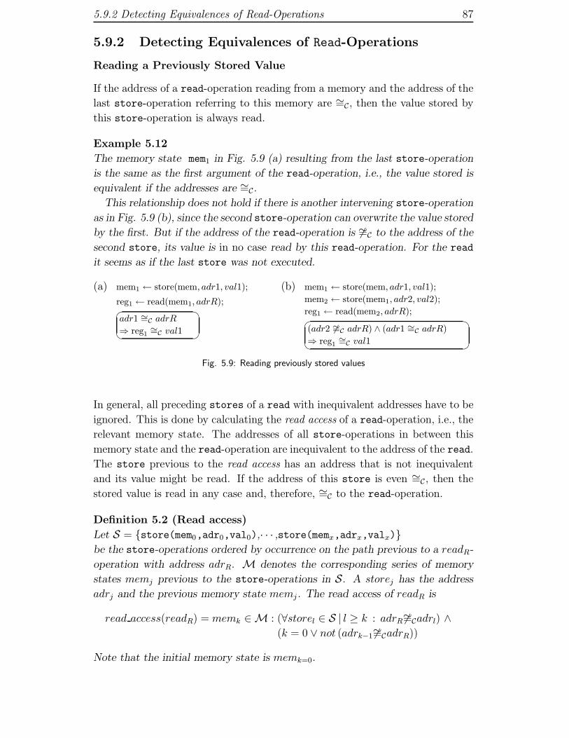
5.9.2 Detecting Equivalences of Read-Operations 87

5.9.2 Detecting Equivalences of Read-Operations

Reading a Previously Stored Value

If the address of a read-operation reading from a memory and the address of the

last store-operation referring to this memory are ∼=C, then the value stored by

this store-operation is always read.

Example 5.12

The memory state mem1 in Fig. 5.9 (a) resulting from the last store-operation

is the same as the first argument of the read-operation, i.e., the value stored is

equivalent if the addresses are ∼=C.This relationship does not hold if there is another intervening store-operation

as in Fig. 5.9 (b), since the second store-operation can overwrite the value stored

by the first. But if the address of the read-operation is �∼=C to the address of the

second store, its value is in no case read by this read-operation. For the read

it seems as if the last store was not executed.

(a) mem1 ← store(mem, adr1, val1);

reg1 ← read(mem1, adrR);

��adr1 ∼=C adrR

⇒ reg1∼=C val1

(b) mem1 ← store(mem, adr1, val1);

mem2 ← store(mem1, adr2, val2);

reg1 ← read(mem2, adrR);

��(adr2 �∼=C adrR) ∧ (adr1 ∼=C adrR)

⇒ reg1∼=C val1

Fig. 5.9: Reading previously stored values

In general, all preceding stores of a read with inequivalent addresses have to be

ignored. This is done by calculating the read access of a read-operation, i.e., the

relevant memory state. The addresses of all store-operations in between this

memory state and the read-operation are inequivalent to the address of the read.

The store previous to the read access has an address that is not inequivalent

and its value might be read. If the address of this store is even ∼=C, then the

stored value is read in any case and, therefore, ∼=C to the read-operation.

Definition 5.2 (Read access)

Let S = {store(mem0,adr0,val0),· · · ,store(memx,adrx,valx)}be the store-operations ordered by occurrence on the path previous to a readR-

operation with address adrR. M denotes the corresponding series of memory

states memj previous to the store-operations in S. A storej has the address

adrj and the previous memory state memj . The read access of readR is

read access(readR) = memk ∈M : (∀storel ∈ S | l ≥ k : adrR �∼=Cadrl) ∧(k = 0 ∨ not (adrk−1 �∼=CadrR))

Note that the initial memory state is memk=0.


Equivalence of Read-Operations

Two read-operations from the specification and the implementation are equiva-

lent if their addresses and their read accesses are equivalent. The equivalence of

the read accesses guarantees that all locations of the memory where they might

read from (depending on the actual value of the symbolic address) are identical.

Example 5.13

This procedure fails in the example of Fig. 5.10 if adr1 is neither �∼=C nor ∼=Cto adrR. The first store in the implementation is not relevant for the read-

operation, if its address adrX is inequivalent to adrR. But the read accesses

of the two read-operations are not identical because of the intervening second

store with adr1. Note that if adr1 �∼=C adrR holds, the read accesses would be

both mem and if adr1 ∼=C adrR holds, val1 would be read in both cases.


mems1 ← store(mem, adr1, val1);

regs1 ← read(mems1, adrR);

memi1 ← store(mem, adrX, valX);

memi2 ← store(memi1, adr1, val1);

regi1 ← read(memi2, adrR);�� adrR �∼=C adrX ⇒ regs1∼=C regi1

adr1 is assumed to be neither �∼=C nor ∼=C to adrR

Fig. 5.10: Equivalence of two read-operations

A supplementary check for two read-operations with equivalent addresses is pro-

vided to cope with mismatching read accesses. If the stored value and the address

of the “intervening” store-operations are equivalent, then the read access is cal-

culated again for both read-operations without these stores. This process can be

repeated until either equivalent read accesses are found, i.e., the read-operations

are equivalent, or intervening store-operations are reached that have not equiv-

alent addresses/stored values. Note that the memory states of the intervening

store-operations do not need be equivalent, see the example in Fig. 5.10.

Re-Checking Read-Operations

Our equivalence detection considers that the equivalence of the arguments of two

terms is in most of the cases already obvious, when the second term is found on

the path, see section 4.2. Therefore, it is sufficient to check only at the first

occurrence of a term whether it is equivalent to some previously found term.

Frequently, not all equivalences and inequivalences concerning the addresses

are already stated when finding read-operations for the first time on a path.

This is common for memory operations since often a value is speculatively read

or stored. An address conflict is checked afterwards to decide whether the spec-

ulation failed or not.

5.9.3 Detecting Equivalent Memory States 89

Example 5.14

The value of x is forwarded in Fig. 5.8 if there is an address conflict. If there

is no conflict, equivalence of the read-operation in the specification and in the

implementation is only obvious after the case-split setting adr1 �∼=C adr2.

Decisions about addresses later on a path as in Example 5.14 are frequent for

processor designs with pipelining. A value is read speculatively and used only if

there is no data conflict. Otherwise the relevant value is forwarded. The example

indicates, that it is important to check read-operations whenever the EqvClasses

of the corresponding addresses are modified. Therefore, the read-operations

found during symbolic simulation on a path are marked at the EqvClasses of their

addresses as dependent read-operations. If there is a change of an EqvClass,

either because it is unified or set inequivalent to another EqvClass, all dependent

read-operations are checked again, see also section 4.3. In the example of Fig.

5.8, the read-operation in the specification is marked at the EqvClass of adr2.

The equivalence of the read-operations is detected, when setting the EqvClasses

of adr1 and adr2 inequivalent.

5.9.3 Detecting Equivalent Memory States

Detecting the equivalence of two memory states is necessary to demonstrate

computational equivalence but also required to argue about the equivalence of

two read-operations in the specification and in the implementation. Finding

equivalent memory states is the same as detecting equivalent store-operations,

since a store-operation returns the whole new memory state.

Identical Order of Store-Operations

For some designs, the order of store-operations is identical in the two descrip-

tions to be compared. A sufficient, but not necessary condition for the equiva-

lence of two store-operations and, therefore, the resulting memory states is that

the addresses, the values stored, and the previous memory states are pairwise in

the same EqvClass. This is fast to test and, therefore, checked first when finding

a new store-operation. The final values of a memory in the implementation

and in the specification depend on the last two stores on both sides, which use

the result of the previous stores as first arguments. By means of an inductive

argument, when building a list in order of appearance of the stores in the im-

plementation and in the specification, every store may have its “partner” on

the other side, if the order of store-operations is identical. The first store-

operations on both sides have the initial memory state as first argument, which

is identical.

The specification and the implementation can have also only partially identical

orders of stores, which begin from two equivalent memory states. These states

may be either the initial memory state or memory states that have been iden-


tified to be equivalent by one of the techniques described below. The partially

identical store-order ends before the first store-operation-pair, where either the

addresses or the stored values are not equivalent.

Definition 5.3 (Identical store-order)

Let Sspec = {store(memsx,adrsx,valsx),· · · ,store(memsx+n,adrsx+n,valsx+n)}Simpl = {store(memiy,adriy,valiy),· · · ,store(memiy+n,adriy+n,valiy+n)}

be store-operations in the specification and in the implementation ordered by

occurrence on the path. An identical store-order satisfies:

∀k = 0, . . . , n : adrsx+k∼=Cadriy+k ∧ valsx+k

∼=Cvaliy+kIf the memory states previous to the store-operations (memsx and memiy) are equiv-

alent then the same holds for the resulting memory states, i.e., memsx+n+1∼=C

memiy+n+1.15

The order of store-operations has to be the same in the specification and in the

implementation only with regard to the same specific memory. The interleaving

of store-operations to different memories can be arbitrary, an example is given

in Fig. 5.11.

store(dmem,adr1,val1)

store(rf,adr2,val2)


store(rf,adr4,val4)

have the same store order

for both rf and dmem



store(rf,adr2,val2)

store(rf,adr4,val4)

Fig. 5.11: Identical store-orders

Overwritten Store-Operations

An identical store-order requires an equal number of store-operations on the

current path, which is not a necessary condition for equivalence of the resulting

memory states.

Example 5.15

An additional store occurs in the implementation of Fig. 5.12. Nevertheless,

the final memory states are identical if the value stored by the second store-

operation of the implementation is in any case overwritten by the third store-

operation, i.e., if the addresses are ∼=C.

This situation can occur, for instance, if the second store is speculative, but

speculation fails and the third store is used to correct the fault. Let us assume

that val2 and valX are not ∼=C. Therefore, mems2 and memi2 cannot be in the

same EqvClass and the equivalence detection of the previous subsection will fail.

But there is no difference for the last store-operation in the implementation

if the previous memory state is memi1 or memi2. Therefore the relevant preceding

15This not a necessary condition, see below.



mems1 ← store(mem, adr1, val1);

mems2 ← store(mems1, adr2, val2);

memi1 ← store(mem, adr1, val1);

memi2 ← store(memi1, adrX, valX);

memi3 ← store(memi2, adr2, val2);�� adrX ∼=C adr2 ⇒ mems2∼=C memi3

Fig. 5.12: Example for an overwritten store-operation

memory state is calculated for equivalence checking. This is either the memory

state after the first preceding store-operation, which is not overwritten by the

new store-operation or the initial memory state.

Definition 5.4 (Relevant preceding memory state)

Let Sspec = {store(mem0,adr0,val0),· · · ,store(memx−1,adrx−1,valx−1)}be the store-operations previous to storex with the address adrx and the value

valx. M denotes the corresponding series of memory states previous to the

store-operations in S. Note that adri and vali stand for arbitrary terms, see

section 5.9.1. The initial memory state is mem0.

The relevant preceding memory state of storex is

rel prec state(storex) = memk ∈M : (∀storel ∈ S | l ≥ k : adrx∼=Cadrl) ∧(k = 0 ∨ not (adrk−1∼=Cadrx))

Two store-operations in the specification and in the implementation are equiv-

alent if the addresses, the stored values and the relevant preceding memory

states are ∼=C. This criterion copes with different number of overwritten store-

operations in the specification and in the implementation. Determining the rel-

evant preceding memory state is fast, since, again, only the information of the

EqvClasses is used. Furthermore, its calculation is only necessary if there exists

a potential “counterpart” with equivalent address and stored value.

Note that by considering overwritten stores, there are some special cases

where more than two store-operations - one of the specification and one of the

implementation - are in a single EqvClass. For instance, the memory states after

the second and the third store in the implementation in Fig. 5.12 are identical

if adr2 ∼=C adrX and val2 ∼=C valX hold.

Changed Order of Store-Operations

If the store-order is changed as in the example of Fig. 5.8 for rf and Fig. 5.13

for mem, then the final memory states can be equivalent, if the addresses of the

store-operations are �∼=C. A correct reordering of store-operations can be the

result, for example, of synthesizing designs with data mapping, see section 5.9.1.

When a new store-operation is found and all previous checks fail, there might

exist a store in the other description with equivalent address and stored value,

which is the “counterpart” in a changed store order. Since the new store is


the most recent in its description, there must be some store-operations before

it, which happen after the “counterpart” in the other description.


As mems1 ← store(mem, adrA, . . . );

O1s mems2 ← store(overwritten later);

Bs mems3 ← store(mems2, adrB, . . . );

O2s mems4 ← store(overwritten later);

Cs mems5 ← store(mems4, adrC, . . . );

Ds mems6 ← store(mems5, adrD, . . . );

Ai memi1 ← store(mem, adrA, . . . );

Di memi2 ← store(memi1, adrD, . . . );

Ci memi3 ← store(memi2, adrC, . . . );

O3i memi4 ← store(overwritten later);

Bi memi5 ← store(memi4, adrB, . . . );

�� (adrD �∼=C adrC) ∧ (adrD �∼=C adrB) ∧ (adrB �∼=C adrC) ⇒ mems6∼=C memi5

Fig. 5.13: Changed order of store-operations

Assume that the new store is Ds and the “counterpart” Di in Fig. 5.13. The

stores B and C are before D in the specification but after D in the implementation.

The stores O1, O2, O3 are overwritten by subsequent store-operations, i.e.,

Bs, Cs, Ds, or Bi. A valid reordering of the store-operations requires that the

addresses of D on the one hand and B, C on the other hand are �∼=C. But we

do not know that only B and C have to be checked, since there might be some

overwritten stores O1s, O2s, or O3i in between or before B or C (see Fig. 5.13).

For a quick test, first two sets containing all memory states previous to Ds/Di are

determined, where all store-operations after those memory states and before

Ds/Di have a determined address relationship; i.e., the addresses of those store-

operations must be either �∼=C to the address of Ds/Di or ∼=C to the address of one

of the subsequent store-operations. A changed store-order is only checked, if

there are equivalent memory states in those two sets calculated for Ds and Di. In

the following, this is called that Ds and Di have a common access state, a formal

definition is given on page 93.

The next step is to determine the two sequences S1 and S2 containing the same

store-operations appearing in the two descriptions in changed order. This is not

obvious since only the end of S1 and the beginning of S2 are known. Further-

more, overwritten stores have to be considered correctly, i.e., S1 = {Bs, Cs, Ds}and S2 = {Di, Ci, Bi} in Fig. 5.13. We assume in the following that all store-

operations of the changed store-order have already appeared first in the imple-

mentation (Di to Bi) and now the last store of the opposite sequence storeS1end is

detected during the simulation, i.e., Ds. This is the first time where again equiv-

alent memory states can be reached. Since Ds is the most recent store detected

during simulation, the algorithm assumes that this is the last element missing

and that it is the end of S1. Tracing back from this point, the first (previous)

memory state is searched, which has an equivalent counterpart in the other de-

scription, i.e., mems1 and memi1 in Fig. 5.13. All preceding stores do not have to be

considered since they lead to an equivalent memory state in the implementation

and in the specification. The store-operations in the two descriptions directly


after this equivalent memory state storeS1begin (O1s) and storeS2begin (Di) are the

beginnings of S1 and S2 before eliminating overwritten store-operations.

Overwritten stores can be removed easily in S1 since the latest storeS1end(Ds) is known. Tracing back from storeS1end (Ds) to storeS1begin (O1s), all store-

operations with an address which is ∼=C to the address of a subsequent store are

eliminated, which results in S1 = {Bs, Cs, Ds}.The end storeS2end of the sequence S2 is unknown, which makes eliminating

overwritten store-operations harder. Symbolic simulation may have already

reached some store-operation after Bi which overwrites, for instance, Ci but has

to be ignored to determine S2 correctly. All store-operations after the unknown

final storeS2end (Bi) do not have to be considered when eliminating overwritten

stores in S2. S2 is determined by beginning with storeS2begin and adding suc-

cessively subsequent stores. Every time a new store is added, possibly over-

written stores are eliminated. This process is stopped, when the number of

store-operations in S2 is the same as in S1.Finally, it is controlled, if every store-operation in S1 has its partner in S2 with

∼=C address, ∼=C stored value and common access state (see above and Definition

5.5 below). In this case, the memory states after storeS1end and storeS2end, i.e., Ds

and Bi are equivalent. Note that the technique described in this section is not

limited with respect to the length of the changed store order, which is three in

our example.

The handling of some exceptional situations is not discussed in this work for

brevity. Consider for example that a store Ei follows directly Bi, which overwrites

Ci with exactly the same value as Ci. Ds is then not only equivalent to Bi but also

to Ei. This is detected by building two sequences S2a and S2b with Bi and Ei as

last elements in this special case.

The following definition gives the conditions of a valid changed store-order.

Note that the identification of such an order by the symbolic simulator as de-

scribed by the previous example is optimized with respect to computation time.

Definition 5.5 (common access state, valid changed store order)

Let

Sw/o overwritspec = {store(memsx,adrsx,valsx),· · · ,store(memsx+n,adrsx+n,valsx+n)}Sw/o overwritimpl = {store(memiy,adriy,valiy),· · · ,store(memiy+n,adriy+n,valiy+n)}

be store-operations in the specification and in the implementation ordered by

occurrence on the path. All overwritten store-operations are previously elimi-

nated, i.e.,

Sw/o overwritspec = remove overwritten(Simpl)Sw/o overwritimpl = remove overwritten(Sspec)remove overwritten(S) = {storek ∈ S :� ∃storel ∈ S | l > k : adrk∼=Cadrl}


M denotes the corresponding series of memory states previous to the store-

operations in a series S. Let memj , adrj, and valj be the previous memory

state, the address, and the value of storej . The set of access states of storez in

an order of store-operations S is:

access(storez) = {memk ∈M : ∀storel ∈ S | z > l ≥ k :

adrl∼=Cadrz ∨ adrl �∼=Cadrz}

Two store-operations of the specification storesm and of the implementation

storein have a common access state if:

common access(storesm, storein) =

∃memsk ∈ access(storesm), memi

l ∈ access(storein) : memsk∼=Cmemi

l

Note that memj denotes the memory state previous to a storej. If the store

order of Sw/o overwritspec and Sw/o overwritimpl are not identical according to Definition 5.3

then a valid changed store order is given if:

∀storesk ∈ Sw/o overwritspec : ∃storeil ∈ Sw/o overwritimpl :

(adrsk∼=Cadril) ∧ (valsk

∼=Cvalil) ∧ common access(storesk, storeil)

If the memory states previous to the store-operations16 are equivalent then the

same holds for the resulting memory state, i.e., memsx+n+1∼=C memiy+n+1.

5.9.4 Summary

Symbolic simulation has to cope with two aspects concerning memories: first, the

in general large sizes of the memories. We argue only about memory operations,

i.e., store- and read-operations. Therefore, the size of the memories is irrelevant,

but the symbolic simulator has to detect equivalences of the memory operations

in order to model correctly the behavior of the memory.

Second, indirect addressing has to be considered. This makes necessary a rea-

soning process about the relationships of the addresses during symbolic simula-

tion, since they can be arbitrary symbolic terms. Collecting equivalent symbolic

terms in EqvClasses permits us to establish a fast address comparison for our

memory-specific equivalence detection methods. The symbolic simulator copes

with complex reorderings of memory operations as demonstrated also by the

experimental results presented in section 7.1.

16Which need not be memsx and memiy since the first store-operations might be overwritten,

i.e., Sspec/impl are relevant instead of Sw/o overwritspec/impl .

5.10 Inequivalences Forcing Terms to be Constant 95

5.10 Inequivalences Forcing Terms

to be Constant

Inequivalences can force a term to be constant. Since the domain of a n-bit-vector

is restricted to 2n values, setting it �∼=C to 2n−1 values implies equivalence to the

remaining value. Fig. 5.14 (a) gives an example for a bit-vector, where b�∼=C10and b�∼=C00 and b�∼=C11 ⇒ b ∼=C01 holds. Note that there can be intervening

assignments and other conditions in Fig. 5.14.

(a) if b="10" then ...

elsif b="00" then ...

elsif b="11" then ...

else � ��b="01" is true

(b) if a[3] then

if a[2:1]="11" then ...

elsif a[2:1]="10" then ...

else � ��a[3:2]="10" is true

Fig. 5.14: Terms being constant due to decided inequivalences

Two EqvClasses are inequivalent either because of a decision in a case split

or since they contain different constants which is not relevant here. Check-

ing after each decision whether the EqvClass is set inequivalent to 2n − 1 con-

stants is not sufficient. Also decisions about parts of a term have to be consid-

ered, see Fig. 5.14 (b) where a[3]∼=C1 and a[2:1]�∼=C11 and a[2:1]�∼=C10 ⇒a[3:2]∼=C10 has to be detected. Moreover, it is not relevant in this example

whether the entire term a is equivalent to a constant but only the bits a[3:2].

Two counters ctrl-zero-bit and ctrl-one-bit are introduced for each bit of a term

appearing in conditions. They are initialized during pre-processing with 2N−1

where N is the length of the term (not 2N − 1!). A bit i of a term is equivalent

to 0 (1) if ctrl-zero-biti (ctrl-one-biti) is zero. The counters are decremented if:

• the term is set inequivalent to a constant. ctrl-one-bit and ctrl-zero-bit are

decremented at all bit-positions, where this constant is 0 or 1, respectively;

a table supports determining the relevant bit-positions for constants ap-

pearing explicitly in the descriptions since all constants are expressed as

integers during simulation, see section 4.3;

• a bit-selection of a term is set inequivalent to a constant. Not only the ctrl-

one-bit- and ctrl-zero-bit-counters of the term representing the bit-selection,

e.g., a[2:1] are decremented but also the corresponding counters of the

entire term a are decremented according to the size of the bit-selection.

Multiple selections, e.g., (a[10:2])[2:1] are considered by recursion.

Every time a new constant bit is found it is checked whether the whole term

is constant, too. The equivalence of the bit has to be marked if this test fails.

If there exists a term representing the bit-selection of the relevant bit then the

corresponding EqvClasses are unified. Otherwise equivalence of the bit to the

constant 0 or 1 is marked directly at the term.

Chapter 6

Using Decision Diagrams to

Detect Equivalences

Section 6.1 gives an overview of the dd-checks. The construction of formulas

which demonstrate the equivalence to be verified is described in section 6.2.

Checking those formulas by vectors of OBDDs is compared to other techniques

in section 6.3. The use of intermediate dd-checks for gate-level simulation is

presented in section 6.4. Section 6.5 discusses how the decisions of conditions

are considered during a dd-check. The results of a dd-check are reused during

the following symbolic simulation of the remaining paths which is described in

section 6.6.

6.1 Overview

The equivalence detection techniques presented in the previous chapter are not

complete in order to provide a fast symbolic simulation. Therefore, checking

the verification goal by a test for equivalence at the end of a path (line 11

in Algorithm 4.1) may fail. The more accurate tests called dd-checks based on

decision diagrams are used at the end of a path in these cases. They have to reveal

whether (i) computational equivalence is given in this path but was not detected

(line 16), (ii) a condition has been decided inconsistently due to the incomplete

equivalence detection on the fly (line 19), or (iii) a valid counterexample can be

given (line 22).

Decision diagrams are used in the dd-checks to reveal special equivalences

which are not considered by the techniques presented in the previous chapter

either since they occur seldom or because they are hard to detect. Examples are

given in section 6.4, 6.5, and 7.3. Two tests are provided:

• testing whether two terms are equivalent; note that checking the validity

of a condition is the same as comparing it to the constant 1;

• testing whether a term is equivalent to a constant; this is a different case

since the value of the constant is unknown.

97

98 CHAPTER 6 Using Decision Diagrams to Detect Equivalences

A formula demonstrating the equivalence is built for each test considering knowl-

edge about path-dependent equivalences or inequivalences of intervenient terms.

The Multiple-Domain Decision Diagram Package (the TUDD-package) [Hor99,

Hor97, Hor98] developed at Darmstadt University of Technology with an exten-

sion for vectors of OBDDs is used to prove the formula. Each graph represents

one bit of the two terms to be compared. The extension developed for the

symbolic simulator permits to apply functions to vectors of OBDDs instead of

manipulating separately single decision diagrams.1 Therefore, the formula con-

sisting of function applications to bit-vectors is checked automatically by the

TUDD-package without additional modifications. It is tested whether a similar

formula has been built previously and stored in a hash-table before applying

vectors of OBDDs.

The dd-checks testing the verification goal at the end of the path may fail if

a false path is reached. All decided conditions (i.e., CondBits in C for which a

case-split was performed) are checked in order of their occurrence in this case to

search for a contradictory decision due to the incomplete equivalence detection

on the fly. Using the information of the equivalence classes again facilitates

considerably the construction of the required formulas.

A path is backtracked if at least one formula is valid (line 16 in Algorithm

4.1) or if a contradictory decision has been detected (line 19). Moreover, the

relationship revealed by the dd-check is marked as described in section 6.5 so

that it is checked during symbolic simulation of the remaining paths. Otherwise

a valid counterexample is found which is reported for debugging.

Section 4.6 motivated the use of intermediate dd-checks at gate-level also dur-

ing the path search (line 9 in Algorithm 4.2) instead of using them only at the

end of a path. The intermediate tests are discussed in section 6.4.

The dd-checks do not make the equivalence detection complete, since some

functions like multiplication or memory operations are not interpreted during the

dd-check to avoid extensive computation times and/or graph explosion. These

terms are represented by dd-cutpoints (described in the next section) during

OBDD-construction. Additional dd-cutpoints are used to speed up the dd-checks.

In spite of these simplifications, the dd-checks provide a substantial improvement

of the equivalence detection. No corner-case has been found during our experi-

ments which was not detected by the implemented dd-checks. Note that the dd-

checks need not be incomplete in principle in our symbolic simulation approach.

The incompleteness is caused by the dd-cutpoints which are only introduced be-

cause of the practical limitations of current OBDD-packages.

1For example, the application of the function ADD to two vectors of OBDDs {a0, . . . , an}and {b0, . . . , bn} is implemented using the basic functions and, or, and xor of the TUDD-

package. The result is another vector of OBDDs.

6.2 Building Formulas in dd-checks 99

6.2 Building Formulas in dd-checks

The support of two terms has to be the same if the equivalence of the terms is

tested using decision diagrams. This can be achieved by backward-substitution

so that only initial RegVals, which are identical in the specification and in the

implementation, or constants occur on each side. Note that the formula is less

complex than a formula describing the entire verification problem since a specific

path is chosen. However, a complete backward-substitution is not efficient since

only the information about the path is used but not about equivalences detected

by the other techniques. For example, if both terms depend only on two interme-

diate RegVals detected previously to be equivalent, it makes sense to introduce

a dd-cutpoint and to consider this dd-cutpoint as primary input: all expressions

or assignments previous to this dd-cutpoint do not have to be considered in the

decision diagrams.

Therefore, first the two sets representing all EqvClasses of the intermediate

terms are collected in a fast backtracking. The intersection of those two sets

of EqvClasses represents the candidates for dd-cutpoints. Any term with an

EqvClass in the intersection is represented by a dd-cutpoint when constructing

the formula by backward-substitution, i.e., the dd-check considers this term as a

primary input just as the initial RegVals.

The dd-cutpoints have to be removed in some cases since they hide subterms

which are required to demonstrate equivalence, see section 6.4 for an example.

Therefore, a failed dd-check is repeated without dd-cutpoints.

Another possibility to obtain a simpler formula is to replace a term during

formula construction by another term in the same EqvClass. Again, the results

of the previous symbolic simulation are used. Replacing a term by another term

in the same EqvClass is useful if the corresponding representation as decision

diagram is simpler. For example, if a term is in an EqvClass with a constant, then

only the OBDD for the constant is constructed. A simple heuristic counts the

expected complexity concerning graph construction of each term in the EqvClass

of a term. The term with the lowest complexity is used as representative for the

EqvClass, i.e., it replaces the other terms in the dd-check.

Replacing terms by other terms in the same EqvClass or by dd-cutpoints can

be misleading if the consistency of the decided CondBits is verified, i.e., if it

is checked whether a false path is reached (line 19 in Algorithm 4.1). If the

condition of an inconsistent CondBit establishes an equivalence of two terms,

then replacing the terms by a dd-cutpoint or one of the terms by the other term

makes detecting the inconsistency infeasible. Therefore, all EqvClasses with a

term appearing in the condition of a subsequently decided CondBit have to be

ignored when checking the consistency of a decided CondBit. Terms in such a

EqvClass are replaced neither by dd-cutpoints nor by other terms of this EqvClass.

A hash-table is used to avoid building identical decision graphs repeatedly in


different dd-checks. The result of a previous dd-check can be reused even if the

two formulas of the dd-checks are not identical. The same formula may be built

in the new dd-check with only different RegVals or dd-cutpoints. Therefore, all

RegVals and dd-cutpoints are replaced in order of their appearance in the formula

by auxiliary variables T1, T2,...,Tn before hashing a formula. New formulas are

checked using vectors of OBDDs and the result is hashed.

Note that a verification using only vectors of OBDDs without considering re-

sults of the symbolic simulation is neither efficient nor feasible for large examples,

see section 7.3. A small example for the simplification of a formula in a dd-check

by using results of the other equivalence detection techniques is given in Fig.

4.14 in section 4.5.2.

6.3 Comparison to Other Approaches

for Formula-Checking

A dd-check consists of extracting first a formula which is valid if the two terms to

be compared are equivalent and then verifying this formula by means of vectors

of OBDDs. The formula established could be verified also by other techniques.

Two of them are compared in our domain of application to vectors of OBDDs

in the following: another type of decision diagrams and a specialized formula

checker called SVC, see section 3.3. Note that techniques which require possibly

user-interaction to check a formula, e.g., theorem-provers are not suited for our

automatic verification approach.

A different possibility to represent and check a formula is to use word-level

decision diagrams like *BMDs [BC94, BC95] instead of vectors of OBDDs. Bit-

selections are used frequently in practical examples of control logic, either ex-

plicitly, e.g., R[13:16], or implicitly, e.g., storing the result of an addition in

a register without carry. Using *BMDs, terms are represented by one single

*BMD. Bit-selection, therefore, requires one or two modulo-operations which are

worst-case exponential with *BMDs.

Bit-selection is quasi for free, if terms are expressed as vectors of OBDDs,

where each graph represents one bit. Bit-selection can then be done by simply

skipping the irrelevant bits, i.e., the corresponding OBDDs and by continuing

computation with the remaining graphs. Checking equivalence just consists of

comparing each bit-pair of the vectors.

All previously applied equivalence detection techniques are (fairly) indepen-

dent of the bit-vector length. Results obtained during symbolic simulation are

used to simplify formulas before OBDD-vector construction. But even without

simplification, large bit-vectors can be handled by OBDD-vectors in acceptable

computation time.

The results of SVC on five bit-vector arithmetic verification examples are com-

pared in [BDL98] to the results of the *BMD package from Bryant and Chen

6.3 Comparison to Other Approaches for Formula-Checking 101

and also to Laurent Arditi’s *BMD implementation which has special support

for bit-vector and Boolean expressions. We verified these examples also with

OBDD-vectors. Tab. 6.1 summarizes the results. All our measurements are on

a Sun Ultra II with 300 MHz. Various orderings of the variables for our *BMD-

measurements are used; the best results are reported. The line DM contains

additional verification results for a bit-wise application of De Morgan’s law to

two bit-vectors a and b, i.e., a0 ∧ b0&...&an ∧ bn ≡ (a0 ∨ b0)&...&(an ∨ bn), and

the ADD-example is the verification of a ripple-carry-adder. Note that the input

for the two last examples is also one word and not a vector of inputs. Otherwise

*BMD-verification is of course fast since no bit-selection or modulo operation is

required. The inputs may represent some intermediate cut-points for which, e.g.,

the *BMD is already computed.

*BMD *BMD OBDD-vectorSVC1

Bryant/Chen1 Arditi1 TUDD

200MHz 200MHz 300MHz 300MHz Sun Ultra II

Pentium Pentium UltraSparc 30

Bits 16 32 16 32 16 32 16 32 64 128 256

1 N/A 0.002 N/A N/A N/A 0.04 0.14 0.27 0.38 0.68 1.38

2 N/A 0.002 N/A N/A N/A 1.10 0.13 0.20 0.25 0.44 0.93

3 0.002 0.002 265.0 >500 0.07 0.18 0.21 0.32 0.51 0.95 1.95

4 0.002 0.002 26.4 >500 0.72 8.79 0.24 0.40 0.71 1.53 4.38

5 0.111 0.520 22.7 >500 0.39 3.78 0.14 0.21 0.31 0.57 1.15

Measured at Measured with

TUDD TUDD *BMD-package

Bits 16 32 16 32 64 16 32 64 128 256

DM >5min >5min 0.12 0.22 0.28 0.48 1.03

ADD -2 5.19 37.2 282.7 0.21 0.31 0.48 0.98 1.901 Measurements reported in [BDL98].2 2 Bit: 1.01s; 4 Bit: 9.47s; 5 Bit 44.69s; Verification with more than 5 Bit was

not feasible with the current version of SVC.

Tab. 6.1: Comparison of SVC, *BMD and OBDD-Vectors. Times are in seconds

Obviously, *BMD-verification suffers from the modulo-operations in the ex-

amples. According to [BDL98], the results of example 1 to 4 are independent

of the bit-vector length for SVC, but the verification times with OBDD-vectors

are also acceptable even for large bit-vectors. These times can be reduced espe-

cially for small bit-vectors by optimizing our formula parsing. In example 5, SVC

ends up slicing the vector. Thus the execution time depends on the number of

bits and shows, therefore, a significant increase, whereas the computation time

for OBDD-vectors increases only slightly. The increase in this example may be

eliminated in a future version of SVC [BDL98], but the general problem is that

slicing a vector has to be avoided in SVC. This is demonstrated by the examples

DM and ADD, where verification is only practical with OBDD-vectors.

Note that functions that are worst-case exponential with OBDDs, e.g., multi-

plication or which have no representation are only problematic in rare cases where


special properties of the functions are necessary to show equivalence. Normally,

these terms are replaced by dd-cutpoints during formula-construction since in-

formation from the other equivalence detection techniques is used.

6.4 Comparing Descriptions

at RT- and Gate-Level

Section 4.6 motivated the use of intermediate dd-checks during the path search if

one of the descriptions is at gate-level instead of using them only at the end of a

path (line 9 in Algorithm 4.2). The same entire Boolean expressions assigned to

the register bits have to be simulated at gate-level in each symbolic simulation

cycle. It is crucial to find relationships of the control registers in the previous cycle

in order to detect equivalences in the next cycle between the Boolean expressions

at gate-level and the much simpler corresponding terms in the specification at

algorithmic- or rt-level. Usually, the control registers appear frequently in the

Boolean expressions. The equivalence detection techniques presented in section

5.2 can often neglect subterms or decide equivalences if information is provided

about the value of the control registers.

Example 6.1

The register cnt in Fig. 6.1 is assumed to be a microprogram counter and

the assignments to all registers depend on the value of this control register.

The assignment to cnt is represented at gate-level by a concatenation (&) of

the single bits. Only the expression of one bit is shown in Fig. 6.1. This bit

Specification

if ak[3:0]=mi[3:0]

then ...

else selected branch;

Implementation

cnti1 ←bitn &...&

((ak[3] xor mi[3]) nor (ak[2] xor mi[2])) and

((ak[1] xor mi[1]) nor (ak[0] xor mi[0]))

&...& bit0;

Fig. 6.1: Example for the advantages of intermediate dd-checks

is constant since ak[3:0]�∼=Cmi[3:0] ⇒ ((ak[3] xor mi[3]) · · ·(ak[0] xor

mi[0])) ∼=C 0 which is not revealed without dd-check by the other equivalence

detection techniques.

Detecting that the (controlling) microprogram counter is equivalent to a con-

stant is important, since the assignments to all registers in the next cycle are

identified to be equivalent to a corresponding RegVal in the specification in this

case. Otherwise the ”link” between terms in the specification and in the imple-

mentation gets lost not only in the next cycle but also in all subsequent cycles

since the respective preceding RegVals are used as arguments. A final dd-check

would be complex since the subsequent cycles have to be considered in the de-

cision diagrams additionally before equivalent terms of the specification and of

the implementation are reached.

6.4 Comparing Descriptions at RT- and Gate-Level 103

Losing the ”link” is avoided by providing an intermediate dd-check at gate-

level if no equivalence has been found for a term assigned to a RegVal. This

intermediate dd-check reveals in Example 6.1 that cnti1 is equivalent to 0.

An intermediate check is provided for a RegVal in the description at gate-level

if the following conditions hold:

• no equivalence between the term assigned to the RegVal and any other

term has been detected by the other equivalence detection techniques;

• the register is not excluded from intermediate dd-checks; the user can limit

the application of intermediate dd-checks on relevant control registers; this

(easily provided) information is optional, but can decrease simulation time

significantly.

The dd-check requires an assumption about which term might be equivalent to

the intermediate RegVal ix. If the register does not exist in the specification, e.g.,

a control register of the hardware implementation, it is only checked

• whether the term is equivalent to a constant. The OBDD-vector of the

term is built using each RegVal of the previous cycle as dd-cutpoint. If each

bit of the OBDD-vector is equivalent either to 0 or 1, then the constant

result of the term is calculated;

• if the term has not changed in the last step, i.e., RegVal ix∼=CRegVal ix−1

Otherwise equivalence to the first corresponding RegVal sy in the specification

(with the lowest y) is checked, which is neither equivalent to some term of the

implementation nor to some initial RegVal. Consider first the case that the

preceding RegVal ix−1 in the implementation has an equivalent ”counterpart” in

the specification. In this case, all RegVals of the preceding cycle are used as

dd-cutpoints in the implemenation during the dd-check. But equivalent terms

might be reached in the specification and in the implementation after different

numbers of cycles.

Example 6.2

xs1 ←a+b+c in the specification is calculated in two cycles by xi1 ←a+b and

xi2 ←xi1+c in the implementation. Only xi2 has an equivalent counterpart in this

case. The dd-check cannot reveal this fact if the dd-cutpoints are set to the

previous cycle, i.e., xi1.

Therefore, a failed dd-check is repeated with the dd-cutpoints shifted succesively

to the preceding cycle until either the dd-check is satisfied or the RegVal of the

relevant register in the implementation has an equivalent counterpart in the

specification. Note that equivalence would be revealed in the simple Example

6.2 used for illustration without dd-check by the other equivalence detection

techniques described in chapter 5.


6.5 Considering Previous Decisions

A case-split is performed each time the value of a condition is not determined

by the acceptable initial values of the registers. The decision is reflected in the

EqvClasses and is, therefore, considered by the equivalence detection techniques

during the symbolic simulation as well as during formula construction in a dd-

check. There remain cases where the decisions have to be considered separately.

Example 6.3

The equivalence of the final values of res in Fig. 6.2 is not detected without

dd-check since none of the bits of the bit-vector m is constant. The dd-check has

to consider the inequivalences of m and the four constants to reveal that the least

significant bit of res is equivalent to 0 (see box in Fig. 6.2).

Specification

if m=0110 or m=0011 then ...

elsif m=0010 or m=0111 then ...

else ress1 ← b[31 : 1]&0;

Implementation

resi1 ← b[31 : 1]&((not m[3]) and m[1]);

��(m �∼=C0110) and (m �∼=C0011) and (m �∼=C0010) and (m �∼=C0111)

⇒ ((not m[3]) and m[1])∼=C0

Note that none of the bits of m is constant. m is declared m[3:0]

Fig. 6.2: Considering decisions in a dd-check

Therefore, every dd-check which failed to demonstrate a formula F is repeated

considering decisions about conditions which share terms with the formula. Con-

ditions from CondBits which have no terms in common with the formula can have

no impact on the check. The conditions of the relevant CondBits are combined by

conjunction. Conditions of CondBits which are decided to be false are considered

negated, see Equation 6.1.

decrel =∧

i∈relevantCondBits

{cond of(i) : if value(i) = true

not (cond of(i)) : if value(i) = false(6.1)

Note that only previous decisions are considered for intermediate dd-checks de-

scribed in section 6.4. The repeated dd-check tests whether decrel ⇒ F holds.

If it is only checked whether a term is equivalent to a constant, the test has to

be refined. No F is provided since the constant is unknown. But each bit has to

be equivalent to a constant. Therefore, it is checked if decrel implies that each

bit of the term is either 0 or 1:

∀k ∈ bits of term :[decrel ⇒ dd of(k)

]or[decrel ⇒ not (dd of(k))

](6.2)

If there exists an equivalent constant, then it is calculated during the check of

Equation 6.2. Note that accessing dd of(k) is for free using vectors of OBDDs.

6.5 Considering Previous Decisions 105

When building the formula for the dd-check, terms are often represented by

dd-cutpoints or by other (simpler) terms in the same EqvClass. For example, if a

term is in an EqvClass with a constant, then only the OBDD for the constant is

constructed. However, these replacements have to be considered when including

previous decisions.

Example 6.4

Fig. 6.3 (a) extends the example of Fig. 6.1 by an assignment irs1 ←ak[1:0]

and a condition testing irs1 =”10”.

(a)

Specification

irs1 ← ak[1:0];

if irs1="10" then

if ak[3:0]=mi[3:0]

then ...

else selected branch;

Implementation

cnti1 ←bitn &...&

((ak[3] xor mi[3]) nor (ak[2] xor mi[2])) and

((ak[1] xor mi[1]) nor (ak[0] xor mi[0]))

&...& bit0;

(b) Formula used for checking if cnti1 is equivalent to 0

ak[3:0] �∼=C mi[3:0] ⇒((ak[3] xor mi[3]) nor (ak[2] xor mi[2])) and ;;not valid

((1 xor mi[1]) nor (0 xor mi[0]))∼=C0

Note: irs1 does not appear in the formula

(c) Refined decrelrefined (see below) permit to obtain correct result

(ak[3:0] �∼=C mi[3:0]) and (ak[0]∼=C0) and (ak[1]∼=C1) ⇒((ak[3] xor mi[3]) nor (ak[2] xor mi[2])) and ;;valid

((1 xor mi[1]) nor (0 xor mi[0]))∼=C0

Fig. 6.3: Refining the decisions considered in a dd-check

The constants 1 and 0 are simpler to represent than the equivalent terms ak[1]

and ak[0]. Therefore, the constants replace those terms in the dd-check (see Fig.

6.3 (b)). But the formula in Fig. 6.3 (b) is not valid. Note that irs1 does not

appear in the formula even before replacing ak[1] and ak[0] by 1 and 0.

The calculation of decrel has to consider that

• only one representative may be used for terms of the same equivalence

class, i.e., the same vector of OBDDs is used and that

• decisions about the equivalence of a term (e.g., irs1 in Fig. 6.3 (a)) can

establish equivalences of some bits of another term (ak). Therefore, decrel

is also refined if a term in a bit-selection is represented in the formula of

the dd-check by another term or by a dd-cutpoint.

The calculation of decrelrefined is given in equation 6.3.

decrelrefined = decrel ∧ ∧termi∈R

termi∼=C repr(EqvClass(termi))

(6.3)


The set R contains all terms or bit-selections of terms which satisfy:

• the term has been replaced by a term of the same EqvClass or by a dd-

cutpoint during formula construction, i.e., it is represented in the dd-check

by repr(EqvClass(termi)), and

• one of the terms in the conditions of the relevant CondBits is either equiv-

alent to the term or - if the term is a bit-selection - to the argument of the

bit-selection.

Fig. 6.3 (c) describes how the correct result is obtained using decrelrefined.

6.6 Reusing Results of a dd-check

The result of a dd-check is also used in the following symbolic simulation of

the remaining paths. It is likely that also in other paths a dd-check is invoked

again to verify the same formula, which should be avoided. The corresponding

decision diagram will be not built again since formulas are hashed as described in

section 6.2. However, detecting the equivalence of the two terms already during

simulation is more efficient since this information can be used to detect other

equivalences and to avoid false paths.

The EqvClasses of the two terms tested for equivalence in the dd-check cannot

be unified directly: the dd-check verified their equivalence only concerning the

set of possible initial RegVals on a given path. Decisions resulting from case-

splits might be considered in the dd-check. Furthermore, terms can be replaced

by dd-cutpoints or by other equivalent terms for the construction of the decision

diagrams. The following conditions have to be satisfied to reuse the result of a

dd-check:

• the values of the CondBits considered in the dd-check must be the same,

• all terms which are replaced by the same dd-cutpoint in the dd-check are in

the same EqvClass, and

• if a term is replaced by another equivalent term in the dd-check then those

two terms must be once more in the same EqvClass.

These conditions and the equivalence they imply are the result of the dd-check.

Verifying if the conditions hold is fast during the following simulation of the

remaining paths, since only values of CondBits are reviewed and EqvClasses are

compared. The conditions are checked whenever

• one of the two terms compared in the dd-check is found,

• one of the terms (except constants) which must be equivalent to other

terms is found or its EqvClass is unified with another EqvClass, or

6.6 Reusing Results of a dd-check 107

• one of the CondBits considered is decided.

The EqvClasses of the terms compared in the dd-check are unified if the corre-

sponding conditions are satisfied.

Chapter 7

Experimental Results

Symbolic simulation has been applied to demonstrate computational equivalence

of descriptions at different levels of abstraction:

• behavioral-rtl against behavioral-rtl: automatically constructed pipelined

processors are compared to the corresponding specifications of the DLX-,

Alpha,- and PIC-instruction set. The results in section 7.1 demonstrate

that our symbolic simulator copes with distinct orders of memory opera-

tions in the two descriptions to be compared;

• behavioral-rtl against structural-rtl: the verification of a structural de-

scription of a microcontroller against two behavioral specifications is pre-

sented in section 7.2; furthermore, experimental results for the verification

of pipelined DLX-processors with different implementation details are re-

ported;

• rt-level against gate-level: descriptions at gate-level synthesized by the

Synopsys©R Design CompilerTM using the AlcatelTM MTC45000-library are

compared to specifications at behavioral rt-level.

Note that most of the experiments required a sequential verification, e.g., equiv-

alence of the descriptions at gate- and rt-level is only given after several control

steps.

The scope of the verification tool described in section 2.2 is larger than equiva-

lence checking. In particular, property verification is another possible application

area, see section 2.7. First results about an application to another verification

problem than equivalence checking are given in section 7.4 which describes reg-

ister binding verification.

109

110 CHAPTER 7 Experimental Results

7.1 Behavioral RTL against Behavioral RTL

The results of the verification of four designs are given in Tab. 7.1. In all ex-

amples, a sequential specification is compared with the corresponding pipelined

implementation. The specifications reflect a subset of the instructions of the

respective architecture, i.e., the Alpha-architecture from Digital [Cor92], the

DLX-architecture [HP96], and the PIC16C5X-processor from Microchip [Inc93].

The implementations were generated automatically from the specifications us-

ing a transformation tool developed at Darmstadt University of Technology

[Hin00, HER99, HRE99, EHR98, Hin98a, HRE00]. Note that there are consider-

able differences between our Alpha implementation and the processor produced

by Digital, e.g., concerning the number of pipeline stages. The TUD trans-

formation tool uses a small-set of correctness preserving transformations. The

descriptions are obtained automatically by gradual application of the transfor-

mations. Another application of the TUD transformation tool in addition to

pipeline synthesis is the automatic verification of scheduling results in high-level

synthesis [EHR99].

Verification of the pipelined designs was done using the flushing approach of

[BD94], see section 4.1.3 and appendix 9.8. The two acyclic finite sequences to

be compared are generated automatically. No transition function is required as

in [BD94]. The behavioral description of the pipelined system consists of several

parts, called segments, which describe different combinations of instruction stages

of the pipeline, i.e., the partially filled/flushed pipeline or the full pipeline state.

All parts have to be verified using the flushing approach. For example, 9 parts

are used to describe a DLX with 5 pipeline stages [Hin00]. The behavior of the

system if the stall-input is set or cleared, i.e., whether the pipeline is flushed or

not is separately described for each part. Therefore, automatic generation of the

two sequences to be compared (section 4.1.3) is possible by setting the stall-input

accordingly and simply linking the relevant parts until the part describing the

empty pipeline is reached. An example is given in [Hin00].

Tab. 7.1 gives the verification time, the number of instruction classes1, and

the total number of paths checked during the symbolic simulation of all parts of

the descriptions.2 Computational equivalence has been verified with respect to

the data memory, the register file, and the program counter.3 Measurements are

on a Sun Ultra II with 300 MHz.

The results demonstrate that the equivalence detection techniques described in

section 5.9 cope with distinct orders of memory operations in the two descriptions

to be compared. The sixth column shows in how many paths store-operations

1For example, the instruction classes of the DLX are direct and indirect alu-, load-, store-,

branch-, and jump-instructions.2The verification results for the different parts are aggregated in Tab. 7.1. [Hin00] reports

the results for each part separately.3The instruction memory is not written, i.e., verification is trivial.

7.1 Behavioral RTL against Behavioral RTL 111

are overwritten (section 5.9.3, pages 90 to 91). The number of paths with changed

order of the store-operations (section 5.9.3, pages 91 to 94) is given in the last

column. Paths with changed store-order are not considered in the sixth column

although stores may be overwritten in these paths, too.

The store-order in the DLX-example is always identical in the specification

and in the implementation and no overwritten stores have to be considered.

The same results have been obtained for the verification of the structural DLX-

descriptions, see section 7.2. The Alpha-example requires additionally detecting

overwritten store-operations. Consider two stores to the Alpha register file

with equivalent addresses, which are executed consecutively in the sequential

description. One of them is skipped if they are executed in different instruction

stages which are parallelized by the synthesis tool. Note that the register file of

the DLX (respectively the data memory) is always written in the same instruction

stage.

Pipeline Instruction Verification Total Paths with storesDescription

stages classes time paths overwritten changed order

DLX 5 6 46min 23s 1506698 - -

Alpha 3 10 7.84 s 2374 88 -

PIC 1 2 17 252.6 s 107655 3151 1741

PIC 2 2 17 379.6 s 161622 4338 5252

Tab. 7.1: Experimental results for behavioral rtl verification

All techniques presented in section 5.9 are required to verify the two PIC-

examples. The store-order was changed significantly in many paths after in-

troducing pipelining. The reason is the data memory mapping used by this

architecture, i.e., single registers are addressed in the same manner as registers

of the register file. Formal verification has to consider the access to registers and

register file by a single memory model, see also [Hin00] and section 5.9. The

mapping makes synthesis (and verification) more complicated since numerous

additional data conflicts have to be resolved. This is also demonstrated by the

higher complexity of PIC 2 compared to PIC 1. The only difference of PIC 1 is

that the STATUS-register is excluded from data mapping. Another reason for

the complexity of the PIC-examples compared to the Alpha- and DLX-example

(which have more pipeline stages) is the larger number of instruction classes.

The DLX-results reported in [RHE99] refer to a simpler DLX-description4 than

the results given in Tab. 7.1.

We verified the Alpha-example with the test for changed store-order switched

off and the DLX-example also without the checks for overwritten stores. Com-

putation time changed only less than one second, which demonstrates that the

overhead introduced by testing for complex read/store-schemes in the equiva-

lence detection is acceptable.

4The instruction stages are less parallelized and the description considers one instruction

class less.


Only the verification of the PIC-examples required dd-checks as described in

chapter 6 to demonstrate computational equivalence. The small set of transfor-

mations used during synthesis is considered by the other equivalence detection

techniques. The dd-checks in the PIC-example are only necessary to detect incon-

sistencies due to the varying length of the PIC instruction code.

Various implementation bugs of the synthesis tool have been revealed by the

symbolic simulator. These bugs did not concern the correctness of the transfor-

mations but only the implementation of the tool. One of the bugs which has been

detected during the verification of the behavioral DLX-processor is illustrated in

the following example.

Example 7.1

The abbreviations in Fig. 7.1 denote the instruction stages of the DLX-pipeline,

i.e., instruction-fetch- (IF), decode- (ID), execute- (EX), memory- (MEM) and

write-back-stage (WB). The error occurs iff an ALU-instruction uses both val-

R3←R1 aluop R2

LOAD R2,Y

LOAD R1,X IF ID EX MEM WB

IF ID EX MEM WB

IF ID / EX MEM WB

⇑new value of R1 not available

Fig. 7.1: Implementation bug revealed

ues loaded by two directly preceding LOAD-instructions. The execution on

the initially generated system with pipelining is described in Fig. 7.1. The

ALU-instruction is stalled until the preceding LOAD-instruction has reached

the WB-stage. The first LOAD-instruction terminates in the meantime. The

ALU-instruction has loaded in its ID-stage the old, wrong value of R1. But it is

not possible to forward the correct value in the EX-stage since the first LOAD-

instruction has terminated by writing the value of R1 into the register-file. The

synthesis tool did not detect the data dependency in an older version. Solutions

to avoid this bug are to repeat the ID-stage during the stall or to add another

pipeline register.

A practical important advantage of the symbolic simulator is its good debugging

support.

Example 7.2

The following comments about a counterexample turned out to be helpful during

the experiments reported in this section:

• a complete description of the path in specification/implementation in the

initial and/or the internal description language;

7.2 Structural RTL against Behavioral RTL 113

• the last expressions assigned to the registers and memories with and/or

without backward-substitution of expressions assigned to RegVals;

• decisions performed at case-splits, i.e., the values of decided CondBits;

additionally, a list of the values of all CondBits, i.e., including conditions

not requiring a case-split;

• equivalence of RegVals/terms to constants;

• a summary how instructions are carried through the pipeline registers;

• inequivalences of EqvClasses.

The symbolic simulator provided also useful information for the improvement of

the synthesis tool after a successful verification. Never taken branches of if-then-

else-clauses are reported after simulating symbolically all possible paths. These

branches are logically impossible and indicate redundancy of the control logic.

7.2 Structural RTL against Behavioral RTL

7.2.1 DLX-Processor Descriptions

Two implementations of a subset of the DLX processor [HP96] have been verified,

the first from [HSG98], initially verified in [BD94], and a second one designed

at Darmstadt University of Technology.5 The second description contains more

structural elements, e.g., multiplexers and corresponding control lines required

for forwarding are given. Both examples have a 5-stage pipeline with branch-

predict-not-taken strategy.6

For both descriptions, acyclic sequences are generated by using the flushing

approach of [BD94]; i.e., the execution of the inner body of the pipeline loop

followed by the flushing of the pipeline is compared to the flushing of the pipeline

followed by one serial execution. Different from [BD94] (see also [Bur96]), our

flushing technique guarantees that one instruction is fetched and executed in the

first sequence. Otherwise it has to be communicated between the specification

and the implementation if an instruction has to be executed on the sequential

processor or not (e.g., due to a load interlock in the implementation). [Bur96]

describes this as keeping the implementation and the specification in sync. How

to generate the two finite sequences to be compared using the flushing approach

of [BD94] is described for the second structural DLX-example in appendix 9.5.

5A slightly modified version of the second design has been verified, too, which is not dis-

cussed in the following. The only difference of the modified design is that branches are taken

in the EX-stage instead of the ID-stage.6The separation of writing to and reading from the register file is modeled in LLS by an

additional segment for the register writing.


Verification is done automatically, only the (simple) correct flushing schema,

guaranteeing that one instruction is fetched and executed, has to be provided

by the user. In addition, some paths are collapsed by a simple annotation that

can be used also for other examples. Forwarding the arguments to the ALU is

obviously redundant, if the EX-stage contains a bubble (NO OP) or a branch.

Unknown-terms are used in these cases, i.e., the value of the ALU-inputs is set

to a distinct unknown value, see section 5.8. The verification remains complete,

because the EqvClasses of the final RegVals to check would always be different,

if these final RegVals depend on one of the distinct unknown-terms. Note that

verification has been done for both examples also without this annotation, but

with ≈ 90% more paths to check.

aver. timeVersion paths

per pathtotal time

DLX from [HSG98] 310,312 12.6 ms 1h 5min 13s

DLX with multiplexers 259,221 19.5 ms 1h 24min 14s

Tab. 7.2: Experimental results for structural DLX verification

Two errors introduced by the conversion of the data format used by [HSG98]

and several bugs in our hand crafted design have been detected automatically

by the symbolic simulator. Verification results of the correct designs are given

in Tab. 7.2. Measurements are on a Sun Ultra II with 300 MHz. Note that

the more detailed and structural description of the second design does not blow

up verification time: increase of the average time per path is acceptable. The

number of paths remains nearly the same (even decreases slightly due to a minor

different realization of the WB-stage).

Verifying the DLX-examples does not require dd-checks. The pipelined im-

plementations can be derived from the sequential specifications with exception

of the multiplexers in the second design mostly by scheduling and without, e.g.,

considering bit-vector arithmetic operations, see also the DLX-example in section

7.1. Verifying examples like the DLX is not the main intention of our approach

since the capabilities of the symbolic simulator are only partly used. But they

demonstrate that also control logic with complex branching can be verified by

symbolic simulation.

7.2.2 Microprogram-Control with and without

Cycle Equivalence

In this example, two behavioral descriptions of a simple architecture with mi-

croprogram control are compared to a structural implementation. The micro-

program control is performed in both behavioral descriptions by simple assign-

ments and no information about the control of the datapath-operations, e.g.,

multiplexer-control is given. The structural description of the machine contains

7.2.2 Microprogram-Control with and without Cycle Equivalence 115

an ALU, 7 registers, a RAM, and a microprogram ROM. All multiplexers and

control lines required are included. The two behavioral descriptions differ in the

number of cycles for execution of one instruction:

• the first is cycle equivalent to the structural description; i.e., the values

of the registers are equivalent in every step. The description consists of a

”big” if-then-else-clause where every branch considers the microprogram-

step for a distinct value of the microprogram counter. The finite sequences

to be compared are simply the respective loop-bodies describing one micro-

program step;

• the second behavioral description is less complex than the first and more in-

tuitive for the designer. It contains an instruction fork in the decode phase.

No cycle equivalence is given. Therefore, the sequences to be compared are

the complete executions of one instruction, i.e., a sequential verification is

necessary. The only annotation of the user concerns the constant value of

the microprogram counter in the structural implementation, that indicates

the completion of one instruction. Furthermore, the number of cycles to

simulate has to be provided. Appendix 9.5 describes the finite sequences

to be compared and the annotations in more detail.

The ROM is represented by one multiplexer with constant inputs. In this exam-

ple, the read/write-schema used also by SVC would not work, since the ROM

has constant values on all memory-places. The ROM accesses and the other mul-

tiplexers would lead to term-size explosion if they are interpreted as functions

(canonizing!) by formula based techniques, see section 3.3. The same holds if

they are considered as if-then-else-clauses, since symbolic simulation goes over

several cycles in this example.

Example paths* dd-checks false paths time

with cycle equivalence 291 56 39 24.53s

different number of cycles 123 41 16 19.58s* including false paths

Tab. 7.3: Experimental results for microprogram-controller verification

Results are given in Tab. 7.3. Measurements are on a Sun Ultra II with

300 MHz, verification times include the construction of decision diagrams. The

third column indicates how often the dd-checks of chapter 6 are used either to

demonstrate equivalence or to detect an inconsistent decision, i.e., one of the false

paths reported in the fourth column is reached. Mainly bit-selections from the

ALU-output caused dd-checks, i.e., application of bit-vector arithmetic has to be

revealed. The in principle more difficult verification without cycle equivalence

requires less paths since the decisions in the behavioral description determines

the path in the structural description.


Verifying the designs requires an unnecessarily great number of paths, if the

value of intermediate carriers7 or registers representing single bit control signals

is not decided. These control signals appear frequently in complex conditions.

Often the value of those conditions cannot be determined if the control signals

are not equivalent to either 0 or 1. The following case-split leads frequently to an

inconsistent decision which has to be revealed by a dd-check. Therefore, a decision

about the value of the single bit control signals is forced instead of case-splitting

at the complex conditions. This is achieved by transforming automatically during

pre-processing, for example, ctrl←a or b; to ctrl←if a or b then 1 else

0. Again, no insight into the automatic verification process is required.

7.3 Gate-level against RT-level

Two types of examples have been examined, a simple read/write-architecture

(RWA), which takes three cycles to execute an instruction and a more complex

architecture with microprogram control (MPA). Two specifications of the sec-

ond architecture without cycle equivalence are given; only the first is used for

synthesis; therefore, it is cycle equivalent to the synthesis result. Verification

of the gate-level implementation against the other specification without cycle

equivalence requires a sequential verification since the complete execution of an

instruction has to be compared.

The gate-level descriptions of both examples are generated using the Synopsys©R

Design CompilerTM with the AlcatelTM MTC45000-library. All memory opera-

tions are replaced by assignments to interfaces before synthesis, see appendix

9.4. Equivalence of memory operations on these ports has been verified accord-

ing to [RHE99], too. The automatic compilation of the synthesis results into our

internal description language is described in appendix 9.4. All transformation

steps are summarized for the MPA example in appendix 9.9.

The MPA synthesis result comprises 927 standard cells, two arithmetic units,

and one incrementer. The standard cells except the arithmetic blocks and the

memory are broken internally into basic Boolean functions with up to 4 inputs,

see section 5.2 and appendix 9.4.

Tab. 7.4 summarizes the results. All our measurements are on a Sun Ultra II

with 300 MHz. Four equivalence checks have been performed:

(1) one cycle RWARTL against one cycle RWAgate;

(2) one instruction (3 cycles) RWARTL against one instruction RWAgate (with

also 3 cycles);

(3) one cycle synthesizable specification MPARTLcycle against one cycle MPAgate;

7They are represented as simulation-cutpoints and considered during simulation as ”artifi-

cial” RegVals, see appendix 9.3.

7.3 Gate-level against RT-level 117

(4) one instruction with m ≤ 8 cycles in the non-synthesizable specification

without cycle equivalence MPARTLnon−cycle against one instruction in MPAgate

with n ≤ 10 cycles ; m and n depend on the instruction and may be

different.

cycles Verification

check number spec impl time dd-checks

(1) RWA (one cycle) 1 1 1.7s -

(2) RWA (one instruction) 3 3 5.5s -

(3) MPA (with cycle-equiv.) 1 1 74 s 13

(4) MPA (w/o cycle-equiv.) ≤8 ≤10 786 s 92

Tab. 7.4: Experimental results for rtl⇔gate-level verification

The verification time given in Tab. 7.4 increases for both designs acceptably with

the number of sequential steps simulated. Especially the last check would lead

to term-size explosion if a formula is built in advance and evaluated afterwards,

since the whole gate-level expressions of a cycle represent the arguments in the

next cycle. The number of dd-checks performed during symbolic simulation is

given in the fifth column of Tab. 7.4.

Example 7.3

The following equivalences had to be revealed by dd-checks during the verification

of the MPA-example. 0/1 stand for complex terms which have been detected in

this path previously to be equivalent to 0/1:

• absorption, e.g.,

bit31 & (not (1 nand (((AK[30] and 1) or 0) nand MI[30]))) nand

(0 nor ((AK[30] and 1) or 0)) & ... & bit0∼=C AK

• Boolean datapath-operations on bit-vectors, e.g.,

bit31 & 1 nand ((1 and (MI[30] xor AK[30])) nor 0) & ... & bit0∼=C ((vnot AK) vand MI) vor (AK vand (vnot MI))

where vand etc. are Boolean operations on bit-vectors;

• the examples in Fig. 6.1, 6.2, and 6.3.

All extensions of the dd-checks described in section 6.4 are used, which are not

necessary for the experiments reported in the previous sections.

Example (4) was also checked using only vectors ofOBDDs at the end of a path.

The information of the other equivalence detection techniques of chapter 5 was

not evaluated in contrast to the experiments reported in Tab. 7.4. Verification

ran out of memory.

Verification was automatic, the only user-annotations concern the completion

of an instruction for check (2) and (4) and the designation of the 3 (RWA)

respectively 5 (MPA) control registers for intermediate dd-checks (section 6.4).


7.4 Example of Further Applications:

Register Binding Verification

Register binding verification is an example of the application of the symbolic

simulator to another verification problem than equivalence checking. The ap-

proach presented first in [Bla00, BRHE00] combines symbolic simulation and

model checking. A brief overview is given in the following.

Register binding determines how several variables of a design can share a

common register to minimize costs. A register binding is correct if no conflicts

of variables mapped on the same register exist. A conflict occurs if the value of a

variable is overwritten before it was referenced the last time. Binding algorithms

utilize that conflicts on logically impossible paths are irrelevant.

Conflicts can be expressed as CTL formulas [EC80] which are checked by means

of symbolic model checking [BCL+94]. As all techniques which depend on state

space exploration, symbolic model checking faces the problem that the number

of states grows generally exponentially with the number of storage elements,

see section 3.5. A solution to the state explosion problem for register binding

verification is to abstract all data operations, particularly bit-vector operations.

Counterexamples given by the model checker may be false negatives due to this

abstraction, e.g., if the control flow depends on arithmetic bit-vector operations.

Therefore, a reduced description with the marked conflict paths is generated and

symbolically simulated. The symbolic simulator uses no abstraction and can

determine by checking a monitor-register if one of the conflict paths is possible,

i.e., if the register binding is in fact not correct.

Example 7.4

The variables RADDR1 and RADDR2 in Fig. 7.2 (a) are mapped onto the same

register REG. Both variables can be assigned (GEN) in segment L1 and used in

the subsequent segment L2 (USE).

A conflict would occur, if one of the branches in L1, where RADDR1 is assigned,

is reached and then the then-branch of L2 is taken, where RADDR2 is used (and

vice versa). But all conflict paths are logically impossible. For example, if the

first branch in L1 is taken, then P[0:1]∼=C00 holds and P[0]∼=C0 is assigned to Z.

The then-branch of L2 with the conflict cannot be reached since Z is equivalent

to 0. The register binding is correct since all other conflicts are on logically

impossible paths, too. The model checker cannot identify the contradictions due

to the data abstraction. Therefore, the description in Fig. 7.2 (b) is generated to

verify the conflicts by symbolic simulation. Note that the description to simulate

is not reduced in this example since conflicts are detected by the model checker

in all branches.

Two monitor registers REG and CHECK are added in Fig. 7.2 (b). REG is set

to the same value as RADDR1 or RADDR2 whenever they are assigned. Each time

one of the variables RADDR1 and RADDR2 is used, it is tested if the value of the

7.4 Example of Further Applications: Register Binding Verification 119

(a) LLS description

L0: (IR←INC(DATA));

(P[0:1]←IR[0:1]);

L1;

L1: IF P[0:1]=00 THEN

(ADDR←ADD(STACK,OFF1));

(RADDR1←STACK); – GEN RADDR1

(Z←P[0]);

ELSIF P[0:1]=10 THEN

(ADDR←INC(STACK));

(RADDR1←STACK); – GEN RADDR1

(Z←P[1]);


(ADDR←OFF1);

(RADDR2←ADDR); – GEN RADDR2

(Z←P[1]);

ELSE

(ADDR←00000000);

(RADDR2←ADDR); – GEN RADDR2

(Z←P[0]);

ENDIF;

L2;

L2: IF Z THEN

(MADDR←ADDR);

(RADDR←RADDR2); – USE RADDR2

ELSE

(MADDR←ADD(ADDR,OFF2));

(RADDR←RADDR1); – USE RADDR1

ENDIF;

L0;

(b) Implementation forsymbolic simulation

(CHECK←0);

(IR←INC(DATA));

(P[0:1]←IR[0:1]);

IF P[0:1]=00 THEN

(ADDR←ADD(STACK,OFF1));

(RADDR1←STACK, REG←STACK);

(Z←P[0]);


(ADDR←INC(STACK));

(RADDR1←STACK, REG←STACK);

(Z←P[1]);


(ADDR←OFF1);

(RADDR2←ADDR, REG←ADDR);

(Z←P[1]);

ELSE

(ADDR←00000000);

(RADDR2←ADDR, REG←ADDR);

(Z←P[0]);

ENDIF;

IF Z THEN

(MADDR←ADDR);

(RADDR←RADDR2,

CHECK←CHECK or VIOLATE(RADDR2,REG));

ELSE

(MADDR←ADD(ADDR,OFF2));

(RADDR←RADDR1,

CHECK←CHECK or VIOLATE(RADDR1,REG));

ENDIF;

(c) Specification for symbolic simulation

(CHECK←0);

RADDR1 and RADDR2 are supposed to be mapped onto the same register.

Figure taken with slight modifications from [Bla00]. The example is taken

from [ABRM98] and [Ber91].

Fig. 7.2: Example for register binding verification

variable and REG are equivalent. VIOLATE supplies 0 iff both RegVals are in the

same EqvClass. A conflict is possible if a path is simulated where CHECK is set

to 1 at least once.8 This is tested by checking computational equivalence to the

specification in Fig. 7.2 (c) containing only an initialization of CHECK to 0; i.e.,

the verification problem is reduced to an equivalence check, see also section 2.7.

Note that the special case is considered, where the same value is assigned to both

variables and, therefore, a conflict is irrelevant.9

No false negatives are produced. The technique is currently limited by conflicts

8The disjunction prevents resetting CHECK.9For example, RADDR1 is assigned to REG and then RADDR2 is used. Mapping onto the same

register does not lead to an erroneous behavior, if the values of RADDR1 and RADDR2 are not

distinguishable, i.e., the RegVals are equivalent.


encountered in loops. Correctness is guaranteed in these cases only for the se-

quential depth of the symbolic simulation. However, if no conflicts in loops are

detected by the model checker then the binding is guaranteed to be correct for

an arbitrary sequential depth, see [Bla00, BRHE00].

Applying model checking previously instead of using only symbolic simulation

has two advantages. The descriptions to be simulated symbolically are reduced;

i.e., branches where model checking reasoning on the simpler abstraction model

does not encounter conflicts need not be taken into consideration. Furthermore,

symbolic simulation reasons about a finite number of steps while model checking

can consider, e.g., an arbitrary number of loop iterations.

Verification is performed automatically, and is independent of the applied reg-

ister binding technique.

Chapter 8

Conclusion

A new approach for the automatic formal verification of digital systems by sym-

bolic simulation is presented. Experimental results demonstrate the applicability

to sequential equivalence checking at different levels of abstraction although our

examples are still not nearly as complex as commercial designs. The equiva-

lence of structural descriptions at rt-level with implementation details and their

corresponding behavioral specifications is demonstrated. Gate-level results of a

commercial synthesis tool are compared to specifications at behavioral or struc-

tural rt-level. The specification need not be synthesizable nor cycle equivalent

to the implementation. The symbolic simulator supports a different number of

control steps in the two descriptions to be compared. Automatic equivalence

checking is independent of the specific synthesis tool and copes also with manual

modifications by the designer.

Symbolic values are used for registers and memories instead of test-vectors to

permit a complete verification. Simulation is guided along valid, i.e., logically

consistent paths in the descriptions. Indeterminate branches, that depend on

initial register or memory values, are considered by case splits to check for an

arbitrary control flow. Several register assignments along a valid path are explic-

itly distinguished instead of rewriting the register with the expressions assigned

to it. Therefore, term-size explosion is avoided.

In contrast to previous approaches, symbolic terms are never modified during

simulation, e.g., by canonizing or rewriting them. No unique representation is

required. Instead, the results of the equivalence detection techniques are marked

at equivalence classes. This permits a flexible use of an open library of different

equivalence detection techniques in order to find a good compromise between

accuracy and speed. New techniques can easily be added to this hierarchical

equivalence detection organized according to the principle of Hennessy and Pat-

terson [HP96]: ”Make the common case fast”.

An effective combination of symbolic simulation and decision diagrams was

implemented which permits detecting corner-cases of equivalence. Only small

parts of the verification problem are reflected by decision diagrams since the

121

122 CHAPTER 8 Conclusion

results of the other equivalence detection techniques are used. Therefore, graph

explosion is avoided and a sequential verification of a design at gate-level against

a specification at rt-level is possible. Furthermore, functions that are worst-case

exponential with OBDDs, e.g., multiplication can be left uninterpreted during

the decision diagram based checks.

Symbolic simulation has to cope with memories of arbitrary size. Modeling

memory access by array operations solves the size problem, but makes the de-

tection of equivalent array operations necessary in order to capture the function-

ality of the memory. A reasoning process about the relationships of addresses

is required, since they can be arbitrary symbolic terms. Collecting equivalent

symbolic terms in equivalence classes permits to establish a fast address compar-

ison for our equivalence detection method. The new technique makes possible an

efficient automatic equivalence checking of descriptions with complex reorderings

of memory operations.

A future application of the symbolic simulation approach to property verifi-

cation is proposed. First results are given for the example of register binding

verification.

An important advantage of the tool is the good debugging support. Meaningful

information about a counterexample can be provided by a technique which is

intuitive to the designer: simulation ”is a natural way engineers think”.

Chapter 9

Appendix

Appendix 9.1 to 9.3 present additional transformations performed by the FDS-

to-EDS compiler during pre-processing which are not described in section 4.1.4

to 4.1.5. Appendix 9.4 gives a brief overview of the translator which permits to

verify synthesis results from the Synopsys©R Design CompilerTM in VHDL-format.

Appendix 9.5 discusses two examples (DLX and microprogram architecture)

for annotations of descriptions in LLS to generate the acyclic finite sequences

for symbolic simulation as described in section 4.1.3.

Section 9.6 summarizes the functions supported by the symbolic simulator.

The tables in appendix 9.7 describe the properties of EqvClasses, CondBits,

Term Representatives, and RegVals. Appendix 9.8 summarizes the approach of

[BD94] for verification of systems with pipelining, see also section 4.1.3. The

transformation steps for the verification of the MPA example in section 7.3 are

illustrated in appendix 9.9. Finally, appendix 9.10 lists some implementation

details which have been tested and rejected, or which have been improved during

the development of the symbolic simulator.

9.1 Extracting ITE-Clauses in Functions

Arguments of functions can contain if-then-else-clauses in LLS. Fig. 9.1 (b) gives

an example for the behavioral description of the multiplexer/adder-combination

shown in Fig. 9.1 (a).

If-then-else-clauses describe mostly the control part of a description. If their

condition cannot be decided but depends on the initial RegVals then a case-

split should be performed during symbolic simulation. Otherwise equivalence

detection fails too often since no equivalent terms exist mostly if the arguments

contain symbolic if-then-else-clauses with conditions that are not decided.

Performing the case-split during symbolic simulation while tracing the ar-

guments of functions is not efficient with regard to the simulation speed. A

backtracking of the symbolic simulation would become necessary if parallel as-

signments have to be considered or if a function has more than one argument.

123

124 CHAPTER 9 Appendix

(a)

MUX3

MUX2

MUX1

�

�

�

c and b

a

(not c)

�

�

x

y

�

�

m

n

�

�

k

l

��

��+ reg

�clk

(b)reg ←add( (if (not c) then l else k),

(if a then n else m),

(if (c and b) then y else x) );

(c)reg ←if (a and (not c)) then add(l,n,x);

elsif (a and c and b) then add(k,n,y);

elsif (a and c and (not b)) then add(k,n,x);

elsif ((not a) and (not c)) then add(l,m,x);

elsif ((not a) and c and b) then add(k,m,y);

else add(k,m,x);

Fig. 9.1: Extracting if-then-else-structures in arguments

Furthermore, determining the point of a case-split becomes complex when sav-

ing and restoring the context. Finally, the same case-split may be required for

more than one argument of a function. For example, the value c is used in the

condition of two arguments in Fig. 9.1 (b).

Therefore, all if-then-else-clauses in arguments of functions are extracted dur-

ing pre-processing. The conditions of the arguments are collected first and then

the appropriate if-then-else-clause is built. Fig. 9.1 (c) shows the result. The

new conditions in Fig. 9.1 (c) are conjunctions of the conditions in Fig. 9.1

(b). These conjunctions are often simplified. Impossible branches are omit-

ted. For example, the add-term in Fig. 9.1 (b) contains three conditions which

would lead to 23 = 8 different branches. But the combinations add(l,m,y) and

add(l,n,y) are not possible since not(c) and c and b cannot be satisfied both.

Such mutual exclusions have to be considered already during the extraction of

the conditions to avoid case-explosion. For example, if each of the three inputs of

the adder would depend on which of 8 possible operation codes is valid, then this

leads to 38 = 6561 combinations although only 8 cases have to be distinguished.

Therefore, conditions are compared already during the extraction.

Some Boolean simplifications are included in the FDS-to-EDS compiler. Op-

tionally, the more powerful Simple-tool [HRE00] can be used which performs

9.2 Representatives for Terms 125

false-path elimination and simplification of sequential acyclic descriptions with

complex branching logic. This tool copes with sequentially dependent branch-

ing conditions involving bit-vector expressions. Note that if the Simple-tool has

already been used to optimize the description in IDS-format then the built-in

Boolean simplifications of the FDS-to-EDS compiler are generally sufficient. A

repeated application of the Simple-tool is redundant in this case. The same holds

for structural descriptions which have been simplified previously, e.g., the results

of commercial synthesis tools.

9.2 Representatives for Terms

Every distinct term and subterm is replaced during pre-processing for technical

reasons by an arbitrary chosen distinct variable called Term Representative. A

new Term Representative is introduced for each term where the function type or

at least one argument is distinct, e.g., pcs1+2 and pcs2+2 are distinguished. Term

Representatives are introduced for each subterm.

Example 9.1

The Term Representatives repr1 to repr4 are introduced for the term assigned

to reg in Fig. 9.2. Note that bit-selections, e.g., a[0:5] are also interpreted as

functions.

reg←(a[0:5]>>2)+(x<<c);

⇓reg←repr1;

representative associated with

repr1 repr2+repr4

repr2 (repr3>>2)

repr3 a[0:5]

repr4 (x<<c)

Fig. 9.2: Introduction of representatives for terms

The introduction of Term Representatives is only an implementation decision.

They permit to manage the properties of a term, e.g., its EqvClass or if the term

has already been detected on a path.

9.3 Miscellaneous Modifications

The major miscellaneous modifications are described in the following:

• if-then-else-clauses in conditions of other if-then-else-clauses are extracted,

see. Fig. 9.3;

• LLS permits to declare LLS-Macros which represent an expression with-

out register assignments. Each LLS-Macro in the descriptions is simply

replaced by the corresponding expression;


if (if c1 then c2 else c3)

then reg←x;

else reg←y;

becomes

if c1

then if c2

then reg←x;

else reg←y;

elsif c3 then reg←x;

else reg←y;

Fig. 9.3: Extracting if-then-else-clauses in conditions

• simulation-cutpoints (not to be confused with dd-cutpoints described in

section 6.2) can be introduced if a LLS-Macro is used more than once to

avoid multiple evaluation of the corresponding expression on the same path.

The expression is assigned to the simulation-cutpoint before the first use of

the LLS-Macro in the description, see Fig. 9.4. The simulation-cutpoint is

if c<5 then xi1←0; else xi1 ←1;

· · ·simcuti2:= if ai1 xor bi1 then e else f;

if (xi1 or (simcuti2<10) or (simcuti2>15)) then . . .

Fig. 9.4: Example of a simulation-cutpoint

interpreted in the following as an “artificial” register, which is used for the

LLS-Macro-expression. This expression is only evaluated if the simulation-

cutpoint is used in fact on the actual path. For example, the expression

assigned to simcuti2 in Fig. 9.4 is not examined if xi1 is equivalent to 1.

Simulation-cutpoints are introduced before indexing the RegVals (see sec-

tion 4.1.4) since generally their expressions contain registers. Therefore,

their different values have to be distinguished by indexing, too. Note that

the introduction of simulation-cutpoints is optional. They are redundant if

the expression can be represented by a single Term Representative since it

contains no if-then-else-clause;

• one-bit registers or simulation-cutpoints (see above) at rt-level are often

part of the control of the design. Forcing a decision about whether they

are equivalent to 0 or 1 can be advantageous to detect equivalences of terms

using this control register as argument, see also section 7.2.2. This is done

by replacing an assignment

onebitreg←Boolean expression by

onebitreg←if Boolean expression then 1 else 0

This transformation is optional;

• the least significant bit (LSB) has to stand on the left in the descriptions;

otherwise time-consuming transformations are necessary during symbolic

simulation in order to use the TUDD-package including its extension for

9.3 Miscellaneous Modifications 127

OBDD-vectors. Furthermore, the LSB must have the index 0. If these

conditions are not satisfied then the necessary modifications concern mainly

bit-selections of the register.

Example 9.2

If a register is defined initially with LSB right and an index [4:10], then

the following transformations are necessary during pre-processing:

– r[8] becomes r[2]

– r[5:6] becomes r[4:5]

Note that successive bit-selections, e.g., (a[3:7])[1:2] can make these

transformations complex;

• if-then-else-clauses in expressions assigned to registers are extracted, e.g.,

reg←if a then b else c is transformed to if a then reg←b else reg←c

This transformation is not considered in Fig. 9.1 (c) of appendix 9.1;

if-then-else-clauses in simulation-cutpoints are not extracted, i.e., the as-

signment to simcuti2 in Fig. 9.4 is not modified;

• the control of a multiplexer (see section 5.4) can consist of comparing an

expression to constants. The single control lines are extracted if the expres-

sion is a concatenation and the number of concatenation operations corre-

sponds with the multiplexer size. For example, the control lines obtained

from c&b&a for a 8:1 multiplexer are c, b, and a. Otherwise bit-selections

are necessary to obtain the single control lines, e.g., (a+b)[2], (a+b)[1],

and (a+b)[0];

• LLS distinguishes whether the data inputs of multiplexers are single bits

or bit-vectors, which is not required for symbolic simulation;

• Boolean functions in LLS have only two arguments while the number of

arguments is not restricted by the symbolic simulator. Successive applica-

tions of the same Boolean function are transformed into a single applica-

tion. For example, (and (and a b) c) becomes (and a b c) to reduce

the number of function calls during symbolic simulation;

• all CondBits with a mutual exclusive condition are determined during pre-

processing for each CondBit. If the value of a CondBit is set true during

symbolic simulation then the value of all CondBits with a mutual exclusive

condition is set false;

• array operations are performed in LLS by using the SELSLICE2 function;

they have to be transformed to read- and store-operations as described

in section 4.1.5;


• constant bit-vectors are represented internally by integers; the length of

the initial bit-vector need not be notified: a constant is either compared or

assigned to a term or a RegVal ; their length is available during symbolic

simulation. Compatibility of the bit-vector length is checked during pre-

processing;

• the concatenation is expressed recursively, i.e., X & Y & Z in VHDL is

expressed as (CAT X (CAT Y Z) in IDS, see also section 5.6;

• the information about parallel or sequential execution of assignments is

removed after indexing the RegVals, see section 4.1.4;

• some functions are expressed by other functions, e.g., a left-shift shifting

in 1 is transformed into a combination of bit-selection and concatenation

lsh(a,1) → a[30:0]&1;

• other minor syntactic transformations.

9.4 The SYN2IDS Translator

The SYN2IDS translator takes as input the standard-cell/gate-level results of

the Synopsys©R Design CompilerTM using the AlcatelTM MTC45000-library.1 The

output is in IDS-format, see section 4.1.2. Only a subset of the output format

of the Synopsys©R Design CompilerTM is supported.2

The standard cells, e.g., an AO2-cell are currently broken during pre-processing

using basic Boolean functions, i.e., (A and B) nor (C and D). Simulation speed

can be optimized by providing specialized equivalence detection routines for those

standard cells, too.

Specific equivalence detection techniques exist already for a subset of the

(generic) arithmetic blocks of the DesignWare©R-library used by the Synopsys©R

Design CompilerTM. The synthesis output comprises the entities and archi-

tectures of the arithmetic blocks generated,3 which are not translated by the

SYN2IDS translator. A behavioral description of those arithmetic blocks is used

instead. For example, an adder without carry is simply described as (addmod

a b) without considering the structural description of the adder. Equivalence

of the structural implementation of the arithmetic blocks and the behavioral

description can be demonstrated, e.g., using OBDDs.

The single bits of a register can be recognized in the gate-level description since

the first part of the names of the respective signals is identical to the register

name. For example, PC reg 7 label is the eighth bit of the register PC. Those

1The SYN2IDS translator can easily be extended to support other libraries or additional

standard cells.2For example, not all components of the DesignWare©R-library are supported.3Using the AlcatelTM MTC45000-library.

9.4 The SYN2IDS Translator 129

bits are concatenated in the IDS-format to a single term which is assigned to the

respective register.

Example 9.3

Fig. 9.5 describes the transformation for the register PC implemented by eight

D-Flipflops. The proxies term(n569), term(n570) etc. in Fig. 9.5 represent the

corresponding Boolean terms or outputs of standard cells assigned to the signals

n569, n570 etc. The output signals Q and QN are replaced in the descriptions by

bit-selections of the register, e.g., PC 7 port and net27 are replaced by PC[7]

and not(PC[7]).

PC reg 7 label : FD1M port map(CP=>CLK, D=>n569, Q=>PC 7 port, QN=>net27);

PC reg 6 label : FD1M port map(CP=>CLK, D=>n570, Q=>PC 6 port, QN=> net28);

....

PC reg 1 label : FD1M port map(CP=>CLK, D=>n578, Q=>PC 1 port, QN=>n496);

PC reg 0 label : FD1M port map(CP=>CLK, D=>n579, Q=>PC 0 port, QN=>n495);

becomes

PC <- term(n569) & term(n570) & ... term(n578) & term(n579);

Fig. 9.5: Concatenation of register bits by the SYN2IDS translator

Memories are not synthesized by the Synopsys©R-tool in our experiments. All

memory-operations are replaced by assignments to interfaces before synthesis

instead. The interfaces used for memory operations are

• the address-ports,

• the IN-, OUT-, or INOUT-data ports, and

• the write-enables.

Replacing read-operations by those interfaces before synthesis can be complex

only for behavioral descriptions since the address has to be assigned before the

value read is used.

Although memories are not synthesized, equivalence of memory operations on

the memory-ports is verified according to [RHE99], too. Verifying an imple-

mentation against a specification with distinct order of memory operations as

described in section 5.9 is possible at gate-level, too. The user has to declare in

our prototype-version the memory-ports before translation (i.e., which signals are

the address lines etc.) and the SYN2IDS translator generates the corresponding

read- or store-operations for verification.

Translation is automatic, only the memory ports have to be denoted by the

user.


9.5 Examples for Annotations to Generate

Finite Sequences

Two examples for annotations of a description in LLS to generate the acyclic

finite sequences for symbolic simulation as described in section 4.1.3 are given in

the following.

Microprogram-architecture example

Fig. 9.6 and 9.7 demonstrate how the user can indicate the completion of an

instruction in the implementation of Example 4.2 (section 4.1.3). The same an-

notations are necessary for the verification of the second example in section 7.2.2.

Equivalence of a structural description of an architecture with microprogram con-

trol and the corresponding behavioral specification is checked in this example.

No cycle equivalence is given. Therefore, the sequences to be compared are the

complete executions of one instruction.


�

�

�

�

behavioral

specification

instr fetched←0;

mad←2;�� annotated implementation

instr fetched←1;�� annotated implementation

· · ·�

�

�

�if mad=2 and instr fetched

then STALL;

else structural description of implementation

· · ·�� annotated implementation�� annotated implementation

Fig. 9.6: Sequences to be compared for microprogram example

The execution of an instruction in the implementation of this microprogram-

architecture takes depending on the instruction 8 to 10 cycles. Therefore, the

description of the implementation is replicated according to the maximum num-

ber 10 times. The completion of an instruction has to be defined previously by

an annotation. Only the annotation of one replicate is shown in the right-hand

side of Fig. 9.6, the other copies (annotated implementation) are identical.4 Ini-

4Many different annotations are possible to achieve the same result as in Fig. 9.6. For

example, no annotation is required in the first cycle of the implementation. However, Fig. 9.7

9.5 Examples for Annotations to Generate Finite Sequences 131

tially, instr fetched is cleared. Each instruction starts with the microprogram

counter mad=2 which is reached again after terminating the previous instruction.

instr fetched is set after fetching the first instruction. The if-then-else-clause

evaluating instr fetched prevents fetching an additional instruction if the first

instruction takes less than 10 cycles, i.e., mad=2 is reached again. The then-

branch with the STALL is taken in this case, i.e., the register values are not

changed in the remaining cycles. A replication of the behavioral specification is

not necessary since it comprises one complete instruction.

Fig. 9.7 describes the annotations added to the LLS-description of the imple-

mentation. The design is described in the segment body of La. The sequence to

simulate is given in the first two lines on the right-hand side. The segment La is

used 10 times since this is the maximum number of cycles for the execution of an

instruction. The auxiliary register instr fetched is introduced to consider that

some instructions take less than 10 cycles. It is cleared/set in L init/L mark to

indicate whether an instruction has been started or not.

Implementation before annotations

La: structural description

Implementation after annotations

Segments to simulate:

L init, La, L mark, La, La, La,

La, La, La, La, La, La

L init: instr fetched←0;

mad←2;

L mark: instr fetched←1;

La: if (mad=2) and instr fetched

then STALL;

else structural description

Fig. 9.7: Annotations to generate the sequence to be simulated

DLX-Example

Section 7.2.1 gives experimental results for the verification of a structural DLX-

description designed at Darmstadt University of Technology against a description

of the DLX-instruction set. Section 4.1.3 describes how to generate for pipelined

systems in general the two finite sequences to be compared according to the

approach of [BD94]. The annotations required for symbolic simulation of the

given DLX-example are discussed in the following.

The specification consists of flushing the pipeline followed by one serial execu-

tion. The implementation comprises fetching an instruction in the inner body of

the pipeline loop followed by flushing the pipeline. Flushing the structural pro-

cessor description is not automatic as for the behavioral descriptions presented in

section 7.1 since the different states of the pipeline are not described separately.

demonstrates that replicating the same annotation is simpler for the user.


Only one structural description is given which subsumes all pipeline states. The

number of cycles to simulate symbolically for flushing depends on possible stalls.

9 false negatives occurred due to incorrect flushing. These errors are more or

less hard to consider in advance, but the equivalence checker identified the non-

considered cases and correcting the flushing was simple. Note that the designer

needed no insight in the verification process but only in his own design.

The improvements led to the flushing scheme sketched below. 4 cycles are

required to flush a 5-stage pipeline without stalls.

Example 9.4

Fig. 9.8 shows one of the cases with two load-interlocks, where flushing takes

more than 4 cycles.

LOAD R4,(400)R3

LOAD R3,(400)R2

LOAD R2,(400)R1 MEM WB

/ EX MEM WB

/ ID / EX MEM WB

Fig. 9.8: Flushing with load-interlocks

Flushing can take up to 7 cycles. Therefore, generating the specification consists

of linking the following segments:

• setting the stall-register and clearing the branch-flag if no branch is in the

EX-stage, see below;

• 7 times the structural pipelined description, and

• the sequential (behavioral) description of the instruction set.

The branch-flag is set iff a branch terminating the ID-stage is taken, i.e., it can

only be set if the operation in the EX-stage is a branch. Otherwise an impossible

initial state is assumed, which leads to a false negative. Note that the necessity

of this additional annotation was detected automatically, i.e., the designer got

the hint by the false negative.

One instruction is fetched before flushing in the implementation. But this

instruction needs not be fetched in the first cycle. There might be a stall due to

a load interlock or a taken branch, which delays the instruction fetch. Therefore,

the worst case number of cycles to simulate is 9.

Example 9.5

Fig. 9.9 gives an example, where fetching one instruction and flushing afterwards

takes 9 cycles. The branch is taken.

The cycle has to be determined, when the instruction is fetched and flushing

has to begin. No instruction is fetched during a load-interlock. Furthermore, an

9.5 Examples for Annotations to Generate Finite Sequences 133

ADD · · ·BEQZ R3,· · ·LOAD R3,(400)R2

LOAD R2,(400)R1 MEM WB

/ EX MEM WB

/ / / ID

/ IF ID EX MEM WB

Fig. 9.9: Worst case number of cycles for fetching one instruction and flushing

instruction fetched is not executed after a taken branch. Therefore, an annotation

is required each time after the first cycles, which sets the stall-register only if

no taken branch or jump is in the EX-stage and no load-interlock occurred. An

instruction fetched is not squeezed at least after three cycles. Flushing can begin

at the latest after 5 cycles. The implementation consists of linking:

• clearing the branch-flag if no branch is in the EX-stage;

• 5 times

– the structural pipelined description followed by

– an annotation setting the stall-input if there was no taken branch,

jump, or load-interlock;5

• 4 times the structural pipelined description.

5It is not necessary to test all these conditions in each of the 5 cycles. Therefore, the actual

implementation of the flushing is slightly simpler.


9.6 Interpreted Functions

Table 9.1 summarizes the functions interpreted currently by the symbolic sim-

ulator. Functions defined in LLS, but not listed in Tab. 9.1 are considered as

uninterpreted functions. The same holds for user-defined functions.6 A detailed

description of the functions defined in LLS is given in [Hin98b].

A selection of uninterpreted functions is marked during pre-processing. The

second approach for equivalence detection described in section 5.1.2 is applied to

those terms.

The symbolic simulator does not distinguish between registers of type bit-

vector or integer. However, some equivalence detection techniques, particularly

those based on decision diagrams, cannot be used on integers. A solution is to

provide the information about the maximum value of an integer typed register

in the USE-declaration of the LLS-description. Every argument or result of type

vector (v) in Tab. 9.1 can be either a bit-vector or an integer with range informa-

tion. A type mismatch can be resolved in LLS by using the functions BITINT or

INTBIT. These two functions are removed during pre-processing. Therefore, the

functions in Tab 9.1 can have results with different types. Note that compatibility

of types is checked in the original description (particularly concerning the bit-

vector length) by the LLS-to-IDS-compiler and by the FDS-to-EDS-translator,

see also [Hin98b].

The main differences between the functions in Tab. 9.1 and the corresponding

LLS functions in addition to typing are:

• Boolean functions can have only two arguments in LLS. Successive appli-

cations are transformed during pre-processing to allow a faster symbolic

simulation, e.g., (and a (and b c)) becomes (and a b c);

• array-selections in LLS are transformed to read- or store-operations in

the internal data structure of the symbolic simulator. The same holds for

element/slice selections if an index is not a number. An exception are the

two-dimensional concatenations used by the mpx2-function. LLS permits

to select not only an entire word, but also single bits from an array; an

element/slice selection is added in this case, e.g., mem[adr,5] becomes

(read mem adr)[5];

• the two-dimensional concatenation is only used for the mpx2-function.

6With exception of the functions unknown (section 5.8) and violate (section 7.4), which

are not defined in LLS.

9.6 Interpreted Functions 135

Abbreviations in Tab. 9.1

n only a number permitted

b Boolean

v bit-vector or integer with range information

i integer

vi bit-vector or integer

2dimv two-dimensional vector of integers/bit-vectors (produced by concatenation)

mem memory

Function Arguments Result Example

concatenation vb,vb v 011B3#101B3∼=011101B6two-dimensional vib,· · · ,vib 2dimv 011B3##101B3

element selection vi,n b (0010B4)[3]∼=0B1slice selection vi,n,n v (0010B4)[1:0]∼=10B2array selection read vi,mem vbi see section 4.1.5

array selection store vi,mem,vbi mem see section 4.1.5

addition, carry in/out vb,vb,b v adc(111B3,001B3,1B1)∼=1001B4addition modulo vb,vb vb addmod(011B3,101B3)∼=000B3subtraction, carry in/out vb,vb,b v sbb(101B3,101B3,1B1)∼=1111B4subtraction modulo vb,vb vb submod(101B3,110B3)∼=111B3incrementation-with-carry vb v inc(111B3)∼=1000B4

incrementation modulo vb vb incmod(100B3)∼=101B3

decrementation modulo vb vb decmod(100B3)∼=011B3

plus i,i i 4+3∼=7

minus i,i i 4-3∼=1

multiplication vb,vb v 010B3∗011B3∼=000110B6right shift b,vb vb rsh(1B1,011B3)∼=101B3left shift vb,b vb lsh(011B3,0B1)∼=110B3rotate left vb vb rol(011B3)∼=110B3rotate right vb vb ror(011B3)∼=101B3multiplexer v,vb b mpx1(0010B4,11B2)∼=0B1

two-dimensional 2dimv,vib vib mpx2(001B3##100B3,1B1)∼=100B3= vib,vib b (101B3=011B3)∼=0B1�= vib,vib b (101B3 �=011B3)∼=1B1> vib,vib b (101B3>011B3)∼=1B1< vib,vib b (101B3<011B3)∼=0B1≥ vib,vib b (101B3≥011B3)∼=1B1≤ vib,vib b (101B3≤011B3)∼=0B1Boolean and b,· · · ,b b 1B1&0B1&1B1 ∼= 0B1

Boolean or b,· · · ,b b 1B1|0B1|1B1 ∼= 1B1

Boolean exor b,· · · ,b b 1B1⊕0B1⊕1B1 ∼= 0B1

Boolean negation b b ∼1B1 ∼= 0B1

Boolean and on vectors v,· · · ,v v 101B3&001B3 ∼= 001B3

Boolean or on vectors v,· · · ,v v 101B3|001B3 ∼= 101B3

Boolean exor on vectors v,· · · ,v v 101B3⊕001B3 ∼= 100B3

Boolean neg. on a vector v v ∼101B3 ∼= 010B3

violate vib,vib b see section 7.4

unknown vib vib unknown(42)

Tab. 9.1: Types of functions. Examples partly taken from [ES92]


9.7 Properties of EqvClasses, CondBits, RegVals,

and Term Representatives

Tab. 9.2 to Tab. 9.5 summarize the most important properties of RegVals, Term

Representatives, EqvClasses, and CondBits during symbolic simulation.

Property Description

WORD-CONN-WITH term assigned on current path

EQC EqvClass of RegVal

LENGTH number of bits of register

NR index of RegVal; 0 for initial RegVal

terms, which are bit-selections of the RegVal; the number

corresponds to the number of the bit; example: the property

3 of term reg is the Term Representative of reg[3],

0,1,2,3,...

see also section 5.7;

ORG-REG corresponding initial RegVal

PRIMED-SPEC last RegVal of this register in specification

PRIMED-IMPL or implementation (only marked at initial RegVals)

STORES-SPEC store-operations to this memory (RegVal) in specification/

STORES-IMPL implementation (only marked at initial RegVals)

READ-SPEC read-operations from this memory (RegVal) in specification/

READ-IMPL implementation (only marked at initial RegVals)

Tab. 9.2: Properties of RegVals


EQC EqvClass of term

flag indicating if term has been already foundTERM-ALREADY-FOUND

on current path

LENGTH number of bits of term

CONST-IN-ARITH-EXPR see section 5.3

POS-ARGS-IN-ARITH-EXPR see section 5.3

NEG-ARGS-IN-ARITH-EXPR see section 5.3

POS-SYM-BIT-IS positive-bit-equivalent, see section 5.2

NEG-SYM-BIT-IS negative-bit-equivalent, see section 5.2

0,1,2,3,.. see corresponding entry in Tab. 9.2

terms are replaced for technical reasons by an arbitrary

chosen distinct variable called Term Representative,

see appendix 9.2; the property ASSOC of theseASSOC

variables gives the corresponding expression of the term

Tab. 9.3: Properties of terms (Term Representatives)

9.8 Verification Approach of Burch/Dill for Systems with Pipelining 137


members of the EqvClass;MEMBERS

can be RegVals or Term Representatives

constant of the EqvClass; NIL if terms in EqvClass are notCONSTANT

equivalent to a constant

restrictions of the range of the terms in the EqvClass,VALUE-BOUNDS

see section 5.5

list of inequivalent EqvClasses; inequivalences between

EqvClasses with constants need not be considered,INEQUsee section 4.3

read-operations, which use one of the RegVals/termsDEP-READ

of the EqvClass as address, see section 5.9.2

connected areas of bits of the RegVals/terms in the EqvClass,CAT1-CONST-PARTS

which are equivalent to constants, see section 5.6

Tab. 9.4: Properties of EqvClasses


VALUE value of CondBit: undefined, true, or false

condition associated with the CondBit

COND• a RegVal (length one bit),

• a Term Representative (length one bit), or

• comparison of two Term Representatives or RegVals

Tab. 9.5: Properties of CondBits

9.8 Verification Approach of Burch/Dill

for Systems with Pipelining

Fig. 9.10 demonstrates the verification of a system with pipelining by the ap-

proach of [BD94]. An old implementation state is transformed in two manners

into a new specification state. Fimpl and Fspec describe the transition functions,

and Istall/I are arbitrary input combinations stalling/not stalling the processor.

Section 4.1.3 describes the verification of a system with pipelining by comparing

two finite sequences obtained by flushing. Comparing the two new specification

states of Fig. 9.10 is basically the same, see for more details section 4.1.3.


OldImpl State

Flushed NewImpl State

Flushed OldImpl State

OldSpec State

NewSpec State

FImpl(.,IStall)FImpl(.,I)

FImpl(.,IStall)FSpec(.,I)

proj

proj

WB

MEM

EX

ID

IF

WB

MEM

EX

ID

WB

MEM

EX

WB

MEM WB

WB

MEM

EX

ID

WB

MEM

EX

WB

MEM WB IF ID EX MEM WB

NewImpl State

Fig. 9.10: Illustration of verification of systems with pipelining by [BD94]

9.9 Verification of the MPA example

Fig. 9.11 summarizes the transformation steps for the verification of the MPA

example in section 7.3. The results of Tab. 7.4 refer to the equivalence checks

indicated by the two bold arrows in Fig. 9.11.

9.10 Rejected or Improved Implementation

DetailsThe following list describes implementation details which have been either tested

and rejected, or which have been improved during the development of the sym-

bolic simulator:

• initially, the general procedure for unifying two EqvClasses was applied

also if the union operation was due to an assignment. Practically, this

union operation is significantly simpler because the EqvClass of the RegVal

on the left-hand side of the assignment is guaranteed to be not modified

previously, see section 4.3;

• single-bit-selections are considered as functions with only one argument

for equivalence detection. The second argument, i.e., the number of the

9.10 Rejected or Improved Implementation Details 139

SpecificationLLS/IDS

oneinstruction

Impl.rtl (behavioral)

LLS/IDS

Impl.rtl (behavioral)

VHDL

Impl.gate

VHDL

IDS2VHDL

SynopsysDesign

Compiler

Impl.gate

LLS/IDS

SYN2IDS

Impl.gate

sequence≅

≡

annotating &replicating

cycleequivalent

not cycleequivalent

Fig. 9.11: Verification of MPA example

bit to select is a constant and considered in the function symbol, e.g.,

(bit-selection-4 ir) instead of (bit-selection ir 4). This permits

a faster equivalence detection as described in section 5.7;

• applying the general equivalence detection techniques (section 5.1) to mul-

tiplexers is not efficient. A single special if-then-else-clause is used instead

to force a decision about the value of the control bits, see section 5.4;

• initially, it was controlled after each case-split whether a term with domain

2n has been set inequivalent to 2n− 1 constants. The term is equivalent to

the remaining constant in this case. A more efficient procedure is described

in section 5.10;

• the special function unknown was introduced to avoid unnecessary applica-

tions of the general equivalence detection techniques for unspecified parts,

see section 5.8;

• all constants described as bit-vectors in LLS are translated to integers

during pre-processing (e.g., (CONST 1 1 0) becomes 6) to permit a faster

comparison of constants and to reduce the size of the descriptions to sim-

ulate, see appendix 9.3;

• the procedure for context saving and alternatives rejected after testing are

described in [Smi98].

Bibliography

[ABRM98] P. Ashar, S. Bhattacharya, A. Raghunathan, and A. Mukaiyama.

Verification of RTL generated from scheduled behavior in a

high-level synsthesis flow. In Proc. International Conference on

Computer-Aided Design (ICCAD), 1998.

[Ack54] W. Ackermann. Solvable Cases of the Decision Problem. Studies in

Logic and the Foundations of Mathematics. North-Holland, 1954.

[AGM96] P. Ashar, A. Gupta, and S. Malik. Using complete-1-distinguish-

ability for FSM equivalence checking. In Proc. International Con-

ference on Computer-Aided Design (ICCAD), 1996.

[AJK+00] M. D. Aagaard, R. B. Jones, R. Kaivola, K. R. Kohatsu, and C.-J. H.

Seger. Formal verification of iterative algorithms in microprocessors.

In Proc. ACM/IEEE Design Automation Conference (DAC), 2000.

[AJM+00] M. D. Aagaard, R. B. Jones, T. F. Melham, J. W. O’Leary, and

C.-J. H. Seger. A methodology for large-scale hardware verification.

In Proc. Formal Methods in Computer-Aided Design (FMCAD), vol-

ume 1954 of LNCS. Springer Verlag, 2000.

[AJS98] M. D. Aagaard, R. B. Jones, and C-J. H. Seger. Combining theorem

proving and trajectory evaluation in an industrial environment. In

Proc. ACM/IEEE Design Automation Conference (DAC), 1998.

[AJS99] M. D. Aagaard, R. B. Jones, and C-J. H. Seger. Formal verification

using parametric representations of Boolean constraints. In Proc.

ACM/IEEE Design Automation Conference (DAC), 1999.

[BB94] D. L. Beatty and R. E. Bryant. Formally verifying a microproces-

sor using a simulation methodology. In Proc. ACM/IEEE Design

Automation Conference (DAC), 1994.

[BBB+87] R. E. Bryant, D. Beatty, K. Brace, K. Cho, and T. Sheffler. COS-

MOS: A compiled simulator for MOS circuits. In Proc. ACM/IEEE

Design Automation Conference (DAC), 1987.

141

142 BIBLIOGRAPHY

[BBS91] R. E. Bryant, D. L. Beatty, and C.-J. H. Seger. Formal hard-

ware verification by symbolic ternary trajectory evaluation. In Proc.


[BC94] R. E. Bryant and Y.-A. Chen. Verification of arithmetic functions

with binary moment diagrams. Technical Report CMU-CS-94-160,

Carnegie Mellon University, 1994.

[BC95] R. E. Bryant and Y.-A. Chen. Verification of arithmetic circuits with

binary moment diagrams. In Proc. ACM/IEEE Design Automation

Conference (DAC), 1995.

[BCL+94] J. R. Burch, E. M. Clarke, D. E. Long, K. L. McMillan, and D. L.

Dill. Symbolic model checking for sequential circuit verification.

IEEE Transactions on Computer-Aided Design of Integrated Circuits

and Systems, 13(4):401–424, 1994.

[BCM+92] J. R. Burch, E. M. Clarke, K. L. McMillan, D. L. Dill, and L. J.

Hwang. Symbolic model checking: 1020 states and beyond. Informa-

tion and Computation, 98(2):142–170, 1992. Originally presented at

the 1990 Symposium on Logic in Computer Science (LICS’90).

[BCMD90] J. R. Burch, E. M. Clarke, K. L. McMillan, and D. L. Dill. Se-

quential circuit verification using symbolic model checking. In Proc.


[BD94] J. R. Burch and D. L. Dill. Automatic verification of pipelined mi-

croprocessor control. In Proc. Computer Aided Verification (CAV),

volume 818 of LNCS. Springer Verlag, 1994.

[BDL96] C. W. Barrett, D. L. Dill, and J. R. Levitt. Validity checking for

combinations of theories with equality. In Proc. Formal Methods in

Computer-Aided Design (FMCAD), volume 1166 of LNCS. Springer

Verlag, 1996.

[BDL98] C. W. Barrett, D. L. Dill, and J. R. Levitt. A decision procedure

for bit-vector arithmetic. In Proc. ACM/IEEE Design Automation


[BDQ99] V. Bertacco, M. Damiani, and S. Quer. Cycle-based symbolic simula-

tion of gate-level synchronous circuits. In Proc. ACM/IEEE Design


[Ber91] R. A. Bergamaschi. The effects of false paths in high-level synthe-

sis. In Proc. International Conference on Computer-Aided Design

(ICCAD), 1991.

BIBLIOGRAPHY 143

[BF89] S. Bose and A. L. Fisher. Verifying pipelined hardware using sym-

bolic logic simulation. In Proc. International Conference on Com-

puter Design (ICCD), 1989.

[BGV99] R. E. Bryant, S. German, and M. N. Velev. Exploiting positive

equality in a logic of equality with uninterpreted functions. In Proc.

Computer Aided Verification (CAV), volume 1633 of LNCS. Springer

Verlag, 1999.

[BHK94] B. Brock, W. A. Hunt, and M. Kaufmann. The FM9001 micropro-

cessor proof. Technical Report 86, Computational Logic Inc., 1994.

[BKM96] B. Brock, M. Kaufmann, and J. S. Moore. ACL2 theorems about

commercial microprocessors. In Proc. Formal Methods in Computer-

Aided Design (FMCAD), volume 1166 of LNCS. Springer Verlag,

1996.

[Bla00] C. Blank. Formal verification of register binding. In Proc. Workshop

on Advances in Verification (Wave’2000), Chicago, 2000.

[BM75] R. S. Boyer and J. S. Moore. Proving theorems about LISP func-

tions. Journal of the ACM, 22(1):129–144, 1975.

[BM79] R. S. Boyer and J. S. Moore. A computational logic. Academic Press,

New York, 1979.

[BM97] R. S. Boyer and J. S. Moore. A computational logic handbook. Aca-

demic Press, London, second edition, 1997.

[Bow00] J. Bowen. Formal methods.

URL: http://archive.comlab.ox.ac.uk/formal-methods.html.

Centre for Applied Formal Methods, SCISM, South Bank University,

London, 2000.

[BRHE00] C. Blank, G. Ritter, H. Hinrichsen, and H. Eveking. Formale Veri-

fikation der Register-Allokation. In Proc. ITG/GI/GMM-Workshop,

Frankfurt, 2000.

[Bry85] R. E. Bryant. Symbolic verification of MOS circuits. In Proc. Chapel

Hill Conference on VLSI, pages 419–438. Computer Science Press,

1985.

[Bry86] R. E. Bryant. Graph-based algorithms for boolean function manip-

ulation. IEEE Transactions on Computers, C-35(8):677–691, 1986.

[Bry90a] R. E. Bryant. Symbolic simulation - techniques and applications. In


144 BIBLIOGRAPHY

[Bry90b] R. E. Bryant. Verification of synchronous circuits by symbolic logic

simulation. In Hardware Specification, Verification, and Synthesis:

Mathematical Aspects, pages 14–24. Springer-Verlag, 1990.

[Bur96] J. R. Burch. Techniques for verifying superscalar microprocessors.


[CBM89a] O. Coudert, C. Berthet, and J. C. Madre. Verification of sequential

machines using Boolean functional vectors. In Proc. IFIP Inter-

national Workshop on Applied Formal Methods for Correct VLSI

Design. North-Holland, 1989.

[CBM89b] O. Coudert, C. Berthet, and J.-C. Madre. Verification of syn-

chronous sequential machines based on symbolic execution. In Proc.

Automatic Verification Methods for Finite State Systems, volume

407 of LNCS. Springer Verlag, 1989.

[CBM90] O. Coudert, C. Berthet, and J. C. Madre. Formal boolean manipu-

lations for the verification of sequential machines. In Proc. European

Design Automation Conference (EDAC), 1990.

[CCPQ99] G. Cabodi, P. Camurati, C. Passerone, and S. Quer. Computing

timed transition relations for sequential cycle-based simulation. In

Proc. Design, Automation and Test in Europe Conference (DATE),

1999.

[CGP99] E. M. Clarke, O. Grumberg, and D. A. Peled. Model Checking. The

MIT Press, Cambridge, Massachusetts, 1999.

[CJB79] W. C. Carter, W. H. Joyner Jr., and D. Brand. Symbolic simulation

for correct machine design. In Proc. ACM/IEEE Design Automation


[CLS96] D. Cyrluk, P. Lincoln, and N. Shankar. On Shostak’s decision proce-

dure for combinations of theories. In IEEE International Conference

on Automated Deduction (CADE), volume 1104 of LNAI. Springer

Verlag, 1996.

[CMR97] D. Cyrluk, O. Moller, and H. Rueß. An efficient decision procedure

for the theory of fixed-size bit-vectors. In Proc. Computer Aided

Verification (CAV), volume 1254 of LNCS. Springer Verlag, 1997.

[Cor81] W. E. Cory. Symbolic simulation for functional verification with

ADLIB and SDL. In Proc. ACM/IEEE Design Automation Confer-

ence (DAC), 1981.

[Cor92] Digital Equipment Corporation. Alpha architecture handbook, 1992.

BIBLIOGRAPHY 145

[CRS98] F. Corno, M. S. Reorda, and G. Squillero. VEGA: a verification tool

based on genetic algorithms. In Proc. International Conference on

Computer Design (ICCD), 1998.

[CRS99] F. Corno, M. S. Reorda, and G. Squillero. Approximate equivalence

verification of sequential circuits via genetic algorithms. In Proc.

Design, Automation and Test in Europe Conference (DATE), 1999.

[CW96] E. Clarke and J. Wing. Formal methods: State of the art and future

directions. ACM Computing Surveys, 28(4), 1996.

[Dar79] J. A. Darringer. The application of program verification techniques

to hardware verification. In Proc. ACM/IEEE Design Automation


[DK78] J. A. Darringer and J. C. King. Applications of symbolic execution

to program testing. IEEE Computer, 11(4):51–60, 1978.

[EC80] E. A. Emerson and E. M. Clarke. Characterizing correctness prop-

erties of parallel programs using fixpoints. In Automata, Languages

and Programming, volume 85 of LNCS. Springer Verlag, 1980.

[EHR98] H. Eveking, H. Hinrichsen, and G. Ritter. Formally correct con-

struction of pipelined processors. Technical Report 98-6-1, Darm-

stadt University of Technology, Dept. of Electrical and Computer

Engineering, 1998.

[EHR99] H. Eveking, H. Hinrichsen, and G. Ritter. Automatic verification of

scheduling results in high-level synthesis. In Proc. Design, Automa-

tion and Test in Europe Conference (DATE), 1999.

[ES92] H. Eveking and U. Schellin. The SMAX internal data structure.

Technical Report THD-2.B.2.b-04, Darmstadt University of Tech-

nology, 1992.

[Eve91] H. Eveking. Verifikation digitaler Systeme. B.G. Teubner Stuttgart,

1991.

[GAK99] M. K. Ganai, A. Aziz, and A. Kuehlmann. Enhancing simulation

with BDDs and ATPG. In Proc. ACM/IEEE Design Automation


[GM93] M. J. C. Gordon and T. F. Melham. Introduction to HOL: a theorem

proving environment for higher-order logic. Cambridge University

Press, 1993.

146 BIBLIOGRAPHY

[GMA97] A. Gupta, S. Malik, and P. Ashar. Toward formalizing a validation

methodology using simulation coverage. In Proc. ACM/IEEE Design


[Gre98] D. A. Greve. Symbolic simulation of the JEM1 microprocessor. In

Proc. Formal Methods in Computer-Aided Design (FMCAD), vol-


[HER99] H. Hinrichsen, H. Eveking, and G. Ritter. Formal synthesis for

pipeline design. In Proc. DMTCS+CATS’99, Auckland, volume 21,

number 3 of Australian Computer Science Communications, pages

247–261. Springer Verlag, 1999.

[Hin98a] H. Hinrichsen. Formally correct construction of a pipelined DLX

architecture. Technical Report 98-5-1, Darmstadt University of

Technology, Dept. of Electrical and Computer Engineering, 1998.

[Hin98b] H. Hinrichsen. Language of Labelled Segments documentation,

URL: http://www.rs.e-technik.tu-darmstadt.de/∼hinni/document/

index.html. Technical report, Darmstadt University of Technology,

Dept. of Electrical and Computer Engineering, 1998.

[Hin00] H. Hinrichsen. Ein transformativer Ansatz fur die Synthese und

Verifikation algorithmischer Hardwarebeschreibungen. PhD thesis,

Darmstadt University of Technology, Dept. of Electrical and Com-

puter Engineering, 2000.

[HK76] S. L. Hantler and J. C. King. An introduction to proving the cor-

rectness of programs. ACM Computing Surveys, 8(3):331–353, 1976.

[Hor97] S. Horeth. Implementation of a multiple-domain decision diagram

package. In Proc. Advanced Research Working Conference on Cor-

rect Hardware Design and Verification Methods (CHARME), 1997.

[Hor98] S. Horeth. Hybrid graph manipulation package demo.

http://www.rs.e-technik.tu-darmstadt.de/∼sth/demo.html,

Darmstadt, 1998.

[Hor99] S. Horeth. Effiziente Konstruktion und Manipulation von binaren

Entscheidungsgraphen. PhD thesis, Darmstadt University of Tech-

nology, Dept. of Electrical and Computer Engineering, 1999.

[HP96] J. L. Hennessy and D. A. Patterson. Computer architecture: a quan-

titative approach. Morgan Kaufman, CA, second edition, 1996.

BIBLIOGRAPHY 147

[HRE99] H. Hinrichsen, G. Ritter, and H. Eveking. Automatische Synthese

und Verifikation von RISC-Prozessoren. In Proc. GI/ITG/GMM

Workshop, Braunschweig, 1999.

[HRE00] H. Hinrichsen, G. Ritter, and H. Eveking. False-path elimination

and simplification of sequential acyclic descriptions with complex

branching logic. In Proc. Workshop on Algorithm Architecture Ad-

equation (AAA) 2000, Rocquencourt, France, 2000.

[HS97] S. Hazelhurst and C.-J. H. Seger. Symbolic trajectory evaluation. In

Formal Hardware Verification. Methods and Systems in Comparison,


[HSG98] R. Hosabettu, M. Srivas, and G. Gopalakrishnan. Decomposing the

proof of correctness of pipelined microprocessors. In Proc. Computer

Aided Verification (CAV), volume 1427 of LNCS. Springer Verlag,

1998.

[HSG99] R. Hosabettu, M. Srivas, and G. Gopalakrishnan. Proof of correct-

ness of a processor with reorder buffer using the completion functions

approach. In Proc. Computer Aided Verification (CAV), volume

1633 of LNCS. Springer Verlag, 1999.

[ID96] C. N. Ip and D. L. Dill. State reduction using reversible rules. In


[Inc93] Microchip Technology Inc. Microchip data book, 1993.

[JDB95] R. B. Jones, D. L. Dill, and J. R. Burch. Efficient validity check-

ing for processor verification. In Proc. International Conference on


[JG92] P. Jain and G. Gopalakrishnan. Some techniques for efficient sym-

bolic simulation-based verification. In Proc. International Confer-

ence on Computer Design (ICCD), 1992.

[JSD98] R. B. Jones, J. U. Skakkebæk, and D. L. Dill. Reducing manual

abstraction in formal verification of out-of-order execution. In Proc.

Formal Methods in Computer-Aided Design (FMCAD), volume 1522

of LNCS. Springer Verlag, 1998.

[KG99] C. Kern and M. R. Greenstreet. Formal verification in hardware

design: a survey. ACM Transactions on Design Automation of Elec-

tronic Systems, 4(2), 1999.

148 BIBLIOGRAPHY

[Kin75] J. C. King. A new approach to program testing. SIGPLAN Notices.

Proc. International Conference on Reliable Software, 10(6):228–233,

1975.

[Kin76] J. C. King. Symbolic execution and program testing. Communica-

tions of the ACM, 19(7):385–394, 1976.

[KM97] M. Kaufmann and J. S. Moore. An industrial strength theorem

prover for a logic based on common lisp. IEEE Transactions on

Software Engineering, 23(4):203–213, 1997.

[Lev00] J. Levihn. Ubersetzer fur C in eine Beschreibungssprache fur erweit-

erte Zustandsdiagramme. Master’s thesis, Darmstadt University of

Technology, Dept. of Electrical and Computer Engineering, 2000.

[LO96] J. Levitt and K. Olukotun. A scalable formal verification method-

ology for pipelined microprocessors. In Proc. ACM/IEEE Design


[LO97] J. Levitt and K. Olukotun. Verifying correct pipeline implemen-

tation for microprocessors. In Proc. International Conference on


[Moo98] J. S. Moore. Symbolic simulation: an ACL2 approach. In Proc.

Formal Methods in Computer-Aided Design (FMCAD), volume 1522

of LNCS. Springer Verlag, 1998.

[NO79] G. Nelson and D. C. Oppen. Simplification by cooperating decision

procedures. ACM Transactions on Programming Languages and Sys-

tems, 1(2):245–257, 1979.

[NO80] G. Nelson and D. C. Oppen. Fast decision procedures based on

congruence closure. Journal of the ACM, 27(2):356–364, 1980.

[ORS92] S. Owre, J. M. Rushby, and N. Shankar. PVS: A prototype veri-

fication system. In IEEE International Conference on Automated

Deduction (CADE), volume 607 of LNAI. Springer Verlag, 1992.

[ORSvH95] S. Owre, J. Rushby, N. Shankar, and F. v. Henke. Formal verification

for fault-tolerant architectures: Prolegomena to the design of PVS.

IEEE Transactions on Software Engineering, 21(2):107–125, 1995.

[OZGS99] J. O’Leary, X. Zhao, R. Gerth, and C.-J. H. Seger. Formally veri-

fying IEEE compilance of floating-point hardware. Intel Technology

Journal, First Quarter, 1999.

BIBLIOGRAPHY 149

[PB99] M. Pandey and R. E. Bryant. Exploiting symmetry when verify-

ing transistor-level circuits by symbolic trajectory evaluation. IEEE

Transactions on Computer-Aided Design of Integrated Circuits and

Systems, 18(7):918–935, 1999. See also (same authors/title) Proc.

Computer Aided Verification (CAV), volume 1254 of LNCS. Springer

Verlag, 1997.

[PRBA97] M. Pandey, R. Raimi, R. E. Bryant, and M. S. Abadir. Formal ver-

ification of content addressable memories using symbolic trajectory

evaluation. In Proc. ACM/IEEE Design Automation Conference

(DAC), 1997.

[PRBB96] M. Pandey, R. Raimi, D. L. Beatty, and R. E. Bryant. Formal veri-

fication of PowerPCTM arrays using symbolic trajectory evaluation.


[REH99] G. Ritter, H. Eveking, and H. Hinrichsen. Formal verification of

designs with complex control by symbolic simulation. In Proc.

Advanced Research Working Conference on Correct Hardware De-

sign and Verification Methods (CHARME), volume 1703 of LNCS.

Springer Verlag, 1999.

[RHE99] G. Ritter, H. Hinrichsen, and H. Eveking. Formal verification of

descriptions with distinct order of memory operations. In Proc.

ASIAN’99, volume 1742 of LNCS. Springer Verlag, 1999.

[Rit00] G. Ritter. Sequential equivalence checking by symbolic simulation.



[RJ95] M. Rahmouni and A. A. Jerraya. Formulation and evaluation of

scheduling techniques for control flow graphs. In Proc. European

Design Automation Conference (Euro-DAC), 1995.

[SB95] C.-J. H. Seger and R. E. Bryant. Formal verification by symbolic

evaluation of partially-ordered trajectories. Formal Methods in Sys-

tem Design, 6(2):147–189, 1995.

[SD98] U. Stern and D. L. Dill. Using magnetic disk instead of main memory

in the Mur ϕ verifier. In Proc. Computer Aided Verification (CAV),


[Sho79] R.E. Shostak. A practical decision procedure for arithmetic with

function symbols. Journal of the ACM, 26(2):351–360, 1979.

[Sho84] R.E. Shostak. Deciding combinations of theories. Journal of the

ACM, 31(1):1–12, 1984.

150 BIBLIOGRAPHY

[SJD98] J. U. Skakkebæk, R. B. Jones, and D. L. Dill. Formal verification

of out-of-order execution using incremental flushing. In Proc. Com-

puter Aided Verification (CAV), volume 1427 of LNCS. Springer

Verlag, 1998.

[SM95a] M. Srivas and S. P. Miller. Applying formal verification to a commer-

cial microprocessor. In IFIP International Conference on Computer

Hardware Description Languages, Chiba, Japan, August 1995.

[SM95b] M. Srivas and S. P. Miller. Formal verification of the AAMP5 mi-

croprocessor: a case study in the industrial use of formal methods.

In Workshop on industrial-strength formal specification techniques

(WIFT), pages 2–16. IEEE Computer Society, 1995.

[Smi98] K. Smith. Optimierung eines Verfahrens zur formalen Aquivalenz-

prufung von Prozessorbeschreibungen. Master’s thesis, Darmstadt

University of Technology, Dept. of Electrical and Computer Engi-

neering, 1998.

[VB98] M. N. Velev and R. E. Bryant. Bit-level abstraction in the verifi-

cation of pipelined microprocessors by correspondence checking. In

Proc. Formal Methods in Computer-Aided Design (FMCAD), vol-


[VB99a] M. N. Velev and R. E. Bryant. Exploiting postive equality and

partial non-consistency in the formal verification of pipelined mi-

croprocessors. In Proc. ACM/IEEE Design Automation Conference

(DAC), 1999.

[VB99b] M. N. Velev and R. E. Bryant. Superscalar processor verification

using efficient reductions of the logic of equality with uninterpreted

functions to propositional logic. In Proc. Advanced Research Work-

ing Conference on Correct Hardware Design and Verification Meth-

ods (CHARME), volume 1703 of LNCS. Springer Verlag, 1999.

[VB00] M. N. Velev and R. E. Bryant. Formal verification of superscalar

processors with multicycle functional units, exceptions, and branch

prediction. In Proc. ACM/IEEE Design Automation Conference

(DAC), 2000.

[WAK98] L.-C. Wang, M. S. Abadir, and N. Krishnamurthy. Automatic

generation of assertions for formal verification of PowerPCTM mi-

croprocessor arrays using symbolic trajectory evaluation. In Proc.


BIBLIOGRAPHY 151

[WB96] P. J. Windley and J. R. Burch. Mechanically checking a lemma

used in an automatic verification tool. In Proc. Formal Methods in

Computer-Aided Design (FMCAD), volume 1166 of LNCS. Springer

Verlag, 1996.

[WDB00] C. Wilson, D. L. Dill, and R. E. Bryant. Symbolic simulation with

approximate values. In Proc. Formal Methods in Computer-Aided

Design (FMCAD), volume 1954 of LNCS. Springer Verlag, 2000.

152 BIBLIOGRAPHY

Publications


[Rit00] G. Ritter. Sequential equivalence checking by symbolic simulation.



[REH99] G. Ritter, H. Eveking, and H. Hinrichsen. Formal verification of

designs with complex control by symbolic simulation. In Proc.

Advanced Research Working Conference on Correct Hardware De-

sign and Verification Methods (CHARME), volume 1703 of LNCS.

Springer Verlag, 1999.

[RHE99] G. Ritter, H. Hinrichsen, and H. Eveking. Formal verification of

descriptions with distinct order of memory operations. In Proc.

ASIAN’99, volume 1742 of LNCS. Springer Verlag, 1999.

[RHE99b] G. Ritter, H. Hinrichsen, and H. Eveking. Formale Verifikation

automatisch generierter Pipelinesysteme durch symbolische Simula-

tion. In Proc. 9. Entwurf Integrierter Schaltungen (EIS) Workshop.

Darmstadt, September 22–24, 1999.

[EHR99] H. Eveking, H. Hinrichsen, and G. Ritter. Automatic verification of

scheduling results in high-level synthesis. In Proc. Design, Automa-

tion and Test in Europe Conference (DATE), 1999.

[HER99] H. Hinrichsen, H. Eveking, and G. Ritter. Formal synthesis for

pipeline design. In Proc. DMTCS+CATS’99, Auckland, volume 21,

number 3 of Australian Computer Science Communications, pages

247–261. Springer Verlag, 1999.

[BRHE00] C. Blank, G. Ritter, H. Hinrichsen, and H. Eveking. Formale Veri-

fikation der Register-Allokation. In Proc. ITG/GI/GMM-Workshop,

Frankfurt, 2000.

[HRE00] H. Hinrichsen, G. Ritter, and H. Eveking. False-path elimination

and simplification of sequential acyclic descriptions with complex

branching logic. In Proc. Workshop on Algorithm Architecture Ad-

equation (AAA) 2000, Rocquencourt, France, 2000.

153

154 BIBLIOGRAPHY

[Rit00b] G. Ritter. Verification formelle dans la synthese automatique des

systemes avec pipeline. In Proc. JNRDM-Workshop 2000, Montpel-

lier, May 4–5, 2000.

[HRE99] H. Hinrichsen, G. Ritter, and H. Eveking. Automatische Synthese

und Verifikation von RISC-Prozessoren. In Proc. GI/ITG/GMM

Workshop, Braunschweig, 1999.

Technical Reports

[Rit99] G. Ritter. Functional description and macro architecture of an indus-

trial viterbi decoder (20 pp.). Technical report, TIMA laboratory,

Grenoble, France, 1999.

[EHR98] H. Eveking, H. Hinrichsen, and G. Ritter. Formally correct con-

struction of pipelined processors. Technical Report 98-6-1, Darm-

stadt University of Technology, Dept. of Electrical and Computer

Engineering, 1998.

Business Management

[HR97] M. Hupe and G. Ritter. Der Einsatz risikoadjustierter Kalkula-

tionszinsfuße bei Investitionsentscheidungen. Betriebswirtschaftliche

Forschung und Praxis BFuP (journal), 49(5):593–612, 1997.

Abbreviations

∼=C see description on page 13

�∼=C see description on page 14

≡C see Definition 2.6 on page 13

�≡C see Definition 2.7 on page 14

*BMD multiplicative binary moment diagram

bit-selectionselection of bits of a term, for example, a[16:8] or

a(16 downto 8) in VHDL-notation

CondBitCondition-Bit, represents a boolean term which is

used in conditions; value can be true, false, or un-

defined, see section 4.4

condition terma propositional connective (not, nand, nor, and, or,

xor) applied to a list of CondBits and/or other con-

dition terms, see section 4.4

ctrl-one-bit description see section 5.10

ctrl-zero-bit description see section 5.10

equivalence detection techniques using OBDD-dd-check

vectors, see chapter 6

cutpoint used to simplify a dd-check,dd-cutpoint

see section 6.2

EDSequchecker description structure, input format to

the symbolic simulator, see section 4.1.2

equivalent see ∼=CEqvClass equivalence class, see section 2.6

intermediate data structure/format,IDS

see section 4.1.2

inequivalent see �∼=C

LLSlanguage of labelled segments, the input description

language, see section 4.1.1

negative-bit-equivalentequivalence information of a bit; used to detect

equivalences of Boolean terms and concatenations,

see section 5.2 and 5.6

155

OBDD ordered binary decision diagram

positive-bit-equivalent see negative-bit-equivalent

relevant memory state for a read-operation,read access

see section 5.9.2

RegValregister value; different symbolic register values are

introduced for the initial register value and after

each assignment to a register, see section 4.1.4

representative for a sub-expression, which occurs

multiple times in other expressions; used to avoid

repeated evaluation of the sub-expression,simulation-cutpoint

see appendix 9.3

STE Symbolic Trajectory Evaluation, see section 3.2

SVC Stanford Validity Checker, see section 3.3

compiles a subset of the VHDL-output of theSYN2IDS translator

Synopsys©R Design CompilerTM to IDS-format

arbitrary chosen distinct variable which representsTerm Representative

a term; used for technical reasons, see appendix 9.2

OBDD-package developed atTUDD-package


valueboundinformation about the range of a term; used to de-

tect equivalences of comparisons, i.e., >, <, >=,

and <=, see section 5.5

156

Curriculum Vitae

Name Gerd RITTER

Date and Place of Birth 8th August 1969 in Frankfurt/Main

Nationality German

Marital Status Married, one child

Foreign Languages English, French (fluently)

Academic Qualifications

Sep 1998 until present Combined bi-national PhD with TIMA Laboratory,

Universite Joseph Fourier, France, and

Darmstadt University of Technology, Germany,

supported by Deutsch-Franzosisches Hochschulkolleg.

Dec 1995 Diploma in Business Administration with Electrical

Engineering, Darmstadt University of Technology

(1st of 85), Germany.

Sep 1989 - Dec 1995 Studies of Business Administration with Electrical

Engineering, Darmstadt University of Technology.

Sep 1993 - Aug 1994 Studies at University of Bordeaux I, France,

supported by the ERASMUS Program.

Sep 1992 Member of the ”Studienstiftung des Deutschen

Volkes” (Honour Association).

Employment History

Jan 1996 until present Research and Teaching Assistant, Department of

Electrical and Computer Engineering, Darmstadt

University of Technology.

Sep - Nov 1995 Practical Course with Daimler-Benz AG (Holding,

Division Trust Planning), Stuttgart, Germany.

Feb 1991 - Dec 1995 Student Assistant in the Field of General

Management, Darmstadt University of Technology.

Military Service German Bundeswehr, July 1988 - September 1989.

Abstract

A new approach to sequential verification of designs at different levels of abstrac-

tion by symbolic simulation is proposed. The automatic formal verification tool

has been used for equivalence checking of structural descriptions at rt-level and

their corresponding behavioral specifications. Gate-level results of a commercial

synthesis tool have been compared to specifications at behavioral or structural

rt-level. The specification need not be synthesizable nor cycle equivalent to the

implementation. In addition, a future application of the method to property

verification is proposed.

Symbolic simulation is guided along logically consistent paths in the two de-

scriptions to be compared. An open library of different equivalence detection

techniques is used in order to find a good compromise between accuracy and

speed. Decision diagram (OBDD) based techniques detect corner-cases of equiv-

alence. Graph explosion is avoided by using the results of the other equivalence

detection techniques and by representing only small parts of the verification

problem by decision diagrams. The cooperation of all techniques as well as good

debugging support are made feasible by notifying detected relationships at equiv-

alence classes instead of manipulating symbolic terms.

Keywords:

formal verification, symbolic simulation, equivalence checking, sequential verifi-

cation, hardware verification, gate-level, rt-level

Kurzfassung (german abstract) on page vi

Resume (french abstract) on page vii

Research performed at

Dept. of Electrical and



TIMA Laboratory


Grenoble

ISBN 2-913329-65-9

Formal sequential equivalence checking of digital systems ...

Documents

Transcript of Formal sequential equivalence checking of digital systems ...