Formal Report Zeeman.docx

DOMINIC WYNES-DEVLIN 200759087

1

FORMAL REPORT – ZEEMAN EFFECT

Abstract

The aim of this experiment was to observe the ‘normal Zeeman Effect’ and to then quantify this by

determining the experimental value for the Bohr Magneton. The value was to determined to be

µB = (6.1 +/- 0.9) ×10−24 J T-1. A Cd (Cadmium) lamp was placed inside the magnetic field of an electro-magnet

and an interference pattern was observed from the apparatus (setup) producing main-order interference

rings and ‘orbiting satellite’ rings.

The applied voltage to the Electromagnet was varied and the direction of the magnetic field (longitudinal

and transverse positions) was rotated with respect to the horizontal track to observe how the interference

pattern changed. A polarizer and a quarter wave-plate were then introduced to determine the components

of the main rings and satellite rings of the interference pattern.

1. INTRODUCTION

1.1 ZEEMAN EFFECT

Pieter Zeeman discovered that spectral lines of an atom begin to split into further lines when in the presence

of a magnetic field. This effect become commonly referred to as the Zeeman effect and in … Lorentz

provided a theoretical framework for this effect. However when Zeeman observed these splittings, he found

further splitting levels that neither Lorentz nor classical physics could explain. These further unexpected

splittings were dubbed the ‘Anomalous Zeeman effect’. The anomalous Zeeman effect was later explained

through the application of quantum mechanics that considered the effects of electron spin – S. This

‘Anomalous Zeeman Effect’ is now considered the more fundamental process in that the ‘Normal Zeeman

effect’ explained by Lorentz is only the case when the electron spin – S = 0.

1.2 QUANTUM NUMBERS AND QUANTUM THEORY

The total angular momentum of an electron can be expressed by:

𝐽 = 𝐿 + 𝑆 [1]

Where J is the total angular momentum, L is the orbital angular momentum and S is the electron spin.

Since we are only considering the ‘Normal Zeeman Effect’ we do not consider the electron spin and hence

S=0 𝐽 = 𝐿

Therefore, the total angular momentum is equal to the orbital angular momentum of the electron going

‘around’ the nucleus.

The spectral line of interest for the Cd atom corresponds to the transition between the 1D2 state to the 1P1

state. In the presence of the magnetic field the 1D2 state splits into 5 components for this level, and the 1P1

level splits into 3 components. Figure 1 shows the total number of splitting lines and the possible transitions

between the states.


2

Figure 1 – Diagram showing: a) the splitting states and allowed transitions for the Cd atom, b) the polarisation directions for sigma

minus, pi and sigma plus components. [2][3]

The electrons can only transition between different quantised orbital angular momentum values – L (i.e.,

integer values 0, 1 , 2 , etc.) and as such the electron can’t transition between states of the same value for L.

The allowed transitions correspond to 3 different components that are dependent upon the difference in

magnetic quantum numbers – ∆𝑀𝐽.

For the sigma components ∆𝑀𝐽 = ±1 and for the pi components∆𝑀𝐽 = 0. These components correspond

to the different spectral lines given out by the atom. [4]

The difference in energy - Ediff - between the adjacent splitting lines is given by equation 1:

𝐸𝑑𝑖𝑓𝑓 = 𝜇𝐵 𝐵 (1)

Where B is the magnetic field strength applied and 𝜇𝐵 is the Bohr magenton constant given by: 𝜇𝐵 = ℏ𝑒

2𝑚𝑒.

The accepted value for the ‘Bohr Magneton’ is given as - 9.27400 9994(57) x 10-24 J T-1 [5]

In this experiment ∆𝐸 and B can be determined and used to calculate and experimental value for the Bohr

magneton. Equation 2 is used to calculate 𝐸𝑑𝑖𝑓𝑓:

𝐸𝑑𝑖𝑓𝑓 = −𝛼∆𝛼

𝑛2 (2)


3

2.1 Setup of apparatus and procedure

The experiment consists of a Cadmium (Cd) Lamp (4.) is connected to the power supply (1.) and is placed

between the electro-magnet (3.) – where the electromagnet is connected to its power supply (2). The

electro-magnet can be positioned such that the magnetic field is perpendicular to the horizontal track

(transverse). It can then be rotated so that the magnetic field is parallel to this horizontal track (longitudinal)

as well. Both configurations can be studied and compared.

The condenser lens (5.) passes the light coming from the Cd Lamp out parallel to the horizontal track. The

light is then passed through the ‘Fabry-Peron Etalon’ (7.) producing an interference pattern consisting of

circular fringes or “rings”. The light then passes through to the imaging lens (8.), and enlarges the image of

the interference pattern is then passed through to the interference filter (9.) which then filters so that only

wavelengths in the red wavelengths range are visible through the eye-piece (9.). Furthermore, this is to

ensure that other spectral lines produced from electron transitions where the electron spin is non-zero are

not present in the interference pattern. Figure 2 below shows the following setup of the apparatus.

The power supply of the Electromagnet can be used to vary the voltage applied to the electromagnet to

observe how the varying voltage affects the observed interference pattern. A polariser and quarter-wave

plate (reducer)(6.) is later introduced between the condenser lens and the Etalon (Fabry-Perot) to determine

the polarizations of each component (pi, sigma+, sigma -) of the emitted light in relation to the observed

interference pattern. (See sections 2.31 and 2.32 for an understanding of circular and plane polarisations

and how the quarter-wave plate and polarizer work.)

In section 2.4 the (ocular) eyepiece and interference filter is replaced with a CCD camera that is connected to

a computer. The intensity distribution against the distance (in pixels) along the camera is recorded and is

then viewed on the computer (see section 2.4 for more details on how the CCD camera works). This can be

used to accurately determine the difference between the positions of the interference fringes for different

values of the applied magnetic field strength (obtained by varying the applied voltage to the electromagnet).

This is used to determine the Bohr Magneton (see section 5. for more details on this).

Figure 2 - Diagram of the experimental apparatus and setup used to observe the ‘Zeeman Effect’.

Longitudinal position for the Electro-magnet


4

2.3 Polarization and Quarter-wave-plate (reducer)

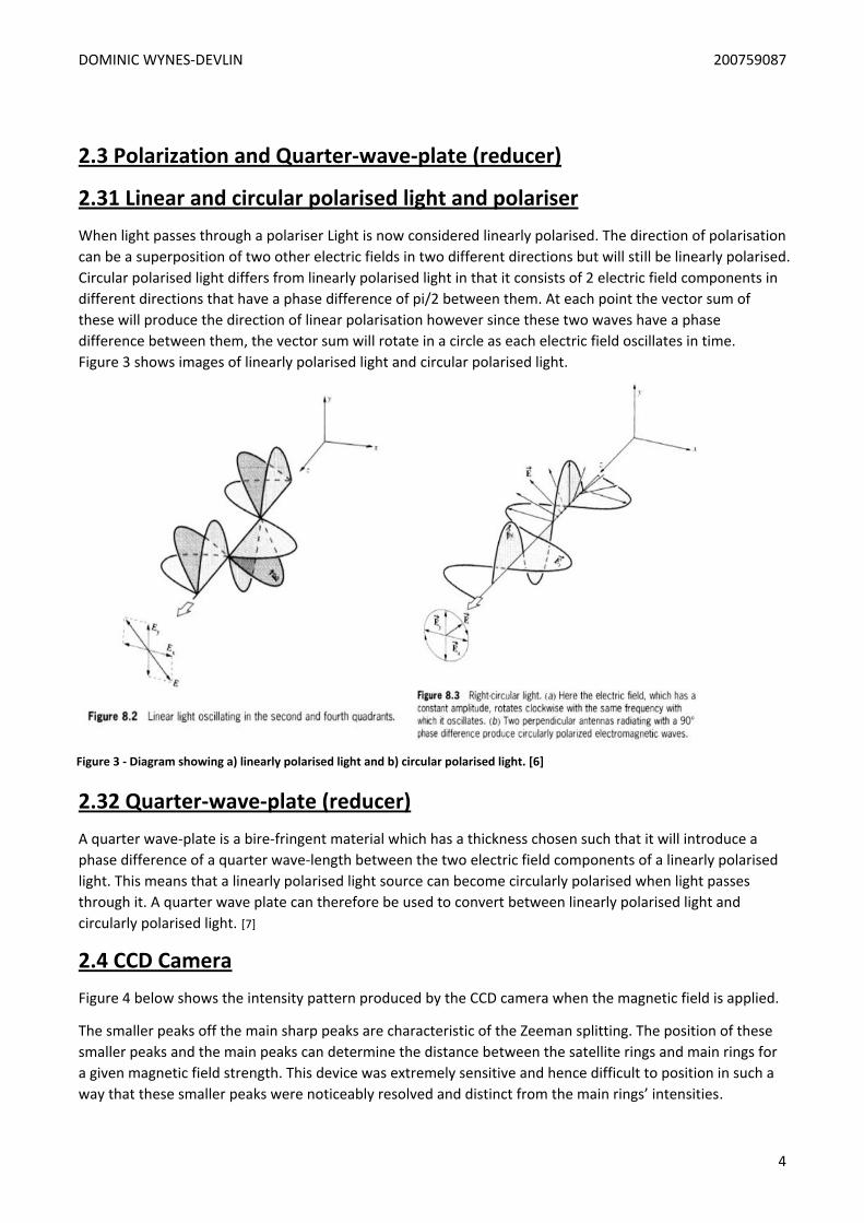
2.31 Linear and circular polarised light and polariser

When light passes through a polariser Light is now considered linearly polarised. The direction of polarisation

can be a superposition of two other electric fields in two different directions but will still be linearly polarised.

Circular polarised light differs from linearly polarised light in that it consists of 2 electric field components in

different directions that have a phase difference of pi/2 between them. At each point the vector sum of

these will produce the direction of linear polarisation however since these two waves have a phase

difference between them, the vector sum will rotate in a circle as each electric field oscillates in time.

Figure 3 shows images of linearly polarised light and circular polarised light.

2.32 Quarter-wave-plate (reducer)

A quarter wave-plate is a bire-fringent material which has a thickness chosen such that it will introduce a

phase difference of a quarter wave-length between the two electric field components of a linearly polarised

light. This means that a linearly polarised light source can become circularly polarised when light passes

through it. A quarter wave plate can therefore be used to convert between linearly polarised light and

circularly polarised light. [7]

2.4 CCD Camera

Figure 4 below shows the intensity pattern produced by the CCD camera when the magnetic field is applied.

The smaller peaks off the main sharp peaks are characteristic of the Zeeman splitting. The position of these

smaller peaks and the main peaks can determine the distance between the satellite rings and main rings for

a given magnetic field strength. This device was extremely sensitive and hence difficult to position in such a

way that these smaller peaks were noticeably resolved and distinct from the main rings’ intensities.

Figure 3 - Diagram showing a) linearly polarised light and b) circular polarised light. [6]


5

Figure 4 – Intensity plot against distance in pixels for the light with the applied magnetic field. [8]

3. Observations of the Zeeman Effect

3.1 – Observed effect of applied magnetic field

When the magnetic field is applied in the transverse case the interference pattern produces main rings and

satellite rings. Where as, in the case of the longitudinal position no main rings are present since the pi

components are not present when the magnetic field is parallel to horizontal track. We can deduce that

main rings are therefore the pi components and the sigma components are the satellite rings.

3.2 – Varying the voltage through electromagnet

Increasing the voltage (hence the current) of the electromagnet results in the distance between the satellite

rings increasing. This causes the higher satellite rings of the lower order to become closer to the lower

satellite ring of the next higher order satellite ring and as such make some of the rings appear more closely

packed where as others appear greater spread out.

Figure 5 – Interference rings produced for: a) no applied magnetic field, an applied magnetic field in b) the transverse

position, c) the longitudinal position.

Figure 6 – Interference rings produced when applied voltage has increase for a) the transverse position, b) the longitudinal position.


6

3.3 – Introducing Polarizer and Quarter-Wave plate

3.31 – Adding Polariser

When the polariser is introduced into the transverse setup, both the main rings and satellite rings appear

when the polariser is set at 0 degrees to the vertical axis; where as, when the polariser is turned to 90

degrees only the satellite rings are visible. This is because the main ring is linearly polarised in the vertical

direction and so when the polariser is at 90 degrees the light cannot pass through it. This is because the pi

components of the main rings are linearly polarised, where as the satellite rings are the sigma components

and are circularly polarised hence they can still pass through the polariser. These observations are shown in

figure 7 below.

3.32 – Polariser and Quarter-wave-plate

When the quarter wave-plate is introduced in the longitudinal setup, circularly –polarised light becomes

linearly polarised. Since no pi components are present in the longitudinal position only the satellite rings can

be observed. When the polariser is at 0 degrees both satellite-rings can be observed. However when the

polariser is at 45 degrees only the outer satellite ring is observed, whereas when the polariser is changed to

-45 degrees (45 degrees anti-clockwise) only the inner satellite ring is observed. We can deduce from figure

1b) that the sigma plus components are anti-clockwise circularly polarised (ACCP) and the sigma minus are

clockwise circularly polarised (CCP) such that when the polariser is at 45 degrees then only the CCP light can

pass through and hence the outer satellite ring is visible and is the sigma plus component. The sigma

minus component must therefore be the inner satellite ring.

Figure 7 - Image of Interference rings for transverse position with a) no polariser, the polariser is at b) 0 degrees to the vertical axis,

c) at 90 degrees to the vertical axis.

Figure 8 - Image of Interference rings with polariser and quarter wave-plate for the polariser at a) 0 degrees to the vertical

axis, b) 45 degrees to vertical axis , c) -45 degrees to the vertical axis.


7

4. Calibration of Electro-magnet

The Electro-magnet is calibrated to determine a relationship between the applied current supplied to the

Electromagnet and the magnetic field strength between the two electromagnets. The magnetic field

strength between the electromagnets is measured using a Gauss meter which has a sensitivity of ± 1mT

(0.001T). The magnetic field strength was measured for varying current values from 5.05 to 8.88 A with

intervals of approximately 0.5 A. This data (shown in Table 1 below) is then used to plot the Calibration curve

for the applied current – I against the Magnetic field strength- B; shown in figure 8 below.

Table 1: Data for the applied current – I, magnetic field strength – B of the Electromagnets for current values range from

5.05- 8.88 A.

Figure 8 – Calibration curve of the applied voltage against the magnetic field strength of the electro-magnet.

V (V) B (T)

5.05 ± 0.01 5.51 ± 0.01 6.02 ± 0.01 6.51 ± 0.01 6.98 ± 0.01 7.51 ± 0.01 7.97 ± 0.01 8.51 ± 0.01 8.88 ± 0.01

0.278 ± 0.001 0.295 ± 0.001 0.315 ± 0.001 0.330 ± 0.001 0.343 ± 0.001 0.355 ± 0.001 0.364 ± 0.001 0.374 ± 0.001 0.374 ± 0.001

Voltage - V (V)


8

5. Determining the value of the Bohr magneton

The magnetic field values were determined by taking the voltages from the power supply and using the

calibration curve to find the magnetic field associated with these values. Table 2. Shows the magnetic field

values and the corresponding energy difference values. The Energy difference Ediff is then plotted as against

the magnetic field strength. This is shown in figure …

The energy difference Ediff can be related to the angular separation from the centre to the main ring−𝛼.

𝑬𝒅𝒊𝒇𝒇 = −𝜶 ∆𝜶

𝒏𝟐𝑬 (𝟐)

𝒅 = 𝑳𝜶 (𝟒)

Which also implies that:

𝜟𝒅 = 𝒍 𝜟𝜶 (𝟓)

We arrive at the final equation:

𝑬𝒅𝒊𝒇𝒇 =−𝒅∆𝒅

𝒏𝟐𝑳𝟐𝑬 (𝟔)

Where L (=150mm) is the distance between the imaging lens and the CCD camera lens, n is the refractive

index of the etalon (=1.457), d is the distance from the centre to the main ring, and ∆𝑑 is the average

distance between the main ring and satellite rings for a given magnetic field strength.

The Energy E can be determined from the equation 7:

𝑬 =𝒉𝒄

𝝀 (𝟕)

Where hc ≈1240 eV nm, and 𝜆 = 644 𝑛𝑚. Giving a value of E = 3.08075 E-24(J)

Table 2: Data for magnetic field strength – B and Energy difference Ediff.

B (T) Ediff (10-24 J)

0.294 ± 0.001 0.315 ± 0.001 0.330 ± 0.001 0.350 ± 0.001 0.365 ± 0.001

6.25 ± 0.01 6.40 ± 0.01 6.40 ± 0.01 6.55 ± 0.01 6.71 ± 0.01


9

Figure 9- Graph of Ediff against the B.

Since the Bohr-magneton is related to Ediff and B by:

𝑬𝒅𝒊𝒇𝒇 = 𝝁𝑩𝑩

The value can be determine from the slope of the graph of Ediff against B in figure…. This gives the value of

the Bohr magneton to be 𝝁𝑩 = (6.1 ± 0.9)E-24 (J/T). This gives a percentage error from the true value of 34.2%

which means that the experiment cannot be considered accurate. However the fractional error can be

considered reasonably precise with a percentage error of ≈ 15%

6. Discussions and Conclusion

The experimental value for the Bohr Magneton has been determined to be 𝝁𝑩 = (6.1 ± 0.9)E-24 (J/T).

Furthermore, the apparatus was correctly set up to observe the Zeeman splitting via the production of main

–rings and satellite rings in the interference pattern. The different components of the light (i.e. sigma+,

sigma- , and pi) were explained and related to their polarizations and the orientation of the applied magnetic

field.

Furthermore, it was observed that increasing the voltage in the Electromagnet resulted in a greater value for

the magnetic field strength and hence a resulted in a greater observed splitting in the energy levels (Zeeman

splitting). These observations agreed with our what we predicted to occur. A possible explanation for the

‘low’ value and hence large percentage error for the Bohr-magneton is that the applied magnetic field

strength measured by the gauss-meter was significantly lower than other experimental readings carried out

with different apparatus. The max value only reached 381mT in comparison to some readings between the

poles to be measured in other experiments to be around 500mT.


10

The initial readings for the magnetic field were much lower than the readings given in table (max B value of

250mT) which resulted in poorly observed Zeeman splitting which making the satellite rings blurry and not

sharp. The magnetic poles were adjusted so that they were closer to the lamp in-order to focus the magnetic

field lines. Upon this adjustment the values still did not change significantly. One possible explanation could

be that the coils might have become over-heated and therefore damaged due to the power supply being left

on for too long and as a result produces lower magnetic field readings than expected.

These factors meant that noticeable Zeeman splitting would only occur for large voltage/current values. If

the power supply was not capped at 9V then it might have been possible to observe more dramatic changes

in the energy difference and observe sharper distinctions between the satellite and main rings in the CCD

camera. However, this was not possible and as a result made it difficult to observe much change in the

splitting of the energy levels due to the weak magnetic field strength. This is evident in table 2, where the

second and third values for the Energy difference did not change at all for the increasing magnetic field

strength. This meant that resolving the positions of the satellite rings from the main rings was difficult to and

as such did not result in as large a differences in the positions.

One possible improvement could be to determine the initial main rings using the CCD and then applying the

magnetic field in the longitudinal configuration when the main rings are not present and determining these

positions with varying magnetic fields strengths using the CCD camera. A larger energy difference would

result in higher values for plotted points for the graph of Ediff against B and hence would have resulted in a

larger gradient value that was closer to the accepted Bohr-magneton value.

7. References

1. Hyperphysics.phy-astr.gsu.edu,. 'Vector Model Of Angular Momentum'. N.p., 2015. [Accessed 6 Dec. 2015.]

2. Haken, H, and H. C Wolf. The Physics Of Atoms And Quanta. Berlin: Springer-Verlag, 216 (1994), Print.

3. The Zeeman Effect, Lab Manual, University of Leeds, School of Physics and Astronomy, 117 (2015), Print

4. Hyperphysics.phy-astr.gsu.edu,. 'Hydrogen Schrodinger Equation'. N.p., 2015. [Accessed 6 Dec. 2015.]

5. Physics.nist.gov,. 'CODATA Value: Bohr Magneton'. N.P., (2015). [Accessed 6 Dec. 2015].

6. Hecht, Eugene. Optics. Reading, Mass.: Addison-Wesley, 333-334 (2002). Print.

7. Hyperphysics.phy-astr.gsu.edu,. 'Quarter-Wave Plate'. N.p., (2015). [Accessed 6 Dec. 2015.]

8. Zeeman Effect, Advanced Physics Laboratories, University of Michigan, Physics, 6(2006), available at:

http://instructor.physics.lsa.umich.edu/adv-labs/Zeeman/Zeeman.html [Accessed 6 December 2015]

http://instructor.physics.lsa.umich.edu/adv-labs/Zeeman/Zeeman.html

Formal Report Zeeman.docx

Documents

Transcript of Formal Report Zeeman.docx