Form Factors, Grey Bodies and Radiation … Factors...1 Form Factors, Grey Bodies and Radiation...

1

Form Factors, Grey Bodies and Radiation Conductances (Radks)

Presented by: Steven L. Rickman

NASA Technical Fellow for Passive Thermal NASA Engineering and Safety Center

Thermal and Fluids Analysis Workshop 2012

Pasadena, California August 2012

NASA Photo: ISS027E036658

Introduction

2

With today's analysis tools, large, complex thermal radiation problems are easily solved; But, as with any analytical tool, lack of an understanding of the fundamental equations and technique limitations may leave you with the wrong answer; Whether you are a new engineer or a seasoned veteran, an understanding of the techniques employed by these powerful analysis tools is crucial.

Overview

3

This lesson explores thermal radiation analysis techniques for form factors, grey body factors and Radks.

Scope of this Lesson

4

The Radk and its role in thermal analysis; Form factor calculation techniques; Grey body factor calculation techniques; Radiation Conductance (Radk).

Lesson Roadmap

5

Fundamentals What is a Radk?

Form Factors

Double Area Summation

Nusselt Sphere

Form Factors Using Monte Carlo Ray

Tracing

Form Factor Reciprocity and Combinations

Grey Body Factors

Gebhart's Method

Calculating Grey Body Factors Using

Monte Carlo Ray Tracing

The "World's Worst Dart Player"

Statistical Error

Imperfect Form Factor Sums

The Fence Problem

Turning the Grey Body Factor into a

Radk

Application in Analysis

Exact Solutions

Crossed-String Method

Approximating F

6

Fundamentals

The Blackbody

7

A blackbody is the perfect absorber and emitter of radiant energy; The Stefan-Boltzmann law shows that energy radiated from a blackbody is a function only of its absolute temperature, T: where = 5.67 10-8 W/m2 K4.

The Grey Body

8

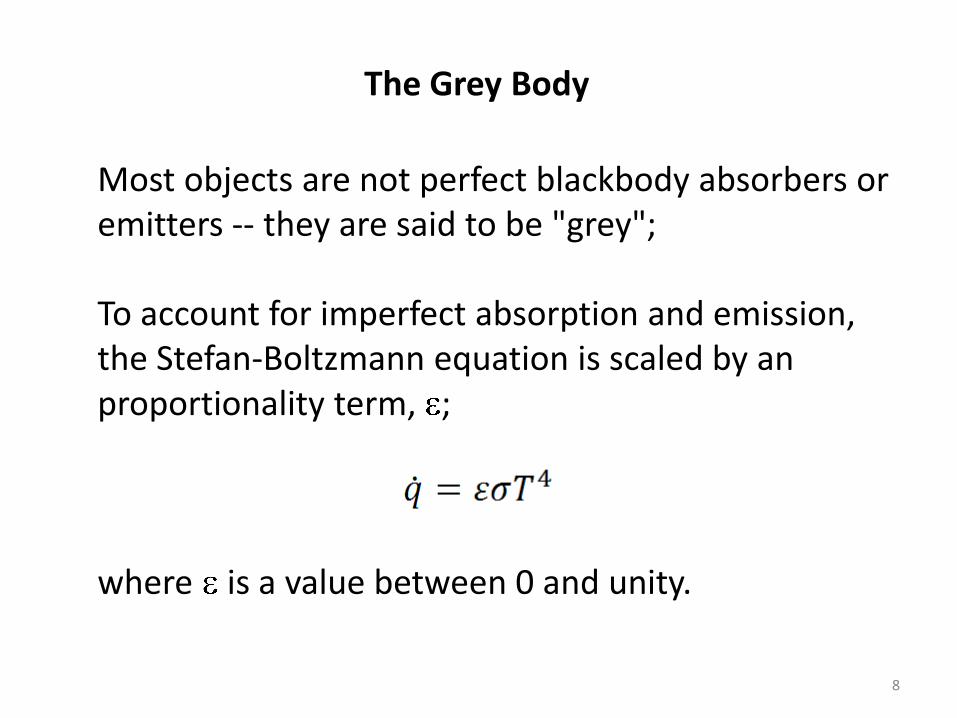
Most objects are not perfect blackbody absorbers or emitters -- they are said to be "grey"; To account for imperfect absorption and emission, the Stefan-Boltzmann equation is scaled by an proportionality term, ; where is a value between 0 and unity.

Conservation of Energy

9

Conservation of energy tells us that the fraction of energy absorbed by a surface, plus the energy reflected, plus the energy transmitted, must equal the energy incident on that unity: For an opaque surface, = 0 and the equation simplifies to:

1=++

1=+

Conservation of Energy

10

If we limit our discussion of absorption and emission to the same portion of the spectrum (or, more precisely, to a given wavelength, ), we can say: For the purpose of our discussion, we're going to use for, both, absorption and emission in the infrared

spectrum.

Kirchhoff's Law

11

This says, for a given wavelength, , an object's ability to absorb radiant energy is equal to its ability to radiate energy; Consider an object with surface area, A, and emittance, at temperature, T1, introduced into an oven at T2.

T2

T1

A

Kirchhoff's Law

12

At steady state, there is no net heat transfer so the object warms until is reaches T2; When the object reaches T2, the amount of energy per unit time being absorbed is equal to that being radiated.

T2

T2

A

Kirchhoff's Law

13

The only way for this to be true is for:

T2

T2

A

Emittance

14

For thermal radiation, we generally consider the range of > 4000 nm to be in the infrared range (Ref. 1); We use to describe absorption and emission of radiation in this wavelength range.

Planck Blackbody Curve for 300 K

Diffuse and Specular Reflection

15

We saw previously that when energy strikes a surface, it may be absorbed, transmitted, or reflected; For our discussion, we're going to consider only opaque surfaces; In this case, transmitted radiation is zero.

Incoming Energy

Transmitted Energy

Reflected Energy

Absorbed Energy


16

Reflection may occur in a number of ways: Diffuse -- energy striking a surface is scattered in all directions; Specular -- the energy angle of incidence is equal to the angle of reflection in the pure case; Mixed -- a combination of both, diffuse and specular modes.


17

Diffuse -- energy striking a surface is scattered in all directions.


18

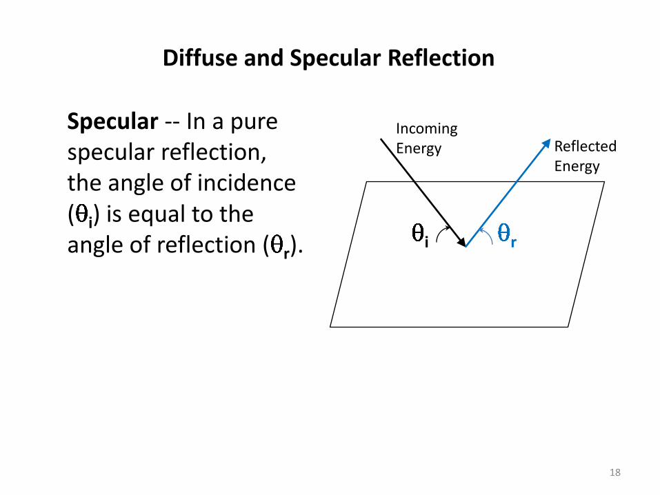
Specular -- In a pure specular reflection, the angle of incidence ( i) is equal to the angle of reflection ( r). i r

Incoming Energy Reflected

Energy


19

Mixed-- A combination of, both, diffuse and specular reflections; In this case, we consider a specular fraction -- the fraction of the total reflected energy that is reflected specularly.

Incoming Energy

Reflected Energy (Diffuse)

Reflected Energy (Specular)

Real Surfaces

20

Reflection from real surfaces is often more complex than the pure diffuse or specular case; Bidirectional reflectance distribution function (BRDF) (Adapted from Ref. 2).

Angle from Specular In Incidence Plane, deg Wavelength = 10.63 m

S13-GLO Painted Aluminum

BR

DF,

1/s

r

i = 5°

i = 37°

i = 53°

i = 66°

i = 78°

21

What is a Radk and What is its Role in Heat Transfer?

Conduction, Convection and Radiation

22

Heat is transferred by three distinct modes: Conduction; Convection; Radiation.

The Thermal Network

23

The goal of thermal analysis is to represent, accurately, the physics of heat transfer phenomena; Nodes represent objects with mass (diffusion), objects that can reasonably be modeled as massless (arithmetic), and substantial heat sinks (boundary); Conductors represent heat flow paths.

The Thermal Network

24

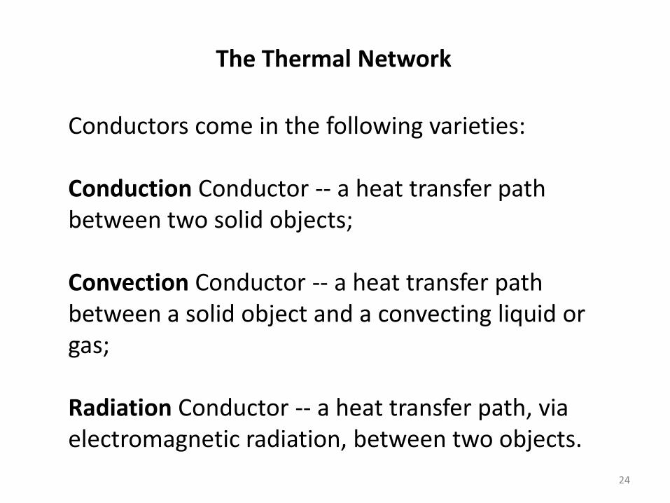
Conductors come in the following varieties: Conduction Conductor -- a heat transfer path between two solid objects; Convection Conductor -- a heat transfer path between a solid object and a convecting liquid or gas; Radiation Conductor -- a heat transfer path, via electromagnetic radiation, between two objects.

The Thermal Network

25

Heat transfer via conduction and convection is proportional to T: But, heat transfer via radiation takes this form:

The Thermal Network

26

Differential equation solvers for thermal analysis solve linear differential equations; The introduction of radiation into thermal networks adds non-linearity to the problem; But, the radiation portion of the thermal network can be linearized to make solution as part of the overall network possible.

The Thermal Network (Ref. 3)

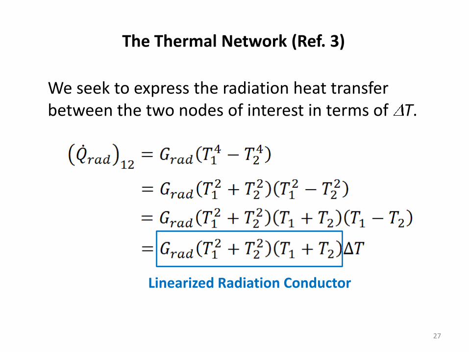
27

We seek to express the radiation heat transfer between the two nodes of interest in terms of T.

Linearized Radiation Conductor

The Thermal Network

28

But what about the Grad term? This is the radiation conductor, or, Radk for short; Developing the Radk, via form factors and grey body factors, will be the focus of the remainder of this lesson.

The Thermal Network

29

Consider the following geometry:

1

2

3

4 (Space)

The Thermal Network

30

Considering only conduction between the objects: 1 and 2 can exchange energy; 2 and 3 can exchange energy.

When we add radiation: 1 and 2 can exchange energy; 1 and 3 can exchange energy; 1 and 4 can exchange energy; 2 and 3 can exchange energy; 2 and 4 can exchange energy; 3 and 4 can exchange energy.

The Thermal Network

31

The thermal network looks like this:

32

Form Factors

The Form Factor

33

A form factor (a.k.a. shape factor, configuration factor, view factor) describes how well one object can "see" another object; The form factor may take on a value from zero to unity.

A form "factometer" was used in conjunction with a physical model to determine key form factors for radiation analysis; the technique used a partial spherical mirror and the projection of the reflected image of a target surface on the unit circle; With modern computers, however, calculating form factors is now an analytical pursuit.

The Form Factor

34

Exact Solutions

35

Throughout this lesson, we'll be exploring techniques for approximating the form factor between two surfaces; There are a limited number of geometries for which exact solutions exist; Having an exact solution available for comparison will help us show the benefit of the approximate methods.

Exact Solutions

36

We'll be using the geometry of parallel unit plates with unit separation throughout this lesson; Let's take a look at the exact solution for this geometry. For convenience, we define: X = a/c and Y = b/c

A1

A2

Exact Solutions (Ref. 4)

37

An exact solution is possible through a technique called contour integration:

A1

A2

Exact Solutions

38

For unit plates with unit separation: X = Y = 1 and the exact solution for FF12 becomes: FF12 = 0.2

A1

A2

The Form Factor

39

Form factors may be calculated using a variety of techniques including: Double area summation; Nusselt Sphere technique; Crossed-String method; Monte Carlo ray tracing; Contour integration; Hemi-cube.

We'll examine the highlighted techniques in detail.

40

The Double Area Summation Method

Double Area Summation

41

Consider, again, the integral defining the form factor: We see that finite area approximations may be made and summations may be substituted for the integrals:

Double Area Summation Example

42

Consider two parallel unit plates separated by one unit; We seek the form factor between surfaces a and b. We'll examine a number of solutions.

a

b


43

First, consider the case where each surface consists of one element (n = 1, m = 1); The angles ( a and b) between the line connecting the element centers and the surface normal is 0°; The distance (rab) between element center is 1.

b

a

rab

a

b


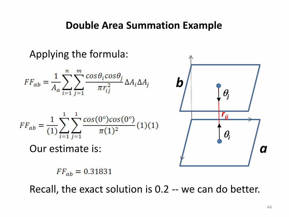
44

Applying the formula: Our estimate is: Recall, the exact solution is 0.2 -- we can do better.

j

i

rij

a

b


45

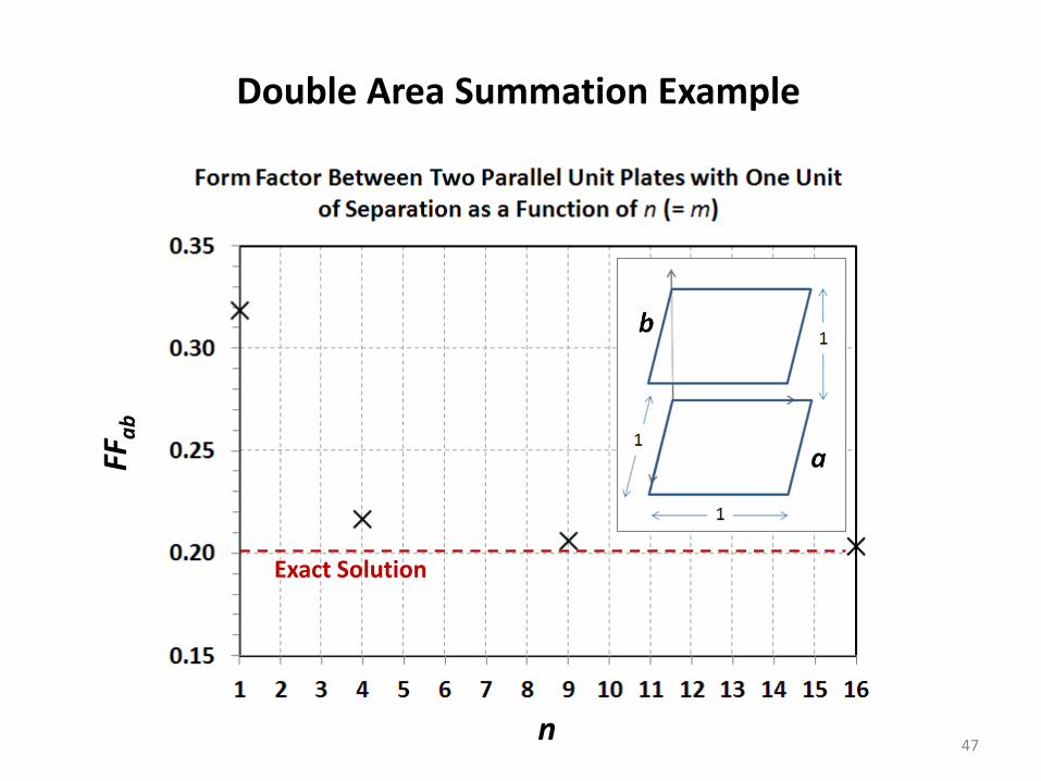
Let's subdivide each element into 4 subelements (n = 4, m = 4); The same calculation is performed for each subelement on the other surface; A total of 16 calculations is required.

a

b


46

The subelement to subelement calculations are :


47 n

FFa

b

Exact Solution

48

The Nusselt Sphere Method

Nusselt Sphere

49

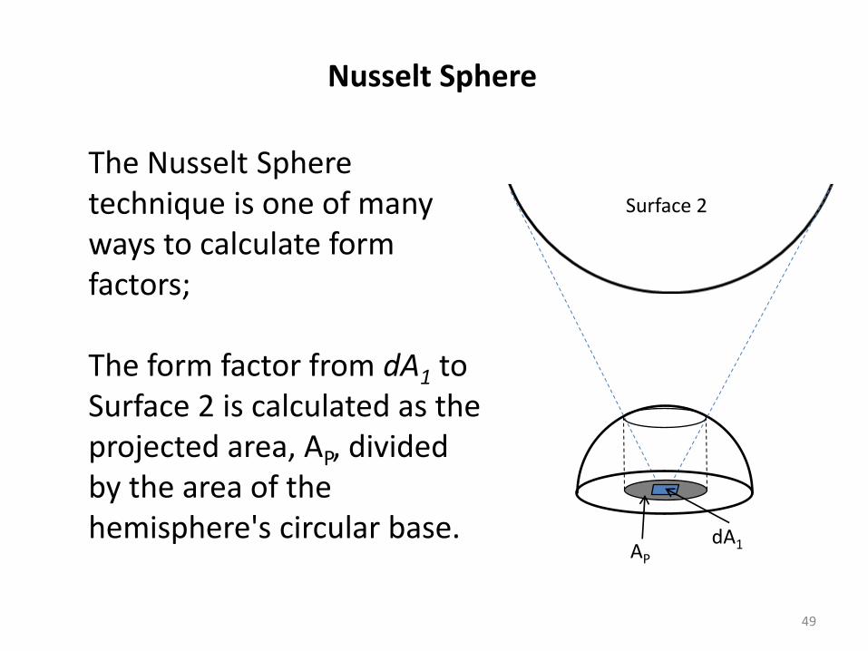
The Nusselt Sphere technique is one of many ways to calculate form factors; The form factor from dA1 to Surface 2 is calculated as the projected area, AP, divided by the area of the hemisphere's circular base.

Surface 2

dA1 AP

Nusselt Sphere

50

Let's use the Nusselt Sphere technique for calculating the form factor to the planet from an orbiting plate, at altitude h above the planet, whose surface normal faces the nadir direction.

Planet

dA1

re

AP

h

re

Nusselt Sphere

51

Planet

dA1

re

AP

h

re

re

We see that we can construct a right triangle (in green) with a short side measuring re and a hypotenuse measuring re+h; We define the angle by noting:

x

Nusselt Sphere

52

Planet

dA1

re

AP

h

re

re

Similarly, we can construct a right triangle (in red) with a hypotenuse measuring unity and the angle , already defined; We define the distance x by noting: r = 1

Nusselt Sphere

53

Planet

dA1

re

AP

h

re

re

Projecting x down to the base, we see that the ratio of the projected circular area to the total area of the base is: r = 1

x

54

The Crossed-String Method

Crossed-String Method (Ref. 5)

55

The Crossed-String method may be used on two dimensional geometries of infinite extent; The general formula for calculating a form factor between two surfaces is:


56

Consider the following two-dimensional geometry of infinite extent; We seek the form factor between surface 1 and surface 2.

Surface 2


57

Let's define our string lengths: L1 = 1.732 in L2 = 1.5 in L3 = 1.866 in L4 = 1.0 in L5 = 1.803 in L6 = 2.394 in

Surface 2


58

Solving...

Surface 2

59

The Monte Carlo Ray Tracing Method

Monte Carlo Methods

60

A Monte Carlo method uses random numbers to perform an integration; How can a random number can be used to accomplish such a feat? Furthermore, how can we get usable answers from anything involving random numbers? Let's start with an example.

Example -- The "World's Worst Dart Player"

61

To see how random numbers can be applied in integration, let's consider the challenge of approximating ; We'll establish a thought experiment, establish some equations to help us conduct this experiment, and then use random numbers to help us achieve our goal.


62

Suppose you encounter the World's Worst Dart Player...


63

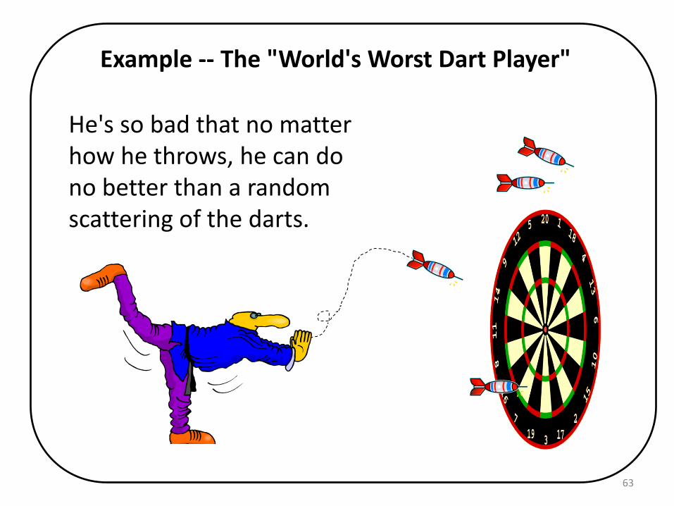
He's so bad that no matter how he throws, he can do no better than a random scattering of the darts.


64

So, to make the game fair, you decide to build a very large, circular dart board -- one that just fits onto a square wall; Our dart player may be the world's worst but he can certainly hit somewhere on the square wall!


65

Let's put some dimensions on our wall and dartboard -- represented here by a square and circle, respectively.

s

s

s/2


66

The area of the square is given by: And the area of the circle is, simply:

s

s

s/2

As = s2

Ac = s2/4


67

If all of our dart thrower's darts must land somewhere inside the square, the chances that a dart will land inside the circle will depend on the relative areas of the circle and the square.

s

s

s/2


68

In other words, for a large total number of darts, nt , we have: where nc is the number of darts that land inside the circle.


69

But, we have expressions for areas Ac and As: or... This gives us a framework for our numerical experiment.


70

Let's throw our first dart; If it lands inside the circle, our estimate of for nt = 1 is: Not bad for one dart.

4 (1/1) = 4


71

But since it's a random dart, it could have just as easily landed outside the dartboard; Our estimate becomes: Not so good.

4 (0/1) = 0


72

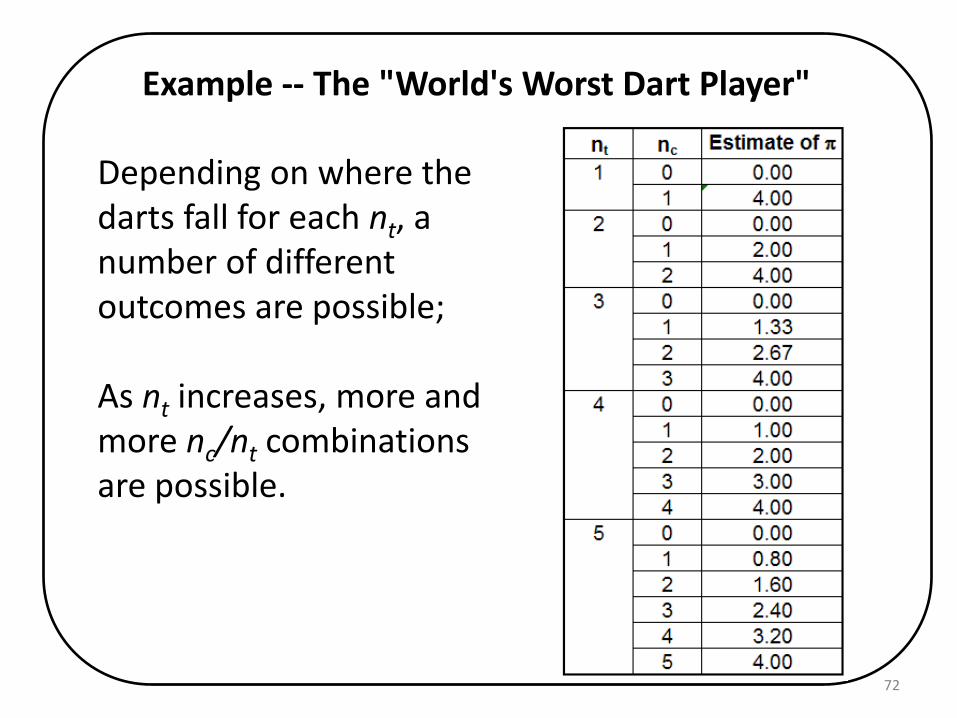
Depending on where the darts fall for each nt, a number of different outcomes are possible; As nt increases, more and more nc/nt combinations are possible.


73

This suggests that our ability to approximate accurately increases with the total number of darts thrown; Also, as nt increases, the addition of a single dart has less of an effect on the approximation of ; So, instead of simply throwing only a few darts, let's see what happens when we throw thousands of darts.


74

Total Number of Darts Thrown, nt

Esti

mat

e o

f

Predicted by Monte Carlo


75

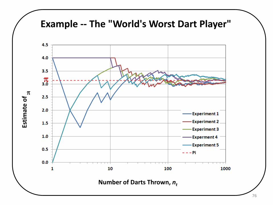
For this example our estimate of can vary dramatically for only a small number of darts; But, eventually, with enough darts, we get an excellent approximation of .


76

Number of Darts Thrown, nt

Esti

mat

e o

f

Calculating Form Factors Using the Monte Carlo Method

77

To calculate a form factor, we'd like our Monte Carlo simulation to represent the view from one surface over the region that surface can "see"; For example, a flat plate surface can "see" an entire hemisphere.


78

Our integration scheme will need to sample from the entire plate area (u, v), and all angles ( ,

); In this case, four random numbers are needed for each ray.


79

Consider the following geometry -- all surfaces are opaque.

1

2

3 4


80

Let's shoot 1000 rays from Surface 1; 200 rays hit Surface 2; 150 rays hit Surface 3; 80 rays hit Surface 4; The rest escape to Space.


81

The form factor between Surface 1 and the others is: FF12 = 200/1000 = 0.200 FF13 = 150/1000=0.150 FF14 = 80/1000 = 0.080 FF1SPACE = 570/1000 = 0.570


82

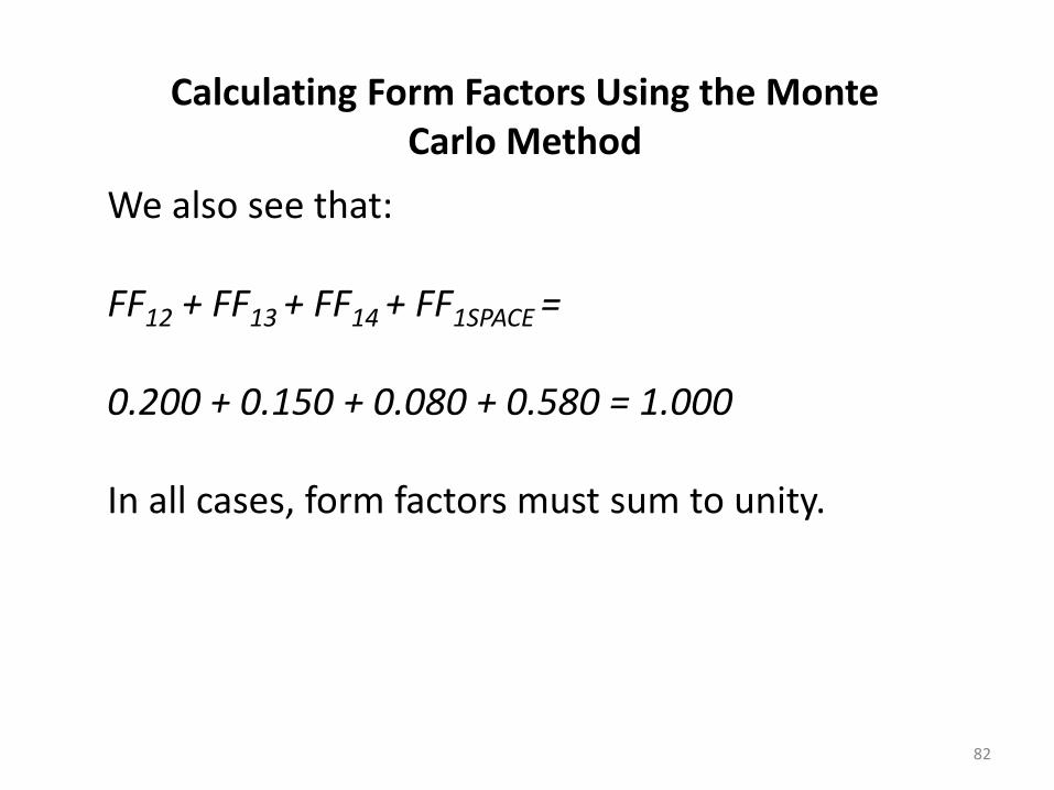
We also see that: FF12 + FF13 + FF14 + FF1SPACE = 0.200 + 0.150 + 0.080 + 0.580 = 1.000 In all cases, form factors must sum to unity.

Sample Problem

83

Consider two parallel unit plates separated by one unit; We'll apply the Monte Carlo method to calculate the form factor between these two surfaces.

1 m

1 m

Screen shot from RadCad® by Cullimore and Ring Technologies, Inc

Sample Problem

84

20 rays

220 rays

420 rays

720 rays


Sample Problem

85

The solution improves as the number of rays shot increases:


Statistical Error (Ref. 6)

86

If we are estimating a value generated by sampling a random distribution, we cannot be 100% certain of a bounding value unless we say that its value lies somewhere between - and + ; So if we're to generate meaningful answers using random variables, we'll need to be more realistic about the bounds; We can do this by specifying a confidence interval.


87

The Normal or Gaussian Distribution is given by: where...

is the mean value, and; is the standard deviation.


88

We will also consider the Cumulative Density Function (CDF): The CDF tells us the probability of a random variable falling in the interval (- , x);


89

We want to know the probability of a random variable falling in the interval ( -N , +N ): where N is the number of standard deviations ( ) from the mean value ( ).

Statistical Error

90

For example, for one standard deviation, N = 1, the probability of a random variable falling in the interval ( - , + ) is: In other words, we can say that a random variable has a 68.3% chance of being within one standard deviation of the mean -- or, to put it another way, we're 68.3% confident that the value lies somewhere within one standard deviation of the mean.

Statistical Error

91

If we want to establish an answer with 90% confidence, we would need to find N for the following: This occurs for N = 1.645.

Statistical Error

92

=1

90% Confidence

Interval

+1.6

45

-1.6

45

P(x

)


93

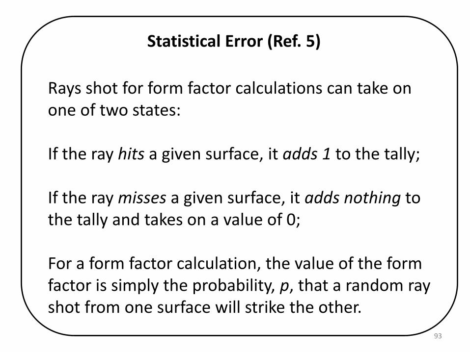
Rays shot for form factor calculations can take on one of two states: If the ray hits a given surface, it adds 1 to the tally; If the ray misses a given surface, it adds nothing to the tally and takes on a value of 0; For a form factor calculation, the value of the form factor is simply the probability, p, that a random ray shot from one surface will strike the other.


94

With only two possible states, we see this is a discrete distribution; To calculate the mean, of a discrete distribution, we use: where... xj is the value of an event, and; f(xj) is the probability of the event happening.


95

For a discrete distribution, the variance, 2, is: Note that j = 2 since x can take on a value of 0 or 1; But variance can be applied to, both, of a sample, s2, or of the mean, 2.


96

Form factor error estimation strategy we assume: The variance of a sample, s2, is approximately equal to the variance of the distribution: The variance of the distribution of means, m

2, calculated from n samples, is estimated by using the variance of the sample population:


97

If the mean value, is simply the probability, p, of the ray striking the other surface, then the probability of missing the surface is (1-p) and the variance becomes:


98

What we really seek is a variance of the means, m2:

For a 90% confidence interval, our estimate of our error:


99

When FF is high, (1-FF)/FF is low and n doesn't have to be large to achieve low error; When FF is low, (1-FF)/FF is high and n must be large, relatively speaking, to lower the error.

Statistical Error

100

How does that change the number of rays (n1/2) we have to shoot if we wish to halve the error? The number of rays required quadruples: n1/2 = 4n


101

For 90% confidence, the relationship between form factor magnitude, number of rays shot and the associated statistical error is:

Number of Rays

Form

Fac

tor

Mag

nit

ud

e

% Error

102

Form Factor Reciprocity and Combinations

Reciprocity

103

For two nodes i and j, we observe the following relationship: This is called reciprocity; We can use this to solve for unknown form factors in our geometry.

Form Factor Combinations (Ref. 3)

104

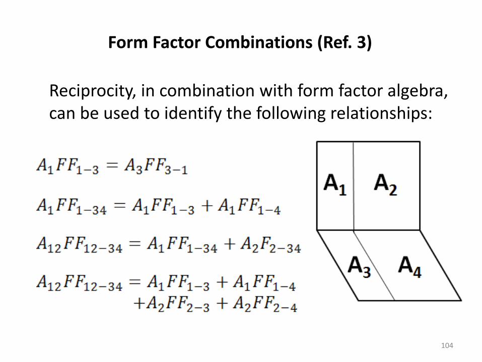
Reciprocity, in combination with form factor algebra, can be used to identify the following relationships:

Form Factor Combinations

105

Let's look at the form factor relationships for a cube:

1 m

1 m

1

2

3 4 5

6

Form Factor Combinations

106

We see that: But we see symmetry in this cube geometry so we conclude that: We'll use this result in an example problem later.

107

Grey Body Factors

Difference Between a Form Factor and Grey Body Factor

108

A form factor describes how well one object "sees" another object via direct view; In other words, a form factor quantifies the fraction of energy emitted from one surface that arrives at another surface directly; A grey body factor quantifies the fraction of energy leaving one surface that is absorbed another surface through all possible paths.

The Mirror Maze Analogy

109

Consider two friends, A and B situated at opposite ends of a maze comprised of mirrors; We ask, can the two friends see one another?

A

B


110

A cannot see B directly; We say that the form factor between A and B is zero;

A

B

X


111

But if the walls are mirrors, A can see B via reflection; In this case, the grey body factor between A and B is greater than zero.

A

B


112

Actually, there are many possible reflections that will allow A to see B; The grey body factor is the amount of energy that leaves A and is absorbed at B via all possible paths.

A

B

113

Gebhart's Method

114

Form factors are an intermediate product and, by themselves, have limited use; We really seek a means of determining how radiant energy is distributed in a thermal network; Form factors and surface emittances are inputs to Gebhart's method to calculate grey body factors which can readily be turned into Radks. This method works for diffuse interchange only.

Turning Form Factors Into Grey Body Factors

Gebhart's Method (from Ref. 9)

115

Define the Gebhart factor as: where i is one surface and j is another and Ai and Aj are surface areas of i and j, respectively.

Gebhart's Method (from Ref. 9)

116

For Ns objects, the general formula is: We also note for an object, i:

Gebhart's Method

117

For three objects that see only one another, we can establish the Bij values, holding i constant: By remembering that B11 + B12 + B13 = 1 and noting that reflectance, = (1- ), we can interpret each of these terms.

Gebhart's Method (Ref. 10)

118

Fraction leaving object 1... directly absorbed at j=1, 2, 3; reflecting off of 1 and is absorbed j=1, 2, 3; reflecting off of 2 and is absorbed at j=1, 2, 3; reflecting off of 3 and is absorbed at j=1, 2, 3; The B1j for j = 1, 2, 3 must sum to unity.

Gebhart's Method

119

1

2

1 2

Consider two infinite parallel plates with the specified properties; Given the infinite extent, we can say:

Gebhart's Method

120

Our expression for the Bij values becomes:

Gebhart's Method

121

Rearranging, yields the following: Grouping similar terms together:

Gebhart's Method

122

In matrix form, the system of equations becomes: Recall, for infinite parallel plates:

Gebhart's Method

123

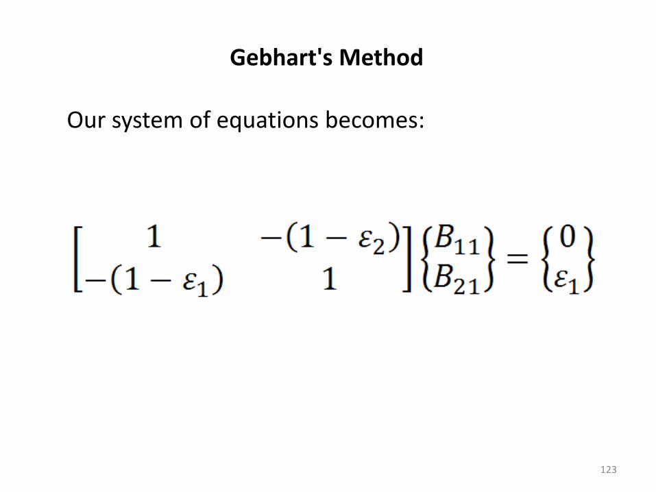
Our system of equations becomes:

Gebhart's Method

124

From the first equation, we see that: Substituting into the second equation yields: Finally, solving for B21:

Gebhart's Method

125

You may be more familiar with the infinite parallel plate solution that looks like this: is the ratio of the energy incident at surface 1 originating at surface 2 divided by the total radiation emitted at 2.

Gebhart's Method

126

But, remember, the B21 is the ratio of the energy absorbed at surface 1 originating as emission at surface 2 divided by the total radiation emitted at 2; The relationship between the two is:

127

We can establish an approximate value of F21 using

a simpler expression when the surface emittance values are relatively high. To do this, we can modify our expression for F21 by

multiplying the numerator and denominator by 1 2:

Approximating F21(Ref. 11)

128

This simplifies to: As 1 and 2 approach unity, the expression approaches 1 2.



129

Gebhart's Method Example

130

Consider an infinitely long enclosure with an equilateral triangular cross section; We wish to calculate the radiation interchange for the internal surfaces given:

1 = 2 = 3 = 0.05

1

2

3

1

2

3


131

Due to infinite extent and problem symmetry: FF11 = FF22 = FF33 = 0 FF12 = FF13 = 0.5 FF21 = FF23 = 0.5 FF31 = FF32 = 0.5 The FF sum for each node must equal unity. All FF to Space equal zero.

1

2

3

1

2

3


132

We apply our equation for Bij where Ns = 3: Our system of equations is:


133

Rearranging yields: In matrix form, the system of equations becomes:


134

Substituting values into the matrices: Solving for B11, B21 and B31:


135

We can use this example to explore the effect of imperfect form factor sums on energy conservation; Consider the same geometry but assume, this time, that whichever form factor approximation methodology we used left us with imperfect form factor sums: with other FFs inferred through symmetry.


136

In this instance, our form factors do not sum to unity: How does this affect energy conservation in the radiation network?


137

If we substitute the imperfect form factors into our system of equations, we get: Solving once again for B11, B21 and B31:


138

A check of energy conservation yields an imperfect summation: In this example, only about 83% of the thermal radiation interchange is represented by the network; This result cautions the analyst to ensure form factors sum to unity for each node.

139

Calculating Grey Body Factors Using the Monte Carlo Ray Tracing

Method

Calculating Grey Body Factors Using the Monte Carlo Method

140

We saw that Monte Carlo ray tracing can be used to calculate form factors; By extension, we can also use them to calculate grey body factors; Let's see how this works.


141

Consider the following geometry -- all surfaces are opaque.

1

2

3 4

1=0.3

2=0.4

3=0.6

4=0.8


142

A ray with unit energy is fired from a random location on Surface 1 and in a random direction; The rays hits Surface 2; What is the energy transfer?


143

Since the ray leaves Surface 1 with unit energy and hits a surface with an emittance of 0.4, we conclude that 40% of the energy is absorbed by Surface 2 and 60% is reflected.


144

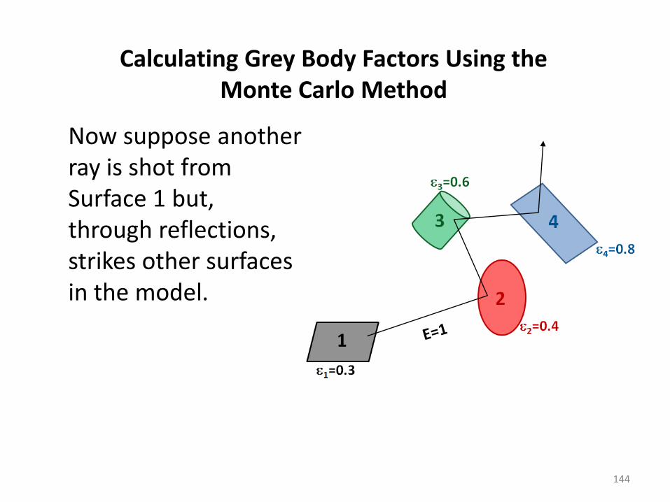
Now suppose another ray is shot from Surface 1 but, through reflections, strikes other surfaces in the model.


145

We can tally the energy deposited as the ray moves from reflection to reflection:


146

If many such rays are shot and a tally of energy deposition is maintained, we have an estimate of the fraction of energy leaving Surface 1 and arriving at Surface 2 via all possible paths.


147

A ray is traced until it leaves the geometry or the ray energy drops below a specified threshold; In the latter case, once this occurs, a test is performed at the next ray-to-surface intersection to determine whether the ray is completely absorbed or completely reflected -- depending on the surface properties; This allows for energy conservation.


148

In an enclosure, rays may undergo many bounces before the ray energy drops below the threshold to terminate the ray.

Single Ray Traced in Enclosure with = 0.05


Grey Body Statistical Error (Refs. 6 and 8)

149

A conservative error estimate is formed using discrete distribution assumptions also applies to grey body factors -- 90% confidence interval shown:

Number of Rays

Gre

y B

od

y Fa

cto

r M

agn

itu

de

% Error

150

The Fence Problem

The Fence Problem

151

The Fence Problem arises when the Gebhart technique is used without giving proper consideration to nodal boundaries; Let's examine how the Gebhart and Monte Carlo techniques handle this type of situation.

Consider the following geometry in which a fence is established at the midpoint of the long base rectangle. All surface emittances, = 0.5.

The Fence Problem

152

1

2

100 Node 100 is a single node spanning the entire base rectangle


Under normal circumstances, Nodes 1 and 2 should have no radiation coupling to one another.

The Fence Problem

153

1

2

100 Node 100 is a single node spanning the entire base rectangle


The Fence Problem

154

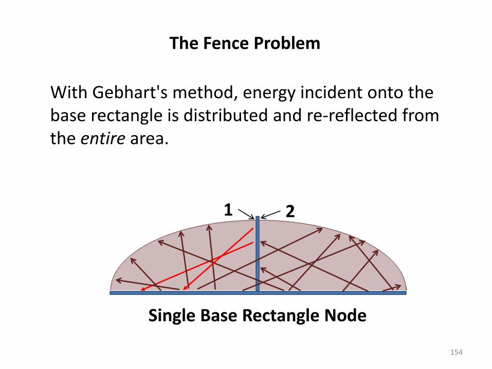
With Gebhart's method, energy incident onto the base rectangle is distributed and re-reflected from the entire area.

1 2

Single Base Rectangle Node

The Fence Problem

155

With a Monte Carlo (MC) approach, energy incident onto the base rectangle is re-reflected locally.

1 2

Single Base Rectangle Node (100)

Now consider the same geometry but with the base rectangle divided into two nodes:

The Fence Problem

156

1

2

100

101


The Fence Problem

157

Using Gebhart's method with a properly nodalized geometry, leakage of energy to the other side of the fence is prevented.

1 2

Two Base Rectangle Nodes 100 101

The Fence Problem

158

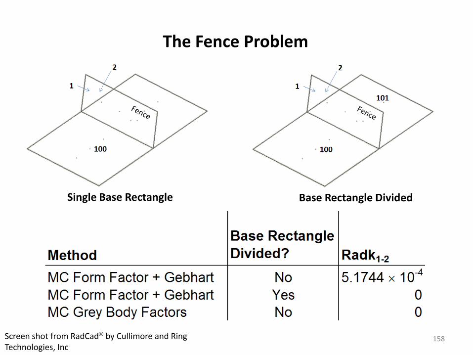
Single Base Rectangle Base Rectangle Divided


The Fence Problem

159

Diffuse reflection using Gebhart's method across the entire base rectangle results in a grey body factor between Nodes 1 and 2; When properly divided, the grey body factor between Nodes 1 and 2 is zero; Monte Carlo-generated grey body factors rely on reflection from the ray-surface intersection point and does not show the same nodalization sensitivity as does the Gebhart approach.

160

Turning the Grey Body Factor into a Radk

Turning a Grey Body Factor into a Radk

161

We've seen how to generate grey body factors using, either, form factors plus Gebhart's method or by direct generation of grey bodies using Monte Carlo methods; Now let's see how we can take the final step to turn the grey bodies into usable radiation conductances, or Radks.

Turning a Grey Body Factor into a Radk

162

The Radk (Grad)ij between two nodes i and j is given by: where i is the emittance of node i, Ai is the area of node i and Bij is the grey body factor from i to j. We also note:

Radk Screening

163

For configurations with a large quantity of nodes and/or highly reflective surfaces with view factors to one another, it is possible to generate an undesirably large quantity of Radks; Engineers must judge which couplings are significant; Radk dumps with different screening criteria may be used in thermal network models to determine the point of diminishing returns.

164

Application in Analysis

Example: Radiation in a Box

165

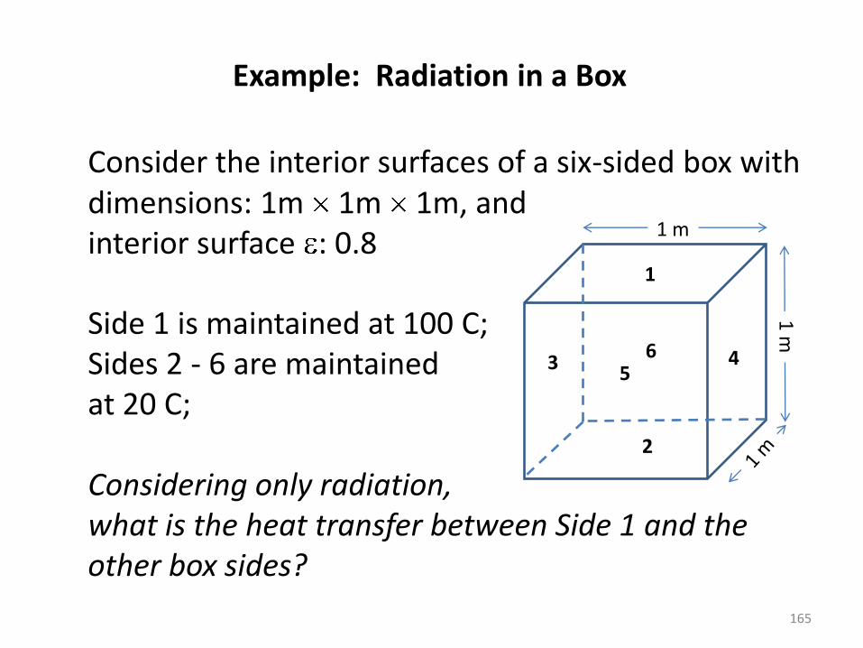
Consider the interior surfaces of a six-sided box with dimensions: 1m 1m 1m, and interior surface : 0.8 Side 1 is maintained at 100 C; Sides 2 - 6 are maintained at 20 C; Considering only radiation, what is the heat transfer between Side 1 and the other box sides?

1 m

1 m

1

2

3 4 5

6


166

The form factor solution for opposing parallel plates (Sides 1 and 2) yields an exact answer of 0.2; For the form factors to sum to unity, the form factor sum from Side 1 to the remaining Sides (3, 4, 5, 6) must be 0.8 (i.e., 1 - 0.2). By symmetry arguments:


167

If we wish to solve this using Gebhart's method, the system of equations for Side 1 will be:


168

Rearrange the equations into the form: Substituting known values, we have this system:

=


169

Our Bij values are: B11 = 0.038462 B12 = 0.192308 B13 = 0.192308 B14 = 0.192308 B15 = 0.192308 B16 = 0.192308 To obtain our Radks, we multiply by the area and the emittance of Side 1.


170

We can also use Gebhart's method using Monte Carlo-generated form factors -- we'll present this solution, as well, using 1,000,000 rays per node (and we'll assume reciprocity to find Fji given Fij); Finally, we'll form our Radks directly using Monte Carlo-generated grey bodies, again using 1,000,000 rays per node.


171

Comparing solutions...


172

The heat flow is... By similarity arguments, the heat transfer between Side 1 and all other sides is the same.

Concluding Remarks

173

A discussion of form factors, grey body factors and radiation conductors has been presented; Analytical formulations were shown for a variety of methodologies; Sample problems were provided to aid in understanding.

Acknowledgements

174

The author acknowledges the NESC Passive Thermal Technical Discipline Team for their valuable review and comments during the development of this lesson. Matt Garrison and Carol Mosier of GSFC are also acknowledged for their review of the draft lesson and their valuable comments.

References/Credits

1) Ungar, E. K., Slat Heater Boxes for Control of Thermal Environments in Thermal/Vacuum Testing, SAE 1999-01-2135, 1999. 2) Drolen, B., used with permission. 3) McMurchy, R., Thermal Network Modeling Handbook, 14690-H003-R0-00, NASA Contract 9-10435, January 1972. 4) http://www.me.utexas.edu/~Howell/sectionc/C-11.html 5) http://www.mhtl.uwaterloo.ca/courses/ece309/ lectures/pdffiles/summary_ch12.pdf.

175

References/Credits

6) TSS Theory Manual, Version 9.01, October 1999. 7) http://en.wikipedia.org/wiki/Normal_distribution 8) Thermal Radiation Analysis -- The Basics, Methodologies, and Use of Analysis Tools, Rickman, S.L. and Welch, M. 9) Gebhart Factor, http://en.wikipedia.org/wiki/Gebhart_factor

176

References/Credits

10) http://www.siggraph.org/education/materials/ HyperGraph/radiosity/overview_1.htm 11) Drolen, B., used with permission. Monte Carlo ray trace analyses and screen shots from RadCad® by Cullimore and Ring Technologies, Inc. Microsoft® clip art was used throughout this lesson.

177

For Additional Information

178

Closed-Form Form Factor Solutions - Schröder, P., Hanrahan, P., On the Form Factor Between Two Polygons, http://www.multires.caltech.edu/pubs/ffpaper.pdf Howell, J. R., A Catalog of Radiation Heat Transfer Configuration Factors, 3rd Edition, http://www.engr.uky.edu/rtl/Catalog/ Thermal Radiation Heat Transfer Siegel, R., Howell, J. R., Thermal Radiation Heat Transfer (Volumes I-III), NASA SP-164, 1968.

To Contact the Author

179

Address: Steven L. Rickman NASA Engineering and Safety Center (NESC) NASA - Lyndon B. Johnson Space Center 2101 NASA Parkway Mail Code: WE Houston, TX 77058 Phone: 281-483-8867 Email: [email protected]

Form Factors, Grey Bodies and Radiation … Factors...1 Form Factors, Grey Bodies and Radiation...

Documents

Transcript of Form Factors, Grey Bodies and Radiation … Factors...1 Form Factors, Grey Bodies and Radiation...