Forest Ecosystem Classification and Mapping for the … · forest ecosystem classification and...

Forest Ecosystem Classification and Mappingfor the Eden Comprehensive Regional

AssessmentA report undertaken for the NSW CRA/RFA Steering Committee

FOREST ECOSYSTEMCLASSIFICATION AND

MAPPING FOR THE EDENCOMPREHENSIVE

REGIONAL ASSESSMENT

DAVID KEITH AND MICHAEL BEDWARDBIODIVERSITY RESEARCH

AND SURVEY DIVISIONNSW NATIONAL PARKSAND WILDLIFE SERVICE

A report undertaken for the NSW CRA/RFA Steering Committeeproject number NE 18/EH

7 May 1998

Report Status

This report has been prepared as a working paper for the NSW CRA/RFA Steering Committee under thedirection of the Environment and Heritage Technical Committee. It is recognised that it may contain errors

that require correction but it is released to be consistent with the principle that information related to thecomprehensive regional assessment process in New South Wales will be made publicly available.

For more information and forinformation on access to data contactthe:Resource and Conservation Division, Department ofUrban Affairs and Planning

GPO Box 3927SYDNEY NSW 2001

Phone: (02) 9228 3166Fax: (02) 9228 4967

Forests Taskforce, Department of Prime Minister andCabinet

3-5 National CircuitBARTON ACT 2600

Phone: 1800 650 983Fax: (02) 6271 5511

© Crown copyright (May 1998)

This project has been jointly funded by the New SouthWales and Commonwealth Governments. The workundertaken within this project has been managed by thejoint NSW / Commonwealth CRA/RFA SteeringCommittee which includes representatives from the NSWand Commonwealth Governments and stakeholdergroups.

The project has been overseen and the methodology hasbeen developed through the Environment and HeritageTechnical Committee which includes representatives fromthe NSW and Commonwealth Governments andstakeholder groups.

DisclaimerWhile every reasonable effort has been made to ensurethat this document is correct at the time of printing, theState of New South Wales, its agents and employees, andthe Commonwealth of Australia, its agents andemployees, do not assume any responsibility and shallhave no liability, consequential or otherwise, of any kind,arising from the use of or reliance on any of theinformation contained in in this document.

CONTENTS

EXECUTIVE SUMMARY

1. INTRODUCTION 1

1.1 COMPREHENSIVE REGIONALASSESSMENT 1

1.2 APPROACH 1

1.3 STUDY AREA 2

2. METHODS 3

2.1 VEGETATION SAMPLING 32.1.1 Data Evaluation 32.1.2 Sample Stratification 52.1.3 Data Variables 5

2.2 VEGETATION DATA ANALYSIS 52.2.1 Classification Analyses 5

2.3 DESCRIPTIVE TECHNIQUES 6

2.4 SPATIAL DATA 7

2.5 SPATIAL MODELLING 8

2.6 MAP COMPILATION 9

2.7 MAP VALIDATION 92.7.1 Qualitative Checking 92.7.2 Accuracy Quantification 10

3. RESULTS AND DISCUSSION 11

3.1 FOREST ECOSYSTEM CLASSIFICATION11

3.2 FOREST ECOSYSTEM MAP 12

3.3 MAP VALIDATION 123.3.1 Qualitative Checking 123.3.2 Accuracy Quantification 12

4. REFERENCES 18

5. APPENDIX 20

5.1 DESCRIPTION OF FORESTECOSYSTEMS 20

FIGURES

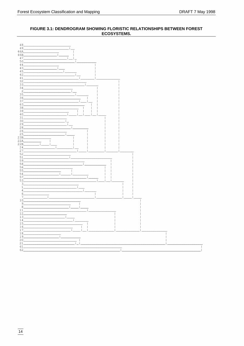
3.1: DENDROGRAM SHOWING FLORISTICRELATIONSHIPS BETWEEN FORESTECOSYSTEMS. 14

TABLES

2.1: VEGETATION DATA SETSEVALUATED 4

2.2: SAMPLE STRATIFICATION SCHEME 5

2.3: CONSENSUS RULES FOR SAMPLEASSIGNMENT 6

2.4: DEFINITIONS OF DIAGNOSTICSPECIES 7

2.5: SPATIAL DATA LAYERS USED INMODELLING 7

3.1: AREA OF FOREST ECOSYSTEMSERROR! BOOKM

1. EXECUTIVE SUMMARY

This report has been prepared for the jointCommonwealth/State Steering Committee whichoversees the comprehensive regional assessments(CRAs) of forests in New South Wales.

The CRAs provide the scientific basis on whichthe State and Commonwealth governments willsign regional forest agreements (RFAs) for themajor forests of New South Wales. Theseagreements will determine the future of the State’sforests, providing a balance between conservationand ecologically sustainable use of forestresources.

This report was undertaken to develop aclassification and map of forest ecosystems for theEden region, consistent with specifications of theJoint ANZECC/MCFFA National Forest PolicyStatement Implementation Sub-committee (JANIS1997). Forest ecosystems are the primarysurrogates for biodiversity used in CRAs.

The scope of this work, as approved by theEnvironment and Heritage Technical Committee,was to ‘refine the [Interim Forest Assessment]map, incorporating the best available past andproposed aerial photo-interpreted mapping,additional audited survey plot data and improvedterrain, substrate and climate variables.’

To achieve this end, forest ecosystemclassification in Eden followed an approachrecommended by the Forest Ecosystem WorkingGroup (1997) which had previously been appliedin the Interim Forest Assessment Process(RACAC 1996, Keith et al. 1995). The approachentailed: hierarchical multivariate classification offloristic data; definition of ecosystem units fromthe hierarchy based on their floristic, structural andenvironmental integrity; and mapping usingenvironmental relationships and remote sensing(Aerial Photography Interpretation) as a basis forspatial interpolation. Modification of the map usedin the Interim Forest Assessment (IFA) was alsorequired to accommodate new data and to extendthe analysis over an additional 140 000 hectares in

the north-west of the region (Numeralla-Wadbilliga).

Seventy-six forest ecosystems were classified andmapped in the Eden region, including 47 forestsdominated by eucalypts, six rainforests or scrubforests with rainforest affinities, 12 shrublands andheathlands, and three swamps. Four ecosystemswere estuarine wetlands associated with the hightide mark and a further four ecosystems wererestricted to estuaries below low tide mark (seagrass meadows) and consequently were excludedfrom the CRA. Comprehensive descriptions ofeach ecosystem are presented in this report.

Ecosystems were mapped using a hybrid decisiontree model/expert system that was developed andproofed iteratively. The model related theoccurrence of ecosystems to spatial patterns inmapped environmental variables (parent material,terrain and climate) and in the structure andcomposition of the tallest vegetation stratum asinterpreted from aerial photographs. The resultingmap of pre-1750 ecosystems was cut using a 1994Landsat coverage of extant native vegetation coverto derive extant distributions of forest ecosystems.An assessment of map accuracy using independentsample data indicated 92% accuracy within spatialneighbourhoods of 95 hectares. The forestecosystem map is available under licence from theNSW National Parks and Wildlife Service.

1

1. INTRODUCTION

1.1 COMPREHENSIVE REGIONALASSESSMENT

As part of the Regional Forest Agreement (RFA)process, a Comprehensive Regional Assessment(CRA) was carried out to evaluate the economic,social, cultural, environmental and heritage valuesof the Eden region. The CRA provided scientificinformation needed to develop a comprehensive,adequate and representative (CAR) forest reservesystem, the establishment of which is an agreedoutcome of RFAs and a commitment of theNational Forest Policy Statement (Commonwealthof Australia 1992). Studies carried out under theCRA are intended to refine the results ofpreliminary studies carried out as part of anInterim Forest Assessment Process (IFA).Regional Forest Agreements will also establish aregime of Ecologically Sustainable ForestManagement for all forest tenures in New SouthWales, as well as a framework for agreed socialand economic outcomes on forest use.

Components of CRAs involving environmentaland heritage values including biodiversity areoverseen in New South Wales by the Environmentand Heritage Technical Committee. Theconservation status of biodiversity will be assessedagainst conservation criteria at several agreedlevels including ecosystems, species, wildernessand old growth (JANIS 1997).

The conservation criteria followed in New SouthWales CRAs were defined in general terms byJANIS (1997). These criteria recognisebiodiversity as a highly complex system of livingthings incorporating variation at the genetic,species and ecosystem levels (Commonwealth ofAustralia 1995). Given the logistic difficulty ofsurveying and assessing representation of allelements of biodiversity, maps of speciesassemblages are widely recognised in conservationbiology as potential ‘surrogates’ or ‘coarse filters’

for biodiversity (Austin and Margules 1986, Noss1987).

JANIS (1997) identified ‘Forest Ecosystems’ asthe primary surrogate for biodiversity in CRAs.Forest Ecosystems were therefore used as a basisfor the assessments of biodiversity. For thedevelopment of a CAR reserve system in CRAs,JANIS (1997) established the following guidelinesfor representation of Forest Ecosystems inreserves:

■ 15% of the pre-1750 distribution of each ForestEcosystem, with flexibility considerationsapplied;

■ 60% of remaining extent of vulnerable ForestEcosystems; and

■ all remaining occurrences of rare andendangered Forest Ecosystems reserved orprotected by other means as far as practicable.

JANIS (1997) defined Forest Ecosystems andoffered advice for application of Forest Ecosystemmapping as a surrogate for biodiversity in CRAsas follows:

A Forest Ecosystem is ‘an indigenous ecosystemwith an overstorey of trees that are greater than20% canopy cover. These ecosystems shouldnormally be discriminated at a resolution requiringa map-standard scale of 1:100 000. Preferablythese units should be defined in terms of floristiccomposition in combination with substrate andposition within the landscape.’

The aim of this project was to prepare aclassification and map of forest ecosystems for theEden CRA region.

1.2 APPROACH

The scope of this project, as approved by theEnvironment and Heritage Technical Committee,was to ‘refine the [Interim Forest Assessment]map, incorporating the best available past andproposed aerial photo-interpreted mapping,

Forest Ecosystem Classification and Mapping DRAFT 7 May 1998

2

additional audited survey plot data and improvedterrain, substrate and climate variables.’

To achieve this end, forest ecosystemclassification in Eden followed an approachrecommended by the Forest Ecosystem WorkingGroup (1997) which had previously been appliedin the Interim Forest Assessment Process(RACAC 1996, Keith et al. 1995). The approachentailed: hierarchical multivariate classification offloristic data; definition of ecosystem units fromthe hierarchy based on their floristic, structural andenvironmental integrity; and mapping usingenvironmental relationships and remote sensing(Aerial Photography Interpretation) as a basis forspatial interpolation. The use of floristics,substrate and topographic position (as in JANIS1996) to guide definition of ecosystem units fromthe hierarchy was to constrain an otherwisearbitrary choice of the number of units in theecosystem classification to a scale of detailintended by the JANIS (1996) criteria.Modification of the IFA map was also required toaccommodate new data and to extend the analysisand mapping over an additional 140 000 hectaresin the north-west of the region (Numeralla-Wadbilliga).

1.3 STUDY AREA

The study area for the Eden ComprehensiveRegional Assessment is the Eden Native ForestManagement Area situated between latitudes 36°20’S and 37° 30’S and longitudes 149° 00’E and150° 05’E. The region is bounded by the coast inthe east, the Monaro Tableland in the west along aline from Nimmitabel to Bombala, the New SouthWales-Victorian state border in the south and aline stretching west from Bermagui in the north.

The region covers approximately 800 000 hectaresincluding areas of natural vegetation, dedicatedprimarily to timber production and conservation,and areas of cleared land used mainly foragriculture and plantation forestry. The climate,physiography and geology of the region isdescribed by Keith and Sanders (1990).

3

2. METHODS

2.1 VEGETATION SAMPLING

2.1.1 Data Evaluation

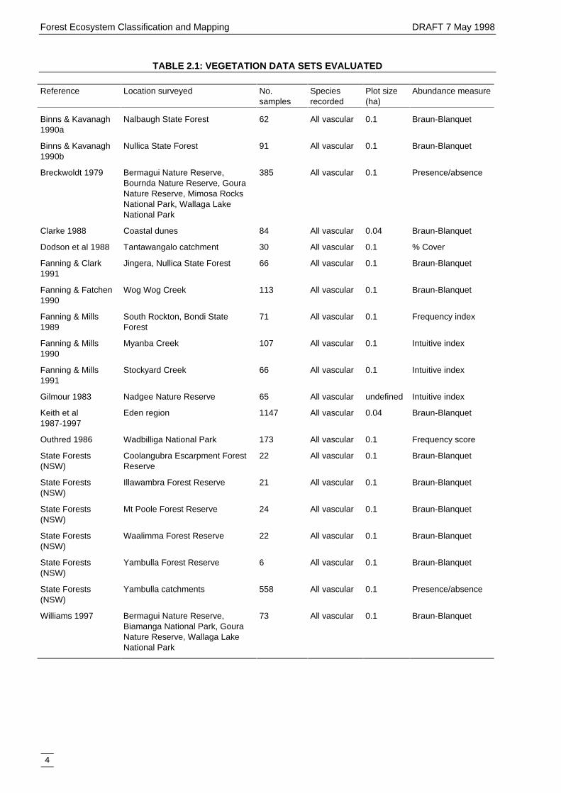
All available vegetation data were reviewed andevaluated for use in the Eden ComprehensiveRegional Assessment (Table 2.1). These dataoriginated from numerous surveys of localmanagement areas (for example, Gilmour 1983,Binns and Kavanagh 1990a) and from a regionalsurvey carried out in several phases between 1987and 1997 (Keith and Sanders 1990, Keith et al.1995).

A total of 3168 samples were evaluated, fromwhich 1590 were selected for analysis and eithermodelling or validation. All 3168 samples werelocated on the Australian Map Grid with aprecision of at least 100 m. The following criteriawere used to select samples of suitable quality foranalysis:

(I) Area of plot within the range 0.04 - 0.1hectares;

(II) Complete list of vascular plant specieswithin the plot;

(III) Species cover-abundance preferablyestimated on six-point Braun-Blanquetscale;

(IV) Assignable to a forest ecosystem with a highlevel of certainty.

The limits suggested in Criterion I were supportedby trial data analyses in which the outcome ofcluster analysis was not sensitive to variation insample size between 0.04 and 0.1 hectares. Allsamples met Criterion I except those of Gilmour(1983) for which the dimensions of plots were notrecorded. However, it is likely that most of thesesamples fell within the 0.04 - 0.1 hectares range(Gilmour, pers. comm.). All samples met CriterionII, although it is likely that a few inconspicuousspecies may have been overlooked in some

samples, particularly geophytes which may beabsent above ground during certain seasons oryears. A large number of additional samples werenot considered for analysis because they includedtree species only. Tree species make upapproximately 5% of the known vascular flora ofthe Eden region.

Approximately half of the samples had speciescover-abundance data on the six-point Braun-Blanquet scale (Poore 1955) and a further 173samples had species frequency scores based onnested quadrats (Outhred 1985). Criterion IIIexcluded from analysis 943 samples that hadspecies presence/absence data only (Breckwoldt1979, SFNSW unpublished) and 309 samples thathad qualitative species abundance classes (forexample, Gilmour 1983). In some surveys (forexample, Fanning and Mills 1990a), species wereassigned multiple abundance estimates forrespective strata, but no overall estimate for theplot. Criterion IV excluded from analysis a further326 samples that could not be assigned withacceptable certainty to vegetation classes definedby floristic analyses carried out previously on1066 samples (Keith et al. 1995).

The certainty of sample assignments wasdetermined by consensus among four alternativemultivariate methods (see below). The regionalcoverage of vegetation data was largely unaffectedby the exclusion of samples that were unsuitablefor analysis. Their exclusion was thereforeunlikely to have a major impact on samplestratification.


4

TABLE 2.1: VEGETATION DATA SETS EVALUATED

Reference Location surveyed No.samples

Speciesrecorded

Plot size(ha)

Abundance measure

Binns & Kavanagh1990a

Nalbaugh State Forest 62 All vascular 0.1 Braun-Blanquet

Binns & Kavanagh1990b

Nullica State Forest 91 All vascular 0.1 Braun-Blanquet

Breckwoldt 1979 Bermagui Nature Reserve,Bournda Nature Reserve, GouraNature Reserve, Mimosa RocksNational Park, Wallaga LakeNational Park

385 All vascular 0.1 Presence/absence

Clarke 1988 Coastal dunes 84 All vascular 0.04 Braun-Blanquet

Dodson et al 1988 Tantawangalo catchment 30 All vascular 0.1 % Cover

Fanning & Clark1991

Jingera, Nullica State Forest 66 All vascular 0.1 Braun-Blanquet

Fanning & Fatchen1990

Wog Wog Creek 113 All vascular 0.1 Braun-Blanquet

Fanning & Mills1989

South Rockton, Bondi StateForest

71 All vascular 0.1 Frequency index

Fanning & Mills1990

Myanba Creek 107 All vascular 0.1 Intuitive index

Fanning & Mills1991

Stockyard Creek 66 All vascular 0.1 Intuitive index

Gilmour 1983 Nadgee Nature Reserve 65 All vascular undefined Intuitive index

Keith et al1987-1997

Eden region 1147 All vascular 0.04 Braun-Blanquet

Outhred 1986 Wadbilliga National Park 173 All vascular 0.1 Frequency score

State Forests(NSW)

Coolangubra Escarpment ForestReserve

22 All vascular 0.1 Braun-Blanquet

State Forests(NSW)

Illawambra Forest Reserve 21 All vascular 0.1 Braun-Blanquet

State Forests(NSW)

Mt Poole Forest Reserve 24 All vascular 0.1 Braun-Blanquet

State Forests(NSW)

Waalimma Forest Reserve 22 All vascular 0.1 Braun-Blanquet

State Forests(NSW)

Yambulla Forest Reserve 6 All vascular 0.1 Braun-Blanquet

State Forests(NSW)

Yambulla catchments 558 All vascular 0.1 Presence/absence

Williams 1997 Bermagui Nature Reserve,Biamanga National Park, GouraNature Reserve, Wallaga LakeNational Park

73 All vascular 0.1 Braun-Blanquet

DRAFT 7 May 1998 Forest Ecosystem Classification and Mapping

5

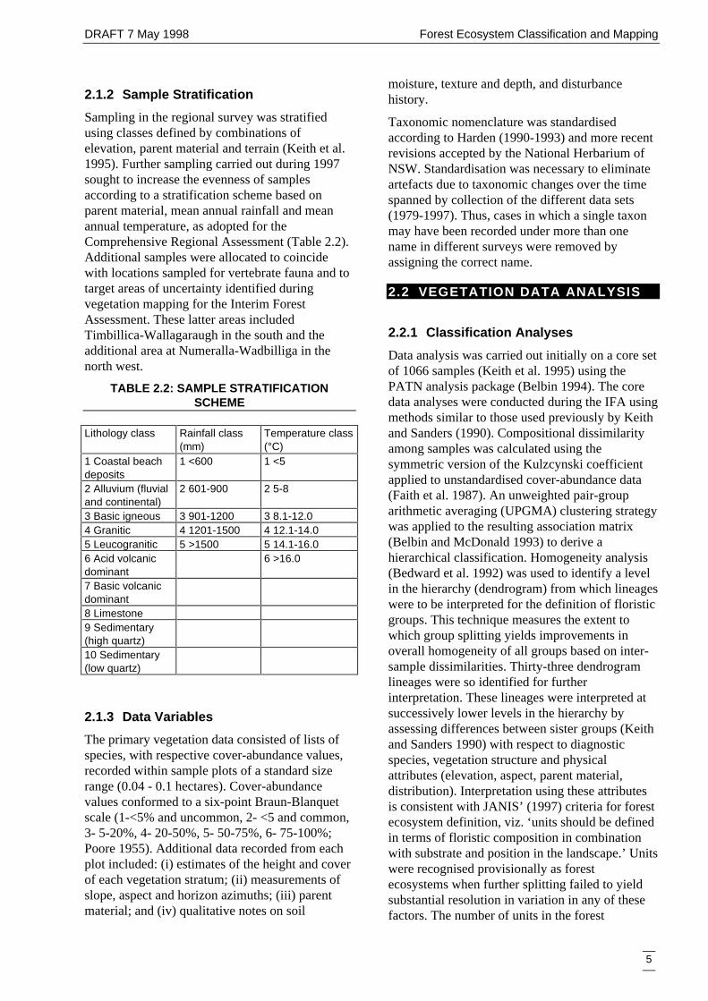
2.1.2 Sample Stratification

Sampling in the regional survey was stratifiedusing classes defined by combinations ofelevation, parent material and terrain (Keith et al.1995). Further sampling carried out during 1997sought to increase the evenness of samplesaccording to a stratification scheme based onparent material, mean annual rainfall and meanannual temperature, as adopted for theComprehensive Regional Assessment (Table 2.2).Additional samples were allocated to coincidewith locations sampled for vertebrate fauna and totarget areas of uncertainty identified duringvegetation mapping for the Interim ForestAssessment. These latter areas includedTimbillica-Wallagaraugh in the south and theadditional area at Numeralla-Wadbilliga in thenorth west.

TABLE 2.2: SAMPLE STRATIFICATIONSCHEME

Lithology class Rainfall class(mm)

Temperature class(°C)

1 Coastal beachdeposits

1 <600 1 <5

2 Alluvium (fluvialand continental)

2 601-900 2 5-8

3 Basic igneous 3 901-1200 3 8.1-12.04 Granitic 4 1201-1500 4 12.1-14.05 Leucogranitic 5 >1500 5 14.1-16.06 Acid volcanicdominant

6 >16.0

7 Basic volcanicdominant8 Limestone9 Sedimentary(high quartz)10 Sedimentary(low quartz)

2.1.3 Data Variables

The primary vegetation data consisted of lists ofspecies, with respective cover-abundance values,recorded within sample plots of a standard sizerange (0.04 - 0.1 hectares). Cover-abundancevalues conformed to a six-point Braun-Blanquetscale (1-<5% and uncommon, 2- <5 and common,3- 5-20%, 4- 20-50%, 5- 50-75%, 6- 75-100%;Poore 1955). Additional data recorded from eachplot included: (i) estimates of the height and coverof each vegetation stratum; (ii) measurements ofslope, aspect and horizon azimuths; (iii) parentmaterial; and (iv) qualitative notes on soil

moisture, texture and depth, and disturbancehistory.

Taxonomic nomenclature was standardisedaccording to Harden (1990-1993) and more recentrevisions accepted by the National Herbarium ofNSW. Standardisation was necessary to eliminateartefacts due to taxonomic changes over the timespanned by collection of the different data sets(1979-1997). Thus, cases in which a single taxonmay have been recorded under more than onename in different surveys were removed byassigning the correct name.

2.2 VEGETATION DATA ANALYSIS

2.2.1 Classification Analyses

Data analysis was carried out initially on a core setof 1066 samples (Keith et al. 1995) using thePATN analysis package (Belbin 1994). The coredata analyses were conducted during the IFA usingmethods similar to those used previously by Keithand Sanders (1990). Compositional dissimilarityamong samples was calculated using thesymmetric version of the Kulzcynski coefficientapplied to unstandardised cover-abundance data(Faith et al. 1987). An unweighted pair-grouparithmetic averaging (UPGMA) clustering strategywas applied to the resulting association matrix(Belbin and McDonald 1993) to derive ahierarchical classification. Homogeneity analysis(Bedward et al. 1992) was used to identify a levelin the hierarchy (dendrogram) from which lineageswere to be interpreted for the definition of floristicgroups. This technique measures the extent towhich group splitting yields improvements inoverall homogeneity of all groups based on inter-sample dissimilarities. Thirty-three dendrogramlineages were so identified for furtherinterpretation. These lineages were interpreted atsuccessively lower levels in the hierarchy byassessing differences between sister groups (Keithand Sanders 1990) with respect to diagnosticspecies, vegetation structure and physicalattributes (elevation, aspect, parent material,distribution). Interpretation using these attributesis consistent with JANIS’ (1997) criteria for forestecosystem definition, viz. ‘units should be definedin terms of floristic composition in combinationwith substrate and position in the landscape.’ Unitswere recognised provisionally as forestecosystems when further splitting failed to yieldsubstantial resolution in variation in any of thesefactors. The number of units in the forest


6

ecosystem classification was therefore limited bythe identification of prominent differences inspecies composition, vegetation structure andphysical habitat.

A nearest neighbour check was carried out toidentify samples that may have been misclassifiedduring the clustering procedure, an artefact thatmay sometimes occur in hierarchical clusteringstrategies (Belbin 1994). Samples with fewer thantwo of their five nearest neighbours within theprovisional unit to which they were allocated wereidentified for further evaluation. Alternativeallocations of these samples were considered byexamining the group affinities of nearestneighbours and respective values of structural andenvironmental variables.

To modify and refine the classification with newdata available since the IFA analysis, furtheranalyses were conducted during the CRA on anexpanded data set to assign new samples toexisting classification units and, where newvariation was apparent, define additional units.Four analyses were carried out to establishrelationships to the classification defined byanalysis of the core data. These included furthercluster and nearest neighbour analyses asdescribed previously, group centroid analyses andindicator species allocation analyses. Groupcentroid analyses were carried out using ALOC(Belbin 1992, 1994) to determine the five nearestgroup centroids to each new sample. Indicatorspecies allocation analyses allocated new samplesto classification units using the dendrogram as adecision rule structure for the presence or absenceof species (Bedward and Keith 1997). The methoddelivers an indeterminate result for samples withno informative species or where different speciessuggest conflicting information on groupmembership.

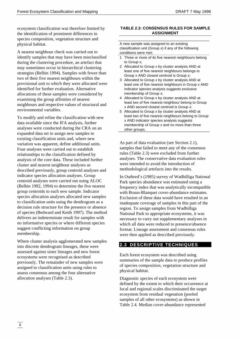
Where cluster analysis agglomerated new samplesinto discrete dendrogram lineages, these wereassessed against sister lineages and new forestecosystems were recognised as describedpreviously. The remainder of new samples wereassigned to classification units using rules toassess consensus among the four alternativeallocation analyses (Table 2.3).

TABLE 2.3: CONSENSUS RULES FOR SAMPLEASSIGNMENT

A new sample was assigned to an existingclassification unit (Group x) if any of the followingconditions were met:1 Three or more of its five nearest neighbours belong

to Group x;2 Allocated to Group x by cluster analysis AND at

least one of five nearest neighbours belongs toGroup x AND closest centroid is Group x;

3 Allocated to Group x by cluster analysis AND atleast one of five nearest neighbours in Group x ANDindicator species analysis suggests exclusivemembership of Group x;

4 Allocated to Group x by cluster analysis AND atleast two of five nearest neighbour belong to Groupx AND second closest centroid is Group x;

5 Allocated to Group x by cluster analysis AND atleast two of five nearest neighbours belong to Groupx AND indicator species analysis suggestsmembership of Group x and no more than threeother groups.

As part of data evaluation (see Section 2.1),samples that failed to meet any of the consensusrules (Table 2.3) were excluded from furtheranalyses. The conservative data evaluation ruleswere intended to avoid the introduction ofmethodological artefacts into the results.

In Outhred’s (1985) survey of Wadbilliga NationalPark species abundance was estimated using afrequency index that was analytically incompatiblewith Braun-Blanquet cover-abundance estimates.Exclusion of these data would have resulted in aninadequate coverage of samples in this part of theregion. To assign samples from WadbilligaNational Park to appropriate ecosystems, it wasnecessary to carry out supplementary analyses inwhich all data were reduced to presence/absenceformat. Lineage assessment and consensus ruleswere then applied as described previously.

2.3 DESCRIPTIVE TECHNIQUES

Each forest ecosystem was described usingsummaries of the sample data to produce profilesof species composition, vegetation structure andphysical habitat.

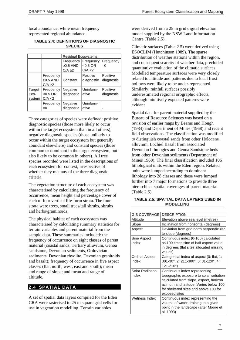
Diagnostic species of each ecosystem weredefined by the extent to which their occurrence atlocal and regional scales discriminated the targetecosystem from residual vegetation (pooledsamples of all other ecosystems) as shown inTable 2.4. Median cover-abundance represented


7

local abundance, while mean frequencyrepresented regional abundance.

TABLE 2.4: DEFINITIONS OF DIAGNOSTICSPECIES

Residual EcosystemsFrequency≥0.5 ANDC/A ≥2

Frequency<0.5 ORC/A <2

Frequency=0

Frequency≥0.5 ANDC/A ≥2

ConstantPositivediagnostic

Positivediagnostic

TargetEco-system

Frequency<0.5 ORC/A <2

Negativediagnostic

Uninform-ative

Positivediagnostic

Frequency=0

Negativediagnostic

Uninform-ative -

Three categories of species were defined: positivediagnostic species (those more likely to occurwithin the target ecosystem than in all others);negative diagnostic species (those unlikely tooccur within the target ecosystem but generallyabundant elsewhere) and constant species (thosecommon or dominant in the target ecosystem, butalso likely to be common in others). All treespecies recorded were listed in the descriptions ofeach ecosystem for context, irrespective ofwhether they met any of the three diagnosticcriteria.

The vegetation structure of each ecosystem wascharacterised by calculating the frequency ofoccurrence, mean height and percentage cover ofeach of four vertical life-form strata. The fourstrata were trees, small trees/tall shrubs, shrubsand herbs/graminoids.

The physical habitat of each ecosystem wascharacterised by calculating summary statistics forterrain variables and parent material from thesample data. These summaries included: thefrequency of occurrence on eight classes of parentmaterial (coastal sands, Tertiary alluvium, Genoasandstone, Devonian sediments, Ordoviciansediments, Devonian rhyolite, Devonian granitoidsand basalt); frequency of occurrence in five aspectclasses (flat, north, west, east and south); meanand range of slope; and mean and range ofaltitude.

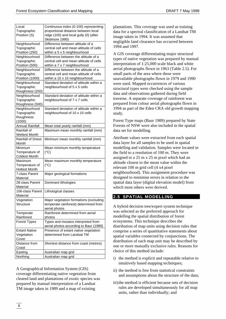
2.4 SPATIAL DATA

A set of spatial data layers compiled for the EdenCRA were rasterised to 25 m square grid cells foruse in vegetation modelling. Terrain variables

were derived from a 25 m grid digital elevationmodel supplied by the NSW Land InformationCentre (Table 2.5).

Climatic surfaces (Table 2.5) were derived usingESOCLIM (Hutchinson 1989). The sparsedistribution of weather stations within the region,and consequent scarcity of weather data, precludedquantitative evaluation of the climatic surfaces.Modelled temperature surfaces were very closelyrelated to altitude and patterns due to local frosthollows were likely to be under-represented.Similarly, rainfall surfaces possiblyunderestimated regional orographic effects,although intuitively expected patterns wereevident.

Spatial data for parent material supplied by theBureau of Resource Sciences was based on arevision of earlier maps by Beams and Hough(1984) and Department of Mines (1968) and recentfield observations. The classification was modifiedto distinguish coastal sands from other Holocenealluvium, Lochiel Basalt from associatedDevonian lithologies and Genoa Sandstone bedsfrom other Devonian sediments (Department ofMines 1968). The final classification included 106lithological units within the Eden region. Relatedunits were lumped according to dominantlithology into 28 classes and these were lumpedfurther into 7 major formations to provide threehierarchical spatial coverages of parent material(Table 2.5).

TABLE 2.5: SPATIAL DATA LAYERS USED INMODELLING

GIS COVERAGE DESCRIPTIONAltitude Elevation above sea level (metres)Slope Inclination from horizontal (degrees)Aspect Deviation from grid north perpendicular

to slope (degrees)Sine AspectIndex

Continuous index (0-100) calculatedas 100 times sine of half aspect valuein degrees (flat sites allocated missingvalues)

Ordinal AspectIndex

Categorical index of aspect (0: flat, 1:301-30°, 2: 211-300°, 3: 31-120°, 4:121-210°)

Solar RadiationIndex

Continuous index representingtopographic exposure to solar radiationcalculated from slope, aspect, horizonazimuth and latitude. Varies below 100for sheltered sites and above 100 forexposed sites

Wetness Index Continuous index representing thevolume of water draining to a givenpoint in the landscape (after Moore etal. 1993)


8

LocalTopographicPosition (S)

Continuous index (0-100) representingproportional distance between localridge (100) and local gully (0) (afterSkidmore 1990)

NeighbourhoodTopographicPosition (250)

Difference between altitude of acentral cell and mean altitude of cellswithin a 5 x 5 neighbourhood


Difference between the altitude of acentral cell and mean altitude of cellswithin a 7 x 7 neighbourhood


Difference between the altitude of acentral cell and mean altitude of cellswithin a 10 x 10 neighbourhood

NeighbourhoodTopographicRoughness (250)

Standard deviation of altitude within aneighbourhood of 5 x 5 cells

NeighbourhoodTopographicRoughness (500)


NeighbourhoodTopographicRoughness(1000)


Annual Rainfall Mean total yearly rainfall (mm)Rainfall ofWettest Month

Maximum mean monthly rainfall (mm)

Rainfall of DriestMonth

Minimum mean monthly rainfall (mm)

MinimumTemperature ofColdest Month

Mean minimum monthly temperature(°C)

MaximumTemperature ofHottest Month

Mean maximum monthly temperature(°C)

7-class ParentMaterial

Major geological formations


Dominant lithologies


Lithological classes

VegetationStructure

Major vegetation formations (excludingtemperate rainforest) determined fromaerial photos

TemperateRainforest

Rainforest determined from aerialphotos

Forest Types Types and mosaics interpreted fromaerial photos according to Baur (1989)

Extant NativeVegetationCover

Presence of extant native vegetationdetermined from Landsat TM

Distance fromCoast

Shortest distance from coast (metres)

Easting Australian map gridNorthing Australian map grid

A Geographical Information System (GIS)coverage differentiating native vegetation fromcleared land and plantations of exotic species wasprepared by manual interpretation of a LandsatTM image taken in 1989 and a map of existing

plantations. This coverage was used as trainingdata for a spectral classification of a Landsat TMimage taken in 1994. It was assumed thatnegligible land clearance has occurred between1994 and 1997.

A GIS coverage differentiating major structuraltypes of native vegetation was prepared by manualinterpretation of 1:25,000 scale black and whiteaerial photographs flown in 1963 (Table 2.5). Forsmall parts of the area where these wereunavailable photographs flown in 1979 and 1990were used. Mapped occurrences of variousstructural types were checked using the sampledata and observations gathered during fieldtraverse. A separate coverage of rainforest wasprepared from colour aerial photographs flown in1994 as part of the Eden CRA old growth mappingstudy.

Forest Type maps (Baur 1989) prepared by StateForests of NSW were also included in the spatialdata set for modelling.

Attribute values were extracted from each spatialdata layer for all samples to be used in spatialmodelling and validation. Samples were located inthe field to a resolution of 100 m. They wereassigned to a 25 m x 25 m pixel which had analtitude closest to the mean value within therelevant 100 m grid cell (4 x4 pixelneighbourhood). This assignment procedure wasdesigned to minimise errors in relation to thespatial data layer (digital elevation model) fromwhich most others were derived.

2.5 SPATIAL MODELLING

A hybrid decision tree/expert system techniquewas selected as the preferred approach formodelling the spatial distribution of forestecosystems. This technique describes thedistribution of map units using decision rules thatcomprise a series of quantitative statements aboutspatial variables connected by conjunctions. Thedistribution of each map unit may be described byone or more mutually exclusive rules. Reasons forchoice of this method include:

i) the method is explicit and repeatable relative tointuitively based mapping techniques;

ii) the method is free from statistical constraintsand assumptions about the structure of the data;

iii) the method is efficient because sets of decisionrules are developed simultaneously for all mapunits, rather than individually; and


9

iv) the method allows for intervention by expertsin an explicit manner through the choice anddesign of rules.

The main disadvantage of decision tree modelsrelative to parametric models (for example,generalised linear and additive models) is that theyutilise fewer and fewer samples as more variablesare fitted. Consequently, inadequate sampling ofenvironmental space may be more limiting, at leastsuperficially, for decision tree models.Comparative studies on the prediction ofdistributions of individual species suggest thatgeneralised linear models and generalised additivemodels return slightly more accurate predictionsthan decision tree models (Ferrier and Watson1997). However, these trials excluded expertintervention. No comparative studies have yetbeen carried out on the modelling of multi-speciesassemblages.

Interactive modelling software (ALBERO) wasdeveloped to explore and implement alternativesets of decision rules. The software generatesdecision rules by statistical induction andfacilitates expert intervention at various stages ofmodel development. At each node in the decisiontree, ALBERO displays all significant statementsdiscriminating different ecosystems by spatialvariables (within a user-specified critical value)and nominates appropriate thresholds fordiscrimination. Significance is calculated using theChi-squared statistic. For continuous and ordinalvariables, nodes are always split dichotomously atthe significant value closest to the midpoint ofvariation. Non-ordinal categorical variables willsplit nodes into as many branches as account forsignificant discrimination of ecosystems. Wheretwo or more spatial variables discriminateecosystems significantly, the user chooses aselection. Users may reduce the critical value tohelp make a choice. A decision rule (ie. branch ofthe decision tree) is complete when there are nofurther significant splits at the nominated criticalvalue.

ALBERO accommodates explicit expertintervention in the modelling process by offering achoice between multiple significant variables ateach node, facilitating exploration of alternativetree structures, allowing non-significant splits tobe forced, and allowing definition of data-freeterminal nodes. The latter facility accommodatesqualitative observations by experts where noquantitative data are available.

A decision-tree model of forest ecosystems in theEden region was developed by selectingsignificant regional-scale spatial variables (parentmaterial, rainfall and temperature) at early stagesof tree construction, then turning to local-scalevariables (for example, terrain) to discriminatesmaller groups of samples representing differentecosystems. The model was developed iterativelyby checking ecosystem distributions predicted byparticular sets of rules and adjusting tree structureas necessary (see Section 2.7). Terminal nodeswere allocated to the ecosystem represented by thegreatest number of samples. Where there was a tie,expert knowledge was applied to choose the mostlikely option.

2.6 MAP COMPILATION

The final set of decision rules was applied to thefull set of spatial data layers to allocate all 25 mgrid cells in the study area to a forest ecosystemclass. The resulting map represented the pre-1750distribution of ecosystems. This was cut using theLandsat coverage of extant native vegetation cover(Table 2.5) to derive extant distributions of forestecosystems.

2.7 MAP VALIDATION

2.7.1 Qualitative Checking

Checking procedures were incorporated into thedevelopment of the map. The decision-tree modelwas broken down into manageable components forproofing. The checking process was carried out byan experienced field botanist (David Keith) andconsisted of the following steps.

1. A small number of rules were extracted fromthe model and implemented on the spatial datato display the distribution of respective forestecosystems.

2. The mapped distributions of ecosystems wereexamined in relation to the regional distributionof their samples.

3. The fine scale distributions of ecosystems wereexamined with reference to topographic mapsto determine whether appropriate landscaperelationships were reflected (for example, thatsheltered gullies generally support eithersimilar or more mesic vegetation than adjacentridges, but not less mesic vegetation).


10

4. The sources of all identified anomalies weretraced to particular nodes in the decision treeand the sample data were examined to explorealternative rule pathways below the nodeidentified.

5. The model and map were revised and proofingsteps 1-5 were repeated until all identifiedanomalies were resolved.

When model development was well advanced,further refinements were sought from a secondexperienced field botanist (Doug Binns, StateForests of NSW).

2.7.2 Accuracy Quantification

Approximately 10% of the 1590 samples selectedfor data analysis were withheld from modelling foraccuracy quantification. These validation sampleswere used to test model predictions againstindependent observations at a spatial scale relevantto map usage in the CRA. Validation samples wereselected at random from all forest ecosystemsexcluding those with less than 20 samples so asnot to unduly constrain modelling options forthese less common units. Many of the lesswidespread ecosystems excluded from validationwere modelled principally using aerial photographinterpreted spatial layers (for example, rainforests,heaths, swamps). It was thus assumed that theywere mapped with reasonable confidence.

The aim of accuracy quantification was todetermine the likelihood that selection of an areato represent a given ecosystem in a reserveactually contained the ecosystem predicted on themap. Planning units used for reserve selection inthe Eden CRA varied in size from approximately20 hectares to 240 hectares. Validation sampleswere thus compared to mapped ecosystems withinneighbourhoods of 95 hectares to determine errorrates at a spatial scale relevant to the planningexercise. The percentage of correct matches wasrecorded as an estimate of map accuracy.

11

3. RESULTS ANDDISCUSSION

3.1 FOREST ECOSYSTEMCLASSIFICATION

Homogeneity analysis suggested that at least 33groups were required to summarise majorvariation in the floristic data. Further interpretationof these 33 lineages resulted in recognition of 61forest ecosystems. A further six ecosystems wererecognised in the analysis of presence/absencedata including samples from Wadbilliga NationalPark. Nine additional unsampled units includingeight estuarine wetlands and one grassland werealso recognised as forest ecosystems and describedqualitatively. Appendix 1 describes the floristiccomposition, vegetation structure, physical habitatand distribution of samples for each forestecosystem. Approximate floristic relationshipsbetween forest ecosystems are shown in thesimplified dendrogram in Figure 3.1.

A number of dendrogram lineages identified fromHomogeneity analysis were not split further. Anexample of one lineage in which splitting resolvedcomplex variation into six forest ecosystems isdescribed in the following steps (refer to first sixecosystems in Figure 3.1).

1. The parent lineage contains 90 samples with adiverse range of dry forest species. Samplesencompass altitudinal range of 15 -915m on arange of granitoid, sandstone, mudstone andalluvial parent materials, across all aspects onflat and dissected terrain. Samples aredistributed throughout the coast and southernparts of hinterland and tableland range.

2. The first split segregated a group of samplesrestricted to sandstone on steep northern andwestern aspects of Mt Imlay, NungattaMountain and Bondi Gulf at 330-750melevation. Samples indicate a forest less than 20m tall dominated by Eucalyptus agglomerata

and prominent ground stratum. Further splittingfailed to resolve substantial variation withinthis group. It was therefore recognised andmapped as Ecosystem 50.

3. The second split resulted in two further groups.The first of these included samples distributedwidely on coastal ranges and inland mountainswhich, when split again, yielded one subgroupdominated by E. sieberi and largely confined totonalite lithology in the Mumbulla Mountainarea, and another subgroup dominated by E.agglomerata, E. sieberi and Allocasuarinalittoralis restricted to sedimentary lithologieson coastal and hinterland ranges. Furthersplitting failed to resolve substantial variationwithin these subgroups which were recognisedand mapped as Ecosystems 48 and 49,respectively.

4. The remaining sample groups in the lineagewere resolved into three Ecosystems in asimilar manner. They were: 46A (low forestdominated by E. consideniana restricted togranitoids and Tertiary alluvium in theTimbillica area); 46B (taller forest dominatedby E. gummifera and E. sieberi confined tosediments and Tertiary alluvium on the coastalstrip); and 47 (taller forest dominated byAngophora floribunda and E. sieberi confinedto sediments south of Pambula).

Alternative interpretations of the hierarchyyielding greater and fewer ecosystem units wereconsidered in the manner described above. It wasdecided and ultimately agreed by SteeringCommittee that the final classification of 76ecosystems (47 eucalypt-dominated) provided aconservative summary of vegetation and habitatvariation in the region and a reasonableinterpretation of the JANIS (1996) definition offorest ecosystems. The conservative nature of the


12

classification is demonstrated by a comparisonwith existing forest type mapping that coveredapproximately one-quarter (200 000 hectares) ofthe Eden CRA region. This classificationaddresses only variation in composition of thedominant tree stratum and, compared to the forestecosystem classification, comprises approximatelytwice as many units (c. 150) in a smaller area.

Four of the 76 ecosystems were restricted toestuaries below low tide mark (sea grassmeadows) and consequently were not mapped. Afurther four ecosystems were estuarine wetlandsassociated with the high tide mark. Of theremainder, 47 ecosystems were forests dominatedby eucalypts, six were rainforests or scrubs withrainforest affinities, 12 were shrublands orheathlands and three were swamps.

Major groups of ecosystems include dry eucalyptforests with shrub-dominated understoreys,intermediate forests and riparian vegetation, dryeucalypt forests with grass-dominatedunderstoreys, shrub-dominated heathlands, rockscrubs and swamps, rainforests, dry eucalyptforests with understoreys dominated by grasses inthe Bega and Towamba Valleys, and vegetation ofheadlands and beaches.

The main changes to the classification relative tothat described by Keith et al. (1995) are related tothe addition of 140 000 hectares to the north-westthe study area (Numeralla-Wadbilliga). Sixadditional forest ecosystems (W1-W6) arerestricted to dissected sedimentary terrain inWadbilliga National Park. One additionalecosystem (22B) is restricted to the Numerallaarea. One additional ecosystem (46A) occurs inthe Timbillica area. Previously, there had beeninsufficient data to distinguish this unit from otherdry lowland eucalypt forest (46B). The other 68ecosystems remain unaltered from the IFAanalysis (Keith et al. 1996) and retain the samenumbering system.

Ecological gradients and biogeographicalrelationships of vegetation in the Eden region arereviewed by Keith and Sanders (1990).

3.2 FOREST ECOSYSTEM MAP

A hybrid decision tree model/expert systemcomprising 400 rules was developed iteratively asdescribed previously. The highest order statementin each rule referred to major structural formations(rainforest, eucalypt forest, tall scrub, riparian

vegetation, heath, grassland, treeless swamp andestuarine vegetation). Eucalypt forests weresubsequently distinguished by parent material andthen climatic variables. Lower order statements inrules describing the distribution of eucalypt-dominated ecosystems were, in most cases, basedon local terrain, geology and aerial photo-interpreted variables. The decision rules wereimplemented on the spatial data layers to producethe forest ecosystem map.

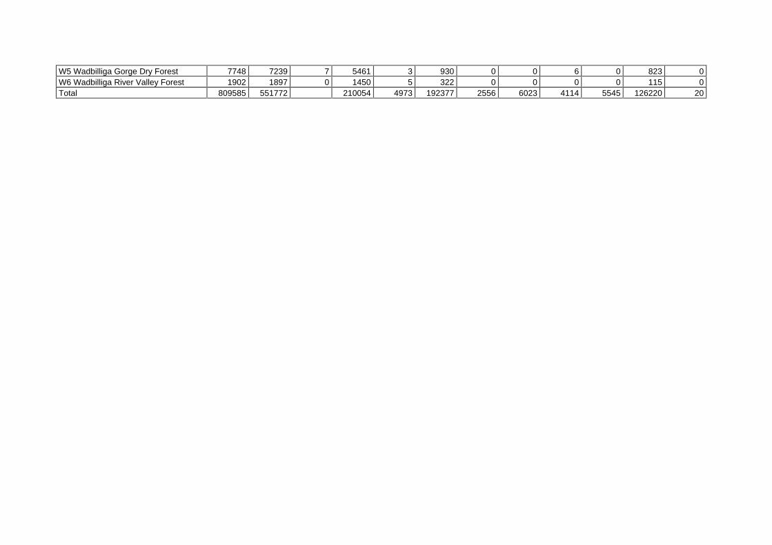
Forest Ecosystems 61 and 62 were mapped as amosaic because stands of Ecosystem 62 wererestricted to narrow beach strands and too small tomap separately from adjoining stands ofEcosystem 61 at 25 m pixel scale. Appendix 1shows the location of samples assigned to eachecosystem. The mapped extent of pre-1750 and1997 area of each ecosystem is given in Table 3.1.The extant area of each ecosystem on differentland tenures is also given in Table 3.1. Theecosystems most depleted by clearing are in theBega and Towamba valleys (18, 19, 20 , 21, 39and 40), on the Monaro Tableland (22A, 22B,23A, 23B, 24 and 59) and along the coastal strip(36 and 60). The Eden Forest Ecosystem Map isavailable under licence from the NSW NationalParks and Wildlife Service. The metadatastatement is reproduced in Appendix 2.

3.3 MAP VALIDATION

3.3.1 Qualitative Checking

Qualitative checking revealed a number ofmapping anomalies generated by the first iterationof decision rules. For example, some stands ofForest Ecosystem 58 (Swamp Forest) had initiallybeen mapped along contours in the south-westernpart of the region. Comments on the field datasheets and our recollections from the fieldindicated that this type of vegetation occurs onflats along drainage lines. The anomaly wasrectified by replacing maximum temperature andelevation with topographic roughness and wetnessindex in the appropriate decision rule. Otheridentified anomalies were similarly rectified.

3.3.2 Accuracy Quantification

One hundred and forty randomly selected sampleswere withheld from modelling for accuracyquantification. These samples representedEcosystems 13, 14, 15, 31, 32, 33, 34, 37, 42, 46A,46B, 47, 49, 61, 62, W1 and W6. Ecosystems


13

assigned by floristic analysis to samples matchedecosystems mapped within 95 hectares circularneighbourhoods of the sample location in 92% ofcases. This suggests that 92% of planning unitswill actually contain a forest ecosystem that ismapped within their boundary for which they maybe selected to represent in reserves.


14

FIGURE 3.1: DENDROGRAM SHOWING FLORISTIC RELATIONSHIPS BETWEEN FORESTECOSYSTEMS.

48________________________ 49_______________________|__46A__________________ |46B_________________|_____ | 47______________________|__|_ 50__________________________|__________ 44__________________ | 43_________________|___ | 45____________________|______ | 42__________________________|__ | 41____________________________|_______|____________ 32________________________________ | 33_______________________________|______ | 34_________________________ | | 2________________________|__ | | 35__________________________|______ | | 36_____________________________ | | | 37____________________________|___|__ | | 63_______________________________ | | | 38____________________________ | | | | 39_______________________ | | | | | 40______________________|____|__|___|__|____ | 31______________________ | | 30_____________________|_ | | 29______________________|__ | | 28________________________|________ | | 26______________________ | | | 25_____________________|____ | | |23B______________ | | | |22A_________ | | | | |22B________|____|___ | | | | 24________________|________|__ | | | 27___________________________|____|________|______|_______ 52________________________ | 51_______________________|_____________________ | 59_______________________________ | | 58______________________________|___________ | | 56_________________________ | | | 55___________________ | | | | 54__________________|_____|________ | | | 57________________________________|_____ | | | 53_____________________________________|___|__|______ | 3____________________________ | | 1___________________________|___ | | 4______________________________|______ | | 6_____________ | | | 7____________|_______________________|_____________|____|____ 10_____________________________ | 9________________________ | | 8_______________________|____|____ | 11________________________________|______________ | 12______________________ | | 13_____________________|____ | | 14_________________________|_______ | | 15______________________________ | | | 16_________________________ | | | | 17________________________|____|__|_____________|____________|_____________ 18___________________ | 19__________________|__________ | 20___________________________ | | 21__________________________|_|___________________________________________|__________________ 61__________________________________________________ | 62_________________________________________________|________________________________________|

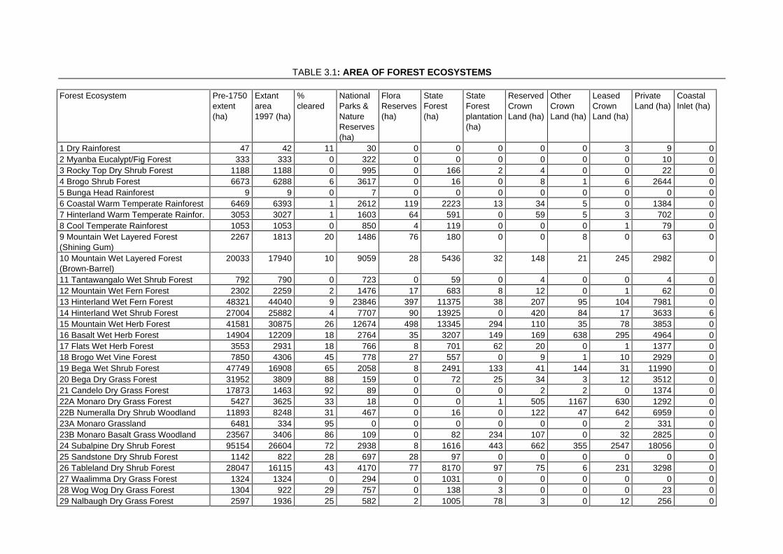
TABLE 3.1: AREA OF FOREST ECOSYSTEMS

Forest Ecosystem Pre-1750extent(ha)

Extantarea1997 (ha)

%cleared

NationalParks &NatureReserves(ha)

FloraReserves(ha)

StateForest(ha)

StateForestplantation(ha)

ReservedCrownLand (ha)

OtherCrownLand (ha)

LeasedCrownLand (ha)

PrivateLand (ha)

CoastalInlet (ha)

1 Dry Rainforest 47 42 11 30 0 0 0 0 0 3 9 02 Myanba Eucalypt/Fig Forest 333 333 0 322 0 0 0 0 0 0 10 03 Rocky Top Dry Shrub Forest 1188 1188 0 995 0 166 2 4 0 0 22 04 Brogo Shrub Forest 6673 6288 6 3617 0 16 0 8 1 6 2644 05 Bunga Head Rainforest 9 9 0 7 0 0 0 0 0 0 0 06 Coastal Warm Temperate Rainforest 6469 6393 1 2612 119 2223 13 34 5 0 1384 07 Hinterland Warm Temperate Rainfor. 3053 3027 1 1603 64 591 0 59 5 3 702 08 Cool Temperate Rainforest 1053 1053 0 850 4 119 0 0 0 1 79 09 Mountain Wet Layered Forest(Shining Gum)

2267 1813 20 1486 76 180 0 0 8 0 63 0

10 Mountain Wet Layered Forest(Brown-Barrel)

20033 17940 10 9059 28 5436 32 148 21 245 2982 0

11 Tantawangalo Wet Shrub Forest 792 790 0 723 0 59 0 4 0 0 4 012 Mountain Wet Fern Forest 2302 2259 2 1476 17 683 8 12 0 1 62 013 Hinterland Wet Fern Forest 48321 44040 9 23846 397 11375 38 207 95 104 7981 014 Hinterland Wet Shrub Forest 27004 25882 4 7707 90 13925 0 420 84 17 3633 615 Mountain Wet Herb Forest 41581 30875 26 12674 498 13345 294 110 35 78 3853 016 Basalt Wet Herb Forest 14904 12209 18 2764 35 3207 149 169 638 295 4964 017 Flats Wet Herb Forest 3553 2931 18 766 8 701 62 20 0 1 1377 018 Brogo Wet Vine Forest 7850 4306 45 778 27 557 0 9 1 10 2929 019 Bega Wet Shrub Forest 47749 16908 65 2058 8 2491 133 41 144 31 11990 020 Bega Dry Grass Forest 31952 3809 88 159 0 72 25 34 3 12 3512 021 Candelo Dry Grass Forest 17873 1463 92 89 0 0 0 2 2 0 1374 022A Monaro Dry Grass Forest 5427 3625 33 18 0 0 1 505 1167 630 1292 022B Numeralla Dry Shrub Woodland 11893 8248 31 467 0 16 0 122 47 642 6959 023A Monaro Grassland 6481 334 95 0 0 0 0 0 0 2 331 023B Monaro Basalt Grass Woodland 23567 3406 86 109 0 82 234 107 0 32 2825 024 Subalpine Dry Shrub Forest 95154 26604 72 2938 8 1616 443 662 355 2547 18056 025 Sandstone Dry Shrub Forest 1142 822 28 697 28 97 0 0 0 0 0 026 Tableland Dry Shrub Forest 28047 16115 43 4170 77 8170 97 75 6 231 3298 027 Waalimma Dry Grass Forest 1324 1324 0 294 0 1031 0 0 0 0 0 028 Wog Wog Dry Grass Forest 1304 922 29 757 0 138 3 0 0 0 23 029 Nalbaugh Dry Grass Forest 2597 1936 25 582 2 1005 78 3 0 12 256 0

30 Wallagaraugh Dry Grass Forest 1663 914 45 273 0 400 13 1 0 0 228 031 Hinterland Dry Grass Forest 32925 27586 16 9319 60 13104 282 107 2 49 4676 032 Coastal Dry Shrub Forest 24521 23401 5 5919 41 11956 0 861 173 25 4441 033 Coastal Dry Shrub Forest 16298 16136 1 7072 6 7930 19 15 33 5 1061 034 Brogo Dry Shrub Forest 16155 14155 12 4111 0 5137 0 219 113 46 4528 335 Escarpment Dry Grass Forest 34577 22007 36 6231 251 3731 411 390 70 103 10840 036 Dune Dry Shrub Forest 1023 604 41 240 0 5 0 91 24 0 245 237 Coastal Dry Shrub Forest 16153 15147 6 4770 285 8173 0 132 39 26 1722 138 Southern Riparian Scrub 611 516 16 128 5 197 9 0 0 0 178 039 Northern Riparian Scrub 761 485 36 39 0 13 6 0 2 2 426 040 Riverine Forest 81 65 19 0 0 0 0 0 0 0 65 041 Mountain Dry Shrub Forest 1865 1864 0 1361 22 418 0 3 0 6 54 042 Coastal Dry Shrub Forest 22044 21556 2 4596 1010 15215 2 20 22 2 687 043 Mountain Dry Shrub Forest 2492 2479 1 2229 0 96 0 0 0 0 154 044 Foothills Dry Shrub Forest 3326 3142 6 2037 22 970 67 0 0 0 46 045 Mountain Dry Shrub Forest 2024 1915 5 858 33 648 17 0 0 1 359 046A Timbillica Dry Shrub Forest 22917 22792 1 1164 610 20497 13 11 0 0 497 046B Lowland Dry Shrub Forest 15978 15121 5 6384 0 5941 8 521 145 0 2127 247 Eden Dry Shrub Forest 17797 17141 4 11727 108 4098 16 134 83 13 965 048 Bega Dry Shrub Forest 4497 4455 1 3167 0 971 0 69 17 0 231 049 Coastal Dry Shrub Forest 32334 31837 2 6739 794 21042 1 54 61 1 3150 050 Genoa Dry Shrub Forest 3702 3026 18 1996 42 776 11 0 0 1 200 051 Rock Shrub 51 51 0 22 19 10 0 0 0 0 0 052 Mountain Rock Scrub 202 202 0 168 18 10 1 0 0 0 6 053 Montane Heath 1751 1350 23 388 0 5 19 197 215 121 407 054 Mountain Nadgee Heath 371 371 0 365 0 6 0 0 0 0 0 055 Coastal Lowland Heath 1676 1630 3 1490 0 37 0 1 9 0 93 056 Swamp Heath 385 385 0 12 1 362 0 0 0 0 10 057 Lowland Swamp 2010 1892 6 908 145 676 0 12 5 3 141 058 Swamp Forest 1080 953 12 373 6 529 9 1 0 0 36 059 Sub-Alpine Bog 6636 1869 72 492 1 259 40 14 17 60 989 060 Floodplain Wetlands 9421 3281 65 296 0 240 0 187 137 10 2417 061 Coastal Scrub 2273 1505 34 1128 0 4 0 78 72 0 222 163 Estuarine Wetland (scrub) 3028 932 69 91 0 17 0 49 33 3 741 264 Saltmarsh 370 296 20 47 0 3 0 45 54 15 129 366 Estuarine Wetland (mangrove) 56 38 31 0 0 0 0 8 5 0 25 0W1 Wadbilliga Dry Shrub Forest 27352 27341 0 26747 0 237 0 0 109 39 205 0W2 Wadbilliga Range Ash Forest 1007 1007 0 1007 0 0 0 0 0 0 0 0W3 Wadbilliga Mallee Heath 3085 3085 0 3060 0 0 0 0 0 2 24 0W4 Wadbilliga Range Wet Forest 3501 3214 8 2536 0 111 0 48 51 109 343 0

W5 Wadbilliga Gorge Dry Forest 7748 7239 7 5461 3 930 0 0 6 0 823 0W6 Wadbilliga River Valley Forest 1902 1897 0 1450 5 322 0 0 0 0 115 0Total 809585 551772 210054 4973 192377 2556 6023 4114 5545 126220 20


18

4. REFERENCES

Austin, M. P. and Margules, C. R. (1986).Assessing representativeness. In: Usher, M. B.(ed.), Wildlife Conservation evaluation, pp. 45-67. Chapman and Hall, London.

Baur, G. N. (1989). Forest types of New SouthWales. Research Note 17. Forestry Commissionof NSW

Beams, S. D. and Hough, D. J. (1984).Explanatory notes to accompany geological mapof the Eden forestry region, NSW Miscellaneouspaper, Forestry Commission of NSW.

Bedward, M. and Keith, D. A. (1997). ISALOC:Indicator species allocation analysis. NSWNational Parks and Wildlife Service, unpublishedreport.

Bedward, M., Keith, D. A. and Pressey, R. L.(1992). Homogeneity analysis: assessing theutility of classifications and maps of naturalresources. Australian Journal of Ecology 17: 133-139.

Belbin, L. (1992). Comparing two sets ofcommunity data: A method for testing reserveadequacy. Australian Journal of Ecology 17, 255-262.

Belbin, L. (1994). PATN. Pattern analysispackage. CSIRO, Canberra.

Belbin, L. and McDonald, C. (1993). Comparingthree classification strategies for use in ecology.Journal of Vegetation Science 4, 341-348.

Binns, D. and Kavanagh, R. P. (1990a). Flora andfauna survey of Nalbaugh State Forest (Part)Bombala District, Eden region, south-easternNSW. NSW Forestry Commission ForestResources Series No. 9.

Binns, D. and Kavanagh, R. P. (1990b). Flora andfauna survey, Nullica State Forest, Eden district,Eden region. NSW Forestry Commission ForestResources Series No. 10.

Breckwoldt, R. (1979). A preliminary vegetationsurvey of Goura, Bermagui and Bournda NatureReserves, and Mimosa Rocks and Wallaga LakeNational Parks. Report to NSW NPWS.

Clarke, P. J. (1988). Coastal dune vegetation ofNSW. Report of the University of Sydney andSoil Conservation of NSW joint research project.

Commonwealth of Australia (1991). NationalForest Policy Statement: a new focus forAustralia’s forests. Advance Press, Perth.

Commonwealth of Australia (1995). Australia’sNational Biodiversity Strategy. AustralianGovernment Publishing Service, Canberra.

Department of Mines (1968). Bega 1:250,000geological map sheet.

Dodson, J. R., Kodela, P. G. and Myers, C. A.(1988). Vegetation survey of the Tantawangaloresearch catchments in the Eden Forestry region,NSW. NSW Forestry Commission ForestResources Series No. 4.

Faith, D. P., Minchin, P. R. and Belbin, L. (1987).Compositional dissimilarity as a robust measureof ecological distance. Vegetatio 69, 57-66.

Fanning, F. D. and Clark, S. S. (1991). Flora andfauna survey of Jingo Creek Catchment, NullicaState Forest, Eden Region. NSW ForestryCommission Forest Resources Series No. 14.

Fanning, F. D. and Fatchen, T. J. (1990). Theupper Wog Wog river catchment of Coolangubraand Nalbaugh State Forest, (Mines road area)NSW. NSW Forestry Commission ForestResources Series No. 12.

Fanning, F. D. and Mills, K. (1989). Naturalresource survey of the southern portion ofRockton section, Bondi State Forest. NSWForestry Commission Forest Resources SeriesNo. 6.

Fanning, F. D. and Mills, K. (1990). The MyanbaCreek catchment, Coolangubra State Forest. NSW


19

Forestry Commission Forest Resources SeriesNo. 11.

Fanning, F. D. and Mills, K. (1991). TheStockyard Creek catchment of Coolangubra StateForest. NSW Forestry Commission ForestResources Series No. 13.

Ferrier, S. and Watson, G. (1997). An evaluationof the effectiveness of environmental surrogatesand modelling techniques in predicting thedistribution of biological diversity. Report to theBiodiversity Convention and Strategy Section ofthe Biodiversity Group, Environment Australia

Gilmour, P. (1983). Vegetation survey of NadgeeNature Reserve. NSW NPWS unpublished report.

Harden, G. (1990-93). Flora of New South Wales.Volumes 1-4. University of New South WalesPress, Kensington.

Hutchinson, M. F. (1989). A new objectivemethod for spatial interpolation of meteorologicalvariables from irregular networks applied to theestimation of monthly mean solar radiation,temperature, precipitation and windrun. CSIRODivision of Water Resources TechnicalMemorandum 89/5, pp 104.

JANIS (1997). Proposed Nationally AgreedCriteria for the Establishment of aComprehensive, Adequate and RepresentativeReserve System for Forests in Australia. A reportby the Joint ANZECC/MCFFA National ForestPolicy Statement Implementation Sub-committee(JANIS).

Keith, D. A., Bedward, M. and Smith, J. (1995).Vegetation of the South East Forests of NewSouth Wales. NSW National Parks and WildlifeService, unpublished report.

Keith, D. A. and Sanders, J . M.(1990).Vegetation of the Eden region, South-eastern Australia: species composition, diversityand structure. Journal of Vegetation Science 1,203-232.

Moore, I. P. D., Gessler, P. E., Nielsen, G. A. andPeterson, G. A. (1993). Soil attribute predictionusing terrain analysis. Soil Science Society ofAmerica Journal 57, 443-452.

Noss, R. F. (1987). From plant communities tolandscapes in conservation inventories: a look atthe Nature Conservancy (USA). BiologicalConservation. 41, 11-37.

Outhred, R. (1986). Vegetation survey ofWadbilliga National Park. Data supplied toNPWS by surveyor.

Poore, M. E. D. (1955). The use ofphytosociological methods in ecologicalinvestigations. I. The Braun-blanquet system.Journal of Ecology 43, 226-244.

RACAC (1996). Interim forest assessment for theEden region, New South Wales. Resource andConservation Assessment Council.

Skidmore, A. K. (1990). Terrain position asmapped from a gridded digital elevation model.International Journal of Geographic InformationSystems 4, 33-49.

Williams, J. (1997). Vegetation survey ofBermagui Nature Reserve, Biamanga NationalPark, Goura Nature Reserve and WallagaNational Park. Report to NSW NPWS.

20

5. APPENDIX

5.1 DESCRIPTION OF FORESTECOSYSTEMS

The following tables contain tables summarisingdata, where available, on species composition,vegetation structure and physical habitat. Mapsshow distribution of samples and photographsindicate typical visual appearance.

Nomenclature follows Harden (Flora of NewSouth Wales, University of New South WalesPress , Kensington, 1990-1993).

Diagnostic species: Positive diagnostic speciesare those with a higher frequency (proportion ofsamples in which they are present) and highermedian cover abundance among the samples of aparticular forest ecosystem than in all othersamples combined. Negative diagnostic speciesare those with the reverse pattern of occurrence(that is, widespread species that are absent fromthe target ecosystem). Frequent species areneither positive or negative diagnostic, but have ahigh frequency among the samples of a particularforest ecosystem, irrespective of their frequencyamong all other samples combined. Coverabundance estimates are medians with inter-quartile ranges in parentheses.

Forest Ecosystem Classification and Mapping for the … · forest ecosystem classification and...

Documents

Transcript of Forest Ecosystem Classification and Mapping for the … · forest ecosystem classification and...