Forecasting the Volatility of the Dow Jones Islamic Stock ... · forecasting of the process of...
28
University of Pretoria Department of Economics Working Paper Series Forecasting the Volatility of the Dow Jones Islamic Stock Market Index: Long Memory vs. Regime Switching Adnen Ben Nasr Universite de Tunis Thomas Lux University of Kiel and University Jaume I Ahdi N. Ajmi Salman bin Abdulaziz University Rangan Gupta University of Pretoria Working Paper: 2014-12 March 2014 __________________________________________________________ Department of Economics University of Pretoria 0002, Pretoria South Africa Tel: +27 12 420 2413
Transcript of Forecasting the Volatility of the Dow Jones Islamic Stock ... · forecasting of the process of...

University of Pretoria
Department of Economics Working Paper Series
Forecasting the Volatility of the Dow Jones Islamic Stock Market Index: Long
Memory vs. Regime Switching Adnen Ben Nasr Universite de Tunis Thomas Lux University of Kiel and University Jaume I
Ahdi N. Ajmi Salman bin Abdulaziz University
Rangan Gupta University of Pretoria
Working Paper: 2014-12
March 2014
__________________________________________________________
Department of Economics
University of Pretoria
0002, Pretoria
South Africa
Tel: +27 12 420 2413

Forecasting the Volatility of the Dow Jones Islamic
Stock Market Index: Long Memory vs. Regime
Switching∗
Adnen Ben Nasr,† Thomas Lux,‡ Ahdi Noomen Ajmi § Rangan Gupta ¶
Abstract
The financial crisis has fueled interest in alternatives to traditionalasset classes that might be less affected by large market gyrations and,thus, provide for a less volatile development of a portfolio. One attemptat selecting stocks that are less prone to extreme risks, is obeyance ofIslamic Sharia rules. In this light, we investigate the statistical prop-erties of the DJIM index and explore its volatility dynamics using anumber of up-to-date statistical models allowing for long memory andregime-switching dynamics. We find that the DJIM shares all stylizedfacts of traditional asset classes, and estimation results and forecastingperformance for various volatility models are also in line with prevalentfindings in the literature. Overall, the relatively new Markov-switchingmultifractal model performs best under the majority of time horizonsand loss criteria. Long memory GARCH-type models always improveupon the short-memory GARCH specification and additionally allow-ing for regime changes can further improve their performance.
JEL Classification: G15, G17, G23Keywords: islamic finance, volatility dynamics, long memory, multifrac-tals.
∗Thomas Lux gratefully aknowledges financial support from the Spanish Ministry ofScience and Innovation (ECO2011-23634), from Universitat Jaume I (P1.1B2012-27), andfrom the European Union 7th Framework Programme, under grant agreement no. 612955†BESTMOD, Institut Superieur de Gestion de Tunis, Universite de Tunis, Tunisia.
Email: [email protected]‡Department of Economics, University of Kiel, Germany & Banco de Espana Chair in
Computational Economics, University Jaume I, Castellon, Spain.§College of Sciences and Humanities in Slayel, Salman bin Abdulaziz University, King-
dom of Saudi Arabia. Email: [email protected]¶Department of Economics, University of Pretoria, South Africa. Email: ran-
1

1 Introduction
The recent global financial crisis has exerted enormous negative impacts
on conventional institutions and markets. Hence, a need has been felt for
exploring alternatives to conventional financial practices that allow to reduce
investment risks, increase returns, enhance financial stability, and reassure
investors and financial markets. Given this, following the crisis, one has
observed a renewed interest in Islamic finance,1 based on Sharia rules, as an
approach that might offer products and instruments driven by greater social
responsibility, ethical and moral values, and sustainability, and hence, may
be better safeguarded against financial crises.
Against this backdrop, in this paper, we aim to model and forecast condi-
tional volatility of the returns of the Dow Jones Islamic Market World Index
(DJIM), accounting for both the possibility of long memory and structural
changes in the volatility process. The choice of the DJIM is justified by the
fact that it is the most widely used, and most comprehensive representative
time series for the Islamic stock market (Hammoudeh et al., 2013). Note
that, appropriate modeling and forecasting of volatility is of importance due
to several reasons: Firstly, when volatility is interpreted as uncertainty, it
becomes a key input to investment decisions and portfolio choices. Secondly,
volatility is the most important variable in the pricing of derivative secu-
rities. To price an option, one needs reliable estimates of the volatility of
the underlying assets. Thirdly, financial risk management according to the
Basle Accord as established in 1996 also requires modeling and forecasting
of volatility as a compulsory input to risk-management for financial insti-
tutions around the world. Finally, financial market volatility, as witnessed
1Assets in the Islamic industry have grown by 500% in the last five years and reached1.6 trillion U.S. dollars in 2013 (Hammoudeh et al., 2013).
2

during the recent “Great Recession” for the returns on DJIM like many
other assets (see Figure 1), can have wide repercussions on the economy
as a whole, via its effect on real economic activity and public confidence.
Hence, estimates of market volatility can serve as a measure for the vulner-
ability of financial markets and the economy, and can help policy makers
design appropriate policies. Evidently, appropriate modeling and accurate
forecasting of the process of volatility has ample implications for portfolio
selection, the pricing of derivative securities and risk management. While
there is a rich literature on volatility modelling of ‘conventional financial
assets’, not much evidence exists to date with respect to the Islamic stock
market. We try to fill part of this gap using some of the most advanced
tools available in contemporaneous econometric literature.
A large body of recent research suggests that there is significant evi-
dence of long memory in the conditional volatility of various financial and
economic time series (Ding et al., 1993; Baillie et al., 1996; Andersen and
Bollerslev, 1997; Bollerslev and Mikkelsen, 1996; Lobato and Savin, 1998;
Davidson, 2004). Another strand of research shows that there is also evi-
dence for the occurrence of structural changes in the volatility process (Bos
et al., 1999; Andreou and Ghysels, 2002; Rapach and Strauss, 2008; Rapach
et al., 2008). In light of these two features (long memory and structural
breaks), a body of research has suggested that both long memory and struc-
tural changes simultaneously characterize the structure of financial returns
volatility (Lobato and Savin, 1998; Beine and Laurent, 2000; Morana and
Beltratti, 2004; Martens et al., 2004; Baillie and Morana, 2007).
Motivated by this line of research that suggests co-existence of both long
memory and structural change in the volatility processes of financial market
data, following Ben Nasr et al., (2010), we estimate a model for the DJIM
3

returns that allows the volatility of the returns to share such behavior. The
idea is to allow the parameters in the conditional variance equation of a Frac-
tionally Integrated Generalized Autoregressive Conditional Heteroskedastic-
ity (FIGARCH) model to be time dependent. More precisely, the change
of the parameters is assumed to evolve smoothly over time using a logistic
smooth transition function, to yield a so-called Fractionally Integrated Time
Varying Generalized Autoregressive Conditional Heteroskedasticity (FITV-
GARCH) model.
Further, a related line of research on long memory and structural changes
in volatility discusses the connection between these phenomena. In fact,
volatility persistence may be due to switching of regimes in the volatility
process, as first suggested by Diebold (1986) and Lamoureux and Lastrapes
(1990). This literature concludes that it could be very difficult to distin-
guish between true and spurious long memory processes. This ambiguity
motivates us to include a new type of Markov-switching model in addition
to our array of volatility models (i.e., GARCH, FIGARCH, FITVGARCH)
— the Markov-switching multifractal (MSM) model of Calvet and Fisher
(2001). Despite allowing for a large number of regimes, this model is more
parsimonious in parameterization than other regime-switching models. It is
furthermore well-known to give rise to apparent long memory over a bounded
interval of lags (Calvet and Fisher, 2004) and it has limiting cases in which
it converges to a ‘true’ long memory process. To the best of our knowl-
edge, this is the first attempt in forecasting the volatility process for the
DJIM returns using a wide variety of advanced volatility models trying to
capture long-memory, structural breaks and the fact that structural breaks
can lead to the spurious impression of long-memory. The rest of the paper
is organized as follows: Section 2 provides basic information on GARCH,
4

FIGARCH, FITVGARCH and MSM models, while Section 3 presents the
data and the empirical results. Finally, Section 4 concludes.
2 GARCH, FIGARCH, FITVGARCH and MSM
Volatility models
Univariate models of volatility usually consider the following specification
of financial returns measured over equally spaced discrete points in time
t = 1, ..., T :
yt = µt + σtut, (1)
where yt = pt − pt−1 with pt = lnPt the logarithmic asset price, µt =
E[yt|Ft−1] and σ2t = Var[yt|Ft−1] the conditional mean and the conditional
variance (volatility), respectively. The information set Ft−1 is assumed to
contain all relevant information up to period t − 1. Moreover, ut is an
independently and identically distributed disturbance with mean zero and
variance one. Although ut can be drawn from various stationary distribu-
tions, in this study we let ut ∼ N(0, 1). The return components µt and
σt can be specified according to the assumed data generating process. For
the purpose of this study we use the simple specification µt = µ + ρyt−1.
Defining rt = yt − µt, the ‘centered’ returns can be modeled as
rt = σtut. (2)
Now we turn to volatility modelling. Returns in financial markets are
typically found to be heteroskedastic with high autocorrelation of all mea-
sures of volatility (e.g., squared or absolute returns). To capture this feature,
5

the literature had developed the time-honored class of models with autore-
gressive conditional heteroskedasticity. As the benchmark version of this
class of models, the GARCH(1,1) model of Bollerslev (1986) assumes that
the volatility dynamics is governed by
σ2t = ω + αr2
t−1 + βσ2t−1, (3)
where the restrictions on the parameters are ω > 0, α, β ≥ 0 and α+ β < 1.
The FIGARCH model introduced by Baillie et al. (1996) expands the
GARCH variance equation by considering fractional differences. As in the
case of the GARCH model, we restrict our attention to one lag in both the
autoregressive term and in the moving average term. The FIGARCH(1,d,1)
model is, then, given by
σ2t = ω +
[1− βL− (1− δL)(1− L)d
]r2t + βσ2
t−1, (4)
where L is the lag operator, d is the parameter of fractional differentiation
and the restrictions on the parameters are β − d ≤ δ ≤ (2 − d)/3 and
d(δ− 2−1(1−d)) ≤ β(d−β+ δ). In the case of d = 0, the FIGARCH model
reduces to the standard GARCH(1,1) model. For 0 < d < 1 the binomial
expansion of the fractional difference operator introduces an infinite number
of past lags with hyperbolically decaying coefficients. Note that in practice,
the infinite number of lags in the FIGARCH model with 0 < d < 1 must be
truncated. We employ a lag truncation of 1000 steps.
The FITVGARCH model introduced by Ben Nasr et al. (2010) expands
the FIGARCH model of Baillie et al. (1996) by allowing the conditional
variance parameters to change over time. The FITVGARCH(p, d, q) model
6

is given by:
[1− Φt(L)](1− L)du2t = ωt + [1− βt(L)]vt (5)
where vt = u2t−σ2
t , ωt = ω1+ω2F (t∗; γ, c), Φt(L) = Φ1(L)+Φ2(L)F (t∗; γ, c);
Φ1(L) = φ1,1L+ ...+ φ1,qLq, Φ2(L) = φ2,1L+ ...+ φ2,qL
q, βt(L) = β1(L) +
β2(L)F (t∗; γ, c); β1(L) = β1,1L + ... + β1,pLp, β2(L) = β2,1L + ... + β2,pL
p,
F (t∗; γ, c) is a logistic smooth transition function defined as
F (t∗; γ, c) =
(1 + exp
{−γ
K∏k=1
(t∗ − ck)
})−1
, (6)
with constraints γ > 0 and c1 ≤ c2 ≤ ... ≤ cK for the transition points in
the standardized time variable t∗ = t/T with T as the sample size. The
transition function F (t∗; γ, c) is a continuous function bounded between 0
and 1. The parameter γ corresponds to the speed of transition between the
two regimes, while the parameter ck, known as the threshold parameter,
indicates when, within the range of t , the transitions take place.
The roots of the polynomials [1 − Φt(L)] and [1 − βt(L)] should again
be outside the unit circle for all t. This implies that [1 − Φt(1)] > 0 and
[1− βt(1)] > 0, if we restrict our setting to one lag like under GARCH and
FIGARCH. With K = 1, the parameters of the FITVGARCH model change
smoothly over time from (ω1, φ1,i, β1,j) to (ω1 +ω2, φ1,i+φ2,i, β1,j+β2,j), i =
1, ..., q, j = 1, ..., p. The transitions between regimes happen instantaneously
when t∗ = c1 and γ is large. When γ → 0, the FITVGARCH(p, d, q) model
in (5) and (6) nests the FIGARCH(p, d, q) model of Baillie et al. (1996) since
the logistic transition function becomes constant and equal to 1/2. As with
GARCH and FIGARCH, we only consider one lag in the volatility equation,
i.e. we impose p=q=1.
Estimation of the GARCH, FIGARCH and FITVGARCH models can
7

be done via the Quasi Maximum Likelihood (QML) method. The l-period
ahead forecasts σ2t+l|t for these models can be obtained most easily by re-
cursive substitution of one-step ahead forecasts σ2t+1. Note that one obtains
volatility forecasts from FITVGARCH in much the same way as for FI-
GARCH using the active regime at time t. The advantage of FITVGARCH
would consist in detecting a possible regime switch within the in-sample
used for estimation so that the set of parameters might be different from
those of a FIGARCH model without regime switching both estimated for
the same series.
We now turn to a description of the MSM model. An in-depth analysis
of this model can be found in Calvet and Fischer (2004) and Lux (2008). In
the MSM model, instantaneous volatility is determined by the product of k
volatility components or multipliers M(1)t ,M
(2)t , . . . ,M
(k)t and a scale factor
σ2:
σ2t = σ2
k∏i=1
M(i)t . (7)
Following the basic hierarchical principle of the multifractal approach,
each volatility component M(i)t will be renewed at time t with a probability
γi depending on its rank within the hierarchy of multipliers, and will re-
main unchanged with probability 1 − γi. Convergence of the discrete-time
MSM to a Poisson process in the continuous-time limit requires to formalize
transition probabilities according to:
γi = 1− (1− γk)(bi−k), (8)
with γk and b parameters to be estimated (Calvet and Fisher, 2001). Since
we are not interested in the continuous-time limit in this article, we fol-
8

low Lux (2008) and use pre-specified transition probabilities γi = 2i−k
rather than the specification of eq. (8). The negligence of a more flexi-
ble parametrization of transition probabilities also can be motivated by the
fact that the in-sample fit and out-of-sample forecasting performance of both
alternatives laid out above have been found to be almost invariant compared
to the influence of other (estimated) parameters (Lux, 2008). We consider
different specifications of the MSM model varying k from 2 through 15 and
choose the one at which the objective function does not improve anymore
by more than a very small difference. The consideration of a high number
of multipliers k can be motivated by previous findings that show that even
levels beyond k > 10 may improve the forecasting capabilities of the MSM
for some series and proximity to temporal scaling of empirical data might
be closer (Liu et al., 2007). Indeed, having ‘too many’ multipliers is always
harmless as the other parameter estimates would remain unchanged beyond
some threshold and ‘superfluous’ multipliers with very long life times would
just absorb part of the scale parameter.
The MSM model is a Markov-switching process with 2k states. The
model is fully specified once we have determined the distribution of the
volatility components. It is usually assumed that the multipliers M(i)t follow
either a Binomial or a Lognormal distribution. In the MSM framework,
only one parameter has to be estimated for the distribution of volatility
components, since one would normalize the distribution so that E[M(i)t ] = 1.
Here we use the Lognormal MSM (LMSM) model, in which multipli-
ers are determined by random draws from a Lognormal distribution with
parameters λ and ν, i.e.
M(i)t ∼ LN(−λ, ν2). (9)
9

Normalization via E[M(i)t ] = 1 leads to
exp(−λ+ 0.5ν2) = 1, (10)
from which a restriction on the shape parameter ν can be inferred: ν =√
2λ. Hence, the distribution of volatility components corresponds to a
one-parameter family of Lognormals with the normalization restricting the
choice of the shape parameter. Thus, the LMSM parameters to be estimated
are just λ and σ for all specifications k = 2, ..., 15.
Lux (2008) has introduced a GMM estimator that is universally applica-
ble to all possible specifications of MSM processes. In the GMM framework
the unknown parameter vector ϕ = (λ, σ)′ is obtained by minimizing the
distance of empirical moments from their theoretical counterparts, i.e.
ϕT = arg minϕ∈Φ
fT (ϕ)′AT fT (ϕ), (11)
with Φ the parameter space, fT (ϕ) the vector of differences between sample
moments and analytical moments, and AT a positive definite and possibly
random weighting matrix. Under standard regularity conditions that are
routinely satisfied by MSM models, the GMM estimator ϕT is consistent
and asymptotically normal.2
In order to account for the proximity to long memory characterizing
MSM models we follow Lux (2008) in using logarithmic differences of ab-
solute returns together with the pertinent analytical moment conditions,
2The standard regularity conditions are problematic for the preceding ‘first generation’multifractal model of Mandelbrot et al. (1997) because of its restrictions to a boundedtime interval. This is not an issue for the ‘second generation’ MSM of Calvet and Fisher(2001) which by its very nature is a variant of a Markov-switching model.
10

i.e.
ξt,T = ln |rt| − ln |rt−T |. (12)
Using (2) and (7) in (12) we get the expression
ξt,T = 0.5k∑i=1
(m
(i)t −m
(i)t−T
)+ ln |ut| − ln |ut−T | , (13)
where m(i)t = lnM
(i)t . The variable ξt,T only has nonzero autocovariances
over a limited number of lags. To exploit the temporal scaling properties of
the MSM model, covariances of various orders q over different time horizons
are chosen as moment conditions, i.e.
Mom (T, q) = E[ξqt+T,T · ξ
qt,T
], (14)
for q = 1, 2 and T = 1, 5, 10, 20, together with E[r2t
]= σ2 for identification
of σ2.
Out-of-sample forecasting of the MSM model estimated via GMM is per-
formed for the zero-mean time series Yt = r2t − σ2 for l-step ahead horizons,
by means of best linear forecasts computed with the generalized Levinson-
Durbin algorithm developed by Brockwell and Dahlhaus (2004).
3 Empirical analysis
In this section, we present the results of our empirical study, starting with the
description of the data, the in-sample estimation results, and then proceed
to the out-of-sample forecast comparison of the different volatility models
discussed above.
11

3.1 Data
The various volatility models are estimated using daily data of the Global
Dow Jones Islamic Market World Index (DJIM). The DJIM index mea-
sures the performance of the global universe of investable equities that have
been screened for Sharia compliance. The companies in this index pass the
industry and financial ratio screens. The regional allocation for DJIM is
classified as follows: 60.14% for the United States; 24.33% for Europe and
South Africa; and 15.53% for Asia (Hammoudeh et al., 2013). Our data
spans the period of January 1, 1996 to September 2, 2013, implying a total
of 5750 observations. Note that the start and end date for the index is gov-
erned purely by data availability at the time of writing this paper. The time
series for the index is sourced from Bloomberg. In order to get a preliminary
idea about the data set, we present, in Figure 1, the daily index in levels and
returns. Note that daily returns are normalized by taking 100 times the first
difference of the natural log of the index. Table 1 gives some basic statistics
for the DJIM index returns. Inspecting the first four moments of the data
(prior to normalization), we find pronounced negative skewness (probably
due to the inclusion of the time of the financial crisis) and excess kurtosis
as it typically characterizes financial time series.
The Jarque-Bera test rejects the hypothesis of Normally distributed re-
turns at any level of significance. Similarly, conducting a series of Box-Ljung
tests for different lags, independence of raw, squared and absolute returns
is rejected at any traditional level of significance. In line with practically
all other such analysis of financial time series, the Box-Ljung statistics is
orders of magnitude larger for both squared and absolute returns than for
the raw data. Hence, there is much higher persistence in the measures of
volatility than in the raw returns themselves. It is this very feature that gave
12

rise to the development of volatility models with autoregressive dependence
and long memory. We finally also show the so-called Hill estimator for the
tail index, i.e. the decay of the unconditional distribution of returns in its
outer, extremal region. The literature unequivocally finds the extreme part
of the distribution following a power-law, i.e. Prob(|τt| > x) ∼ x−α, with
the ‘tail index’ typically around 3 (which has been denominated the ‘cubic’
law of large returns), cf. Cont (2001). Applying the conditional maximum
likelihood estimator of Hill (1975), we report results for the decay parameter
α together with its 95 percent confidence intervals in Table 1. Tail index
estimates for assumed extremal tail regions are in the vicinity of around 3 as
it had been found for essentially all other financial series scrutinized in the
literature. The DJIM data also displays the slight decrease of the estimate
for larger tail sizes that is presumably due to more and more contamination
of tail observations with those from the central part of the distribution.
So far, we do not find anything out of the ordinary. Returns from the
DJIM seem to share all basic stylized facts of stock market data and more
broadly defined classes of financial assets. In particular, the Box-Ljung test
points to a very similar structure of the volatility dynamics (already visible
in the clear clustering of volatility in Fig. 1), and the obeyance of the
‘cubic law’ of large returns indicates that Islamic stocks share the same risk
structure like more conventional assets.
Fig.1 shows that daily returns are, in general, highly volatile, with
volatility being highest during the month of October in 2008. Given this, we
used the first 3926 (until December 29, 2006) observations for in-sample es-
timation, and the remaining 1824 observations for out-of-sample forecasting
of the volatility of DJIM returns, with the out-of-sample period being chosen
to coincide with the global financial crisis — a period of high volatility.
13

Table 1: Time Series Statistics of DJIM Returns
Mean: 0.000Std. dev: 0.010Skewness: -0.367Kurtosis: 8.889Bera-Jarque statistics: 19055.047 (0.000)
Box-Ljung statistics for: Return Squared Return Absolute Return
Lag 891.039 3545.467 2657.314(0.000) (0.000) (0.000)
Lag 1292.981 5318.485 3339.935(0.000) (0.000) (0.000)
Lag 16103.141 6217.137 4691.161(0.000) (0.000) (0.000)
Hill tail index at 10% tail 2.754 (2.529 - 2.979)5% tail 3.133 (2.770 - 3.495)1% tail 3.575 (2.647 - 4.503)
Note: For the Bera-Jarque and Box-Ljung statistics, p-values are given in brack-ets; for the tail index estimates, the brackets contain the 95 percent confidenceintervals of the point estimates based upon the limiting distribution of the esti-mator.
3.2 Estimation
We now turn to estimation of our four volatility models introduced above.
In-sample estimation results of the different models are reported in Table
2. The results corresponding to GARCH-type models, i.e., GARCH(1,1),
FIGARCH(1,d,1) and FITVGARCH(1,d,1) indicate that the constant pa-
rameter (ω) is significant at the 5% level. Also, we observe a statistically sig-
nificant effect of past volatility on current volatility (β) and of past squared
innovations on current volatility (φ) in all three models at the 5% significance
level. In addition, estimation results of both FIGARCH and FITVGARCH
models indicate strong evidence of long memory in the conditional variance
of the DJIM index returns, with statistically significant estimates of d, and
almost the same value in both models (' 0.48). FITVGARCH estimation
14

Daily DJIM index
1996 1997 1998 1999 2000 2001 2002 2003 2004 2005 2006 2007 2008 2009 2010 2011 2012 2013
10
00
18
00
26
00
Daily DJIM returns
1996 1997 1998 1999 2000 2001 2002 2003 2004 2005 2006 2007 2008 2009 2010 2011 2012 2013
-8-6
-4-2
02
46
8
Figure 1: Daily DJIM index in level and returns
results show that the regime specific FIGARCH parameters experience sig-
nificant changes. The estimated threshold parameter is significant at the
5% significance level and equal to 0.6114, indicating that the change in the
volatility structure took place at about the time point t = 0.6114×T ' 2400,
corresponding to mid-August 2002. The high estimated value of the smooth-
ness parameter γ implies a sudden change in the parameters of the variance
equation. We now turn to the estimation of the Lognormal MSM model.
The in-sample selection procedure discussed above results in the choice of
the number of multipliers to be k = 14. Hence, it requires a high number
of hierarchical levels to obtain saturation of the GMM objective function
in eq. (11). The estimates of the Lognormal parameter (λ) and the scale
15

factor parameter (σ) have values of 1.464 and 0.809 respectively.
3.3 Out-of-sample analysis
In this section, the out-of-sample forecasting accuracy of the considered
volatility models is analyzed. Daily volatility forecasts were computed for
the out-of-sample period; from January 2, 2007 to September 2, 2013. For
each day in the forecasting period, forecasts are computed for horizons of
various lengths: 1, 5, 10, 20, 60, 70, 80, 90 and 100 days. We have used the
set of the in-sample parameter estimates and have kept it fixed over the out-
of-sample period, as it is computationally demanding and time consuming
to estimate the FI(TV)GARCH models using maximum-likelihood. The l-
steps-ahead forecast σt+h|t is obtained by appropriate substitution based on
the conditional volatility specification and the forecast errors as given by:
et+h|t = ε2t+h − σ2t+h|t.
For forecast evaluation, we use both the mean squared forecast error
(MSE) and the mean absolute forecast error (MAE) criteria. The null hy-
pothesis of equality of forecast performance from different models is tested
in a pairwise comparison using the Diebold and Mariano (1995) (DM) test
and the modified DM type test statistics for nested models of Clark and
West (2007), depending on the models to be compared. Furthermore, we
use the superior predictive ability (SPA) test introduced by Hansen (2005)
that allows for the simultaneous test of n similar null hypotheses against a
group of alternatives.
Table 3 reports MSE and MAE of volatility forecasts for the four volatil-
ity models described previously relative to the MSE and MAE obtained with
16

a naive forecast using the constant historical volatility (computed as average
squared on absolute returns) of the in-sample period. A value < 1 would,
thus, indicate that the pertinent model improves upon historical volatility
under the respective criterion. Based on the MSE criterion, the long mem-
ory model with time varying parameters, FITVGARCH, seems to be the
best model for certain short-horizon volatility forecasts such as 1, 20 and
30 days, while FIGARCH turns out to be the best model at a horizon of
10 days. For longer horizons, 40 days and beyond, the MSM model is the
best one, while FITVGARCH comes in second place. Also, we find that the
simple GARCH model can not outperform the long memory-type GARCH
models at any horizon. According to the MAE criterion, results are some-
what different: we find that the MSM model dominates over all the other
models at all horizons. With respect to the GARCH-type models, we find
that the FIGARCH model outperforms FITVGARCH only at horizons 1
and 5 days. For longer horizons, 10 days and beyond, the FITVGARCH
model performs better than GARCH and FIGARCH models.
Comparison with historical volatility shows, however, that some of the
time series models improve upon the naive forecast (HV) under the MAE cri-
terion, while only the MSM model consistently outperform historical volatil-
ity at all time horizons. This difference in the performance under the MSE
and MAE criterion indicates that time-series models are generally better
suited to forecast large realisations of volatility than average sized ones (as
the former have a higher influence on the average MSE compared to the
average MAE). Similar results have been found for other time series before
(e.g. Levey and Lux, 2012), and they appear to some extent plausible and
even reassuring since it is the occurrence of large clusters of highly auto-
correlated fluctuations that has motivated the development of modern asset
17

pricing models like the ones used in this study.
Table 4 contains results of pairwise forecast comparison, for the four
models, with the Diebold and Mariano (1995) test using both squared fore-
cast error and absolute forecast error loss functions. For the cases of nested
models, we apply the modified Diebold-Mariano test by Clark and West
(2007). Note that in the hierarchy of GARCH type models the simpler ones
are always nested in the more complex ones and historical volatility is nested
in all time series models. In contrast MSM and any of the GARCH-type
models are non-nested. We show results for the adjusted test only for the
MSE criterion as it applies to quadratic loss criteria only by design. The re-
sults represent the p-values of the null hypothesis that forecast performance
at horizon l of model 1 is equal to the one of model 2 against the one-sided
alternative that model 2’s forecast performance is superior than the one of
model 1. At 10% level of significance and in terms of the squared error
loss function, the MSM model is outperformed by the other models at lower
horizons (l ≤ 20) but it dominates when the forecast horizon exceeds 50
days. We also find that the FITVGARCH model seems to outperform the
FIGARCH model for l ≥ 30. In terms of the absolute error loss function, the
MSM outperforms the other models at all horizons, while the FITVGARCH
model outperforms the FIGARCH model for l ≥ 10.
We also apply the SPA test of Hansen (2005) using the same two loss
functions, MSE and MAE. Hansen’s test allows to compare one model’s
performance to that of a whole set of competitors. The null hypothesis of
the test is that a particular model (benchmark model) is not inferior to all
the other candidate models. Table 5 presents the SPA test for each model
including also historical volatility in the comparison. We find that, based on
both MSE and MAE used as loss functions in the SPA test, the long-memory
18

models FGARCH and FITVGARCH perform pretty similarly, where none
of them can be significantly outperformed at any horizon not exceeding 40
days. But beyond this horizon, they can be outperformed by other models
at least at the 10% level of significance. The MSM model, in contrast, can
be outperformed at short-horizons (l ≤ 20 days) but not for longer horizons,
l ≥ 30.
Table 2: Estimated parameters of four models for DJIM daily index returnsGARCH FIGARCH MSM FITVGARCH
d – – 0.4831 (0.0627) – – 0.4888 (0.0450)c – – – – – – 0.6114 (0.0278)γ – – – – – – 500 (3268.62)ω|ω1 0.0031 (0.0009) 0.0089 (0.0042) – – 0.0159 (0.0032)
φ1|φ1,1 0.0418 (0.0049) 0.3186 (0.0526) – – 0.3030 (0.0238)
β1|β1,1 0.9540 (0.0054) 0.7467 (0.0377) – – 0.7314 (0.0295)ω2 – – – – – – -0.0139 (0.0034)
φ2,1 – – – – – – 0.0691 (0.0344)
β2,1 – – – – – – 0.0771 (0.0169)
λ – – – – 1.4639 – – –σ – – – – 0.8089 – – –
Note: Standard errors are given in parentheses.
19

Table 3: Forecast evaluation for DJIM return volatility based on MSE andMAE criteria
GARCH FIGARCH MSM FITVGARCH
Horizon MSE MAE MSE MAE MSE MAE MSE MAE1 0.7976 1.0585 0.7874 1.0581 0.8643 1.0058 0.7752 1.06945 0.8037 1.0636 0.7751 1.0569 0.9021 1.0015 0.7924 1.058310 0.8577 1.0922 0.8368 1.0910 0.9389 1.0148 0.8406 1.083020 0.9378 1.1427 0.9165 1.1404 0.9682 1.0248 0.9152 1.128730 0.9986 1.1831 0.9682 1.1774 0.9811 1.0286 0.9657 1.160840 1.0394 1.2006 1.0027 1.1969 0.9877 1.0302 0.9988 1.177650 1.0503 1.2060 1.0135 1.2065 0.9906 1.0310 1.0087 1.184260 1.0475 1.1988 1.0139 1.2055 0.9920 1.0306 1.0092 1.180770 1.0422 1.1977 1.0130 1.2111 0.9931 1.0303 1.0083 1.184480 1.0363 1.1908 1.0116 1.2114 0.9939 1.0301 1.0075 1.184490 1.0340 1.1923 1.0126 1.2170 0.9948 1.0302 1.0087 1.1876100 1.0356 1.1940 1.0157 1.2217 0.9957 1.0300 1.0119 1.1911
Note: MSE and MAE for all four models are displayed relative to the MSE and MAE of a constant forecast usinghistorical volatility as estimated from the in-sample series. Entries in italics represent the best performing model forthe pertinent loss function and forecasting horizon.
20
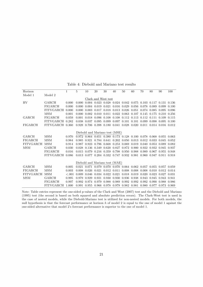
Table 4: Diebold and Mariano test results
Horizon 1 5 10 20 30 40 50 60 70 80 90 100Model 1 Model 2
Clark and West testHV GARCH 0.000 0.000 0.004 0.023 0.028 0.024 0.042 0.075 0.103 0.117 0.131 0.136
FIGARCH 0.000 0.000 0.004 0.019 0.021 0.016 0.029 0.056 0.078 0.089 0.099 0.100FITVGARCH 0.000 0.000 0.003 0.017 0.018 0.013 0.026 0.051 0.074 0.085 0.095 0.096MSM 0.001 0.000 0.002 0.010 0.011 0.022 0.063 0.107 0.145 0.175 0.210 0.256
GARCH FIGARCH 0.059 0.001 0.018 0.096 0.108 0.108 0.112 0.113 0.112 0.111 0.109 0.115FITVGARCH 0.282 0.038 0.037 0.095 0.099 0.097 0.101 0.101 0.099 0.098 0.095 0.100
FIGARCH FITVGARCH 0.360 0.928 0.706 0.398 0.180 0.041 0.028 0.020 0.011 0.014 0.016 0.012
Diebold and Mariano test (MSE)
GARCH MSM 0.970 0.972 0.864 0.651 0.380 0.173 0.128 0.100 0.078 0.068 0.055 0.063FIGARCH MSM 0.984 0.985 0.921 0.784 0.641 0.202 0.050 0.013 0.012 0.033 0.045 0.052FITVGARCH MSM 0.914 0.987 0.923 0.796 0.668 0.253 0.069 0.019 0.040 0.053 0.089 0.082MSM GARCH 0.030 0.028 0.136 0.349 0.620 0.827 0.872 0.900 0.922 0.932 0.945 0.937
FIGARCH 0.016 0.015 0.079 0.216 0.359 0.798 0.950 0.988 0.989 0.967 0.955 0.948FITVGARCH 0.086 0.013 0.077 0.204 0.332 0.747 0.932 0.981 0.960 0.947 0.911 0.918
Diebold and Mariano test (MAE)
GARCH MSM 0.005 0.021 0.071 0.079 0.070 0.070 0.064 0.062 0.057 0.055 0.057 0.059FIGARCH MSM 0.003 0.008 0.026 0.021 0.012 0.011 0.008 0.008 0.008 0.010 0.012 0.014FITVGARCH MSM <.001 0.009 0.046 0.034 0.022 0.021 0.018 0.019 0.020 0.023 0.027 0.031MSM GARCH 0.995 0.979 0.929 0.921 0.930 0.930 0.936 0.938 0.943 0.945 0.943 0.941
FIGARCH 0.997 0.992 0.974 0.979 0.988 0.989 0.992 0.992 0.992 0.990 0.988 0.986FITVGARCH 1.000 0.991 0.955 0.966 0.978 0.979 0.982 0.981 0.980 0.977 0.973 0.969
Note: Table entries represent the one-sided p-values of the Clark and West (2007) test and the Diebold and Mariano(1995) test (the second is based on both squared and absolute prediction errors). The Clark-West test is used inthe case of nested models, while the Diebold-Mariano test is utilized for non-nested models. For both models, thenull hypothesis is that the forecast performance at horizon h of model 2 is equal to the one of model 1 against theone-sided alternative that model 2’s forecast performance is superior to the one of model 1.
21

Table 5: Superior predictive ability (SPA) test results
Horizon Squared errors Absolute errorsHV GARCH FIGARCH MSM FITVGARCH HV GARCH FIGARCH MSM FITVGARCH
1 0 0.2 0.625 0.048 0.728 0.680 0.048 0.013 0.320 0.0055 0 0.003 1 0.015 0.113 0.535 0.048 0.033 0.465 0.02210 0 0.003 0.708 0.013 0.292 1 0.018 0.003 0.020 0.00520 0 0.02 0.480 0.06 0.520 1 0 0 0 030 0 0.003 0.590 0.308 0.870 1 0 0 0 040 0 0.003 0.223 0.823 0.335 1 0 0 0 050 0 0 0.010 1 0.050 1 0 0 0 060 0 0.003 0.010 1 0.058 1 0 0 0 070 0 0.003 0.015 1 0.090 1 0 0 0 080 0 0 0.037 0.95 0.098 1 0 0 0 090 0 0.007 0.030 1 0.095 1 0 0 0 0100 0 0.01 0.005 1 0.040 1 0 0 0 0
Note: The table entries represent the p-values of the SPA test of Hansen (2005) using two loss functions (MSE andMAE). The null hypothesis is that a particular model (benchmark model) cannot be outperformed by other candidatemodels. Each column shows the outcome of this test in terms of the one-sided p-ratios for the pertinent model againstall alternatives.
For the GARCH model, we find that it is inferior to alternative models
under MSE at all horizons but l=1. Interestingly, historical volatility is also
clearly out performed by some alternative forecasts so that the application of
our battery of time series models adds value in term of forecasting accuracy
under the MSE criterion. This is different under the MAE criterion where
the null of non-inferiority of HV for the alternative forecasts is never rejected.
If we would exclude HV from the competition, the SPA test would indicate
superiority of MSM compared to the GARCH type model at all forecast
horizons in line with the results of Tables 3 and 4. However, under the
MAE criterion, all our time series models would not add value to the naive
approach of using the in-sample average on a predictor for future volatility.
22

4 Conclusions
In the wake of the recent global financial crisis, a need has emerged for
a reconsideration of many facets of the existing financial system. Among
other developments, this has also led to a renewal of interest in Islamic fi-
nance. In essence, Islamic finance attempts to provide financial products
and instruments that are consistent with certain principles such as social re-
sponsibility, ethical and moral values and sustainability. Given the prevalent
interest in such products, we have investigated the statistical properties of
the Dow Jones Islamic Market World Index (DJIM), and have applied up-to-
date volatility models to model and forecast conditional volatility of DJIM
returns, accounting for both long memory and structural changes in the
volatility process, as well as the fact that volatility persistence may be due
to structural breaks. Given this, we use four different types of volatility mod-
els, namely, the Generalized Autoregressive Conditional Heteroskedasticity
(GARCH), Fractionally Integrated Generalized Autoregressive Conditional
Heteroskedasticity (FIGARCH), Fractionally Integrated Time Varying Gen-
eralized Autoregressive Conditional Heteroskedasticity (FITVGARCH) and
Markov-switching multifractal (MSM) models. While the GARCH model
serves as our benchmark volatility model, FIGARCH allows for long mem-
ory, FITVGARCH covers both long memory and structural breaks simulta-
neously, and the MSM model captures regime-switching that might lead to
spurious time-series characteristics close to ‘true’ long memory. The choice
of the DJIM is justified by the fact that it is the most widely used, most
comprehensive representative, and has the most adequate time series for the
Islamic stock market.
Our results show that the MSM model appears to be superior to other
models considered, especially at longer horizons, and with absolute errors
23

as loss criterion, for forecasting the volatility of the DJIM returns, and that
it outperforms the GARCH, FIGARCH and FITVGARCH for most of the
out-of-sample forecast comparison tests. However, this superiority against
GARCH-type models only has economic value under the MSE criterion,
while under the MAE loss function, all time-series models show predictive
capabilities that are inferior to historical volatility. Another finding is that
modeling the properties of long memory and time varying parameters in the
volatility process, as in the FITVGARCH model, can improve the forecast
performance for short and long forecasting horizons. Not surprisingly, the
classical GARCH model seems to be the worst performing model in terms
of forecasting future volatility among the models considered. All in all,
these results are not too different from those of other previous studies of the
comparative performance of volatility models: Calvet and Fisher (2004),
Lux(2008), Lux and Kaizoji (2007) and Lux, Morales-Arias and Satterhoff
(2013) all have found certain gains in forecastability of volatility with MSM
compared to GARCH-type models. The DJIM seems no exception and also
shows complete agreement with more traditional asset classes in terms of its
basic statistical features. This, however, casts doubt on whether investment
into the stocks represented in the DJIM could provide any safeguard against
extreme market gyrations like those observed over the last couple of years.
References
[1] Andersen TG Bollerslev T (1997) Heterogeneous information arrivalsand return volatility dynamics: uncovering the long-run in high fre-quency returns. Journal of Finance 52:975–1005.
[2] Andreou E, Ghysels E (2002) Detecting multiple breaks in financialmarket volatility dynamics. Journal of Applied Econometrics 17:579–600.
24

[3] Baillie RT, Bollerslev T, Mikkelsen H (1996) Fractionally integratedgeneralized autoregressive conditional heteroskedasticity. Journal ofEconometric 74:3–30
[4] Baillie RT, Morana C (2007) Modeling Long Memory and StructuralBreaks in Conditional Variances: an Adaptive FIGARCH Approach.ICER, Working Paper No. 11/2007.
[5] Beine M, Laurent S (2000) Structural change and long memory involatility: new evidence from daily exchange rates. Working paper, Uni-versity of Liege.
[6] Ben Nasr A, Boutahar M, Trabelsi A (2010) Fractionally integratedtime varying GARCH model. Statistical Methods and Applications19(3): 399-430.
[7] Bollerslev T (1986) Generalized autoregressive conditional het-eroskedasticity. Journal of Econometrics 31(3), 307–327
[8] Bollerslev T, Mikkelsen HO (1996) Modelling and pricing long memoryin stock market volatility. Journal of Econometrics 73:151–184
[9] Bos CS, Franses PH, Ooms M (1999) Long memory and level shifts:re-analyzing inflation rates. Empirical Economics 24,427–449
[10] Brockwell PJ, Dahlhaus R (2004) Generalized Levinson- Durbin andBurg algorithms. Journal of Econometrics 118(1-2), 129–149
[11] Calvet L, Fisher A (2001) Forecasting multifractal volatility, Journalof Econometrics 105, 27-58
[12] Calvet L, Fisher A (2004) Regime switching and the estimation of mul-tifractal processes, Journal of Financial Econometrics 2,49–83
[13] Clark T, West K (2007) Approximately normal tests for equal predictiveaccuracy in nested models, Journal of Econometrics 138,291–311
[14] Cont R (2001) Empirical Properties of Asset Returns: Stylized Factsand Statistical Issues. Quantitative Finance 1, 223-236
[15] Davidson JEH (2004) Conditional heteroskedasticity models and a newmodel. Journal of Business and Economic Statistics 22,16–29
[16] Diebold FX (1986) Comment on “ Modeling the persistence of condi-tional variance”. by Engle R, Bollerslev T. Econometric Reviews 5:51–56
[17] Diebold F X, Mariano R S (1995) Comparing predictive accuracy, Jour-nal of Business and Economic Statistics, 13(3), 253–263.
25

[18] Ding Z, Granger CWJ, Engle RF (1993) A long memory property ofstock market returns and a new model. Journal of Empirical Finance1:83–106
[19] Hammoudeh S, Jawadi F, Sarafrazi S (2013) Interactions betweenconventional and islamic stock markets: a hybrid threshold analysis.Mimeo, Drexel University, PA, U.S.A.
[20] Hansen, PR (2005). A test for superior predictive ability. Journal ofBusiness and Economic Statistics, 23, 365-380.
[21] Hill B (1975) A simple general approach to inference about the tail ofa distribution. The Annals of Statistics, 3(5), 1163-1174
[22] Leovey A, Lux T (2012) Parameter estimation and forecasting for mul-tiplicative log-normal cascades, Physical Review, E85, 046114
[23] Liu R, di Matteo T, and Lux T (2007) True and apparent scaling: Theproximities of the Markov-Switching Multifractal Model to long-rangedependence. Physica A, 383:35-42
[24] Lobato IN, Savin NE (1998) Real and spurious long memory propertiesof stock market data. Journal of Business and Economic Statistics,16:261-268
[25] Lux T (2008) The Markov-Switching Multifractal Model of asset re-turns: GMM estimation and linear forecasting of volatility. Journal ofBusiness and Economic Statistics, 26:194-210
[26] Lux T, Kaizoji T (2007) Forecasting volatility and volume in the Tokyostock market: Long memory, fractality and regime switching. Journalof Economic Dynamics and Control, 31:1808-1843
[27] Lux T, Morales-Arias L, Sattarhoff C (2013) Forecasting daily varia-tions of stock index returns with a multifractal model of realized volatil-ity. Working paper, University of Kiel
[28] Lamoureux CG, Lastrapes WD (1990) Persistence in variance, struc-tural change and the GARCH model. Journal of Business and Eco-nomic Statistics, 8:225–34
[29] Mandelbrot B, Fisher A, Calvet LE (1997) A multifractal model of assetreturns. Mimeo: Cowles Foundation for Research in Economics.
[30] Martens M, van Dijk D, de Pooter M (2004) Modeling and forecastingS&P 500 volatility: long memory, structural breaks and nonlinearity.Tinbergen Institute Discussion Paper 04-067/4.
26

[31] Morana C, Beltratti A (2004) Structural change and long-range depen-dence in volatility of exchange rates: either, neither or both? Journalof Empirical Finance, 11:629–658
[32] Rapach DE, Strauss, JK (2008) Structural breaks and GARCH modelsof exchange rate volatility. Journal of Applied Econometrics, 23(1): 65–90
[33] Rapach DE, Strauss, JK, Wohar, ME (2008) Forecasting stock returnvolatility in the presence of structural breaks. In Forecasting in thePresence of Structural Breaks and Model Uncertainty, David E. Ra-pach and Mark E. Wohar (Eds.), Vol. 3 of Frontiers of Economics andGlobalization, Bingley, United Kingdom, Emerald: 381–416
27