Forecasting skewness in stock returns: Evidence from firm ...

Forecasting Skewness in Stock Returns: Evidence from Firm-Level Data in Tokyo Markets∗

Mariko Fujii§♦ Makoto Takaoka§

July 2005

∗ This paper was presented at the 2005 Daiwa International Workshop on Financial Engineering, held on July 26 at Kyoto University. The research was conducted as part of a project at the Center for Japanese Economy and Business, Columbia University. Financial assistance from the Itoh Foundation USA is gratefully acknowledged. Please do not quote without the authors’ permission. § Research Center for Advanced Science and Technology, the University of Tokyo,

Komaba, Tokyo 153-8904, JAPAN ♦ Corresponding author. E-mail address: [email protected]

1

Abstract

Although it is well known that the market rate of return tends to show negative skewness, we find that the return distribution of individual stocks has shown positive skewness in the two principal Tokyo markets from 1980 to 2001. This is consistent with the results reported for the US market. Positive skewness in the returns is more evident for smaller firms.

From our analysis of pooled cross-section data of individual stocks from 1990 to 2001, we find that there is clear evidence of the predictive power in the information up until the current period for the skewness in the following period. Specifically, a higher volatility and skewness in the return distribution of the current period is followed by a higher value of skewness in the following period. Also, the up trends in own returns in the preceding periods may explain the rather negatively skewed return distribution in the following period.

Hong and Stein’s (2003) model predicts a relation between turnover and skewness. For 1990 to 2001, negative relation to the skewness has been found to hold for smaller cap firms with past de-trended turnover. Furthermore, after the regulatory change in short-selling enacted in February 2002, we find more supportive evidence that high trend-adjusted turnover predicts more negative skewness in returns. Overall, our empirical evidence suggests that conditional skewness is partly explained by previous de-trended trading proxies, however, the results are not conclusive for the data in Tokyo markets. Key words: firm-level stock returns, conditional skewness, volatility, Japanese stock market

2

Forecasting Skewness in Stock Returns: Evidence from Firm-Level Data in Tokyo Markets

1. Introduction In this paper, we first examine whether the return distribution of individual stocks in Tokyo’s two principal markets is described by log-normal distribution, as often modeled, and then investigate the mechanism to cause the asymmetry found in the return distribution with reference to the model of Hong and Stein (2003) of investor heterogeneity with institutional frictions. It may be possible that the distribution has either positive or negative third moments, as reported by the literature on the US capital markets. Although it is extensively reported that the market rate of return tends to show negative skewness, the return distribution of individual stocks in Tokyo markets has not yet been documented in detail to our knowledge. Duffee (1995) and Chen, Hong and Stein (2001, referred to as CHS (2001) hereafter) reported positive skewness of individual stock return distributions for the US market, and our data may exhibit similarities in firm-level stock returns distributions as well. We are also interested in the difference among firm-size groups.

As to the mechanism causing the asymmetric return distribution, there are competing hypotheses such as those based on leverage effects, a volatility feedback mechanism, and stochastic bubble. These studies mostly focus on asymmetric volatility and its relation to returns. Empirical findings are also extensively discussed in the literatures such as Beckaert and Wu (2000) both at firm- and market-level. With regard to more general aspects of asymmetry and other anomalous cross-sectional evidence in return distributions, the models which combine mild assumptions about investor irrationality with institutional frictions are offered.1 Among the belief-based models, Hong and Stein (2003) presented an interesting theoretical model of investor heterogeneity with institutional frictions. Their model predicts a relation between turnover and skewness. To be specific, their model predicts that markets may exhibit asymmetric return distributions in higher order conditional moments if some agents are short-sale constrained in their trading activity despite the existence of different opinions on the intrinsic value of stocks. Empirical work by CHS (2001) was done using US data based on this model. We examine their hypothesis in detail using the data from 1980 to 2001 in Tokyo markets.

Since we have a good opportunity in Japan to test the effects of a change of regulations on short-selling in stock trading, which was enacted in February 2002, we focus on the effects of tighter short-sale constraints as well. The results we obtained show that the institutional framework affects the return distribution and its conditional moments to some extent.

Our analysis of pooled cross-section data of individual stocks will show clear evidence of predictive power in the information preceding time for the skewness in period . Specifically, the greater the volatility and skewness in the current period, the greater the value of the skewness in the following period. Also, the up trends in own

t1t +

1These developments are surveyed in Barberis and Thaler (2003).

3

returns in the preceding periods may explain a rather negatively skewed return distribution in the following period. On the other hand, the effects of the trading variables as proxies for differences in opinion in the preceding period seem to be not so robust as such other variables as own skewness, volatility, and cumulative rate of return. Still, systematic relations to the skewness were evident in trading variables for small-cap firms in the 1990s through 2001.

Theoretical investigation as to why firm-level returns data show positive skewness and the underlying economic mechanism to explain this asymmetry is a great challenge for study. In reality, heterogeneity of agents inclusive of differences in preferences and information play an important role in ensuring active trades in the markets (Kandl and Pearson (1995)). From this viewpoint, the models of heterogeneous agents are attractive to explain asymmetries observed in the markets.

In the following sections, the patterns of the return distributions are carefully examined. Analysis to identify the causes bringing about the asymmetry in the firm-level return distribution is presented in Section 4, and robustness tests are in Section 5. A summary of the analysis and a future agenda for research conclude the paper. 2 Framework of Analysis 2.1 Definitions of the Variables This section defines the variables used in our analysis and explains the data source. Stock price data are the daily prices of the non-financial corporations listed on the first and second sections of the Tokyo Stock Exchange. These are Japan’s two principal exchanges in terms trading activity and number of listed stocks. Based on daily price data, individual stock returns are defined as excess return over that of the TOPIX market index. Using market-adjusted return allows us to focus on the factors associated with individual stocks. Specifically, the market-adjusted daily return of stock ,i iRτ , is defined as the log change in the stock price less the log change in the market index; daily returns for firm

at timei τ , iRτ , is calculated, using the stock price iPτ , as

1 1

log logii

i

P TOPIXRP TOPIX

ττ

τ τ− −

⎛ ⎞τ= −⎜⎝ ⎠

,⎟ (1)

where iPτ is the closing price of stock on i thτ day of the entire sample data sequence for firm . i For each firm i , data are sub-grouped according to six-month periods denoted by t . These are either April to September or October to March, to be consistent with the usual accounting periods for Japanese corporations. We also tested with the data sets consisting of January through June and July through December; almost similar results were obtained as those reported here. In later sections, we also use the groupings of three-month period and details will be explained in Section 5.2 and 5.3.

4

2.2 Measure of Skewness To measure the skewness of the return distribution, two alternative variables and are defined, following research by CHS (2001).

itSKEW

itDUVOL 2 is the degree of the skewness of daily stock returns for the firm measured over the six-month period . Specifically, is calculated by taking the sample third moment of daily returns, and dividing it by the sample standard deviation of daily returns raised to the third power. Thus, for any stock over any six-month period t , we have

and as;

itSKEWi

t itSKEW

itSIGMAi

itSIGMA itSKEW

( )1

1 22

1

11

it

it

S

itit ill Sit

SIGMA R Rn−

/

= +

⎧ ⎫⎪ ⎪= −⎨ −⎪ ⎪⎩ ⎭∑ ,⎬ (2)

( ) ( )1

3 3

1( 1)( 2)

it

it

Sit

itit il itl Sit it

nSKEW R SIGMARn n−= +

= − /− − ∑ , (3)

where is the number of observations of itn iRτ during the period , is ,

and

t itS1

tijj

n=∑

itR is 1

11

it

it it

Siln l S

R−= +∑ , which is the mean return for stock during the period .

A positive value of corresponds to a distribution skewed to the right.

i t

itSKEWThe second variable to measure the asymmetry of stock returns is

which is the up-to-down variance ratio. This is computed as follows: for any stock over any six-month period , we divide our samples into two sub-groups, one with returns below the period mean (’down’ days) and those with returns above the period mean (’up’ days), and compute the standard deviation for each of these sub-samples separately. We then take the log of the ratio of the standard deviation on the up days to the standard deviation on the down days. Accordingly, we have

itDUVOLi

t

1

1

21

21

( 1) ( ) ( )log

( 1) ( ) ( )

it

it

it

it

Sdit itit il ill S

it Suit itit il ill S

n R I RR RDUVOL

n R IR R−

−

= +

= +R

⎧ ⎫− − ⋅ −⎪ ⎪= ⎨ ⎬− − ⋅ −⎪ ⎪⎩ ⎭

∑∑

(4)

where ( )I X is an index function as

1 0

( )0 0

XI X

X>⎧

= ,⎨ ≤⎩

and the number of up and down days, andUn Dn , are defined as

1 1( )it

it

Suitit ill S

n I R R−= +

= −∑ and 1 1

(it

it

Sditit ill S

n I R−= +

= )R−∑ respectively.

A higher value of means that daily returns are more positively skewed, corresponding to a more right-skewed distribution. Because we only use the second

itDUVOL

2In CHS (2001), , is defined as the negative of as defined in this paper. NCSKEW SKEW

5

moment of the returns when we calculate , the variable is less affected by outliers in the sample than .

itDUVOL itDUVOL

itSKEWTo check the impact caused by outliers, we also calculate and

as follows; itDMA itDOUT

itit itDMA MEDIANR= − , (5) where MEDIAN refers to the sample median of the return distribution and itR is defined as above. measures how the return distribution is shaped asymmetrically. On the other hand, if the shape of the distribution is affected by small numbers of large outliers, this possibility should be captured by , which is calculated by counting the number of outliers. Outliers are defined as data with values exceeding three times the sample standard deviation, . Namely,

itDMA

itDOUT

3 itSIGMA

1 1

( ( 3 ) ( 3 ))it

it

S

it itit il it il it itl S

DOUT I R SIGMA I R SIGMA nR R−= +

= − − − − −∑ / (6)

where ( )I X is an index function. Since and are more sensitively affected by the number of outliers, a large positive value of corresponds to having more observations in the right end of the distribution.

itDMA itDOUT

itDOUT

In calculating the above variables, we drop any six-month period from the data set if stock has more than six missing observations of daily returns.

ti 3

2.3 Cumulative Returns and Trading Volume We also define four variables to represent the trading volume of each stock. These are important regressors as a proxy for differences of opinion in the analysis to be conducted in the following sections. is defined as the ratio of the average monthly trading volume to the number of shares outstanding for firm . is derived by subtracting the value of an 18-month moving average of , namely,

itTURNOVERi itDTURNOVER

itTURNOVER

1 1

16

it

it

Sim

itm S im

tradeTURNOVERtotal

−= +

= ∑ (7)

where itradeτ is the number of shares traded of stock on the i thτ day, itotal τ is the number of shares outstanding of stock in the i thτ day.

1 1

1 it

it

S

it imm Sit

TRADE traden

−= +

= ,∑ (8)

3For small firms, there sometimes are no trades. This survivorship bias is inevitable in obtaining homogeneous samples to calculate the statistics of return distribution.

6

2

0

13it it i t k

k

DTURNOVER TURNOVER TURNOVER , −=

= − ∑ . (9)

It is possible for to be biased because of specific characteristics of

a firm’s share owner structure, so, alternatively, we define to capture the detrended trading activities for the firm in period as follows;

TURNOVERitDTRADE

i t

213 0it i t kk

itit

TRADE TRADEDTRADE

TRADE, −=

−= .∑

(10)

In the theoretical model of Hong and Stein (2003), the trading variables are expected to capture the size of differences of opinions.

The market-adjusted cumulative return in period , t itRET , is defined as;

1 1

it

it

S

it imm S

RET R−= +

= .∑

That is, itRET represents the sequence of daily returns, which is the de-meaned excess return relative to the TOPIX for stock , in either six-month or three-month period . i t 3 Data and Stock Return Distribution in Tokyo Markets 3.1 Data All the data on stock prices and trading volume are from the Tokyo Stock Exchange (TSE) daily data summary. Unless otherwise specified, samples are non-financial corporations listed on either the TSE’s first or second section. The data period is April 1, 1980 to March 31, 2002. This is 5,736 trading days. The total number of available listed firms is 1,741.

In our regression with firm-level data, we use non-overlapping observations of either six-months or three-months. A maximum of five missing daily observations is allowed. The sub periods start in April or October, but this does not affect the results in general.4 However, the choice of a time horizon for measuring skewness may affect the regression results and this point will be discussed in Section 5.2.

Earlier research on US markets found that firm size affects the return distribution. Thus, we define the variable for firm i in period t as a log of the value of the total market capitalization of the firm measured in million yen.

itLOGSIZE5 Return data are

disaggregated by firm size. The available data are sorted according to firms’ current total capitalization in each period. This listing is divided into quintiles with group 5 containing the largest stocks. 4In Section 5.3, a three-month sub-period starting in March is used because of the timing of the regulatory change occurred in February 2002. 5The total market capitalization of each firm is based on the end-day of each accounting period. Data are from Toyokeizai Data Disk 2001.

7

3.2 Characteristics of Firm-level Return Data A variety of summary statistics for our sample are presented in Tables 1 and 2. The means and standard deviations of all of our variables for the full sample of individual firms, five size-based sub samples, and the market as a whole, represented by TOPIX defined as the value-weighted index of the Tokyo Stock Exchange, are shown for two periods: 1980-89 and 1990-2001. Contemporaneous correlation and autocorrelation among these variables are calculated and summarized in the Appendix Table. The period of the asset price bubbles in the late 1980s deserves special attention. For this reason, we divided the sample period into two segments; the period including the peak of the bubble, which was the end of 1989, and the period after the bubble. In Tables 1 and 2, positive skewness is observed for any size individual firm and the mean value of for all firms is SKEW 0 484. for 1980 to 1989, and for 1990 to 2001. In general, smaller firms (first quintile) exhibit a more positively skewed return distribution. In other words, larger firms show relatively symmetric return distributions and are described better as normal distributions. This observation applies to the data in both data periods. Returns were more skewed in the 1980s than in 1990 to 2001. This may be related to the behavior of the market index, which showed a sharp rise in the late 1980s. Indeed, the

0 249.

RET was generally much higher in the 1980s. Asymmetries measured by are confirmed by calculated values of SKEWDUVOL . Smaller firms and data in the 1980s show higher values of DUVOL , being associated with positively skewed distribution of returns.6 These asymmetries are closely associated with higher values of DOUT , rather than higher values of , implying that outliers matter in the creation of a skewed distributions. By any statistics calculated in this paper, asymmetries of the return distribution are more evident for smaller firms. For the US data, CHS (2001) have reported more positively skewed distributions for small-cap firms as well, which suggest that this asymmetry may be caused by more arbitrary disclosure of good information on their own firms. Regarding the information structure, it might be true that managers of smaller firms have more scope for managerial discretion in disclosure, implying that bad news may not be released immediately. This hypothesis could be applied to Japanese case as well. However, disclosure rules are not a function of firm size, so smaller firms are as obligated as larger ones to disclosure. Given the trend toward stricter application of these rules, there remain questions about this explanation even for the 1990s.

DMA

Smaller firms seem to be more volatile than larger ones. is larger for smaller firms and this is true for both sub-periods. Stock volatility, particularly when measured in TOPIX, looks slightly higher in the 1990s and later.

itSIGMA

iRτ

6Under the hypothesis that daily return in period follows an identical normal distribution

independently, follows

t

224 ( 2)( 3)

( 1) ( 3)( 5)(0 )it it

it it it

n n nn n n

N − −

+ + +,itSKEW . When we test the samples with this

hypothesis, 5,236 samples among 8,067 for 1980 to 1989 data and 7,799 among 17,670 are rejected against the null hypothesis at a 5 percent significance level.

8

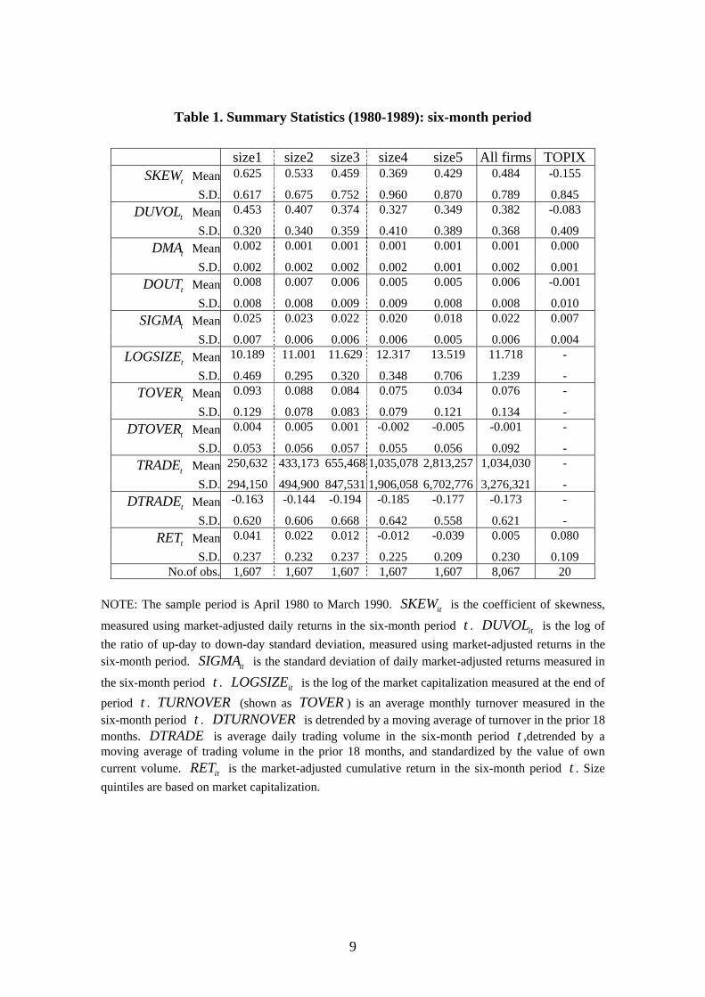
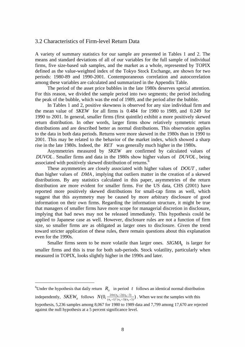
Table 1. Summary Statistics (1980-1989): six-month period

size1 size2 size3 size4 size5 All firms TOPIX tSKEW Mean 0.625 0.533 0.459 0.369 0.429 0.484 -0.155

S.D. 0.617 0.675 0.752 0.960 0.870 0.789 0.845

tDUVOL Mean 0.453 0.407 0.374 0.327 0.349 0.382 -0.083

S.D. 0.320 0.340 0.359 0.410 0.389 0.368 0.409

tDMA Mean 0.002 0.001 0.001 0.001 0.001 0.001 0.000

S.D. 0.002 0.002 0.002 0.002 0.001 0.002 0.001

tDOUT Mean 0.008 0.007 0.006 0.005 0.005 0.006 -0.001

S.D. 0.008 0.008 0.009 0.009 0.008 0.008 0.010

tSIGMA Mean 0.025 0.023 0.022 0.020 0.018 0.022 0.007

S.D. 0.007 0.006 0.006 0.006 0.005 0.006 0.004

tLOGSIZE Mean 10.189 11.001 11.629 12.317 13.519 11.718 -

S.D. 0.469 0.295 0.320 0.348 0.706 1.239 -

tTOVER Mean 0.093 0.088 0.084 0.075 0.034 0.076 -

S.D. 0.129 0.078 0.083 0.079 0.121 0.134 -

tDTOVER Mean 0.004 0.005 0.001 -0.002 -0.005 -0.001 -

S.D. 0.053 0.056 0.057 0.055 0.056 0.092 -

tTRADE Mean 250,632 433,173 655,468 1,035,078 2,813,257 1,034,030 -

S.D. 294,150 494,900 847,531 1,906,058 6,702,776 3,276,321 -

tDTRADE Mean -0.163 -0.144 -0.194 -0.185 -0.177 -0.173 -

S.D. 0.620 0.606 0.668 0.642 0.558 0.621 -

tRET Mean 0.041 0.022 0.012 -0.012 -0.039 0.005 0.080

S.D. 0.237 0.232 0.237 0.225 0.209 0.230 0.109 No.of obs. 1,607 1,607 1,607 1,607 1,607 8,067 20

NOTE: The sample period is April 1980 to March 1990. is the coefficient of skewness,

measured using market-adjusted daily returns in the six-month period . is the log of the ratio of up-day to down-day standard deviation, measured using market-adjusted returns in the six-month period. is the standard deviation of daily market-adjusted returns measured in

the six-month period . is the log of the market capitalization measured at the end of period . (shown as T ) is an average monthly turnover measured in the six-month period .

itSKEWt itDUVOL

itSIGMAt itLOGSIZE

t TURNOVER OVERt DTURNOVER is detrended by a moving average of turnover in the prior 18

months. is average daily trading volume in the six-month period ,detrended by a moving average of trading volume in the prior 18 months, and standardized by the value of own current volume.

DTRADE t

itRET is the market-adjusted cumulative return in the six-month period . Size quintiles are based on market capitalization.

t

9

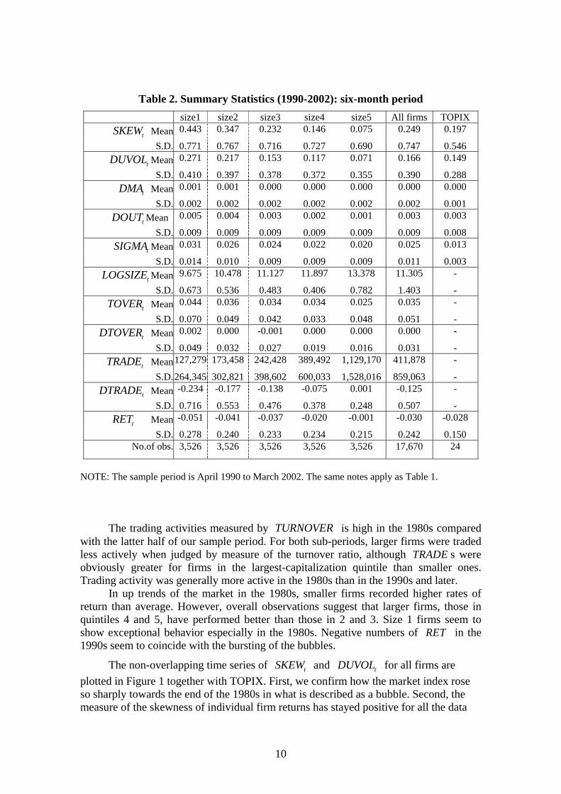
Table 2. Summary Statistics (1990-2002): six-month period size1 size2 size3 size4 size5 All firms TOPIX

tSKEW Mean 0.443 0.347 0.232 0.146 0.075 0.249 0.197

S.D. 0.771 0.767 0.716 0.727 0.690 0.747 0.546

tDUVOL Mean 0.271 0.217 0.153 0.117 0.071 0.166 0.149

S.D. 0.410 0.397 0.378 0.372 0.355 0.390 0.288 Mean tDMA 0.001 0.001 0.000 0.000 0.000 0.000 0.000

S.D. 0.002 0.002 0.002 0.002 0.002 0.002 0.001

tDOUT Mean 0.005 0.004 0.003 0.002 0.001 0.003 0.003

S.D. 0.009 0.009 0.009 0.009 0.009 0.009 0.008

tSIGMA Mean 0.031 0.026 0.024 0.022 0.020 0.025 0.013

S.D. 0.014 0.010 0.009 0.009 0.009 0.011 0.003

tLOGSIZE Mean 9.675 10.478 11.127 11.897 13.378 11.305 -

S.D. 0.673 0.536 0.483 0.406 0.782 1.403 -

tTOVER Mean 0.044 0.036 0.034 0.034 0.025 0.035 -

S.D. 0.070 0.049 0.042 0.033 0.048 0.051 -

tDTOVER Mean 0.002 0.000 -0.001 0.000 0.000 0.000 -

S.D. 0.049 0.032 0.027 0.019 0.016 0.031 - MeantTRADE 127,279 173,458 242,428 389,492 1,129,170 411,878 -

S.D.264,345 302,821 398,602 600,033 1,528,016 859,063 - Mean tDTRADE -0.234 -0.177 -0.138 -0.075 0.001 -0.125 -

S.D. 0.716 0.553 0.476 0.378 0.248 0.507 - tRET Mean -0.051 -0.041 -0.037 -0.020 -0.001 -0.030 -0.028

S.D. 0.278 0.240 0.233 0.234 0.215 0.242 0.150 No.of obs. 3,526 3,526 3,526 3,526 3,526 17,670 24

NOTE: The sample period is April 1990 to March 2002. The same notes apply as Table 1.

The trading activities measured by is high in the 1980s compared

with the latter half of our sample period. For both sub-periods, larger firms were traded less actively when judged by measure of the turnover ratio, although s were obviously greater for firms in the largest-capitalization quintile than smaller ones. Trading activity was generally more active in the 1980s than in the 1990s and later.

TURNOVER

TRADE

In up trends of the market in the 1980s, smaller firms recorded higher rates of return than average. However, overall observations suggest that larger firms, those in quintiles 4 and 5, have performed better than those in 2 and 3. Size 1 firms seem to show exceptional behavior especially in the 1980s. Negative numbers of RET in the 1990s seem to coincide with the bursting of the bubbles.

The non-overlapping time series of and for all firms are plotted in Figure 1 together with TOPIX. First, we confirm how the market index rose so sharply towards the end of the 1980s in what is described as a bubble. Second, the measure of the skewness of individual firm returns has stayed positive for all the data

tSKEW tDUVOL

10

period, although some fluctuations in values are observed. Third, and show almost the same pattern. Thus, for regression analysis, we only use

as the measure of skewness in the return distribution.

itSKEW

itDUVOL

itSKEW

Figure 1. , SKEW DUVOL and TOPIX: 1980 to 2001

-0.5

0

0.5

1

1.5

2

1980-1st

1981-1st

1982-1st

1983-1st

1984-1st

1985-1st

1986-1st

1987-1st

1988-1st

1989-1st

1990-1st

1991-1st

1992-1st

1993-1st

1994-1st

1995-1st

1996-1st

1997-1st

1998-1st

1999-1st

2000-1st

2001-1st

0

500

1000

1500

2000

2500

3000

SKEW

DUVO L

TO PIX

From the panels in the Appendix, some hints are obtained regarding the relationships among variables. Panel A of the Appendix Table shows the contemporaneous correlation between any pair of the variables and Panel B shows the lagged correlation among the variables. It is worth noting that has a strong positive correlation with

SKEWDUVOL , whose correlation coefficient is . This

suggests that these two variables represent very similar pieces of information despite their totally different means of derivation. On the other hand, their correlations with

are relatively weak, as

0 874.

SIGMA 0 092. and 0 159. , respectively. Thus, to predict the variables to measure the skewness of the return distribution is not necessarily to provide any information about the variance.

Autocorrelation is rather small: 0.136 for and 0SKEW 190. for DUVOL . For , it is , suggesting that that and SIGMA 0 611. SKEW DUVOL are not persistent

although appears relatively persistent. The correlation between SIGMA tRET and is . Between tSIGMA 0 099− . tRET and 1tSIGMA + it is 0 202− . . This implies that a

decrease in stock return tends to slightly increase volatility contemporaneously and in the following period. 3.3 Market Returns: TOPIX Most previous researchers report that market returns are negatively skewed, while our statistics for individual stocks have shown a positive skewness. These statistics imply

11

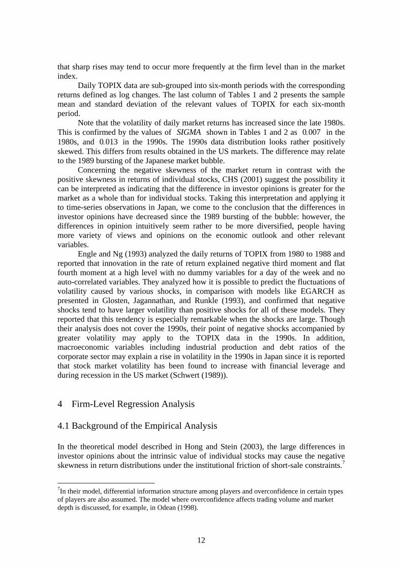
that sharp rises may tend to occur more frequently at the firm level than in the market index. Daily TOPIX data are sub-grouped into six-month periods with the corresponding returns defined as log changes. The last column of Tables 1 and 2 presents the sample mean and standard deviation of the relevant values of TOPIX for each six-month period. Note that the volatility of daily market returns has increased since the late 1980s. This is confirmed by the values of shown in Tables 1 and 2 as in the 1980s, and in the 1990s. The 1990s data distribution looks rather positively skewed. This differs from results obtained in the US markets. The difference may relate to the 1989 bursting of the Japanese market bubble.

SIGMA 0 007.0 013.

Concerning the negative skewness of the market return in contrast with the positive skewness in returns of individual stocks, CHS (2001) suggest the possibility it can be interpreted as indicating that the difference in investor opinions is greater for the market as a whole than for individual stocks. Taking this interpretation and applying it to time-series observations in Japan, we come to the conclusion that the differences in investor opinions have decreased since the 1989 bursting of the bubble: however, the differences in opinion intuitively seem rather to be more diversified, people having more variety of views and opinions on the economic outlook and other relevant variables. Engle and Ng (1993) analyzed the daily returns of TOPIX from 1980 to 1988 and reported that innovation in the rate of return explained negative third moment and flat fourth moment at a high level with no dummy variables for a day of the week and no auto-correlated variables. They analyzed how it is possible to predict the fluctuations of volatility caused by various shocks, in comparison with models like EGARCH as presented in Glosten, Jagannathan, and Runkle (1993), and confirmed that negative shocks tend to have larger volatility than positive shocks for all of these models. They reported that this tendency is especially remarkable when the shocks are large. Though their analysis does not cover the 1990s, their point of negative shocks accompanied by greater volatility may apply to the TOPIX data in the 1990s. In addition, macroeconomic variables including industrial production and debt ratios of the corporate sector may explain a rise in volatility in the 1990s in Japan since it is reported that stock market volatility has been found to increase with financial leverage and during recession in the US market (Schwert (1989)). 4 Firm-Level Regression Analysis 4.1 Background of the Empirical Analysis In the theoretical model described in Hong and Stein (2003), the large differences in investor opinions about the intrinsic value of individual stocks may cause the negative skewness in return distributions under the institutional friction of short-sale constraints.7

7In their model, differential information structure among players and overconfidence in certain types of players are also assumed. The model where overconfidence affects trading volume and market depth is discussed, for example, in Odean (1998).

12

Chen, Hong and Stein (2001) have shown one way to verify this hypothesis by regression analysis using data on returns and trading volume for all NYSE and AMEX firms. In the Hong-Stein model, large differences in investor opinions are associated with a larger amount of trading. However, if the more-bearish investors face short-selling constraints, part of their sales demand is hidden in the current period and their hidden demand is revealed in the following period. This causes a sharp drop in price and makes the skewness of the rate of return distribution negative in the subsequent period. The Hong-Stein model is consistent with the view that the efficiency of the market is assured by the assumption of there being rational and risk-neutral arbitragers while investors facing constraints on short-selling are present. Further, the relation between the third moment of the rate of return and trading volume can be analyzed without any constraint on the sign of skewness in the rate of return.

Based on this hypothesis, CHS (2001) reported that negative skewness occurs most often in two cases. First, the trading volume in the previous six-month period is large compared to the preceding trend, and, second, the rate of return in the preceding 36 months is positive (that is, stocks are in some situation like a bubble). In this section, we conduct a similar regression analysis to identify the variables to determine the features of the return distribution using firm-level data. The purpose is to show whether any variables have forecasting power regarding the third moment in the return distribution in the following period. The variables used for regressions are as defined in section 2 and individual stock data are from April 1980 to March 2002. For the analysis, the following model is assumed:

1 0 1 2 3

4 8 4 1

it it it it

it it it

SKEW SIGMA DTURNOVER LOGSIZERET RET

α α α αα α ε

+

− +

= + + ++ + + +L

where itε is an error term. To consider possible heteroskedasticity and autocorrelations in error terms, adjusted t-values are calculated.8 can be replaced by

in the alternative specification. itDTURNOVER

itDTRADE 4.2 Pooled Regression: Cross-section of all firms First, we regressed against , , and preceding cumulative returns of firm to examine how the conditional third moment of the rate of return at is accounted for with information until time . In addition to the regressors described so far, we also include six-month period dummy variables to control period-specific macroeconomic conditions and the variable as explanatory variables.

1i tSKEW , + itSKEW itSIGMA itDTURNOVERi

1t + t

itLOGSIZE

Table 3 presents the results of the pooled cross-section regression of all firms. The regression period is divided into the first 10 years, which is before the bubble burst, and the subsequent 12 years. In both periods, all the coefficients except some lagged variables of cumulative returns are estimated with statistical significance at the 5 percent level.

8Based on these adjusted t-values, adjusted p-values are reported in the following tables.

13

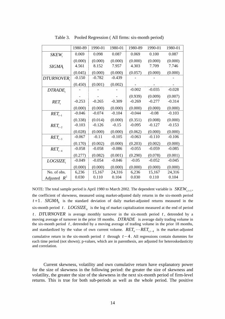
Table 3. Pooled Regression ( All firms: six-month period)

1980-89 1990-01 1980-01 1980-89 1990-01 1980-01

tSKEW 0.069 0.098 0.087 0.069 0.100 0.087 (0.000) (0.000) (0.000) (0.000) (0.000) (0.000)

tSIGMA 4.561 8.152 7.957 4.303 7.709 7.746 (0.045) (0.000) (0.000) (0.057) (0.000) (0.000)

tDTURNOVER -0.150 -0.782 -0.439 - - - (0.450) (0.001) (0.002) - - -

tDTRADE - - - -0.002 -0.035 -0.028 - - - (0.939) (0.009) (0.007)

tRET -0.253 -0.265 -0.309 -0.269 -0.277 -0.314 (0.000) (0.000) (0.000) (0.000) (0.000) (0.000)

1tRET − -0.046 -0.074 -0.104 -0.044 -0.08 -0.103 (0.338) (0.014) (0.000) (0.351) (0.008) (0.000)

2tRET − -0.103 -0.126 -0.15 -0.095 -0.127 -0.153 (0.028) (0.000) (0.000) (0.062) (0.000) (0.000)

3tRET − -0.067 -0.11 -0.105 -0.063 -0.110 -0.106 (0.170) (0.002) (0.000) (0.203) (0.002) (0.000)

4tRET − -0.058 -0.058 -0.086 -0.055 -0.059 -0.085 (0.277) (0.082) (0.001) (0.290) (0.078) (0.001)

tLOGSIZE -0.049 -0.054 -0.046 -0.05 -0.052 -0.045 (0.000) (0.000) (0.000) (0.000) (0.000) (0.000)

No. of obs. 6,236 15,167 24,316 6,236 15,167 24,316 Adjusted 2R 0.030 0.110 0.104 0.030 0.110 0.104

NOTE: The total sample period is April 1980 to March 2002. The dependent variable is 1i tSKEW , + , the coefficient of skewness, measured using market-adjusted daily returns in the six-month period

. is the standard deviation of daily market-adjusted returns measured in the

six-month period . is the log of market capitalization measured at the end of period

.

1t + itSIGMAt itLOGSIZE

t DTURNOVER is average monthly turnover in the six-month period , detrended by a moving average of turnover in the prior 18 months. is average daily trading volume in the six-month period , detrended by a moving average of trading volume in the prior 18 months, and standardized by the value of own current volume.

tDTRADE

t4it i tRET RET , −L is the market-adjusted

cumulative return in the six-month period through t 4t − . All regressions contain dummies for each time period (not shown); p-values, which are in parenthesis, are adjusted for heteroskedasticity and correlation.

Current skewness, volatility and own cumulative return have explanatory power for the size of skewness in the following period: the greater the size of skewness and volatility, the greater the size of the skewness in the next six-month period of firm-level returns. This is true for both sub-periods as well as the whole period. The positive

14

coefficients of and indicate that the rate of return after high volatility and skewness tends to show larger positive skewness.

itSIGMA itSKEW

When trading volume is high relative to the previous trend, we observe a more negatively skewed distribution of daily returns in the next six-month period if the model is fitted to 1990 to 2001 data. The coefficients of DTURNOVER are

, and 0 150(1980 89)− . − 0 782(1990 2001)− . − 0 439(1980 2001)− . − , of which the coefficient for 1980 to 89 is statistically insignificant. This suggests that in periods after larger-than-trend trading volumes 1i tSKEW , + tends to be smaller, implying that the distribution in rate of return of period 1t + is skewed more to the left. Similar results are confirmed when we regress with the variable . The estimated coefficients are , , and

DTRADE0 002(1980 89)− . − 0 035(1990 2001)− . − 0 028(1980 2001)− . − . Again, the

coefficient for 1980 to 1989 turns out to be statistically insignificant. The result that all the coefficients of previous (accumulated rate of) returns are

negative and statistically significant indicates that stocks whose prices have been rising tend to have smaller s. This means the rates of return tend to be more negatively skewed. Total market capitalization is a factor in explaining the negative skewness in the following period. Estimated values are

SKEW

0 049(1980 89)− . − , 0 054(1990 2001)− . − , and in the specification with 0 046(1980 2001)− . − DTURNOVER .

It is noted that the statistical significance of these coefficients is strongly confirmed when the model is applied to the period 1990 to 2001 for both specifications. Also, the sizes of the coefficients are larger in the period after the bubble. Because the bubble period is more definitively characterized in its up trends than in its crash phase, it is not surprising that the model would not be fitted to these extraordinary situations. Thus, we will focus on the data for 1990 to 2001 that is the period after the crash of the bubble hereafter.

Another reason to focus on the data from 1990 to 2001 is related to the institutional framework. In Japanese capital markets, many deregulatory measures were taken in the 1990s. Among others, the full deregulation of brokerage fees in 1999 might have some impact on trading behavior.9 In later part of this paper, we examine more recent data and ask how empirical results are affected. 4.3 Cuts on Market Capitalization Next, we conduct regression analysis according to market-capitalization quintile. Comparing the features of each group, the larger stocks tend to have smaller skewness in their returns (the absolute value of is smaller), as shown in Tables 1 and 2. SKEW

Regression results are shown in panels A and B of Table 4. From the panels, we first confirm the stability of the estimated coefficients for and with positive sign. The explanatory power of past cumulative returns is, in general, negative in sign and is statistically significant at the 1 percent level for all the cases for up to one-period lag. However, the effects of longer lags are mixed. Lags of three periods or longer of are insignificant for almost all the cases, so such variables are deleted.

itSKEW itSIGMA

RETit

9Theoretical models typically assume that transaction costs are zero.

15

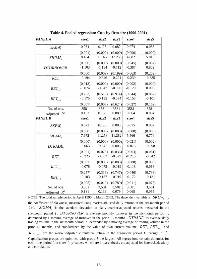
Table 4. Pooled regression: Cuts by firm size (1990-2001) PANEL A size1 size2 size3 size4 size5

tSKEW 0.064 0.125 0.082 0.074 0.088 (0.001) (0.000) (0.000) (0.000) (0.000)

tSIGMA 8.464 11.927 12.255 4.882 5.810 (0.000) (0.000) (0.000) (0.045) (0.007)

tDTURNOVER -1.103 -1.184 -0.712 -0.387 0.802 (0.000) (0.009) (0.199) (0.663) (0.202)

tRET -0.194 -0.346 -0.291 -0.239 -0.385 (0.013) (0.000) (0.000) (0.002) (0.000)

1tRET − -0.074 -0.047 -0.006 -0.120 0.009 (0.283) (0.518) (0.914) (0.044) (0.867)

2tRET − -0.175 -0.195 -0.034 -0.153 -0.101 (0.007) (0.006) (0.624) (0.027) (0.162)

No. of obs. 3581 3581 3581 3581 3581 Adjusted 2R 0.132 0.135 0.080 0.064 0.054

PANEL B size1 size2 size3 size4 size5

tSKEW 0.072 0.128 0.083 0.075 0.087 (0.000) (0.000) (0.000) (0.000) (0.000)

tSIGMA 7.672 11.258 11.282 5.566 6.776 (0.000) (0.000) (0.000) (0.021) (0.002)

tDTRADE -0.065 -0.041 0.006 -0.075 -0.098 (0.001) (0.078) (0.836) (0.063) (0.061)

tRET -0.225 -0.383 -0.329 -0.215 -0.342 (0.002) (0.000) (0.000) (0.008) (0.000)

1tRET − -0.078 -0.072 -0.019 -0.118 0.018 (0.257) (0.319) (0.747) (0.046) (0.738)

2tRET − -0.183 -0.187 -0.019 -0.172 -0.131 (0.005) (0.010) (0.789) (0.011) (0.075)

No. of obs. 3,581 3,581 3,581 3,581 3,581 Adjusted 2R 0.131 0.133 0.079 0.065 0.055



six-month period .

1t + itSIGMAt DTURNOVER is average monthly turnover in the six-month period ,

detrended by a moving average of turnover in the prior 18 months. is average daily trading volume in the six-month period , detrended by a moving average of trading volume in the prior 18 months, and standardized by the value of own current volume.

tDTRADE

t1it i tRET RET , −, and

2i tRET , − are the market-adjusted cumulative return in the six-month period t through . Capitalization groups are quintiles, with group 5 the largest. All regressions contain dummies for each time period (not shown); p-values, which are in parenthesis, are adjusted for heteroskedasticity and correlation.

2t −

16

Negative coefficients are estimated for DTURNOVER for two smaller

capitalization groups that are significant, but coefficients are not significant for large-cap groups. The variable turns out to be statistically significant with negative sign except for group 3. As an overall evaluation, the proposed model appears to be better fitted to smaller-cap groups by using either trading variable. Since CHS (2001) report that the coefficients on

itDTRADE

DTURNOVER are robust for large firms, the results with Japanese data are in contrast in this respect. This point will be discussed in the next subsection. 4.4 Why Do Smaller-Cap Firms Better Fit the Model? In the theoretical model of Hong and Stein (2003), skewness in stock returns is due to institutional frictions and differences of opinions. The previous subsection shows that small-cap firms appear to be better-explained by the model than larger-cap firms. Let us consider why. Differential trading regulations is not a reason because the same rules apply regardless of market capitalization.

Holding structure is a possible explanation. Data are in Table 5. First, the percentage of shares held by mutual fund increases as market-cap becomes larger. Because larger-cap firms show less-skewed distributions, mutual fund holdings are not a major factor in skewness in Tokyo markets. Second, the percentage of shares held by non-residents and financial institutions becomes higher as capitalization size increases. Investors such as non-residents and financial institutions may include hedge funds and other institutional investors, and it is presumed that large-cap stocks are subject to highly active trading.

On the other hand, for small-cap stocks, the percentage of shares held by non-financial corporations and the largest shareholders, which often includes the founders of a firm and is defined as the 10 largest holders, is high. Their trading may be rather infrequent. Small shareholders hold a relatively large share of small-cap stocks.10 A high percentage of shares being in the hands of non-financial corporations, largest shareowners, and smaller shareholders all imply less liquidity. Under such conditions, the trading impact may be relatively larger in small-caps than larger-cap stocks. And, if more conservative investors are involved in small stocks, an asymmetric pattern with positive skewness may arise because of their investment style.

When the share ownership structure described above is considered, we prefer the variable to DTRADE DTURNOVER as a de-trended trading proxies. Based on the regression results of the specification with , our tentative conjecture is that small-cap firms involve more conservative investors with relatively high trading costs, and thus the demand from bearish investors is more inclined to be hidden to create a negative relationship between conditional skewness and past turnover despite the positivity of observed skewness, given Hong and Stein (2003) as an underlying economic model. However, further testing this question is obviously needed.

DTRADE

10Small holders are those owning fewer than 50 trading units. The usual trading unit is 1,000 shares.

17

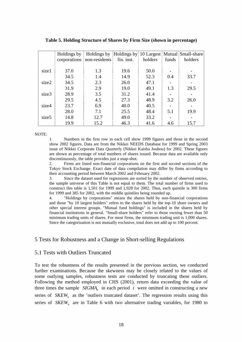
Table 5. Holding Structure of Shares by Firm Size (shown in percentage)

Holdings by corporations

Holdings by non-residents

Holdings byfin. inst.

10 Largest holders

Mutual funds

Small-share holders

size1 37.0 1.3 19.6 50.0 - - 34.5 1.4 14.9 52.3 0.4 33.7

size2 34.5 2.3 26.0 47.1 - - 31.9 2.9 19.0 49.1 1.3 29.5

size3 28.9 3.5 31.2 41.4 - - 29.5 4.5 27.3 48.9 3.2 26.0

size4 23.7 6.9 40.0 40.5 - - 28.0 7.1 25.5 48.4 5.1 19.9

size5 14.8 12.7 49.0 33.2 - - 19.9 15.2 46.3 41.6 4.6 15.7

NOTE:

1. Numbers in the first row in each cell show 1999 figures and those in the second show 2002 figures. Data are from the Nikkei NEEDS Database for 1999 and Spring 2003 issue of Nikkei Corporate Data Quarterly (Nikkei Kaisha Jouhou) for 2002. These figures are shown as percentage of total numbers of shares issued. Because data are available only discontinuously, the table provides just a snap-shot. 2. Firms are listed non-financial corporations on the first and second sections of the Tokyo Stock Exchange. Exact date of data compilation may differ by firms according to their accounting period between March 2002 and February 2002. 3. Since the dataset used for regressions are sorted by the number of observed entries, the sample universe of this Table is not equal to them. The total number of firms used to construct this table is 1,501 for 1999 and 1,928 for 2002. Thus, each quintile is 300 firms for 1999 and 385 for 2002, with the middle quintiles being rounded up. 4. "Holdings by corporations" means the shares held by non-financial corporations and those "by 10 largest holders" refers to the shares held by the top-10 share owners and other special interest groups. "Mutual fund holdings" is included in the shares held by financial institutions in general. "Small-share holders" refer to those owning fewer than 50 minimum trading units of shares. For most firms, the minimum trading unit is 1,000 shares. Since the categorization is not mutually exclusive, total does not add up to 100 percent.

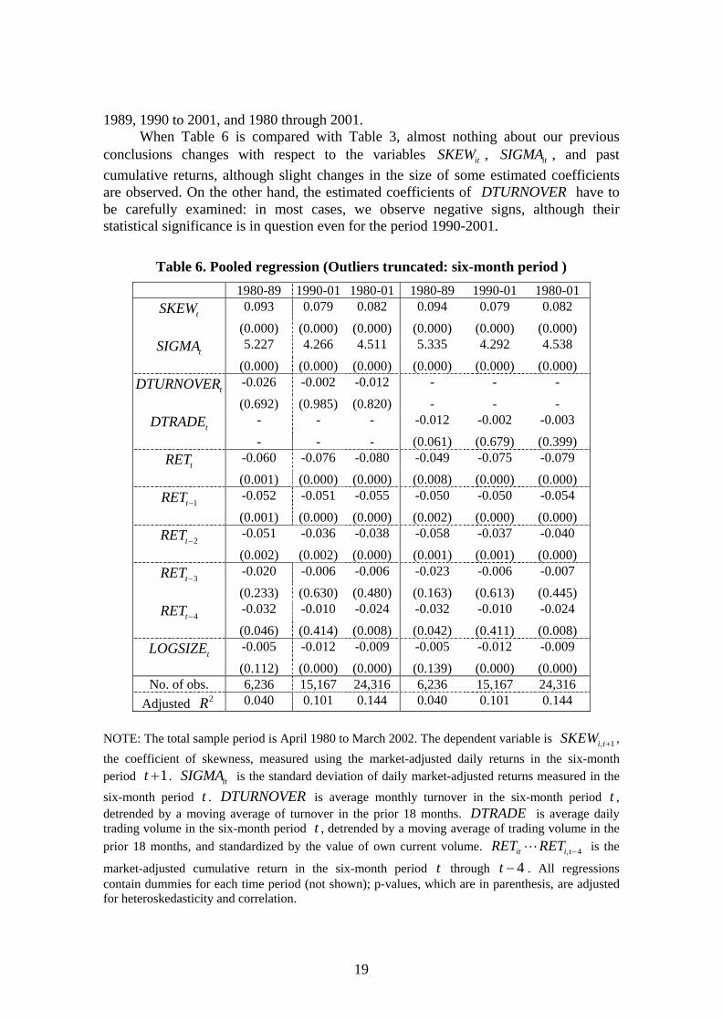
5 Tests for Robustness and a Change in Short-selling Regulations 5.1 Tests with Outliers Truncated To test the robustness of the results presented in the previous section, we conducted further examinations. Because the skewness may be closely related to the values of some outlying samples, robustness tests are conducted by truncating these outliers. Following the method employed in CHS (2001), return data exceeding the value of three times the sample in each period were omitted in constructing a new series of as the ’outliers truncated dataset’. The regression results using this series of are in Table 6 with two alternative trading variables, for 1980 to

itSIGMA t

itSKEW

itSKEW

18

1989, 1990 to 2001, and 1980 through 2001. When Table 6 is compared with Table 3, almost nothing about our previous conclusions changes with respect to the variables , , and past cumulative returns, although slight changes in the size of some estimated coefficients are observed. On the other hand, the estimated coefficients of

itSKEW itSIGMA

DTURNOVER have to be carefully examined: in most cases, we observe negative signs, although their statistical significance is in question even for the period 1990-2001.

Table 6. Pooled regression (Outliers truncated: six-month period ) 1980-89 1990-01 1980-01 1980-89 1990-01 1980-01

tSKEW 0.093 0.079 0.082 0.094 0.079 0.082 (0.000) (0.000) (0.000) (0.000) (0.000) (0.000)

tSIGMA 5.227 4.266 4.511 5.335 4.292 4.538 (0.000) (0.000) (0.000) (0.000) (0.000) (0.000)

tDTURNOVER -0.026 -0.002 -0.012 - - - (0.692) (0.985) (0.820) - - -

tDTRADE - - - -0.012 -0.002 -0.003 - - - (0.061) (0.679) (0.399)

tRET -0.060 -0.076 -0.080 -0.049 -0.075 -0.079 (0.001) (0.000) (0.000) (0.008) (0.000) (0.000)

1tRET − -0.052 -0.051 -0.055 -0.050 -0.050 -0.054 (0.001) (0.000) (0.000) (0.002) (0.000) (0.000)

2tRET − -0.051 -0.036 -0.038 -0.058 -0.037 -0.040 (0.002) (0.002) (0.000) (0.001) (0.001) (0.000)

3tRET − -0.020 -0.006 -0.006 -0.023 -0.006 -0.007 (0.233) (0.630) (0.480) (0.163) (0.613) (0.445)

4tRET − -0.032 -0.010 -0.024 -0.032 -0.010 -0.024 (0.046) (0.414) (0.008) (0.042) (0.411) (0.008)

tLOGSIZE -0.005 -0.012 -0.009 -0.005 -0.012 -0.009 (0.112) (0.000) (0.000) (0.139) (0.000) (0.000)


NOTE: The total sample period is April 1980 to March 2002. The dependent variable is 1i tSKEW , + , the coefficient of skewness, measured using the market-adjusted daily returns in the six-month period . is the standard deviation of daily market-adjusted returns measured in the

six-month period .



tDTRADE

t4it i tRET RET , −L is the

market-adjusted cumulative return in the six-month period t through 4t − . All regressions contain dummies for each time period (not shown); p-values, which are in parenthesis, are adjusted for heteroskedasticity and correlation.

19

In the usual case of testing robustness by truncating outliers, a better fit of the

model is expected. Here, however, we have less explanatory power. Is this bad news? We think it is not, as we are concerned about outliers creating skewness in the return distribution. Thus, it is quite natural when we end up with a worse fitting. We should note the important role of the outlying sample in constructing the theoretical model. 5.2 The Choice of a Time Horizon for Measuring Skewness A six-month horizon is not inherent in the theory. Rather, it is a matter of empirical tests. Thus, we test a three-month period. For this, we focus on data in the 1990s and later because bubble-period data appear to be less appropriate. (The model studied here is not derived to explain bubbles.) Summary statistics are in Table 7.

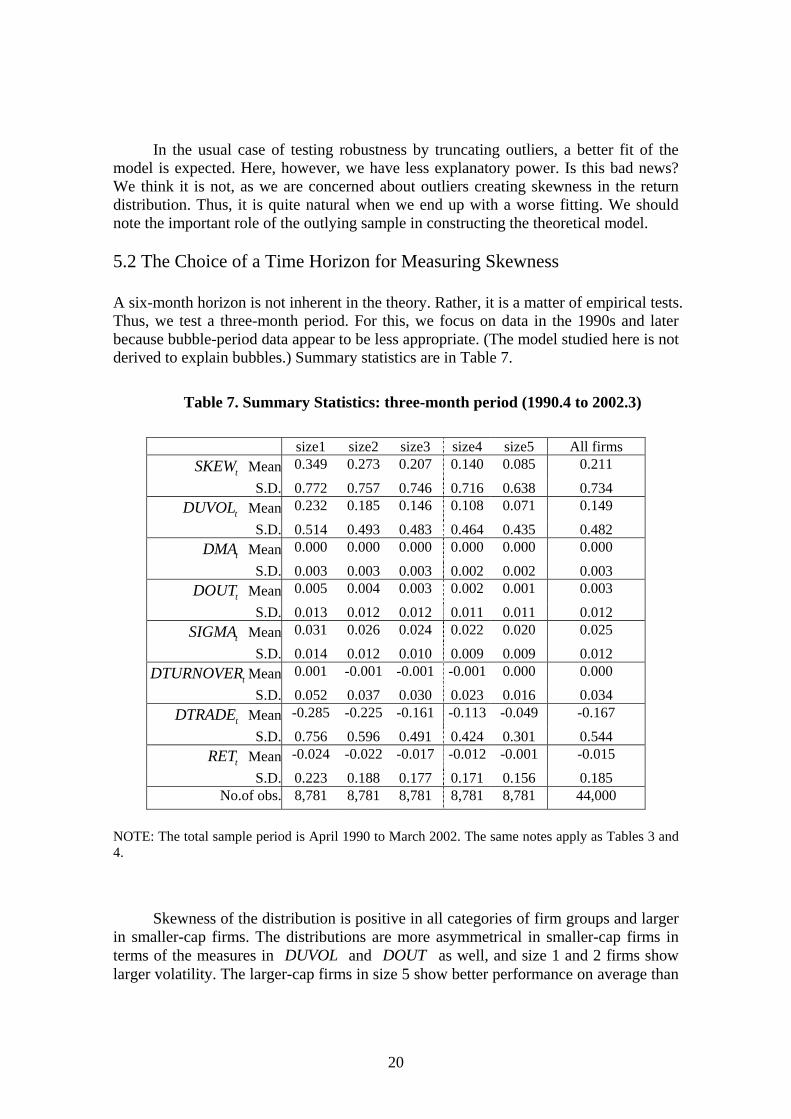
Table 7. Summary Statistics: three-month period (1990.4 to 2002.3)

size1 size2 size3 size4 size5 All firms

tSKEW Mean 0.349 0.273 0.207 0.140 0.085 0.211

S.D. 0.772 0.757 0.746 0.716 0.638 0.734

tDUVOL Mean 0.232 0.185 0.146 0.108 0.071 0.149

S.D. 0.514 0.493 0.483 0.464 0.435 0.482

tDMA Mean 0.000 0.000 0.000 0.000 0.000 0.000

S.D. 0.003 0.003 0.003 0.002 0.002 0.003

tDOUT Mean 0.005 0.004 0.003 0.002 0.001 0.003

S.D. 0.013 0.012 0.012 0.011 0.011 0.012

tSIGMA Mean 0.031 0.026 0.024 0.022 0.020 0.025 S.D. 0.014 0.012 0.010 0.009 0.009 0.012

tDTURNOVER Mean 0.001 -0.001 -0.001 -0.001 0.000 0.000 S.D. 0.052 0.037 0.030 0.023 0.016 0.034

tDTRADE Mean -0.285 -0.225 -0.161 -0.113 -0.049 -0.167 S.D. 0.756 0.596 0.491 0.424 0.301 0.544

tRET Mean -0.024 -0.022 -0.017 -0.012 -0.001 -0.015 S.D. 0.223 0.188 0.177 0.171 0.156 0.185 No.of obs. 8,781 8,781 8,781 8,781 8,781 44,000

NOTE: The total sample period is April 1990 to March 2002. The same notes apply as Tables 3 and 4.

Skewness of the distribution is positive in all categories of firm groups and larger

in smaller-cap firms. The distributions are more asymmetrical in smaller-cap firms in terms of the measures in DUVOL and DOUT as well, and size 1 and 2 firms show larger volatility. The larger-cap firms in size 5 show better performance on average than

20

smaller-cap ones, as seen in the higher value in itRET . These characteristics are basically the same as for the dataset for a six-month periods in Table 2.

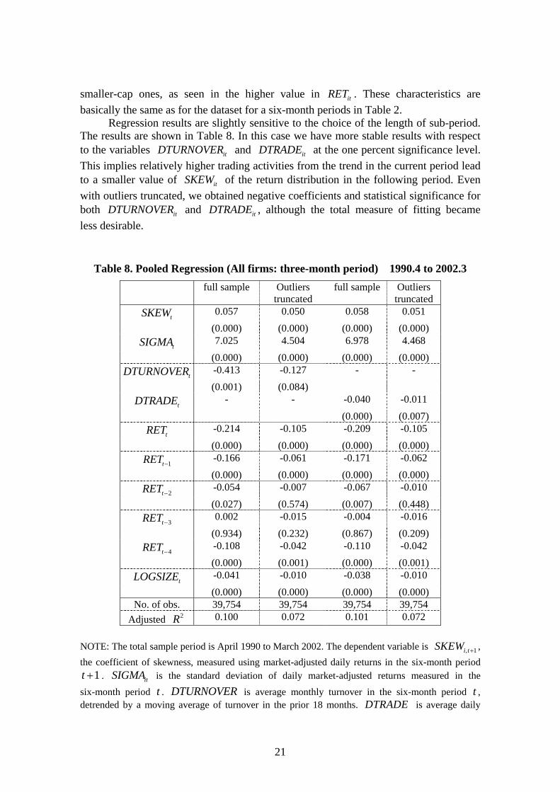
Regression results are slightly sensitive to the choice of the length of sub-period. The results are shown in Table 8. In this case we have more stable results with respect to the variables and at the one percent significance level. This implies relatively higher trading activities from the trend in the current period lead to a smaller value of of the return distribution in the following period. Even with outliers truncated, we obtained negative coefficients and statistical significance for both and , although the total measure of fitting became less desirable.

itDTURNOVER itDTRADE

itSKEW

itDTURNOVER itDTRADE

Table 8. Pooled Regression (All firms: three-month period) 1990.4 to 2002.3 full sample Outliers

truncated full sample Outliers

truncated

tSKEW 0.057 0.050 0.058 0.051 (0.000) (0.000) (0.000) (0.000)

tSIGMA 7.025 4.504 6.978 4.468 (0.000) (0.000) (0.000) (0.000)

tDTURNOVER -0.413 -0.127 - - (0.001) (0.084)

tDTRADE - - -0.040 -0.011 (0.000) (0.007)

tRET -0.214 -0.105 -0.209 -0.105 (0.000) (0.000) (0.000) (0.000)

1tRET − -0.166 -0.061 -0.171 -0.062 (0.000) (0.000) (0.000) (0.000)

2tRET − -0.054 -0.007 -0.067 -0.010 (0.027) (0.574) (0.007) (0.448)

3tRET − 0.002 -0.015 -0.004 -0.016 (0.934) (0.232) (0.867) (0.209)

4tRET − -0.108 -0.042 -0.110 -0.042 (0.000) (0.001) (0.000) (0.001)

tLOGSIZE -0.041 -0.010 -0.038 -0.010 (0.000) (0.000) (0.000) (0.000)

No. of obs. 39,754 39,754 39,754 39,754 Adjusted 2R 0.100 0.072 0.101 0.072



six-month period .


detrended by a moving average of turnover in the prior 18 months. is average daily t

DTRADE

21

trading volume in the six-month period , detrended by a moving average of trading volume in the prior 18 months, and standardized by the value of own current volume.

t4it i tRET RET , −L is the

market-adjusted cumulative return in the six-month period t through 4t − . All regressions contain dummies for each time period (not shown); p-values, which are in parenthesis, are adjusted for heteroskedasticity and correlation.

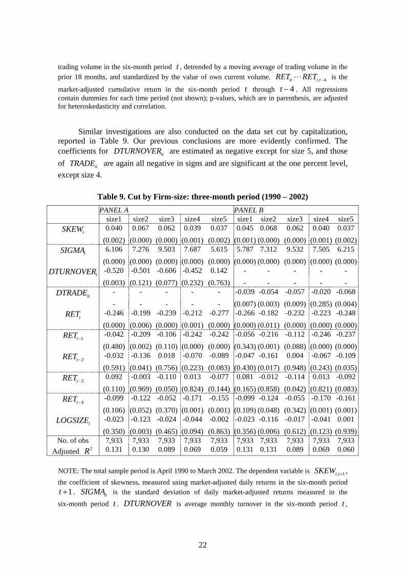
Similar investigations are also conducted on the data set cut by capitalization, reported in Table 9. Our previous conclusions are more evidently confirmed. The coefficients for are estimated as negative except for size 5, and those of are again all negative in signs and are significant at the one percent level, except size 4.

itDTURNOVER

itTRADE

Table 9. Cut by Firm-size: three-month period (1990 – 2002) PANEL A PANEL B

size1 size2 size3 size4 size5 size1 size2 size3 size4 size5

tSKEW 0.040 0.067 0.062 0.039 0.037 0.045 0.068 0.062 0.040 0.037 (0.002) (0.000) (0.000) (0.001) (0.002) (0.001) (0.000) (0.000) (0.001) (0.002)

tSIGMA 6.106 7.276 9.503 7.687 5.615 5.787 7.312 9.532 7.505 6.215 (0.000) (0.000) (0.000) (0.000) (0.000) (0.000) (0.000) (0.000) (0.000) (0.000)

tDTURNOVER -0.520 -0.501 -0.606 -0.452 0.142 - - - - - (0.003) (0.121) (0.077) (0.232) (0.763) - - - - -

itDTRADE - - - - - -0.039 -0.054 -0.057 -0.020 -0.068 - - - - - (0.007) (0.003) (0.009) (0.285) (0.004)

tRET -0.246 -0.199 -0.239 -0.212 -0.277 -0.266 -0.182 -0.232 -0.223 -0.248 (0.000) (0.006) (0.000) (0.001) (0.000) (0.000) (0.011) (0.000) (0.000) (0.000)

1tRET − -0.042 -0.209 -0.106 -0.242 -0.242 -0.056 -0.216 -0.112 -0.246 -0.237 (0.480) (0.002) (0.110) (0.000) (0.000) (0.343) (0.001) (0.088) (0.000) (0.000)

2tRET − -0.032 -0.136 0.018 -0.070 -0.089 -0.047 -0.161 0.004 -0.067 -0.109 (0.591) (0.041) (0.756) (0.223) (0.083) (0.430) (0.017) (0.948) (0.243) (0.035)

3tRET − 0.092 -0.003 -0.110 0.013 -0.077 0.081 -0.012 -0.114 0.013 -0.092 (0.110) (0.969) (0.050) (0.824) (0.144) (0.165) (0.858) (0.042) (0.821) (0.083)

4tRET − -0.099 -0.122 -0.052 -0.171 -0.155 -0.099 -0.124 -0.055 -0.170 -0.161 (0.106) (0.052) (0.370) (0.001) (0.001) (0.109) (0.048) (0.342) (0.001) (0.001)

tLOGSIZE -0.023 -0.123 -0.024 -0.044 -0.002 -0.023 -0.116 -0.017 -0.041 0.001 (0.350) (0.003) (0.465) (0.094) (0.863) (0.356) (0.006) (0.612) (0.123) (0.939)

No. of obs 7,933 7,933 7,933 7,933 7,933 7,933 7,933 7,933 7,933 7,933 Adjusted 2R 0.131 0.130 0.089 0.069 0.059 0.131 0.131 0.089 0.069 0.060



six-month period .

1t + itSIGMAt DTURNOVER is average monthly turnover in the six-month period , t

22


DTRADEt

4it i tRET RET , −L is the

market-adjusted cumulative return in the six-month period through t 4t − . Capitalization groups are quintiles, with group 5 the largest. All regression contains dummies for each time period (not shown); p-values, which are in parenthesis, are adjusted for heteroskedasticity and correlation.

In summarizing the six-month and three-month results, the variables of current , , and SKEW SIGMA RET are shown to be statistically significantly related to the

skewness in the following period. In general, the model we tested has shown better performance with data measured over a three-month period and for the period from 1990 to 2001. For smaller-cap firms categorized in size 1 and 2, the trading pattern in the current period also matters systematically in forecasting the skewness in the next period. These observations are robust in the choice of the length of groupings of data and the choice of the proxy variable to represent difference of opinions as either DTURNOVER or in our research. DTRADE 5.3 Effects of Regulatory Change We have a good opportunity to test the effects of a change in regulations on short-selling. In February 2002, new guidelines were enacted requiring a short sale to be on an up-tick when markets were in down trend. That is, the short-sale had to be at a price higher than the previous trade. Prior regulations allowed shorting at the same price as the previous trade.11 The background of this change was alleged misconduct by several brokerage firms in the preceding several months. At the same time, at the request of the Financial Service Agency (FSA), the share-lending system was reviewed by firms engaged in lending. The FSA asked that changes be made so that borrowers bore the relevant costs. For example, Japan Securities Finance Co., Ltd, introduced new fees for stock-lending, starting from May 7, 2002. The direction of this change is obvious, so we tested its effects. The data between June 2000 and November 2003 are sorted according to the period before and after the change.12 To check whether skewness and associated relationships of the variables differ between these two sub periods, first statistics are calculated, then regressions are conducted.

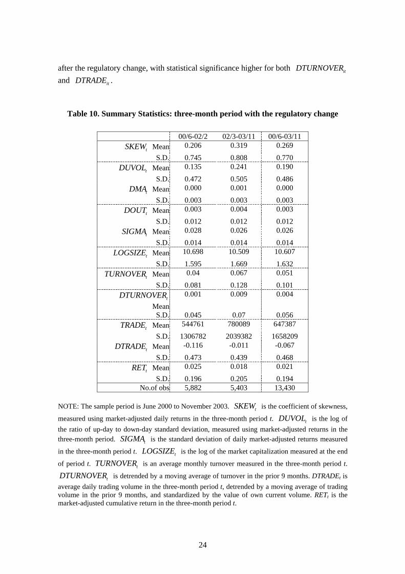
In Table 10, measures indicating asymmetry all have higher values after the regulatory change, but these are not decisive if we consider the size of the standard deviation. Interesting results are obtained in the three regression analyses summarized in Table 11.

As in previous examinations, general observations on variables , , itSKEW itSIGMARET and , hold in a similar way. The results regarding the role of trading variables are very impressive; it appears that the proposed model fits better in the period

itLOGSIZE

11The United States has long had such an "up-tick" rule. This new rule was effective since March 6, 2002. 12Note that the whole sample period here corresponds to the data after the full deregulation of brokerage fees.

23

after the regulatory change, with statistical significance higher for both and .

itDTURNOVER

itDTRADE

Table 10. Summary Statistics: three-month period with the regulatory change

00/6-02/2 02/3-03/11 00/6-03/11

tSKEW Mean 0.206 0.319 0.269

S.D. 0.745 0.808 0.770

tDUVOL Mean 0.135 0.241 0.190

S.D. 0.472 0.505 0.486

tDMA Mean 0.000 0.001 0.000

S.D. 0.003 0.003 0.003

tDOUT Mean 0.003 0.004 0.003 S.D. 0.012 0.012 0.012

tSIGMA Mean 0.028 0.026 0.026 S.D. 0.014 0.014 0.014

tLOGSIZE Mean 10.698 10.509 10.607 S.D. 1.595 1.669 1.632

tTURNOVER Mean 0.04 0.067 0.051 S.D. 0.081 0.128 0.101

tDTURNOVERMean

0.001 0.009 0.004

S.D. 0.045 0.07 0.056

tTRADE Mean 544761 780089 647387 S.D. 1306782 2039382 1658209

tDTRADE Mean -0.116 -0.011 -0.067 S.D. 0.473 0.439 0.468

tRET Mean 0.025 0.018 0.021 S.D. 0.196 0.205 0.194 No.of obs 5,882 5,403 13,430

NOTE: The sample period is June 2000 to November 2003. is the coefficient of skewness,

measured using market-adjusted daily returns in the three-month period t. is the log of the ratio of up-day to down-day standard deviation, measured using market-adjusted returns in the three-month period. is the standard deviation of daily market-adjusted returns measured

in the three-month period t. is the log of the market capitalization measured at the end

of period t. is an average monthly turnover measured in the three-month period t.

is detrended by a moving average of turnover in the prior 9 months. DTRADE

tSKEW

tDUVOL

tSIGMA

tLOGSIZE

tTURNOVER

tDTURNOVER t is average daily trading volume in the three-month period t, detrended by a moving average of trading volume in the prior 9 months, and standardized by the value of own current volume. RETt is the market-adjusted cumulative return in the three-month period t.

24

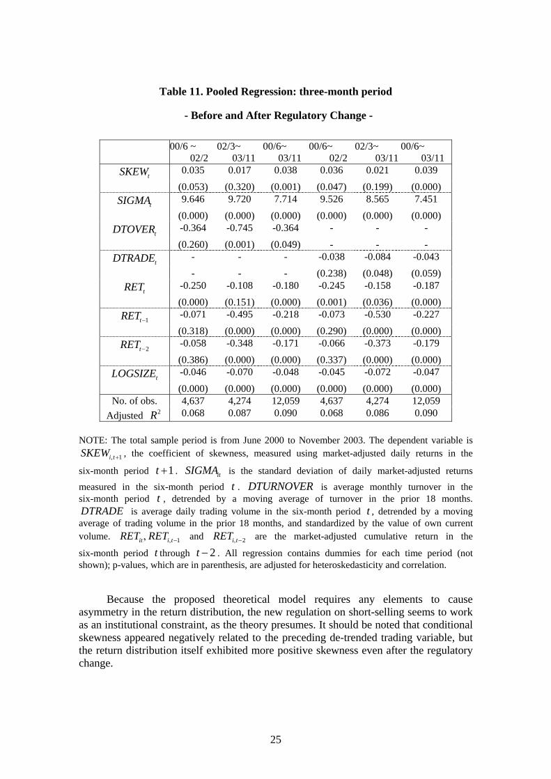
Table 11. Pooled Regression: three-month period

- Before and After Regulatory Change -

00/6 ~ 02/2

02/3~ 03/11

00/6~ 03/11

00/6~ 02/2

02/3~ 03/11

00/6~ 03/11

tSKEW 0.035 0.017 0.038 0.036 0.021 0.039 (0.053) (0.320) (0.001) (0.047) (0.199) (0.000)

tSIGMA 9.646 9.720 7.714 9.526 8.565 7.451 (0.000) (0.000) (0.000) (0.000) (0.000) (0.000)

tDTOVER -0.364 -0.745 -0.364 - - - (0.260) (0.001) (0.049) - - -

tDTRADE - - - -0.038 -0.084 -0.043 - - - (0.238) (0.048) (0.059)

tRET -0.250 -0.108 -0.180 -0.245 -0.158 -0.187 (0.000) (0.151) (0.000) (0.001) (0.036) (0.000)

1tRET − -0.071 -0.495 -0.218 -0.073 -0.530 -0.227 (0.318) (0.000) (0.000) (0.290) (0.000) (0.000)

2tRET − -0.058 -0.348 -0.171 -0.066 -0.373 -0.179 (0.386) (0.000) (0.000) (0.337) (0.000) (0.000)

tLOGSIZE -0.046 -0.070 -0.048 -0.045 -0.072 -0.047 (0.000) (0.000) (0.000) (0.000) (0.000) (0.000)


NOTE: The total sample period is from June 2000 to November 2003. The dependent variable is

, the coefficient of skewness, measured using market-adjusted daily returns in the

six-month period . is the standard deviation of daily market-adjusted returns

measured in the six-month period t .

1i tSKEW , +

1t + itSIGMADTURNOVER is average monthly turnover in the

six-month period , detrended by a moving average of turnover in the prior 18 months. is average daily trading volume in the six-month period , detrended by a moving

average of trading volume in the prior 18 months, and standardized by the value of own current volume.

tDTRADE t

1it i tRET RET , −, and 2i tRET , − are the market-adjusted cumulative return in the

six-month period t through . All regression contains dummies for each time period (not shown); p-values, which are in parenthesis, are adjusted for heteroskedasticity and correlation.

2t −

Because the proposed theoretical model requires any elements to cause asymmetry in the return distribution, the new regulation on short-selling seems to work as an institutional constraint, as the theory presumes. It should be noted that conditional skewness appeared negatively related to the preceding de-trended trading variable, but the return distribution itself exhibited more positive skewness even after the regulatory change.

25

6 Concluding Remarks and Future Agenda Although it is well known that the market rate of return tends to show negative skewness, the return distribution of individual stocks has shown positive skewness for several sub groupings. This observation is consistent with the results reported on US capital markets as found in Duffee (1995), CHS (2001) and others. Our analysis here contributes to demonstrating important similarities in the firm-level distribution of returns in the principal Japanese markets. Positive skewness in the returns is more evident for smaller firms. Although CHS (2001) suggest that managers of smaller firms have greater flexibility regarding disclosure, more detailed analysis on why such positive skewness arises is needed. From the analysis of pooled cross-section data of individual stocks, we find clear evidence of predictive power in the information preceding time for the skewness in period . Specifically, the greater the volatility and skewness in the current period, the greater the value of the skewness in the following period. Also, the up trends in own returns in the preceding periods may explain a rather negatively skewed return distribution in the following period. These results are significantly shown for the whole sample period from 1980 to 2001, as well as for two sub periods.

t1t +

The Hong and Stein model predicts a relation between turnover and skewness. As to the explanatory power of preceding trading activity, our analysis shows inconclusive results for the return distribution of individual stocks listed on the first and second sections of the Tokyo Stock Exchange. Such asymmetry can be partly accounted for by the divergence of trading volume from trend. However, the effects of the variable DTURNOVER and TR seem to be not so robust as such other variables as own skewness, volatility, and cumulative rate of return in the preceding period. Still, systematic relations to the skewness measured over both a three-month and a six-month period were more evident in trading variables for small firms in the 1990s through 2001. In this regard, we note the difference in share ownership structure between large and small firms, yet exact logic is not well identified.

ADE

The regulatory change in short-selling that took place in February 2002 appears to have enhanced this negative relation between the size of the value of skewness in the following period and current trading proxies. This suggests that institutional framework is regarded as an important factor to be related to the pattern of return distribution of individual stocks. Overall, our empirical analysis suggests that there is strong evidence that lagged volatility, skewness and returns predict skewness in the current period. Conditional skewness appears partly explained by previous detrended trading proxies, however, the results are not conclusive and the mechanism that creates positive skewness in individual stock returns was not well identified. Our application of the Hong and Stein model to Japanese data does not contracted it, but this is not the same as a definitive support. Further research, both empirical and theoretical, is required.

26

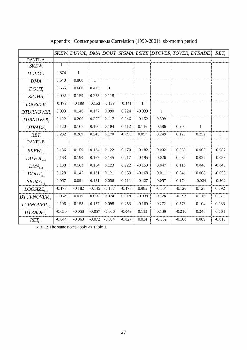
Appendix : Contemporaneous Correlation (1990-2001): six-month period

tSKEW tDUVOL tDMA tDOUT tSIGMA tLSIZE tDTOVER tTOVER tDTRADE tRET

PANEL A

tSKEW 1

tDUVOL 0.874 1

tDMA 0.540 0.800 1

tDOUT 0.665 0.660 0.415 1

tSIGMA 0.092 0.159 0.225 0.118 1

tLOGSIZE -0.178 -0.188 -0.152 -0.163 -0.441 1

tDTURNOVER 0.093 0.146 0.177 0.090 0.224 -0.039 1

tTURNOVER 0.122 0.206 0.257 0.117 0.346 -0.152 0.599 1

tDTRADE 0.120 0.167 0.166 0.104 0.112 0.116 0.586 0.204 1

tRET 0.232 0.269 0.243 0.170 -0.099 0.057 0.249 0.128 0.252 1

PANEL B

1tSKEW + 0.136 0.150 0.124 0.122 0.170 -0.182 0.002 0.039 0.003 -0.057

1tDUVOL + 0.163 0.190 0.167 0.145 0.217 -0.195 0.026 0.084 0.027 -0.058

1tDMA + 0.138 0.163 0.154 0.123 0.222 -0.159 0.047 0.116 0.048 -0.049

1tDOUT + 0.128 0.145 0.121 0.121 0.153 -0.168 0.011 0.041 0.008 -0.053

1tSIGMA + 0.067 0.091 0.131 0.056 0.611 -0.427 0.057 0.174 -0.024 -0.202

1tLOGSIZE + -0.177 -0.182 -0.145 -0.167 -0.473 0.985 -0.004 -0.126 0.128 0.092

1tDTURNOVER + 0.032 0.019 0.000 0.024 0.018 -0.038 0.128 -0.193 0.116 0.071

1tTURNOVER + 0.106 0.158 0.177 0.098 0.253 -0.169 0.272 0.578 0.104 0.083

1tDTRADE + -0.030 -0.058 -0.057 -0.036 -0.049 0.113 0.136 -0.216 0.248 0.064

1tRET + -0.044 -0.060 -0.072 -0.034 -0.027 0.034 -0.032 -0.108 0.009 -0.010

NOTE: The same notes apply as Table 1.

27

References [1] Barberis, N. and R. Thaler, 2003, “A Survey of Behavioral Finnace”, in Constantinides, G. M., M. Harris, and R. M. Stulz eds, Handbook of the Economics of Finance: Financial Markets and Asset Pricing (Handbooks in Economics, Bk. 21), Elsevier, North-Holland. [2] Bekaert, G., and G. Wu, 2000, “Asymmetric volatility and risk in equity markets”, Review of Financial Studies, 13, 1-42. [3] Chen, J., H. Hong, and J. C. Stein, 2001, “Forecasting Crashes: Trading Volume, Past Returns and Conditional Skewness in Stock Prices”, Journal of Financial Economics, 61, 345-381. [4] Cristie, A. A., 1982, “The stochastic behavior of common stock variances - value, leverage and interest rate effects”, Journal of Financial Economics, 10, 407-432. [5] Duffee, G. R., 1995, “Stock Returns and Volatility A Firm-level Analysis”, Journal of Financial Economics, 37, 399-420. [6] Engle, R., and V. K. Ng, 1993, “Measuring and Testing the impact of News on Volatility”, Journal of Finance, 48, 1749-1778. [7] Glosten, L., R. Jaganathan and D. Runkle, 1993, “On the Relationship between the Expected Value and the Volatility of the Nominal Excess Return on stocks”, Journal of Finance, 48, 1779-1801. [8] Harris, M., and A. Raviv, 1993, “Differences of Opinion Make a Horse Race”, Review of Financial Studies, 6, 473-506. [9] Harvey, C. R., and A. Siddique, 2000, “Conditional skewness in asset pricing tests”, Journal of Finance, 55, 1263-1295. [10] Hong, H., and J. C. Stein, 2003, “Differences of Opinion, Short-Sales Constraints, and Market Crashes”, Review of Financial Studies, 16, 487-525. [11] Kandel, E, and N. D. Pearson, 1995, “Differential interpretation of public signals and trade in speculative markets”, Journal of Political Economy, 103, 831-872. [12] Odean, T., 1998, “Volume, volatility, price and profit when all traders are above average”, Journal of Finance, 53, 1887-1934. [13] Schwert, G. W. 1989. “Why does stock market volatility change over time?”, Journal of Finance, 44, 1115-1153.

28

Forecasting skewness in stock returns: Evidence from firm ...

Documents

Transcript of Forecasting skewness in stock returns: Evidence from firm ...