FORECASTING REALIZED (CO)VARIANCES WITH A BLOC STRUCTURE WISHART AUTOREGRESSIVE MODEL

MATTEO BONATO MASSIMILIANO CAPORIN ANGELO RANALDO WORKING PAPERS ON FINANCE NO. 2012/11 SWISS INSTITUTE OF BANKING AND FINANCE (S/BF – HSG)

NOVEMBER 2012

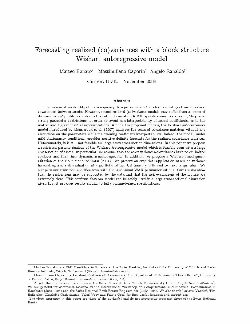
Forecasting realized (co)variances with a block structureWishart autoregressive model

Matteo Bonato� Massimiliano Caporiny Angelo Ranaldoz

Current Draft: November 2008

AbstractThe increased availability of high-frequency data provides new tools for forecasting of variances and

covariances between assets. However, recent realized (co)variance models may su�er from a `curse ofdimensionality' problem similar to that of multivariate GARCH speci�cations. As a result, they needstrong parameter restrictions, in order to avoid non-interpretability of model coe�cients, as in thematrix and log exponential representations. Among the proposed models, the Wishart autoregressivemodel introduced by Gourieroux et al. (2007) analyzes the realized covariance matrices without anyrestriction on the parameters while maintaining coe�cient interpretability. Indeed, the model, undermild stationarity conditions, provides positive de�nite forecasts for the realized covariance matrices.Unfortunately, it is still not feasible for large asset cross-section dimensions. In this paper we proposea restricted parametrization of the Wishart Autoregressive model which is feasible even with a largecross-section of assets. In particular, we assume that the asset variances-covariances have no or limitedspillover and that their dynamic is sector-speci�c. In addition, we propose a Wishart-based gener-alization of the HAR model of Corsi (2004). We present an empirical application based on varianceforecasting and risk evaluation of a portfolio of two US treasury bills and two exchange rates. Wecompare our restricted speci�cations with the traditional WAR parameterizations. Our results showthat the restrictions may be supported by the data and that the risk evaluations of the models areextremely close. This con�rms that our model can be safely used in a large cross-sectional dimensiongiven that it provides results similar to fully parameterized speci�cations.

�Matteo Bonato is a PhD Candidate in Finance at the Swiss Banking Institute of the University of Zürich and SwissFinance Institute, Zürich, Switzerland (E-mail: bonato@isb.uzh.ch.)yMassimiliano Caporin is Assistant Professor of Economics at the Department of Economics �Marco Fanno", University

of Padua, Padua, Italy (E-mail: massimiliano.caporin@unipd.it).zAngelo Ranaldo is senior economist at the Swiss National Bank, Zürich, Switzerland (E-mail: Angelo.Ranaldo@snb.ch).

We are grateful for comments received at the International Workshop on Computational and Financial Econometrics inNeuchatel (June 2008) and the Swiss National Bank Brown Bag Seminar (July 2008). We also thank Loriano Mancini, TimBollerslev, Charlotte Christiansen, Valeri Voev and Fulvio Corsi for they useful feedback and suggestions.-The views expressed in this paper are those of the author(s) and do not necessarily represent those of the Swiss NationalBank-

1 IntroductionThe increased availability of high-frequency data provides new tools for forecasting variances and co-variances between assets. In particular, after the seminal paper by Andersen and Bollerslev (1998), theliterature on realized volatility has grown enormously; see McAleer and Medeiros (2006) for a review.

While most works has focused on the study of univariate series, recently there has been growing theoret-ical and empirical interest in extending the results for the univariate process to a multivariate framework.In this context, two pioneering contributions have been made by Barndor�-Nielsen and Shephard (2004)and Bandi and Russel (2005). Barndor�-Nielsen and Shephard (2004) did not consider the presence ofmicrostructure noise, whereas of the noise has been considered in Bandi and Russel (2005).

Alternative approaches to the high-frequency covariance estimator have recently been introduced byHayashi and Yoshida (2005, 2006), Sheppard (2006) and Zhang (2006), among others. For example, insteadof using calendar returns, the Hayashi and Yoshida estimator (HY) is based on overlapping tick-by-tickreturns. Sheppard (2006) analyzed the conditions under which the realized covariance is an unbiased andconsistent estimator of the integrated covariance. Zhang (2006) also studied the e�ects of microstructurenoise and non-synchronous trading in the estimation of integrated covariance between assets.

Although the literature on multivariate extensions of the realized variance regarding the de�nition ofnew estimators of the realized covariances resulted in a notable amount of academic works, only a fewpapers provide �nancial applications for these new estimators.

One explanation for the scarcity of empirical contributions in multivariate realized volatility analysisis the di�culty in �nding a dynamic speci�cation of a stochastic volatility matrix which satis�es thesymmetry and positivity properties of each forecasted matrix, does not su�er from the so called `curse ofdimensionality' and possesses a closed-form expression for the forecasts at any horizon.

In an interesting paper, de Pooter et al. (2006) investigate the bene�ts of high-frequency intradaydata when constructing mean-variance e�cient stock portfolios with daily rebalancing from the individualconstituents of the S&P 100 index. The author analyzed the issue of determining the optimal samplingfrequency, as judged by the performances of the estimated portfolios. As in Fleming et al. (2001, 2003),and building on the work of Foster and Nelson (1996) and Andreou and Ghysels (2002), in this paper arolling window volatility estimator is used to forecast the conditional variance matrix Vt;h:bVt;h = exp(��h)bVt�1;h + �h exp(��)Yt�1 (1)

where �h can be estimated by means of maximum likelihood for the model

rt = bV 1=2t;h zt (2)

with zt i:i:d:� N(0; I) and Yt as the realized covariance matrix estimated using I intraday returns of equallength h � 1=I. rt is the usual n � 1 vector of daily returns at time t of the n assets composing theportfolio.

In a related paper, Bandi et al. (2006) evaluate the economic bene�ts of methods that have beensuggested to optimally sample (in a MSE sense) high-frequency returns data for the purpose of realizedvariance and covariance estimation in the presence of market microstructure noise. However, their approachis di�erent from that in de Pooter et al. (2006); their method is designed to select the time-varying optimalsampling frequency for each entry in the covariance matrix based on MSE criteria. Subsequently, theeconomic gains yielded by the MSE-based optimal sampling are evaluated by comparing the utility gains

1

provided by optimally sampled realized covariance with realized covariances based on �xed intervals. Toforecast each entry of the covariance matrix, they adopted an ARFIMA(2; d; 2) model.

An alternative way to forecast the realized variance/covariance matrix is to adopt a matrix transfor-mation that guarantees the positive de�nitiveness of the forecasts.

Bauer and Vorkink (2007) present a new matrix logarithm model of realized covariance stock returnswhich uses latent factors as functions of both lagged volatility and returns. The model has several ad-vantages in that it is parsimonious, does not impose parametric restrictions, and yields positive de�nitecovariance matrices.

In Chiriac and Voev (2008) a model based on a multivariate, fractionally integrated autoregressivemoving average (ARMA) process for the elements of the Cholesky factors of the observed matrix seriesis proposed. Denoting with Yt the n � n realized covariance matrix at time t, with n the number ofassets considered, the Cholesky decomposition of Yt is given by the upper triangular matrix Pt, for whichPtP 0t = Yt. Then the following model is used

�(L)D(L)(Xt � �) = �(L)�t; �t � N(0;�t): (3)

Xt = vech(Pt) is the vector obtained by stacking the upper triangular components of the matrix Pt ina vector, �(L) and �(L) are matrix lag polynomials and D(L) = diag[(1 � L)d1 ; : : : ; (1 � L)dm ], whered1; : : : ; dm are the degrees of fractional integration of each of the m elements of the vector Xt. � is a vectorof constants. Parameters in (3) are not directly interpretable. However, the dynamic linkages among thevariances and covariances series as functions of those parameters are derived.

While both the matrix logarithmic transformation and the Cholesky decomposition have the advantageof guaranteeing the positive de�niteness of the covariance matrix, they also have a major drawback: thecoe�cients of the model totally rule out any possible interpretation. In other words, there is no way tocheck the signi�cance of the interactions between variances and covariances and thus to reduce the numberof parameters in the model by imposing no or limited spillover between the variances and covariances.

A solution to this problem is represented by the Wishart autoregressive model (WAR) proposed byGourieroux et al. (2007). The model is based on a dynamic extension of the Wishart distribution. Thisspeci�cation is compatible with �nancial theory, satis�es the constraints on volatility matrices, has a�exible form and, most importantly, maintains the coe�cients' interpretability.

The main innovation proposed in this paper is the introduction of a speci�c parametrization of theWAR model. In particular, we show how to achieve a great reduction of the number of parametersaccording to an economic criterion which is consistent with standard sectorial asset allocation approaches.The parametric structure we propose imposes a block structure on the coe�cient matrices, hence we namethe model block WAR. The use of block structures in parameter matrices is similar to that in Billio et al.(2006), Billio and Caporin (2008), Asai et al. (2008). Engle and Kelly (2008) introduce a block structurefor the correlation matrix while Caporin and Paruolo (2008) present a spatial solutions to the course ofdimensionality problem in multivariate volatility models that implies a block structure on the coe�cientmatrices. In this paper we assume that the asset variances-covariances have no or limited spillover and thattheir dynamic is sector-speci�c. A pairwise preliminary analysis con�rms this assumption and allows us tosubstantially reduce the number of parameters implied by the model. In addition, we propose a Wishart-based generalization of the HAR model of Corsi (2004), named HAR-WAR model. We present an empiricalapplication based on variance forecasting and risk evaluation of a portfolio of two US treasury bills andtwo exchange rates. We compare our restricted speci�cations with the traditional WAR parameterizations.

2

Our results show that the restrictions may be supported by the data and that the risk evaluations of themodels are extremely close. This con�rms that our model can be safely used in a large cross-sectionaldimension given that it provides results similar to fully parameterized speci�cations.

Section 2 introduces the WAR model of Gourieroux et al. (2007), followed by our proposed generaliza-tion. Section 3 presents the estimation procedure and show an alternative way to estimate the degrees offreedom of the model, a key element to determine if the density of the Wishart distribution exists. Thedataset we used is presented in Section 4 and an empirical application based on portfolio risk evaluationis provided in Section 5. Section 6 concludes and gives directions for future research.

2 The block Wishart autoregressive modelIn the following we de�ne the basic Wishart auto regressive model of Gourieroux et al. (2007) and thenwe introduce the set alternative parametric restrictions that de�ne the block WAR.

2.1 The Wishart Autoregressive ModelDenote by Yt the time t (realized) covariance for a group of n assets. The sequence of stochastic positivede�nite Yt matrices is said to follow a Wishart process if the following relations hold.

At �rst, the (realized) covariance may be represented as a sum of underlying stochastic processes

Yt =KXk=1

xk;tx0k;t; (4)

where xk;t; k = 1; 2; : : : ;K are independent Gaussian VAR(1) processes of dimension n with a commonautoregressive parameter matrix M and common innovation variance �:

xk;t = Mxk;t�1 + �k;t; �k;t � N(0;�): (5)

When Yt is de�ned as in (4) and (5) we say it follows a WAR process of order 1, denoted W [K;M;�]. Thetransition density of WAR(1) depends on the following parameters: K, the scalar degree of freedom (thenumber of underlying VAR processes), strictly greater that n-1 (the number of assets minus one); M , then � n matrix of autoregressive parameters; and �, the n � n symmetric and positive de�nite matrix ofinnovation covariances. We stress that the interpretation of Yt from latent Gaussian VAR(1) processes isvalid for integer valued K only.

From Proposition 2 in Gourieroux et al. (2007) we have:

Et (Yt+1) = MYtM 0 +K�: (6)

The �rst conditional moment is thus an a�ne function of the lagged values of the volatility process.In particular, the WAR(1) process is a weak linear AR(1) process. More precisely we get:

Yt+1 = MYtM 0 +K� + �t+1; (7)

where �t+1 is a matrix of stochastic errors with a zero conditional mean. Equivalently, we may representYt conditional mean in the following companion form:

vech(Yt+1) = A(M)vech(Yt) + vech(K�) + vech(�t+1); (8)

3

where vech(Y ) denotes the vector obtained by stacking the lower triangular elements of Y , and A(M)is a function of M . The error term � is a weak white noise, since it features conditional heteroskedasticityand, even after conditional standardization, is not identically distributed.

In general, WAR processes with higher autoregressive order p may be considered and the Wishartprocess can be easily extended to include more autoregressive lags. This is accomplished by replacing theconditioning matrix MYtM 0 with any symmetric positive semi-de�nite function of Yt; Yt�1; : : : ; Yt�p+1.However, when the autoregressive order is larger than 1, the interpretation of the Wishart process as thesum of squares of autoregressive Gaussian processes in no longer valid even for integer K. For a WAR(p)process, the equivalent of (6) reads:

Et (Yt+1) =pXj=1

MjYt+1�jM 0j +K�: (9)

In the following, unless di�erently stated, we will refer only to WAR(1) speci�cations.

2.2 Interpretation of the coe�cientsThe principal drawback of many multivariate volatility models is the so-called `curse of dimensionality',that is, the numbers of parameters is a power function of the cross-sectional model dimension. One of themain contributions of this paper is to provide a sensible reduction of the parameter space by imposing aset of restrictions on the standard WAR model. Our modeling approach will be presented in the followingsection; here we provide the intuition on parameter interpretation within the WAR model.

In the simple case of a (2� 2) matrix, as done in Gourieroux (2007), we de�ne the best prediction ofYt given by a WAR(1) model. Then we present the approaches we suggest to reduce the parameter space.

Consider the (2� 2) covariance matrix Yt, the autoregressive matrix M and the innovation variance �:

Yt =

Y11;t Y12;t

Y12;t Y22;t

!;M =

m11 m12

m21 m22

!and � =

�11 �12

�12 �22

!The full WAR(1) model speci�es the best prediction of Yt as:

E[YtjYt�1] =

a1Y11;t�1 + b1Y12;t�1 + c1Y22;t�1 + d1 a2Y11;t�1 + b2Y12;t�1 + c2Y22;t�1 + d2

� a3Y11;t�1 + b3Y12;t�1 + c3Y22;t�1 + d3

!(10)

where aj ; bj ; cj and dj ; j = 1; : : : ; 3 are scalar parameters. dj corresponds to K times the entries of �.By construction, the prediction is a symmetric semi-de�nite positive matrix for any Yt�1 which belong toS+, the set of symmetric positive de�nite matrices. To express it in terms of M we have:8>><>>:

a1 = m211; b1 = 2m11m12; c1 = m2

12;a2 = m11m21; b2 = m11m22 +m21m21; c2 = m12m22;a3 = m2

21; b3 = 2m21m22; c3 = m222;

The e�ect of the past variances and covariances on the present volatility can be seen immediately.First, note that the full WAR model allows for spillover between variances and covariances.

Therefore, a possible strategy is to reduce the numbers of parameters by assuming no or limitedspillover between the variances. For instance, setting m12 = 0 implies that the conditional variance ofthe �rst asset depends only on its past shocks and that the second asset variance does not in�uence the

4

conditional covariance. Di�erently, a diagonal speci�cation of M corresponds to the absence of spilloversbetween variances and covariances.

This very simple example in two dimensions helps us to identify the coe�cients in M that plays arole in the spillover e�ect between variances. Using the delta method we can, in fact, easily computethe standard errors for the ai; bi and ci and thus evaluate which parameters are signi�cant and check theappropriateness of assumption of limited spillover. We will present now four di�erent parametrizationsfor the WAR process that impose no or limited spillover. We also show in the empirical analysis that therestrictions we impose on the matrix M are justi�ed by the data.

2.3 Speci�cations of the block Wishart autoregressive modelTo derive the block WAR model we impose a set of restrictions on the matrix M . These restrictions comefrom a criterion allowing assets to be grouped. Some examples are given by the economic sector of thestocks entering into an equity portfolio, the type of assets entering into a diversi�ed equity-bond portfolio,or the geographical reference areas of a group of assets. The main intuition behind asset grouping is thatthe clustered variables may share common patterns or common features, and that their variance-covariancedynamic is similar. In fact, we can presume that assets belonging to the same economic sector may havea similar reaction to market shocks/news, and are similarly a�ected by market movements.

Clearly, groups may be de�ned on a data-driven basis, such as referring to the dynamic propertiesof the series mean and/or variances, or on mixed criteria. The comparison of alternative methods forclustering �nancial assets is outside the scope of this paper and will not be considered. In the following wewill use a priori de�ned groups in order to present our modeling approach and to show, on an empiricalbasis, its advantages.

Consider the simple WAR(1) model as in Eq. 7:

Yt+1 = MYtM 0 +K� + �t+1:

Assume that our portfolio consists of n stocks and that we can classify them into N groups, accordingto some economic (or data-driven) criterion, as discussed in the previous section (such as the economicsector or the existence of common patterns in realized variances and covariances).

The N groups have dimension ni withPi ni = n. In addition, the assets are ordered following a group

rule, that is, assets from 1 to n1 belong to group 1, assets from n1 + 1 to n1 + n2 belongs to group 2, andso on. Given this asset classi�cation, the autoregressive matrix M may be partitioned as follows:

M =

0BB@ M11 � � � M1N... Mii

...MN1 � � � MNN

1CCA ;

where Mij is a matrix of dimension ni � nj .By imposing a particular structure on the matricesMij we be able to reduce the number of parameters

of the model. We propose the following speci�cations:

(i) Mij = 0 8i 6= j; i; j = 1; : : : ; N ,

(ii) Mij = 0 and Mii = �i(ini i0ni); 8i 6= j; i; j = 1; : : : ; N

(iiii) Mij = 0 and Mii = (�i;1; : : : ; �i;ni)(Ini); 8i 6= j; i; j = 1; : : : ; N

5

(iv) Mij = 0 and Mii = �i(Ini); 8i 6= j; i; j = 1; : : : ; N

where ini is a ni � 1 vector of ones and Ini is the identity matrix of dimension ni.If assets belonging to the same group share common reactions to shocks, we can hypothesize, to some

extent, that their co-volatilities also have a similar behavior. If the groups are sector-speci�c, model (i)implies that the variances and covariances of each asset are only in�uenced by the variances and covariancesof assets belonging to the same class. Therefore, no volatility spillover exists between assets belonging todi�erent sectors. We named this model block WAR. The number of parameters that needs to be estimatedis n(n+ 1)=2 +

PNi=1 n

2i , along with the degrees of freedom K.

A further reduction of the number of parameters is obtained by imposing a single parameter for eachgroup, as shown in model (ii). In this case, the variance and covariance of each asset belonging to, say,group j depends on the past values of itself, on the past values of the variances of the other assets of thesame group and on the covariances with those assets via a function of the unique parameter �j . We callthis model restricted block WAR. This models contains n(n+ 1)=2 +N parameters in M and � plus K.

Model (iii) relaxes the assumption of spillover between assets belonging to the same sector. It assumeseach matricx Mii; i = 1; : : : ; Ni to be diagonal, i.e. the autoregressive matrix M is diagonal. In this casegrouping the assets according to some criterion does not a�ect the parametric space. We named this modeldiagonal WAR. For this model, n parameters need to be estimated in the matrix M , plus the n(n+ 1)=2parameters in � and the degrees of freedom K. One of the implications of the diagonal structure for Mis that each realized variance is only a function of its past values.

If we assume again that assets belonging to the same sector have common dynamics for the variance,or if we can �nd a way to group assets whose volatilities obeys the same process, the number of parameterscan be further reduced. This is the case for model (iv). For each group a single parameter is taken to modelthe dynamics of the variances for the assets in the considered group, i.e. the elements on the diagonal ofeach Mii; i = 1; : : : ; N are all equal. In total only N + n(n + 1)=2 + 1 parameters are required in thismodel. We refer to this model as the restricted diagonal WAR.

Is is worth mentioning that the speci�cations (i)-(iv) do not represent a complete generalization of theWAR model. In fact, we set all the o�-diagonal blocks to zero. The assumption Mij = 0 8i 6= j; i; j =1; : : : ; N can be replaced by the same structure we imposed on the matrices Mii: full, scalar, diagonal andrestricted diagonal. This allows us to consider not only the interactions between assets belonging to thesame group, but also interactions between a limited set of groups. In this paper we stick with a structurethat ignores the o�-diagonal blocks and leave a full generalization of the WAR model for future works.

2.4 The block HAR-WAR modelOne of the stylized facts about asset returns is the long-run temporal dependencies of return volatilities.The literature on volatility modeling has documented that such temporal dependencies are highly per-sistent. In particular, the low �rst-order autocorrelations usually found in empirical analysis (Thomakosand Wang, 2003), along with their slow decay, suggest that the logarithmic realized standard deviationsdo not contain a unit root but exhibit long memory.

To account for this, fractionally integrated autoregressive models (ARFIMA) have been shown to bee�ective in empirical modeling (see Andersen et al. (2001a) and Andersen et al. (2001b) among others).Fractional integration achieves long memory parsimoniously by imposing a set of in�nite dimensionalrestrictions on the in�nite variable lags but completely lacks a clear mathematical interpretation.

6

Another crucial point is that the long memory observed in the data could be only an apparent behaviorgenerated from a process which is not really long memory. Indeed, the usual tests can indicate the presenceof long memory simply because the largest aggregation level that we are able to consider is not large enough.LeBaron (2001) shows that a very simple additive model de�ned, as the sum of only three di�erent linearprocesses (AR(1) processes) each operating on a di�erent time frame, can display hyperbolic decayingmemory, provided that the longest component has a half-life that is long relative to the test aggregationranges. Another result from Granger (1980) shows that the sums of an high number of short memoryprocesses can induce long memory. In Pong et al. (2004) an ARMA(2,1) is proposed to model and forecastrealized volatility. The authors' choice is motivated by the research of Gallant et al. (1999), who show thatthe sum of two AR(1) processes is capable of capturing the persistent nature of asset price volatility. Intheir paper Pong et al. (2004) show that the short memory ARMA(2,1) model is as good as long memoryARFIMA models when forecasting futures volatilities. Motivated by the existence of multiple volatilitycomponents in intraday frequencies, along with the apparent long-memory characteristic, Andersen andBollerslev (1997) formulated a version of the mixture-of-distributions hypothesis (MDH) for returns thatexplicitly accommodates numerous heterogeneous information arrival processes.

An alternative to ARFIMA is the heterogeneous autoregressive (HAR) model suggested by Corsi (2004)(see also Aït-Sahalia and Mancini, 2008; Corsi et al., 2007). Extending the heterogeneous ARCH model ofMüller et al. (1997), the long-memory pattern is reproduced by summing of (a small number of) volatilitycomponents constructed over di�erent horizons. The basic ideas stems from the so called `heterogeneousmarket hypothesis' presented by Müller et al. (1993), which recognized the presence of heterogeneity intraders. Di�erently from Andersen and Bollerslev (1997), in this latter view the multi-component structurein the volatility is to be found in the heterogeneity of agents rather than in the heterogeneous nature ofthe information arrival.

De�ning the k-period realized volatility component by the sum of the single-period realized volatilities,i.e. �p

RV�t�k:t�1

=1k

kXj=1

pRVt�j ; (11)

the HAR model for realized volatility of Corsi (2004), including the daily, weekly and monthly realizedvolatility components, is given by

pRV t = �0 + �d +

pRV t�1 + �w

�pRV�t�5:t�1

+ �m�p

RV�t�22:t�1

+ �t: (12)

In Corsi (2004) �t is assumed to be Gaussian white noise., whereas in Corsi et al. (2007), a standardizednormal inverse Gaussian (NIG) is chosen to deal with the non-Gaussianity of the error terms.

In the spirit of the HAR model, we propose here to model the conditional realized covariance matrixYt with an autoregressive Wishart process which accounts for the temporal aggregation of the covariancematrix. We call this process WAR-HAR process. In the sequel, we will show that this process, can beinterpreted as a particular WAR(23) process.

De�ne the k-period realized covariance matrix component by the sum of the single-period realizedcovariance matrices:

Yt�k:t�1 =1k

KXj=1

Yt�j (13)

Combining a WAR(p) structure with the temporal aggregation induced by the HAR model, we write the

7

process Yt as:Yt = M1Yt�1M 01 +M2Yt�5:t�1M 02 +M3Yt�22:t�1M 03 +K� + �t; (14)

Now, opening the summations and aggregating according to the same lag, we get:

Yt = (M1Yt�1M 01) +�

~M2Yt�1 ~M 02 + ~M3Yt�1 ~M 03�

+ � � �+ (15)�~M2Yt�5 ~M 02 + ~M3Yt�5 ~M 03

�+ ~M3Yt�6 ~M 03 + � � �+ ~M3Yt�22 ~M 03 + (16)

K� + �t; (17)

with ~M2 = 1p5M2 and ~M3 = 1p

22M3.

To interpret the process as a WAR(22), we simply rewrite it as:

Yt = M1Yt�1M 01 +5Xi=1

N2Yt�iN 02 +23Xj=6

~M3Yt�j ~M 03 +K� + �t: (18)

where

N2 : N2YtN 02 = ~M2Yt ~M 02 + ~M3Yt ~M 03:

As for the WAR(p) process, the WAR-HAR process permits a vech representation, i.e.

vech(Yt) =22Xj=1

Aj(M1;M2;M3)vech(Yt�j) + vech(K�) + vech(�t) (19)

where Aj(M1NM2; ~M3) is a matrix function of M1; N2 and ~M3.Since the HAR-WAR model is a WAR(22) characterized using only three autoregressive matrices, the

reduction of the parametric space introduced in Section 2.3 is applied in this new context to matricesM1;M2 and M3. This originates what we called the full HAR-WAR, the diagonal HAR-WAR, therestricted diagonal HAR-WAR, the block HAR-WAR and the restricted block HAR-WAR.

3 Estimation

3.1 Identi�cationFollowing the exposition in Gourieroux et al. (2007), we obtain an analogous identi�cation result for theblock WAR and block WAR-HAR model. For ease of exposition we present only the estimation procedurefor the WAR(1) process with diagonal autoregressive matrix M . The assumption of diagonal M , even ifstrict, renders the estimation extremely easy and fast. The extension to the diagonal HAR-WAR case isstraightforward.

Under the assumption that K > n� 1 it is straightforward to show that:

i) K and � are identi�able while the autoregressive coe�cients in M (an thus M1;M2 and M3) areidenti�able up to their sign.

ii) � is �rst-order identi�able up to a scale factor and M is �rst-order identi�able up to its sign. Thedegree of freedom K is not �rst-order identi�able but is second-order identi�able.

8

3.2 First-order identi�cationFollowing Gourieroux et al. (2007), the �rst-order conditional moments can be used to calibrate theparameters in M and �, up to the sign and scale factor, respectively.

As the �rst-order method of moments is equivalent to non-linear least squares, the estimator is de�nedas: �

M̂; �̂��

= ArgminM;��S2 (M;��)

where

S2 (M;��) =TXt=2

Xi<j

Yij;t �

nXk=1

nXl=1

Ykl;t�1mikmlk � ��ij!2

=TXt=2

kvech(Yt)� vech(MYt�1M 0 + ��)k2

and �� = K�.As mentioned in Gourieroux et al. (2007), any statistical software which accounts for heteroskedasticity

can be used to obtain the estimates. We present here the complete procedure under the assumption thatM is diagonal as we want to emphasize the quickness of the algorithm.

For each Yt; t = 1; : : : ; T of dimensions n�n, we consider the matrix Y, of dimensions T �n(n+ 1)=2build with the vech of Yt for each time t = 1; : : : ; T ; i.e. the i-th row of Y is vech(Yi).

Under the hypothesis that M is diagonal, de�ne a = diag(M) and dg(a) as the diagonal matrix withthe vector a as diagonal. Then

MYt�1M 0 = dg(a)Yt�1dg(a) = (aa0)� Yt�1 (20)

andvech(MYt�1M 0) = vech(aa0)� vech(Yt�1) (21)

De�ne [Y]T2 as the matrix obtained from Y when dropping the last row, i.e. considering the time from Tdown to time 2. De�ne A = vech(aa0) and Z = vech(��). The residual matrix W is obtained as

W = [Y]T2 � (A0 iT�1)� [Y]T�11 � Z 0 iT�1 (22)

where iT�1 is a T � 1� 1 vector of ones.Then the minimization problem reduces to:�

M̂; �̂��

= ArgminM;���i0T�1 (W �W ) in(n+1)=2

�: (23)

With our data set of four assets and 2,174 trading days (see Section 4 for a detailed description), only1.2 seconds for the diagonal case (0.7 seconds for the restricted diagonal case) on a Pentium 4 PC arenecessary to obtain the estimates. This result, if compared with the 42 seconds required from the samedata set when a DCC model (Engle, 2002) is �tted, represents a great improvement.1 For the diagonalHAR-WAR only 5 seconds are required, and for its restricted version only 3.9 seconds. See Table 8 for allthe other speci�cations.

1To ensure a fair benchmark, we tested both our Matlab code and the one provided by Kevin Sheppard in his UCSDtoolbox.

9

3.3 Second-order identi�cationWhereas the estimation of the entries of the autoregressive matrix M and of the innovation variance �(up to multiplication for a scale parameter) is relatively straightforward, the estimation of the degreesof freedom poses some challenges. We �rst present the estimation procedure introduced in Gourierouxet al. (2007) and then show how the same parameter K can be estimated relying on the fact that, given aportfolio allocation �, its volatility �0Yt� is gamma-distributed with a scale parameter equal to K.

Consider the simple WAR(1) model. The marginal distribution of the WAR(1) is the centered Wishartdistribution, de�ned as W (K; 0;�(1)), where �(1) is computed from

�(1) = M�(1)M 0 + �: (24)

Thus, the conditional variance of a portfolio's volatility is given by:

V (�0Yt�) =2K

[�0��(1)�]2; (25)

where � is a vector of dimension (n� 1) and ��(1) = K�(1). A consistent estimator of the degrees offreedom K can be computed as follows:

Step 1 Compute �̂�(1) as solution of

�̂�(1) = M̂�̂�(1)M̂ 0 + �̂�(1): (26)

Step 2: Chose a portfolio allocation and compute its sample volatility

V (�0Yt�) =1T

TXt=1

"�0Yt�� 1

T

TXt=1

�0Yt�#2

: (27)

Step 3: A consistent estimator of K is:

^K(�) = 2[�0�̂�(1)�]2=V̂ (�0Yt�) (28)

Step 4: A consistent estimator of � is �̂(�) = �̂�=K̂(�).

A derivation of the above estimator for the general stationary WAR(p) process is reported in theAppendix.

This method provides consistent estimates of the degrees of freedom but is problematic in two aspects:�rst, it needs to estimate the matrix �(1); second, it makes use of the estimates M̂ and �̂, carrying theirestimation error into the estimate of K̂.

A more direct way that does not need to rely on the estimates of M and � comes from the distributionof the volatility of a portfolio.

Consider a portfolio allocation � 2 Rn. We know that the unconditional distribution of Yt is aW (K; 0;�(1)), a centered Wishart distribution. We can therefore easily show2 that

�0Yt� � Ga�K2; 2�0�(1)�

�; (29)

i.e. the distribution of the portfolio with allocation � is a gamma distribution with the degrees of freedomK as shape parameter. An unbiased estimator of K can be obtained simply via maximum likelihood

2See, for example, the proof given in Meucci (2005, Technical Appendix, p. 33-34) or the Appendix of this paper.

10

by �tting a gamma distribution to the process �0Yt�3. As shown in Bonato (2008), both estimatorsare unbiased but the second one is statistically more e�cient. However, it is important to recall thatthese results are valid only if a WAR(1) is the true data generator process (DGP). This assumption,even if realistic, is far from being true, and a divergence in the values of the estimates is expected. Inparticular, Bonato (2008) shows that in the presence of extreme observations or when the DGP is nota Wishart process, the estimates for the degrees of freedom using the WAR model are perceptibly lowerthan predicted by the theory via gamma distribution.

A comparison of the two estimates should give a sort of measure of goodness of �t of the WAR model.A perfect �t should bring the two values to coincide.

The value of the degrees of freedom is the key element in determining whether the process is non-degenerate (K � n) or if it admits density (K > n� 1). Once the estimated degrees of freedom using thetwo estimators con�rm the stationarity of the process, then the question of which estimator of K is to beused is no longer an issue, as the forecasted covariance matrices are independent of K. In fact, M̂ and �̂�are �rst-order identi�able and are only required to compute Et(Yt+1), as shown in Equation (6). Recallthat �̂ = �̂�=K̂ and K is second-order identi�able. So we do not need K̂ to obtain �̂�.

4 The dataOur model introduces parametric restrictions by grouping the assets according to their type. For thisreason we consider a portfolio composed of two currencies and two treasury bills. Bonds and currenciesare in fact not likely to be correlated and thus our choice not to impose limited spillover between variancesis justi�ed a priori. As currencies we used USD/CHF and USD/GBP �ve-minute spot prices providedby Olsen and Associate Zürich . USD/CHF prices were available from 2 January 1997 to 9 August 2005and USD/GBP series was covering the period from 2 January 1997 to 31 October 2006. The secondgroup consists of the prices of the 10-year and 30-year U.S. treasury bills. These futures are traded at theChicago Board of Trade (CBoT) from 7:20 to 14:00 Eastern Standard Time (EST). Our samples contain�ve-minute prices from 2 January 1997 to 29 June 2007. We adopted the conventional4 practice of usingthe futures contract with the largest trading volume. As the contract approached maturity (�ve tradingdays before), we moved to the next contract, ensuring no overlapping periods in the price sequence andno returns computed on prices from di�erent contracts. Days in which at least one of the series had nomatch with the other three (e.g. when the CBoT was closed) were dropped. In addition, 23 October 1997,9 September 1998, 14 April 2003 and 11 October 2004 were removed from the sample due to the presenceof irregularities. This left us with 2,147 trading days.

Currencies are traded around the clock. T-bills are traded during the CBoT trading day and virtuallyround the clock on GLOBEX starting from 1 July 2003. As our samples start in 1997 we studied onlythe overlapping trading hours, i.e. the trading hours of the CBoT. To remove the overnight e�ect wedid not consider the �rst 15 minutes after the opening. Table 4 reports the descriptive statistics for the�ve-minute and daily returns for the four asset we considered. The typical stylized fact are observed:negative skewness, excess of kurtosis in both daily and intraday returns.

Intraday returns were constructed taking the �rst di�erences of the log-prices and multiply by 100.3When performing the ML estimation one should be careful to the parametrization of the Gamma density function.

According to Meucci's notation , it would be for instance �0Yt� � Ga(K;�0�(1)�)4As done in Martens and van Dijk (2007) and de Pooter et al. (2006) among others.

11

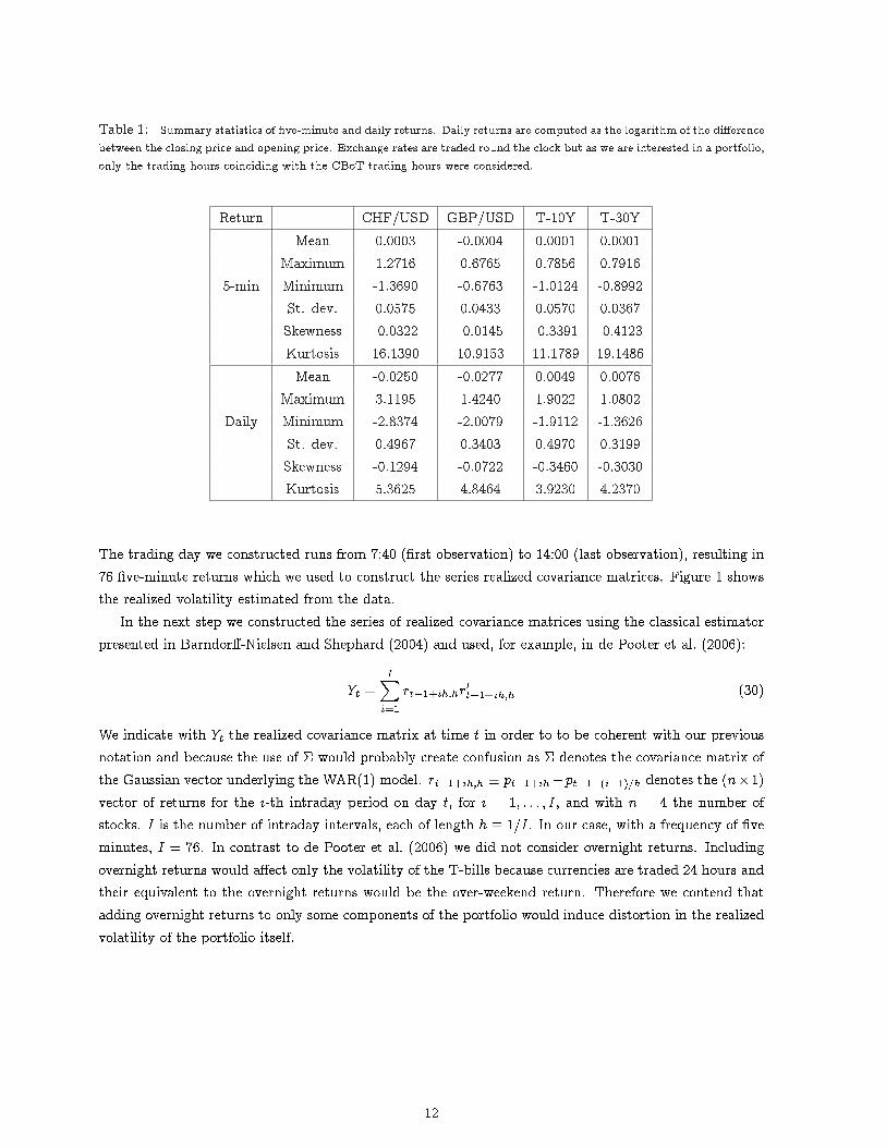
Table 1: Summary statistics of �ve-minute and daily returns. Daily returns are computed as the logarithm of the di�erencebetween the closing price and opening price. Exchange rates are traded round the clock but as we are interested in a portfolio,only the trading hours coinciding with the CBoT trading hours were considered.

Return CHF/USD GBP/USD T-10Y T-30YMean 0.0003 -0.0004 0.0001 0.0001

Maximum 1.2716 0.6765 0.7856 0.79165-min Minimum -1.3690 -0.6763 -1.0124 -0.8992

St. dev. 0.0575 0.0433 0.0570 0.0367Skewness -0.0322 -0.0145 -0.3391 -0.4123Kurtosis 16.1390 10.9153 11.1789 19.1486Mean -0.0250 -0.0277 0.0049 0.0076

Maximum 3.1195 1.4240 1.9022 1.0802Daily Minimum -2.8374 -2.0079 -1.9112 -1.3626

St. dev. 0.4967 0.3403 0.4970 0.3199Skewness -0.1294 -0.0722 -0.3460 -0.3030Kurtosis 5.3625 4.8464 3.9230 4.2370

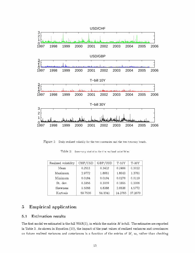
The trading day we constructed runs from 7:40 (�rst observation) to 14:00 (last observation), resulting in76 �ve-minute returns which we used to construct the series realized covariance matrices. Figure 1 showsthe realized volatility estimated from the data.

In the next step we constructed the series of realized covariance matrices using the classical estimatorpresented in Barndor�-Nielsen and Shephard (2004) and used, for example, in de Pooter et al. (2006):

Yt =IXi=1

rt�1+ih;hr0t�1+ih;h (30)

We indicate with Yt the realized covariance matrix at time t in order to to be coherent with our previousnotation and because the use of � would probably create confusion as � denotes the covariance matrix ofthe Gaussian vector underlying the WAR(1) model. rt�1+ih;h � pt�1+ih�pt�1+(i�1)=h denotes the (n�1)vector of returns for the i-th intraday period on day t, for i = 1; : : : ; I, and with n = 4 the number ofstocks. I is the number of intraday intervals, each of length h � 1=I. In our case, with a frequency of �veminutes, I = 76. In contrast to de Pooter et al. (2006) we did not consider overnight returns. Includingovernight returns would a�ect only the volatility of the T-bills because currencies are traded 24 hours andtheir equivalent to the overnight returns would be the over-weekend return. Therefore we contend thatadding overnight returns to only some components of the portfolio would induce distortion in the realizedvolatility of the portfolio itself.

12

1997 1998 1999 2000 2001 2002 2003 2004 2005 20060123

T−bill 10Y

1997 1998 1999 2000 2001 2002 2003 2004 2005 20060123

T−bill 30Y

1997 1998 1999 2000 2001 2002 2003 2004 2005 20060123

USD/CHF

1997 1998 1999 2000 2001 2002 2003 2004 2005 20060123

USD/GBP

Figure 1: Daily realized volatiliy for the two currencies and the two treasury bonds.

Table 2: Summary statistics for the realized volatilities

Realized volatility CHF/USD GBP/USD T-10Y T-30YMean 0.2511 0.1422 0.2466 0.1022

Maximum 2.9772 1.8661 1.8043 1.3761Minimum 0.0184 0.0164 0.0276 0.0119St. dev. 0.1856 0.1039 0.1895 0.1006Skewness 5.5066 4.8388 2.6636 4.5772Kurtosis 59.7536 54.3341 14.2783 37.2670

5 Empirical application

5.1 Estimation resultsThe �rst model we estimated is the full WAR(1), in which the matrixM is full. The estimates are reportedin Table 3. As shown in Equation (10), the impact of the past values of realized variances and covarianceson future realized variances and covariances is a function of the entries of M , so, rather than checking

13

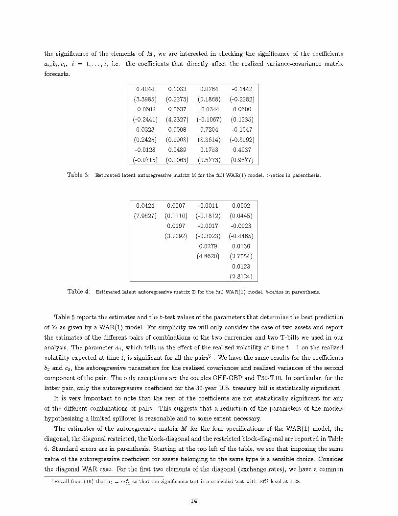
the signi�cance of the elements of M , we are interested in checking the signi�cance of the coe�cientsai; bi; ci; i = 1; : : : ; 3, i.e. the coe�cients that directly a�ect the realized variance-covariance matrixforecasts.

0.4044 0.1033 0.0764 -0.1442(3.3985) (0.2273) (0.1868) (-0.2282)-0.0602 0.5637 -0.0344 0.0600(-0.2441) (4.2327) (-0.1067) (0.1235)0.0323 0.0008 0.7204 -0.1047(0.2425) (0.0003) (3.3614) (-0.3092)-0.0128 0.0489 0.1753 0.4037(-0.0715) (0.2063) (0.5773) (0.9577)

Table 3: Estimated latent autoregressive matrix M for the full WAR(1) model. t-ratios in parenthesis.

0.0424 0.0007 -0.0011 0.0002(7.9627) (0.1110) (-0.1812) (0.0445)

0.0197 -0.0017 -0.0023(3.7092) (-0.3023) (-0.4465)

0.0279 0.0136(4.8620) (2.7554)

0.0123(2.8124)

Table 4: Estimated latent autoregressive matrix � for the full WAR(1) model. t-ratios in parenthesis.

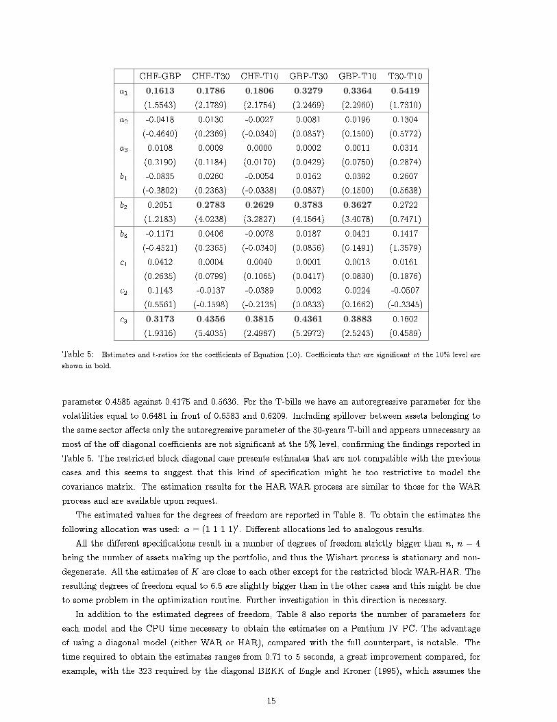
Table 5 reports the estimates and the t-test values of the parameters that determine the best predictionof Yt as given by a WAR(1) model. For simplicity we will only consider the case of two assets and reportthe estimates of the di�erent pairs of combinations of the two currencies and two T-bills we used in ouranalysis. The parameter a1, which tells us the e�ect of the realized volatility at time t� 1 on the realizedvolatility expected at time t, is signi�cant for all the pairs5 . We have the same results for the coe�cientsb2 and c3, the autoregressive parameters for the realized covariances and realized variances of the secondcomponent of the pair. The only exceptions are the couples CHF-GBP and T30-T10. In particular, for thelatter pair, only the autoregressive coe�cient for the 30-year U.S. treasury bill is statistically signi�cant.

It is very important to note that the rest of the coe�cients are not statistically signi�cant for anyof the di�erent combinations of pairs. This suggests that a reduction of the parameters of the modelshypothesizing a limited spillover is reasonable and to some extent necessary.

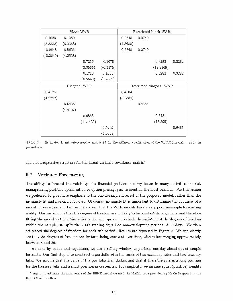
The estimates of the autoregressive matrix M for the four speci�cations of the WAR(1) model, thediagonal, the diagonal restricted, the block-diagonal and the restricted block-diagonal are reported in Table6. Standard errors are in parenthesis. Starting at the top left of the table, we see that imposing the samevalue of the autoregressive coe�cient for assets belonging to the same type is a sensible choice. Considerthe diagonal WAR case. For the �rst two elements of the diagonal (exchange rates), we have a common

5Recall from (10) that a1 = m211 so that the signi�cance test is a one-sided test with 10% level at 1.28.

14

CHF-GBP CHF-T30 CHF-T10 GBP-T30 GBP-T10 T30-T10a1 0:1613 0:1786 0:1806 0:3279 0:3364 0:5419

(1.5543) (2.1789) (2.1754) (2.2469) (2.2960) (1.7310)a2 -0.0418 0.0130 -0.0027 0.0081 0.0196 0.1304

(-0.4640) (0.2369) (-0.0340) (0.0857) (0.1500) (0.5772)a3 0.0108 0.0009 0.0000 0.0002 0.0011 0.0314

(0.2190) (0.1184) (0.0170) (0.0429) (0.0750) (0.2874)b1 -0.0835 0.0260 -0.0054 0.0162 0.0392 0.2607

(-0.3802) (0.2363) (-0.0338) (0.0857) (0.1500) (0.5638)b2 0.2051 0:2783 0:2629 0:3783 0:3627 0.2722

(1.2183) (4.0238) (3.2827) (4.1564) (3.4078) (0.7471)b3 -0.1171 0.0406 -0.0078 0.0187 0.0421 0.1417

(-0.4521) (0.2365) (-0.0340) (0.0856) (0.1491) (1.3579)c1 0.0412 0.0004 0.0040 0.0001 0.0013 0.0161

(0.2635) (0.0799) (0.1065) (0.0417) (0.0830) (0.1876)c2 0.1143 -0.0137 -0.0389 0.0062 0.0224 -0.0507

(0.5561) (-0.1598) (-0.2135) (0.0833) (0.1662) (-0.3345)c3 0:3173 0:4356 0:3815 0:4361 0:3883 0.1602

(1.9316) (5.4035) (2.4987) (5.2972) (2.5243) (0.4589)

Table 5: Estimates and t-ratios for the coe�cients of Equation (10). Coe�cients that are signi�cant at the 10% level areshown in bold.

parameter 0.4585 against 0.4175 and 0.5636. For the T-bills we have an autoregressive parameter for thevolatilities equal to 0.6481 in front of 0.6583 and 0.6209. Including spillover between assets belonging tothe same sector a�ects only the autoregressive parameter of the 30-years T-bill and appears unnecessary asmost of the o�-diagonal coe�cients are not signi�cant at the 5% level, con�rming the �ndings reported inTable 5. The restricted block diagonal case presents estimates that are not compatible with the previouscases and this seems to suggest that this kind of speci�cation might be too restrictive to model thecovariance matrix. The estimation results for the HAR-WAR process are similar to those for the WARprocess and are available upon request.

The estimated values for the degrees of freedom are reported in Table 8. To obtain the estimates thefollowing allocation was used: � = (1 1 1 1)0. Di�erent allocations led to analogous results.

All the di�erent speci�cations result in a number of degrees of freedom strictly bigger than n, n = 4being the number of assets making up the portfolio, and thus the Wishart process is stationary and non-degenerate. All the estimates of K are close to each other except for the restricted block WAR-HAR. Theresulting degrees of freedom equal to 6.5 are slightly bigger than in the other cases and this might be dueto some problem in the optimization routine. Further investigation in this direction is necessary.

In addition to the estimated degrees of freedom, Table 8 also reports the number of parameters foreach model and the CPU time necessary to obtain the estimates on a Pentium IV PC. The advantageof using a diagonal model (either WAR or HAR), compared with the full counterpart, is notable. Thetime required to obtain the estimates ranges from 0.71 to 5 seconds, a great improvement compared, forexample, with the 323 required by the diagonal BEKK of Engle and Kroner (1995), which assumes the

15

Block WAR Restricted block WAR0.4080 0.1060 0.2740 0.2740(3.5332) (0.2383) (4.8680)-0.0648 0.5626 0.2740 0.2740(-0.2649) (4.2528)

0.7216 -0.1078 0.3282 0.3282(3.3565) (-0.3175) (12.8269)0.1716 0.4035 0.3282 0.3282(0.5640) (0.9389)

Diagonal WAR Restricted diagonal WAR0.4175 0.4584(4.2792) (5.9889)

0.5636 0.4584(4.4107)

0.6583 0.6481(11.1432) (13.595)

0.6209 0.6481(6.0008)

Table 6: Estimated latent autoregressive matrix M for the di�erent speci�cation of the WAR(1) model. t-ratios inparenthesis.

same autoregressive structure for the latent variance-covariance matrix6.

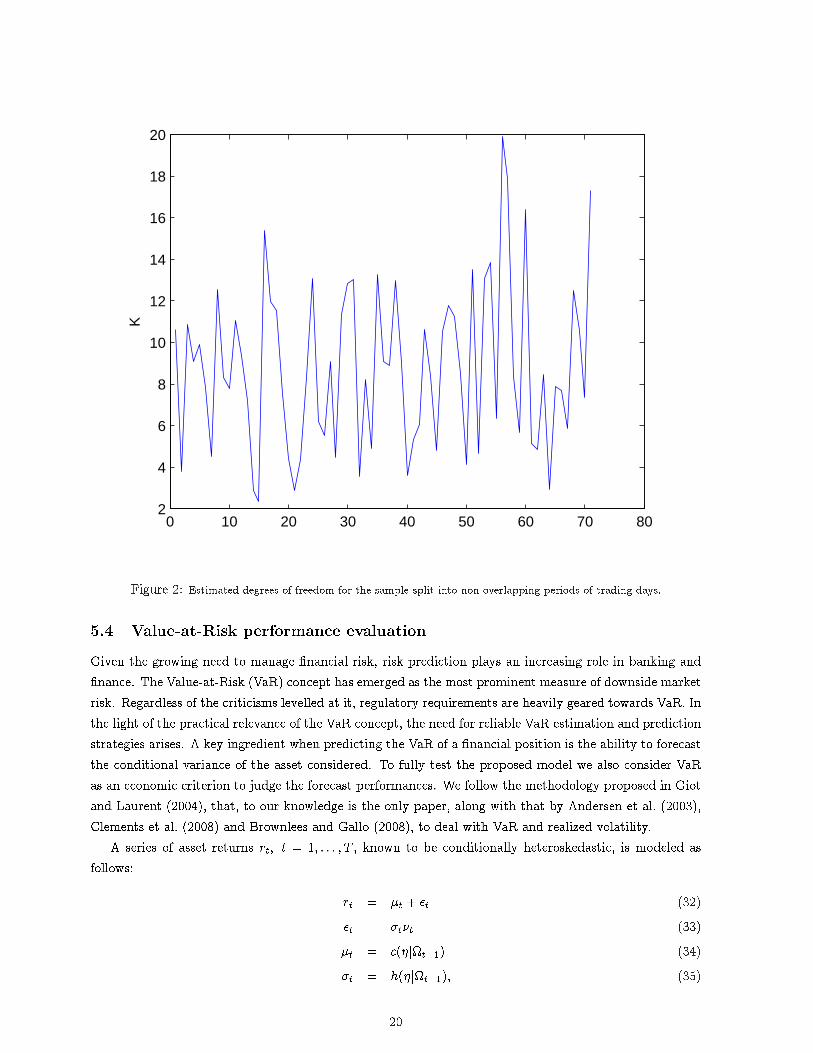
5.2 Variance ForecastingThe ability to forecast the volatility of a �nancial position is a key factor in many activities like riskmanagement, portfolio optimization or option pricing, just to mention the most common. For this reasonwe preferred to give more emphasis to the out-of-sample forecast of the proposed model, rather than thein-sample �t and in-sample forecast. Of course, in-sample �t is important to determine the goodness of amodel; however, unreported results showed that the WAR models have a very poor in-sample forecastingability. Our suspicion is that the degrees of freedom are unlikely to be constant through time, and therefore�tting the model to the entire series is not appropriate. To check the variation of the degrees of freedomwithin the sample, we split the 2,147 trading days into non-overlapping periods of 30 days. We thenestimated the degrees of freedom for each sub-period. Results are reported in Figure 2. We can clearlysee that the degrees of freedom are far form being constant over time, with values ranging approximatelybetween 3 and 20.

As done by banks and regulators, we use a rolling window to perform one-day-ahead out-of-sampleforecasts. Our �rst step is to construct a portfolio with the series of two exchange rates and two treasurybills. We assume that the value of the portfolio is in dollars and that it therefore carries a long positionfor the treasury bills and a short position in currencies. For simplicity, we assume equal (positive) weights

6 Again, to estimate the parameters of the BEKK model we used the Matlab code provided by Kevin Sheppard in theUCSD Garch toolbox.

16

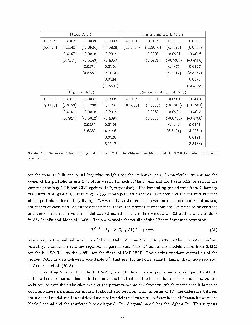
Block WAR Restricted block WAR0.0424 0.0007 -0.0002 -0.0003 0.0451 -0.0049 0.0000 0.0000(8.0529) (0.1140) (-0.0604) (-0.0828) (11.1560) (-1.2006) (0.0070) (0.0069)

0.0197 -0.0019 -0.0014 0.0228 -0.0024 -0.0016(3.7136) (-0.6149) (-0.4363) (5.6421) (-0.7805) (-0.4998)

0.0279 0.0136 0.0371 0.0127(4.8738) (2.7514) (9.9012) (3.3877)

0.0124 0.0076( 2.8801) ( 2.0225)

Diagonal WAR Restricted diagonal WAR0.0424 0.0011 -0.0004 -0.0004 0.0406 0.0011 -0.0004 -0.0004(8.1190) (0.3423) (-0.1238) (-0.1264) (8.5055) (0.3536) (-0.1201) (-0.1201)

0.0198 -0.0019 -0.0014 0.0230 -0.0021 -0.0015(3.7920) (-0.6012) (-0.4396) (6.1516) (-0.6732) (-0.4760)

0.0285 0.0154 0.0292 0.0151(5.6888) (4.2106) (6.6184) (4.2865)

0.0128 0.0121(3.1117) (3.5788)

Table 7: Estimated latent autoregressive matrix � for the di�erent speci�cation of the WAR(1) model. t-ratios inparenthesis.

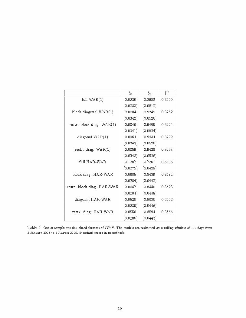
for the treasury bills and equal (negative) weights for the exchange rates. In particular, we assume theowner of the portfolio invests 0.75 of his wealth for each of the T-bills and short-sells 0.25 for each of thecurrencies to buy CHF and GBP against USD, respectively. The forecasting period runs from 2 January2003 until 8 August 2005, resulting in 653 one-step-ahead forecasts. For each day the realized varianceof the portfolio is forecast by �tting a WAR model to the series of covariance matrices and re-estimatingthe model at each step. As already mentioned above, the degrees of freedom are likely not to be constantand therefore at each step the model was estimated using a rolling window of 100 trading days, as donein Aït-Sahalia and Mancini (2008). Table 9 presents the results of the Mincer-Zarnowitz regression:

IV 1=2t = b0 + b1Et�1[RVt]1=2 + error; (31)

where IVt is the realized volatility of the portfolio at time t and Et�1[RVt] is the forecasted realizedvolatility. Standard errors are reported in parenthesis. The R2 across the models varies from 0.3209for the full WAR(1) to the 0.3655 for the diagonal HAR-WAR. The moving windows estimation of thevarious WAR models delivered acceptable R2, that are, for instance, slightly higher than those reportedin Andersen et al. (2003).

It interesting to note that the full WAR(1) model has a worse performance if compared with itsrestricted counterparts. This might be due to the fact that the the full model is not the most appropriateas it carries over the estimation error of the parameters into the forecasts, which means that it is not asgood as a more parsimonious model. It should also be noted that, in terms of R2, the di�erence betweenthe diagonal model and the restricted diagonal model is not relevant. Neither is the di�erence between theblock diagonal and the restricted block diagonal. The diagonal model has the highest R2. This suggests

17

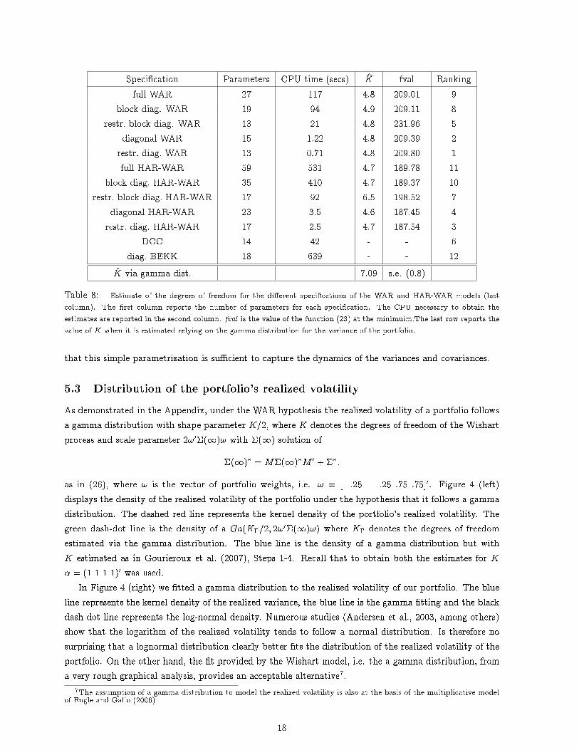
Speci�cation Parameters CPU time (secs) K̂ fval Rankingfull WAR 27 117 4.8 209.01 9

block diag. WAR 19 94 4.9 209.11 8restr. block diag. WAR 13 21 4.8 231.96 5

diagonal WAR 15 1.22 4.8 209.39 2restr. diag. WAR 13 0.71 4.8 209.80 1full HAR-WAR 59 531 4.7 189.78 11

block diag. HAR-WAR 35 410 4.7 189.37 10restr. block diag. HAR-WAR 17 92 6.5 198.52 7

diagonal HAR-WAR 23 3.5 4.6 187.45 4restr. diag. HAR-WAR 17 2.5 4.7 187.54 3

DCC 14 42 - - 6diag. BEKK 18 639 - - 12

K̂ via gamma dist. 7.09 s.e. (0.8)

Table 8: Estimate of the degrees of freedom for the di�erent speci�cations of the WAR and HAR-WAR models (lastcolumn). The �rst column reports the number of parameters for each speci�cation. The CPU necessary to obtain theestimates are reported in the second column. fval is the value of the function (23) at the minimuim.The last row reports thevalue of K when it is estimated relying on the gamma distribution for the variance of the portfolio.

that this simple parametrization is su�cient to capture the dynamics of the variances and covariances.

5.3 Distribution of the portfolio's realized volatilityAs demonstrated in the Appendix, under the WAR hypothesis the realized volatility of a portfolio followsa gamma distribution with shape parameter K=2, where K denotes the degrees of freedom of the Wishartprocess and scale parameter 2!0�(1)! with �(1) solution of

�(1)� = M�(1)�M 0 + ��:

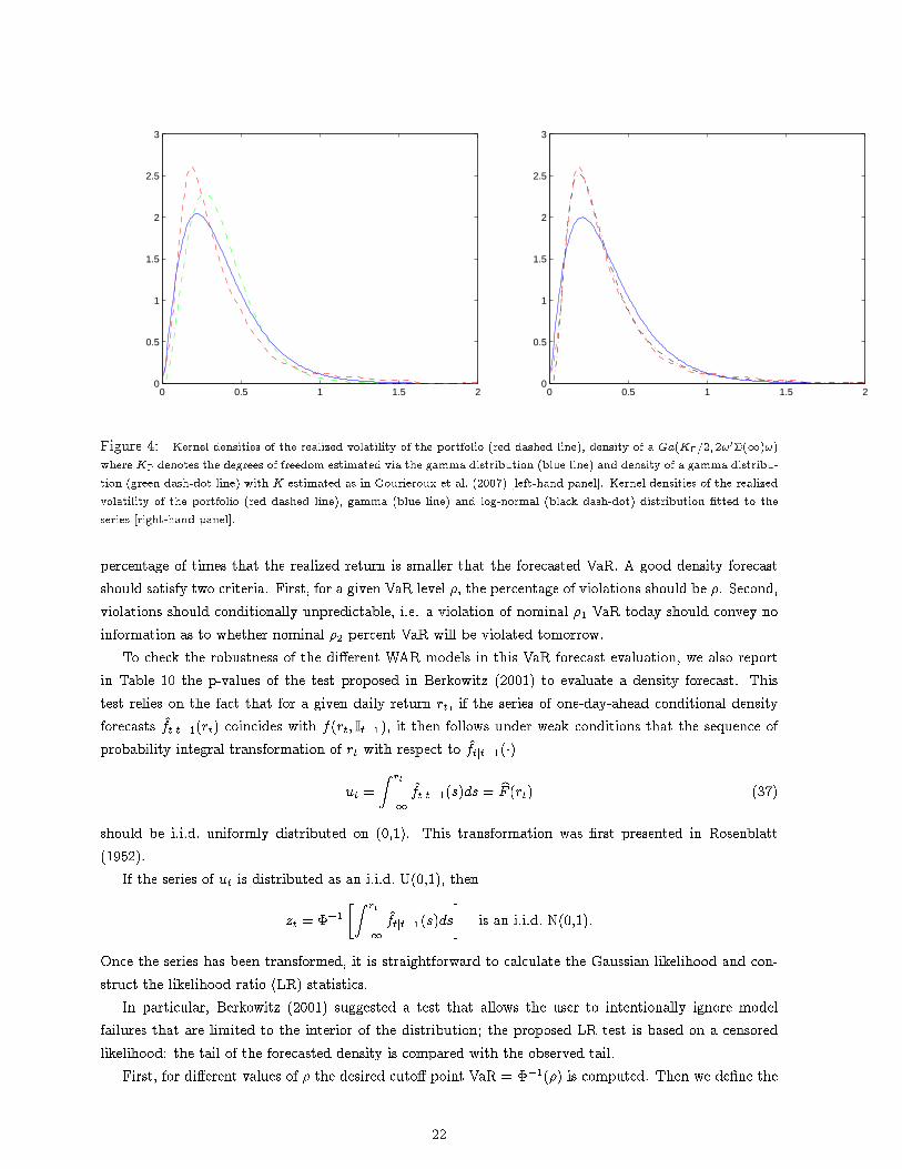
as in (26), where ! is the vector of portfolio weights, i.e. ! = [�:25 � :25 :75 :75]0. Figure 4 (left)displays the density of the realized volatility of the portfolio under the hypothesis that it follows a gammadistribution. The dashed red line represents the kernel density of the portfolio's realized volatility. Thegreen dash-dot line is the density of a Ga(K�=2; 2!0�(1)!) where K� denotes the degrees of freedomestimated via the gamma distribution. The blue line is the density of a gamma distribution but withK estimated as in Gourieroux et al. (2007), Steps 1-4. Recall that to obtain both the estimates for K� = (1 1 1 1)0 was used.

In Figure 4 (right) we �tted a gamma distribution to the realized volatility of our portfolio. The blueline represents the kernel density of the realized variance, the blue line is the gamma �tting and the blackdash dot line represents the log-normal density. Numerous studies (Andersen et al., 2003, among others)show that the logarithm of the realized volatility tends to follow a normal distribution. Is therefore nosurprising that a lognormal distribution clearly better �ts the distribution of the realized volatility of theportfolio. On the other hand, the �t provided by the Wishart model, i.e. the a gamma distribution, froma very rough graphical analysis, provides an acceptable alternative7.

7The assumption of a gamma distribution to model the realized volatility is also at the basis of the multiplicative modelof Engle and Gallo (2006)

18

b0 b1 R2

full WAR(1) 0.0226 0.8988 0.3209(0.0333) (0.0512)

block diagonal WAR(1) 0.0004 0.9349 0.3262(0.0342) (0.0526)

restr. block diag. WAR(1) 0.0046 0.9405 0.3224(0.0341) (0.0524)

diagonal WAR(1) 0.0064 0.9434 0.3299(0.0343) (0.0526)

restr. diag. WAR(1) 0.0059 0.9428 0.3298(0.0342) (0.0526)

full HAR-WAR 0.1387 0.7361 0.3103(0.0275) (0.0429)

block diag. HAR-WAR 0.0685 0.8439 0.3584(0.0284) (0.0442)

restr. block diag. HAR-WAR 0.0647 0.8440 0.3623(0.0284) (0.0438)

diagonal HAR-WAR 0.0520 0.8630 0.3662(0.0289) (0.0446)

restr. diag. HAR-WAR 0.0550 0.8594 0.3655(0.0286) (0.0443)

Table 9: Out-of-sample one-day-ahead forecast of IV 1=2. The models are estimated on a rolling window of 100 days from2 January 2003 to 8 August 2005. Standard errors in parenthesis.

19

0 10 20 30 40 50 60 70 802

4

6

8

10

12

14

16

18

20K

Figure 2: Estimated degrees of freedom for the sample split into non-overlapping periods of trading days.

5.4 Value-at-Risk performance evaluationGiven the growing need to manage �nancial risk, risk prediction plays an increasing role in banking and�nance. The Value-at-Risk (VaR) concept has emerged as the most prominent measure of downside marketrisk. Regardless of the criticisms levelled at it, regulatory requirements are heavily geared towards VaR. Inthe light of the practical relevance of the VaR concept, the need for reliable VaR estimation and predictionstrategies arises. A key ingredient when predicting the VaR of a �nancial position is the ability to forecastthe conditional variance of the asset considered. To fully test the proposed model we also consider VaRas an economic criterion to judge the forecast performances. We follow the methodology proposed in Giotand Laurent (2004), that, to our knowledge is the only paper, along with that by Andersen et al. (2003),Clements et al. (2008) and Brownlees and Gallo (2008), to deal with VaR and realized volatility.

A series of asset returns rt; t = 1; : : : ; T , known to be conditionally heteroskedastic, is modeled asfollows:

rt = �t + �t (32)�t = �t�t (33)�t = c(�jt�1) (34)�t = h(�jt�1); (35)

20

0 100 200 300 400 500 600 7000

0.5

1

1.5

2

2.5

3

3.5

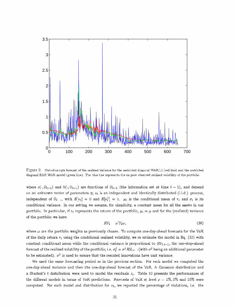
Figure 3: Out-of-sample forecast of the realized variance for the restricted diagonal WAR(1) (red line) and the restricteddiagonal HAR-WAR model (green line). The blue line represents the ex-post observed realized volatility of the portfolio.

where c(�;t�1) and h(�;t�1) are functions of t�1 (the information set at time t � 1), and dependon an unknown vector of parameters �; �t is an independent and identically distributed (i.i.d.) process,independent of t�1, with E[�t] = 0 and E[�2

t ] = 1. �t is the conditional mean of rt and �t is itsconditional variance. In our setting we assume, for simplicity, a constant mean for all the assets in ourportfolio. In particular, if rt represents the return of the portfolio, �t = � and for the (realized) varianceof the portfolio we have:

RVt = !0Yt!; (36)

where ! are the portfolio weights as previously chosen. To compute one-day-ahead forecasts for the VaRof the daily return rt using the conditional realized volatility, we re-estimate the model in Eq. (32) withconstant conditional mean while the conditional variance is proportional to RVtjt�1, the one-step-aheadforecast of the realized volatility of the portfolio; i.e. �2

t = �2RVtjt�1(with �2 being an additional parameterto be estimated). �2 is used to ensure that the rescaled innovations have unit variance.

We used the same forecasting period as in the previous section. For each model we computed theone-day-ahead variance and then the one-day-ahead forecast of the VaR. A Gaussian distribution anda Student's t distribution were used to model the residuals zt. Table 10 presents the performances ofthe di�erent models in terms of VaR predictions. Forecasts of VaR at level � = 1%; 5% and 10% werecomputed. For each model and distribution for �t, we reported the percentage of violations, i.e. the

21

0 0.5 1 1.5 20

0.5

1

1.5

2

2.5

3

0 0.5 1 1.5 20

0.5

1

1.5

2

2.5

3

Figure 4: Kernel densities of the realized volatility of the portfolio (red dashed line), density of a Ga(K�=2; 2!0�(1)!)where K� denotes the degrees of freedom estimated via the gamma distribution (blue line) and density of a gamma distribu-tion (green dash-dot line) with K estimated as in Gourieroux et al. (2007) [left-hand panel]. Kernel densities of the realizedvolatility of the portfolio (red dashed line), gamma (blue line) and log-normal (black dash-dot) distribution �tted to theseries [right-hand panel].

percentage of times that the realized return is smaller that the forecasted VaR. A good density forecastshould satisfy two criteria. First, for a given VaR level �, the percentage of violations should be �. Second,violations should conditionally unpredictable, i.e. a violation of nominal �1 VaR today should convey noinformation as to whether nominal �2 percent VaR will be violated tomorrow.

To check the robustness of the di�erent WAR models in this VaR forecast evaluation, we also reportin Table 10 the p-values of the test proposed in Berkowitz (2001) to evaluate a density forecast. Thistest relies on the fact that for a given daily return rt, if the series of one-day-ahead conditional densityforecasts f̂tjt�1(rt) coincides with f(rt; It�1), it then follows under weak conditions that the sequence ofprobability integral transformation of rt with respect to f̂tjt�1(�)

ut =Z rt

�1f̂tjt�1(s)ds = bF (rt) (37)

should be i.i.d. uniformly distributed on (0,1). This transformation was �rst presented in Rosenblatt(1952).

If the series of ut is distributed as an i.i.d. U(0,1), then

zt = ��1�Z rt

�1f̂tjt�1(s)ds

�is an i.i.d. N(0,1).

Once the series has been transformed, it is straightforward to calculate the Gaussian likelihood and con-struct the likelihood ratio (LR) statistics.

In particular, Berkowitz (2001) suggested a test that allows the user to intentionally ignore modelfailures that are limited to the interior of the distribution; the proposed LR test is based on a censoredlikelihood: the tail of the forecasted density is compared with the observed tail.

First, for di�erent values of � the desired cuto� point VaR = ��1(�) is computed. Then we de�ne the

22

new variable of interest as

z�t =

(VaR if zt � VaRzz if zt < VaR:

The log-likelihood function for joint estimation of � and �2 is

L(�; �jz�) =X

z�<V aRlog

1���z�t � ��

�+

Xz�=V aR

log�

1� ��V aR� �

�

��(38)

=X

z�<V aR

��1

2log(2��2)� 1

2�(z�t � �)2

�+

Xz�=V aR

log�

1� ��V aR� �

�

��: (39)

To construct the LR test the null hypothesis requires that � = 0, �2 = 1. Therefore the restrictedlikelihood L(0,1) is compared to the unrestricted one, L(�̂; �̂2). The test statistic is then

LRtail = �2(L(0; 1)� L(�̂; �̂2)) (40)

Under the null hypothesis, the test statistic is distributed �2(2).

[Table 10 somewhere here]

Table 10 reports, for the di�erent models considered and di�erent assumptions for the residuals, thepercentage of violations along with the p-value of the Berkowitz's test.

The relative number of violations is close to the theoretical one and assuming a t distribution for theresiduals does not really improve the forecasting performances. For all the proposed speci�cations of theWAR model, the Berkowitz test does not reject the null hypothesis of appropriateness of the forecasteddensities. Therefore all the models provide acceptable VaR forecasts. For the 1% VaR level, the results aresomewhat surprising. The percentage of VaR violations is, for all the speci�cations, around 2.4% in frontof a theoretical value of 1%. However, the p-values of the Berkowitz test are all higher than the rejectionthreshold of, say, 5%. This might be explained by the fact that the test proposed by Berkowitz is not apointwise evaluation of the VaR violations, but rather analyzes the entire forecasted densities, or, in ourcase, the left tail of the distribution.

Besides the good forecasting performances of the proposed models, we want to stress the fact thatthere is no notable di�erence in the forecasting ability of the di�erent speci�cations. Therefore, a veryparsimonious (and thus quick to estimate) model like the restricted diagonal WAR is su�cient to modelthe riskiness of our portfolio.

6 Conclusions and direction for future researchIn this paper we proposed a particular set of restricted speci�cation of the WAR model for realized(co)variances. Our speci�cations rely on the ability to group assets according to some criterion, for examplethe economic sector, a common feature in the variance-covariance dynamics, and so on. This allowed us todrastically reduce the number of parameters. A comparison between the di�erent speci�cations highlightedthat there is no loss when a more parsimonious model is chosen. This is essentially due to the fact thatthe restricted model was justi�ed by the data.

However, some aspects of the WAR process need to be clari�ed. In particular, the degrees of freedomseem to vary through time and it is not clear by which variables they are driven.

23

A straightforward extension of the present work involves applaying the WAR model to solve concrete�nancial problems like dynamic portfolio choice, for instance.

This and other applications of the WAR model are left for future research.

ReferencesAït-Sahalia, Y. and L. Mancini (2008): �Out of sample forecast of quadratic variation,� Journal ofEconometrics, forthcoming.

Andersen, T. and T. Bollerslev (1997): �Heterogeneous information arrivals and return volatiliydynamics: Uncovering the long run in high frequency data,� The Journal of Finance, 52, 975�1005.

��� (1998): �Answering the skeptics: Yes, standard volatility models do provide accurate forecasts,�International Economic Review, 39, 885�905.

Andersen, T., T. Bollerslev, F. Diebold, and H. Ebens (2001a): �The distribution of realizedstock return volatility,� Journal of Financial Economics, 43�76.

Andersen, T., T. Bollerslev, F. Diebold, and P. Labys (2001b): �The distribution of realizedexchange rate volatility,� Journal of the American Statistical Association, 96, 42�55.

��� (2003): �Modeling and forecasting realized volatility,� Econometrica, 71, 579�625.

Andreou, E. and E. Ghysels (2002): �Rolling sample volatility estimators: some new theoretical,simulation and empirical results,� Journal of Business and Economic Statistics, 20, 363�376.

Asai, M., M. Caporin, and M. McAleer (2008): �Block structure multivariate stochastic volatility,�Manuscript.

Bandi, F. and J. Russel (2005): �Realized covariation, realized beta and microstructure noise,� unpub-lished paper.

Bandi, F., J. Russel, and Y. Zhu (2006): �Using high-frequency data in dynamic portfolio choice,�Econometric Reviews, forthcoming.

Barndorff-Nielsen, O. and N. Shephard (2004): �Econometric analysis of realized covariation: high-frequency based covariance, regressions, and correlation in �nancial economics,� Econometrica, 72,885�925.

Bauer, G. and K. Vorkink (2007): �Multivariate realized stock market volatility,� Bank of CanadaWorking Papers 2007-20.

Berkowitz, J. (2001): �Testing densities forecasts, with applications to risk management,� Journal ofBusiness and Economic Statistics, 19, 465�474.

Billio, M. and M. Caporin (2008): �A generalised dynamic conditional correlation model for portfoliorisk evaluation,� Mathematics and Computers in Simulations, forthcoming.

Billio, M., M. Caporin, and M. Gobbo (2006): �Flexible dynamic conditional correlation multivariateGARCH for asset allocation,� Applied Financial Economics Letters, 2, 123�130.

24

Bonato, M. (2008): �Estimating the degrees of freedom of the realized volatility Wishart autoregressivemodel,� Manuscript.

Brownlees, C. and G. Gallo (2008): �Comparison of Volatility Measures: A Risk Management Per-spective,� .

Caporin, M. and P. Paruolo (2008): �Spatial dependence in multivariate volatility models,� WorkingPaper.

Chiriac, R. (2007): �Nonstationary Wishart autoregressive model,� Working Paper.

Chiriac, R. and V. Voev (2008): �Modelling and forecasting multivariate realized volatility,� WorkingPaper.

Clements, M. P., A. B. Galvao, and J. H. Kim (2008): �Quantile forecasts of daily exchange ratesreturns from forecasts of realized volatility,� Journal of Empirical Finance, 15, 729�750.

Corsi, F. (2004): �A simple long memory model of realized volatility,� Tech. Report, University ofSouthern Switzerland.

Corsi, F., U. Kretschmer, S. Mittnik, and C. Pigorsch (2007): �The volatility of realized volatility,�Journal of Financial Econometrics, 27, 46�78.

de Pooter, M., M. Martens, and D. van Dijk (2006): �Predicting the daily covariance matrix for S&P100 stocks using intraday data - But which frequency to use?� Econometric Reviews, forthcoming.

Engle, R. (2002): �Dynamic conditional correlation - a simple class of multivariate GARCH models,�Journal of Business and Economic Statistics, 20, 339�350.

Engle, R. and G. Gallo (2006): �A Multiple Indicators Model for Volatility Using Intra-Daily Data,�Journal of Econometrics, 131, 3�27.

Engle, R. and B. Kelly (2008): �Dynamic Equicorrelations,� Working Paper.

Engle, R. F. and F. K. Kroner (1995): �Multivarariate simultaneous generalized ARCH,� EconometricTheory, 11, 122�150.

Fleming, J., C. Kirby, and B. Ostdiek (2001): �The economic value of volatility,� Journal of Finance,56, 329�352.

��� (2003): �The economic value of volatility timing using `realized' volatiltiy,� Journal of FinancialEconomics, 67, 473�509.

Foster, D. and D. Nelson (1996): �Continuous record asymptotics for rolling sample variance estima-tors,� Econometrica, 64, 139�174.

Gallant, R., C. Hsu, and G. Tauchen (1999): �Using daily range data to calibrate volatitliy di�usionsand extract the forward integrated variance,� The Review of Economics and Statistics, 81, 617�631.

Giot, P. and S. Laurent (2004): �Modeling daily Value-at-Risk using realized volatiltiy and ARCHtype models,� Journal of Empirical Finance, 11, 379�398.

25

Gourieroux, C. (2007): �Positivity conditions for a bivariate autoregressive volatility speci�cations,�Journal of Financial Econometrics, 5, 624�636.

Gourieroux, C., J. Jasiak, and R. Sufana (2007): �The Wishart autoregressive process of multivariatestochastic volatility,� Journal of Econometrics, forthcoming.

Granger, C. (1980): �Long memory relationships and the aggregation of dynamic models,� Journal ofEconometrics, 14, 227�238.

Hayashi, T. and N. Yoshida (2005): �On covariance estimation of non-synchronously observed di�usionprocesses,� Bernoulli, 11, 359�379.

��� (2006): �Estimating correlations with nonsynchronous observations in continuous di�usion models,�Working Paper.

LeBaron, B. (2001): �Stochastic volatility as a simple generator of �nancial power-laws and long memory,�Quantitative Finance, 1, 621 � 631.

Martens, M. and D. van Dijk (2007): �Measuring volatility with the realized range,� Journal ofEconometrics, 181�207.

McAleer, M. and M. Medeiros (2006): �Realized volatility: a review,� Working Paper.

Meucci, A. (2005): Risk and asset allocation, Springer.

Müller, U., M. Dacorogna, R. Dave, R. Olsen, R. Piquet, and J. von Weizsäcker (1997):�Volatilities of di�erent time resolutions - Analyzing the dynamics of market components,� Journal ofEmpirical Finance, 4, 213�239.

Müller, U., M. Dacorogna, R. Dave, O. Pictet, R. Olsen, and J. Ward (1993): �Fractals andintrinsic time - a challenge to econometricians,� XXXIX International AEA Conference on RealTime Econometris, 14-15 Oct 1993, Luxembourg.

Pong, S., M. Shackleton, S. Taylor, and X. Xu (2004): �Forecasting currency volatility: A compar-ison of implied volatilities and AR(FI)MA models,� Journal of Banking and Finance, 28, 2514�2563.

Rosenblatt, M. (1952): �Remarks on a multivariate transformation,� The Annals of MathematicalStatistics, 23, 470�472.

Sheppard, K. (2006): �Realized covariance and scrambling,� Manuscript.

Thomakos, D. and T. Wang (2003): �Realized volatility in the futures markets,� Journal of EmpiricalFianance, 321�353.

Zhang, L. (2006): �Estimating covariation: Epps e�ect, microstructure noise.� Working Paper.

26

A Appendix

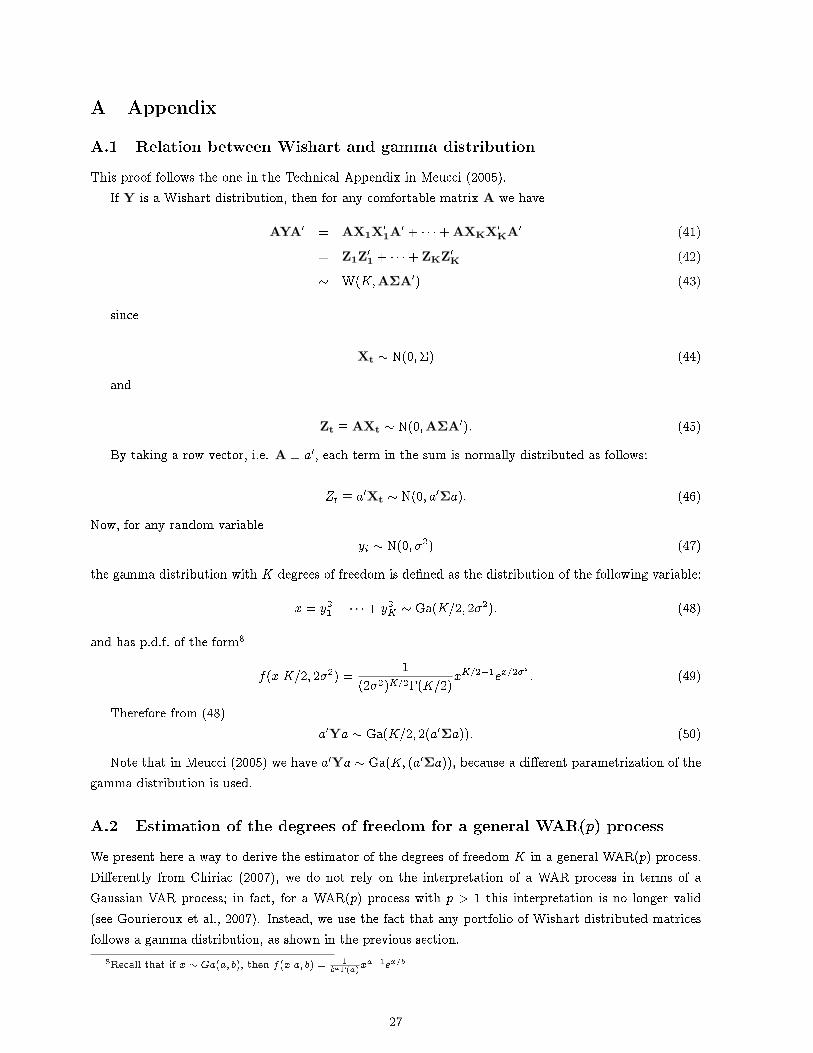
A.1 Relation between Wishart and gamma distributionThis proof follows the one in the Technical Appendix in Meucci (2005).

If Y is a Wishart distribution, then for any comfortable matrix A we have

AYA0 = AX1X01A0 + � � �+ AXKX0KA0 (41)= Z1Z01 + � � �+ ZKZ0K (42)� W(K;AΣA0) (43)

since

Xt � N(0;�) (44)

and

Zt � AXt � N(0;AΣA0): (45)

By taking a row vector, i.e. A � a0, each term in the sum is normally distributed as follows:

Zt � a0Xt � N(0; a0Σa): (46)

Now, for any random variableyi � N(0; �2) (47)

the gamma distribution with K degrees of freedom is de�ned as the distribution of the following variable:

x = y21 + � � �+ y2

K � Ga(K=2; 2�2): (48)

and has p.d.f. of the form8

f(xjK=2; 2�2) =1

(2�2)K=2�(K=2)xK=2�1ex=2�

s: (49)

Therefore from (48)a0Ya � Ga(K=2; 2(a0Σa)): (50)

Note that in Meucci (2005) we have a0Ya � Ga(K; (a0Σa)), because a di�erent parametrization of thegamma distribution is used.

A.2 Estimation of the degrees of freedom for a general WAR(p) processWe present here a way to derive the estimator of the degrees of freedom K in a general WAR(p) process.Di�erently from Chiriac (2007), we do not rely on the interpretation of a WAR process in terms of aGaussian VAR process; in fact, for a WAR(p) process with p > 1 this interpretation is no longer valid(see Gourieroux et al., 2007). Instead, we use the fact that any portfolio of Wishart-distributed matricesfollows a gamma distribution, as shown in the previous section.

8Recall that if x � Ga(a; b), then f(xja; b) = 1ba�(a)x

a�1ex=b

27

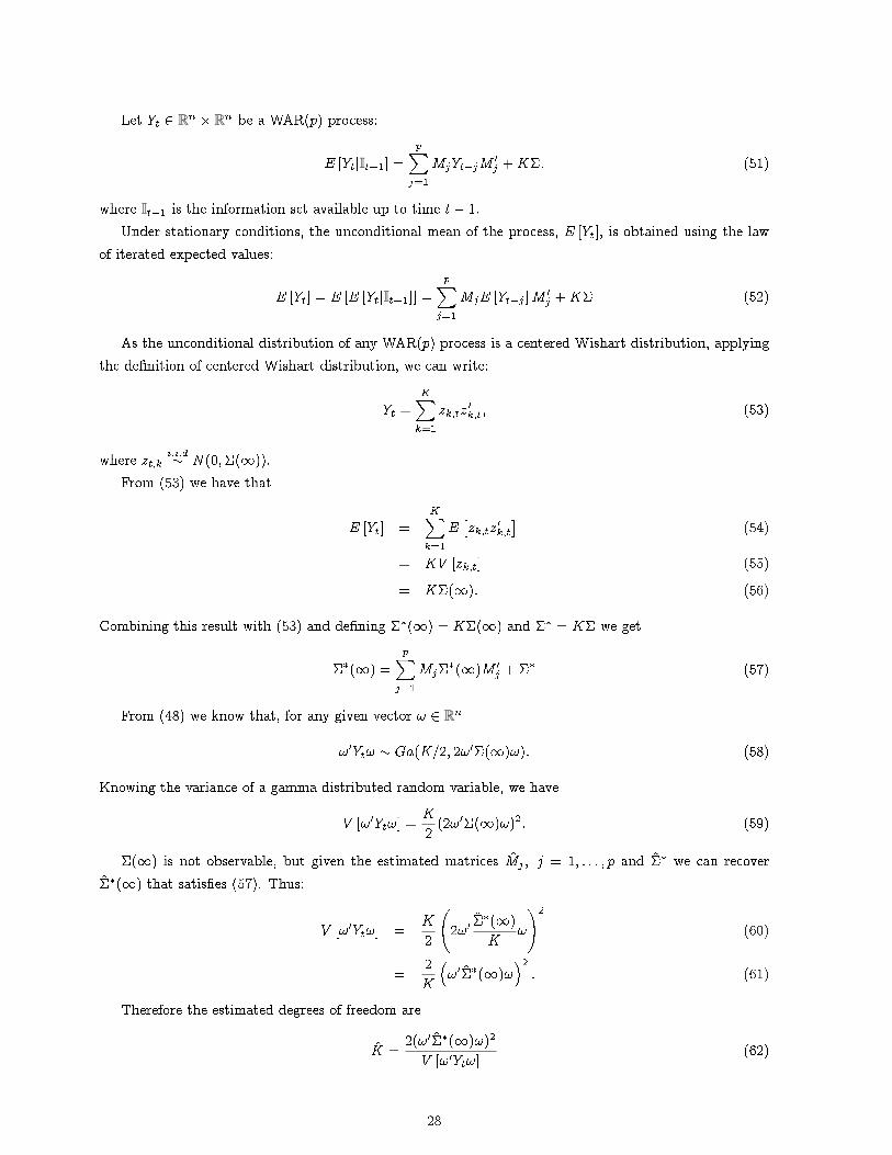
Let Yt 2 Rn � Rn be a WAR(p) process:

E [YtjIt�1] =pXj=1

MjYt�jM 0j +K�: (51)

where It�1 is the information set available up to time t� 1.Under stationary conditions, the unconditional mean of the process, E [Yt], is obtained using the law

of iterated expected values:

E [Yt] = E [E [YtjIt�1]] =pXj=1

MjE [Yt�j ]M 0j +K� (52)

As the unconditional distribution of any WAR(p) process is a centered Wishart distribution, applyingthe de�nition of centered Wishart distribution, we can write:

Yt =KXk=1

zk;tz0k;t; (53)

where zt;k i:i:d� N(0;�(1)).From (53) we have that

E [Yt] =KXk=1

E�zk;tz0k;t

�(54)

= KV [zk;t] (55)= K�(1): (56)

Combining this result with (53) and de�ning ��(1) = K�(1) and �� = K� we get

��(1) =pXj=1

Mj��(1)M 0j + �� (57)

From (48) we know that, for any given vector ! 2 Rn

!0Yt! � Ga(K=2; 2!0�(1)!): (58)

Knowing the variance of a gamma-distributed random variable, we have

V [!0Yt!] =K2

(2!0�(1)!)2: (59)

�(1) is not observable, but given the estimated matrices M̂j ; j = 1; : : : ; p and �̂� we can recover�̂�(1) that satis�es (57). Thus:

V [!0Yt!] =K2

2!0 �̂

�(1)K

!

!2

(60)

=2K

�!0�̂�(1)!

�2: (61)

Therefore the estimated degrees of freedom are

K̂ =2(!0�̂�(1)!)2

V [!0Yt!](62)

28

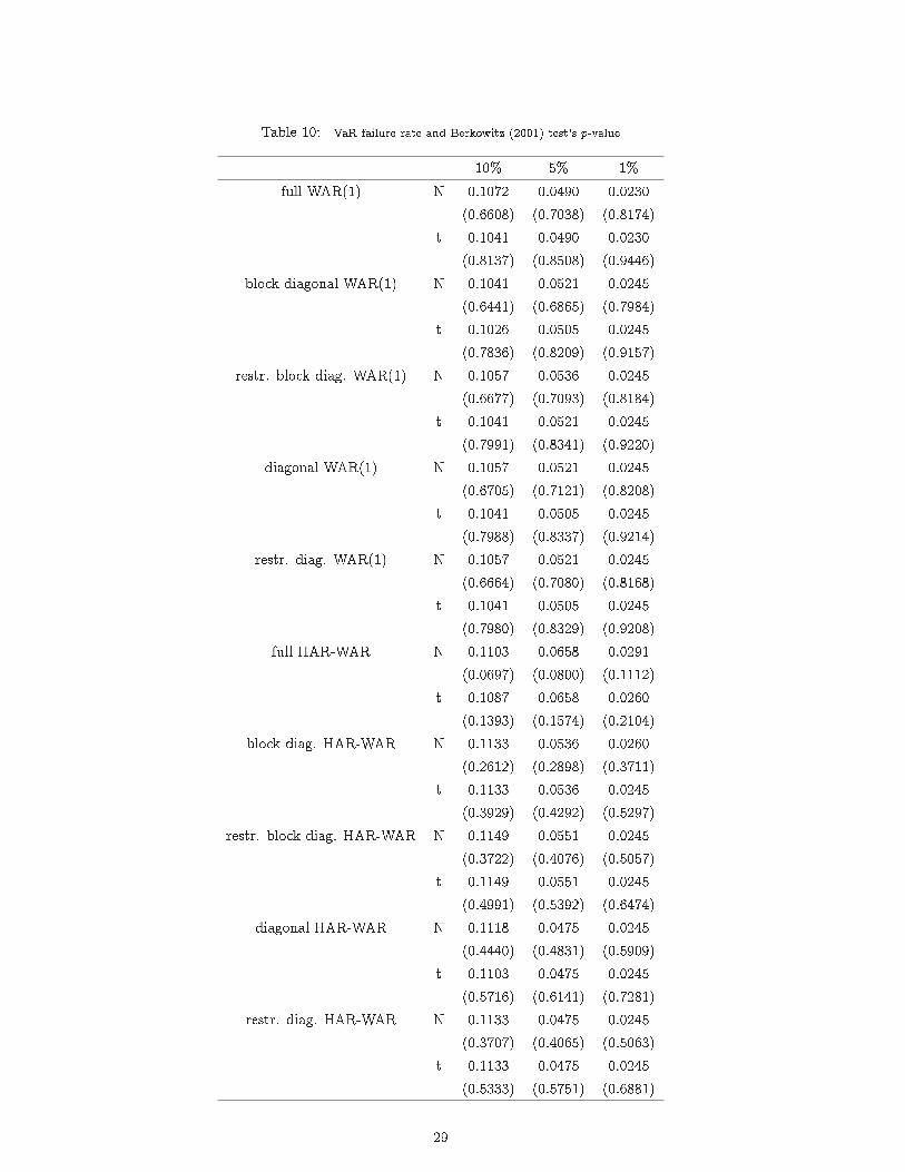
Table 10: VaR failure rate and Berkowitz (2001) test's p-value

10% 5% 1%full WAR(1) N 0.1072 0.0490 0.0230

(0.6608) (0.7038) (0.8174)t 0.1041 0.0490 0.0230

(0.8137) (0.8508) (0.9446)block diagonal WAR(1) N 0.1041 0.0521 0.0245

(0.6441) (0.6865) (0.7984)t 0.1026 0.0505 0.0245

(0.7836) (0.8209) (0.9157)restr. block diag. WAR(1) N 0.1057 0.0536 0.0245

(0.6677) (0.7093) (0.8184)t 0.1041 0.0521 0.0245

(0.7991) (0.8341) (0.9220)diagonal WAR(1) N 0.1057 0.0521 0.0245

(0.6705) (0.7121) (0.8208)t 0.1041 0.0505 0.0245

(0.7988) (0.8337) (0.9214)restr. diag. WAR(1) N 0.1057 0.0521 0.0245

(0.6664) (0.7080) (0.8168)t 0.1041 0.0505 0.0245

(0.7980) (0.8329) (0.9208)full HAR-WAR N 0.1103 0.0658 0.0291

(0.0697) (0.0800) (0.1112)t 0.1087 0.0658 0.0260

(0.1393) (0.1574) (0.2104)block diag. HAR-WAR N 0.1133 0.0536 0.0260

(0.2612) (0.2898) (0.3711)t 0.1133 0.0536 0.0245

(0.3929) (0.4292) (0.5297)restr. block diag. HAR-WAR N 0.1149 0.0551 0.0245

(0.3722) (0.4076) (0.5057)t 0.1149 0.0551 0.0245

(0.4991) (0.5392) (0.6474)diagonal HAR-WAR N 0.1118 0.0475 0.0245

(0.4440) (0.4831) (0.5909)t 0.1103 0.0475 0.0245

(0.5716) (0.6141) (0.7281)restr. diag. HAR-WAR N 0.1133 0.0475 0.0245

(0.3707) (0.4065) (0.5063)t 0.1133 0.0475 0.0245

(0.5333) (0.5751) (0.6881)

29