Department of Economics and Business Economics

Aarhus University

Fuglesangs Allé 4

DK-8210 Aarhus V

Denmark

Email: oekonomi@au.dk

Tel: +45 8716 5515

Forecasting daily political opinion polls using the fractionally

cointegrated VAR model

Morten Ørregaard Nielsen and Sergei S. Shibaev

CREATES Research Paper 2016-30

Forecasting daily political opinion polls using thefractionally cointegrated VAR model∗

Morten Ørregaard Nielsen†

Queen’s University and CREATESSergei S. Shibaev

Queen’s University

September 22, 2016

Abstract

We examine forecasting performance of the recent fractionally cointegrated vectorautoregressive (FCVAR) model. We use daily polling data of political support inthe United Kingdom for 2010-2015 and compare with popular competing models atseveral forecast horizons. Our findings show that the four variants of the FCVARmodel considered are generally ranked as the top four models in terms of forecastaccuracy, and the FCVAR model significantly outperforms both univariate fractionalmodels and the standard cointegrated VAR (CVAR) model at all forecast horizons.The relative forecast improvement is higher at longer forecast horizons, where the rootmean squared forecast error of the FCVAR model is up to 15% lower than that ofthe univariate fractional models and up to 20% lower than that of the CVAR model.In an empirical application to the 2015 UK general election, the estimated commonstochastic trend from the model follows the vote share of the UKIP very closely, andwe thus interpret it as a measure of Euro-skepticism in public opinion rather than anindicator of the more traditional left-right political spectrum. In terms of prediction ofvote shares in the election, forecasts generated by the FCVAR model leading into theelection appear to provide a more informative assessment of the current state of publicopinion on electoral support than the hung parliament prediction of the opinion poll.

Keywords: forecasting, fractional cointegration, opinion poll data, vector autoregres-sive model.

1 Introduction

In this paper we investigate the forecasting performance of the recently developed fraction-ally cointegrated vector autoregressive (FCVAR) model of Johansen (2008) and Johansen

∗We are grateful to two anonymous referees, an anonymous associate editor, as well as Martin Burda,Jianjian Jin, Søren Johansen, Michal Popiel, seminar participants at Queen’s University, and conferenceparticipants at the DWAE 2015 and the CEA 2015 for helpful comments and suggestions. Nielsen thanksthe Canada Research Chairs program, the Social Sciences and Humanities Research Council of Canada(SSHRC), and the Center for Research in Econometric Analysis of Time Series (CREATES, funded by theDanish National Research Foundation, DNRF78) for financial support.†Corresponding author. Address: Department of Economics, Dunning Hall, Queen’s University, 94 Uni-

versity Avenue, Kingston, Ontario, K7L 3N6, Canada; E-mail: mon@econ.queensu.ca

1

JEL classification: C32.

and Nielsen (2012) relative to a portfolio of competing models at various forecast horizons.The FCVAR model generalizes the concept of cointegration, and in particular generalizes Jo-hansen’s (1995) cointegrated VAR (CVAR) model to fractionally integrated time series, andhence allows estimating long-run equilibrium relationships between fractional time series.

The FCVAR model is a very recently developed statistical model, and it is therefore ofparticular interest to examine the gains this model can deliver for the purposes of forecasting.The choice of data set for applying the model should reflect a current and relevant issue forforecasting. A prominent example is the desire to predict political support and election voteshare outcomes. This paper addresses this task by applying the FCVAR model to a noveldata set which is comprised of polling results of political support in the United Kingdom forthe period 2010–2015 at the business-daily observation frequency. The fractional integrationbehavior of political opinion polling data has been well established in the literature, albeitfor time series at lower frequencies (monthly, quarterly), e.g. Box-Steffensmeier and Smith(1996), Byers et al. (1997, 2000, 2002), Dolado et al. (2002, 2003), and Jones et al. (2014).For a more general reference on fractional integration methods in political time series data,see Box-Steffensmeier and Tomlinson (2000) and Lebo et al. (2000); both in the special issueof Electoral Studies edited by Lebo and Clarke (2000). It therefore appears natural to applya fractional time series model such as the FCVAR to model and forecast political opinionpolls.

The industry standard for measuring the current state of political support is throughopinion polling. The demand for polling and survey methodology is largely driven by theclients desire to form an accurate understanding of the current state of opinion on a particularquestion. The poll evidence then serves as an input into the decision making process. Whenpolls are conducted at regular intervals, it seems natural to use a statistical model to extractthe full potential of the information contained in these time series of poll results by using themto forecast public opinion beyond the most recent poll date. However, long time series of polldata are scarce, and, to the best of our knowledge, all previous studies that have analyzedtime series of political opinion polls have used data observed at the monthly frequency orlower, see, e.g., above references. Authors of these studies have noted that an ideal dataset would have all observations contained within a single government regime spanning onlyone political cycle, while providing a large enough sample to conduct meaningful statisticalanalysis. The data set used in this paper fully satisfies both desired properties: it spans theentire UK political cycle following the 2010 UK general election, it is conducted at a highobservation frequency (business-daily), and it is very recent and on-going, and hence veryrelevant also for forecasting poll standings which can be viewed as the predicted vote sharesfor each political party in an election.

The long time series provided in our data set facilitates forecast accuracy evaluationusing several forecast evaluation procedures. In particular, it allows the formation of alarge number of training sets from which each statistical model can produce forecasts. Weapply two standard procedures to assess forecast accuracy: the rolling window and recursiveforecasting schemes. The main distinction between the two schemes is how they selectthe training sets used for estimating the models. The rolling window scheme uses a fixedtraining set length (commonly referred to as a window) that moves across the data set, andthe recursive scheme uses an expanding training set length with a fixed start date. Theportfolio of models we consider consists of eight statistical models, four of which are variants

2

of the FCVAR model. These are then evaluated on their forecasting ability relative to agroup of four popular competing models. Among the latter, the CVAR model serves as themain multivariate benchmark model. The simple ARFIMA(0, d, 0) and the more generalARFIMA(p, d, q) models serve as the fractional univariate benchmarks, where the formerwas found by, e.g., Byers et al. (1997) and Dolado et al. (2002), to fit (monthly) UK pollingdata well. Finally, we include the ARMA(p, q) model as the classical univariate benchmark.Forecast accuracy is assessed at seven out-of-sample forecast horizons: 1, 5, 10, 15, 20, 25,and 50 steps ahead.

The forecasting analysis in this paper shows that the FCVAR model delivers valuablegains in predicting political support. Both forecasting schemes agree on this finding. Theaccuracy of forecasts generated by the FCVAR model is better than all multivariate andunivariate models in the portfolio, and overall the four variants of the FCVAR model areranked as the four top performing models. Not only do they perform better relative to theother models, but the forecasting performance of all FCVAR variants is within very closerange of each other. When compared to the multivariate benchmark model, the FCVARmodel substantially outperforms the CVAR model in 56 of 56 cases, and the relative forecastimprovement is highest at the 15–50 steps ahead forecast horizons, where the root meansquared forecast error (RMSFE) of the FCVAR model is up to 20% lower than that of theCVAR benchmark model. Previous literature, as cited above, has documented the superiorityof fractional (ARFIMA) models for forecasting polling data. Compared to this more difficultbenchmark, the RMSFE of the FCVAR model is as much as 15% lower, and the advantageof the FCVAR model again appears to be increasing with the forecast horizon.

As an empirical application, we apply the FCVAR model to the full data set, comprisingobservations until the day before the 2015 UK general election. We first consider estimationof the model, with interpretations of both the estimated cointegrating relations and estimatedcommon stochastic trend. It appears that the latter can be interpreted a measure of Euro-skepticism, rather than an indicator of the more traditional left-right political spectrum,reflecting public opinion and debate in the sampling period which was to a great extentfocused on the European Union question. Specifically, the estimatoed common stochastictrend from the model follows the vote share of the UKIP (as measured by the polls) veryclosely throughout the sampling period. Finally, we also consider prediction of vote shares forthe election from a range of forecast horizons. In this application, we find that the FCVARmodel has advantages for predicting vote shares and complements the industry standard ofbasing predictions on the latest opinion poll standings.

The remainder of the paper is structured as follows. Section 2 introduces the concept offractional integration, the classic arguments for fractional integration in polling data, anddescribes our data set. In Section 3 we describe the FCVAR methodology and Section 4presents the main forecasting analysis. Section 5 presents the empirical application to the2015 UK general election, and finally Section 6 provides some concluding remarks.

2 Fractional integration, polling data, and summary statistics

In important early contributions, Box-Steffensmeier and Smith (1996) and Byers et al. (1997,2002) show that political popularity, as measured by public opinion polls, can be modeled asfractional time series processes. The fractional (or fractionally integrated or just integrated)

3

time series models are based on the fractional difference operator,

∆dXt =∞∑n=0

πn(−d)Xt−n, (1)

where the fractional coefficients πn(u) are defined in terms of the binomial expansion (1 −z)−u =

∑∞n=0 πn(u)zn, i.e.,

π0(u) = 1 and πn(u) =u(u+ 1) · · · (u+ n− 1)

n!. (2)

For details and for many intermediate results regarding this expansion and the fractionalcoefficients, see, e.g., Johansen and Nielsen (2016, Appendix A). Efficient calculation offractional differences, which we apply in our analysis, is discussed in Jensen and Nielsen(2014).

With the definition of the fractional difference operator in (1), a time series Xt is saidto be fractional of order d, denoted Xt ∈ I(d), if ∆dXt is fractional of order zero, i.e. if∆dXt ∈ I(0). The latter property can be defined in the frequency domain as having spectraldensity that is finite and non-zero near the origin or in terms of the linear representationcoefficients if the sum of these is non-zero and finite, see, e.g., (Johansen and Nielsen, 2012,p. 2672). An example of an I(0) process is the stationary and invertible ARMA model.

The standard reasoning for political opinion poll series being fractional relies on Robin-son’s (1978) and Granger’s (1980) aggregation argument, and can briefly be described asfollows. Suppose individual level voting or polling behavior is governed by the (possiblybinary) autoregressive process

xi,t = δi,1 + δi,2xi,t−1 + ui,t, (3)

where i = 1, . . . , N denotes individuals and t = 1, 2, . . . as usual denotes time. The im-portant point here is that the autoregressive coefficients δi,2 differ across individuals. Someindividuals have coefficients δi,2 ≈ 0 and are referred to as “floating” voters, whereas othershave coefficients δi,2 ≈ 1 and are referred to as “committed” voters.1 If it is assumed thatthe distribution of δi,2 across individuals in the population follows a Beta(u, v) distribution,

then the aggregate vote share or polling share Xt = N−1∑N

i=1 xi,t is fractionally integratedof order d = 1−v when N is large, i.e., Xt ∈ I(1−v). For more details, see Box-Steffensmeierand Smith (1996) or Byers et al. (1997, 2002).

The above theoretical argument in favor of modeling opinion poll data as fractional timeseries has been supported in empirical work by a large number of authors. For example,Box-Steffensmeier and Smith (1996) estimate fractional models for US data, Byers et al.(1997) and Dolado et al. (2002) analyze UK data, Dolado et al. (2003) analyze Spanish data,Byers et al. (2000) analyze data for eight countries, and Jones et al. (2014) analyze Canadiandata. All find strong evidence in support of fractional integration with estimates of d around0.6− 0.8. In addition, Byers et al. (2007) analyze an updated version of the sample in Byers

1“Floating” voters are defined as those who do not have a strong alliance to one party and may be moreeasily swayed by current events, media, etc., and “committed” voters, on the other hand, are those whoconsistently vote for a particular party and are less inclined to change their voting preference.

4

Table 1: Summary statistics (data in percentage)

Series Mean SD Min Max Skew Kurt Start date End date Obs

Conservative (CP) 34.67 3.29 27 44 0.76 2.89 2010/05/14 2015/05/06 1227Labour (LP) 39.39 3.32 30 45 −0.44 2.33 2010/05/14 2015/05/06 1227Lib. Dem. (LD) 9.41 1.87 5 21 1.42 7.75 2010/05/14 2015/05/06 1227UKIP (IP) 11.65 2.82 5 19 −0.18 2.30 2012/04/16 2015/05/06 771Green (GP) 3.40 1.75 1 10 0.91 2.85 2012/06/18 2015/05/06 729

Notes: The table presents summary statistics for the polling data (expressed in percentages). The statisticspresented are the sample mean, standard deviation, minimum, maximum, skewness, kurtosis, start and enddates, and number of observations.

et al. (1997) and show that the change to phone interviews had no effect on estimates of dand did not appear to constitute a structural break.

The aggregate polling data set we analyze is from the on-going YouGov daily poll ofvoting intention for political parties in the United Kingdom. Each business day surveyparticipants are asked the question:

“If there were a general election tomorrow, which party would you vote for? Con-servative, Labour, Liberal Democrat, Scottish Nationalist/Plaid Cymru, someother party, would not vote, don’t know?”

If the respondent replied “some other party”, he/she would then be presented with a listof prompted alternatives, at which point they would be able to select United KingdomIndependence Party, Green Party, and so on.

This poll, and hence the data series, is business-daily and began on May 14th, 2010 (soshortly after the 55th UK general election of 2010 held on May 6th). With the next generalelection held on May 7th, 2015, this on-going survey provides a long series of polling dataall within the tenure of a single government regime. The results presented in this paperuse May 6th, 2015, as the end date, which was the last day the poll was conducted beforethe election, for a total of 1227 business-daily observations.2 Previous empirical studies ofpolitical support have analyzed monthly and quarterly data spanning several decades andelection cycles. Thus, this daily frequency data set is particularly attractive for estimatingmodels within a single election cycle.

Our analysis focuses on the three major political parties in the United Kingdom: theConservative Party (CP) and the Liberal Democrats (LD), which together constitute theBritish government over the sample period (coalition formed on May 12th, 2010), and theLabour Party (LP)—the official opposition. Until April 15th, 2012, YouGov reported alloutcomes from “some other party” in the residual time series, so that no distinction wasmade between, e.g., United Kingdom Independence Party (UKIP or just IP) and the GreenParty (GP).

On April 16th, 2012, YouGov changed the way they reported the outcomes of their pollsin their UK Polling Report, and started reporting the United Kingdom Independence Party

2Starting April 7th, 2015, i.e. for the last month before the 2015 election, YouGov changed their pollingfrequency to daily, including non-business days. We ignore this minor change, as well as the break in pollingover the Christmas holiday, and in our analysis we treat all observations as equi-distant as is standard.

5

Table 2: Summary statistics (logit transformed data)

ELW(m)

Series Mean SD Min Max Skew Kurt m = T 0.6 m = T 0.7 m = T 0.8

Conservative (CP) −0.63 0.14 −0.99 −0.24 0.67 2.81 0.79 0.70 0.65Labour (LP) −0.43 0.14 −0.84 −0.20 −0.50 2.41 0.88 0.71 0.64Lib. Dem. (LD) −2.28 0.20 −2.94 −1.32 0.50 4.59 0.85 0.66 0.64UKIP (IP) −2.05 0.29 −2.94 −1.45 −0.59 2.54 0.75 0.69 0.62Green (GP) −3.47 0.51 −4.59 −2.19 0.21 2.24 0.73 0.63 0.48

Notes: The table presents summary statistics for the logit transform of the polling data. The start andend dates are the same as in Table 1, as are the statistics presented, with the addition of ELW(m), whichdenotes the exact local Whittle estimator of Shimotsu and Phillips (2005) with bandwidth parameter m,whose asymptotic standard error is (4m)−1/2.

as a separate time series (rather than it being included in the residual category). On June18th, 2012, they also started reporting the Green Party as a separate series rather than aspart of the residual category. This facilitates extending the analysis to four or even fivepolitical parties, albeit for a substantially shorter data set that spans only the second half ofthe 2010 to 2015 political cycle in the UK. However, unlike the three major political parties,neither the UKIP nor the Green Party are stated explicitly as choices in the survey questionposed to the poll participants as quoted above, and for a survey respondent to indicate thatthey wish to vote for either of these parties, they must first choose “some other party” afterwhich they are presented with a list of prompted alternatives, at which point they are ableto select UKIP, Green Party, and so on. Although we include the UKIP and the GreenParty in our empirical application to the 2015 UK general election, this characteristic of thesurvey, together with the substantially shorter sample size, leads us to exclude these twoparties from our main forecasting analysis. In Table 1 we present some summary statisticsfor the polling data, where these are given in percentage vote shares.

The analysis proceeds after converting the polling data to log-odds. This is done to mapvariables on the unit interval into the real line, in order to use error terms with unboundedsupport in our models (for more details and background, see e.g. Byers et al. (1997)). Thelog-odds or logit transformation for a variable Yt ∈ (0, 1) is

yt = log

(Yt

1− Yt

),

where Yt is the original series and yt is the logit transformed series with support (−∞,∞).Table 2 presents summary statistics for the logit transformed data. The original data andthe logit transform of the data are shown in Figures 1(a) and 1(b), respectively.

As mentioned earlier, the fractional integration characteristic of political opinion pollingdata has been well established in the literature for monthly and quarterly data. To addto this body of literature, we computed the sample autocorrelation functions and estimatedspectral density functions of each of the three series, and we display these in Figures 2(a) and2(b), respectively. For a fractionally integrated time series, we would expect that the sampleautocorrelation functions decay very slowly (hyperbolically, as opposed to exponentially)

6

Figure 1: Time series plots of data 2010-05-14 – 2015-05-06

(a) Percentage

2010-05-14 2011-04-11 2012-02-07 2012-11-27 2013-09-25 2014-07-23 2015-05-060

10

20

30

40

50

60

2010-05-14 2011-04-11 2012-02-07 2012-11-27 2013-09-25 2014-07-23 2015-05-06

-4.5

-4

-3.5

-3

-2.5

-2

-1.5

-1

-0.5

0(b) Logit transform

2010-05-14 2011-04-11 2012-02-07 2012-11-27 2013-09-25 2014-07-23 2015-05-060

10

20

30

40

50

60

2010-05-14 2011-04-11 2012-02-07 2012-11-27 2013-09-25 2014-07-23 2015-05-06

-4.5

-4

-3.5

-3

-2.5

-2

-1.5

-1

-0.5

0

Note: Black line is Conservative (CP), red line is Labour (LP), blue line is Liberal Democrats (LD), purpleline is UKIP (IP), and green line is the Green Party (GP).

7

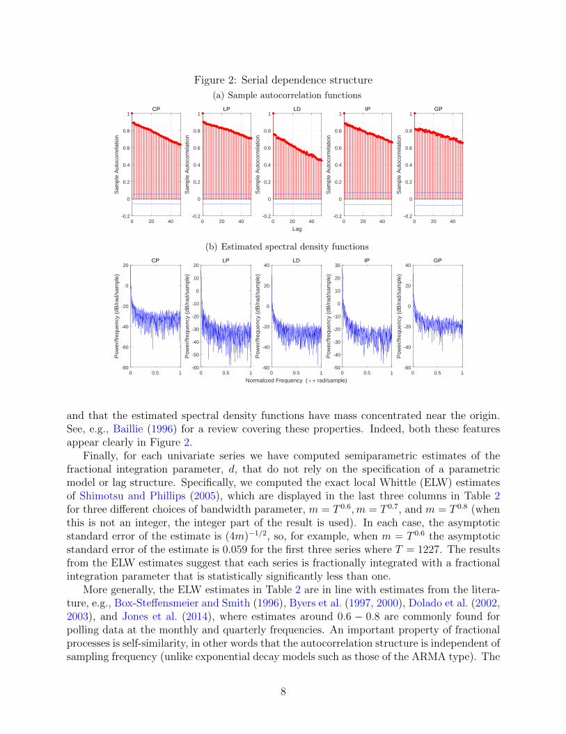
Figure 2: Serial dependence structure

(a) Sample autocorrelation functions

0 20 40-0.2

0

0.2

0.4

0.6

0.8

1S

ampl

e A

utoc

orre

latio

nCP

0 20 40-0.2

0

0.2

0.4

0.6

0.8

1

Sam

ple

Aut

ocor

rela

tion

LP

0 20 40

Lag

-0.2

0

0.2

0.4

0.6

0.8

1

Sam

ple

Aut

ocor

rela

tion

LD

0 20 40-0.2

0

0.2

0.4

0.6

0.8

1

Sam

ple

Aut

ocor

rela

tion

IP

0 20 40-0.2

0

0.2

0.4

0.6

0.8

1

Sam

ple

Aut

ocor

rela

tion

GP

(b) Estimated spectral density functions

0 0.5 1-80

-60

-40

-20

0

20

Pow

er/fr

eque

ncy

(dB

/rad

/sam

ple)

CP

0 0.5 1-60

-50

-40

-30

-20

-10

0

10

20

Pow

er/fr

eque

ncy

(dB

/rad

/sam

ple)

LP

0 0.5 1

Normalized Frequency (×π rad/sample)

-60

-40

-20

0

20

40

Pow

er/fr

eque

ncy

(dB

/rad

/sam

ple)

LD

0 0.5 1-50

-40

-30

-20

-10

0

10

20

30

Pow

er/fr

eque

ncy

(dB

/rad

/sam

ple)

IP

0 0.5 1-60

-40

-20

0

20

40

Pow

er/fr

eque

ncy

(dB

/rad

/sam

ple)

GP

and that the estimated spectral density functions have mass concentrated near the origin.See, e.g., Baillie (1996) for a review covering these properties. Indeed, both these featuresappear clearly in Figure 2.

Finally, for each univariate series we have computed semiparametric estimates of thefractional integration parameter, d, that do not rely on the specification of a parametricmodel or lag structure. Specifically, we computed the exact local Whittle (ELW) estimatesof Shimotsu and Phillips (2005), which are displayed in the last three columns in Table 2for three different choices of bandwidth parameter, m = T 0.6,m = T 0.7, and m = T 0.8 (whenthis is not an integer, the integer part of the result is used). In each case, the asymptoticstandard error of the estimate is (4m)−1/2, so, for example, when m = T 0.6 the asymptoticstandard error of the estimate is 0.059 for the first three series where T = 1227. The resultsfrom the ELW estimates suggest that each series is fractionally integrated with a fractionalintegration parameter that is statistically significantly less than one.

More generally, the ELW estimates in Table 2 are in line with estimates from the litera-ture, e.g., Box-Steffensmeier and Smith (1996), Byers et al. (1997, 2000), Dolado et al. (2002,2003), and Jones et al. (2014), where estimates around 0.6 − 0.8 are commonly found forpolling data at the monthly and quarterly frequencies. An important property of fractionalprocesses is self-similarity, in other words that the autocorrelation structure is independent ofsampling frequency (unlike exponential decay models such as those of the ARMA type). The

8

fact that the fractional parameters estimated here using daily data are generally very closeto estimates obtained using monthly and quarterly data is thus another important reasonfor favouring the fractional approach. The evidence presented here clearly shows fractionalintegration characteristics for political opinion polls at the daily frequency, as suggested byboth the self-similarity property and the theoretical (aggregation-based) arguments discussedearlier.

3 Statistical methodology: FCVAR model

Our analysis applies the FCVAR model of Johansen (2008) and Johansen and Nielsen (2012).This model is a generalization of Johansen’s (1995) CVAR model to allow for fractionallyintegrated and fractionally cointegrated time series.

3.1 Variants of the FCVAR model and interpretations

For a time series Yt of dimension p, the well-known CVAR model with a so-called “restrictedconstant” term is given in error correction form as

∆Yt = α(β′Yt−1 + ρ′) +k∑i=1

Γi∆Yt−i + εt = αL(β′Yt + ρ′) +k∑i=1

ΓiLi∆Yt + εt, (4)

where, as usual, εt is a p-dimensional independent and identically distributed error term withmean zero and covariance matrix Ω. The simplest way to derive the FCVAR model fromthe CVAR model is to replace the difference and lag operators, ∆ and L = 1 − ∆, in (4)by their fractional counterparts, ∆b and Lb = 1 −∆b, respectively, and apply the resultingmodel to Yt = ∆d−bXt. We then obtain3

∆dXt = α∆d−bLb(β′Xt + ρ′) +

k∑i=1

Γi∆dLibXt + εt, (5)

where ∆d is the fractional difference operator, and Lb = 1−∆b is the fractional lag operator.4

Model (5) nests Johansen’s (1995) CVAR model in (4) as the special case d = b = 1.Some of the parameters are well-known from the CVAR model and these have the usualinterpretations also in the FCVAR model. The most important of these are the long-runparameters α and β, which are p× r matrices with 0 ≤ r ≤ p, and ρ, which is an r-vector.The rank r is termed the cointegration, or sometimes cofractional, rank. The columns ofβ constitute the r cointegration (cofractional) vectors, such that β′Xt are the cointegratingcombinations of the variables in the system, i.e. the long-run equilibrium relations. Theparameters in α are the adjustment or loading coefficients which represent the speed ofadjustment towards equilibrium for each of the variables. The restricted constant term ρis interpreted as the mean level of the long-run equilibria β′Xt when these are stationary.The short-run dynamics of the variables are governed by the parameters (Γ1, . . . ,Γk) in theautoregressive augmentation.

3In principle, the restricted constant term should be included as ρ′πt(1), where πt(1) denotes the coefficientin (1). This is mathematically convenient, but makes no difference in terms of the practical implementationbecause the infinite summation in (1) needs to be truncated in practice.

4Both the fractional difference and fractional lag operators are defined in terms of their binomial expansionin the lag operator, L, as in (1). Note that the expansion of Lb has no term in L0 and thus only laggeddisequilibrium errors appear in (5).

9

The FCVAR model has two additional parameters compared with the CVAR model,namely the fractional parameters d and b. Here, d denotes the fractional integration orderof the observable time series, while the parameter b determines the degree of fractionalcointegration, i.e. the reduction in fractional integration order of β′Xt compared to Xt itself.Both fractional parameters are estimated jointly with the other parameters, see Section 3.2.The FCVAR model (5) thus has the same main structure as the standard CVAR model (4),in that it allows for modeling of both cointegration and adjustment towards equilibrium, butis more general since it accommodates fractional integration and cointegration.

We note that the fractional difference as defined in (1) is an infinite series, but anyobserved sample will include only a finite number of observations. This makes calculation ofthe fractional differences as defined in (1) impossible. In practice, therefore, the summationin (1) would need to be truncated at n = t − 1, and the bias introduced by application ofsuch a truncation is analyzed by Johansen and Nielsen (2016) using higher-order expansionsin a simpler model. They show, albeit in a simpler model, that this bias can be avoided byincluding a level parameter, µ, that shifts each of the series by a constant. We follow thissuggestion and also consider the unobserved components formulation

Xt = µ+X0t , ∆dX0

t = α∆d−bLbβ′X0

t +k∑i=1

Γi∆dLibX

0t + εt, (6)

from which we easily derive the model

∆d(Xt − µ) = αβ′∆d−bLb(Xt − µ) +k∑i=1

Γi∆dLib(Xt − µ) + εt. (7)

The formulation (7) includes the restricted constant, which may be obtained as ρ′ = −β′µ.More generally, the level parameter µ in (7) is meant to accommodate a non-zero startingpoint for the first observation on the process, i.e., for X1; see Johansen and Nielsen (2016).

Our forecasting analysis applies the versions of the FCVAR model given in (5) and (7)and we provide comparisons with the CVAR model in (4) as our multivariate benchmarkmodel. Following the work of Jones et al. (2014) we also consider the sub-models obtainedby setting d = b in (5) and (7), which results in disequilibrium errors that are I(0). Thus,the four variants of the FCVAR model that we consider are

1. FCVARd,b,ρ: model (5) with restricted constant ρ and fractional parameters d and b,

2. FCVARd,b,µ: model (7) with level parameter µ and fractional parameters d and b,

3. FCVARd=b,ρ: model (5) with restricted constant ρ and fractional parameter d = b,

4. FCVARd=b,µ: model (7) with level parameter µ and fractional parameter d = b.

In each model the fractional parameters are estimated as described in the next subsection,possibly with the restriction d = b imposed as appropriate.

3.2 Maximum likelihood estimation

The models (5) and (7) are estimated by conditional maximum likelihood. It is assumed thata sample of length T+N is available on Xt, where N denotes the number of observations used

10

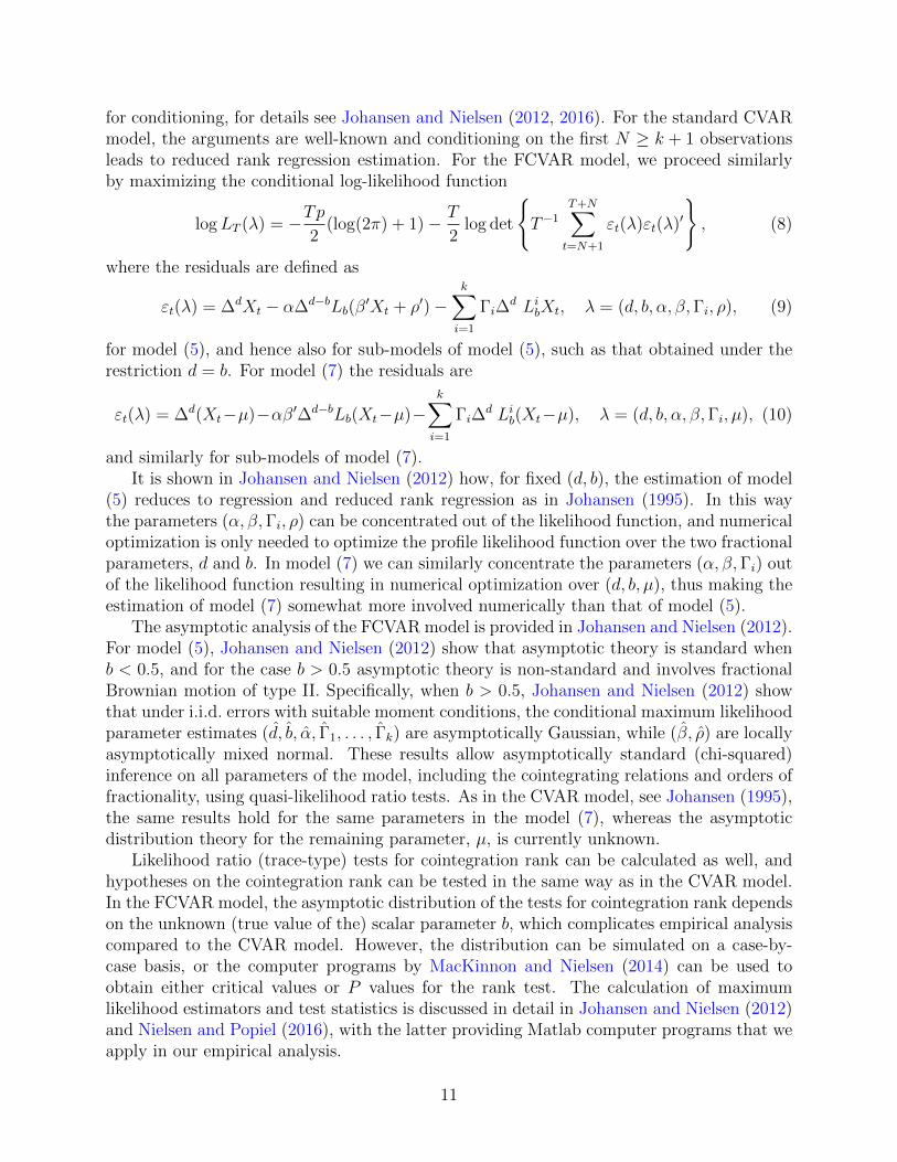
for conditioning, for details see Johansen and Nielsen (2012, 2016). For the standard CVARmodel, the arguments are well-known and conditioning on the first N ≥ k + 1 observationsleads to reduced rank regression estimation. For the FCVAR model, we proceed similarlyby maximizing the conditional log-likelihood function

logLT (λ) = −Tp2

(log(2π) + 1)− T

2log det

T−1

T+N∑t=N+1

εt(λ)εt(λ)′

, (8)

where the residuals are defined as

εt(λ) = ∆dXt − α∆d−bLb(β′Xt + ρ′)−

k∑i=1

Γi∆d LibXt, λ = (d, b, α, β,Γi, ρ), (9)

for model (5), and hence also for sub-models of model (5), such as that obtained under therestriction d = b. For model (7) the residuals are

εt(λ) = ∆d(Xt−µ)−αβ′∆d−bLb(Xt−µ)−k∑i=1

Γi∆d Lib(Xt−µ), λ = (d, b, α, β,Γi, µ), (10)

and similarly for sub-models of model (7).It is shown in Johansen and Nielsen (2012) how, for fixed (d, b), the estimation of model

(5) reduces to regression and reduced rank regression as in Johansen (1995). In this waythe parameters (α, β,Γi, ρ) can be concentrated out of the likelihood function, and numericaloptimization is only needed to optimize the profile likelihood function over the two fractionalparameters, d and b. In model (7) we can similarly concentrate the parameters (α, β,Γi) outof the likelihood function resulting in numerical optimization over (d, b, µ), thus making theestimation of model (7) somewhat more involved numerically than that of model (5).

The asymptotic analysis of the FCVAR model is provided in Johansen and Nielsen (2012).For model (5), Johansen and Nielsen (2012) show that asymptotic theory is standard whenb < 0.5, and for the case b > 0.5 asymptotic theory is non-standard and involves fractionalBrownian motion of type II. Specifically, when b > 0.5, Johansen and Nielsen (2012) showthat under i.i.d. errors with suitable moment conditions, the conditional maximum likelihoodparameter estimates (d, b, α, Γ1, . . . , Γk) are asymptotically Gaussian, while (β, ρ) are locallyasymptotically mixed normal. These results allow asymptotically standard (chi-squared)inference on all parameters of the model, including the cointegrating relations and orders offractionality, using quasi-likelihood ratio tests. As in the CVAR model, see Johansen (1995),the same results hold for the same parameters in the model (7), whereas the asymptoticdistribution theory for the remaining parameter, µ, is currently unknown.

Likelihood ratio (trace-type) tests for cointegration rank can be calculated as well, andhypotheses on the cointegration rank can be tested in the same way as in the CVAR model.In the FCVAR model, the asymptotic distribution of the tests for cointegration rank dependson the unknown (true value of the) scalar parameter b, which complicates empirical analysiscompared to the CVAR model. However, the distribution can be simulated on a case-by-case basis, or the computer programs by MacKinnon and Nielsen (2014) can be used toobtain either critical values or P values for the rank test. The calculation of maximumlikelihood estimators and test statistics is discussed in detail in Johansen and Nielsen (2012)and Nielsen and Popiel (2016), with the latter providing Matlab computer programs that weapply in our empirical analysis.

11

3.3 Forecasting from the FCVAR model

We now discuss how to forecast the (logit transformed) polling data, that is Xt, from theFCVAR model (since the CVAR model is a special case obtained as d = b = 1, forecastsfrom that model are derived in the same way). Because the model is autoregressive, thebest (minimum mean squared error) linear predictor takes a simple form and is relativelystraightforward to calculate. We first note that

∆d(Xt+1 − µ) = Xt+1 − µ− (Xt+1 − µ) + ∆d(Xt+1 − µ) = Xt+1 − µ− Ld(Xt+1 − µ)

and then rearrange (7) as

Xt+1 = µ+ Ld(Xt+1 − µ) + αβ′∆d−bLb(Xt+1 − µ) +k∑i=1

Γi∆dLib(Xt+1 − µ) + εt+1. (11)

Since Lb = 1−∆b is a lag operator, so that LibXt+1 is known at time t for i ≥ 1, this equationcan be used as the basis to calculate forecasts from the model.

We let conditional expectation given the information set at time t be denoted Et(·), andthe best (minimum mean squared error) linear predictor forecast of any variable Zt+1 giveninformation available at time t be denoted Zt+1|t = Et(Zt+1). Clearly, we then have that

the forecast of the innovation for period t + 1 at time t is εt+1|t = Et(εt+1) = 0, and Xt+1|tis then easily found from (11). Inserting coefficient estimates based on data available up totime t, denoted5 (d, b, µ, α, β, Γ1, . . . , Γk), we have that

Xt+1|t = µ+ Ld(Xt+1 − µ) + αβ′∆d−bLb(Xt+1 − µ) +k∑i=1

Γi∆dLi

b(Xt+1 − µ). (12)

This defines the one-step ahead forecast of Xt+1 given information at time t.Multi-period ahead forecasts can be generated recursively. That is, to calculate the h-step

ahead forecast, we first generalize (12) as

Xt+j|t = µ+ Ld(Xt+j|t − µ) + αβ′∆d−bLb(Xt+j|t − µ) +k∑i=1

Γi∆dLi

b(Xt+j|t − µ), (13)

where Xs|t = Xs for s ≤ t. Then forecasts are calculated recursively from (13) for j =

1, 2, . . . , h to generate h-step ahead forecasts, Xt+h|t.Clearly, one-step ahead and h-step ahead forecasts for the model (5) with a restricted

constant term instead of the level parameter can be calculated entirely analogously. We willapply the forecasts (12) and (13) for both models (5) and (7) in our analysis below for severalforecast horizons, h.

4 Forecasting analysis

In this section we present and discuss our main forecasting analysis. In the first subsectionwe briefly discuss some preliminary estimation results to introduce and compare the differentvariants of the FCVAR model, and the next two subsections then present the forecastingprocedure and the corresponding results.

5To emphasize that these estimates are based on data available at time t, they could be denoted by asubscript t. However, to avoid cluttering the notation we omit this subscript and let it be understood in thesequel.

12

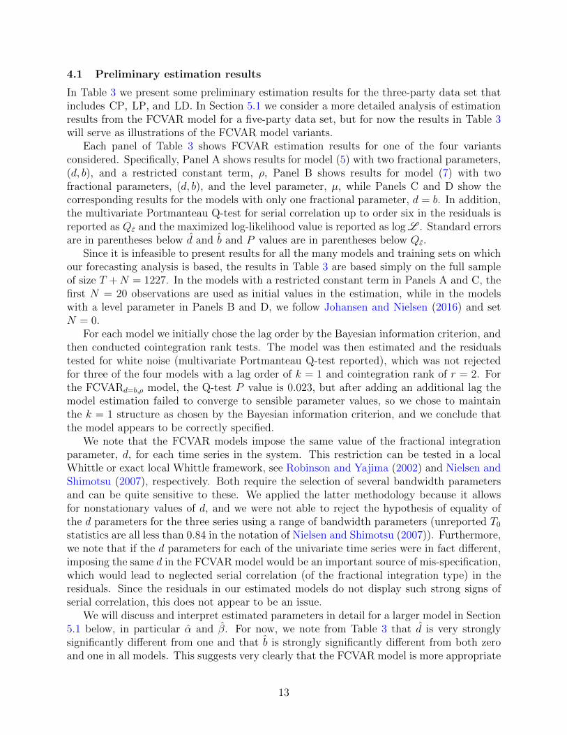
4.1 Preliminary estimation results

In Table 3 we present some preliminary estimation results for the three-party data set thatincludes CP, LP, and LD. In Section 5.1 we consider a more detailed analysis of estimationresults from the FCVAR model for a five-party data set, but for now the results in Table 3will serve as illustrations of the FCVAR model variants.

Each panel of Table 3 shows FCVAR estimation results for one of the four variantsconsidered. Specifically, Panel A shows results for model (5) with two fractional parameters,(d, b), and a restricted constant term, ρ, Panel B shows results for model (7) with twofractional parameters, (d, b), and the level parameter, µ, while Panels C and D show thecorresponding results for the models with only one fractional parameter, d = b. In addition,the multivariate Portmanteau Q-test for serial correlation up to order six in the residuals isreported as Qε and the maximized log-likelihood value is reported as log L . Standard errorsare in parentheses below d and b and P values are in parentheses below Qε.

Since it is infeasible to present results for all the many models and training sets on whichour forecasting analysis is based, the results in Table 3 are based simply on the full sampleof size T +N = 1227. In the models with a restricted constant term in Panels A and C, thefirst N = 20 observations are used as initial values in the estimation, while in the modelswith a level parameter in Panels B and D, we follow Johansen and Nielsen (2016) and setN = 0.

For each model we initially chose the lag order by the Bayesian information criterion, andthen conducted cointegration rank tests. The model was then estimated and the residualstested for white noise (multivariate Portmanteau Q-test reported), which was not rejectedfor three of the four models with a lag order of k = 1 and cointegration rank of r = 2. Forthe FCVARd=b,ρ model, the Q-test P value is 0.023, but after adding an additional lag themodel estimation failed to converge to sensible parameter values, so we chose to maintainthe k = 1 structure as chosen by the Bayesian information criterion, and we conclude thatthe model appears to be correctly specified.

We note that the FCVAR models impose the same value of the fractional integrationparameter, d, for each time series in the system. This restriction can be tested in a localWhittle or exact local Whittle framework, see Robinson and Yajima (2002) and Nielsen andShimotsu (2007), respectively. Both require the selection of several bandwidth parametersand can be quite sensitive to these. We applied the latter methodology because it allowsfor nonstationary values of d, and we were not able to reject the hypothesis of equality ofthe d parameters for the three series using a range of bandwidth parameters (unreported T0statistics are all less than 0.84 in the notation of Nielsen and Shimotsu (2007)). Furthermore,we note that if the d parameters for each of the univariate time series were in fact different,imposing the same d in the FCVAR model would be an important source of mis-specification,which would lead to neglected serial correlation (of the fractional integration type) in theresiduals. Since the residuals in our estimated models do not display such strong signs ofserial correlation, this does not appear to be an issue.

We will discuss and interpret estimated parameters in detail for a larger model in Section5.1 below, in particular α and β. For now, we note from Table 3 that d is very stronglysignificantly different from one and that b is strongly significantly different from both zeroand one in all models. This suggests very clearly that the FCVAR model is more appropriate

13

Table 3: Preliminary estimation results: three parties

Panel A: FCVARd,b,ρ model, k = 1

d = 0.774(0.023)

, b = 0.094(0.026)

, α =

0.532 −0.8100.405 0.0345.517 10.748

, β =

1.000 0.0000.000 1.0002.247 −1.962

,ρ =

[0.019 −1.536

], Γ =

−6.011 0.970 −2.485−0.250 −5.686 −0.684−5.875 −10.224 2.080

,Qε = 50.111

(0.625), log L = 4898.335

Panel B: FCVARd,b,µ model, k = 1

d = 0.624(0.026)

, b = 0.273(0.084)

, α =

0.009 −0.1560.448 0.6470.064 −0.354

, β =

1.000 0.0000.000 1.0000.947 −0.748

,µ =

−0.396−0.660−1.597

, Γ =

−1.278 0.283 −0.033−0.367 −2.105 0.074−0.308 0.478 −1.924

,Qε = 57.148

(0.359), log L = 4965.089

Panel C: FCVARd=b,ρ model, k = 1

d = 0.627(0.013)

, α =

−0.024 −0.024−0.013 0.005−0.100 0.132

, β =

1.000 0.0000.000 1.0000.370 −0.922

,ρ =

[1.955 −1.652

], Γ =

−0.552 0.054 0.0290.049 −0.587 0.0310.049 −0.031 −0.554

,Qε = 76.692

(0.023), log L = 4875.513

Panel D: FCVARd=b,µ model, k = 1

d = 0.572(0.015)

, α =

−0.022 −0.0180.079 0.055−0.058 −0.048

, β =

1.000 0.0000.000 1.0002.403 −3.679

,µ =

−0.411−0.653−1.574

, Γ =

−0.497 0.075 0.027−0.032 −0.652 0.022−0.061 0.119 −0.694

,Qε = 60.163

(0.263), log L = 4962.473

Notes: The table shows estimation results for the four variations of the FCVAR model. The multivariatePortmanteau Q-test for serial correlation up to order six in the residuals is reported as Qε and the maximizedlog-likelihood value is reported as log L . Standard errors are in parentheses below d and b and the P valueis in parenthesis below Qε. The sample size is T +N = 1227, and the first N = 20 (N = 0) observations areused as initial values in the models with a restricted constant term (level parameter).

14

for this data than the non-fractional CVAR model since the latter has d = b = 1 imposed.Comparing across the models, it appears that the estimates of d are fairly close, rangingfrom 0.57 to 0.77, whereas the estimates of b are quite different in the models with d 6= b inPanels A and B of Table 3.

Further comparison across models leads to consideration of the likelihood ratio test statis-tic for the null hypothesis that d = b. That is, for the models with a restricted constantterm (and N = 20), we can test the null of the model in Panel C against the alternative ofthe model in Panel A, and for the models with a level parameter (and N = 0), we can testthe null of the model in Panel D against the alternative of the model in Panel B. In the firstcase, the likelihood ratio test statistic is 45.644, and in the second case, the likelihood ratiotest statistic is 5.232. In both cases, this is asymptotically chi-squared distributed with onedegree of freedom, so the conclusions of these tests differ somewhat and consequently weproceed with the consideration of all four models.

4.2 Forecasting methodology

The four variants of the FCVAR model presented above are evaluated on their forecastingability relative to a group of popular competing models. The CVAR model (4) serves asthe multivariate benchmark model. The main univariate benchmark is the ARFIMA(p, d, q)model,

A(L)∆d(Xt − µ) = B(L)εt, (14)

where A(L) and B(L) are the autoregressive and moving average polynomials, satisfyingstandard regularity conditions. A special case of (14) is the simple ARFIMA(0, d, 0) model,which is also included because it was found by, e.g., Byers et al. (1997) and Dolado et al.(2002), to fit (monthly) UK polling data well. Finally, another special case of (14) is thestandard ARMA(p, q) model, which we include as the classical univariate benchmark. Es-timation of the univariate models is by minimization of the conditional sum-of-squares, seeBox and Jenkins (1970) for ARMA models and Hualde and Robinson (2011) and Nielsen(2015) for ARFIMA models, while forecasting is done using the best (minimum mean squarederror) linear predictor which appears standard for these models.

The forecasting procedure applies the standard rolling window and recursive forecastingschemes to examine forecasting accuracy. The main distinction between the two schemes ishow they select the training sets used for estimating each model to produce forecasts. Therolling window scheme uses a fixed training set length (usually referred to as a window) thatmoves across the data set. The recursive scheme uses an expanding training set length with afixed start date at the beginning of the data set. In order to assess the forecasting capabilityof each model, it is necessary to generate predictions from a sufficiently large number oftraining sets used to estimate each model, and it is preferable that each training set is longenough for reliable estimation and forecasting.

For the rolling window scheme, each statistical model uses training sets with a fixedlength of T + N = 600 observations, approximately half the length of the data set. Forthe recursive scheme, the first training set includes T + N = 600 observations and eachsubsequent training set includes one more observation, until the last training set which hasT +N = 1227− h observations, where h is the forecast horizon. This implies that for bothforecasting schemes, the total number of training sets is 1227−600−h+1 = 628−h, and thefirst training set is the same for both procedures. For the FCVAR models with a restricted

15

constant term we use the first N = 20 observations of each training set as initial values, andfor the FCVAR models with the level parameter we follow Johansen and Nielsen (2016) anduse N = 0 initial values. The CVAR model applies estimation conditional on N = k + 1initial values, such that maximum likelihood estimation reduces to reduced rank regression.

The forecasting programs use all applicable model specification criteria and tests consis-tently across both the multivariate and univariate model types, and all rejection rules forstatistical hypothesis testing are conducted at the five percent level of significance. For allmodels, the model specification is based on the very first training set, and the same speci-fication is then applied to all training sets. That is, we maintain the same lag orders andcointegration ranks for all training sets, but all the parameters of the models are re-estimatedfor each training set before forecasts are calculated.

The multivariate specifications involve first selecting the lag order, k. Lag order selectionis initially based on the Bayesian information criterion (BIC). Given the lag order, cointe-gration rank tests are performed, which determine the number of cointegrating relations, r,for each model. The multivariate model is then estimated using these values of k and r.In the next step, the program performs a multivariate Portmanteau Q-test for white noiseup to order six on the residuals. If the white noise test rejects, then an additional lag isadded and the rank test, estimation, and white noise test are repeated in sequence until theprogram fails to reject white noise for the residuals. The univariate specification differs fromthe multivariate only in that two lag orders, p and q, need to be selected conditional on theunivariate white noise test failing to reject.

Following the completion of the specification algorithm, the forecasting program estimatesthe model for all training sets and uses the estimated model parameters to generate h-stepahead forecasts for each time series. All multivariate and univariate models consideredgenerate forecasts recursively, see Section 3.3. The ARFIMA(0, d, 0) model is included inthe portfolio due to its popularity for political opinion poll data. Its fixed lag orders makeit the only model in the portfolio with lag orders not determined by a decision rule in theforecasting program.

Forecasts are generated for seven out-of-sample horizons, h: 1, 5, 10, 15, 20, 25, and 50steps ahead. As mentioned above, the number of training sets is different for each forecasthorizon, and we denote this number Mh. The models are ranked based on the multivariate(system) root mean squared forecast error,

RMSFEsys =

√√√√ 1

pMh

p∑i=1

Mh∑j=1

(Xi,Tj+h|Tj −Xi,Tj+h

)2, (15)

as well as the univariate root mean squared forecast errors for each series,

RMSFEi =

√√√√ 1

Mh

Mh∑j=1

(Xi,Tj+h|Tj −Xi,Tj+h

)2, (16)

where, in both cases, h denotes the forecast horizon, p = 3 is the number of series, i.e., thedimension of the multivariate system, Mh = 628 − h is the number of training sets, and Tjis the terminal date of training set j. The individual RMSFEi (i = CP, LP, LD) measuresthe typical magnitude of forecast errors for each individual time series, while the RMSFEsys

measures the typical magnitude of all forecast errors produced by each model.

16

4.3 Forecasting results

This section discusses the forecast performance results and concludes with several figures offorecasts generated by all models in the portfolio.

Tables 4 and 5 report the RMSFEi (i = CP, LP, LD) and RMSFEsys values for the rollingand recursive schemes, respectively. Numbers in parentheses are the corresponding rankingsat each individual forecast horizon. The models are ranked based on the RMSFEsys becausefor each model it provides a single measurement of forecast accuracy for all three time series.We note that the ARFIMA(p, d, q) model specifies both lag orders to be zero, i.e. p = q =0, for all three series, so that the results for the ARFIMA(p, d, q) and ARFIMA(0, d, 0)models are identical, and therefore we do not report the ARFIMA(0, d, 0) results. Giventhe results from the literature cited in Section 2 above, this univariate model specificationis not surprising. We also note that the ARMA(p, q) model specifies (p, q) = (0, 1) for allthree series by a very slim margin over (p, q) = (1, 0) in terms of the BIC; the forecastperformance (unreported) with (p, q) = (1, 0) is qualitatively very similar to that reportedwith (p, q) = (0, 1).

We begin the assessment of the forecast accuracy with a discussion of the one-step aheadforecasts. This seems natural prior to examining performance at other subjectively selectedhorizons that may be of interest in any given application. In the context of political opinionpolls, one can easily imagine the relevance of forecasting poll standings or vote shares atmany different horizons.

According to the recursive scheme, all four variants of the FCVAR model outperformall competing models at the one-step ahead forecasting horizon. According to the rollingwindow scheme, three of the four FCVAR variants outperform all competing models, and theFCVARd=b,ρ model is tied with the ARFIMA(p, d, q) model. Both forecasting schemes ranka variant of the FCVAR model with two fractional parameters as the top performing model.The rolling window scheme ranks the FCVARd,b,µ and FCVARd,b,ρ models first (tied), whilethe recursive scheme ranks the FCVARd,b,ρ model first and the FCVARd=b,ρ model second.An important observation is that the third and fourth ranked FCVAR specifications arevery close in performance to the top performing variant, showing that the reliability of one-step ahead forecasts generated by the FCVAR model is robust to the number of fractionalparameters and type of deterministic terms used in the specification, at least for this dataset.

The longer forecast horizons considered, 5, 10, 15, 20, 25 and 50 steps ahead, deliverresults that are in agreement with the findings for the one-step ahead horizon. The modelrankings across all forecast horizons determine that the accuracy of both short, medium andlong term forecasts generated by the FCVAR model is better than the other models in theportfolio. This can be seen from the fact that for 14 of 14 cases (1 to 50 steps ahead in boththe rolling and the recursive schemes), the top two performing models are always variants ofthe FCVAR model and three of the top four models are always variants of the FCVAR model.Furthermore, with the exception of one forecast horizon (50 steps ahead) in both schemes,all four variants of the FCVAR model are ranked as the top four models. The exceptionoccurs when only one variant of the FCVAR model underperforms by a small margin relativeto the ARFIMA model. Overall, this evidence provides strong support for the applicationof the FCVAR model for forecasting next day (one-step), next week (5-steps), and all the

17

Table 4: Root mean squared forecast errors – rolling window forecast scheme

Model Series 1 step 5 step 10 step 15 step 20 step 25 step 50 step

FCVARd,b,ρ CP 0.0562 0.0613 0.0637 0.0656 0.0678 0.0704 0.0781LP 0.0499 0.0524 0.0569 0.0609 0.0647 0.0690 0.0902LD 0.1134 0.1161 0.1233 0.1298 0.1358 0.1415 0.1650System 0.0785 (1) 0.0816 (2) 0.0866 (2) 0.0910 (2) 0.0953 (2) 0.0996 (2) 0.1176 (2)

FCVARd,b,µ CP 0.0561 0.0608 0.0632 0.0656 0.0677 0.0702 0.0781LP 0.0505 0.0549 0.0607 0.0669 0.0723 0.0781 0.1030LD 0.1130 0.1145 0.1201 0.1249 0.1295 0.1350 0.1543System 0.0785 (1) 0.0813 (1) 0.0858 (1) 0.0901 (1) 0.0941 (1) 0.0987 (1) 0.1162 (1)

FCVARd=b,ρ CP 0.0569 0.0629 0.0664 0.0684 0.0708 0.0729 0.0782LP 0.0506 0.0525 0.0569 0.0604 0.0645 0.0687 0.0908LD 0.1174 0.1241 0.1329 0.1400 0.1445 0.1499 0.1663System 0.0808 (4) 0.0859 (4) 0.0918 (4) 0.0965 (4) 0.1001 (3) 0.1041 (3) 0.1183 (3)

FCVARd=b,µ CP 0.0566 0.0634 0.0682 0.0731 0.0783 0.0828 0.1039LP 0.0502 0.0540 0.0597 0.0653 0.0705 0.0828 0.1056LD 0.1131 0.1169 0.1242 0.1326 0.1379 0.1450 0.1799System 0.0786 (3) 0.0829 (3) 0.0888 (3) 0.0952 (3) 0.1002 (4) 0.1076 (4) 0.1345 (5)

CVARρ CP 0.0605 0.0656 0.0712 0.0748 0.0800 0.0835 0.0953LP 0.0547 0.0577 0.0667 0.0744 0.0805 0.0865 0.1114LD 0.1200 0.1260 0.1386 0.1489 0.1559 0.1619 0.1828System 0.0838 (6) 0.0885 (6) 0.0979 (6) 0.1054 (6) 0.1113 (6) 0.1164 (6) 0.1353 (6)

ARFIMA(p, d, q) CP 0.0578 0.0623 0.0664 0.0700 0.0730 0.0758 0.0860LP 0.0531 0.0638 0.0746 0.0834 0.0909 0.0977 0.1252LD 0.1158 0.1244 0.1335 0.1410 0.1466 0.1521 0.1707System 0.0808 (4) 0.0884 (5) 0.0963 (5) 0.1029 (5) 0.1081 (5) 0.1132 (5) 0.1319 (4)

ARMA(p, q) CP 0.0899 0.1167 0.1178 0.1187 0.1187 0.1190 0.1207LP 0.1109 0.1582 0.1605 0.1628 0.1650 0.1673 0.1781LD 0.1627 0.1947 0.1957 0.1971 0.1983 0.1997 0.2049System 0.1250 (7) 0.1597 (7) 0.1612 (7) 0.1627 (7) 0.1640 (7) 0.1653 (7) 0.1715 (7)

Notes: The overall performance of each model is measured by the root mean square forecast error of theentire multivariate system. The ARFIMA(0, d, 0) model is not included because the ARFIMA(p, d, q) modelspecifies both lag orders to zero for all three series. The ARMA(p, q) model specifies (p, q) = (0, 1) for allthree series. Numbers in parentheses are the corresponding rankings at each individual forecast horizon.The number 1 rank is assigned to the best performing model and the number 7 rank is assigned to the worstperforming model. Results are based on h-step ahead forecasts produced using 628-h training sets of length600.

way up to ten weeks ahead (50-steps) poll standings.The results for both forecasting schemes suggest that the FCVAR model with two frac-

tional parameters produces the smallest average forecast errors. A variant of the FCVARmodel with two fractional parameters always outperforms both sub-models, the FCVARd=b,ρ

and FCVARd=b,µ, although only by very small margins. The recursive scheme determines theFCVARd,b,ρ model as the absolute favorite at all forecast horizons, while the rolling windowscheme ranks the FCVARd,b,µ model as the favorite at all forecast horizons greater than one-step, and ranks the FCVARd,b,µ and FCVARd,b,ρ models as the top two performing modelsfor next day forecasting.

18

Table 5: Root mean squared forecast errors – recursive window forecast scheme

Model Series 1 step 5 step 10 step 15 step 20 step 25 step 50 step

FCVARd,b,ρ CP 0.0561 0.0616 0.0642 0.0667 0.0697 0.0727 0.0839LP 0.0505 0.0548 0.0611 0.0671 0.0726 0.0784 0.1062LD 0.1123 0.1144 0.1197 0.1251 0.1292 0.1342 0.1520System 0.0781 (1) 0.0814 (1) 0.0860 (1) 0.0906 (1) 0.0946 (1) 0.0991 (1) 0.1175 (1)

FCVARd,b,µ CP 0.0563 0.0619 0.0653 0.0688 0.0728 0.0765 0.0905LP 0.0499 0.0524 0.0564 0.0602 0.0640 0.0686 0.0939LD 0.1150 0.1198 0.1288 0.1381 0.1466 0.1567 0.2024System 0.0793 (3) 0.0835 (3) 0.0895 (4) 0.0956 (4) 0.1015 (4) 0.1082 (4) 0.1390 (5)

FCVARd=b,ρ CP 0.0563 0.0617 0.0646 0.0672 0.0701 0.0732 0.0846LP 0.0507 0.0550 0.0612 0.0673 0.0729 0.0786 0.1058LD 0.1144 0.1193 0.1267 0.1338 0.1387 0.1439 0.1614System 0.0792 (2) 0.0838 (4) 0.0894 (3) 0.0948 (3) 0.0991 (2) 0.1037 (2) 0.1217 (2)

FCVARd=b,µ CP 0.0563 0.0624 0.0662 0.0697 0.0731 0.0766 0.0887LP 0.0507 0.0555 0.0622 0.0685 0.0747 0.0808 0.1113LD 0.1147 0.1171 0.1236 0.1309 0.1367 0.1441 0.1741System 0.0794 (4) 0.0830 (2) 0.0886 (2) 0.0943 (2) 0.0993 (3) 0.1051 (3) 0.1298 (3)

CVARρ CP 0.0615 0.0684 0.0712 0.0830 0.0909 0.0972 0.1160LP 0.0551 0.0595 0.0667 0.0828 0.0926 0.1017 0.1388LD 0.1208 0.1222 0.1386 0.1427 0.1500 0.1572 0.1789System 0.0845 (6) 0.0878 (6) 0.0979 (6) 0.1066 (6) 0.1145 (6) 0.1218 (6) 0.1469 (6)

ARFIMA(p, d, q) CP 0.0585 0.0627 0.0668 0.0706 0.0739 0.0770 0.0881LP 0.0517 0.0566 0.0634 0.0692 0.0744 0.0792 0.0991LD 0.1182 0.1241 0.1359 0.1468 0.1560 0.1651 0.2007System 0.0818 (5) 0.0867 (5) 0.0948 (5) 0.1022 (5) 0.1085 (5) 0.1147 (5) 0.1389 (4)

ARMA(p, q) CP 0.1105 0.1503 0.1511 0.1516 0.1515 0.1517 0.1523LP 0.1157 0.1693 0.1706 0.1719 0.1731 0.1744 0.1808LD 0.1714 0.2124 0.2135 0.2150 0.2165 0.2180 0.2249System 0.1354 (7) 0.1792 (7) 0.1803 (7) 0.1815 (7) 0.1824 (7) 0.1834 (7) 0.1884 (7)

Notes: The overall performance of each model is measured by the root mean square forecast error of theentire multivariate system. The ARFIMA(0, d, 0) model is not included because the ARFIMA(p, d, q) modelspecifies both lag orders to zero for all three series. The ARMA(p, q) model specifies (p, q) = (0, 1) for allthree series. Numbers in parentheses are the corresponding rankings at each individual forecast horizon.The number 1 rank is assigned to the best performing model and the number 7 rank is assigned to theworst performing model. Results are based on h-step ahead forecasts produced using 628-h training sets oflength= 600, 601, . . . , 1227− h.

Thus, the model rankings strongly suggest that the forecasting accuracy of the FCVARis better than both the fractional benchmark model (ARFIMA) and the multivariate bench-mark model (CVAR). To assess the degree of relative performance, Table 6 reports theRMSFE percentage change,

100

(RMSFEsys(FCVAR)

RMSFEsys(ARFIMA)− 1

), (17)

of the FCVAR model relative to the ARFIMA model for the rolling and recursive schemes inPanels A and B, respectively. Negative values favor the FCVAR model and positive values

19

Table 6: Percentage change in RMSFEsys: FCVAR vs. ARFIMA(p, d, q)

Model 1 step 5 step 10 step 15 step 20 step 25 step 50 step

Panel A: rolling scheme

FCVARd,b,ρ −2.79 −7.68 −10.07 −11.53 −11.88 −12.05 −10.87FCVARd,b,µ −2.90 −8.05 −10.87 −12.39 −12.92 −12.77 −11.89FCVARd=b,ρ −0.01 −2.88 −4.62 −6.24 −7.41 −8.05 −10.28FCVARd=b,µ −2.77 −6.26 −7.82 −7.48 −7.31 −4.94 2.01

Panel B: recursive scheme

FCVARd,b,ρ −4.50 −6.10 −9.29 −11.39 −12.85 −13.63 −15.40FCVARd,b,µ −3.01 −3.66 −5.58 −6.44 −6.48 −5.68 0.08FCVARd=b,ρ −3.15 −3.35 −5.71 −7.26 −8.66 −9.61 −12.41FCVARd=b,µ −2.98 −4.22 −6.58 −7.72 −8.43 −8.34 −6.53

Notes: Negative values favor the FCVAR model. Results are based on h-step ahead forecasts produced using628-h training sets of length 600 (rolling scheme) or length= 600, 601, . . . , 1227− h (recursive scheme).

Table 7: Percentage change in RMSFEsys: FCVAR vs. CVAR

Model 1 step 5 step 10 step 15 step 20 step 25 step 50 step

Panel A: rolling scheme

FCVARd,b,ρ −6.24 −7.80 −11.50 −13.60 −14.43 −14.48 −13.10FCVARd,b,µ −6.34 −8.18 −12.29 −14.44 −15.45 −15.19 −14.10FCVARd=b,ρ −3.56 −3.01 −6.14 −8.42 −10.10 −10.60 −12.52FCVARd=b,µ −6.22 −6.39 −9.29 −9.64 −10.00 −7.58 −0.55

Panel B: recursive scheme

FCVARd,b,ρ −7.53 −7.32 −12.13 −15.07 −17.43 −18.66 −20.00FCVARd,b,µ −6.08 −4.92 −8.53 −10.32 −11.39 −11.17 −5.36FCVARd=b,ρ −6.23 −4.61 −8.65 −11.11 −13.45 −14.88 −17.18FCVARd=b,µ −6.06 −5.47 −9.50 −11.55 −13.24 −13.68 −11.61

Notes: Negative values favor the FCVAR model. Results are based on h-step ahead forecasts produced using628-h training sets of length 600 (rolling scheme) or length= 600, 601, . . . , 1227− h (recursive scheme).

favor the ARFIMA model.Previous literature, as cited earlier, has extensively documented the superiority of frac-

tional (ARFIMA) models for modeling and forecasting polling data. Compared to thisimportant benchmark, Table 6 shows that the RMSFE of the FCVAR model is as much as13% lower for the rolling scheme and 15% lower for the recursive scheme. In 54 of 56 cases inTable 6, the multivariate fractional model outperforms the univariate fractional model andin 16 of 56 cases, the FCVAR model delivers more than a 10% reduction in the RMSFEsys

relative to the ARFIMA model. The gains at the longer horizons are more pronounced, andthe gains appear to be larger for the FCVAR models with two fractional parameters.

Similarly, Table 7 reports the RMSFE percentage change of the FCVAR model relative

20

to the CVAR model. Again, this table shows improved forecast accuracy for all variantsof the FCVAR model relative the to the CVAR model. In 56 of 56 cases in Table 7, allfour variants of the FCVAR model perform better than the CVAR model. For the FCVARmodels with a restricted constant, the improvements in performance increase substantiallyas the forecasting horizon increases. The recursive scheme shows 15%, 17%, 19% and 20%improvement for the 15, 20, 25 and 50 step ahead horizons, attained by the FCVAR modelwith two fractional parameters and a restricted constant. The rolling scheme shows upto 14% improvement for the FCVAR models with a restricted constant, and up to 15%improvement for the FCVAR models with a level parameter. In 30 of 56 cases, the FCVARmodel delivers more than a 10% reduction in the RMSFEsys relative to the CVAR model.Overall the fractional models clearly outperform the non-fractional models, with the gainsbecoming more pronounced at longer forecast horizons.

To conclude the forecast comparison, examples of forecasts generated by all models inthe portfolio are presented in Figure 3. The presented forecasts are generated using thefirst training set, which is common to both the rolling and recursive forecasting schemes.The figure shows the last 9 observations in the training set, followed by the out-of-sampleobservations and forecasts beginning at the 10th observation and continuing up to the longesthorizon considered, h = 50, for the CP, LP and LD series in separate graphs. Panel (a)shows forecasts of the logit transformed series, while in Panel (b) all series (and forecasts)are transformed back to percentage vote shares to make interpretations easier. The figurethus provides an illustration of how all models forecast political support as measured bydaily opinion polls. In Panel (a) we also include 90% confidence bands shown using slightlythinner lines.6

The forecasts for this particular training set are in agreement with the evidence presentedin the model ranking exercise. An interesting observation, which is present in results fromother training sets as well, is that even though the CVAR forecasts exhibit more dynamicsin the short run (which is a result of a higher lag order selected compared to the FCVAR),this does not translate into more accurate predictions for short horizons. In particular, asthe short run dynamics die out for all multivariate models, it is evident that fractional coin-tegration generates point forecasts that are closer to the subsequently realized observations.These conclusions are strongly supported by the reported confidence bands in Figure 3(a),which show that forecasts based on the FCVAR models are much more accurate than thosebased on the non-fractional CVAR model. This is especially true at the longer horizons, asone might have expected. Finally, we note that all variants of the FCVAR produce similarpredictions, and these are reasonably close to the realized data series in all three panels,while the other models in the portfolio only perform well in some cases.

5 Empirical application to the 2015 UK general election

In this section we present an application to the 2015 UK general election, which was deemedthe most unpredictable election in decades in the media. Opinion poll agencies predicteda hung parliament, but ended up significantly underestimating the Conservative Party voteshare; the party that won the election with a majority representation in Parliament. Note,

6Following the advice of a referee, these were simply calculated from the moving-average representationof the models ignoring estimation uncertainty.

21

Figure 3: Forecasts for the first training set

(a) Forecasts of logit transformed series

2012-11-05 2013-01-2430

32

34

36

38CP

FCVARd=b,ρ FCVARd=b,µ FCVARd,b,ρ FCVARd,b,µ

2012-11-05 2013-01-2436

38

40

42

44

46LP

Data Mean

2012-11-05 2013-01-247

8

9

10

11

12LD

CVARρ ARFIMA(p, d, q) ARMA(p, q)

2012-11-05 2013-01-24-0.9

-0.8

-0.7

-0.6

-0.5CP

2012-11-05 2013-01-24-0.5

-0.4

-0.3

-0.2

-0.1LP

2012-11-05 2013-01-24-2.8

-2.6

-2.4

-2.2

-2

-1.8LD

2012-11-05 2013-01-24-1

-0.8

-0.6

-0.4

-0.2CP

2012-11-05 2013-01-24-0.8

-0.6

-0.4

-0.2

0LP

2012-11-05 2013-01-24-2.8

-2.6

-2.4

-2.2

-2

-1.8LD

(b) Forecasts of vote shares in percentage

2012-11-05 2013-01-2430

32

34

36

38CP

FCVARd=b,ρ FCVARd=b,µ FCVARd,b,ρ FCVARd,b,µ

2012-11-05 2013-01-2436

38

40

42

44

46LP

Data Mean

2012-11-05 2013-01-247

8

9

10

11

12LD

CVARρ ARFIMA(p, d, q) ARMA(p, q)

2012-11-05 2013-01-24-0.9

-0.8

-0.7

-0.6

-0.5CP

2012-11-05 2013-01-24-0.5

-0.4

-0.3

-0.2

-0.1LP

2012-11-05 2013-01-24-2.8

-2.6

-2.4

-2.2

-2

-1.8LD

2012-11-05 2013-01-24-1

-0.8

-0.6

-0.4

-0.2CP

2012-11-05 2013-01-24-0.8

-0.6

-0.4

-0.2

0LP

2012-11-05 2013-01-24-2.8

-2.6

-2.4

-2.2

-2

-1.8LD

Notes: The training set is the first window, which is shared by the rolling window and recursive windowforecasting schemes. Panel (a) shows forecasts of logit transformed series, where 90% confidence bands areshown using with slightly thinner lines, and Panel (b) shows forecasts of vote shares in percentage. TheARFIMA(0, d, 0) model is not included because the ARFIMA(p, d, q) model specifies both lag orders to zerofor all three series. The ARMA(p, q) model specifies (p, q) = (0, 1) for all three series.

however, that vote shares cannot be mapped into election outcomes in the context of theUK election process. This can be seen from the fact that the realized vote share for theConservative Party was 36.8%, but the party won 330 out of 650 constituencies in thecountry; an outcome that the predicted vote share of the previous-day YouGov opinion poll,34%, does not exclude.

The three political parties represented in the full data set, spanning the entire durationof the survey, are the three major political parties in the UK that have historically hadthe most representation in government by a strong margin over other parties running in

22

Table 8: FCVARd=b,ρ estimation results: five parties

Model:

∆d

CPt

LPt

LDt

IPt

GPt

= α

(β′∆d−bLb

CPt

LPt

LDt

IPt

GPt

+ ρ′

)+ Γ1∆

dLb

CPt

LPt

LDt

IPt

GPt

+ Γ2∆dL2

b

CPt

LPt

LDt

IPt

GPt

+ εt

Parameters:

α =

−0.147 0.140 0.063 0.046

0.019 −0.232 0.070 −0.069−0.038 0.145 −0.425 0.071−0.012 −0.300 0.018 −0.083−0.872 −1.549 −0.752 −0.335

, β =

1.000 0.000 0.000 0.0000.000 1.000 0.000 0.0000.000 0.000 1.000 0.0000.000 0.000 0.000 1.0000.170 −0.604 0.510 2.760

d = 0.813

(0.016), ρ =

[1.068 −0.555 3.872 7.821

]Qε = 166.098

(0.175), log L = 3632.605

Notes: The table shows FCVAR estimation results for model (5) with one fractional parameter, d = b, anda restricted constant term, ρ. The multivariate Portmanteau Q-test for serial correlation up to order six inthe residuals is reported as Qε and the maximized log-likelihood value is reported as log L . The standarderror is in parenthesis below d and the P value is in parenthesis below Qε. The sample size is T +N = 729and the first N = 20 observations are used as initial values.

the election. However, as the 2015 general election has shown, other parties not in the topthree (as measured by representation in parliament or by opinion polls) can be importantplayers. In this election, the UKIP and the Green Party received 12.7% and 3.8% vote shares,in particular. As discussed earlier, on April 16th, 2012, and June 18th, 2012, respectively,YouGov changed the way they reported the outcomes of their polls and started reportingthe UKIP and the Green Party as separate time series (rather than being included in theresidual category). Therefore, in this empirical application to the 2015 UK general election,we apply the multivariate and univariate models to both the case of three political parties(based on the full sample spanning the entire 2010 to 2015 political cycle) and to the caseof either four or five political parties (based on shorter data sets spanning only the secondhalf of the 2010 to 2015 political cycle).7

A key strength of our data set for the purpose of statistical modeling and forecasting,and hence for vote share prediction, is that the observed time series are contained withinone political cycle. This should allow application of a relatively simple statistical model, andthe previous analysis has shown strong support for the FCVAR model for this task.

23

5.1 Estimation results prior to the election

In the first part of this empirical application, we analyze and interpret the estimated modelcoefficients more carefully. To this end, we consider the full five-party data set consisting ofCPt, LPt, LDt, IPt, and GPt, but for a reduced sample size covering June 18th, 2012, to May6th, 2015, for a total of T +N = 729 observations, which is the period where observations areavailable for all five parties. The increased dimension of the model tends to cause problemsin the multi-dimensional numerical optimization required for the FCVAR models with eithertwo fractional parameters or with the level parameter, and for this reason we consider onlythe FCVARd=b,ρ model for the full data set, since this model requires only one-dimensionalnumerical optimization and thus remains feasible.

As usual, the estimation begins with lag length selection. The BIC first suggests k = 1,but for this choice the Portmanteau Q-test rejects the null of no serial correlation in theresiduals with a P value of 0.000. Consequently, we increase the lag length to k = 2 forwhich the Q-test P value is 0.17. Next, the LR test for cointegration rank (the trace test)produces P values of 0.051 and 0.977 for r = 3 and r = 4, respectively, and we proceed withthe specification r = 4. As before, all results are conditional upon N = 20 initial values.

The estimation results for the FCVARd=b,ρ model for the five-party data set are presentedin Table 8. We focus our interpretations on the long-run cointegration parameters, α and β.

To interpret the estimated cointegrating relations in β, we find it convenient to re-normalize them on the coefficient for the Conservatives. That is, we re-normalize β suchthat

β =

−1 −1 −1 −1βLP 0 0 0

0 βLD 0 00 0 β IP 00 0 0 βGP

. (18)

We note that this is simply a re-normalization because a similar rotation of the α matriximplies that the product αβ′, and hence the likelihood, is unchanged. The normalization in(18) implies that each cointegrating relation takes the form

CPt = βSSt for S ∈ LP, LD, IP, GP.

Thus, the normalization of β given in (18) seems more straightforward to interpret becauseit directly relates the vote shares of each party to that of a main party, CP, rather than thatof GP.

Applying the normalization in (18) to β in Table 8, we find

βLP = −0.282, βLD = 0.334, β IP = 0.062, βGP = −0.170.

It it now clear that the government parties, CP and LD, move together in the long-run,although movements in the LD poll share are only about 1/3 of those in the CP poll share.It also seems that the IP poll share moves in the same direction as CP, but again with acoefficient less than one. On the other hand, the poll shares of both opposition parties, LPand GP, move in the opposite direction of the government parties, as expected.

7There were also some regional parties with non-negligible vote shares, but we do not include these inour analysis because they seem to compete on a different basis and with a somewhat different agenda.

24

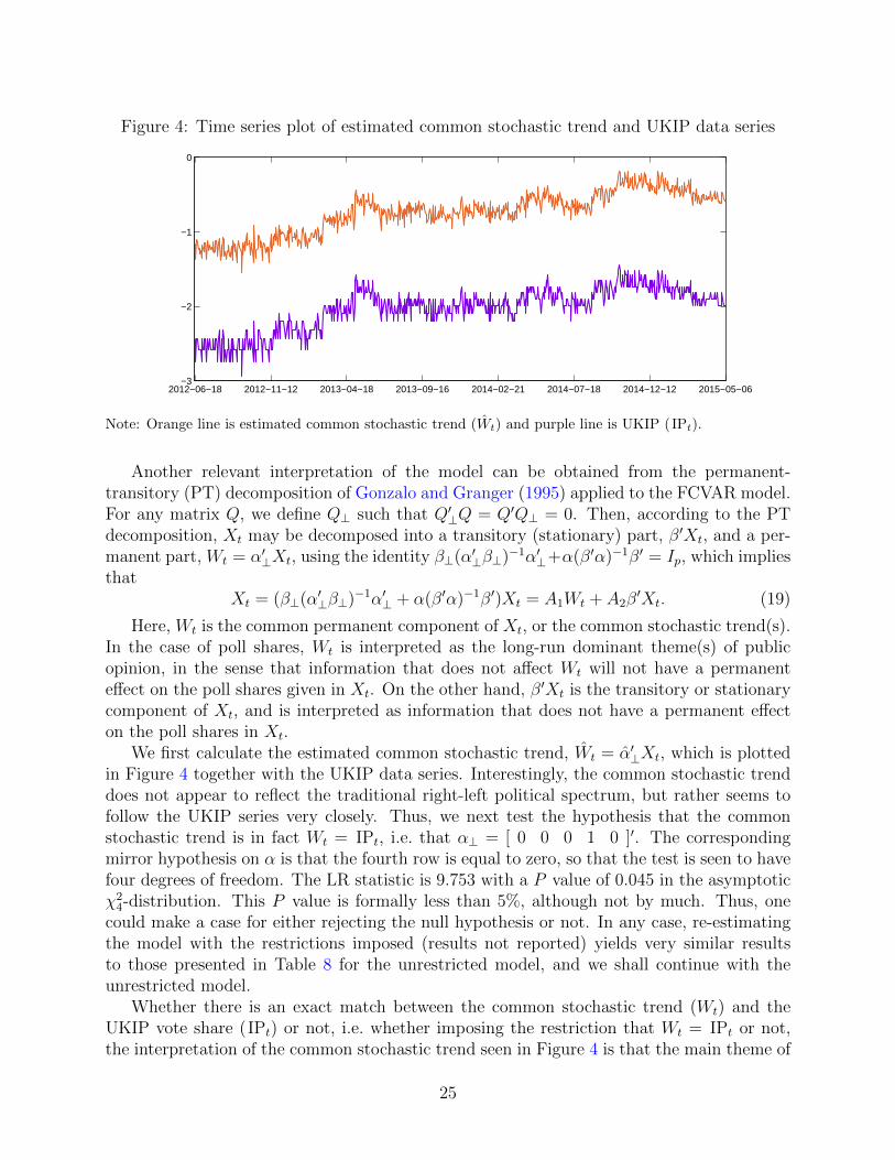
Figure 4: Time series plot of estimated common stochastic trend and UKIP data series

2012−06−18 2012−11−12 2013−04−18 2013−09−16 2014−02−21 2014−07−18 2014−12−12 2015−05−06−3

−2

−1

0

Note: Orange line is estimated common stochastic trend (Wt) and purple line is UKIP (IPt).

Another relevant interpretation of the model can be obtained from the permanent-transitory (PT) decomposition of Gonzalo and Granger (1995) applied to the FCVAR model.For any matrix Q, we define Q⊥ such that Q′⊥Q = Q′Q⊥ = 0. Then, according to the PTdecomposition, Xt may be decomposed into a transitory (stationary) part, β′Xt, and a per-manent part, Wt = α′⊥Xt, using the identity β⊥(α′⊥β⊥)−1α′⊥+α(β′α)−1β′ = Ip, which impliesthat

Xt = (β⊥(α′⊥β⊥)−1α′⊥ + α(β′α)−1β′)Xt = A1Wt + A2β′Xt. (19)

Here, Wt is the common permanent component of Xt, or the common stochastic trend(s).In the case of poll shares, Wt is interpreted as the long-run dominant theme(s) of publicopinion, in the sense that information that does not affect Wt will not have a permanenteffect on the poll shares given in Xt. On the other hand, β′Xt is the transitory or stationarycomponent of Xt, and is interpreted as information that does not have a permanent effecton the poll shares in Xt.

We first calculate the estimated common stochastic trend, Wt = α′⊥Xt, which is plottedin Figure 4 together with the UKIP data series. Interestingly, the common stochastic trenddoes not appear to reflect the traditional right-left political spectrum, but rather seems tofollow the UKIP series very closely. Thus, we next test the hypothesis that the commonstochastic trend is in fact Wt = IPt, i.e. that α⊥ = [ 0 0 0 1 0 ]′. The correspondingmirror hypothesis on α is that the fourth row is equal to zero, so that the test is seen to havefour degrees of freedom. The LR statistic is 9.753 with a P value of 0.045 in the asymptoticχ24-distribution. This P value is formally less than 5%, although not by much. Thus, one

could make a case for either rejecting the null hypothesis or not. In any case, re-estimatingthe model with the restrictions imposed (results not reported) yields very similar resultsto those presented in Table 8 for the unrestricted model, and we shall continue with theunrestricted model.

Whether there is an exact match between the common stochastic trend (Wt) and theUKIP vote share (IPt) or not, i.e. whether imposing the restriction that Wt = IPt or not,the interpretation of the common stochastic trend seen in Figure 4 is that the main theme of

25

political debate in the UK during this time period from June 18th, 2012, to May 6th, 2015,has revolved around the independence question in relation to the European Union, at leastin terms of long-run movements of poll shares. We proceed to calculate the coefficient onWt in (19), which yields

A1 = [ 0.076 −0.269 0.228 1.230 −0.446 ]′

for the unrestricted model (i.e., without imposing Wt = IPt). For the restricted model(imposing Wt = IPt), the results are qualitatively similar.

Interpreting Wt as a measure of the strength of Euro-skepticism in public opinion, theestimated coefficients in A1 suggest that, as Euro-skepticism gains ground and Wt increases,this leads to a large increase in popularity of the UKIP. However, when Wt increases, thegovernment parties (CP and LD) also increase in popularity, whereas the opposition parties(LP and GP) decrease in popularity.8

5.2 Predicting vote shares of the election

The UKIP and Green Party poll series exhibit an important caveat, which is that unlikethe three major political parties, the UKIP and the Green Party are not stated explicitlyas choices in the survey question posed to the poll participants. In the forecasting analysiswe do not include the Green Party because doing so would further reduce the sample sizeand the increased dimension of the model tends to cause problems in the multi-dimensionalnumerical optimization required for the FCVAR models with either two fractional parametersor with the level parameter. Thus, in the forecasting analysis we consider either three parties(CPt, LPt, and LDt) or four parties (including also IPt).

We next present predictions of all models in the portfolio leading into the 56th UK generalelection held on May 7th, 2015. Specifically, Tables 9 (three parties) and 10 (four parties)show the opinion poll and the election vote share predictions of each model one month,one week and one day preceding the election day, as well as the final election vote shareoutcome. The predicted values represent forecasts of the poll standings which can be viewedas predicted vote shares for each political party.

Relative to the poll predictions on May 6th, 2015, which underestimated the vote shareof the Conservative Party and overestimated the vote shares for Labour and the LiberalDemocrats, the forecasts in both Table 9 and Table 10 show that all models in the portfoliopredicted a fall in the vote share for the Liberal Democrats, in agreement with the realizedvote share. The three-party forecasts in Table 9 generated on the day before the election(Panel C) show that (i) all models predicted vote shares very similar to the poll predictionsfor the Conservative Party and the Labour Party (with the exception of the ARMA predictionfor the Labour Party), (ii) the two FCVAR models with a level parameter and the CVARmodel predicted vote shares closest to the election outcomes for the Labour Party, and (iii)the multivariate models predicted vote shares closest to the election outcomes for the LiberalDemocrats. The four-party forecasts in Table 10 generated on the day before the election(Panel C) show that (i) variants of the FCVAR model predicted vote shares that are closestto the election outcome for the Conservative Party, (ii) with the exception of the ARMA

8Recall that the poll shares are logit transformed. Because of this nonlinear transformation, absolutemagnitudes of the coefficients are difficult to interpret, and, in particular, there is no requirement that thecoefficients sum to zero.

26

model all models show similar predictions for the Labour Party, (iii) the multivariate modelspredicted vote shares closest to the election outcomes for the Liberal Democrats, and (iv)with the exception of the CVAR model all models show similar predictions for the UKIP.

As shown in Tables 9 and 10, the opinion polls severely underestimated the ConservativeParty vote shares in the election and similarly overestimated the Labour Party vote shares.Since all statistical models considered here rely solely on the opinion poll series for infor-mation, it is not surprising that for political parties for which the election result stronglydeviated from the opinion poll prediction, the statistical models find it difficult to predictthe high realized vote shares for the Conservative Party and low realized vote shares for theLabour Party. It is in this context that the evolution of the predictions serves to comple-ment opinion polls, since as the most recent poll data became available, forecasters wouldnaturally obtain forecasts for the election.

To illustrate how the analysis presented in this paper complements the industry standardof using the latest opinion poll as an indicator of future political support, we examine theevolution of the model predictions as the observed data approaches the election day on May7th, 2015, which allows the analyst to monitor the dynamics of the opinion poll and themodel predictions. Figures 5 and 6 show forecasts by all models over 50 polling days leadinginto the election, for the three-party and the four-party analysis, respectively. That is, attime h polling days prior to the election, each figure shows the h-step ahead predictions fromeach model. Panel (a) of each figure shows forecasts of the logit transformed series, where90% confidence bands are shown using slightly thinner lines, and Panel (b) of each figureshows forecasts of vote shares in percentage. With these plots, we can analyze the dynamicsof model forecasts leading into a particular date of interest, in this case the election day, andcompare both across models and with the actual daily poll series.

For the three-party analysis in Figure 5, the evolution of forecasts for all FCVAR modelvariants show an upward trend in the support for the Conservative Party leading into theelection, and a downward trend for the Labour Party for one week leading into the election.These two trends project the correct direction for the realized vote shares in the election.For the Liberal Democrats, the strong upward trends in the predicted vote share, as shownby nearly all models, tend to follow the opinion poll and is therefore suspect to exhibit thesame tendency as political polls, in that they tend to over-represent support for smallerpolitical parties when compared to the election vote share outcomes and the representationin government.

For all models, the confidence bands in Figure 5(a) become narrower as the electionapproaches, which is expected because the forecast horizon shortens. For all the multivariatemodels, the election outcomes for both the Conservative Party and the Labour Party lieoutside the confidence bands for most of the time period considered in the figure. For theunivariate models, the confidence bands are wider and include the Conservative Party andLabour Party election outcomes for a large part of the sampling period (except the ARMAmodel for LP). For the Liberal Democrats the confidence bands of all models include theelection outcome throughout the time period in the figure.

In the four-party analysis in Figure 6, the realized vote share for the UKIP, which wasranked third by the political opinion polls, was very close to that prescribed by the opinionpoll. As a result, most models in the portfolio appear to perform well. However, the evolutionof the FCVAR model predictions appear to converge somewhat more closely to the realized

27

Table 9: Vote share prediction and results for the 2015 UK general election: three parties

Conservative Labour Liberal Democrats

Panel A: 1 month before election

Poll 33.00 35.00 8.00Forecasts FCVARd,b,ρ 33.41 34.59 7.56

FCVARd,b,µ 33.38 33.76 7.66FCVARd=b,ρ 33.15 34.65 7.19FCVARd=b,µ 33.22 33.67 7.51CVARρ 32.68 32.91 7.23ARFIMA(0, d, 0) 34.15 35.07 8.38ARFIMA(p, d, q) 34.31 34.69 8.13ARMA(p, q) 34.63 39.45 9.30

Panel B: 1 week before election

Poll 34.00 35.00 8.00Forecasts FCVARd,b,ρ 33.81 34.65 8.00

FCVARd,b,µ 33.72 34.35 8.10FCVARd=b,ρ 33.64 34.58 7.69FCVARd=b,µ 33.64 34.24 8.04CVARρ 33.57 33.79 7.70ARFIMA(0, d, 0) 34.04 34.79 8.43ARFIMA(p, d, q) 34.07 34.59 8.38ARMA(p, q) 34.61 39.36 9.27

Panel C: 1 day before election

Poll 34.00 34.00 10.00Forecasts FCVARd,b,ρ 33.95 34.02 8.68

FCVARd,b,µ 33.89 33.77 8.90FCVARd=b,ρ 33.98 34.05 8.53FCVARd=b,µ 33.83 33.77 8.90CVARρ 33.81 33.66 8.65ARFIMA(0, d, 0) 33.89 34.11 9.23ARFIMA(p, d, q) 33.86 33.98 9.04ARMA(p, q) 34.16 37.07 9.80

2015 election result 36.80 30.50 7.90

Notes: The table shows the opinion poll and the election vote share predictions of each model one month(Panel A), one week (Panel B), and one day (Panel C) preceding the election day. The last row shows theelection vote share outcomes. Results are for three political parties using the full data set spanning theentire political cycle from May 14th, 2010 to May 6th, 2015. For all three series, the ARFIMA(p, d, q) modelspecifies (p, q) = (1, 0) and the ARMA(p, q) model specifies (p, q) = (0, 1).

28

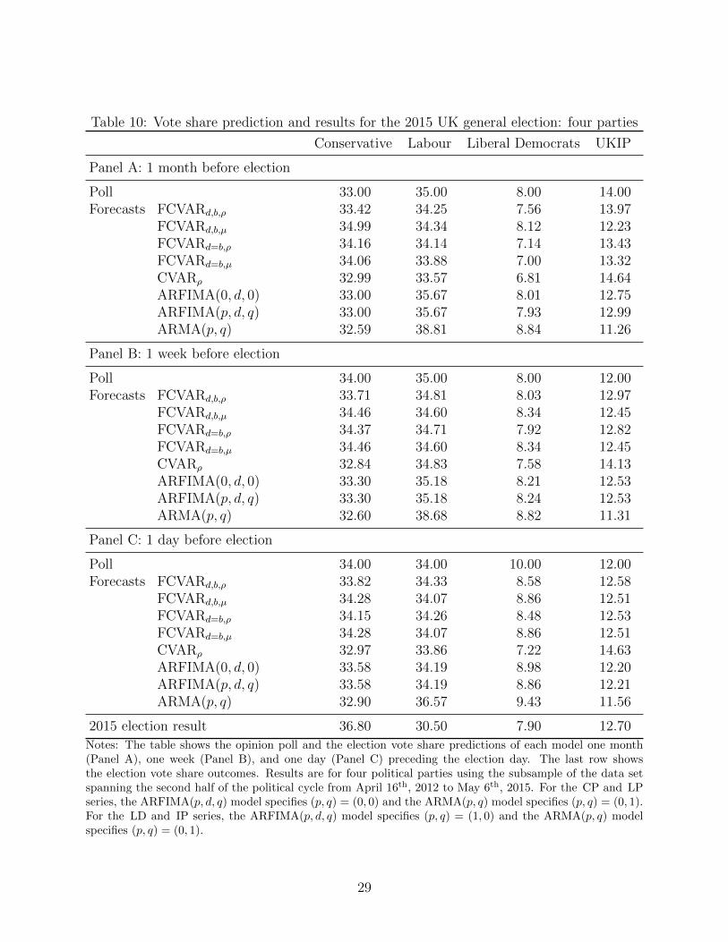
Table 10: Vote share prediction and results for the 2015 UK general election: four parties

Conservative Labour Liberal Democrats UKIP

Panel A: 1 month before election

Poll 33.00 35.00 8.00 14.00Forecasts FCVARd,b,ρ 33.42 34.25 7.56 13.97

FCVARd,b,µ 34.99 34.34 8.12 12.23FCVARd=b,ρ 34.16 34.14 7.14 13.43FCVARd=b,µ 34.06 33.88 7.00 13.32CVARρ 32.99 33.57 6.81 14.64ARFIMA(0, d, 0) 33.00 35.67 8.01 12.75ARFIMA(p, d, q) 33.00 35.67 7.93 12.99ARMA(p, q) 32.59 38.81 8.84 11.26

Panel B: 1 week before election

Poll 34.00 35.00 8.00 12.00Forecasts FCVARd,b,ρ 33.71 34.81 8.03 12.97

FCVARd,b,µ 34.46 34.60 8.34 12.45FCVARd=b,ρ 34.37 34.71 7.92 12.82FCVARd=b,µ 34.46 34.60 8.34 12.45CVARρ 32.84 34.83 7.58 14.13ARFIMA(0, d, 0) 33.30 35.18 8.21 12.53ARFIMA(p, d, q) 33.30 35.18 8.24 12.53ARMA(p, q) 32.60 38.68 8.82 11.31

Panel C: 1 day before election

Poll 34.00 34.00 10.00 12.00Forecasts FCVARd,b,ρ 33.82 34.33 8.58 12.58

FCVARd,b,µ 34.28 34.07 8.86 12.51FCVARd=b,ρ 34.15 34.26 8.48 12.53FCVARd=b,µ 34.28 34.07 8.86 12.51CVARρ 32.97 33.86 7.22 14.63ARFIMA(0, d, 0) 33.58 34.19 8.98 12.20ARFIMA(p, d, q) 33.58 34.19 8.86 12.21ARMA(p, q) 32.90 36.57 9.43 11.56

2015 election result 36.80 30.50 7.90 12.70

Notes: The table shows the opinion poll and the election vote share predictions of each model one month(Panel A), one week (Panel B), and one day (Panel C) preceding the election day. The last row showsthe election vote share outcomes. Results are for four political parties using the subsample of the data setspanning the second half of the political cycle from April 16th, 2012 to May 6th, 2015. For the CP and LPseries, the ARFIMA(p, d, q) model specifies (p, q) = (0, 0) and the ARMA(p, q) model specifies (p, q) = (0, 1).For the LD and IP series, the ARFIMA(p, d, q) model specifies (p, q) = (1, 0) and the ARMA(p, q) modelspecifies (p, q) = (0, 1).

29

Figure 5: Forecasts over 50 polling days leading into the election: three parties

(a) Forecasts of logit transformed series

2015-03-10 2015-05-0632

33

34

35

36

37CP

2015-03-10 2015-05-0630

32

34

36LP

2015-03-10 2015-05-066

7

8

9

10LD

2015-03-10 2015-05-06-0.9

-0.8

-0.7

-0.6

-0.5CP

FCVARd=b,ρ FCVARd=b,µ FCVARd,b,ρ FCVARd,b,µ

2015-03-10 2015-05-06-1

-0.9

-0.8

-0.7

-0.6

LP

2015-03-10 2015-05-06-3

-2.5

-2LD

2015-03-10 2015-05-0630

32

34

36

38CP

2015-03-10 2015-05-0630

35

40LP

2015-03-10 2015-05-067

8

9

10LD

2015-03-10 2015-05-06-1

-0.8

-0.6

-0.4

-0.2CP

CVARρ

ARFIMA(p, d, q) ARMA(p, q)

2015-03-10 2015-05-06-1

-0.8

-0.6

-0.4

-0.2LP

2015-03-10 2015-05-06-3

-2.5

-2

-1.5LD

Opinion Poll Election Result

(b) Forecasts of vote shares in percentage

2015-03-10 2015-05-0632

33

34

35

36

37CP

2015-03-10 2015-05-0630

32

34

36LP

2015-03-10 2015-05-066

7

8

9

10LD

2015-03-10 2015-05-06-0.9

-0.8

-0.7

-0.6

-0.5CP

FCVARd=b,ρ FCVARd=b,µ FCVARd,b,ρ FCVARd,b,µ

2015-03-10 2015-05-06-1

-0.9

-0.8

-0.7

-0.6

LP

2015-03-10 2015-05-06-3

-2.5

-2LD

2015-03-10 2015-05-0630

32

34

36

38CP

2015-03-10 2015-05-0630

35

40LP

2015-03-10 2015-05-067

8

9

10LD

2015-03-10 2015-05-06-1

-0.8

-0.6

-0.4

-0.2CP

CVARρ

ARFIMA(p, d, q) ARMA(p, q)

2015-03-10 2015-05-06-1

-0.8

-0.6

-0.4

-0.2LP

2015-03-10 2015-05-06-3

-2.5

-2

-1.5LD

Opinion Poll Election Result

Notes: Each subfigure shows the evolution of forecasts by different models variants for the May 7th, 2015general election. Panel (a) shows forecasts of logit transformed series, where 90% confidence bands areshown using with slightly thinner lines, and Panel (b) shows forecasts of vote shares in percentage. Theforecasts are calculated starting with the data available 50 polling days prior to the election and continueto May 6th, 2015, the day before the election. The results use the full data set spanning the entire politicalcycle (May 14th, 2010 to May 6th, 2015).

30

Figure 6: Forecasts over 50 polling days leading into the election: four parties

(a) Forecasts of logit transformed series

2015-03-10 2015-05-0632

33

34

35

36

37CP

2015-03-10 2015-05-0630

31

32

33

34

35

36LP

2015-03-10 2015-05-065

6

7

8

9

10LD

2015-03-10 2015-05-0611

12

13

14

15

16IP

2015-03-10 2015-05-06-0.9

-0.8

-0.7

-0.6

-0.5

-0.4CP

2015-03-10 2015-05-06-0.9

-0.8

-0.7

-0.6

-0.5LP

2015-03-10 2015-05-06-3

-2.8

-2.6

-2.4

-2.2

-2LD

2015-03-10 2015-05-06-2.4

-2.2

-2

-1.8

-1.6

-1.4IP

2015-03-10 2015-05-0632

33

34

35

36

37CP

2015-03-10 2015-05-0630

32

34

36

38

40LP

2015-03-10 2015-05-066

7

8

9

10LD

2015-03-10 2015-05-0611

12

13

14

15

16IP

2015-03-10 2015-05-06-0.9

-0.8

-0.7

-0.6

-0.5CP

2015-03-10 2015-05-06-1

-0.8

-0.6

-0.4

-0.2LP

CVARρ ARFIMA(p, d, q) ARMA(p, q)

2015-03-10 2015-05-06-3.2

-3

-2.8

-2.6

-2.4

-2.2

-2LD

FCVARd=b,ρ FCVARd=b,µ FCVARd,b,ρ FCVARd,b,µ

2015-03-10 2015-05-06-2.5

-2

-1.5

-1IP

Opinion Poll Election Result

(b) Forecasts of vote shares in percentage

2015-03-10 2015-05-0632

33

34

35

36

37CP

2015-03-10 2015-05-0630

31

32

33

34

35

36LP

2015-03-10 2015-05-065

6

7

8

9

10LD

2015-03-10 2015-05-0611

12

13

14

15

16IP

2015-03-10 2015-05-06-0.9

-0.8

-0.7

-0.6

-0.5

-0.4CP

2015-03-10 2015-05-06-0.9

-0.8

-0.7

-0.6

-0.5LP

2015-03-10 2015-05-06-3

-2.8

-2.6

-2.4

-2.2

-2LD

2015-03-10 2015-05-06-2.4

-2.2

-2

-1.8

-1.6

-1.4IP

2015-03-10 2015-05-0632

33

34

35

36

37CP

2015-03-10 2015-05-0630

32

34

36

38

40LP

2015-03-10 2015-05-066

7

8

9

10LD

2015-03-10 2015-05-0611

12

13

14

15

16IP

2015-03-10 2015-05-06-0.9

-0.8

-0.7

-0.6

-0.5CP

2015-03-10 2015-05-06-1

-0.8

-0.6

-0.4

-0.2LP

CVARρ ARFIMA(p, d, q) ARMA(p, q)

2015-03-10 2015-05-06-3.2

-3

-2.8

-2.6

-2.4

-2.2

-2LD

FCVARd=b,ρ FCVARd=b,µ FCVARd,b,ρ FCVARd,b,µ

2015-03-10 2015-05-06-2.5

-2

-1.5

-1IP

Opinion Poll Election Result

Notes: Each subfigure shows the evolution of forecasts by different models variants for the May 7th, 2015general election. Panel (a) shows forecasts of logit transformed series, where 90% confidence bands are shownusing slightly thinner lines, and Panel (b) shows forecasts of vote shares in percentage. The forecasts arecalculated starting with the data available 50 polling days prior to the election and continue to May 6th,2015, the day before the election. The results use the subsample of the data set spanning the second half ofthe political cycle (April 16th, 2012 to May 6th, 2015).

31

vote share for the UKIP. In particular, the CVAR model overshoots the election result forthe UKIP. For both the three-party and the four-party analyses, we find that the FCVARmodel predictions are on average closer to the realized vote shares than their analogs fromthe CVAR model.

The confidence bands in Figure 6(a) are broadly in agreement with those from Figure 5(a)for the Conservatives, Labour, and Liberal Democrats, with the exception that the univari-ate forecast bands now also exclude the election outcomes for the Conservatives and Labour.For the UKIP we find that the election result is within the confidence bands for all modelsthroughout the time period considered in the figure. However, noting the different scaling ofthe second axis for the IP plots for fractional and non-fractional models, respectively, it is ap-parent that the overprediction of the election result by the CVAR model is also accompaniedby a somewhat wider confidence band compared with the FCVAR model variants.

In general, the forecasting results from this empirical application show how modelingtime series of political opinion polls using the FCVAR model, which is strongly favored bythe model forecast comparisons, can complement the industry standard of basing predictionssolely on the most recent opinion poll (e.g., the poll standings on the day preceding the elec-tion day) and provide a more informative assessment of the current state of public opinion.Specifically, in the case of the 2015 UK general election, the FCVAR model forecasts provideadditional information on party support compared with the hung parliament prediction ofthe opinion poll.

6 Concluding remarks

This paper has examined the forecasting performance of the fractionally cointegrated vectorautoregressive (FCVAR) model of Johansen (2008) and Johansen and Nielsen (2012) relativeto a portfolio of competing models at several forecast horizons. The model was applied inthe context of predicting political support in the form of opinion polls; a very relevant topicin the context of forecasting. The analysis used a novel data set of daily polling of politicalsupport in the United Kingdom over the period 2010–2015. The analysis has shown howstatistical modeling of time series of public opinion polls can improve forecasting publicopinion beyond the most recent poll date. This complements the industry standard formeasuring the current state of political support through opinion polling, and contributes todecision making processes that rely on poll evidence as inputs.

Specifically, the forecasting analysis has shown that the FCVAR model delivers valuablegains in predicting political support. The accuracy of both short, medium, and long termforecasts generated by the FCVAR model is better than all multivariate and univariatemodels in the portfolio. Indeed, overall, the four variants of the FCVAR model are the topperforming models. Not only do they perform better relative to the other models, but theforecasting performance of all FCVAR model variants are within close range of each other.When compared to both the fractional benchmark model (ARFIMA) and the multivariatebenchmark model (CVAR), the FCVAR model significantly outperforms the benchmark atall forecast horizons and the gains are more pronounced at the longer forecast horizons, wherethe root mean squared forecast error is up to 15% lower than the fractional benchmark and20% lower than the multivariate benchmark. Overall, the evidence provides strong supportfor the application of the FCVAR model relative to both univariate fractional models andmultivariate non-fractional models. Fractional cointegration substantially improves forecast

32

accuracy, and the gains become more pronounced at longer forecast horizons.More generally, it is of interest to consider how generalizable our results are to other

data sets. The arguments in Section 2 certainly suggest that all polling data may be bestmodeled as fractional time series. This in turn suggests that the FCVAR model would beapplicable to all such data, and that the FCVAR model would produce superior forecasts forsuch data. In fact, the arguments in Section 2 suggest that our results may be generalizableto all data that have an aggregation structure, such as, in political science, any polling data,voting data, government support data, partisan indicators, etc. A thorough investigation ofwhether this is in fact the case is beyond the scope of this paper, and we leave this interestingissue for future research. However, we do note that the very general applicability of fractionalintegration models is in line with the literature, see e.g. Box-Steffensmeier and Tomlinson(2000) and Lebo et al. (2000).

In an empirical application to the 2015 UK general election, we have discussed the FCVARmodel estimation results, with interpretations of both the estimated cointegrating relationsand estimated common stochastic trend. It appears that the latter can be interpreted asa measure of Euro-skepticism, rather than an indicator of the more traditional left-rightpolitical spectrum, reflecting public opinion and debate in the sampling period which wasto a great extent focused on the European Union question. The forecasts generated by theFCVAR model leading into the election appear to provide a more informative assessment ofthe current state of public opinion on electoral support than the hung parliament predictionof the opinion polls. Specifically, when three political parties are modeled over the fullelection cycle, the FCVAR model predicts the correct direction for the realized vote sharesin the election for the Conservative and Labour parties. When four political parties aremodeled over the shorter available data set spanning the second half of the election cycle,the predictions of the FCVAR models are closer to the realized vote shares than their analogsfrom the CVAR model, and in particular the FCVAR models appear to converge more closelyto the realized vote share for the UKIP.

References

Baillie, R. T. (1996). Long memory processes and fractional integration in econometrics.Journal of Econometrics 73, 5–59.

Box, G. E. P. and G. M. Jenkins (1970). Time Series Analysis, Forecasting, and Control.San Francisco: Holden-Day.

Box-Steffensmeier, J. M. and R. M. Smith (1996). The dynamics of aggregate partisanship.American Political Science Review 90, 567–580.

Box-Steffensmeier, J. M. and A. R. Tomlinson (2000). Fractional integration methods inpolitical science. Electoral Studies 19, 63–76.

Byers, D., J. Davidson, and D. Peel (1997). Modelling political popularity: an analysis oflong-range dependence in opinion poll series. Journal of the Royal Statistical Society SeriesA 160, 471–490.

Byers, D., J. Davidson, and D. Peel (2000). The dynamics of aggregate political popularity:evidence from eight countries. Electoral Studies 19, 49–62.

Byers, D., J. Davidson, and D. Peel (2002). Modelling political popularity: a correction.Journal of the Royal Statistical Society Series A 165, 187–189.

33

Byers, D., J. Davidson, and D. Peel (2007). The long memory model of political support:some further results. Applied Economics 39, 2547–2552.

Dolado, J. J., J. Gonzalo, and L. Mayoral (2002). A fractional Dickey-Fuller test for unitroots. Econometrica 70, 1963–2006.

Dolado, J. J., J. Gonzalo, and L. Mayoral (2003). Long-range dependence in Spanish politicalopinion poll series. Journal of Applied Econometrics 18, 137–155.

Gonzalo, J. and C. W. J. Granger (1995). Estimation of common long-memory componentsin cointegrated systems. Journal of Business and Economic Statistics 13, 27–36.

Granger, C. W. (1980). Long memory relationships and the aggregation of dynamic models.Journal of Econometrics 14, 227–238.

Hualde, J. and P. M. Robinson (2011). Gaussian pseudo-maximum likelihood estimation offractional time series models. Annals of Statistics 39, 3152–3181.

Jensen, A. N. and M. Ø. Nielsen (2014). A fast fractional difference algorithm. Journal ofTime Series Analysis 35, 428–436.

Johansen, S. (1995). Likelihood-based inference in cointegrated vector autoregressive models.New York: Oxford University Press.

Johansen, S. (2008). A representation theory for a class of vector autoregressive models forfractional processes. Econometric Theory 24, 651–676.

Johansen, S. and M. Ø. Nielsen (2012). Likelihood inference for a fractionally cointegratedvector autoregressive model. Econometrica 80, 2667–2732.

Johansen, S. and M. Ø. Nielsen (2016). The role of initial values in conditional sum-of-squaresestimation of nonstationary fractional time series models. Econometric Theory 32, 1095–1139.

Jones, M. E., M. Ø. Nielsen, and M. K. Popiel (2014). A fractionally cointegrated VARanalysis of economic voting and political support. Canadian Journal of Economics 47,1078–1130.

Lebo, M. and H. D. Clarke (2000). Modelling memory and volatility: recent advances in theanalysis of political time series. Editor’s introduction. Electoral Studies 19, 1–7.

Lebo, M. J., R. W. Walker, and H. D. Clarke (2000). You must remember this: dealing withlong memory in political analyses. Electoral Studies 19, 31–48.

MacKinnon, J. G. and M. Ø. Nielsen (2014). Numerical distribution functions of fractionalunit root and cointegration tests. Journal of Applied Econometrics 29, 161–171.

Nielsen, M. Ø. (2015). Asymptotics for the conditional-sum-of-squares estimator in multi-variate fractional time series models. Journal of Time Series Analysis 36, 154–188.

Nielsen, M. Ø. and M. K. Popiel (2016). A Matlab program and user’s guide for the frac-tionally cointegrated VAR model. QED working paper 1330, Queen’s University.

Nielsen, M. Ø. and K. Shimotsu (2007). Determining the cointegrating rank in nonstationaryfractional systems by the exact local Whittle approach. Journal of Econometrics 141, 574–596.

Robinson, P. M. (1978). Statistical inference for a random coefficient autoregressive model.Scandinavian Journal of Statistics 5, 163–168.

Robinson, P. M. and Y. Yajima (2002). Determination of cointegrating rank in fractionalsystems. Journal of Econometrics 106, 217–241.

Shimotsu, K. and P. C. B. Phillips (2005). Exact local Whittle estimation of fractionalintegration. Annals of Statistics 33, 1890–1933.

34

Research Papers 2016

2016-14: Andrew J.G. Cairns, Malene Kallestrup-Lamb, Carsten P.T. Rosenskjold, David Blake and Kevin Dowd: Modelling Socio-Economic Differences in the Mortality of Danish Males Using a New Affluence Index

2016-15: Mikkel Bennedsen, Ulrich Hounyo, Asger Lunde and Mikko S. Pakkanen: The Local Fractional Bootstrap

2016-16: Martin M. Andreasen and Kasper Jørgensen: Explaining Asset Prices with Low Risk Aversion and Low Intertemporal Substitution

2016-17: Robinson Kruse, Christian Leschinski and Michael Will: Comparing Predictive Accuracy under Long Memory - With an Application to Volatility Forecasting

2016-18: Søren Johansen and Bent Nielsen: Tightness of M-estimators for multiple linear regression in time series

2016-19: Tim Bollerslev, Jia Li and Yuan Xue: Volume, Volatility and Public News Announcements

2016-20: Andrea Barletta, Paolo Santucci de Magistris and Francesco Violante: Retrieving Risk-Neutral Densities Embedded in VIX Options: a Non-Structural Approach

2016-21: Mikkel Bennedsen: Semiparametric inference on the fractal index of Gaussian and conditionally Gaussian time series data

2016-22: Søren Johansen and Morten Ørregaard Nielsen: The cointegrated vector autoregressive model with general deterministic terms

2016-23: Yunus Emre Ergemen and Carlos Vladimir Rodríguez-Caballero: A Dynamic Multi-Level Factor Model with Long-Range Dependence

2016-24: Shin Kanaya: Convergence rates of sums of α-mixing triangular arrays: with an application to non-parametric drift function

2016-25: Gustavo Fruet Dias, Marcelo Fernandes and Cristina M. Scherrer: Improving on daily measures of price discovery

2016-26: Martin M. Andreasen, Tom Engsted, Stig V. Møller and Magnus Sander: Bond Market Asymmetries across Recessions and Expansions: New Evidence on Risk Premia

2016-27: Kim Christensen, Ulrich Hounyo and Mark Podolskij: Testing for heteroscedasticity in jumpy and noisy high-frequency data: A resampling approach

2016-28: Kim Christensen, Roel Oomen and Roberto Renò: The Drift Burst Hypothesis

2016-29: Hossein Asgharian, Charlotte Christiansen, Rangan Gupta and Ai Jun Hou: Effects of Economic Policy Uncertainty Shocks on the Long-Run US-UK Stock Market Correlation

2016-30: Morten Ørregaard Nielsen and Sergei S. Shibaev: Forecasting daily political opinion polls using the fractionally cointegrated VAR model