Forecasting 1 Part

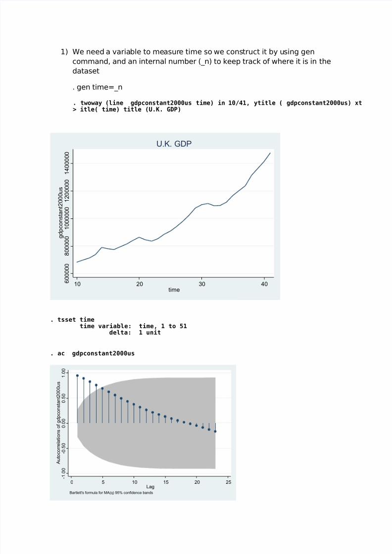
8/2/2019 Forecasting 1 Part

http://slidepdf.com/reader/full/forecasting-1-part 1/11

> itle( time) title (U.K. GDP). twoway (line gdpconstant2000us time) in 10/41, ytitle ( gdpconstant2000us) xt

1) We need a variable to measure time so we construct it by using gen

command, and an internal number (_n) to keep track of where it is in the

dataset

. gen time=_n

6 0 0 0 0 0

8 0 0 0 0 0

1 0 0 0 0 0 0

1 2 0

0 0 0 0

1 4 0 0 0 0 0

g d p c o n s t a n t 2 0 0 0

u s

10 20 30 40

time

U.K. GDP

delta: 1 unittime variable: time, 1 to 51

. tsset time

. ac gdpconstant2000us

- 1 . 0

0

- 0 . 5

0

0 . 0

0

0 . 5

0

1 . 0

0

A u t o c o r r e l a t i o n s o f g d p c o n s t a n t 2 0 0 0

u s

0 5 10 15 20 25Lag

Bartlett's formula for MA(q) 95% confidence bands



. pac gdpconstant2000us

- 1 . 0

0

- 0 . 5

0

0 . 0

0

0 . 5

0

1 . 0

0

P a r t i a l a u t o c o r r e l a t i o n s o f g d p c o n s t a n t 2 0 0 0 u s

0 5 10 15 20 25Lag

95% Confidence bands [se = 1/sqrt(n)]

_cons 401217.8 27704.17 14.48 0.000 344638.3 457797.3time 22894.49 1021.536 22.41 0.000 20808.24 24980.75

gdpconstan~s Coef. Std. Err. t P>|t| [95% Conf. Interval]

Total 1.5153e+12 31 4.8881e+10 Root MSE = 53355Adj R-squared = 0.9418

Residual 8.5403e+10 30 2.8468e+09 R-squared = 0.9436Model 1.4299e+12 1 1.4299e+12 Prob > F = 0.0000

F( 1, 30) = 502.29Source SS df MS Number of obs = 32

. reg gdpconstant2000us time in 10/41

. redict double uhatlinear, residual

. twoway (line uhatlinear time) in 10/41, ytitle (residual) xtitle(time)

- 5 0 0 0 0

0

5 0 0 0 0

1 0 0 0 0 0

1 5 0 0 0 0

r e s i d u a l

10 20 30 40time

The residual plot makes clear what is happening; the linear trend isinadequate, because the actual trend is nonlinear.



To plot the fitted linear time trend and the actual values of the variable we

do:

> rend)> e) in 10/41, ytitle ( gdpconstant2000us) xtitle(time) title(U.K. GDP: linear t

. twoway (scatter gdpconstant2000us time, msize(vsmall)) (line rshatlinear tim

. predict double rshatlinear, xb

6 0 0 0 0 0

8 0 0 0 0 0

1 0 0 0 0 0

0

1 2 0 0 0 0 0

1 4 0 0 0 0 0

g d p c o n s t a n

t 2 0 0 0 u s

10 20 30 40time

GDP (constant 2000 US$) Linear prediction

U.K. GDP: linear trend

In order to fit a quadratic trend to the data we need first to create variable

time squared (time2) and then regress the dependent variable

gdpconstant2000us on time and time2.

_cons 713054.1 44533.78 16.01 0.000 621972.3 804135.9time2 551.9227 73.28849 7.53 0.000 402.0309 701.8145time -5253.566 3786.257 -1.39 0.176 -12997.33 2490.199


Total 1.5153e+12 31 4.8881e+10 Root MSE = 31565Adj R-squared = 0.9796

Residual 2.8895e+10 29 996379727 R-squared = 0.9809Model 1.4864e+12 2 7.4321e+11 Prob > F = 0.0000

F( 2, 29) = 745.91Source SS df MS Number of obs = 32

. reg gdpconstant2000us time time2 in 10/41

. gen time2=time^2

It can be seen that both the linear and quadratic terms are highly

significant. The coefficient of determination is almost 1.



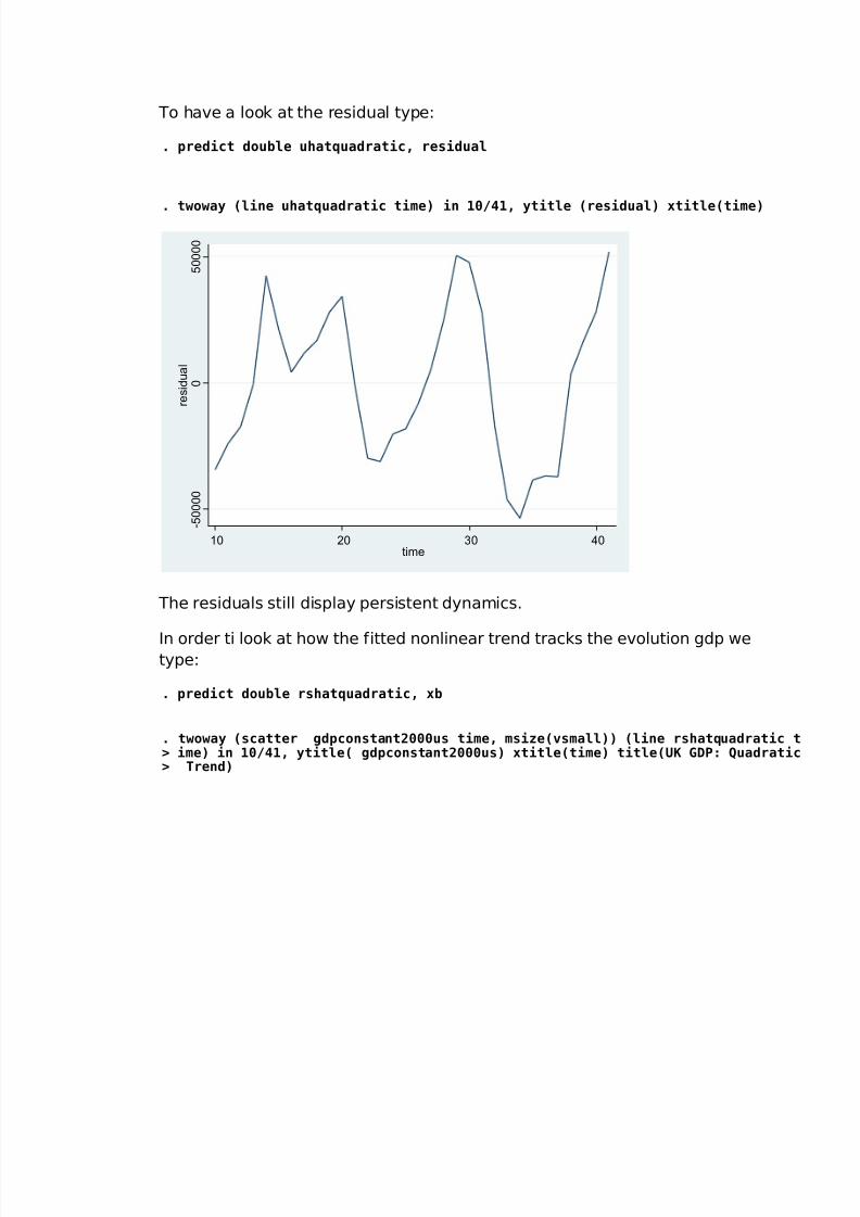
To have a look at the residual type:

. predict double uhatquadratic, residual

. twoway (line uhatquadratic time) in 10/41, ytitle (residual) xtitle(time)

- 5 0 0 0 0

0

5 0 0 0 0

r e s i d u a l

10 20 30 40time

The residuals still display persistent dynamics.

In order ti look at how the fitted nonlinear trend tracks the evolution gdp wetype:

. predict double rshatquadratic, xb

> Trend)> ime) in 10/41, ytitle( gdpconstant2000us) xtitle(time) title(UK GDP: Quadratic. twoway (scatter gdpconstant2000us time, msize(vsmall)) (line rshatquadratic t



6 0 0 0 0 0

8 0 0 0 0 0

1 0 0 0 0 0 0 1 2

0 0 0 0 0 1 4 0 0 0 0 0

g d p c o n s t a n t 2 0 0 0 u s

10 20 30 40time


UK GDP: Quadratic Trend

We need to estimate a different type of nonlinear trend model such as the

exponential trend. Here we need to create the variable log of gdp (lggdp)

and regress it on a constant and a time trend variable.

.

_cons 13.34497 .0415005 321.56 0.000 13.26009 13.42985time2 .0002734 .0000683 4.00 0.000 .0001337 .0004131time .009054 .0035284 2.57 0.016 .0018377 .0162703

lggdp Coef. Std. Err. t P>|t| [95% Conf. Interval]

Total 1.48161074 31 .047793895 Root MSE = .02942

Adj R-squared = 0.9819Residual .025092898 29 .000865272 R-squared = 0.9831

Model 1.45651784 2 .728258922 Prob > F = 0.0000F( 2, 29) = 841.65

Source SS df MS Number of obs = 32

. reg lggdp time time2 in 10/41

. gen lggdp=ln( gdpconstant2000us)

The estimation results show that the exponential nonlinear trend model

seems to feet well.

In order to look at the residuals:

. twoway (line uhatloglinear time) in 10/41, ytitle(residual) xtitle(time)

. predict double uhatloglinear, residual



- .

0 4

- .

0 2

0

. 0 2

. 0 4

. 0 6

r e s i d u a l

10 20 30 40time

In sharp contrast to the results of fitting a linear time trend to gdp, which

were poor, the results of fitting a time trend to the log of gdp seen much

improved.

. predict double rshatloglinear, xb

> 1, ytitle ( gdpconstant2000us) xtitle(time) title(U.K. GDP: Long Linear Trend). twoway (scatter lggdp time, msize(vsmall)) (line rshatloglinear time) in 10/4



1 3 .

4

1 3 .

6

1 3 .

8

1 4

1 4 .

2

g d p c o n s t a n t 2 0 0 0 u s

10 20 30 40time

lggdp Linear prediction

U.K. GDP: Long Linear Trend

It is hard to compare the log-linear trend-model with the linear and

quadratic models because they are in levels (no logs), which renders

diagnostic statistics that are incomparable. One way around this problem is

to estimate the exponential trend model directly in levels, using nonlinear

least squares.

/b1 .0239659 .0007537 31.80 0.000 .0224266 .0255051/b0 521484.5 12065.97 43.22 0.000 496842.5 546126.5


Total 3.2564e+13 32 1.0176e+12 Res. dev. = 762.7827Root MSE = 37489.31

Residual 4.2163e+10 30 1.4054e+09 Adj R-squared = 0.9986Model 3.2522e+13 2 1.6261e+13 R-squared = 0.9987

Number of obs = 32Source SS df MS

Iteration 5: residual SS = 4.22e+10Iteration 4: residual SS = 4.22e+10Iteration 3: residual SS = 4.22e+10Iteration 2: residual SS = 9.54e+10Iteration 1: residual SS = 5.40e+11Iteration 0: residual SS = 1.52e+12

(obs = 32). nl ( gdpconstant2000us={b0}*exp({b1}*time)) in 10/41

To look at residuals:

. twoway (line uhatexponential time) in 10/41, ytitle (residual) xtitle(time)

. predict double uhatexponential, residual



- 5 0 0 0 0

0

5 0 0

0 0

1 0 0 0 0 0

r e s i d u a l

10 20 30 40time

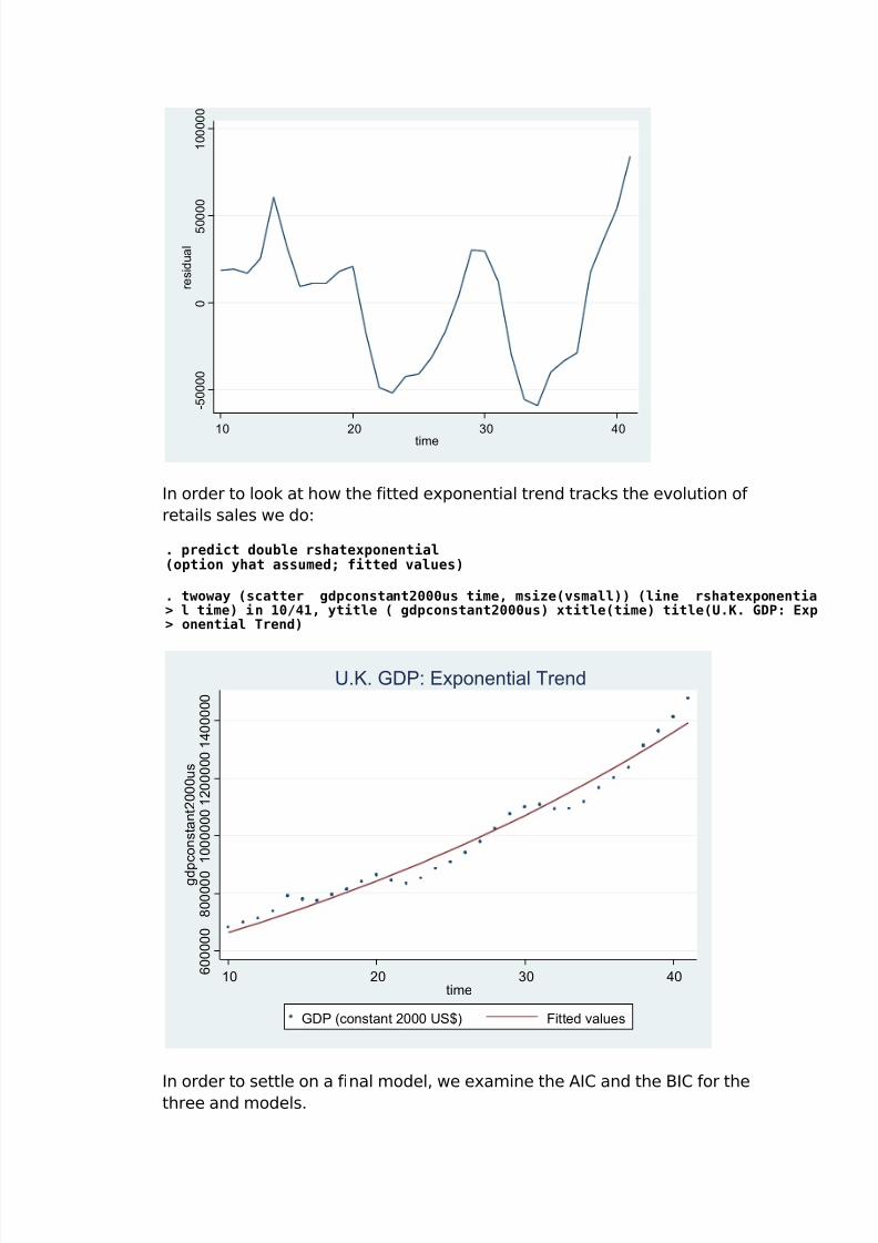
In order to look at how the fitted exponential trend tracks the evolution of

retails sales we do:

(option yhat assumed; fitted values). predict double rshatexponential

> onential Trend)> l time) in 10/41, ytitle ( gdpconstant2000us) xtitle(time) title(U.K. GDP: Exp. twoway (scatter gdpconstant2000us time, msize(vsmall)) (line rshatexponentia

6 0 0 0 0 0

8 0 0 0 0 0

1 0 0 0 0 0 0 1 2 0 0 0 0 0 1 4 0 0 0 0 0

g d p c o n s t a n t 2 0 0 0 u s

10 20 30 40time

GDP (constant 2000 US$) Fitted values

U.K. GDP: Exponential Trend

In order to settle on a final model, we examine the AIC and the BIC for thethree and models.



_cons 401217.8 27704.17 14.48 0.000 344638.3 457797.3time 22894.49 1021.536 22.41 0.000 20808.24 24980.75


Total 1.5153e+12 31 4.8881e+10 Root MSE = 53355

Adj R-squared = 0.9418Residual 8.5403e+10 30 2.8468e+09 R-squared = 0.9436

Model 1.4299e+12 1 1.4299e+12 Prob > F = 0.0000F( 1, 30) = 502.29


. reg gdpconstant2000us time in 10/41

bic 792.30069aic 789.36922

_cons 401217.8time 22894.492

Variable active

. estimates table, stats(aic bic)

_cons 713054.1 44533.78 16.01 0.000 621972.3 804135.9time2 551.9227 73.28849 7.53 0.000 402.0309 701.8145time -5253.566 3786.257 -1.39 0.176 -12997.33 2490.199


Total 1.5153e+12 31 4.8881e+10 Root MSE = 31565

Adj R-squared = 0.9796Residual 2.8895e+10 29 996379727 R-squared = 0.9809

Model 1.4864e+12 2 7.4321e+11 Prob > F = 0.0000F( 2, 29) = 745.91





/b1 .0253559 .0004748 53.41 0.000 .0244018 .02631/b0 508319.8 9191.855 55.30 0.000 489848.1 526791.6


Total 6.4286e+13 51 1.2605e+12 Res. dev. = 1242.286Root MSE = 48066.58

Residual 1.1321e+11 49 2.3104e+09 Adj R-squared = 0.9982Model 6.4173e+13 2 3.2086e+13 R-squared = 0.9982

Number of obs = 51Source SS df MS

Iteration 5: residual SS = 1.13e+11Iteration 4: residual SS = 1.13e+11

Iteration 3: residual SS = 1.13e+11Iteration 2: residual SS = 1.24e+11Iteration 1: residual SS = 4.70e+12Iteration 0: residual SS = 7.69e+12

(obs = 51). nl( gdpconstant2000us={b0}*exp({b1}*time))

bic 1250.15aic 1246.2864

Statistics

_cons .02535592b1

_cons 508319.83b0

Variable active

. estimates table, stats(aic bic)

According to our results we chose quadratic trend model, because it has the

lowest AIC and BIC.

_cons 713054.1 44533.78 16.01 0.000 621972.3 804135.9time2 551.9227 73.28849 7.53 0.000 402.0309 701.8145time -5253.566 3786.257 -1.39 0.176 -12997.33 2490.199


Total 1.5153e+12 31 4.8881e+10 Root MSE = 31565

Adj R-squared = 0.9796Residual 2.8895e+10 29 996379727 R-squared = 0.9809

Model 1.4864e+12 2 7.4321e+11 Prob > F = 0.0000F( 2, 29) = 745.91



. gen low=rshatquadratic-1.96*e(rmse)

. gen high=rshatquadratic+1.96*e(rmse)



> ( gdpconstant2000us) xtitle(time) title(U.K. GDP). twoway (line gdpconstant2000us rshatquadratic low high time) in 41/51, ytitle

1 4 0 0 0 0 0

1 6 0 0 0 0 0

1 8 0 0 0 0 0

2 0 0 0 0 0 0

g d p c o n s t a n t 2 0 0 0 u s

40 45 50time


low high

U.K. GDP

Forecasting 1 Part

Documents

Transcript of Forecasting 1 Part