California Energy Commission Edmund G. Brown Jr., Governor

April 2018 | CEC-200-2018-005

California Energy Commission

FINAL CONSULTANT REPORT

Forecast of Medium- and Heavy-Duty Vehicle Attributes to 2030

Prepared for: California Energy Commission Prepared by: H-D Systems

California Energy Commission

DISCLAIMER This report was prepared as the result of work sponsored by the California Energy Commission. It does not necessarily represent the views of the Energy Commission, its employees, or the State of California. The Energy Commission, the State of California, its employees, contractors, and subcontractors make no warrant, express or implied, and assume no legal liability for the information in this report; nor does any party represent that the uses of this information will not infringe upon privately owned rights. This report has not been approved or disapproved by the California Energy Commission nor has the California Energy Commission passed upon the accuracy or adequacy of the information in this report.

Primary Author(s):

Gopal Duleep H-D Systems 4417 Yuma St. NW Washington DC (202)-966-0286 www.h-dsytems.com Contract Number: 800-16-005

Prepared for:

California Energy Commission

Sudhakar Konala Contract Manager

Bob McBride Project Manager

Siva Gunda Office Manager DEMAND ANALYSIS OFFICE

Sylvia Bender Deputy Director ENERGY ASSESSMENTS DIVISION Drew Bohan Executive Director

i

ABSTRACT

This California Energy Commission report documents the forecast of vehicle fuel

economy and price for medium- and heavy-duty vehicles for the 2016-to-2030 period

and the technological and modeling assumptions used to derive the forecast. The Energy

Commission uses transportation energy demand models that require projections of

these vehicle attributes. The fuel economy and greenhouse gas emissions of medium-

and heavy-duty vehicles are required to meet specific mandated levels by federal

regulations through 2027 and beyond. Since the standards necessitate the use of more

fuel-saving technologies than would otherwise be demanded by the market, the

regulatory analysis developed by United States Environmental Protection Agency and

National Highway Traffic Safety Administration (in support of the standards) is used

extensively, though some modifications were made to derive the projections for the

Energy Commission. This report also summarizes the technologies available to improve

the fuel economy of trucks powered by conventional gasoline or diesel engines, as well

as those using alternative fuels like ethanol, natural gas, electricity, and hydrogen. H-D

Systems developed projections for two scenarios in this analysis.

Keywords: California Energy Commission, vehicle attributes, heavy-duty trucks,

attribute forecast, fuel economy, alternative fuels

Duleep, Gopal. (H-D Systems), 2017. Forecast of Medium- and Heavy-Duty Vehicle

Attributes to 2030. California Energy Commission. Publication Number:

CEC-200-2018-005.

ii

iii

TABLE OF CONTENTS

ABSTRACT ............................................................................................................................................. i

Table of Contents ............................................................................................................................... iii

List of Figures ..................................................................................................................................... iv

List of Tables ....................................................................................................................................... iv

EXECUTIVE SUMMARY ....................................................................................................................... 1

CHAPTER 1: Introduction ................................................................................................................. 3

CHAPTER 2: Vehicle Classes Used in Forecast ............................................................................ 5 Weight Classes ................................................................................................................................. 5 Alternative Fuels and the Energy Commission’s Class/Fuel Matrix ..................................... 6 Cross-Classification Matrix ........................................................................................................... 9

CHAPTER 3: Technology to Improve Heavy-Duty Vehicle Fuel Economy ........................... 11 Overview ......................................................................................................................................... 11 Diesel Engines ............................................................................................................................... 11 Gasoline Engines........................................................................................................................... 15 Natural Gas Engines ..................................................................................................................... 16 Transmissions and Axles............................................................................................................ 17 Aerodynamics ............................................................................................................................... 18 Improved Rolling Resistance ..................................................................................................... 20 Weight Reduction ......................................................................................................................... 21 Hybrid Drivetrains ....................................................................................................................... 23 Electric Vehicles ............................................................................................................................ 25 Summary ........................................................................................................................................ 27

CHAPTER 4: Forecast of Heavy-Duty Vehicle Attributes ........................................................ 31 U.S. EPA/NHTSA Standards ........................................................................................................ 31 Forecast of Vehicle Prices ........................................................................................................... 36 Forecasts ........................................................................................................................................ 37

LIST OF ACRONYMS......................................................................................................................... 47

ATTACHMENT I: H-D Systems (EEA) Report to Department Of Energy on Heavy-Duty

Truck Fuel Economy ........................................................................................................................ 49

iv

LIST OF FIGURES Page

Figure 2-1: CARB HHDDT Transient Cycle .................................................................................... 9

LIST OF TABLES Page

Table 2-1: Operating Duty Cycle for Vocational Vehicles .......................................................... 6

Table 2-2: California Energy Commission Vehicle Class and Fuel Type Matrix .................... 7

Table 2-3: EPA Duty Cycle Mix ...................................................................................................... 10

Table 2-4: Cross-Classification Matrix ......................................................................................... 10

Table 3-1: Cost Estimates for a Class 8 Diesel, Catenary, Electric, and Fuel Cell Truck in

Volume Production in 2020 ........................................................................................................... 27

Table 3-2: Vehicle Technologies (Costs in 2027) ....................................................................... 29

Table 4-1: RIA Estimates for 2021 Fuel Economy by Class (Reproduced From RIA) ........ 32

Table 4-2: RIA Estimates for 2024 Fuel Economy by Class (Reproduced From RIA) ........ 33

Table 4-3: RIA Estimates for 2027 Fuel Economy by Class (Reproduced From RIA) ........ 34

Table 4-4: RIA Estimates for 2021 to 2027 Fuel Economy – Custom Chassis (Reproduced

From RIA) ........................................................................................................................................... 35

Table 4-5: Forecast Vehicle Attribute Data Worksheet for High-Electricity Demand Case ...

..................................................................................................................................................... 39

Table 4-6: Forecast Vehicle Attribute Data Worksheet for Low-Electricity Demand Case ...

....................................................................................................................................................... 43

1

EXECUTIVE SUMMARY The California Energy Commission estimates fuel consumption in the transportation

sector and projects the market penetration of alternative fuel vehicles as a part of the

2017 Integrated Energy Policy Report and other state projects. To forecast these values,

the Energy Commission uses transportation demand models that require projections of

vehicle attributes for the 2016-to-2030 period. This report presents H-D Systems’

forecast of medium- and heavy-duty vehicle fuel economy and vehicle prices, which are

used as inputs into the Energy Commission’s transportation models. The report also

documents the technological and modeling assumptions used to derive the attribute

forecast.

The second phase of the federal Greenhouse Gas Emissions and Fuel Efficiency Standards

for Medium- and Heavy-Duty Engines and Vehicles require medium- and heavy-duty

vehicles to meet specific mandated fuel economy levels through 2027. The United States

Environmental Protection Agency and the National Highway Traffic Safety

Administration completed a comprehensive analysis of technological improvements

available to improve fuel economy and reduce greenhouse gas emissions in support of

the Federal Phase 2 regulations. The analysis by the agencies is documented in the

Regulatory Impact Assessment of the federal Phase 2 standards. H-D Systems’ forecast

of vehicle attributes for the Energy Commission uses many elements of the standards

derived in the Regulatory Impact Assessment.

The Energy Commission’s transportation demand models require medium- and heavy-

duty attributes by vehicle class and fuel type. Medium- and heavy-duty trucks are

classified into six industry weight classes (Classes 3 to 8), and the Energy Commission

subdivides Class 8 trucks by vocation. Furthermore, the Energy Commission classifies

buses as urban transit buses, shuttle buses, school buses, and motor coaches. Finally,

the fuel types requested by the Energy Commission include:

• Gasoline-electric hybrid.

• Diesel-electric hybrid.

• Diesel-hydraulic hybrid.

• Battery-electric.

• Direct or catenary electric.

• Fuel cell electric.

• Ethanol (E85).

• Compressed natural gas.

• Liquefied natural gas.

• Propane.

In general, gasoline and diesel engines are common in smaller (Classes 3 to 5) trucks,

while heavier vehicles are typically powered by diesel engines. In the highest weight

classes, diesel engines are used in more than 95 percent of all trucks. Hence, the focus

2

of the analysis starts with diesel-powered vehicles, while alternative powertrains are

considered relative to diesel.

To generate forecasts of fuel economy, H-D Systems considered several fuel efficiency

technologies in this analysis, including:

• Improvements in engine efficiency and reduction of losses in the engine,

transmissions, and axles.

• A reduction in vehicle weight, aerodynamic drag, or tire-rolling resistance.

The technologies available and the respective costs and benefits are summarized in this

report.

This report provides forecasts for two scenarios. The first is a high electricity demand

case that assumes electric vehicles are successful and uses the high-volume production

forecast to generate electric vehicle prices. The second is a low electricity demand case

that uses the current (low-volume production) prices of electric vehicles and assumes

manufacturers are able to achieve cost reductions through increasing manufacturing

experience but not of scale for the forecast. This scenario also uses the high transit bus

prices from the California Air Resources Board as the starting point for prices in 2017

and assumes benefits of learning but not of scale for the forecast. The forecasts project

that for all internal combustion engine-powered vehicles from 2017 to 2030

• Vehicles in Classes 3 and 4 (mostly large pickups and vans) will increase fuel

economy by about 25 to 29 percent.

• Medium-duty trucks in Classes 6 and 7 that operate in mixed suburban and

urban routes will increase fuel economy by 22 to 25 percent.

• Vehicles in mostly urban use like garbage trucks and urban buses will have

improvements in fuel economy of 9 to 12 percent.

• Long-haul trucks in Classes 7 and 8 will see the largest improvement of 29 to 32

percent in fuel economy.

Electrical vehicles in each class will see smaller improvements in fuel efficiency because

the electric motor is already very efficient and future gains in efficiency will be small;

hence, most of the efficiency improvement is associated with improvements to body

technology. Costs of electric vehicles, however, are forecast to decline mostly due to

battery cost reduction and improved economies of scale.

3

CHAPTER 1: Introduction The California Energy Commission’s Transportation Energy Forecasting Unit (TEFU) has

a set of transportation energy demand models that require forecasts of medium- and

heavy-duty vehicle attributes (fuel economy and price) from 2016 to 2030. The models

are used by TEFU to estimate future fuel consumption and the market penetration of

alternative fuel vehicles, which help inform the 2017 Integrated Energy Policy Report

(IEPR) and provide analytical support for implementing state policy goals. This report

documents the forecast of medium- and heavy-duty vehicle fuel economy and price, and

the technological and modeling assumptions used to derive the forecast.

The fuel economy and greenhouse gas (GHG) emissions of medium- and heavy-duty

vehicles are required to meet specific mandated levels by the federal Greenhouse Gas

Emissions and Fuel Efficiency Standards for Medium- and Heavy-duty Engines and

Vehicles for the 2010-to-2017 period. They have recently been extended to the 2018-to-

2027 period by the “Phase 2” regulations. The standards require a high level of effort

from heavy-duty vehicle manufacturers and essentially make the future fuel economy

levels for each vehicle weight class virtually independent of future fuel prices unless

prices rise to unanticipated levels. Fuel prices could still affect the mix of vehicle weight

classes and fuel types sold, but for a given weight class and fuel type, fuel economy

improvements are forced by standards rather than economics.

The way to meet the fuel economy standards is by improving the technology of trucks.

A comprehensive analysis of technological improvements has been completed by the

United States Environmental Protection Agency (U.S. EPA) and the National Highway

Traffic Safety Administration (NHTSA) in support of the 2014-2017 Phase 1 and 2018-

2027 Phase 2 regulations. The analysis builds on earlier work on heavy-duty vehicle

technology by the U.S. EPA, National Academy of Sciences (NAS), and H-D Systems (HDS).

The forecast relies on technologies being added to a known baseline (2017) of vehicle

characteristics. The more recent work by U.S. EPA/NHTSA is documented in the

Regulatory Impact Assessment (RIA) released in 2016,1 and this forecast uses many

elements of the standards derived in the RIA. Since the standards are technology-

forcing,2 the analysis in the RIA is used extensively with some modification to derive the

forecast for the Energy Commission.

Chapter 2 of this report describes the weight classes and fuel types used by the Energy

Commission and maps the Commission’s vehicle class definitions to those used by the

EPA and NHTSA. In addition to the weight class and fuel type classifications, trucks in

the same weight classes are used in applications with different use-based duty cycles.

1 U.S. EPA/NHTSA. August 2016. Greenhouse Gas Emissions and Fuel Efficiency Standards for Medium- and Heavy-Duty Vehicles, Regulatory Impact Assessment, EPA Report 420-R-16-900. 2 ”Technology forcing” refers to regulations that require (force) the use of more technology than demanded by the free market to achieve performance standards.

4

The Energy Commission’s weight class by application is matched to the appropriate

duty cycle definitions used in the RIA.

Chapter 3 summarizes the technology analysis in the RIA and provides a listing of the

technologies used to improve fuel economy. Based on earlier HDS analysis of medium-

and heavy-duty technology for the U.S. Department of Energy (DOE),3 aspects of the RIA

that H-D Systems believes overstate on-road fuel economy potential of some

technologies are corrected for in the forecast developed for the Energy Commission, and

these corrections are described. HDS’ analysis for DOE is provided as an attachment to

this report. The Energy Commission’s forecast also requires data for battery-electric,

fuel cell electric, and direct electric drive vehicles, which are not covered in the RIA, and

HDS’ assumptions are documented in this section.

Chapter 4 summarizes HDS’ forecast, which is similar to the EPA/NHTSA forecast except

for the correction to some of the technology benefits employed by EPA and NHTSA. The

forecasts in the RIA (from which the HDS forecasts are derived) are shown in this

section, and the forecasts developed for the Energy Commission are listed.

The attached supplement (the DOE report) also provides some limited historical data on

medium- and heavy-duty truck fuel economy derived from the 2002 Vehicle Inventory

and Use Survey (2002 VIUS)4 and other data sources. VIUS was known as the Truck

Inventory and Use Survey, or TIUS, before 1997.

3 EEA/ICF. December 2011. Technological Potential to Reduce Heavy-Duty Truck Fuel Consumption to 2025, report to the DOE Office of Policy. 4 Found at www.census.gov/svsd/www/vius/2002.html.

5

CHAPTER 2: Vehicle Classes Used in Forecast

Weight Classes The California Energy Commission’s transportation energy demand models require

medium- and heavy-duty vehicle attributes by vehicle weight class and fuel type.

Medium- and heavy-duty trucks are generally classified by industry weight Classes 3 to

8, and the class definitions, as well as the typical vehicle types in each class, are

provided below.

Weight Classes 3, 4, and 5 are referred to as light heavy-duty (LHD) trucks by the

automotive industry and EPA (but as medium-duty by the Energy Commission) and span

the 10,000-to-19,000 pound gross vehicle weight (GVW) range. Class 3 consists mostly

of pickup trucks and cargo vans, like the Ford F-350 and Dodge D-3500, as well as a few

small size “cabover” Japanese trucks. Classes 4 and 5 are increasingly dominated by the

Japanese models, although pickup trucks like the Ford F-450 and 550 have significant

market share. Vehicle sales in this class are about 70 percent diesel and 30 percent

gasoline. Trucks in this class are used for light commercial activity like plumbing, lawn

maintenance, and utility support, while the Japanese trucks are used typically for local

pickup and delivery.

Weight Classes 6 and 7 are referred to as medium heavy-duty (MHD) trucks and span the

19,000-to-33,000 pound GVW range. These classes are dominated by conventional two-

axle straight trucks and were almost completely diesel-powered, although Ford

reintroduced gasoline-powered models in the last two years in response to high diesel

fuel prices. Trucks in this class are used for urban pickup and delivery, as well as

suburban and rural freight distribution. A significant fraction of these vehicles are

vocational trucks used by local gas and electric utilities and by city services.

Class 8, which is referred to as heavy heavy-duty (HHD) trucks, is usually split into two

subclasses, 8A and 8B. Trucks in Class 8A are typically three-axle trucks covering the

35,000-to-55,000-pound weight range and include trucks used in construction and waste

disposal, as well as suburban and rural freight distribution. Class 8B trucks are four-

and five-axle trucks in the 60,000-to-80,000 pound weight range, with the majority of

these trucks devoted to medium- (between 100 and 500 miles) and long-haul (greater

than 500 miles) freight distribution. Heavy construction trucks, tanker trucks, and

specialized vocational trucks have a smaller share of the 8B market. Trucks in Class 8A

and 8B are usually diesel-powered.

Motorhomes and buses – including school buses, transit buses, and long-haul coaches –

are derived from truck chassis. School buses and small motorhomes are typically Class

5 or 6 (depending on length) and are about 60 percent diesel-powered, with gasoline and

alternative fuels like compressed natural gas (CNG) or propane used in many buses.

Large motorhomes, transit buses, and motor coaches are in the 30,000-to-35,000-pound

6

GVW range (that is, Class 7 or 8A) and are usually diesel–powered, although a significant

portion of transit buses use compressed (CNG) or liquefied (LNG) natural gas.

The RIA provides an overview of the use type for all vocational vehicles; these data from

Table 2-65 of the RIA are shown in Table 2-1. Long-haul Class 8 trucks operate more

than 80 percent of total miles on highways. Multipurpose driving involves a mix of city

and urban highway driving, while regional driving is on suburban and state highway

routes.

Table 2-1: Operating Duty Cycle for Vocational Vehicles REGIONAL MULTIPURPOSE URBAN

Class 4-5 straight truck 9% 41% 50%

Class 6-7 straight truck 15% 50% 35%

Class 8 straight truck 20% 60% 20%

Long haul Class 6 to 8 straight truck, motorhome

100% 0% 0%

School Bus 0% 10% 90%

Transit Bus 0% 0% 100%

Refuse truck 0% 10% 90%

Source: U.S. EPA/NHSTA RIA. Figures are percentages of VMT.

Alternative Fuels and the Energy Commission’s Class/Fuel Matrix The Energy Commission’s Truck Choice model estimates market share by vehicle weight

class, vocation, and fuel type. The truck fuel types modeled by the Energy Commission

include the:

• Gasoline-electric hybrid.

• Diesel-electric hybrid.

• Diesel-hydraulic hybrid.

• Battery–electric.

• Direct or catenary electric.

• Fuel cell electric.

• Ethanol (E85).

• Compressed natural gas (CNG).

• Liquefied natural gas (LNG).

• Propane.

7

Not all combinations of fuel types and weight classes are expected to be introduced into

the market. Hence, a matrix of expected combinations was agreed upon by H-D Systems

and Energy Commission staff, and the combinations are shown in Table 2-2.

Table 2-2: California Energy Commission Vehicle Class and Fuel Type Matrix

# CEC Vehicle Class Gas

oli

ne

Gas

oli

ne

Ele

ctri

c H

yb

rid

Die

sel

Die

sel

Ele

ctri

c H

yb

rid

Die

sel

Hy

dra

uli

c H

yb

rid

Bat

tery

-Ele

ctri

c V

eh

icle

s

Dir

ect

(Cat

en

ary

) Ele

ctri

c Fu

el C

ell

Veh

icle

s

E8

5 (

eth

os

engin

e)

Com

pre

ssed

Nat

ura

l G

as

(CN

G)*

Liq

uef

ied

Nat

ura

l gas

(L

NG

)*

Pro

pan

e (L

PG

)

GVWR 3 GVWR 3 O O O P P O A A

GVWR 4 to 6

GVWR 4 O O O P A O O A A

GVWR 5 O O A O O A

GVWR 6 O P P O A

GVWR 7 & 8

GVWR 7 O P A

GVWR 8 Single Unit

O

A A

GVWR 8 Combination (California)

O P A A

GVWR 8 Garbage O O A A A

GVWR 8 Combination (Interstate)

O O O

Motorhomes GVWR 3 O O

GVWR 4 to 6 O O A

Bus

Urban Transit O O A P O P A

Motor Coach O

School Bus O

O P A A

Shuttle Bus O

A O

A A

Source: California Energy Commission and H-D Systems O – Original Equipment Manufacturer P – Pilot Production** A – Aftermarket * Includes Low NOx engines. ** Pilot production refers to production of less than 100 units per year.

8

H-D Systems’ Observations on Truck Availability by Fuel Type The low oxides of nitrogen (NOx) natural gas engine was included in the standard

natural gas category as it is a transient product for the 2018-2022 time frame (after

2022, HDS expects all natural gas trucks to have low NOx natural gas engines).

Gasoline electric hybrids are not offered in Classes 3 to 5 but may be offered in 2019

and later years as full-size pickup manufacturers plan to introduce hybrids in the light-

duty versions of these pickups that have similar bodies and drivetrains. Diesel hybrids

have also been recently introduced into the market by select Japanese manufacturers in

Classes 5 and 6 trucks.

Hydraulic hybrids do not appear to be under serious consideration by truck

manufacturers but are available as aftermarket conversions by manufacturers such as

Bosch-Rexroth and Parker Hannifin. Both series and parallel types are offered, but

because of lower costs, HDS has included only the series type in the forecast as an

aftermarket product.

Electric vehicles of many types are expected to be introduced into the market. Two

Asian manufacturers, BYD and Fuso, are offering battery-electric vehicles in Classes 5, 6,

and 7, while there is pilot production of transit and school buses. (Pilot production is a

term used in this report to refer to production of fewer than 100 units per year.) Electric

trucks operating like trolleys with a catenary but also having a battery for short-range

unconnected use are also being discussed, with a pilot program underway in the South

Coast Air Quality Management District. Fuel cell trucks are not yet available, although

there is pilot production of fuel cell buses.

E85 vehicles are available directly from manufacturers of Classes 3, 4, and 5 gasoline-

powered trucks and are sold as gasoline- and E85-compatible flex-fuel vehicles. CNG

vehicles and propane vehicles in these classes are aftermarket conversions of gasoline

vehicles (not diesel engines), as no manufacturer offers alternative fuel vehicles directly,

but some like Ford have “qualified” aftermarket suppliers. In 2015, one manufacturer

(Cummins-Westport) offered a 6.6 liter diesel engine conversion to CNG suitable for this

market, but anecdotal evidence suggests only minor sales in markets for Classes 4 and 5

trucks. Aftermarket gasoline engine conversions to CNG also have modest sales,

accounting for less than 1 percent of Classes 3, 4, and 5 sales nationally.

CNG and LNG vehicles in Classes 6, 7, and 8A use specially converted diesel engines,

and there is only one supplier for these engines – Cummins-Westport, which provides

the 6.6 liter and 9 liter engines. CNG and LNG have found significant market penetration

in the urban transit bus market and in garbage trucks, where local or state regulations

sometimes require the use of natural gas. Westport introduced a compression ignition

natural gas engine for the Class 8B market but withdrew it in 2014 due to poor sales. A

new 12 liter Cummins-Westport spark ignition engine suitable for this market was

introduced in 2016. All the available diesel engine-based conversions use spark ignitions

for CNG and are less energy-efficient than the comparable power diesel engine.

9

Cross-Classification Matrix

The Energy Commission’s weight classifications and vehicle types are not the same as

the EPA/NHTSA-based vehicle use type and weight classes, and a mapping between the

two classifications is required to translate the regulatory requirements applicable to

each Energy Commission class.

The translation is based upon an understanding of the class-specific duty cycles used by

EPA for testing the vehicles for compliance. EPA has settled on using three test cycles

and two idle tests for assessing compliance, and class-specific figures are determined by

different weightings of each cycle used to construct a composite figure. The three test

cycles are the 65 mph steady-state cruise, the 55 mph steady-state cruise, and the

California Air Resources Board (CARB) transient test. The cruise tests for the 2018-2027

Phase 2 standards involve simulation of road gradients, whereas the same cruise modes

for the Phase 1 standards did not have any gradient. The CARB transient test, shown as

a speed-time trace in Figure 2-1, represents typical urban driving and includes some

higher speed portions in the 40-to-50-mph range that occurs along major arterials and

urban highways. The two idle modes are in parked and drive (transmission engaged)

modes, respectively. Each truck type class is assigned a mix of the five modes to derive

the composite fuel economy and GHG emissions standard.

Figure 2-1: CARB HHDDT Transient Segment

Source: Diesel.net (www.dieselnet.com/standards/cycles/index.php).

The EPA specified duty cycle mix from Tables 3-16 and 3-19 of the RIA, according to the

related classification, is shown below. The nonidle modes add to 100 percent.

10

Table 2-3: EPA Duty Cycle Mix

Transient 55 mph 65 mph Idle

Drive

Idle-

Park

Vocational Regional 20% 24% 56% 0% 25%

Vocational

Multipurpose

54% 29% 17% 17% 25%

Vocational

Multipurpose (Class 8)

54% 23% 23% 17% 25%

Vocational Urban 92% 8% 0% 15% 25%

Regional Day Cab 19% 17% 64% NA NA

Long Haul (Sleeper) 5% 9% 86% NA NA

Source: U.S. EPA/NHSTA RIA. Percentages are in terms of VMT, except for idle, which is in percentage of operating

time.

Based on these considerations, HDS developed a cross-classification matrix, as shown in

Table 2-3, mapping the Energy Commission’s medium- and heavy-duty vehicle classes to

the EPA truck regulatory categories

Table 2-4: Cross-Classification Matrix CEC Class EPA Regulatory Category

GVWR 3 LHD Multipurpose

GVWR 4 LHD Multipurpose

GVWR 5 LHD Multipurpose

GVWR 6 MHD Multipurpose

GVWR 7 MHD Regional

GVWR 8 Single Unit HHD multipurpose

GVWR8 Combination (California) Class 8 Mid-roof Day cab

Garbage Refuse Truck

GVWR8 IRP (Combination) Class 8 High Roof Sleeper cab

GVWR 3 motorhome LHD Regional

GVWR 4 to 6 motorhome Motorhome

GVWR 7 & 8 motorhome MHD regional

Urban Transit Transit bus

Motor Coach Coach bus

School Bus School bus

Source: H-D Systems.

11

CHAPTER 3: Technology to Improve Heavy-Duty Vehicle Fuel Economy

Overview Diesel engines power the majority of heavy-duty vehicles and are used in more than 95

percent of all trucks in the highest weight classes. Hence, the focus of the analysis is on

diesel-powered vehicles, with all other alternatives considered relative to diesel. Fuel

efficiency technologies can be broadly separated into those that improve the efficiency

by which energy in a fuel is converted to motive power, and by those that reduce the

power demand to travel a specific distance. Technologies affecting the former are those

that improve engine efficiency and reduce losses in the engine, transmission, and axles.

Technologies affecting power demand are those that reduce the weight, aerodynamic

drag, or tire-rolling resistance. In the case of trucks, some operational factors like

limiting cruise speed or preventing extended idle can improve fuel consumption. The

technologies available and the related costs and benefits in both categories are

summarized below. The analysis is based on the detailed RIA from the U.S. EPA/NHTSA.

Electric vehicles change the entire drivetrain but still benefit from power demand

reductions. All the data and fuel efficiency estimates cited in this chapter are from the

RIA unless specifically stated otherwise.

Diesel Engines EPA and NHTSA considered available diesel engine technologies that could improve

engine fuel efficiency. A detailed description of each technology can be found in H-D

Systems’ report on truck fuel economy, which was created for the U.S. Department of

Energy and is included as an attachment to this report. The technologies considered

were

• Combustion system optimization.

• Model-based control.

• Advances to turbocharging systems.

• Engine air handling systems improvement.

• Parasitic and friction loss reduction.

• After-treatment integration.

• Downsizing and downspeeding.

12

Combustion System Optimization Combustion system optimization, featuring piston bowl, injector tip, and the number of

holes, in conjunction with the advanced fuel injection system, is able to improve engine

performance and fuel efficiency. Examples include the combustion development

programs conducted by diesel engine manufacturers funded by the U.S. Department of

Energy as part of the Super Truck program. The manufacturers found improvement due

to combustion alone was 1 to 2 percent. The agencies determined that it is feasible that

fuel consumption could be reduced by as much as 1.0 percent in the agencies’

certification cycles in the 2027 time frame by using these technologies.

Some technologies such as homogeneous charge compression ignition, premixed charge

compression ignition (PCCI), low-temperature combustion, and reactivity-controlled

compression ignition technologies were not included in the agencies’ feasibility analysis,

as they were unlikely to be commercialized by 2027.

Model-Based Control Another important area of potential improvement is advanced engine control

incorporating model-based calibration to reduce losses of control during transient

operation, that is, when operating at varying speeds. Improvements in computing power

and speed would make it possible to use more sophisticated algorithms that are more

predictive than today’s controls. Detroit Diesel recently introduced the next-generation

model-based control concept, achieving 4 percent thermal efficiency improvement while

reducing emissions in transient operations. More recently, this model-based control

technology was put into one of the vehicles for final demonstration under DOE’s Super

Truck program.

The model-based concept features a series of real-time optimizers5 with

multiple inputs and outputs. Real-time model control could be in production during the

2017-2027 time frame, thus significantly improving engine fuel economy.

Advances to the Turbocharging System Many advanced turbocharger technologies are available in the time frame between

Model Years 2021 and 2027, and some of them are already in production, such as the

mechanical or electric turbo-compound, the higher-efficiency variable-geometry turbine,

and the asymmetric turbocharger.

A turbo-compound system extracts energy from the exhaust to provide additional power.

Mechanical turbo-compounding includes a power turbine located downstream of the

turbine, which, in turn, is connected to the crankshaft to supply additional power. It was

first used in heavy-duty production by Detroit Diesel, which claims a 3 to 5 percent fuel

consumption reduction due to the system, while Volvo reports a 2 to 4 percent

improvement.

Results depend on the duty cycle and require significant time at high load

to see an improvement in fuel efficiency. Light load-factor vehicles can expect little or

no benefit. Electric turbo-compound is another potential technology that can improve

5 Engine control is optimized for the actual operating cycling of the engine as it occurs, which depends on factors such as the age of the engine.

13

engine brake efficiency. Since the electric power turbine speed is no longer linked to

crankshaft speed, this allows more efficient operation of the turbine. Navistar reports

on the order of a 1 to 1.6 percent efficiency improvement over mechanical turbo-

compound systems. This concept, however, does not work well with lower engine

emissions due to lower exhaust gas temperatures.

Two-stage turbocharger technology has been used in production by Navistar and other

manufacturers. Ford’s newly developed 6.7 liter diesel engine features a twin-

compressor turbocharger. Higher boost with a wider range of operations and higher

efficiency can enhance engine performance and, thus, fuel economy. It is expected that

this type of technology will continue to be improved by better matching with system

requirements and developing higher compressor and turbine efficiency.

Engine Air-Handling System Various high-efficiency air-handling (air and exhaust transport) processes could be

produced with efficiently designed flow paths (including those associated with air

cleaners, chambers, conduit, mass airflow sensors, and intake manifolds) and by

designing such systems for improved thermal control. Improved turbocharging and air

handling systems must include higher-efficiency exhaust gas recirculation (EGR)

systems and intercoolers that reduce pressure loss while maximizing the ability to

thermally control induction air and EGR. Other components that offer opportunities for

improved flow efficiency include cylinder heads, ports, and exhaust manifolds to

further reduce pumping losses. Manufacturers report a 1.4 percent to 2 percent fuel

efficiency improvement through air-handling system development.

Navistar predicts

almost 4 percent improvement through a combination of variable intake valve closing

timing, which may include a partial Miller cycle,6 as well as turbocharger efficiency and

match improvements.

Engine Parasitic and Friction Reduction Engine parasitic7 and friction reduction is another key technical area that can be

improved in the 2020-to-2027 time frame. Reduced friction in bearings, valve trains, and

the piston-to-liner interface can improve efficiency. Friction reduction opportunities in

the engine valve train and at the roller/tappet interfaces exist for several production

engines. The piston at the skirt/cylinder wall interface, wrist pin, and oil ring/cylinder

wall interface offers opportunities for friction reduction. More advanced lubricating oil

will be available in the future and will play a key role in reducing friction. Lube oil and

water pumps are another area where efficiency improvements are planned.

Manufacturers report 2 to 3 percent reductions in fuel consumption from a combination

of improvements to friction and water/oil pump improvements. Water pump

improvements include pump efficiency improvement and variable-speed or on/off

6 The Miller cycle is a thermodynamic cycle used in a type of internal combustion engine, where fuel is combusted to extract useful mechanical energy. It is a variant of the standard Otto/Diesel cycle that improves performance at partial (or less than maximum) engine load. 7 Engine parasitic losses are energy losses due to vehicle accessories such as the oil and water pumps.

14

controls. Lube pump improvements are primarily achieved using variable displacement

pumps and may include efficiency improvement. EPA contractor reports show that if the

exact certification cycles, weighting, and vehicle weights are used, the friction reduction

in the Phase 2 time frame is in the range of 1.5 percent compared to a 2018 baseline

engine.

Integrated Aftertreatment System All manufacturers now use diesel particulate filters to reduce particulate matter (PM)

and selective catalytic reduction (SCR) to reduce NOx emissions, and these types of

aftertreatment technologies are likely to be used for compliance with criteria pollutant

standards for many years to come. There are three areas considered to improve

integrated aftertreatment systems, which result in a reduction of fuel consumption. The

first is better combustion system optimization through increased aftertreatment

efficiency. The second is reduced back pressure (the pressure in an exhaust pipe due to

restriction of air flow that an engine must work against) through further development of

the devices themselves. The third is reduced ammonia slip, or unreacted ammonia, out

of SCR during transient operation, thus reducing net urea consumption. Cummins

reports a 0.5 percent improvement through improved aftertreatment flow. Detroit

Diesel projects a 2 percent fuel efficiency improvement through reduced use of EGR,

thinner wall diesel particulate filters, improved SCR cell density, and catalyst material

optimization8.

Engine Downsizing and Downspeeding Engine downsizing9 can be more effective if it is combined with downspeeding10 when

total power demand is reduced. This lower power demand shifts the vehicle operating

points to lower load zones, which moves the engine operating point to a less efficient

area. Downspeeding allows the engine to move back into the optimum operating points,

resulting in reduced fuel consumption. Detroit Diesel also shows that engine

downsizing can result in friction reduction due to a reduction in engine surface area

when compared to a bigger bore engine.

Engine downspeeding can also be an effective fuel efficiency technology even when used

alone (that is, not in combination with engine downsizing), especially when a vehicle

uses a fast axle ratio. In this situation, downspeeding can allow the engine to operate in

a lower speed zone closer to or just in the middle of the optimal efficiency operating

point of the engine. On the other hand, from a vehicle operating standard point, the

benefit of downspeeding is realized primarily by using a lower axle ratio, allowing the

engine to operate in an optimal zone.

8 Catalyst material optimization is the selection of catalytic material to optimize emissions reductions of particulate matter and NOx. 9 Engine downsizing represents the reduction the engine size with no loss in power. 10 Engine operation at lower RPM to reduction friction losses and operate the engine at a lower fuel consumption point.

15

Waste Heat Recovery

Organic Rankine cycle waste heat recovery (WHR) systems have been under development

for decades, but performance and cost issues have prevented commercialization. The

basic approach of a WHR system is to use engine exhaust waste heat from multiple

sources to evaporate a working fluid in a heat exchanger. This evaporated fluid is then

passed through a turbine or equivalent expander to create mechanical or electrical

power. The working fluid is then condensed back to the fluid in the fluid reservoir tank

and returned to the flow circuit via a pump to restart the cycle.

With support of the U.S. Department of Energy, three major engine and vehicle

manufacturers have developed WHR systems under the Super Truck program.11 The

agencies recognize the many challenges that would need to be overcome but believe

with enough time and development effort, this can be done. Manufacturers have stated

that the WHR systems in the literature and used in the DOE Super Truck program are

still in the research and development stage and are a long way from reaching

production. The U.S. EPA and NHTSA have been optimistic and have included WHR

systems in their forecast. HDS does not estimate that the WHR will be cost–effective,

and EPA’s own estimates show that the cost is more than $1,500 per 1 percent

improvement in fuel consumption, which is significantly higher than those for other

technologies. While the agencies project a 5 percent market penetration in 2024 and 25

percent market penetration in 2027 for WHR, HDS has set it to zero. This constitutes the

only major difference in the diesel engine technology forecast from the 2027 forecast in

the RIA.

Gasoline Engines The U.S. EPA and NHTSA did not set aggressive standards for gasoline engines as they

believed that the 2016 standard overstated the performance of actual 2016 gasoline

engines. Many technologies developed for use with light-duty pickup trucks are also

available for the light heavy-duty class. The most prominent technologies are:

• Direct injection with increased compression ratio.

• Engine friction and parasitic loss reduction.

• Variable-cylinder management (or cylinder cut).

• Downsizing and downspeeding.

The number of engine families in the light heavy-duty vehicle segment is relatively few

(about six) and are derived mostly from light-duty V8 engines. (Ford has a V10 engine.)

As of 2017, all employ port fuel injection and conversion to direct injection, like many

of their light-duty counterparts, where a one-unit increase in compression ratio can

provide fuel consumption reduction of 2 to 2.5 percent.

11 The Super Truck program is a U.S. DOE program to test advanced truck technology.

16

Engine friction and parasitic loss reduction uses technologies similar to those described

for diesel and offer a 1 to 1.5 percent fuel consumption reduction over the next 10

years. Cylinder-cut technology is widely employed in light-duty V8 engines and some

light-heavy V8 models, but the benefit in fuel consumption is smaller than for light-duty

vehicles, since the engines are more heavily loaded. The benefit for light-duty engines is

about 6 percent, while in the light heavy-duty segment, it falls to about 3 percent.

Downsized turbocharged engines are less likely in the light heavy-duty segment as such

engines offer no benefit over naturally aspirated engines at high loads. As a result, HDS

agrees with the U.S. EPA/NHTSA position that such engines will have limited penetration

in the Classes 3 to 5 vehicle segments. Downsizing and downspeeding are closely

related to turbocharging and increasing engine specific power, so that the impact of

these technologies will also be limited, except to the extent made possible by

transmission changes.

The net benefit of all technological improvements is in the 6 to 7 percent range but

some engines feature cylinder cut technology in 2017, and not all engines will receive all

technology improvements by 2027, especially in the absence of forcing standards.

Hence, we estimate a net average fuel consumption reduction of 4 to 5 percent between

2017 and 2027, which is quite similar to the benefits forecast from diesel engine

improvements over the same time frame.

Natural Gas Engines As noted in Chapter 2, CNG engines for the light heavy-duty segment are usually

conversions of gasoline engines in the aftermarket. (The

“aftermarket” refers to modifications made to a vehicle after purchase by a third party

and not the manufacturer.) These conversions do not change the basic engine

calibrations or hardware but add gas injectors to provide a stoichiometric mixture of

air-fuel to the engine. The net result is usually no significant change in the energy

efficiency of natural gas engines relative to the unconverted gasoline engine, in terms of

vehicle energy consumption per mile.

Natural gas engines used in Classes 6, 7, and 8A trucks are conversions of diesel engines

to gasoline (or spark ignition) engines. These engines feature turbocharging and have a

relatively high compression ratio; so they are more efficient than conventional gasoline

engines but still significantly less efficient than comparable diesel engines. The engines

operate at a stoichiometric air-fuel ratio that allows the use of a cheaper emission

control system to meet standards relative to the complex system used in a diesel engine.

The RIA suggests that these engines are about 15 percent less fuel-efficient than a diesel

engine over the same duty cycle.

While the only natural gas engine available for Class 8B trucks today is also a spark

ignition engine, there have been examples of natural gas engines in limited production

that more closely resemble diesel-cycle engines and use a small amount of diesel fuel

for a pilot injection to initiate combustion. However, the emission control system is as

17

expensive as the one used for diesel engines, and the two fuel systems result in higher

engine costs and complexity. Fuel efficiency is expected to be only 3 to 5 percent worse

than a comparable diesel engine, according to the RIA. Such engines could be introduced

into the market in 2018 or 2019.

Transmissions and Axles Transmissions and axles are part of the drivetrain, and ways to improve transmissions

include electronic controls, shift strategy, gear efficiency, and gear ratios. The relative

importance of having an efficient transmission increases when vehicles operate in

conditions with a higher shift density. Each shift represents an opportunity to lose

speed or power that would have to be regained after the shift is completed. Further,

each shift engages gears that have inherent inefficiencies. Optimization of the vehicle

gearing to engine performance through selection of transmission gear ratios, final drive

gear ratios, and tire size can play a significant role in reducing fuel consumption and

GHGs. Optimization of gear selection versus vehicle and engine speed accomplished

through driver training or automated transmission gear selection can provide additional

reductions.

Manufacturers of light and medium heavy-duty vehicles can replace six-speed

transmissions with eight-speed or more automatic transmissions. Additional ratios

allow for optimizing engine operation over a wider range of conditions, but this is

subject to diminishing returns as the number of speeds increases. Also, the additional

shifting of such a transmission can be perceived as bothersome to some consumers, so

manufacturers need to develop strategies for smooth shifts. The RIA rulemaking

projected that eight-speed transmissions could incrementally reduce fuel consumption

by 2 to 3 percent from a baseline six-speed automatic transmission over some test

cycles. The efficiency of gears can be improved by reducing friction and minimizing

mechanical losses. During operation, the controller of an automatic transmission

manages the transmission by scheduling the upshift or downshift, and locking or

allowing the torque converter to slip based on a preprogrammed shift schedule. This

aggressive shift logic12 can be employed to maximize fuel efficiency by modifying the

shift schedule13 to upshift earlier and inhibit downshifts under some conditions,

allowing the engine to operate at higher efficiency points.

The manual transmission has traditionally been more efficient than automatic

transmissions, and advances in electronics and computer processing power allow for

more efficiency from a manual transmission architecture with fully automated shifting.

The two primary manual transmission architectures employing automated shifting are

the automated manual transmission (AMT) and the dual-clutch transmission. When

implemented well, these more mechanically efficient designs provide better fuel

efficiency than conventional automatic transmission designs and, potentially, even fully

12 Aggressive shift logic refers to maximizing fuel economy by forecasting when transmission shift changes may be needed. 13 The shift schedule refers to when a transmission shift change is scheduled to occur.

18

manual transmissions. An AMT is mechanically similar to a conventional manual

transmission, but shifting and launch functions are automatically controlled by

electronics. The term AMT generally refers to a single-clutch design (differentiating it

from a dual-clutch transmission), which is essentially a manual transmission with

automated clutch and shifting. Because of shift quality issues with single-clutch designs,

dual-clutch designs are more common in light-duty applications, where driver

acceptance is of primary importance. For heavy-duty vehicles, shift quality remains

important but is less so when compared to light-duty vehicles. As a result, the single-

clutch AMT can be an attractive technology for heavy-duty vehicles and provides up to 2

percent fuel consumption reduction.

Axle efficiency is improved by reducing two categories of losses: mechanical losses (due

to friction) and spin losses (due to energy transfer to unwanted axle fluid churning or

spin). Mechanical losses can be reduced by reducing the friction between the two gears

in contact. Frictional losses are proportional to the torque on the axle but are not a

function of rotational speed of the axle. Spin losses, on the other hand, are a function of

speed, not torque. One of the main ways to reduce the spin losses of the axle is by using

a lower-viscosity lubricant. Some high-performance, lower-viscosity oil formulations

have been designed to have superior performance at high operating temperatures and

may have extended change intervals. Axle efficiency improvements can contribute up to

2 percent improvement in fuel consumption. In dual-rear-axle vehicles, using only one

axle for traction power reduces losses but can be traction limited under slippery

conditions. An axle-disconnect system allows the rear axle to be engaged as required

and provides a 1.5 percent gain in fuel economy.

Aerodynamics Up to 25 percent of the fuel consumed by a line-haul tractor traveling at highway speeds

is used to overcome aerodynamic drag forces, making aerodynamic drag a significant

contributor to the GHG emissions and fuel consumption of a Class 7 or 8 tractor.

Because aerodynamic drag varies by the square of the vehicle speed, small changes in

the tractor aerodynamics can have significant impacts on GHG emissions and fuel

efficiency of that vehicle. With much of the driving at highway speed, the benefits of

reduced aerodynamic drag for Class 7 or 8 tractors can be significant, but for vehicles

that operate primarily in urban areas and at low speed, aerodynamics are not a

significant factor in fuel consumption. The common measure of aerodynamic efficiency

is the coefficient of drag (Cd). The aerodynamic drag force (the force the vehicle must

overcome due to air) is a function of Cd, the area presented to the wind (the projected

area perpendicular to the direction of travel or frontal area) known as the drag area, and

the square of the vehicle speed. Cd values for today’s line-haul fleet typically range from

greater than 0.80 for a classic body tractor to about 0.58 for tractors that incorporate a

full package of widely commercially available aerodynamic features on both the tractor

and trailer.

19

Aerodynamic drag reduction is accompanied by smoothing the shape of the vehicle to

make it more aerodynamically efficient, redirecting air to prevent entry into areas of

high drag (for example, wheel wells), maintaining smooth air flow in certain areas of the

vehicle, or a combination of these. Improving the vehicle shape may include revising the

fore components of the vehicle such as rearward canting/raking or smoothing/rounding

the edges of the front-end components (for example, bumper, headlights, windshield,

hood, cab, mirrors) or integrating the components at key interfaces (for example,

windshield/glass to sheet metal) to alleviate vehicle drag. Finally, redirecting the air to

prevent low-pressure areas and eliminating areas where turbulent vortices are created

reduce drag. Techniques such as blocking gaps in the sheet metal, ducting of

components, shaping or extending sheet metal to reduce flow separation and turbulence

are methods being considered to direct air from areas of high drag (for example, the

underbody, tractor-trailer gap, underbody, or rear of trailer, or a combination of these).

The heavy-duty transport industry implemented significant aerodynamic refinements,

but improvements were integrated mostly into tractor bodies with no trailer

contribution. Most of the future aerodynamic improvement potential will come from

further refinement of the gap between tractor and trailer, underbodies, and the trailer

itself, and, to a much lesser extent, improvements in tractor aerodynamics. Operators

traditionally resisted aerodynamic trailer add-on technology because of cooling

problems, ground clearance, durability, and length limitations imposed on highway

trucks. The use of devices such as inflatable adjustable gap seals or retractable skirts (or

active devices) should reduce incompatibility issues but will be more difficult to justify

for add-on costs and reliability. The institutional trailer issues have been addressed in

the Phase 2 rulemaking for 2017 to 2027 to force the aerodynamic devices for trailers to

be actually implemented widely in the market.

The U.S. EPA/NHTSA rulemaking for Phase 1 standards had very similar data and

identified aerodynamic “packages” which were labeled as Bin 1 to Bin 10. Each bin

represents a combination of discrete technologies. Bin 1 is the baseline package with a

Cd of 0.79, consistent with HDS data for the “classic” tractor-trailer. EPA has defined

Bins 2, 3, and 4 packages in terms of values of 0.72, 0.63, and 0.56, respectively, for Cd. The technologies are generally defined but not specific, as manufacturers have to

evaluate the actual aerodynamic performance to compute the Cd x A parameter that

must fall within predefined values. EPA had also defined a Bin 5 with a Cd value of 0.51

for unspecified future improvements. In its Phase 2 rulemaking, EPA shifted the scale to

Cd x A units and specified levels for Bins 1 to 6 that are specific to each tractor type, but

generally follow the same principles invoked in the 2017 rulemaking.

The aerodynamic simulations for the RIA rely on the two constant speed cycles at 55

mph and 65 mph, respectively. HDS believes that the results overstate the importance of

aerodynamics for two reasons. First, most highways with significant freight traffic in

California are congested with frequent slowdowns. Even if the average speed is 55 mph

or 65 mph, the speedup and slowdown cycles increase energy use, and the fraction of

20

energy lost to aerodynamic drag becomes smaller. Second, the drag values are based on

a truck moving in an empty track and does not account for the other vehicles ahead of it

that reduce the drag due to the wake effect. Informal platooning of trucks is common

on highways as truckers try to capture this aerodynamic benefit at no cost. Data cited in

the DOE report in Appendix B suggest that at highway speeds, each 10 percent drag

reduction results in a fuel consumption improvement of 3.8 percent rather than 5.2

percent in EPA simulations. Hence, one change made to the U.S. EPA/NHTSA forecast is

the reduction of benefits from aerodynamic devices by 27 percent (in other words, 27%

= 100% - 3.8%/5.2%). This change affects the fuel economy of regional and long-haul use

trucks only.

Improved Rolling Resistance Research indicates that the contribution of a tire to overall vehicle fuel efficiency is

roughly proportional to the vehicle weight. Energy loss associated with tires is mainly

due to deformation of the tires under the load of the vehicle, known as hysteresis, but

smaller losses result from aerodynamic drag, and other friction forces between the tire

and road surface and the tire and wheel rim. Collectively, the forces that result in energy

loss from the tires are referred to as rolling resistance. Rolling resistance is a factor

considered in the design of the tire and is affected by the tread and casing compound

materials, the architecture of the casing, tread design, and the tire manufacturing

process. It is estimated that 35 to 50 percent of the rolling resistance of a tire is from

the tread, and the other 50 to 65 percent is from the casing. In addition to the effect on

fuel consumption, design and use characteristics of tires also influence durability,

traction, vehicle handling, ride comfort, and noise. Tires that have higher rolling

resistance likely represent a different trade-off with one or more of these other tire

attributes. Tire inflation can also affect rolling resistance in that under-inflated tires can

result in increased deformation and contact with the road surface.

According to an energy audit cited in the RIA, tires were shown to be the second largest

contributor to energy losses for a Class 6 delivery truck at 50 percent load and speeds

up to 35 mph (a typical average speed of urban delivery vehicles). For Class 8 tractor-

trailers, the share of vehicle energy required to overcome rolling resistance is estimated

at nearly 23 percent. On a cycle basis, the energy use attributed to tires varies from 20

to 35 percent, depending on weight class and duty cycle.

Differences in rolling resistance of up to 50 percent have been identified for tires

designed to equip the same vehicle. Low-rolling-resistance tires are commercially

available from most tire manufacturers and can be applied to vehicles in all medium-

and heavy-duty vehicle classes. Low-rolling-resistance tires can be offered for dual-

assembly tires and as wide-base singles.

Wide-base singles (WBS) are intended primarily for combination tractor-trailers, but

some vocational vehicles are able to accommodate them. In the early years of this

technology, some states and local governments restricted use of WBS, but many of these

21

restrictions have since been lifted. A wide-base single is a larger tire with a lower profile

that replaces two standard tires. Generally, a wide-base single tire has less sidewall

flexing compared to a dual assembly; therefore, less hysteresis occurs. Compared to a

dual-tire assembly, wide-base singles also produce less aerodynamic resistance or drag.

Wide-base singles can contribute to improving the fuel efficiency of a vehicle through

design as a low-rolling-resistance tire or through vehicle weight reduction or both. The

use of fuel-efficient wide-base singles can reduce rolling resistance by 3.7 to 4.9 percent

compared to the most equivalent dual tire. The data collected based on field testing

indicate that tractors equipped with wide-base singles on the drive axle experience

better fuel efficiency than tractors equipped with dual tires, independent of the type of

tire on the trailer. This field study in particular indicated a 6.2 percent improvement in

fuel efficiency from wide-base singles. There are also weight savings associated with

wide-base singles compared to dual tires. Wide-base singles can reduce the weight of a

tractor and trailer by as much as 1,000 pounds when combined with aluminum wheels.

Tire Inflation Monitoring and Maintenance Systems Proper tire inflation is critical to maintaining proper stress distribution in the tire, which

reduces heat loss and rolling resistance. Tires with reduced inflation pressure exhibit

more sidewall flexing and tread shearing, resulting in greater rolling resistance than a

tire operating at its optimal inflation pressure. Tractor-trailers operating with all tires

underinflated by 10 psi have been shown to increase fuel consumed by up to one

percent. Tires can gradually lose pressure from small punctures, leaky valves, or simply

diffusion through the tire casing. Changes in ambient temperature can also affect tire

pressure. Trailers that remain unused for long periods between hauls may experience

any of these conditions. To achieve the intended fuel efficiency benefits of low-rolling-

resistance tires, it is critical that tires are maintained at the proper inflation pressure.

Tire pressure monitoring (TPM) and automatic tire inflation (ATI) systems are designed

to address underinflated tires. Both systems alert drivers if tire pressure drops below

the set point. TPM systems monitor the tires and require user-interaction to reinflate to

the appropriate pressure. Unless the vehicle experiences a catastrophic tire failure,

simply alerting the driver that the tire pressure is low may not necessarily result in

reinflation as the driver may continue driving to the destination before addressing the

tires. Current ATI systems take advantage of air brake systems of trailers to supply air

back into the tires (continuously or on demand) until a selected pressure is achieved. In

the event of a slow leak, ATI systems have the added benefit of maintaining enough

pressure to allow the driver to get to a safe stopping area. The RIA estimates the fuel

consumption reduction due to TPM and ATI systems to be 1 and 1.2 percent,

respectively.

Weight Reduction Weight reduction is a technology that can be used in a manufacturer’s strategy to meet

the Phase 2 standards. Vehicle weight reduction (also referred to as “light-weighting”)

decreases fuel consumption by reducing the energy demand needed to overcome inertia

22

forces and rolling resistance. Reduced weight in heavy-duty vehicles can benefit fuel

efficiency and reduce carbon dioxide (CO2) emissions in two ways. If a truck is running

at the gross vehicle weight limit with high-density freight, more freight can be carried on

each trip, increasing the payload efficiency of the truck in ton-miles per gallon. If the

vehicle is carrying lower density freight and is below the GVWR (or gross combination

weight of the tractor and trailer) limit, the total vehicle mass is decreased, reducing

rolling resistance and the power required to accelerate or climb grades.

Although many gains have been made to reduce vehicle mass, many of the new features

being added to modern tractors to benefit fuel efficiency, such as additional

aerodynamic features or idle reduction systems, increase vehicle mass, causing the total

mass to stay relatively constant. Hybrid powertrains, fuel cells, and auxiliary power

would not only present complex packaging and weight issues; they would increase the

need for reductions in the weight of the body, chassis, and powertrain components to

maintain vehicle functionality.

Substitution of a material used in an assembly or a component for one with lower

density or higher strength or both includes replacing a common material such as mild

steel with higher-strength and advanced steel, aluminum, magnesium, and composite

materials. It is the typical method to reduce weight. In practice, material substitution

tends to be specific to the manufacturer and situation. The agencies recognized that like

any type of mass reduction, material substitution has to be conducted not only with

consideration to maintaining equivalent component strength, but to maintaining all the

other attributes of that component, system, or vehicle, such as crashworthiness,

durability, noise, vibration, and harshness. The principal barriers to overcome in

reducing the weight of heavy vehicles are associated with:

• The cost of lightweight materials.

• The difficulties in forming and manufacturing lightweight materials and

structures.

• The cost of tooling for use in the manufacture of relatively low-volume vehicles

(when compared to automotive production volumes).

• The extreme durability requirements of heavy vehicles.

Moreover, because of the limited production volumes and the high levels of

customization in the heavy-duty market, tooling and manufacturing technologies that

are used by the light-duty automotive industry are often uneconomical for heavy vehicle

manufacturers.

As a result, weight reduction is a relatively costly technology, at about $3 to $10 per

pound for a 200-pound package estimated by the U.S. EPA. Even so, for vehicles in

service classes where dense, heavy loads are frequently carried, weight reduction can

translate directly to additional payload. The agencies project that only modest weight

reduction is feasible for all vocational vehicles. The U.S. EPA and NHTSA are predicating

the final standards on relatively minor weight reduction comparable to what can be

23

achieved by using aluminum wheels. This package is estimated at 150 pounds for LHD

and MHD vehicles and 250 pounds for HHD vehicles, based on 6 and 10 wheels,

respectively. The RIA projects an adoption rate of 10 percent, in MY 2021, 30 percent in

MY 2024, and 50 percent in MY 2027. The agencies project that manufacturers will have

sufficient options of other components eligible for material substitution so that this

level of weight reduction will be feasible, even where aluminum wheels are not selected

by customers.

Hybrid Drivetrains Hybridization of the truck drivetrain is, in principle, similar to the hybridization of

passenger cars, and many of the same design types are under consideration: series,

parallel, and two-mode.14 One interesting addition to the available hybridization

technologies is the hydraulic hybrid, which stores power in the form of a compressed

fluid rather than in a battery. However, the series hybrid appears too expensive and

heavy for most truck applications. (It may be suitable for buses.) The two-mode hybrid

may also be too complex and expensive for most truck applications except those in

Class 3, and the manufacturers appear to be considering only the parallel single-motor

hybrid for most applications and the hydraulic hybrid for selected applications. Details

below are from the report in the attached supplement.

The most popular parallel hybrid configuration is similar in the European Union and the

United States. The parallel hybrid uses an electric motor sandwiched between the engine

and transmission, with either a single clutch (between motor and transmission) or two

clutches (also between engine and transmission). The single-clutch system is more

dominant, since motor sizes do not permit pure electric drive. Physically, this system

closely resembles the Honda Integrated Motor Assist hybrid system used in passenger

cars, although the motor size and battery are three to four times larger for truck

application. Typically, motor sizes are in the 50 + 10 kW (peak) range, and the vast

majority of systems have been used on medium-duty Classes 5, 6, and 7 vehicles

operating on city cycles ranging in speed from 4 to 20 mph. The Eaton system used by

Kenworth and Navistar on their vehicles has a motor rated at 44 kW peak and a battery

with energy storage capacity of 1.8 kilowatt-hours (kWh), as an example. The system is

mated to a six-speed AMT. ZF, a German transmission manufacturer, has a very similar

design with the motor rated at 60 kW. The current system strategy is to provide launch

and acceleration assist to the engine and recover braking energy, but the systems do not

provide engine idle shutoff and do not downsize the engine to preserve full-load

continuous operating performance.

Most of the available data for trucks come from on-road testing in the United States on

the Eaton system, and the following results have been reported:

14 In a series hybrid, all motive power is provided by the electric motor. In a parallel hybrid, the gasoline engine and electric motor, either separately or together, can provide motive power, depending on the engine operating mode.

24

• Hybrid Class 4 vans operating in city pickup and delivery service for UPS showed

an average fuel economy improvement of 29 percent for a cycle speed of about

20 mph.

• Hybrid Class 6 trucks tested by Navistar on the dynamometer over the city cycle

showed a benefit of 24 percent in fuel economy and about 20 percent on road

cycles in California, with speeds in the 20-to-30 mph range.

• Hybrid Class 6 trucks tested in New York over duty cycles with an average speed

of about 5 mph showed a fuel economy benefit of 40 percent.

In general, hybrid benefits increase with decreasing speeds and increased number of

stop-and–go cycles. The UPS van was an AMT hybrid, while vans tested in California

were equipped with automatic transmissions. Since the AMT is about 8 percent more

efficient than a conventional automatic, the hybridization benefit for the UPS van was in

the low 20 percent range, consistent with Navistar data from California.

Although there has not been any detailed testing of Class 8 hybrids in the United States

operating on long-haul routes, Volvo testing in Europe has shown that typical long-haul

operation (potentially similar to the long-haul cycle discussed in Chapter 2) has enough

acceleration and braking events to provide a 3 to 4 percent improvement in this

application with a 25 kW motor. Simulations by the Southwest Research Institute (SwRI)

with a 55 kW motor showed a hybrid benefit of 5.7 percent in fuel economy, although

the cycle specifics were not provided. Volvo also claimed that hybridization made

accessory electrification easier, so that it was able to attain 5 to 6 percent fuel economy

benefit in European testing even with the smaller motor size. Accessory electrification is

possible in all vehicles but much easier in hybrids, where large amounts of electric

power are available. The A/C compressor and power steering are two options with small

but significant fuel savings possible.

Current hybrid systems with a 50 kW motor and about 2 kWh of energy storage add

about $40,000 to $50,000 to the price, but this is at very low annual sales volumes

(probably fewer than 100 units per year) indicative of pilot production. Manufacturers

are contemplating using essentially the same system across a wide range of truck

weights and applications, with different benefits. Near-term (2014-2015) target prices

assuming volumes of about 5,000 to 10,000 per year are in the $20,000 range, and it

appears possible that an additional 25 to 35 percent reduction in costs could occur from

2017 levels by 2025 if expected battery and motor price reductions occur from both

scale economies and technology evolution. Plug-in hybrids are also being contemplated,

although a 40-mile range would require a battery of 50 kWh or more for a medium-duty

Class 6 truck with attendant very high costs.

Hydraulic hybrids can absorb high power spikes due to the mechanical nature of energy

storage, but total energy storage capacity is limited. In addition, the system is bulky, and

space and weight requirements for the hydraulic tanks limit applicability. Truck

manufacturers believed that hydraulic hybrids are well suited for some applications

with extreme stop-and-go cycles like garbage trucks and urban transit buses. At the

25

same time, they did not believe that these market niches could support adequate sales

volume to attain scale and scope economies, unlike an electrical hybrid powertrain,

suggesting that markets for such hybrids would not develop to commercial scale.

Electric Vehicles All-electric vehicles in the truck sector can be of three types. The battery-electric vehicle

is widely recognized for cars, and it has been recently introduced in light-heavy and

medium-heavy trucks that typically offer 70-to150-mile range and may be suitable for

urban pickup and delivery. The fuel cell electric vehicle has been researched for many

decades, and some examples have been developed for pilot production, especially for

transit buses. Catenary trucks rely on direct attachment to the power grid by means of

an overhead wire and a catenary on the truck, like a trolley, but also have some battery

storage to allow off-catenary operation for 10 to 20 miles. Some prototypes have been

displayed, and a pilot demonstration program is underway in the South Coast air basin.

Battery-electric vehicle characteristics for the base year were developed from actual

products offered by Build Your Dreams Auto (BYD). For example, the company offers a

Class 5 truck with 155-mile range at 50 percent payload, when using a 145 kWh battery.

If the range is associated with 85 percent of battery capacity (as batteries are not

discharged below 10 percent of capacity to avoid damage), the actual on-road energy

consumption is 0.79 kWh per mile or 1.25 miles/kWh. Since this is at light loading and

manufacturers cite the most favorable conditions in advertising, the miles per kWh were

derated by 20 percent to derive a fuel efficiency of 1.05 miles per kWh. The

consumption for other weight classes was derived either by scaling this figure or by

using BYD advertised data. Battery-electric vehicles in a given GVW class have much

lower payload than equivalent diesel-powered vehicles due to the current high battery

weight of about 7 to 8 kg/kWh.

Estimates for other electric vehicle types were based on a recent paper by researchers at

the University of California, Davis15 (UC Davis) that contrasted the costs and benefits of

the three electric truck types outlined above. However, HDS corrected some

assumptions in the paper used to calculate energy efficiency and costs. The calculation

of energy efficiency was based on steady-state energy consumption on a flat road with

zero wind. Transient operation (acceleration and braking), road gradients, and wind

result in on-road energy consumption being much higher than the value computed in

the paper. The paper also examined a 56,000-pound truck instead of the more typical

weight of 66,000 pounds for a 70 percent loaded truck with an 80,000 pound rating and

a 33,000 pound empty weight. These corrections increase the estimated electric

consumption to 3.57 kwh/mile for a Class 8 electric truck, which is 40 percent higher

than the estimate in the UC Davis paper. Estimates for the fuel cell truck energy

consumption were similarly adjusted but included another adjustment for the high fuel

cell efficiency used in the UC Davis paper. Fuel cells have a peak efficiency point around

15 Zhao, H., et. al. May 2017 (draft). Zero-Emission Highway Trucking Technologies. UC Davis Institute of Transportation Studies.

26

70 percent efficiency at relatively light loads of 20 percent of maximum power, however

efficiency declines to about 50 percent at full power. Trucks operate at high loads of 60

percent of maximum power at highway speed (using the estimate of 180 kW at 65 mph),

and efficiencies are about 60 percent rather than 65 percent assumed in the UC Davis

paper. The energy consumption of all electric trucks will decline with improvements in

aerodynamics, rolling resistance, and weight reduction, and the benefits from these

technologies was set equal to those for diesel trucks.

Costs for the catenary electric and fuel cell truck were also modified from those in the

UC Davis paper. The UC Davis study used costs of electric motors and controllers from

studies of light-duty vehicle costs. However, light-duty vehicle motors are rated based

on short-term peak power (30 second rating), while heavy-duty trucks must operate

continuously at or near peak power. Thus light-duty vehicle motor ratings inflate

continuous power ratings by 60 to 80 percent so that a motor rated at 100 kW

continuous power for heavy-duty vehicles could be rated at 160 to 180 kW of peak

power for light-duty vehicles. In addition, high continuous power ratings of 200 kW or

more require a motor cooling system to reject the high heat developed, making the

truck motor twice as expensive as a light-duty motor with a similar numerical power

rating. Costs of fuel cells also used DOE “target values” for costs, although current costs

are an order of magnitude higher. Fuel cells for light-duty vehicles are also not rated for

continuous power operation and would need significant upgrades in cooling and

durability to operate at high continuous power. H-D Systems’ cost estimates for the

catenary and fuel cell truck compared to diesel truck are shown below.

The diesel truck is a day cab, 80,000 lb. GVW tractor trailer with a 425 HP engine, while

the electric vehicles are equipped with a 300 kW continuous power electric motor. For

example, the battery for the catenary vehicle is sized at 75 kWh to provide about a 20-

mile range off-grid, while the battery for the fuel cell vehicle is half that size. Costs for

the fuel cell are estimated at $200/kW continuous, which is optimistic since current

costs are about $500/kW for a light-duty fuel cell, based on the cost of current light-

duty fuel cell vehicles. Costs of hydrogen tanks are based on Davis estimates of $500/kg

of hydrogen stored, which appears optimistic as current costs are $2,500/kg. The costs

based on these assumptions are shown in Table 3-1.

27

Table 3-1: Cost Estimates for a Class 8 Diesel, Catenary, Electric and Fuel Cell Truck in Volume Production in 2020

Component Diesel Catenary Fuel cell (optimistic)

Glider 50,000 50,000 50,000

Engine or Motor/Controller 20,000 13,000 13,000

Emission Control or Battery 12,000 26,250 13,000

Transmission 6,750 2,000 2,000

Catenary/Fuel Cell - 7,000 60,000

Hydrogen Tanks - - 36,000

Retail Price/Cost Markup 53,250 53,750 83,000

Total 142,000 152,000 227,000 Source: H-D Systems. Assumptions: 300 kW engine, 75kWh battery for catenary, 37 kWh battery for fuel cell

The costs listed above are 2020 direct manufacturing costs (assuming high-volume

production of greater than 5,000 units per year globally), while the retail price

equivalent is based on a 55 to 60 percent markup. Costs of batteries and motors decline

over the forecast period, but costs of other improvements to aerodynamics, tires,

weight, and accessories are added to the costs above. The cost data for motors and

batteries are based on the CARB technology assessment of battery-electric trucks and

buses published in 2015.16 Truck battery costs, in particular, are expected to decline

from $350/kWh (wholesale) in 2020 to $200/kWh in 2030. Motor and controller costs

are estimated at $40/kW plus $1,000 in fixed costs, so the cost of a 200 kW (continuous

rating) motor and controller is $12,000. This cost is expected to decline to $9,000 by

2030.

Summary The available technological options are summarized in Table 3-2, the Vehicle

Technologies Worksheet. Because technology costs for body-related technologies vary by

weight class, the worksheet provides ranges or averages for costs and benefits for

several technologies. The RIA provides significant additional detail on costs and

benefits, and those can be accessed easily. As noted, benefits for aerodynamics have

been reduced relative to the RIA for regional and long-haul trucks to better reflect on-

road conditions, but the RIA information is used for all other technologies. Electric

vehicles are not included in the RIA forecast, and costs and benefits are from the

analysis shown above.

16 California Air Resources Board. October 2015. Technology Assessment: Medium and Heavy-Duty Battery Electric Trucks and Buses.

28

In addition to the technologies in the worksheet, the RIA examined some operational

features that include:

• Speed limiters that control maximum speed to 65 mph.

• Adaptive cruise control that permits a look ahead of terrain.

• Extended idle shutoff.

• APU or external power for providing HVAC to sleeper cabs.

All these features have been available for several years in the market, and the benefits

of these features through 2030 depend on the extent of use in the base year. Extended

idle shutoff is already required in California, and APU/external power for sleeper cabs

has been required since 2008 and is included in the baseline. Speed limit enforcement

for heavy trucks is also more stringent in California, but the main truck routes are

already speed limited by heavy traffic. Hence, these factors may have only small benefits

in California and are not considered in this analysis.

29

Table 3-2: Vehicle Technologies (Costs in 2027) Technology Fuel

Consumption Benefit %

Cost, 2017$ Comment

Diesel Engines

Air Handling Improvements 1.1 195 Intake and Turbo Improvement

Combustion/Control 1.1 23

Friction/Parasitic Loss 1.4 170

Aftertreatment Improvement 0.6 15

Downsize/Downspeed 0.4 -126 Cheaper smaller engine

Transient Control 2.0 101 Vocational Trucks only

Turbo-Compound 1.8 890 Regional/Long-haul

CNG Diesel SI Conversion (Class 6/7/8A)

-15 (BTU basis)

35,000 Includes CNG fuel system, tanks, after market installation

CNG Diesel Pilot Injection Conversion (Class 8B)

-4 (BTU basis)

75,000 Includes CNG fuel system, tanks, aftermarket installation

Gasoline Engines

Direct Injection/Higher CR 2.5 418 Used in light-duty

Friction/ Parasitic Loss 1.2 244

Cylinder Cutout 3.5 182 Used in some HDT engines

CNG Conversion 0 12,000 to 15,000

Includes CNG fuel system, tanks, aftermarket installation

High-Efficiency Gearbox 1 267 Both manual and automatic

Improved Axle Efficiency 2 116/174 Costs for MDT/HHDT

Tag Axle 1.2 116 For dual-rear-axle trucks

AMT 2 3,850 Relative to manual trans.

30

Technology Fuel Consumption

Benefit %

Cost, 2017$ Comment

Strong Hybrid 25 6,400 Classes 3,4 only, mixed use

Mild Hybrid 20 13,500 Classes 6/7/8A urban use

10% Drag Reduction 3.8 1,600 for

Bin 4

Regional/Long-range trucks

10% Drag Reduction 1.6 170 Mixed-use trucks

10% RRC Reduction 2.9 25 per tire Regional/Long-range trucks

Weight Reduction 200

Pounds.

0.8 587 LHD/MHD mixed-use

High-Efficiency Alternator 1.0 697 MHD

to

1,393 HHD

Vocational trucks only

Electric Power Steering 1.0/0.5 MHD/HHD

Electric A/C Compressor 1.0/0.5 MHD/HHD

Source: H-D Systems.

31

CHAPTER 4: Forecast of Heavy-Duty Vehicle Attributes

U.S. EPA/NHTSA Standards As noted in the introduction, the new federal fuel economy standards for medium- and

heavy-duty trucks are so stringent that fuel economy to 2030 will be governed by the

standards and not by fuel prices (as projected by the Energy Commission) or other

economic factors. Two changes have been made to the standards in the RIA to better

reflect on-road conditions. First, HDS has assumed that waste heat recovery technology

will not be used, which reduces the fuel economy forecast for regional and long-haul

Class 8 trucks by 0.7 percent and costs by $1,210. Second, the benefits of aerodynamic

drag reduction devices have been reduced by the ratio of 0.38/0.48 or 0.792 to account

for the non-steady-state operation17 on most highways, as well as interference wake

drag.18 Both changes affect only the Classes 7 and 8 regional and long-haul duty cycle

segments.

The forecasts for 2021, 2024, and 2027 are shown in the RIA and are reproduced in the

following pages. The RIA lists the fuel economy standards at the class level in ton-miles

per gallon, with the conversion based on payload in short tons.19 The conversion back to

miles per gallon is relatively simple, since the RIA analysis assumes constant payload by

weight class as follows:

• Class 8 tractor trailer: 38,000 pounds

• Class 7 tractor trailer: 25,000 pounds

• Class 8 vocational: 15,000 pounds

• Classes 6/7 vocational: 11,200 pounds

• Classes 3/4/5 vocational: 5,700 pounds

Assumed payloads for special categories (custom chassis) like coaches, transit buses,

and others are identical to the above values, depending only on the GVW category these

vehicles fall into. The mapping of the EPA classes to Energy Commission medium- and

heavy-duty vehicle classes can be found in Chapter 2 of this report. Results for

intermediate years were interpolated from the 2017, 2021, 2024, and 2027 values.

17 Non-steady-state operation refers to an operation of vehicle with stops and starts. 18 Interference wake drag refers to a term from fluid dynamics and represents drag increases or reductions from the wake of the vehicles ahead of a particular vehicle. 19 A short ton is equal to 2,000 pounds.

32

Table 4-1: RIA Estimates for 2021 Fuel Economy by Class (Reproduced From RIA)

Source: U.S. EPA/NHSTA RIA.

33

Table 4-2: RIA Estimates for 2024 Fuel Economy by Class (Reproduced From RIA)

Source: U.S. EPA/NHSTA RIA.

34

Table 4-3: RIA Estimates for 2027 Fuel Economy by Class (Reproduced From RIA)

Source: U.S. EPA/NHSTA RIA.

35

Table 4-4: RIA Estimates for 2021 to 2027 Fuel Economy – Custom Chassis (Reproduced From RIA)

Source: U.S. EPA/NHSTA RIA.

36

Forecast of Vehicle Prices Base-year prices for vehicles in each class were determined from three sources. First,

Energy Commission staff had collected some retail prices for vehicles in specific classes.

Second, manufacturer websites provided MSRP information on models for many vehicle

classes from Class 3 to Class 7. Third, reports by transit and bus association provided

price information that was anecdotal (citing transit or bus company staff). Prices for

alternative fuel (CNG, propane, and electric) vehicles were based on the information

listed in Chapter 3 on price increments added to the base price of the diesel or gasoline

vehicle in the market. In the case of transit buses, the CARB provided20 a set of price

estimates for transit buses with diesel, diesel-electric hybrid, CNG, battery–electric, and

fuel cell powertrains. The base year diesel bus price reported by CARB is higher than

reported in other areas, and prices for hybrid, battery-electric, and fuel cell buses reflect

extremely low volume (or pilot) production status. The volume production21 and pilot

production costs for electric and fuel cell vehicles are reported to Energy Commission in

two scenarios.

The “learning curve” or “experience curve” describes the reduction in unit production

costs as a function of accumulated production volume. The curve describes costs as a

function of cumulative production volume measured at the level of a manufacturer,

although it is often assumed—as both EPA and NHTSA have done in past regulatory

analyses—to apply industrywide, particularly in industries that use many common

technologies and component supply sources. Research into the costs of manufacturing

has consistently shown that, as manufacturers gain experience in production, they are

able to apply innovations to simplify machining and assembly operations, use lower-

cost materials, and reduce the number or complexity of component parts. All these

factors allow manufacturers to lower the per-unit cost of production (that is, the

manufacturing learning curve).

In past rulemaking analyses, as noted above, EPA and NHTSA have used a learning curve

algorithm that applied a learning factor of 20 percent for each doubling of production

volume. For example, NHTSA has used this approach in analyses supporting recent

corporate average fuel economy (CAFE) rules. This is, however, different from scale

economies, as the RIA estimates apply uniformly to high-volume production. Scale

effects are associated with changes in processes going from low- to high-volume

production. At very low volumes, components are individually manufactured, and

assembly is by skilled workers. At high volumes, components use highly automated

production, and vehicles are produced in assembly lines. The general experience is that

each order of magnitude change in annual production volume changes the

manufacturing method and results in a 30 percent cost decrease at the same level of

technology. If pilot production is at 100 units per year, direct manufacturing costs will

decrease by 30 percent as production volumes increase to 1,000 per year and by another

20 CARB Mobile Source Control Division. May 2017. “Advanced Clean Transit,” presentation to the board. 21 For this report, volume production is defined as global sales of at least 10,000 units per year.

37

30 percent when production hits roughly 10,000 per year. Thus, high-volume costs cited

by the EPA in the RIA are 49 percent (or 0.7*0.7) of pilot production costs. Of course,

this is a general estimate as the exact reduction will be based on the level of production

automation possible and material costs for the components themselves, which may be

high for items like batteries or fuel cells. In addition, overheads and fixed cost

amortization decline as the inverse of production volume.

A detailed analysis of low-volume costs was not possible in this effort, and as a result,

the low-volume costs were based on actual MSRP cited by manufacturers for alternative

fuel vehicles, whereas high volume costs are based on the data presented in in Chapter

3.

Forecasts HDS provided forecasts for two scenarios. The first is a high electricity demand case

that assumes electric vehicles are successful and uses the high-volume forecast of

electric vehicle prices. The second is a low electricity demand case that uses the current

(low-volume) prices of electric vehicles and assumes benefits of learning but not of scale

(high-volume) for the forecast. The low case also uses the higher transit bus prices from

the CARB as the starting point for prices in 2017 and assumes benefits of learning but

not of scale for the forecast. The forecasts are shown in Tables 4-5 and 4-6, respectively.

The forecasts project that for all internal combustion engine-powered vehicles from

2017 to 2030:

• Vehicles in Classes 3 and 4 (mostly large pickups and vans) will increase fuel

economy by about 25 to 29 percent.

• Medium-duty trucks in Classes 6 and 7 that operate in mixed suburban and

urban routes will increase fuel economy by 22 to 25 percent.

• Vehicles in mostly urban use like garbage trucks and urban buses will have

improvements in fuel economy of 9 to 12 percent.

• Long-haul trucks in Classes 7 and 8 will see the largest improvement of 29 to 32

percent in fuel economy.

The forecasts in Tables 4.5 and 4.6 project improvements in fuel economy (in miles per

gallon), while the EPA forecasts decrease in fuel consumption (a 25 percent fuel

consumption decrease is a 33.3 percent increase in fuel economy). Electric vehicles in

each class will see smaller improvements in fuel efficiency because the electric motor is

already very efficient and future gains in efficiency will be small; hence, most of the

efficiency improvement is associated with improvements to body technology. Costs of

electric vehicles, however, are forecast to decline mostly due to battery cost reduction

and improved economies of scale.

38

39

Table 4-5: Forecast Vehicle Attribute Data Worksheet for High Electricity Demand Case

Attribute Unit Type 2017 2018 2019 2020 2021 2022 2023 2024 2025 2026 2027 2028 2029 2030CLASS 3 GASOLINE Fuel economy MPGG OEM 14.90 15.10 15.30 15.80 16.30 16.73 17.16 17.59 18.02 18.34 18.65 18.97 19.15 19.33

Price 2017 $ 42,500 42,700 42,900 43,050 43,250 43,300 43,350 43,400 43,525 43,650 43,775 43,900 43,950 44,000

CLASS 3 DIESEL Fuel economy MPDG OEM 17.45 17.66 17.87 18.10 18.32 18.81 19.30 19.78 20.27 20.63 20.99 21.35 21.45 21.55Price 2017 $ 49,900 50,100 50,300 50,450 50,650 50,700 50,750 50,800 50,925 51,050 51,175 51,300 51,350 51,400

CLASS 3 E85 Fuel economy MPEG OEM 10.73 10.87 11.02 11.38 11.74 12.05 12.36 12.66 12.97 13.20 13.43 13.66 13.79 13.92Price 2017 $ 42,500 42,700 42,900 43,050 43,250 43,300 43,350 43,400 43,525 43,650 43,775 43,900 43,950 44,000

CLASS 3 CNG Fuel economy MPGGE AFM 14.16 14.35 14.54 15.01 15.49 15.89 16.30 16.71 17.12 17.42 17.72 18.02 18.19 18.36Price 2017 $ 55,000 55,200 55,400 55,550 55,750 55,800 55,850 55,900 56,025 56,150 56,275 56,400 56,450 56,500

CLASS 3 LPG Fuel economy MPPG AFM 11.29 11.45 11.60 11.98 12.36 12.68 13.01 13.33 13.66 13.90 14.14 14.38 14.52 14.65Price 2017 $ 53,500 53,700 53,900 54,050 54,250 54,300 54,350 54,400 54,525 54,650 54,775 54,900 54,950 55,000

CLASS 3 EL.HYBRID Fuel economy MPGG OEM 20.86 21.52 22.08 22.65 23.22 23.79 24.20 24.62 25.04 25.28 25.52Price 2017 $ 49,550 49,555 49,416 49,282 49,154 49,107 49,064 49,027 48,994 48,892 48,793

CLASS 3 BEV Fuel economy MPKWH OEM 1.20 1.21 1.22 1.24 1.25 1.26 1.27 1.29 1.30 1.31 1.33 1.34 1.35 1.37Price 2017 $ 63,500 62,650 61,853 61,055 60,355 59,549 58,787 58,065 57,457 56,885 56,348 55,845 55,298 54,780

CLASS 3 MOTORHOME GAS Fuel economy MPGG AFM 14.16 14.35 14.54 15.01 15.49 15.89 16.30 16.71 17.12 17.42 17.72 18.02 18.19 18.36Price 2017 $ 107,500 107,700 107,900 108,050 108,250 108,300 108,350 108,400 108,525 108,650 108,775 108,900 108,950 109,000

CLASS 3 MOTORHOME DIESEL Fuel economy MPDG AFM 16.58 16.78 16.98 17.20 17.40 17.87 18.33 18.79 19.26 19.60 19.94 20.28 20.38 20.47Price 2017 $ 114,500 114,700 114,900 115,050 115,250 115,300 115,350 115,400 115,525 115,650 115,775 115,900 115,950 116,000

CLASS 4 /5 GASOLINE Fuel economy MPGG OEM 6.9 7.09 7.28 7.47 7.66 7.81 7.95 8.10 8.19 8.29 8.38 8.45 8.51 8.58Price 2017 $ 46,400 46,690 46,980 47,270 47,560 47,847 48,133 48,420 48,603 48,787 48,970 49,047 49,123 49,200

CLASS 4/5 DIESEL Fuel economy MPDG OEM 8.63 8.87 9.11 9.34 9.58 9.85 10.11 10.38 10.53 10.67 10.82 10.90 10.98 11.06Price 2017 $ 54,300 54,590 54,880 55,170 55,460 55,747 56,033 56,320 56,503 56,687 56,870 56,963 57,057 57,150

CLASS 4/5 E85 Fuel economy MPEG OEM 4.97 5.10 5.24 5.38 5.52 5.62 5.73 5.83 5.90 5.97 6.03 6.08 6.13 6.18Price 2017 $ 46,400 46,690 46,980 47,270 47,560 47,847 48,133 48,420 48,603 48,787 48,970 49,047 49,123 49,200

CLASS 4/5 CNG Fuel economy MPGGE AFM 6.56 6.74 6.92 7.10 7.28 7.42 7.56 7.70 7.78 7.87 7.96 8.02 8.09 8.15Price 2017 $ 58,900 59,190 59,480 59,770 60,060 60,347 60,633 60,920 61,103 61,287 61,470 61,547 61,623 61,700

CLASS 4/5 LPG Fuel economy MPGGE AFM 5.23 5.37 5.52 5.66 5.81 5.92 6.03 6.14 6.21 6.28 6.35 6.40 6.45 6.50Price 2017 $ 57,400 57,690 57,980 58,270 58,560 58,847 59,133 59,420 59,603 59,787 59,970 60,047 60,123 60,200

CLASS 4/5 EL.HYBRID Fuel economy MPGG OEM 9.86 10.11 10.30 10.50 10.69 10.82 10.94 11.06 11.15 11.24 11.33Price 2017 $ 54,770 54,835 54,903 54,978 55,060 55,044 55,034 55,030 54,925 54,825 54,731

40

Attribute Unit Type 2017 2018 2019 2020 2021 2022 2023 2024 2025 2026 2027 2028 2029 2030CLASS 4/5 DIESEL HH Fuel economy MPDG OEM 10.79 11.08 11.38 11.68 11.98 12.31 12.64 12.98 13.16 13.34 13.53 13.63 13.73 13.83

Price 2017 $ 78,300 78,590 78,880 79,170 79,460 79,747 80,033 80,320 80,503 80,687 80,870 80,963 81,057 81,150

CLASS 4/5 BEV Fuel economy MPKWH OEM 1.05 1.06 1.07 1.08 1.09 1.10 1.11 1.13 1.14 1.15 1.16 1.17 1.18 1.19Price 2017 $ 70,900 69,965 69,091 68,276 67,515 66,804 66,143 65,529 64,857 64,228 63,639 62,982 62,362 61,777

CLASS 6 DIESEL Fuel economy MPDG OEM 6.24 6.40 6.55 6.71 6.86 7.04 7.21 7.39 7.50 7.62 7.73 7.77 7.81 7.85Price 2017 $ 55,300 55,588 55,875 56,163 56,450 56,770 57,090 57,410 57,630 57,850 58,070 58,213 58,357 58,500

CLASS 6 DIESEL EL. HYBRID Fuel economy MPDG OEM 7.49 7.67 7.86 8.05 8.23 8.44 8.66 8.87 9.00 9.14 9.28 9.32 9.37 9.42Price 2017 $ 75,300 74,988 74,693 74,416 74,156 73,945 73,749 73,570 73,305 73,055 72,818 72,519 72,234 71,961

CLASS 6 DIESEL HY. HYBRID Fuel economy MPDG AFM 7.36 7.55 7.73 7.91 8.09 8.30 8.51 8.72 8.85 8.99 9.12 9.17 9.22 9.26Price 2017 $ 79,300 79,588 79,875 80,163 80,450 80,770 81,090 81,410 81,630 81,850 82,070 82,213 82,357 82,500

CLASS 6 CNG Fuel economy MPDG AFM 5.30 5.44 5.57 5.70 5.83 5.98 6.13 6.28 6.38 6.47 6.57 6.60 6.64 6.67Price 2017 $ 90,300 90,588 90,875 91,163 91,450 91,770 92,090 92,410 92,630 92,850 93,070 93,213 93,357 93,500

CLASS 6 BEV Fuel economy MPKWH OEM 0.90 0.91 0.92 0.93 0.94 0.95 0.96 0.97 0.98 0.99 1.00 1.01 1.02 1.03Price 2017 $ 85,800 85,173 84,572 83,999 83,451 82,961 82,496 82,053 81,534 81,037 80,561 80,030 79,519 79,027

CLASS 6 MOTORHOME DIESEL Fuel economy MPDG AFM 7.33 7.44 7.55 7.66 7.77 7.92 8.07 8.22 8.26 8.30 8.34 8.36 8.38 8.40Price 2017 $ 142,000 142,213 142,425 142,638 142,850 142,992 143,133 143,275 143,350 143,425 143,500 143,533 143,567 143,600

CLASS 6 MOTORHOME GASOLINE Fuel economy MPGG AFM 5.79 5.86 5.94 6.01 6.08 6.16 6.24 6.32 6.36 6.39 6.43 6.46 6.49 6.52Price 2017 $ 134,000 134,213 134,425 134,638 134,850 134,992 135,133 135,275 135,350 135,425 135,500 135,550 135,600 135,650

CLASS 7 SINGLE UNIT DIESEL Fuel economy MPDG OEM 6.96 7.15 7.34 7.53 7.72 7.87 8.01 8.16 8.26 8.36 8.47 8.49 8.52 8.55Price 2017 $ 93,400 94,684 95,967 97,251 98,534 99,502 100,469 101,437 102,170 102,902 103,635 103,723 103,812 103,900

CLASS 7 DIESEL ELECTRIC HYBRID Fuel economy MPDG OEM 8.43 8.65 8.81 8.97 9.14 9.25 9.37 9.48 9.51 9.54 9.58Price 2017 $ 133,251 133,454 133,374 133,326 133,308 133,084 132,889 132,722 131,938 131,180 130,447

CLASS 7 CNG Fuel economy MPDGE AFM 5.98 6.15 6.31 6.47 6.64 6.77 6.89 7.02 7.11 7.19 7.28 7.30 7.33 7.35Price 2017 $ 128,400 129,684 130,967 132,251 133,534 134,502 135,469 136,437 137,170 137,902 138,635 138,723 138,812 138,900

CLASS 8 SINGLE UNIT DIESEL Fuel economy MPDG OEM 4.77 4.88 4.99 5.09 5.20 5.34 5.47 5.61 5.71 5.80 5.90 5.92 5.94 5.96Price 2017 $ 96,950 97,363 97,775 98,188 98,600 99,333 100,067 100,800 101,192 101,583 101,975 102,150 102,325 102,500

CLASS 8 SINGLE UNIT CNG Fuel economy MPDGE AFM 4.10 4.19 4.29 4.38 4.47 4.59 4.71 4.82 4.91 4.99 5.07 5.09 5.11 5.13Price 2017 $ 151,950 152,363 152,775 153,188 153,600 154,333 155,067 155,800 156,192 156,583 156,975 157,150 157,325 157,500

CLASS 8 SINGLE UNIT LNG Fuel economy MPDGE AFM 4.10 4.19 4.29 4.38 4.47 4.59 4.71 4.82 4.91 4.99 5.07 5.09 5.11 5.13Price 2017 $ 161,950 162,363 162,775 163,188 163,600 164,333 165,067 165,800 166,192 166,583 166,975 167,150 167,325 167,500

CLASS 8 CA COMBINATION DIESEL Fuel economy MPDGE OEM 5.54 5.72 5.90 6.08 6.26 6.36 6.46 6.56 6.69 6.82 6.95 6.98 7.02 7.05Price 2017 $ 119,500 120,830 122,160 123,490 124,820 125,500 126,180 126,860 127,273 127,687 128,780 128,887 128,993 129,100

41

Attribute Unit Type 2017 2018 2019 2020 2021 2022 2023 2024 2025 2026 2027 2028 2029 2030CLASS 8 CA COMBINATION CNG Fuel economy MPDGE AFM 5.26 5.43 5.61 5.78 5.95 6.04 6.14 6.23 6.36 6.48 6.60 6.63 6.67 6.70

Price 2017 $ 194,500 195,830 197,160 198,490 199,820 200,500 201,180 201,860 202,273 202,687 203,780 203,887 203,993 204,100

CLASS 8 CA COMBINATION LNG Fuel economy MPDGE AFM 5.26 5.43 5.61 5.78 5.95 6.04 6.14 6.23 6.36 6.48 6.60 6.63 6.67 6.70Price 2017 $ 204,500 205,830 207,160 208,490 209,820 210,500 211,180 211,860 212,273 212,687 213,780 213,887 213,993 214,100

CLASS 8 CA COMBINATION EL Fuel economy MPKWH AFM 0.280 0.295 0.310 0.313 0.315 0.318 0.323 0.327 0.332 0.333 0.334 0.335(Direct / Catenary Electric) Price 2017 $ 132,160 133,160 134,160 134,690 135,220 135,750 136,260 136,770 137,280 137,353 137,427 137,500

CLASS 8 CA COMBINATION FC Fuel economy MPKGH2 AFM 5.82 6.14 6.45 6.50 6.56 6.61 6.71 6.80 6.90 6.92 6.94 6.96(Fuel Cell) Price 2017 $ 207,160 206,790 206,454 205,501 204,581 203,693 202,570 201,477 201,095 199,755 198,445 197,162

CLASS 8 COMBINATION DIESEL Fuel economy MPDGE OEM 6.21 6.41 6.62 6.82 7.02 7.16 7.31 7.45 7.68 7.90 8.13 8.14 8.15 8.16Price 2017 $ 142,000 143,818 145,635 147,453 149,270 150,530 151,790 153,050 153,533 154,017 154,500 154,700 154,900 155,100

CLASS 8 COMBINATION CNG Fuel economy MPDGE OEM 5.90 6.09 6.28 6.48 6.67 6.81 6.94 7.08 7.29 7.51 7.72 7.73 7.74 7.75Price 2017 $ 217,000 218,818 220,635 222,453 224,270 225,530 226,790 228,050 228,533 229,017 229,500 229,700 229,900 230,100

CLASS 8 COMBINATION LNG Fuel economy MPDGE OEM 5.60 5.79 5.97 6.15 6.34 6.46 6.59 6.72 6.93 7.13 7.34 7.35 7.36 7.36Price 2017 $ 302,000 303,818 305,635 307,453 309,270 310,530 311,790 313,050 313,533 314,017 314,500 314,700 314,900 315,100

CLASS 8 GARBAGE DIESEL Fuel economy MPDGE OEM 4.22 4.25 4.28 4.31 4.34 4.37 4.41 4.44 4.48 4.51 4.55 4.57 4.59 4.61Price 2017 $ 191,600 191,933 192,265 192,598 192,930 193,463 193,997 194,530 194,937 195,343 195,750 195,900 196,050 196,200

CLASS 8 GARBAGE DIESEL EL. HYBRID Fuel economy MPDG OEM 5.06 5.10 5.14 5.17 5.21 5.25 5.29 5.33 5.37 5.42 5.46 5.48 5.51 5.53Price 2017 $ 231,600 230,733 229,901 229,104 228,342 227,813 227,316 226,849 226,286 225,753 225,247 224,512 223,804 223,121

CLASS 8 GARBAGE DIESEL HY. HYBRID Fuel economy MPDG AFM 4.98 5.02 5.05 5.09 5.12 5.16 5.20 5.24 5.28 5.33 5.37 5.39 5.42 5.44Price 2017 $ 226,600 226,933 227,265 227,598 227,930 228,463 228,997 229,530 229,937 230,343 230,750 230,900 231,050 231,200

CLASS 8 GARBAGE CNG Fuel economy MPDG AFM 3.59 3.61 3.64 3.66 3.69 3.72 3.75 3.77 3.81 3.84 3.87 3.88 3.90 3.92Price 2017 $ 246,600 246,933 247,265 247,598 247,930 248,463 248,997 249,530 249,937 250,343 250,750 250,900 251,050 251,200

CLASS 8 GARBAGE LNG Fuel economy MPDG AFM 3.59 3.61 3.64 3.66 3.69 3.72 3.75 3.77 3.81 3.84 3.87 3.88 3.90 3.92Price 2017 $ 256,600 256,933 257,265 257,598 257,930 258,463 258,997 259,530 259,937 260,343 260,750 260,900 261,050 261,200

URBAN TRANSIT DIESEL Fuel economy MPGD OEM 3.42 3.45 3.47 3.50 3.52 3.56 3.60 3.64 3.67 3.71 3.75 3.77 3.78 3.80Price 2017 $ 250,000 250,333 250,665 250,998 251,330 251,800 252,270 252,740 253,210 253,680 254,150 254,267 254,383 254,500

URBAN TRANSIT DIESEL EL HYBRID Fuel economy MPGD AFM 4.55 4.58 4.62 4.65 4.68 4.73 4.78 4.83 4.89 4.94 4.99 5.01 5.03 5.05Price 2017 $ 290,000 289,133 288,301 287,504 286,742 286,149 285,589 285,059 284,560 284,089 283,647 282,879 282,137 281,421

URBAN TRANSIT DIESEL HY. HYBRID Fuel economy MPGD AFM 4.28 4.31 4.34 4.37 4.40 4.45 4.50 4.54 4.59 4.64 4.69 4.71 4.73 4.75Price 2017 $ 285,000 285,333 285,665 285,998 286,330 286,800 287,270 287,740 288,210 288,680 289,150 289,267 289,383 289,500

URBAN TRANSIT CNG Fuel economy MPDGE AFM 2.91 2.93 2.95 2.97 2.99 3.02 3.06 3.09 3.12 3.15 3.19 3.20 3.22 3.23Price 2017 $ 305,000 305,333 305,665 305,998 306,330 306,800 307,270 307,740 308,210 308,680 309,150 309,267 309,383 309,500

42

Source: H-D Systems.

Attribute Unit Type 2017 2018 2019 2020 2021 2022 2023 2024 2025 2026 2027 2028 2029 2030URBAN TRANSIT BEV Fuel economy MPKWH OEM 0.250 0.251 0.251 0.252 0.252 0.253 0.253 0.254 0.254 0.255 0.255 0.256 0.256 0.257

Price 2017 $ 500,000 495,333 490,765 486,296 481,922 477,780 473,731 469,771 465,901 462,117 458,418 454,450 450,563 446,756

URBAN TRANSIT FCEV Fuel economy MPKGH2 OEM 5.16 5.17 5.18 5.19 5.20 5.21 5.22 5.23 5.24 5.25Price 2017 $ 501,330 496,800 492,370 488,038 483,802 479,660 475,611 471,298 467,074 462,937

SHUTTLE BUS GASOLINE Fuel economy MPGG OEM 6.9 7.09 7.28 7.47 7.66 7.81 7.95 8.10 8.19 8.29 8.38 8.45 8.51 8.58Price 2017 $ 76,400 76,690 76,980 77,270 77,560 77,847 78,133 78,420 78,603 78,787 78,970 79,047 79,123 79,200

SHUTTLE BUS DIESEL Fuel economy MPGD OEM 8.63 8.87 9.11 9.34 9.58 9.85 10.11 10.38 10.53 10.67 10.82 10.90 10.98 11.06Price 2017 $ 84,300 84,590 84,880 85,170 85,460 85,747 86,033 86,320 86,503 86,687 86,870 86,963 87,057 87,150

SHUTTLE BUS E85 Fuel economy MPGE OEM 4.97 5.10 5.24 5.38 5.52 5.62 5.73 5.83 5.90 5.97 6.03 6.08 6.13 6.18Price 2017 $ 76,400 76,690 76,980 77,270 77,560 77,847 78,133 78,420 78,603 78,787 78,970 79,047 79,123 79,200

SHUTTLE BUS CNG Fuel economy MPGGE AFM 6.56 6.74 6.92 7.10 7.28 7.42 7.56 7.70 7.78 7.87 7.96 8.02 8.09 8.15Price 2017 $ 88,900 89,190 89,480 89,770 90,060 90,347 90,633 90,920 91,103 91,287 91,470 91,547 91,623 91,700

SHUTTLE BUS DIESEL HYD. HYBRID Fuel economy MPGP AFM 10.53 10.82 11.11 11.40 11.69 12.01 12.34 12.66 12.84 13.02 13.20 13.30 13.40 13.49Price 2017 $ 108,300 108,590 108,880 109,170 109,460 109,747 110,033 110,320 110,503 110,687 110,870 110,963 111,057 111,150

SHUTTLE BUS BEV Fuel economy MPKWH OEM 1.05 1.06 1.07 1.08 1.09 1.10 1.11 1.13 1.14 1.15 1.16 1.17 1.18 1.19Price 2017 $ 524,500 518,608 512,876 507,301 501,877 496,738 491,740 486,881 482,155 477,558 473,087 468,385 463,801 459,332

SCHOOL BUS GASOLINE Fuel economy MPGG OEM 6.25 6.42 6.60 6.77 6.94 7.05 7.17 7.28 7.39 7.51 7.62 7.63 7.64 7.65Price 2017 $ 77,300 77,588 77,875 78,163 78,450 78,770 79,090 79,410 79,630 79,850 80,070 80,213 80,357 80,500

SCHOOL BUS DIESEL Fuel economy MPGD OEM 7.81 8.87 9.11 9.34 9.58 9.85 10.11 10.38 10.53 10.67 10.82 10.90 10.98 11.06Price 2017 $ 85,300 85,588 85,875 86,163 86,450 86,770 87,090 87,410 87,630 87,850 88,070 88,213 88,357 88,500

SCHOOL BUS BEV Fuel economy MPKWH OEM 0.904 0.913 0.922 0.931 0.941 0.950 0.960 0.969 0.979 0.989 0.999 1.009 1.019 1.029Price 2017 $ 112,300 111,538 110,807 110,106 109,435 108,826 108,244 107,689 107,061 106,458 105,880 105,249 104,641 104,056

SCHOOL BUS CNG Fuel economy MPGGE AFM 5.94 6.10 6.27 6.43 6.59 6.70 6.81 6.92 7.02 7.13 7.24 7.25 7.26 7.27Price 2017 $ 97,300 97,588 97,875 98,163 98,450 98,770 99,090 99,410 99,630 99,850 100,070 100,213 100,357 100,500

SCHOOL BUS LPG Fuel economy MPGP AFM 4.74 4.87 5.00 5.13 5.26 5.35 5.43 5.52 5.60 5.69 5.78 5.78 5.79 5.80Price 2017 $ 95,300 105,588 105,875 106,163 106,450 106,770 107,090 107,410 107,630 107,850 108,070 108,213 108,357 108,500

MOTOR COACH DIESEL Fuel economy MPDG OEM 6.96 7.15 7.34 7.53 7.72 7.87 8.01 8.16 8.26 8.36 8.47 8.49 8.52 8.55Price 2017 $ 350,000 351,284 352,567 353,851 355,134 356,102 357,069 358,037 358,770 359,502 360,235 360,323 360,412 360,500

MOTOR COACH CNG Fuel economy MPDGE OEM 5.91 6.07 6.24 6.40 6.56 6.69 6.81 6.94 7.02 7.11 7.20 7.22 7.24 7.27Price 2017 $ 385,000 386,284 387,567 388,851 390,134 391,102 392,069 393,037 393,770 394,502 395,235 395,323 395,412 395,500

43

Table 4-6: Forecast Vehicle Attribute Data Worksheet for Low Electricity Demand Case

Attribute unit type 2017 2018 2019 2020 2021 2022 2023 2024 2025 2026 2027 2028 2029 2030CLASS 3 GASOLINE Fuel economy MPGG OEM 14.90 15.10 15.30 15.80 16.30 16.73 17.16 17.59 18.02 18.34 18.65 18.97 19.15 19.33

Price 2017 $ 42,500 42,700 42,900 43,050 43,250 43,300 43,350 43,400 43,525 43,650 43,775 43,900 43,950 44,000

CLASS 3 DIESEL Fuel economy MPDG OEM 17.45 17.66 17.87 18.10 18.32 18.81 19.30 19.78 20.27 20.63 20.99 21.35 21.45 21.55Price 2017 $ 49,900 50,100 50,300 50,450 50,650 50,700 50,750 50,800 50,925 51,050 51,175 51,300 51,350 51,400

CLASS 3 E85 Fuel economy MPEG OEM 10.73 10.87 11.02 11.38 11.74 12.05 12.36 12.66 12.97 13.20 13.43 13.66 13.79 13.92Price 2017 $ 42,500 42,700 42,900 43,050 43,250 43,300 43,350 43,400 43,525 43,650 43,775 43,900 43,950 44,000

CLASS 3 CNG Fuel economy MPGGE AFM 14.16 14.35 14.54 15.01 15.49 15.89 16.30 16.71 17.12 17.42 17.72 18.02 18.19 18.36Price 2017 $ 55,000 55,200 55,400 55,550 55,750 55,800 55,850 55,900 56,025 56,150 56,275 56,400 56,450 56,500

CLASS 3 LPG Fuel economy MPGP AFM 11.29 11.45 11.60 11.98 12.36 12.68 13.01 13.33 13.66 13.90 14.14 14.38 14.52 14.65Price 2017 $ 53,500 53,700 53,900 54,050 54,250 54,300 54,350 54,400 54,525 54,650 54,775 54,900 54,950 55,000

CLASS 3 EL.HYBRID Fuel economy MPGG OEM 20.86 21.52 22.08 22.65 23.22 23.79 24.20 24.62 25.04 25.28 25.52Price 2017 $ 49,550 49,555 49,416 49,282 49,154 49,107 49,064 49,027 48,994 48,892 48,793

CLASS 3 BEV Fuel economy MPKWH OEM 1.20 1.21 1.22 1.24 1.25 1.26 1.27 1.29 1.30 1.31 1.33 1.34 1.35 1.37Price 2017 $ 84,500 82,600 80,805 79,060 77,459 75,799 74,224 72,730 71,389 70,120 68,922 67,790 66,645 65,560

CLASS 3 MOTORHOME GAS Fuel economy MPGG AFM 14.16 14.35 14.54 15.01 15.49 15.89 16.30 16.71 17.12 17.42 17.72 18.02 18.19 18.36Price 2017 $ 107,500 107,700 107,900 108,050 108,250 108,300 108,350 108,400 108,525 108,650 108,775 108,900 108,950 109,000

CLASS 3 MOTORHOME DIESEL Fuel economy MPDG AFM 16.58 16.78 16.98 17.20 17.40 17.87 18.33 18.79 19.26 19.60 19.94 20.28 20.38 20.47Price 2017 $ 114,500 114,700 114,900 115,050 115,250 115,300 115,350 115,400 115,525 115,650 115,775 115,900 115,950 116,000

CLASS 4 /5 GASOLINE Fuel economy MPGG OEM 6.9 7.09 7.28 7.47 7.66 7.81 7.95 8.10 8.19 8.29 8.38 8.45 8.51 8.58Price 2017 $ 46,400 46,690 46,980 47,270 47,560 47,847 48,133 48,420 48,603 48,787 48,970 49,047 49,123 49,200

CLASS 4/5 DIESEL Fuel economy MPDG OEM 8.63 8.87 9.11 9.34 9.58 9.85 10.11 10.38 10.53 10.67 10.82 10.90 10.98 11.06Price 2017 $ 54,300 54,590 54,880 55,170 55,460 55,747 56,033 56,320 56,503 56,687 56,870 56,963 57,057 57,150

CLASS 4/5 E85 Fuel economy MPEG OEM 4.97 5.10 5.24 5.38 5.52 5.62 5.73 5.83 5.90 5.97 6.03 6.08 6.13 6.18Price 2017 $ 46,400 46,690 46,980 47,270 47,560 47,847 48,133 48,420 48,603 48,787 48,970 49,047 49,123 49,200

CLASS 4/5 CNG Fuel economy MPGGE AFM 6.56 6.74 6.92 7.10 7.28 7.42 7.56 7.70 7.78 7.87 7.96 8.02 8.09 8.15Price 2017 $ 58,900 59,190 59,480 59,770 60,060 60,347 60,633 60,920 61,103 61,287 61,470 61,547 61,623 61,700

CLASS 4/5 LPG Fuel economy MPGGE AFM 5.23 5.37 5.52 5.66 5.81 5.92 6.03 6.14 6.21 6.28 6.35 6.40 6.45 6.50Price 2017 $ 57,400 57,690 57,980 58,270 58,560 58,847 59,133 59,420 59,603 59,787 59,970 60,047 60,123 60,200

CLASS 4/5 EL.HYBRID Fuel economy MPGG OEM 9.86 10.11 10.30 10.50 10.69 10.82 10.94 11.06 11.15 11.24 11.33Price 2017 $ 54,770 54,835 54,903 54,978 55,060 55,044 55,034 55,030 54,925 54,825 54,731

44

Attribute unit type 2017 2018 2019 2020 2021 2022 2023 2024 2025 2026 2027 2028 2029 2030CLASS 4/5 DIESEL HH Fuel economy MPDG OEM 10.79 11.08 11.38 11.68 11.98 12.31 12.64 12.98 13.16 13.34 13.53 13.63 13.73 13.83

Price 2017 $ 78,300 78,590 78,880 79,170 79,460 79,747 80,033 80,320 80,503 80,687 80,870 80,963 81,057 81,150

CLASS 4/5 BEV Fuel economy MPKWH OEM 1.050 1.061 1.071 1.082 1.093 1.104 1.115 1.126 1.137 1.148 1.160 1.171 1.183 1.195Price 2017 $ 140,900 136,465 132,266 128,292 124,531 120,969 117,600 114,413 111,297 108,345 105,551 102,798 100,187 97,711

CLASS 6 GASOLINE Fuel economy MPGG OEM 4.99 5.12 5.24 5.36 5.49 5.63 5.77 5.91 6.00 6.09 6.18 6.22 6.25 6.28Price 2017 $ 58,300 58,588 58,875 59,163 59,450 59,770 60,090 60,410 60,630 60,850 61,070 61,213 61,357 61,500

CLASS 6 DIESEL Fuel economy MPDG OEM 6.24 6.40 6.55 6.71 6.86 7.04 7.21 7.39 7.50 7.62 7.73 7.77 7.81 7.85Price 2017 $ 67,300 67,588 67,875 68,163 68,450 68,770 69,090 69,410 69,630 69,850 70,070 70,213 70,357 70,500

CLASS 6 DIESEL EL. HYBRID Fuel economy MPDG OEM 7.488 7.674 7.86 8.046 8.232 8.444 8.656 8.868 9.004 9.14 9.276 9.324 9.372 9.42Price 2017 $ 87,300 86,988 86,693 86,416 86,156 85,945 85,749 85,570 85,305 85,055 84,818 84,519 84,234 83,961

CLASS 6 DIESEL HY. HYBRID Fuel economy MPDG AFM 7.36 7.55 7.73 7.91 8.09 8.30 8.51 8.72 8.85 8.99 9.12 9.17 9.22 9.26Price 2017 $ 91,300 91,588 91,875 92,163 92,450 92,770 93,090 93,410 93,630 93,850 94,070 94,213 94,357 94,500

CLASS 6 CNG Fuel economy MPDG AFM 5.30 5.44 5.57 5.70 5.83 5.98 6.13 6.28 6.38 6.47 6.57 6.60 6.64 6.67Price 2017 $ 102,300 102,588 102,875 103,163 103,450 103,770 104,090 104,410 104,630 104,850 105,070 105,213 105,357 105,500

CLASS 6 BEV Fuel economy MPKWH OEM 0.904 0.913 0.922 0.931 0.941 0.950 0.960 0.969 0.979 0.989 0.999 1.009 1.019 1.029Price 2017 $ 179,300 178,468 177,646 176,836 176,037 175,281 174,536 173,801 172,977 172,164 171,361 170,491 169,632 166,797

CLASS 6 MOTORHOME DIESEL Fuel economy MPDG AFM 7.33 7.44 7.55 7.66 7.77 7.92 8.07 8.22 8.26 8.30 8.34 8.36 8.38 8.40Price 2017 $ 142,000 142,213 142,425 142,638 142,850 142,992 143,133 143,275 143,350 143,425 143,500 143,533 143,567 143,600

CLASS 6 MOTORHOME GASOLINE Fuel economy MPGG AFM 5.79 5.86 5.94 6.01 6.08 6.16 6.24 6.32 6.36 6.39 6.43 6.46 6.49 6.52Price 2017 $ 134,000 134,213 134,425 134,638 134,850 134,992 135,133 135,275 135,350 135,425 135,500 135,550 135,600 135,650

CLASS 7 LR Fuel economy MPDG OEM 6.96 7.15 7.34 7.53 7.72 7.87 8.01 8.16 8.26 8.36 8.47 8.49 8.52 8.55Price 2017 $ 93,400 94,684 95,967 97,251 98,534 99,502 100,469 101,437 102,170 102,902 103,635 103,723 103,812 103,900

CLASS 7 EHEV Fuel economy MPDG OEM 8.43 8.65 8.81 8.97 9.14 9.25 9.37 9.48 9.51 9.54 9.58Price 133,251 133,454 133,374 133,326 133,308 133,084 132,889 132,722 131,938 131,180 130,447

CLASS 7 CNG Fuel economy MPDGE AFM 5.98 6.15 6.31 6.47 6.64 6.77 6.89 7.02 7.11 7.19 7.28 7.30 7.33 7.35Price 2017 $ 128,400 129,684 130,967 132,251 133,534 134,502 135,469 136,437 137,170 137,902 138,635 138,723 138,812 138,900

CLASS 8 SINGLE UNIT Fuel economy MPDG OEM 4.77 4.88 4.99 5.09 5.20 5.34 5.47 5.61 5.71 5.80 5.90 5.92 5.94 5.96Price 2017 $ 96,950 97,363 97,775 98,188 98,600 99,333 100,067 100,800 101,192 101,583 101,975 102,150 102,325 102,500

CLASS 8 SINGLE UNIT CNG Fuel economy MPDGE AFM 4.10 4.19 4.29 4.38 4.47 4.59 4.71 4.82 4.91 4.99 5.07 5.09 5.11 5.13Price 2017 $ 151,950 152,363 152,775 153,188 153,600 154,333 155,067 155,800 156,192 156,583 156,975 157,150 157,325 157,500

CLASS 8 SINGLE UNIT LNG Fuel economy MPDGE AFM 4.10 4.19 4.29 4.38 4.47 4.59 4.71 4.82 4.91 4.99 5.07 5.09 5.11 5.13Price 2017 $ 161,950 162,363 162,775 163,188 163,600 164,333 165,067 165,800 166,192 166,583 166,975 167,150 167,325 167,500

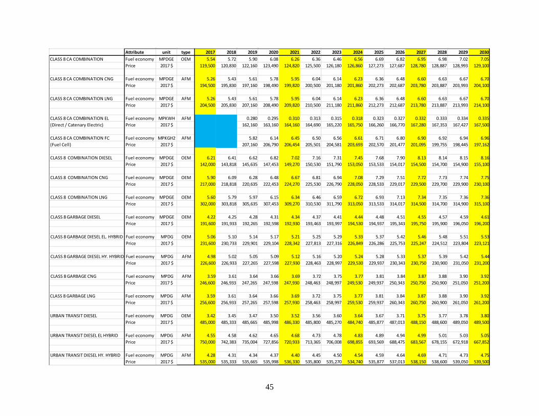
45

Attribute unit type 2017 2018 2019 2020 2021 2022 2023 2024 2025 2026 2027 2028 2029 2030CLASS 8 CA COMBINATION Fuel economy MPDGE OEM 5.54 5.72 5.90 6.08 6.26 6.36 6.46 6.56 6.69 6.82 6.95 6.98 7.02 7.05

Price 2017 $ 119,500 120,830 122,160 123,490 124,820 125,500 126,180 126,860 127,273 127,687 128,780 128,887 128,993 129,100

CLASS 8 CA COMBINATION CNG Fuel economy MPDGE AFM 5.26 5.43 5.61 5.78 5.95 6.04 6.14 6.23 6.36 6.48 6.60 6.63 6.67 6.70Price 2017 $ 194,500 195,830 197,160 198,490 199,820 200,500 201,180 201,860 202,273 202,687 203,780 203,887 203,993 204,100

CLASS 8 CA COMBINATION LNG Fuel economy MPDGE AFM 5.26 5.43 5.61 5.78 5.95 6.04 6.14 6.23 6.36 6.48 6.60 6.63 6.67 6.70Price 2017 $ 204,500 205,830 207,160 208,490 209,820 210,500 211,180 211,860 212,273 212,687 213,780 213,887 213,993 214,100

CLASS 8 CA COMBINATION EL Fuel economy MPKWH AFM 0.280 0.295 0.310 0.313 0.315 0.318 0.323 0.327 0.332 0.333 0.334 0.335(Direct / Catenary Electric) Price 2017 $ 162,160 163,160 164,160 164,690 165,220 165,750 166,260 166,770 167,280 167,353 167,427 167,500

CLASS 8 CA COMBINATION FC Fuel economy MPKGH2 AFM 5.82 6.14 6.45 6.50 6.56 6.61 6.71 6.80 6.90 6.92 6.94 6.96(Fuel Cell) Price 2017 $ 207,160 206,790 206,454 205,501 204,581 203,693 202,570 201,477 201,095 199,755 198,445 197,162

CLASS 8 COMBINATION DIESEL Fuel economy MPDGE OEM 6.21 6.41 6.62 6.82 7.02 7.16 7.31 7.45 7.68 7.90 8.13 8.14 8.15 8.16Price 2017 $ 142,000 143,818 145,635 147,453 149,270 150,530 151,790 153,050 153,533 154,017 154,500 154,700 154,900 155,100

CLASS 8 COMBINATION CNG Fuel economy MPDGE OEM 5.90 6.09 6.28 6.48 6.67 6.81 6.94 7.08 7.29 7.51 7.72 7.73 7.74 7.75Price 2017 $ 217,000 218,818 220,635 222,453 224,270 225,530 226,790 228,050 228,533 229,017 229,500 229,700 229,900 230,100

CLASS 8 COMBINATION LNG Fuel economy MPDGE OEM 5.60 5.79 5.97 6.15 6.34 6.46 6.59 6.72 6.93 7.13 7.34 7.35 7.36 7.36Price 2017 $ 302,000 303,818 305,635 307,453 309,270 310,530 311,790 313,050 313,533 314,017 314,500 314,700 314,900 315,100

CLASS 8 GARBAGE DIESEL Fuel economy MPDGE OEM 4.22 4.25 4.28 4.31 4.34 4.37 4.41 4.44 4.48 4.51 4.55 4.57 4.59 4.61Price 2017 $ 191,600 191,933 192,265 192,598 192,930 193,463 193,997 194,530 194,937 195,343 195,750 195,900 196,050 196,200

CLASS 8 GARBAGE DIESEL EL. HYBRID Fuel economy MPDG OEM 5.06 5.10 5.14 5.17 5.21 5.25 5.29 5.33 5.37 5.42 5.46 5.48 5.51 5.53Price 2017 $ 231,600 230,733 229,901 229,104 228,342 227,813 227,316 226,849 226,286 225,753 225,247 224,512 223,804 223,121

CLASS 8 GARBAGE DIESEL HY. HYBRID Fuel economy MPDG AFM 4.98 5.02 5.05 5.09 5.12 5.16 5.20 5.24 5.28 5.33 5.37 5.39 5.42 5.44Price 2017 $ 226,600 226,933 227,265 227,598 227,930 228,463 228,997 229,530 229,937 230,343 230,750 230,900 231,050 231,200

CLASS 8 GARBAGE CNG Fuel economy MPDG AFM 3.59 3.61 3.64 3.66 3.69 3.72 3.75 3.77 3.81 3.84 3.87 3.88 3.90 3.92Price 2017 $ 246,600 246,933 247,265 247,598 247,930 248,463 248,997 249,530 249,937 250,343 250,750 250,900 251,050 251,200

CLASS 8 GARBAGE LNG Fuel economy MPDG AFM 3.59 3.61 3.64 3.66 3.69 3.72 3.75 3.77 3.81 3.84 3.87 3.88 3.90 3.92Price 2017 $ 256,600 256,933 257,265 257,598 257,930 258,463 258,997 259,530 259,937 260,343 260,750 260,900 261,050 261,200

URBAN TRANSIT DIESEL Fuel economy MPDG OEM 3.42 3.45 3.47 3.50 3.52 3.56 3.60 3.64 3.67 3.71 3.75 3.77 3.78 3.80Price 2017 $ 485,000 485,333 485,665 485,998 486,330 485,800 485,270 484,740 485,877 487,013 488,150 488,600 489,050 489,500

URBAN TRANSIT DIESEL EL HYBRID Fuel economy MPDG AFM 4.55 4.58 4.62 4.65 4.68 4.73 4.78 4.83 4.89 4.94 4.99 5.01 5.03 5.05Price 2017 $ 750,000 742,383 735,004 727,856 720,933 713,365 706,008 698,855 693,569 688,475 683,567 678,155 672,918 667,852

URBAN TRANSIT DIESEL HY. HYBRID Fuel economy MPDG AFM 4.28 4.31 4.34 4.37 4.40 4.45 4.50 4.54 4.59 4.64 4.69 4.71 4.73 4.75Price 2017 $ 535,000 535,333 535,665 535,998 536,330 535,800 535,270 534,740 535,877 537,013 538,150 538,600 539,050 539,500

46

Attribute unit type 2017 2018 2019 2020 2021 2022 2023 2024 2025 2026 2027 2028 2029 2030URBAN TRANSIT CNG Fuel economy MPDG AFM 2.91 2.93 2.95 2.97 2.99 3.02 3.06 3.09 3.12 3.15 3.19 3.20 3.22 3.23

Price 2017 $ 530,000 530,333 530,665 530,998 531,330 530,800 530,270 529,740 530,877 532,013 533,150 533,600 534,050 534,500

URBAN TRANSIT BEV Fuel economy MPKWH OEM 0.250 0.251 0.251 0.252 0.252 0.253 0.253 0.254 0.254 0.255 0.255 0.256 0.256 0.257Price 2017 $ 800,000 794,033 788,191 782,473 776,876 770,535 764,310 758,200 753,867 749,644 745,528 740,830 736,236 731,742

URBAN TRANSIT FCEV Fuel economy MPKGH2 OEM 5.16 5.17 5.18 5.19 5.20 5.21 5.22 5.23 5.24 5.25Price 2017 $ 986,330 975,800 965,470 955,336 947,061 938,974 931,071 922,663 914,432 906,374

SHUTTLE BUS GASOLINE Fuel economy MPGG OEM 6.9 7.09 7.28 7.47 7.66 7.81 7.95 8.10 8.19 8.29 8.38 8.45 8.51 8.58Price 2017 $ 76,400 76,690 76,980 77,270 77,560 77,847 78,133 78,420 78,603 78,787 78,970 79,047 79,123 79,200

SHUTTLE BUS DIESEL Fuel economy MPDG OEM 8.63 8.87 9.11 9.34 9.58 9.85 10.11 10.38 10.53 10.67 10.82 10.90 10.98 11.06Price 2017 $ 84,300 84,590 84,880 85,170 85,460 85,747 86,033 86,320 86,503 86,687 86,870 86,963 87,057 87,150

SHUTTLE BUS E85 Fuel economy MPGE OEM 4.97 5.10 5.24 5.38 5.52 5.62 5.73 5.83 5.90 5.97 6.03 6.08 6.13 6.18Price 2017 $ 76,400 76,690 76,980 77,270 77,560 77,847 78,133 78,420 78,603 78,787 78,970 79,047 79,123 79,200

SHUTTLE BUS CNG Fuel economy MPGGE AFM 6.56 6.74 6.92 7.10 7.28 7.42 7.56 7.70 7.78 7.87 7.96 8.02 8.09 8.15Price 2017 $ 88,900 89,190 89,480 89,770 90,060 90,347 90,633 90,920 91,103 91,287 91,470 91,547 91,623 91,700

SHUTTLE BUS DIESEL HYD. HYBRID Fuel economy MPGP AFM 10.53 10.82 11.11 11.40 11.69 12.01 12.34 12.66 12.84 13.02 13.20 13.30 13.40 13.49Price 2017 $ 108,300 108,590 108,880 109,170 109,460 109,747 110,033 110,320 110,503 110,687 110,870 110,963 111,057 111,150

SHUTTLE BUS BEV Fuel economy MPKWH OEM 1.050 1.061 1.071 1.082 1.093 1.104 1.115 1.126 1.137 1.148 1.160 1.171 1.183 1.195Price 2017 $ 824,500 817,308 810,302 803,479 796,831 789,493 782,320 775,309 770,121 765,085 760,197 754,766 749,475 744,319

SCHOOL BUS GASOLINE Fuel economy MPGG OEM 6.25 6.42 6.60 6.77 6.94 7.05 7.17 7.28 7.39 7.51 7.62 7.63 7.64 7.65Price 2017 $ 89,300 89,588 89,875 90,163 90,450 90,770 91,090 91,410 91,630 91,850 92,070 92,213 92,357 92,500

SCHOOL BUS DIESEL Fuel economy MPDG OEM 7.81 8.87 9.11 9.34 9.58 9.85 10.11 10.38 10.53 10.67 10.82 10.90 10.98 11.06Price 2017 $ 97,300 97,588 97,875 98,163 98,450 98,770 99,090 99,410 99,630 99,850 100,070 100,213 100,357 100,500

SCHOOL BUS BEV Fuel economy MPKWH OEM 0.904 0.913 0.922 0.931 0.941 0.950 0.960 0.969 0.979 0.989 0.999 1.009 1.019 1.029Price 2017 $ 124,300 123,538 122,807 122,106 121,435 120,826 120,244 119,689 119,061 118,458 117,880 117,249 116,641 116,056

SCHOOL BUS CNG Fuel economy MPGGE AFM 5.94 6.10 6.27 6.43 6.59 6.70 6.81 6.92 7.02 7.13 7.24 7.25 7.26 7.27Price 2017 $ 109,300 109,588 109,875 110,163 110,450 110,770 111,090 111,410 111,630 111,850 112,070 112,213 112,357 112,500

SCHOOL BUS LPG Fuel economy MPGP AFM 4.74 4.87 5.00 5.13 5.26 5.35 5.43 5.52 5.60 5.69 5.78 5.78 5.79 5.80Price 2017 $ 107,300 117,588 117,875 118,163 118,450 118,770 119,090 119,410 119,630 119,850 120,070 120,213 120,357 120,500

MOTOR COACH DIESEL Fuel economy MPDG OEM 6.96 7.15 7.34 7.53 7.72 7.87 8.01 8.16 8.26 8.36 8.47 8.49 8.52 8.55Price 2017 $ 350,000 351,284 352,567 353,851 355,134 356,102 357,069 358,037 358,770 359,502 360,235 360,323 360,412 360,500

MOTOR COACH CNG Fuel economy MPDGE OEM 5.91 6.07 6.24 6.40 6.56 6.69 6.81 6.94 7.02 7.11 7.20 7.22 7.24 7.27Price 2017 $ 385,000 386,284 387,567 388,851 390,134 391,102 392,069 393,037 393,770 394,502 395,235 395,323 395,412 395,500

47

LIST OF ACRONYMS A Area

AMT Automated manual transmission

APU Auxiliary power unit

ATI Automatic tire inflation

CAFE Corporate average fuel economy

CARB California Air Resources Board

Cd Coefficient of drag

Energy Commission

California Energy Commission

CNG Compressed natural gas

CO2 Carbon dioxide, a greenhouse gas

DOE United States Department of Energy

E85 A blend of 15 percent gasoline and 85 percent ethanol used to fuel dedicated ethanol powered vehicles and flex-fuel vehicles

EGR Exhaust gas recirculation

U.S. EPA United States Environmental Protection Agency

EU European Union

GHG Greenhouse gas

GVW Gross vehicle weight

GVWR Gross vehicle weight rating

HDS H-D Systems

HHDT Heavy-heavy duty truck

HVAC Heating, ventilation, and air conditioning

IEPR Integrated Energy Policy Report

kg Kilogram

kW Kilowatt, a unit of power

kWh Kilowatt-hour, a unit of energy

LHD Light-heavy duty (truck)

LNG Liquefied natural gas

MDT Medium-duty truck

48

MHD Medium-heavy-duty (truck)

MPDG Miles per diesel gallon

MPDGE Miles per diesel gallon equivalent

MPEG Miles per E85 gallon

MPG Miles per gallon

MPGG Miles per gasoline gallon

MPGGE Miles per gasoline gallon equivalent

MPH Miles per hour

MPKGH2 Miles per kilogram of hydrogen

MPKWH Miles per kilowatt-hour

MPGP Miles per gallon of propane

NHTSA National Highway Traffic Safety Administration

NOX Nitrogen oxide

OEM Original equipment manufacturer

PCCI Premixed charge compression ignition

PM Particulate matter

RIA Regulatory Impact Assessment

SCR Selective catalytic reformer

SwRI Southwest Research Institute

TIUS Truck Inventory and Use Survey

TPM Tire-pressure monitoring

V10 Internal combustion engine with 10 cylinders

V8 Internal combustion engine with 8 cylinders

VIUS Vehicle Inventory and Use Survey

WBS Wide-base singles

WHR Waste heat recovery

49

ATTACHMENT I: H-D Systems (EEA) Report to Department Of Energy on Heavy-Duty Truck Fuel Economy

0

TECHNOLOGICAL POTENTIAL TO REDUCE

HEAVY-DUTY TRUCK FUEL CONSUMPTION TO 2025

REVISED FINAL REPORT

PREPARED BY:

H-D SYTEMS WASHINGTON DC 20016

DECEMBER, 2011

PREPARED FOR:

U. S. DEPARTMENT OF ENERGY

UNDER SUBCONTRACT NO.4000106324 UT-BATELLE LLC

OAK RIDGE NATIONAL LABORATORY

0

I-1

TABLE OF CONTENTS

1. INTRODUCTION I-3 2. BASELINE DATA ON TRUCK CHARACTERISTICS AND OPERATIONS 2.1 OVEVIEW I-7

2.2 HEAVY-HEAVY DUTY TRUCK SEGMENT I-9

2.3 LIGHT HEAVY AND MEDIUM HEAVY SEGMENTS B-14

2.4 ENERGY CONSUMPTION ALLOCATION B-18

2.5 REGULATORY CYCLES B-22

3. ENGINE AND DRIVELINE TECHNOLOGY 3.1 BASELINE B-25

3.2 ENGINE IMPROVEMENT TARGETS

AND ACTUAL POTENTIAL B-28

3.3 COMBUSTION IMPROVEMENTS B-31

3.4 WASTE HEAT RECOVERY B-35

3.5 FRICTION LOSS B-37

3.6 ACCESSORY POWER B-39

3.7 TRANSMISSION IMPROVEMENTS B-40

3.8 HYBRID DRIVETRAINS B-42

3.9 SUMMARY B-45

4. AERODYNAMIC DRAG, ROLLING RESISTANCE AND WEIGHT REDUCTION 4.1 AERODYNAMIC DRAG REDUCTION B-47

4.2 ROLLING RESISTANCE REDUCTION B-63

4.3 WEIGHT REDUCTION B-66

I-2

5. FUEL SAVINGS FROM OPERATIONAL IMPROVEMENTS 5.1 OVERVIEW B-70

5.2 SUMMARY OF POTENTIAL SAVINGS B-70

5.3 IDLE REDUCTION B-73

6. FUEL ECONOMY POTENTIAL AND COST EFFECTIVENESS ANALYSIS 6.1 OVERVIEW B-76

6.2 NEW TRUCK SALES ALLOCATION BY CLASS

AND APPLICATION B-76

6.3 EVALUATION OF COST EFFECTIVENESS B-78

6.4 HEAVY-HEAVY TRUCK TECHNOLOGY POTENTIAL B-79

6.5 MEDIUM DUTY TRUCK TECHNOLOGY POTENTIAL B-85

6.6 ABILITY TO MEET THE 2014/2017 STANDARDS B-88

6.6 SUMMARY AND CONCLUSIONS B-90

APPENDIX A: DETAILEDLISTING OF TECHNOLOGY IMPROVEMENT POTENTIAL BY PAYBACK PERIOD B-92

I-3

1 INTRODUCTION

While there has been considerable attention paid to the costs and benefits of reducing fuel

consumption and greenhouse gases from light-duty vehicles, heavy-duty commercial

vehicles have received much less attention in spite of the fact that total fuel consumption

is a significant and growing part of total transportation related fuel consumption. Some of

this lack of attention is due to the widespread belief that trucking is an efficient market

for fuel economy technology since fuel cost is a significant component of total cost of

truck operation, and the commercial nature of the operation suggests that market

inefficiencies will be resolved. However, discussions with truck fleet operators and truck

manufacturers show that customers are unwilling to pay for technology that cannot

demonstrate simple payback from fuel savings in about 3 years or less, which implies a

steep discount on the value of lifetime fuel savings. This is partly due to the fact that new

trucks are intensively used for the first 4 to 5 years of operation and then sold to second

owners who use them much less intensively. Hence, the first owner usually expects to

recapture the value of additional technology investment within the ownership period

rather than expect some payback in the resale market. This report examines available

technology to improve truck fuel efficiency and estimates their cost and benefit to

develop a supply curve of fuel efficiency. The outcomes from different assumptions on

the payback in terms of fuel savings allow a detailed computation of fuel savings and the

cost of GHG reduction from the commercial truck sector.

Section 2 provides a summary of the characteristics of the existing fleet of heavy trucks,

sub-divided into three classes based on the gross vehicle weight, termed light-heavy,

medium-heavy and heavy-heavy. The data shows the use, annual mileage and fuel

economy of each of these sub-classes and this type of data is used to gauge the

applicability and benefit of different technologies to each sub-class. The data is from the

2002 VIUS which is relatively old but is unfortunately the only source of comprehensive

data on truck use and real world fuel economy at the disaggregate level desired for this

I-4

analysis. In addition, section 2 discusses the typical drive cycles over which fuel

consumption should be evaluated. Trucks are used in a variety of applications ranging

from long haul to vocational use. The lack of a fixed reference drive cycle by application

is a major drawback in the analysis of fuel economy potential and this section makes a

preliminary attempt to define specific drive cycles and the attendant energy losses for a

number of different uses. These cycles and energy loss estimates form the basis for the

technology benefit estimates over different applications. Since the completion of the draft

of this report, the EPA and DOT have issued HDT fuel economy and GHG standards for

2014 and 2017, and have specified drive cycles for reference. The new drive cycles are

compared to our findings in this report.

Section 3 provides a discussion of the available drive-train technology to improve fuel

economy and most of this data was obtained from interviews of the staff of different

heavy-duty engine manufacturers. The DOE’s 21st Century Truck Program has sponsored

a series of conferences on engine efficiency to assess the goal of attaining 50 percent

thermal efficiency in the near term and 55 percent efficiency in the longer term for the

diesel engine. Technologies identified to meet these goals were assessed for their

potential to meet the goals at reasonable cost, and be brought to market in the time frame

of interest. Based on engine manufacturer inputs, technologies were classified by cost and

potential time frame of introduction.

Section 4 provides an analysis of technologies affecting aerodynamic drag, rolling

resistance and weight reduction, i.e., body technologies. Many of these technologies have

been available in the aftermarket for a long time but most have yet to attain significant

market penetration. Our analysis focuses on the actual as opposed to claimed benefits and

also examines potential negative attributes that may have contributed to the limited

market penetration to date. In addition, our analysis focuses on the fact that many

technologies’ benefits are dependent on the baseline; for example, the benefits of many

drag reducing technologies depends on the aerodynamic characteristics of the base truck

and technology benefits cannot be treated as additive. This analysis creates a framework

for examining marginal benefits based on the drag coefficient of current trucks versus the

drag coefficient thought to be ultimately attainable.

I-5

Unlike the light-duty sector, fuel savings are also available from operational

enhancements that range from reducing idle time to improved maintenance and driving

practices. Operational strategies are not a focus of this effort but are summarized since

many reports on truck fuel economy add these benefits to those attained by technology

improvements, Data on these operational enhancements were largely derived from

existing studies conducted by regulatory agencies such as the EPA, and the benefits and

costs of these operational improvements are also included in section 5. One improvement

is associated with idle reduction devices that fall between a pure vehicle technology

enhancement and an operational enhancement, since the engine is often used to provide

HVAC services for sleeper cabs overnight. This technology is considered in some detail

in this report.

Section 6 documents the construction of the supply curves and the cost-benefit of

technology in broad categories. The supply curves are developed by vehicle class, range

of operation and body style for a total of 14 different truck sub-classes The analysis

provides some insight into the future potential for fuel economy improvements under a

free market and GHG based intervention scenario. One of the interesting findings of this

analysis is that the potential maximum technology benefits in reducing fuel consumption

are similar across most vehicle classes and use types but have very different cost and

payback implications. The revised report also examines compliance with the new fuel

economy standards and the expectation for real world fuel economy.

I-6

I-7

2 BASELINE DATA ON TRUCK CHARACTERISTICS AND OPERATIONS

2.1 OVERVIEW The objective of this study is to develop estimates of the costs and benefits of a variety of

fuel economy improvement options for the heavy-duty trucking sector in order to create a

supply curve of fuel efficiency. This section provides an outline of the data that are used

in the construction of this curve. This study considers technology-based fuel economy

improvements as well as improvements in trucking operational efficiencies. The

functional fleet-wide impact of the fuel economy improvement available from some of

the technology options, and all of the operational options, are a function of both the per

vehicle fuel economy potential of the option as well the operational characteristics of the

fleet – that is, the portion of the fleet for which the option is applicable. This section

presents data that are relevant for the entire fleet, and also documents the operational

characteristics that are relevant for particular fuel efficiency improvements applicable to

a sub-set of the trucking population.

Data for this study about the composition of the heavy-duty trucking vehicle fleet, and

operational characteristics of vehicle use are drawn from the VIUS. The VIUS was

conducted every five years from 1967 through 2002 (but suspended since). The VIUS

data is from a survey conducted by the US Census Bureau that includes data on the

physical and operating characteristics of the US truck population. The survey, the most

recent version of which was collected in 2002/3, includes 98,682 observations with 453

variables on each truck.

The Motor Fuel Consumption model (MFCM) was used to estimate future fuel use and

GHG emissions. The MFCM provides detailed projections of fuel demand by fuel type

and vehicle type, given detailed inputs on the fleet characteristics. In this sense, the

MFCM is an accounting model and has no built-in econometric framework, so that its

I-8

projections are directly connected to inputs with no intermediate processing involving

assumptions on consumer behavior. This simplicity has been useful for examining the

potential impact of changes in vehicle fleet or fuel characteristics. Since the MFCM

outputs are so input driven, the inputs have been periodically revised. DOE has used the

MFCM since the late 1970’s to project on-highway fuel demand.

In this analysis, the heavy-duty truck segment is broken into three sub-categories – Light

Heavy-Duty Trucks (LHDT), Medium Heavy-Duty Trucks (MHDT), and Heavy Heavy-

Duty Trucks (HHDT) – in order to properly represent the technological and operational

differences between the vehicles in each sub-category. LHDT, mostly large pickups and

large cargo vans, share many components with vehicles in the light-duty vehicle sector

and for this analysis include all vehicles in GVW classes 3, 4 and 5. These vehicles are

generally operated about 27,000 + 3000 miles per year, and a substantial fraction of the

fleet is powered by gasoline engines (~50% in 2002). MHDT include a broad range of

vehicle types (pickup and delivery, rough duty for construction and mining applications,

municipal waste, fire and emergency, and city buses), the majority of which are used in

local or regional operations. This category included GVW classes 6, 7 and 8A and trucks

in this class are typically used 35,000 + 3000 miles per year, and the fleet is over 90%

diesel. Gasoline engines for this subclass were phased out in the 1990s. HHDT (GVW

class 8B) dominate heavy trucking fuel demand and are comprised mostly of long-haul

tractor trailers (70% of HHDT) along with some construction and mining trucks. The

trucks are used for long haul applications and average 98,000 miles per year. These

trucks have been 100% diesel powered for many decades. Due to the differences in the

technological make up and operational characteristics of each of the heavy-duty trucking

segments, each sub-class is considered separately in this analysis. Data at this level of

aggregation is utilized in this report to estimate the applicability and cost-effectiveness of

different technological options to reduce fuel consumption

The VIUS dataset includes a variable for GVW classification with 15 categories. These

GVW categories were combined to create LHDT, MHDT and HHDT distinctions

according to the following definition: LHDT covers vehicles in the 8,500 to 19,000

pounds GVW range, MHDT covers vehicles in the 19,001 to 50,000 pounds range and

HHDT covers vehicles over 50,000 pounds GVW.

I-9

2.2 HEAVY-HEAVY DUTY TRUCK (HHDT) SEGMENT

HHDT dominate demand for highway diesel fuel. The MFCM projects that HHDT will

account for 67% of total highway diesel demand in 2020. This is a modest decline in

percentage terms from the share in 2007 of 72%; however it represents an absolute

increase of 23%, with annual consumption increasing from 26.6 billion gallons to 32.7

billion gallons, over the period as shown in Figure 2-1.

Figure 2-1: HHDT Diesel Demand

HHDT use is the greatest in the first 5 or 6 years of the vehicle lifetime, with annual

mileage dropping steadily over the life of the vehicle. Figure 2-2 shows the decline in

VMT by vehicle age for HHDT. The consideration of the operational characteristics of

HHDT 5 years old or less is important because it represents the vehicle uses for the first-

owners of HHDT – those that buy from the new vehicle market. Typically, trucks are

used most heavily in their first 3 to 5 years, and are then sold into the secondary market.

Efficiency improvements for new vehicles added to the fleet are chosen based on the

operational characteristics of vehicles less than 5 years old, while efficiency

improvements that are operational or retrofits apply to the entire existing fleet. While

Highway Diesel Demand

0

10

20

30

40

50

60

2007 2008 2009 2010 2011 2012 2013 2014 2015 2016 2017 2018 2019 2020 2021 2022 2023 2024 2025 2026 2027 2028 2029 2030

Year

Bill

ion

Bar

rels

per

yea

r

Total Diesel Demand HHDT Diesel Demand

I-10

figure 2-2 shows that mileage decreases with age, over a third of all HHDTs travel over

75,000miles annually as shown in Figure 2-3.

Figure 2-2: VMT by Vintage

Of all HHDT, 69% are tractors, rather than single unit vehicles. VIUS includes a survey

question that asks respondents what percent of miles are driven with less than truckload

service. This value is useful for calculating the population of vehicles for which fuel

economy, on a per ton-mile basis, could be improved by changing government

regulations limiting trailer length. 16% of miles, on average, are at less than truckload

for tractor-style HHDT, leaving around 58% of total HHDT miles (69% times 84%)

applicable for efficiency improvement from changes to trailer length limits.

Mileage is also characterized within VIUS according to the trip-length category in which

mileage is accumulated. The largest portion of miles for all heavy-duty trucks up to

Class 8A is in trips that are less than 50 miles per trip one-way. The HHDT category has

trip length significantly shifted toward longer distance trips compared to the other heavy-

duty subcategories as indicated in Figure 2-3. Almost 45% of all Class 8B trucks are used

for trips whose length is over 200 miles, and this number is even higher for tractors with

van body trailers. Off-road trip mileage is used to indicate vehicles for which advanced

VMT of Class 8b

y = -29497Ln(x) + 136447R2 = 0.8915

-

20,000

40,000

60,000

80,000

100,000

120,000

140,000

160,000

2002,2003

2001 2000 1999 1998 1997 1996 1995 1994 1993 1992 1991 1990 1989 1988 1987 pre-1987

Vintage

VM

T average

Log. (average)

I-11

tires are not applicable because of the increased risk of tire damage, and for vehicles for

which evolutionary improvements in the front-end aerodynamics are not applicable. Off-

road miles are disproportionately distributed among HHDT – that is, most trucks have

nearly zero off road mileage and the trucks that do make off road trips account for the

majority share of total off-road mileage. The majority of total off-road mileage is

accounted for by approximately the small percentage of HHDT that make a relatively

high proportion of off-road trips – typically construction or mining vehicles.

Figure 2-3: Mileage By Trip Length HHDT

For aerodynamic improvements that are related to the trailer, rather than to the front end

of the vehicle (tractor related), the vehicle population is limited to HHDT that haul a van-

style trailer. Of the entire HHDT fleet, approximately 42% haul a van style trailer while

for younger vehicles (again, 5 years old or less) this figure rises to 63%.

Another opportunity for operational fuel savings is via driver training to educate drivers

on how to optimize vehicle performance to minimize fuel use and costs. Fleet size is

used as a metric of the applicability of this option to improve fuel economy – vehicles in

small fleets are expected to benefit from driver training while drivers in large fleets (>20

tractors) usually already have a driver training program in place. The distribution of

Class 8b

0%

5%

10%

15%

20%

25%

30%

< 50 miles 51-100 miles 101-200 miles 201-500 miles >500 miles off road

Trip Length

Per

cent

age

of T

otal

Mile

age

Class 8b

I-12

HHDT population by fleet size (not including the vehicle surveyed) for both the entire

fleet and for the fleet limited to vehicles 5 years old or less show that (summing the

categories that are >20 tractors in a fleet) driving training can be applicable for 79% of

the existing fleet and 61% of the new vehicle fleet.

Fuel economy by model year shows statistically significant increases over time. As of

2002, the year in which the VIUS data were collected, the average HHDT fuel economy

was 5.86 miles per gallon with newer vehicles showing higher fuel economy. Vehicles 5

years or younger average 5.98 miles per gallon and the newest model year vehicles

(2002/2003 in this survey) averaging almost 6.1mpg. Figure 2-4 shows the trend of fuel

economy against vehicle vintage, and it should be noted that in this case that this is not an

effect of truck age, but due to the fact that truck technology improves over time. The rate

of improvement observed is about 0.5% per year for all Class 8B trucks but increases to

about 0.7% per year for long haul use trucks over the 1987 to 2001 period. Anecdotal

evidence suggests that about 0.4% to 0.45% was due to engine improvements and the

vehicle improvements account for 0.25% to 0.3% per year on the long haul segment.

Trucks used in rough duty applications or short haul appear to have much lower fuel

economy gains of only about 0.25% per year, potentially only from engine

improvements.

The fuel economy changes after 2001 have been measured by DOT in its comparative

evaluation of rail versus truck efficiency, but the data is less reliable than VIUS data due

to the much smaller sample size. The lower figure in Figure 2-4 shows that fuel economy

actually declined from around 5.9 mpg attained in 2000/2001 to about 5.4 mpg in 2002,

which is a decline of about 8.5%, associated with the phase-in of the NOx standard of 4

g.bhp-hr. The incorporation of urea-SCR systems in 2010 appear to have more than

reversed the trend and the data shows newest trucks attaining 6.6 mpg. However, the data

appears to exaggerate the effects of the NOX standards, and truck manufacturers suggest

that the decline from the 4 and 2 g/bhp-hr standards were on the order of 5% which has

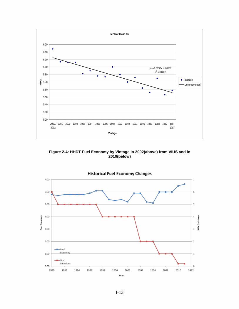
I-13

Figure 2-4: HHDT Fuel Economy by Vintage in 2002(above) from VIUS and in 2010(below)

MPG of Class 8b

y = -0.0292x + 6.0537R2 = 0.8083

5.20

5.30

5.40

5.50

5.60

5.70

5.80

5.90

6.00

6.10

6.20

2002,2003

2001 2000 1999 1998 1997 1996 1995 1994 1993 1992 1991 1990 1989 1988 1987 pre-1987

Vintage

MP

G average

Linear (average)

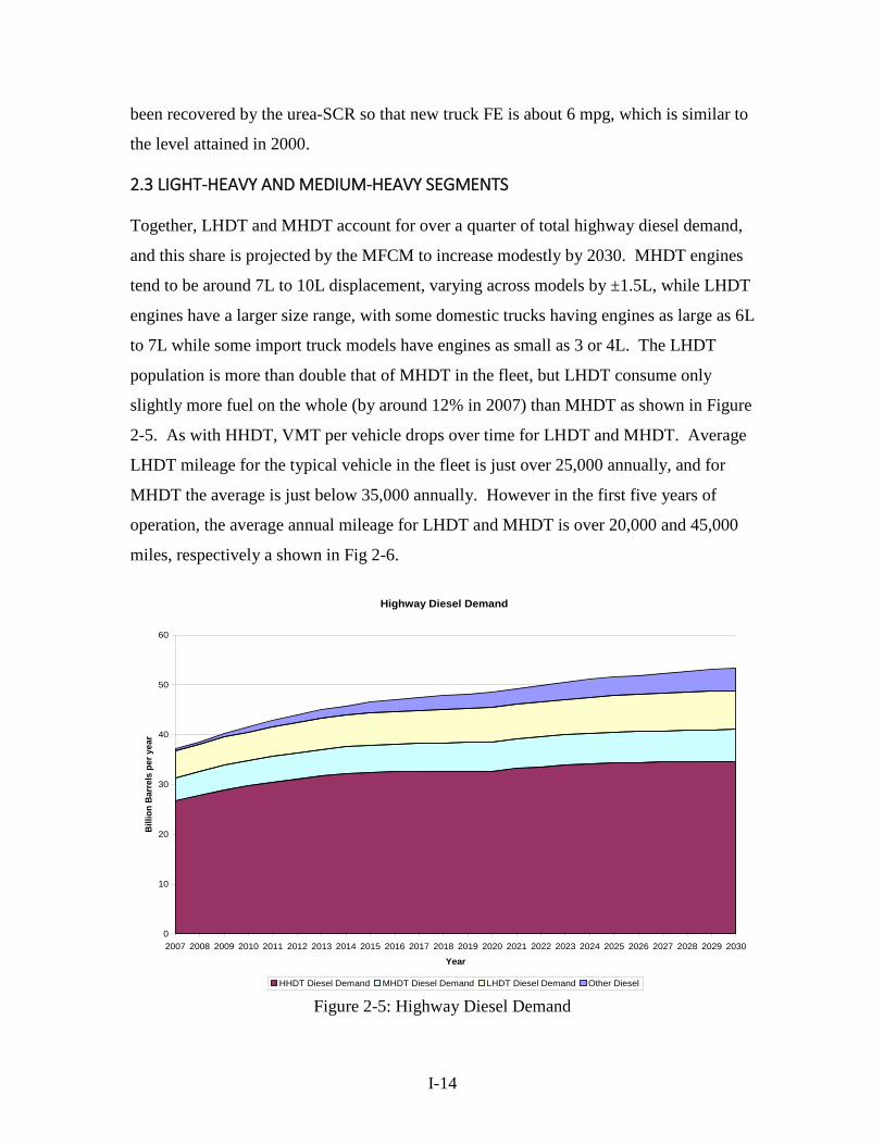
I-14

been recovered by the urea-SCR so that new truck FE is about 6 mpg, which is similar to

the level attained in 2000.

2.3 LIGHT-HEAVY AND MEDIUM-HEAVY SEGMENTS Together, LHDT and MHDT account for over a quarter of total highway diesel demand,

and this share is projected by the MFCM to increase modestly by 2030. MHDT engines

tend to be around 7L to 10L displacement, varying across models by ±1.5L, while LHDT

engines have a larger size range, with some domestic trucks having engines as large as 6L

to 7L while some import truck models have engines as small as 3 or 4L. The LHDT

population is more than double that of MHDT in the fleet, but LHDT consume only

slightly more fuel on the whole (by around 12% in 2007) than MHDT as shown in Figure

2-5. As with HHDT, VMT per vehicle drops over time for LHDT and MHDT. Average

LHDT mileage for the typical vehicle in the fleet is just over 25,000 annually, and for

MHDT the average is just below 35,000 annually. However in the first five years of

operation, the average annual mileage for LHDT and MHDT is over 20,000 and 45,000

miles, respectively a shown in Fig 2-6.

Figure 2-5: Highway Diesel Demand

Highway Diesel Demand

0

10

20

30

40

50

60

2007 2008 2009 2010 2011 2012 2013 2014 2015 2016 2017 2018 2019 2020 2021 2022 2023 2024 2025 2026 2027 2028 2029 2030

Year

Billi

on B

arre

ls p

er y

ear

HHDT Diesel Demand MHDT Diesel Demand LHDT Diesel Demand Other Diesel

I-15

Figure 2-6 Annual Miles by Vintage and Class

. The distribution of mileage among the LHDT and MHDT subcategories is also much less

variable than for the HHDT subcategory. Just over 10% of LHDT travel more than

30,000 miles annually, and fewer than 5% travel more than 50,000 miles annually.

Similarly, just over 6% of MHDT travel more than 50,000 miles on an annual basis. On

the other hand, over a third of MHDT travel less than 5,000 miles on an annual basis and

over 70% of both LHDT and MHDT travel less than 20,000 miles annually, as shown in

figure 2-7 below

VMT of Class 3-5 and 6-8a

y = -3038.9Ln(x) + 28062R2 = 0.2329

y = -6591.7Ln(x) + 41980R2 = 0.5826

-

5,000

10,000

15,000

20,000

25,000

30,000

35,000

40,000

45,000

2002,2003

2001 2000 1999 1998 1997 1996 1995 1994 1993 1992 1991 1990 1989 1988 1987 pre-1987

Vintage

VM

T

short (3-5)

short (6-8a)

Log. (short (3-5))

Log. (short (6-8a))

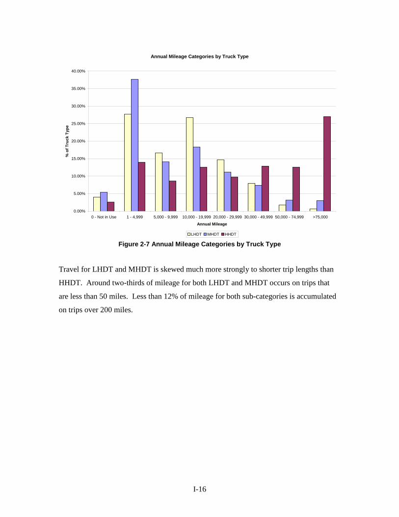
I-16

Figure 2-7 Annual Mileage Categories by Truck Type

Travel for LHDT and MHDT is skewed much more strongly to shorter trip lengths than

HHDT. Around two-thirds of mileage for both LHDT and MHDT occurs on trips that

are less than 50 miles. Less than 12% of mileage for both sub-categories is accumulated

on trips over 200 miles.

Annual Mileage Categories by Truck Type

0.00%

5.00%

10.00%

15.00%

20.00%

25.00%

30.00%

35.00%

40.00%

0 - Not in Use 1 - 4,999 5,000 - 9,999 10,000 - 19,999 20,000 - 29,999 30,000 - 49,999 50,000 - 74,999 >75,000

Annual Mileage

% o

f Tru

ck T

ype

LHDT MHDT HHDT

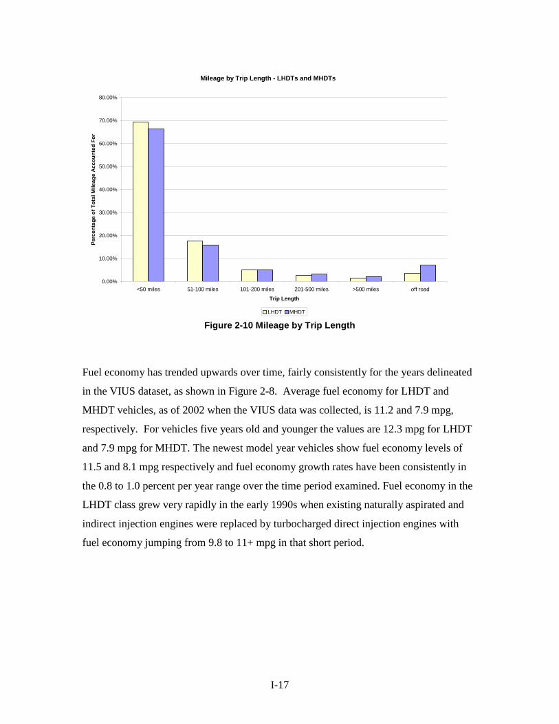
I-17

Figure 2-10 Mileage by Trip Length

Fuel economy has trended upwards over time, fairly consistently for the years delineated

in the VIUS dataset, as shown in Figure 2-8. Average fuel economy for LHDT and

MHDT vehicles, as of 2002 when the VIUS data was collected, is 11.2 and 7.9 mpg,

respectively. For vehicles five years old and younger the values are 12.3 mpg for LHDT

and 7.9 mpg for MHDT. The newest model year vehicles show fuel economy levels of

11.5 and 8.1 mpg respectively and fuel economy growth rates have been consistently in

the 0.8 to 1.0 percent per year range over the time period examined. Fuel economy in the

LHDT class grew very rapidly in the early 1990s when existing naturally aspirated and

indirect injection engines were replaced by turbocharged direct injection engines with

fuel economy jumping from 9.8 to 11+ mpg in that short period.

Mileage by Trip Length - LHDTs and MHDTs

0.00%

10.00%

20.00%

30.00%

40.00%

50.00%

60.00%

70.00%

80.00%

<50 miles 51-100 miles 101-200 miles 201-500 miles >500 miles off road

Trip Length

Perc

enta

ge o

f Tot

al M

ileag

e A

ccou

nted

For

LHDT MHDT

I-18

Figure 2-11 LHDT and MHDT Fuel Economy by Vintage

2.4 ENERGY CONSUMPTION ALLOCATION

The energy use by trucks has not been intensively studied as for light vehicles because

there is no specific test cycle or driving cycle that is used as a reference. Since long haul

trucks accumulate most of their mileage on the highway, some analyses have used a 65

mph constant speed case as a reference condition to allocate energy use to the different

components, using analysis based on the first law of thermodynamics. In these analyses,

the conversion of fuel energy by the diesel engine to shaft work is always the biggest user

since the engine efficiency during driving is about 40%, implying that 60% of the energy

is lost in this step. Other components of loss are much smaller, but this is misleading

since it is the efficiency of the diesel engine which is approximately constant, not the

absolute energy loss in fuel conversion, and a 10% reduction in shaft work results in a

10% reduction in fuel use. Figure 2-12 below is derived from DOE’s 21st Century Truck

Program for a constant speed 65 mph case.

MPG of Class 3-5 Diesel and 6-8a

y = -0.196x + 13.334R2 = 0.6827

y = -0.0714x + 8.5624R2 = 0.7254

0

2

4

6

8

10

12

14

2002,2003

2001 2000 1999 1998 1997 1996 1995 1994 1993 1992 1991 1990 1989 1988 1987 pre-1987

Vintage

MP

G

average (3-5)average (6-8a)Linear (average (3-5))Linear (average (6-8a))

I-19

Figure 2-11: Allocation of Class 8B Truck Fuel Consumption at 65 mph.

In this case, base case engine output is 160 kW, with aerodynamic losses accounting for

85 kW or 53% of shaft work, tire rolling resistance for 51 kW or 32% of shaft work and

the drive train friction loss and accessory drives accounting for 5.6% and 9.4% of shaft

work. However, the constant speed condition is very unrealistic since rolling hills, road

curves and traffic generally result in continuous speed and load variations as well as

losses to the brakes. Steeper grades on mountainous geography have a very large effect

but also affect the speed that trucks can maintain. Cummins provided a breakdown of

shaft work on a “typical” long haul cycle in the Mid-west (i.e., modest road congestion

and terrain effects) as shown in Figure 2-13, and this cycle uses 173 hp (129 kW) at an

approximate average speed of 48 mph for class 8B truck.

I-20

Figure 2-13: Power Demand for Typical Cycles on Heavy- Duty Trucks

The Cummins cycle shows a loss of 13 to 14% of shaft work to the brakes, with

aerodynamic drag accounting for about 40% of shaft work, and rolling resistance

accounting for about 37% of shaft work. Accessory drives account for 5% while driveline

loss accounts for the remaining 4%. In this case, energy use is about 2.69 kWhr per mile

as compared to 2.46 kWhr per mile in the constant speed 65mph case, which is 9%

higher. In addition, idle fuel consumption is not accounted for in shaft work related

analyses and is around 4 to 7 percent of total fuel for long haul trucks based on expert

opinion (no hard data is available to estimate the idle fraction in real life). In vehicles

with sleeper cabs, idle fuel consumption may be much higher if the engine runs all night

to provide HVAC power for the cab. The Cummins cycle may underestimate actual brake

losses since traffic congestion is much higher in the East and West Coast, while the

topography in the mountain states may also result in larger braking energy loss.

I-21

In addition, fuel use at idle is not directly accounted for in analysis of tractive energy use

and idle fuel use is not well documented or known. In some analyses of savings

associated with idle reduction devices, EPA assumed that trucks idle 8 hours a day, 300

days a year for a total of 2400 hours per year. With fuel consumption at idle estimated at

0.8 to 0.9 gallons per hour, annual fuel use is about 2000 gallons which is 8 to 10 percent

of total fuel use. These numbers appear very high from anecdotal information, and may

be applicable only to the subset of trucks with sleeper cabs. In other HHDT applications,

anecdotal information suggests that fuel use at idle may be only 2 to 4 percent of

consumption, so that on aggregate, it is 4 to 6 percent of total fuel use as sleeper cab

equipped vehicles account for about a third of all Class 8B trucks. Based on these

estimates, we constructed energy and fuel use allocations as follows, to the nearest half

percent

Traction Energy Fuel Use

Idle 0 5 + 0.5

Inertia (lost to brakes) 13 + 1 12.5 + 1

Aerodynamics 40 + 2 38 + 2

Tire Rolling Resistance 37 + 2 35 + 2

Accessory Drives 6 + 1 5.5 + 0.5

Drive-train Loss 4 + 1 4 + 0.5

These allocations are utilized in the following sections to estimate Class 8B long haul

truck related technology benefits. Allocations for other classes of trucks are more

difficult because of the large variances in duty cycles. MHDT are used in suburban and

short haul routes (less than 200 miles radius) for freight delivery, while many are used in

urban pick-up and delivery, or by utilities (gas, electric, water, garbage). The “refuse”

cycle shown in Figure 2-13 above shows average power of 95 hp (71kW) with 38% in

inertia loss, 19% in accessory loads, 27% in driveline losses, 9% in tire loss and only 7%

in aerodynamic drag loss. In general, MHDT have higher drive-train loss due to the

relatively widespread use of automatic transmissions.

I-22

The Federal Test procedure for light duty vehicles has two drive cycles, one at 19 mph

(city) and one at 48 mph (highway) with a weighted composite representing typical

urban/suburban driving. The energy use for that cycle has been solved by numerical

integration as a function of the drag to weight ratio and rolling resistance to weight ratio,

and based on that solution we have derived the following values for fuel use fractions

shown in Table 2-1:

Line Haul

(Manual

Trans)

Regional

Haul (Man.

Trans.)

Urban/

Suburb.

(Auto

Trans)

Refuse/ Bus

(Auto Trans)

Idle/ Decel. 5 + 0.5 7 + 0.5 8 + 0.5 15 + 1

Inertia (lost to brakes) 12.5 + 1 31.5 + 2 26.5 + 2 32 + 2

Aerodynamics 38 + 2 25 + 2 20 + 2 6 + 0.5

Tire Rolling Resistance 35 + 2 25 + 2 21.5 + 2 8 + 0.5

Accessory Drives 5.5 + 0.5 7 + 0.5 9 + 0.5 16 + 1

Drive-train Loss 4 + 0.5 5.5 + 1 15 + 1 23 + 1

2.5 REGULATORY CYCLES

The new regulations for HDT fuel economy announced in August 2011 incorporate drive

cycles for fuel economy evaluation. However, the cycles incorporated appear to be

relatively simplistic and quite general. The regulation requires separate testing of engines

on the standard FTP and a simulation model approach for the entire vehicle.

The engine FTP cycle consists of 2 low speed cycles, the New York and Los Angeles

non-freeway cycles, and one medium speed cycle called the Los Angeles freeway cycle.

The cycle results are weighted to produce a near equal mileage on freeway and non-

freeway operation which EPA recognized as not being representative of either

I-23

“vocational” trucks or long haul trucks. Instead, three new cycles were selected. One was

a new Transient cycle with an average speed of 15.3 mph and a distance of 2.84 miles,

and includes almost 17% of the time at idle. The other 2 cycles are simply two constant

speed modes at 55 mph and 65 mph, with no gradients or transients. The same three

modes are applied to all trucks with different weightings. For sleeper cab equipped long

haul trucks, the 65 mph constant speed mode is VMT weighted at 86% of operation while

the 55 mph mode is weighted at 9%, with only the remaining 5% weighing for the

transient cycle. For day cab equipped tractors, the weightings are 64%, 17% and 19%

respectively. Even for vocational vehicles, the EPA assumes 37% of the VMT at 65 mph

and 21% at 55 mph, with only 42% on the transient mode.

The analysis presented in Sections 2.3 and 2.4 show that the EPA assumptions of

constant speed cruise at 55/65 mph are quite unrealistic, and essentially remove the role

of inertia, while over-emphasizing the role of aerodynamic drag and tire rolling

resistance. In addition, it is not clear if engine technology improvements will be fairly

represented in the selected cycles as the benefit of some technologies such as turbo-

compounding are better at constant high speed high load points on the engine map, and

would provide a larger benefit on the test than in the real world.

I-24

I-25

3 ENGINE AND DRIVELINE TECHNOLOGY

3.1 BASELINE

Engines used in most heavy duty trucks over 10,000 pounds. GVW are powered by diesel

engines, with all gasoline engines have essentially been phased out and only a few

gasoline engines sold in the 10K to 14K GVW class trucks. Diesel engines have been

historically classified as light heavy, medium heavy and heavy-heavy by the EPA with

different durability requirements. In the light heavy class, engines were typically in the

6L to 9L displacement range; in the medium heavy class, the were in the 7L to 11L range

and heavy-heavy trucks used engines over 11L. With the advent of common rail fuel

injection systems and high pressure turbo-charging, engine specific output has increased

significantly and the lines of distinction between classes are not as well defined.

In the light heavy class, the Cummins B-series 6.7L, the Navistar 6.4L and the GM 6.6L

engines account for the vast majority of engines sold, with the Cummins 6 cylinder

engine sold on Dodge trucks, the Navistar V8 engine on Ford trucks, and the GM V8

engine on Chevy/GMC trucks. In the medium duty sector, the Navistar DT 466 engine,

the Cummins C series 8.3L engine and the Detroit Series 50 (now replaced by a

Mercedes engine) are the most popular models. In the heavy-heavy category, the

Cummins M series engine and the N series engine, the Caterpillar C13 and the DDC

series 60 engine were the most popular. These engines have been updated or replaced for

2010 by the ISX13 and 15 engines from Cummins and the Mercedes 13L and 15L

engines, while Caterpillar’s on-highway engines have been discontinued and replaced by

the “Maxxforce” 11 and 13 engines. The Mercedes 15L engines are the first turbo-

compound engines sold in North America. In addition, many light heavy engines are used

in medium duty applications, while the medium duty engines are now used in many of

the lighter weight heavy-heavy applications.

In class 8 trucks, the vast majority (about 75%) use the 10 speed manual transmission,

while only about 8% (mostly vocational trucks) use automatic transmissions. The

I-26

remainder used manual transmissions with higher number of speeds, typically 12 or 16.

This is consistent with the information in the VIUS which shows the heavy-heavy

segment having 92.3% manual transmissions, 6 percent automatics and 1.7% automated

manual transmissions. In medium duty trucks, the numbers are almost reversed with

about 75 percent using six-speed automatic transmissions and 5 to 8 percent using the

automated manual transmission (AMT). The VUIS data shows automatic penetration at

78.2% but has automated manual transmissions at only 0.7%, but AMT models have been

newly introduced since 2002 and the information from manufacturers seems defensible.

The remainder use 6 or 8 speed manual transmissions. At the light heavy end, almost 70

percent use automatic transmissions which were largely 4 –speed units in 2008 but are

now transitioning to 6-speed units. The remaining 30 percent use 5 or 6 speed manual

transmissions, and these numbers are confirmed in the VUIS data.

The efficiency of diesel engines over time has improved at slightly under 0.4% per year

over the 1975 to 2003 period but has since decreased due to the imposition of strict Nox

emission standards in 2004 of 2.5 g/bhp-hr, followed by the PM standards and the further

tightening of the NOx standards in 2007 and 2010.

As shown in the figure 3-1 above, the peak efficiency point (right scale) of advanced

heavy-duty diesels reached a maximum of about 44% but then declined to about 40%. In

2010, most heavy-heavy duty diesels will use exhaust after-treatment to control NOx that

will allow engine-out emissions to increase relative to the 2007-2009 engines with

efficiency increasing to 42%. The figure above also shows Volvo’s hypothetical

projection of efficiency at constant NOx emissions standards suggesting that fuel

consumption has increased by 11% relative to this hypothetical level, but other

manufacturers suggest that the loss may be only 5 to 6 percent, suggesting a peak

efficiency of close to 45% at engine out NOx levels of 6g/ bhp-hr, a standard that has

been in force since 1990. The historical rate of improvement estimated from the 38%

efficiency level in 1980 to 44% in 2000 suggests engine thermal efficiency improvements

on the order of 0.3% per year or a fuel economy improvement of 0.73% per year.

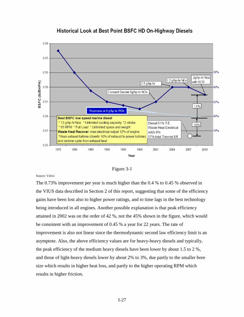
I-27

Figure 3-1 Source: Volvo

The 0.73% improvement per year is much higher than the 0.4 % to 0.45 % observed in

the VIUS data described in Section 2 of this report, suggesting that some of the efficiency

gains have been lost also to higher power ratings, and to time lags in the best technology

being introduced in all engines. Another possible explanation is that peak efficiency

attained in 2002 was on the order of 42 %, not the 45% shown in the figure, which would

be consistent with an improvement of 0.45 % a year for 22 years. The rate of

improvement is also not linear since the thermodynamic second law efficiency limit is an

asymptote. Also, the above efficiency values are for heavy-heavy diesels and typically,

the peak efficiency of the medium heavy diesels have been lower by about 1.5 to 2 %,

and those of light-heavy diesels lower by about 2% to 3%, due partly to the smaller bore

size which results in higher heat loss, and partly to the higher operating RPM which

results in higher friction.

I-28

3.2 ENGINE IMPROVEMENT TARGETS AND ACTUAL POTENTIAL

Cummins provided a detailed map of energy flows for a recent model engine with a brake

efficiency of 42%, as shown in Figure 3-2. Indicated efficiency of 50% is the current

combustion duration limited diesel cycle efficiency, but with high EGR flow, there is

more heat rejection to the coolant and EGR coolers than to exhaust. Heat rejection to

exhaust has decreased from about 30 percent before the use of EGR (pre-2004) to 26

percent now, which has ramifications for the efficiency of heat recovery from turbo-

compounding. Caterpillar data for a C15 engine with 42 percent efficiency shows exhaust

gas heat rejection at 22 percent, but also shows heat loss from low pressure EGR (post

Turbo) to be 5% for a total of 27% heat available after the turbo- charger. The heat loss

values in figure 3-3 form the basis for Cummins’ analysis of improving the brake

efficiency to 52.5% in the future.

Figure 3-2: Distribution of Energy Losses in Current Engine

I-29

Figure 3-3 shows the energy flows modeled by Cummins to achieve the 52.5% efficiency

target. This would require increasing indicated efficiency to 58%, while significantly

reducing gas exchange losses indicating a fuel economy (FE) benefit of 25% (52.5/42-1).

This would be the benefit for the base engine, and exhaust heat recovery could add

another 6 to 8 percent fuel efficiency with advanced heat recovery systems, leading to a

potential target figure of 31 to 33 percent FE improvement from the engine alone (engine

total efficiency would be around 55%). Of course, the entire benefits of the target may

not be attained in practice. If the historical FE improvement rate of about 0.45 % per year

were to continue to 2030, engines would be 9.5% more fuel efficient by 2030 relative to

2010. Hence, there is a potential margin of 21% to 23% additional FE available from

additional technology to meet the DOE engine efficiency targets. However, most

manufacturers believe that such a large increase will not be possible and reaching 49% to

50% brake efficiency itself will be a major challenge,

Figure 3-3: Estimated Distribution of Energy Loss in Advanced Engine

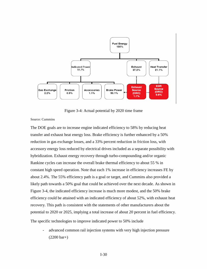
I-30

Figure 3-4: Actual potential by 2020 time frame

Source: Cummins

The DOE goals are to increase engine indicated efficiency to 58% by reducing heat

transfer and exhaust heat energy loss. Brake efficiency is further enhanced by a 50%

reduction in gas exchange losses, and a 33% percent reduction in friction loss, with

accessory energy loss reduced by electrical drives included as a separate possibility with

hybridization. Exhaust energy recovery through turbo-compounding and/or organic

Rankine cycles can increase the overall brake thermal efficiency to about 55 % in

constant high speed operation. Note that each 1% increase in efficiency increases FE by

about 2.4%. The 55% efficiency path is a goal or target, and Cummins also provided a

likely path towards a 50% goal that could be achieved over the next decade. As shown in

Figure 3-4, the indicated efficiency increase is much more modest, and the 50% brake

efficiency could be attained with an indicated efficiency of about 52%, with exhaust heat

recovery. This path is consistent with the statements of other manufacturers about the

potential to 2020 or 2025, implying a total increase of about 20 percent in fuel efficiency.

The specific technologies to improve indicated power to 50% include

- advanced common rail injection systems with very high injection pressure

(2200 bar+)

I-31

- advanced injectors with multiple injections per stroke capability,

- advanced EGR cooling systems,

- closed loop injection control and

- improved air handling with an advanced twin sequential turbochargers or

electrically assisted turbochargers.

3.3 COMBUSTION IMPROVEMENTS

Advanced injection systems and advanced injectors are likely to have a significant

contribution to the overall improvement of efficiency at low engine-out Nox emissions. A

very comprehensive analysis by Bosch shows the dependence of the injection pressure

benefit to be a strong function of engine out Nox level. The 2010 emission standards

require urea-SCR emission control systems that allow engine out Nox levels of 1.0 to 1.1

g/bhp-hr to attain the tailpipe standard of 0.2 g/ bhp-hr implying a catalyst system

efficiency of around 85%. The engine out level translates to about 1.3 to 1.4 g/ kWh in

European terms. As shown in the figure from Bosch below, the benefit of 2400 bar

system over the typical 1800 bar system at this engine output is 3% at the “B50”

operating point corresponding to 50 mph cruise on a highway. Increasing further to 3000

bar could enable an additional 1.5% fuel consumption benefit according to Bosch. These

benefits continue to increase at even lower engine out Nox levels. In this context, engines

operating at lighter average loads (as in trucks used for regional haul at lower speeds)

will see smaller benefits from advanced injection systems.

It should be noted that the new Mercedes engine with turbo-compounding also features a

hydraulically amplified CRS system from Bosch that currently operates at 2300 bar but is

capable of 2500 bar. The next generation 3000 bar pressure systems would likely not

enter the market until late in the next decade, possibly around 2018. Manufacturers

confirm the benefits of increased pressure but suggest that a 2 percent benefit may be

more reasonable as an average. The 2010 Navistar “Maxxforce” engines are being

certified to a 0.5 g/ bhp-hr Nox standard without the use of urea-SCR catalyst systems.

I-32

Figure 3-5: Effect of Common Rail System Pressure on BSFC

They utilize a 2200 bar system, and at this very low engine-out Nox level, the benefit of a

3000 bar system is assessed by Bosch at almost 6%. Manufacturers believe that the

benefits could be around 4% to 5% after subtracting the energy used to increase rail

pressure, but it is not clear if Navistar will continue to use a non-catalytic approach to

meet the 0.2 standard. Moving to the urea- SCR system allows some recovery of

efficiency to a level of 43% to 43.5%, which would improve fuel economy by 2.5% to

3%. However, the systems need to be filled with urea (sometimes referred to diesel

exhaust fluid) which is consumed at a rate equivalent to 2 to 3 percent of fuel

consumption. This level of FE improvement in 2010 has been confirmed by several

engine manufacturers, while Cummins shows an improvement of 4+ % below. However,

the cost of urea is a major concern, and the higher fuel cost of an in-cylinder Nox control

system may be more than offset by the reduction in cost from not having to refill the urea

system. The 2500 bar fuel injection system cost adds about $1500 to retail price over a

2000 bar system, while the 3000 bar system may add $2500 relative to current systems.

I-33

The current urea SCR systems operate at about 80 to 85% cycle efficiency and further

improvement to 90+% is possible over the next five to eight years. This would allow

engine out Nox levels to increase to almost 2 g/bhp-hr at constant tailpipe standards

allowing another 1% efficiency increase or a 2.5% fuel economy increase, corresponding

to a urea-SCR system efficiency increase of about 6 percent in the Figure 3-6. We

anticipate that this improvement will be due to learning and incremental technology

improvements but will not add additional cost to the system.

The sequential twin turbocharger concept has been introduced by several

manufacturers such as Navistar for 2010, and constitutes one form of waste heat

recovery. The twin turbo concept with inter-cooling between stages allows faster throttle

response and more uniform boost capability over the RPM range. The twin turbo concept

allows the engine to be downsized by 10 to 12 percent and still provide adequate low

RPM torque and drivability at low speeds. This level of engine downsizing has occurred

over the last 15 years, with the typical engine size for a 80,000 pounds. GVW vehicle and

a 425 HP rating decreasing from around 15L to 12.5L to 13L. It is not clear if further

downsizing will occur in the market in the near term, but additional downsizing to 11L to

I-34

11.5L is likely in the 2017 to 2025 time frame. DDC reported that improvement in

turbocharger compressor and turbine efficiencies could provide a 1% to 1.5% FE benefit

in the near term. The twin turbo approach has been used with engines certifying at very

low engine-out Nox levels, with the high EGR rate making high boost a requirement to

provide enough air for combustion. We estimate that the twin turbo concept with further

downsizing to provide a 2.5 % to 3 % benefit in fuel economy by 2025. The twin turbo

system adds about $1200 to engine price relative to a single turbo system with the same

HP rating (i.e. a larger displacement engine)

Figure 3-7: Benefits of Closed Loop Combustion Control

Closed loop combustion control has always been seen as a major goal to simultaneously

improve emission and fuel economy performance. The new flexible fuel injection

systems with amplified common rail and advanced injectors capable of multiple

injections can allow PCCI combustion especially at lighter loads up to 10 bar BMEP.

This would be more helpful on medium duty diesel engines, but can provide significant

benefits for the heavy-heavy class as well. Real time combustion control with cylinder

pressure sensing is now possible as sensors are available commercially at reasonable

prices, and cylinder pressure sensing is already being used in some light duty diesels.

I-35

DDC has estimated a thermal efficiency gain of 1 to 2 percent with advanced controllers

with a 37% NOx reduction as shown in Figure 3-7 above, indicating the potential for a

FE gain of up to 5% with reduced emissions. It is possible that the NOx reduction could

be traded for additional efficiency gains. Cylinder pressure sensors for light duty diesel

engines have been commercialized at a cost of about $50 per cylinder. Even if heavy duty

sensors were twice the price, the sensors and wiring should add about $700 to the cost (or

$1100 to RPE) of an in-line 6 cylinder engine.

Gas exchange losses are also helped by the electrically assisted turbo and/or sequential

turbo, but the other technologies to attain this goal include an EGR pump and variable

valve actuation. The EGR pump is a positive contributor to fuel economy only at very

high EGR flow rates that may be required to meet the NOx standards without the use of

urea-SCR. As engines planning to use in-cylinder control technology appear to be

moving to a sequential turbo, low and high pressure loop EGR system, the potential for

the EGR pump appears small and no manufacturer has embraced this technology.

Variable Valve Timing (VVT) can be used to reduce gas exchange loss by increasing

valve overlap to increase internal EGR but this would require a DOHC system, which is

used in some but not all heavy-duty engines. In addition, it can be used to increase

exhaust temperature if needed. Such a system could increase FE by 0.5% to 1.0%, but

performance data on prototype systems have not been released publicly. The timing could

be changed using hydraulic cam phasers similar to those that have been employed in light

duty SI engines. Variable valve actuation is expensive for HHDT engines and has a

payback of about 3 to 4 years, with a cost of about $800.

3.4 WASTE HEAT RECOVERY

Waste heat recovery is a major requirement for meeting the 50% thermal efficiency goal

for the 2020+ time frame. As noted, mechanical turbo-compounding has been introduced

by Daimler (DCC) in the new 2010 DD15L engine. Daimler claims a fuel economy

benefit of about 3 percent for this feature, which is consistent with estimates of 2.5 to 3

percent in the literature, with a net RPE impact of $2500 to 3000. These new engines

feature a high efficiency non-VGT turbo and a new low friction design, with urea-SCR

I-36

after-treatment. DDC has claimed a fuel economy benefit of 5% for the urea-SCR/ new

engine combination relative to the 2007 Series 60 engines that certified at 1.2 g/bhp-hr.

The electrically assisted turbo extracts power from the waste heat and many

manufacturers have looked into this technology as an alternative to mechanical turbo-

compounding. The case where the turbocharger is directly connected to the motor

generator is conceptually attractive as the electric system can drive the turbo at low

engine RPM to provide more boost and extract electric power at high RPM and load,

while avoiding waste-gating. This system has been difficult to execute in the high

temperature environment of the turbocharger, and simpler systems have been studied.

John Deere has investigated a concept which is similar to the mechanical turbo-

compound in its setup of a single turbocharger with an additional turbine operating

independently to recover exhaust waste heat. In the electric turbo-compound case, the

turbine drives a generator, rather than being coupled to the engine output shaft. This

permits very flexible operation of the turbine and the recovered electrical power can be

stored in a battery and used as required. However, costs are high (estimated at around

$9000) as the system requires a generator, power storage and a motor to convert the

power back to shaft work. Deere has demonstrated a fuel economy potential of 7 to 10

percent at full power over a broad speed range, but efficiency over a driving cycle is

estimated at 5 to 6 percent, which also accounts for power storage and re-conversion

losses. The electric turbo-compound is potentially more attractive as part of a hybrid

system described in the following sub-section of this report.

The highest potential for waste heat recovery is through the Organic Rankine Cycle

which uses a Rankine bottoming cycle to recover waste heat lost in the exhaust, EGR and

water coolers. Cummins has identified a potential of almost 10 percent benefit, but the

most potential is in the Exhaust and EGR heat recovery. A simpler system focused on

I-37

these sources could yield a 6 to 7 percent benefit according to Cummins and could

potentially be lower cost than a electric turbo-compound system, implying a cost of about

$6000 to 7000 . However, such a system is unlikely to be commercially available until

about 2020.

3.5 FRICTION LOSS

Friction losses can be reduced through redesign of moving components and through the

use of low friction coatings. Figure 3-8 shows the contribution to friction of the different

components. The effect of friction reduction on diesel engines is estimated at about 0.4

percent per 10 percent reduction in friction for a highly turbocharged engine on the

highway cycle, but can be as large as 0.8% per 10 percent on a medium duty engine

running at an average load of 35 to 40 percent of peak torque, excluding idle.

As can be seen from the figure, the basic piston skirt, rings, rod bearings and crankshaft

account for about 50% of total friction loss (the figure also shows gas pumping loss

across the valves, and in the turbo and intake manifold, which is not included in this

estimate). Friction reduction is an evolutionary process involving coatings, component

redesign and the use of new materials in contact surfaces. Manufacturers agree that

I-38

friction reduction of 5 to 10 percent will occur in the near term and 15 to 20 percent is

possible by 2025. In addition, the downsizing and increased BMEP of engines reduces

friction as a percent of engine output, so that the total decrease in friction as a percent of

engine output can be in the 25 to 30 percent range by 2025. This value is somewhat lower

than the Cummins estimate of 33 percent friction reduction required to meet the DOE 55

percent efficiency goal. We have used this estimate to derive the net efficiency

improvement.

Figure 3-8: Friction Loss Allocation to Components in Engine

The use of friction reducing cylinder and piston coatings is expected to be very cost

effective with a cost of about $250 and a payback of about 0.5 year. Friction reduction in

the front end drives, crank journal bearings, and engine accessories are only somewhat

less cost effective with a cost of about $500 at a payback of about 1 year.

I-39

3.6 ACCESSORY POWER LOSS REDUCTION

Accessory drive power for power steering, the cooling fan, water pump, oil pump and the

HVAC unit can be supplied electrically, but the power requirements can be very large to

meet peak demand as opposed to average power demand. Figure 3-5 shows estimates

from IVECO (an Italian truck manufacturer) on the peak and average power demand of

various accessory drives for a heavy truck. In total, there is a 9:1 ratio between peak and

average demand but the high peak demand makes it difficult to electrically power all

accessories. Typically, the cooling fan can be powered by a clutch drive to eliminate the

largest peak power demand but even the remaining accessories cannot be easily

electrified unless substantially more electrical power is available on-board, implying the

need for hybridization.

Figure 3-5: Peak and Average Power Demand for Accessory Drives in a HHDT

The 10.8 HP average demand indicated is approximately consistent with the estimate by

Cummins of 6 percent of energy for accessories on the line haul cycle that requires 173

HP average power. In terms of average demand, the oil and water pump are the two

highest and have a modest peak to average ratio of power so that electrification is not

very expensive since the drive motor size is limited. Fuel savings from electrification is

I-40

not due to electric drive (since the electricity is derived from the engine driving the

alternator) but from reduced use as electric drive permits tailoring to demand. From this

perspective, the water pump, power steering pump, air conditioner compressor and air

compressor offer savings since they need not be running or be running at reduced speed

much of the time. The oil pump electrification may not provide significant fuel economy

benefit but may allow lubrication improvements to allow some friction reduction and is

also a candidate for electrification.

3.7 TRANSMISSION IMPROVEMENTS

The oil pump and water pump can be electrified with some strengthening of current

vehicle electrical systems and battery capacity, but the other accessories will need

significant amounts of power to meet peak demand, and cannot be easily included unless

it is part of hybrid system where there is ample electric power on board. Estimates form

manufacturers suggest that the oil and water pump may provide 0.6 to 1.0 percent benefit

at a cost of about $1000, while electrification of all candidates could provide 2 to 2.5

percent benefit in fuel economy at a cost of about $2500 for line haul trucks. In medium

duty trucks the same accessories could provide about twice the gain from electrification

since accessory loads are a much larger part of total fuel use. In addition, vocational use

MDT have power take off driven external accessories like a mobile crane or a refuse

crusher, where there are significant prospects for fuel use reduction that are very

application specific.

As noted, most heavy-heavy duty trucks use the 10 speed manual transmission and most

do not feature direct drive in top gear. In Europe, there has been a significant shift to 12

speed transmissions with many featuring the “I-shift” AMT design. Experts at ZF

indicated that the 12 speed transmission with direct drive in top gear offers a 1 to 1.5

percent in fuel economy over the standard 10 speed overdrive transmission, as shown in

Figure 3-6.

I-41

Figure 3-6: ZF Transmission Details

“I-shift” is a brand name given by Volvo for its 12 speed automated manual transmission

(AMT), and this type of AMT has also been introduced by ZF in Europe (the shift pattern

for these transmissions is in the form of an I as shown in Figure 3-6). These second

generation AMT models introduced in 2008/9 are substantially superior to the first

generation models introduced around 2000, and this has been made possible by closer

integration of transmission and engine controls. For example, the current AMT models

automatically disengage the clutch on downhill sections of rolling hills, and provide

faster and smoother shifts than is possible from a conventional manual due to the control

integration. AMT manufacturers concede that the best drivers can equal the performance

of an AMT but state that on average, fleets see a gain of 3 to 4 percent in fuel economy.

Even larger gains are observed with poor drivers, and the lack of experienced drivers

could be a major market force for the AMT. The new AMT models also claim to offer

improved clutch and brake wear, so that fuel savings are only a part of the total savings

realized. In Europe, ZF estimates that the payback period for these transmissions is under

I-42

3 years. Given the lower fuel price in the US, payback will be longer. Currently, an AMT

for a Class 8 tractor is a $9,000 to 10,000 option relative to a manual transmission, and

even at a 4% fuel economy gain on average, payback on fuel savings at $3 per gallon is

around 4 years, and could be close to 3 years if clutch and break wear benefits are

considered. Manufacturers report that AMT penetration has increased in 2008/9 to about

15 percent of sales when fuel prices increased sharply.

As noted in Section 2, about three quarters of all medium duty trucks use automatic

transmissions and the use of an AMT can provide fuel savings in the 7 to 9 percent range

by eliminating the torque converter loss and by the use of more efficient gear sets.

However, the shift quality of the AMT is not as good as that of an automatic, while the

torque at launch is also lower since there is no torque multiplication in the torque

converter. Hence, acceleration will be inferior to that of an automatic and some believe

that the AMT reduces truck productivity in typical urban driving cycles. Newer

generations of the six speed AMT for medium duty trucks have addressed some of these

problems and will likely be more competitive in the future. In addition, the AMT may

require more maintenance relative to a conventional automatic transmission, so that fuel

savings alone may not provide a correct indication of payback. However, the AMT is cost

competitive with an automatic transmission in terms of first cost and the value of fuel

savings is on the order of $800 to $1000 per year. Hence, even with a large negative

hedonic valuation of $2000 to $3000 for drivability and maintenance effects, payback on

the order of 3 years is possible.

3.8 HYBRID DRIVETRAINS

Hybridization of the truck drivetrain is in principle, similar to the hybridization of

passenger cars and many of the same design types under consideration: series, parallel

and two-mode. One interesting addition to the available hybridization technologies is the

hydraulic hybrid, which stores power in the form of a compressed fluid rather than in a

battery. However, the series hybrid appears too expensive and heavy for most truck

applications (it may be suitable for buses). The two-mode hybrid may also be too

complex and expensive for most truck applications and the manufacturers appear to be

I-43

considering only the parallel hybrid for most applications and the hydraulic hybrid for

selected applications.

The most popular parallel hybrid configuration is similar in both the EU and the US is the

use of a electric motor sandwiched between the engine and transmission. Either a single

clutch (between motor and transmission) or two clutches (also between engine and

transmission) is employed, with the single clutch system being more dominant, since

motor sizes do not permit pure electric drive at present. Physically, this system closely

resembles the Honda integrated motor assist (IMA) system used in passenger cars,

although the motor size and battery are three to four times larger for truck application.

Typically motor sizes are in the 50 + 10 kW (peak) range, and the vast majority of

systems have been used on medium duty Class 6 and 7 vehicles operating on city duty

cycles ranging in speed from 4 to 20 mph. The Eaton system used by Kenworth and

Navistar on their vehicles has a motor rated at 44 kW peak and a battery with energy

storage capacity of 1.8 kWh, as an example The system is mated to a six speed AMT. ZF

in Europe has very similar design with the motor rated at 60 kW. Current system strategy

is to provide launch and acceleration assist to the engine and recover braking energy, but

many systems do not provide idle stop, and do not downsize the engine to preserve full

load continuous operating performance.

A comprehensive analysis of hybrid potential for trucks is outside the scope of this study

and only some general parameters relating to hybrid benefits are examined. Most of the

available data for trucks (as opposed to buses) from on road testing in the US is on the

Eaton system and the following results have been reported:

- Hybrid class 4 vans operating in city pickup and delivery service (for UPS)

showed an average fuel economy improvement of 29% for a cycle speed of

about 20 mph

- Hybrid class 6 trucks tested by Navistar on the dynamometer over the city

cycle showed a benefit of 24% in fuel economy, and about 20% on road

cycles in California with speeds in the 20 to 30 mph range

- Hybrid class 6 trucks tested in New York over duty cycles with an average

speed of about 5 mph showed a fuel economy benefit of 40%

I-44

In general, hybrid benefits increase with decreasing speeds and increasing number of

stop-and –go operations. It should be noted that the UPS van comparison was an AMT

hybrid compared to a diesel van with an automatic transmission tested by Navistar, so

that the hybridization benefit was in the low 20% range consistent with Navistar data

from California.

Although there have not been any detailed testing of class 8 hybrids in the US operating

on long haul routes, Volvo testing in Europe has shown that typical long haul operation

(potentially similar to the long haul cycle discussed in section 2) has enough acceleration

and braking events to provide a 3 to 4 percent improvement in this application with a 25

kW motor. Simulations by the Southwest Research Institute (SwRI) with a 55 kW motor

showed a hybrid benefit of 5.7% in fuel economy, although the cycle specifics were not

provided. Volvo also claimed that hybridization made accessory electrification easier, so

that they were able to attain 5 to 6 percent fuel economy benefit in European testing even

with the smaller motor size.

Current hybrid systems with a 50 kW motor and about 2 kWh of energy storage add

about $40 to $50 thousand to the price but this is at very low annual sales volumes,

probably less than 1000 units per year. Manufacturers are contemplating using essentially

the same system across a wide range of truck weights and applications, with different

benefits. Near term (2014-2015) target prices assuming volumes of about 10 to 20

thousand per year are in the $20,000 range, and it appears possible that an additional 25

to 35 percent reduction in costs could occur from 2015 levels by 2025 if expected battery

and motor price reductions occur from both scale and technology. Plug-in hybrids are

also being contemplated although a 40 mile range would require a battery of 50 kWh or

more for a medium duty class 6 truck with attendant very high costs.

Hydraulic hybrids have the capability of absorbing high power spikes due to the

mechanical nature of energy storage, but total energy storage capacity is very limited. In

addition, the system is quite bulky and space and weight requirements for the hydraulic

tanks limit its applicability. Truck manufacturers believed that hydraulic hybrids are well

suited for some applications with extreme stop and go cycles like garbage trucks. At the

same time, they did not believe that these market niches could support adequate sales

I-45

volume to attain scale and scope economies, unlike an electrical hybrid powertrain,

suggesting that markets for such hybrids would not develop to commercial scale.

3.9 SUMMARY

Engine benefits are summarized in Table 4 below for two of the three cycles defined in

section 2: the long haul cycle (highway), and the city/highway cycle (regional). The low

speed cycle is not well characterized for engine improvements as the effects of engine

technology on idle consumption have not been reported, and idle and very low speed use

are major components of the cycle. However, the benefits at low speed should be

comparable to but slightly lower than the benefits on the regional cycle as some

improvements like friction reduction and accessory improvements will have larger

benefits while others such as urea-SCR and turbo-compounding have lower benefits.

I-46

Table 4: Engine and transmission related fuel consumption reduction (%) Relative to MY 2008 engine/ 10-speed manual at constant 2010 emission standards for

Class 8B truck

Technology 2009 -2017 2009 – 2025

Highway Regional Highway Regional

Urea SCR 3.0* 2.0* 5.0 4.0

Closed loop combustion control 1.5 1.0 3.0 2.0

2500/3000 bar fuel injection 0* 0* 1.0 1.0

Sequential turbo/ down-sizing 0* 0* 0.5 0.8

Cooled EGR 1.0 1.0 1.5 1.5

Variable valve actuation - 1.0 1.0

Mechanical turbo-compound 2.5 1.3 3.0 1.5

Electric turbo-compound 5.0 2.5 6.5 3.3

Organic Rankine cycle - 6.5 3.3

Friction reduction 1.0 1.5 1.5 2.2

Improved accessories 0.5 0.8 0.7 1.0

Electric accessory drive

(oil/water/steering/air compressor)

2.0 3.0 2.0 3.0

Maximum Engine total 13 to 15 12 to 14 23 to 27 21 to 23

Hybrid (50 + 10 kw motor) 3 to 4 6 to 7 4 to 5 8 to 9

Transmission 12 speed with DD 1.5 1.0 1.5 1.0

AMT compared to average driver 3 5 3 5

Engine and Transmission Lubricants 1.0 1.5 1.5 2.2

Note: Technology benefits are not additive, and some technologies cannot be used together with others on the list * Technology required for 2010 standard

I-47

4 AERODYNAMIC DRAG, ROLLING RESISTANCE AND WEIGHT REDUCTION

4.1 AERODYNAMIC DRAG REDUCTION TECHNOLOGIES

In basic terms, an aerodynamic drag force can be expressed as:

FD = Cd * ρ * A * V2/2,

where:

- FD is the drag force,

- Cd – drag coefficient,

- ρ – air density,

- A – vehicle cross-sectional reference area, and

- V – effective speed (compounded from vehicle speed and a wind directional

speed component).

While a truck cross-sectional effective area is dictated by its size requirements, the drag

coefficient and vehicle effective speed are the two most significant components in

determining the force required to overcome air resistance.

Since the drag force varies as the square of wind speed, its contribution to fuel

consumption is significantly higher at highway speeds. Peterbilt has shown that

(assuming steady state driving in undisturbed air) the aerodynamic drag component

becomes the largest demand for power at speeds above about 50mpg, overtaking

I-48

Figure 4-1: Steady-state Tractor/trailer Aerodynamic Drag vs. Speed, Compared to

Rolling Resistance. Source: Peterbilt.

rolling resistance as the leading component for fuel consumption. The power requirement

becomes especially large at highway speeds. For example, as indicated in Figure 4-1,

when speed changes from 60mph to 70mph, the power requirement to overcome drag

increases by 50%, assuming a fully loaded truck.

For a fully loaded Class 8B tractor/trailer system (80,000 pounds GVW), the energy

distribution diagram, as provided in the US DOE’s 21st Century Truck Program

publications, lists the base energy consumption (assuming steady cruising at 65mph on

level road) as 255.5 kilowatt-hours (kWh). Also, as a reference, the target energy level,

according to DOE goals, is listed for the truck as 161 kWh. Assuming the energy use

target for aerodynamic drag of 68 kWh is achievable, the reduction corresponds to 20%

figure from the base drag energy consumption of 85 kWh. Since the base aerodynamic

drag consumes 52.8% of an engine output of 161 kWh (85/161), 20% drag energy

reduction would result in about 10.6% energy and fuel consumption reduction

(0.528*0.2). This figure should be discounted for real world conditions such as rolling

hills or traffic, even under the assumption of highway-type driving. Therefore, if aero

drag is 38% of fuel use in the line haul cycle as specified by Cummins, the expected fuel

savings from 20% reduction in aerodynamic drag is only about 7.6%.

It should be noted that, while air pressure on frontal truck surfaces is a large contributor

to aerodynamic drag, studies have shown that for a typical tractor/trailer system, very

large drag occurs in low pressure zones created in the gap behind the tractor, under the

I-49

vehicle and behind the trailer. Figure 4-2 provides a pictorial illustration of how these

turbulent low pressure zones are created. In general, aerodynamic treatments of these

large problem areas are designed to minimize pressure differentials by either preventing

high speed air circulation and/or providing a surface to which the separated air flows can

be redirected and “reattach” with minimal turbulence.

Figure 4-2: Simulation analysis of air flow around the tractor/trailer system.

Turbulent areas represent low pressure zones, large contributors to overall aerodynamic drag. Source: Peterbilt. The rest of this section focuses on a literature review of aerodynamic drag reduction

technologies and our interpretation of published fuel consumption reduction results. For

the purposes of this discussion, all estimates for fuel consumption improvement assume

the line haul cycle, unless otherwise noted.

4.1.1 Tractor Aerodynamic Improvement Technologies

Truck OEMs have claimed significant progress over past two decades in reducing drag

coefficient of a typical Class 8 tractor with a smooth-sided 53-foot trailer from about 0.8

to 0.6 to 0.65, an improvement of 19 to 25%.22 This level of drag reduction was achieved

22 Rose McCallen, et. al., Aerodynamic Drag of Heavy Vehicles (Class 7-8): Simulation and Benchmarking”, SAE Technical Paper 2000-01-2209

I-50

by aerodynamic refinements such as roof fairings, cab/trailer gap devices, side fairings

and a tractor front body streamlining. US EPA’s SmartWaySM guidance23, states that this

level of tractor aerodynamic drag reduction improves fuel consumption 13 to 17 percent

as compared to “classic” style trucks with no drag optimization steps taken. These figures

are supported by manufacturers such as Kenworth, which claims that their newest

generation tractors T600 or T2000 can get up to 17% better fuel consumption compared

to traditional “long nose” trucks with no aerodynamic devices24. However, this is almost

double the effect computed from the line haul cycle approach discussed in section 2.

Figure 4-3 provides a comparison of technologies available on most tractors today with

aerodynamic improvements that include sloped hood, air dam, covered intake, side

fairings and an aerodynamic roof fairing. Many of these devices can be obtained from

aftermarket manufacturers as bolt-on additions so the cost of these basic technologies is

widely quoted and range from zero dollars (aerodynamic design incorporated into truck

bodies during regular product redesign cycle) to thousands of dollars for devices such as

glass fiber side skirts or roof fairings sold in relatively low volume.

Figure 4-3. Aerodynamically Refined Tractor Geometry vs. Non-Optimized Tractor.

23 The US EPA, “A Glance at Clean Freight Strategies, Improved Aerodynamics”, the SmartWaySM Facts Sheet, February 2004 24 Kenworth Truck Company, “Push Less Air, Pull More Profit”, a Guide to Increasing Fuel Economy, 2008

I-51

Most aerodynamics studies in the US focus on typical “front-engine” truck bodies.

However, similar aerodynamic solutions are also applicable to “cab over engine” bodies

as illustrated by Figure 4-4, which shows an innovative inflatable gap seal pioneered by

IVECO in Europe.

Table 4-1 provides a compiled list of currently available aerodynamic drag reduction

technologies most often quoted in the literature. Fuel consumption improvement ranges,

as well as the baseline technology identification are also provided together with some of

the main roadblocks for market implementation, as commonly identified by truck

Figure 4-4: Cab-Over-Engine Aerodynamic Improvement Technologies. Source: Iveco. Operators. The roof fairing designed to shield an upper face of a trailer is claimed to be

the most significant fuel efficiency technology available for tractors with no major

implementation issues beyond add on costs.

We believe that historical 25% reduction in aerodynamic drag (from about 0.82 to 0.62)

with the streamlined tractors and gap treatment is a defensible estimate. The best in class

solutions in 2009 claim a drag co-efficient of 0.55 to 0.57, and anecdotal information

from manufacturers suggests that about 35 to 40 percent of Class 8 tractors sold in 2009

are at or close to that level (many do not include the tractor side skirts and aerodynamic

I-52

mirrors and may be at a 0.58/0.59 drag coefficient). Another 35 to 40 percent of the

market do not purchase the “full’ aero package but have only the full roof fairing

(possibly those used in regional haul) and may be at drag coefficients of 0.62 to 0.65,

while 15 to 20 percent opt for the “classic” look at a drag coefficient of 0.71 to 0.75 with

a roof deflector . This distribution yields an average drag coefficient of 0.62 for the 2009

fleet of tractors used to haul van trailers. However, the estimates of up to 17% fuel

consumption improvement from the 25% level of drag reduction is highly optimistic and

potentially reflects idealized driving scenarios. The line haul cycle based computation

would yield a 9.5% fuel economy benefit in real-world operation.

Table 4-1: Tractor Aerodynamic Improvements and Fuel Consumption Estimates.

Technology Fuel Consumption Improvement [%]

Compared to base configuration…

Implementation Issues

Trailer Gap 38 inches 1.2 + 0.3 Gap 46 inches Turn radius reduction Trailer Gap 25 inches 0.7 + 0.2

1.6 + 0.3 3.0 + 1.0

Gap 35 inches Gap 46 inches Gap 65 inches

Turn radius reduction

Cab Roof Deflector 4.0 + 1.0 No deflector Full Roof Fairing 6.0 + 2.0 No deflector or

fairing

Full Roof Fairing (with roof cap and rubber trim)

7.0 + 2.0 Raised roof sleeper

Cab Gap Extender (with rubber trim)

2.0 + 0.5 No gap treatment Turn radius reduction, compatibility with trailer

Improved Air Dam Front Bumper

1.5 + 0.3 Standard bumper

Tractor Side Skirts 2.0 + 1.0 Exposed fuel tanks Brake cooling, snow/ice buildup, ground clearance

Remove Bug Deflector

1.0 + 0.5 Bug deflector Bug accumulation

Radiator Shutters 0.5 to 2 1 to 3

No shutters – summer No shutters – winter

Engine Cooling Issues

Under-hood air cleaners

1.5 + 0.5 Cowl mounted air cleaner

Packaging issues

Aerodynamic mirrors 1.2 + 0.3 Regular mirrors

Visibility

Estimates for steady-state level driving at 65mph Furthermore, the literature tends to report combined fuel consumption improvement

figures of discrete aerodynamic devices as additive. For example, adding together all

I-53

possible devices that can be combined on a single truck from Table 4-1 yields a fuel

economy improvement of about 17%, but the non-additive nature of benefits yields an

actual combined benefit of around 10 to 12 percent at a continuous 65 mph and only 7 to

9 percent on the line haul cycle. Fuel consumption benefits of discrete technologies

cannot be added together, since any single aerodynamic device will alter overall system

air flow and, therefore, benefits from other “downstream” devices will be different. Using

the line haul cycle effect as described above, the defensible figure associated with 25%

drag reduction should be about 8%, as the nominal historical fuel consumption

improvement estimate over 25 years compared to a base tractor/trailer with no

aerodynamic enhancements. This value implies an annual fuel economy improvement

from aerodynamics alone at 0.38%, which is still well above the fuel economy survey

data based estimate of 0.2% to 0.25% per year for the combined effect of aerodynamic

and rolling resistance improvements. This implies that as aerodynamics becomes a

smaller part of engine load, the net benefits decrease from about 4% per 10 percent drag

reduction to 3.5% or less.

Future tractor aerodynamic improvements will require more comprehensive streamlining

of the truck exterior; these technologies are already being demonstrated by

manufacturers. Peterbilt has performed wind tunnel testing and determined that even with

today’s aerodynamically refined tractor geometries, opportunities exist in drag “hot

spots” such as tractor/trailer gap, windshield, and radiator grille/bumper system (see

Figure 4-5)25. Freightliner’s Innovation Truck program is another example that has

shown a similar approach. The Freightliner designs build upon their Cascadia model

2007-level technology package and include rear wheel fairings, underbody panels and

front bumper air splitter to smooth air flow in the corresponding areas. Also the program

has demonstrated side view cameras in place of traditional mirrors.26

The total feasible drag reduction from current levels obviously depends on the base

vehicle geometry. For example, lighter “straight” trucks (i.e., unarticulated single units,

with truck and cargo container build on the same chassis, mostly falling into Classes 6

25 Peterbilt, “Truck Aerodynamics and Fuel Efficiency”, White Paper, 2008 26 Daimler Press Release, “Daimler Trucks North America Previews Latest Technologies on New Innovation Truck at Mid-American Trucking Show”, March 19, 2009.

I-54

and 7) will not have a gap between the truck body and container so the overall drag

improvement potential will be smaller. Once again, the major applicability issue is how

the trucks are used, i.e., primarily in city or suburban driving, or primarily interstate-type

high speed driving patterns. All trucks have the potential to adopt technologies such as

aerodynamic mirrors, bumpers and fuel tank fairings.

Figure 4-5. Peterbilt truck drag hotspots and resulting aerodynamic design improvements. In general, aerodynamic drag reduction technologies are applicable to any truck class but

4.1.2 Trailer Aerodynamic Improvements

The basic rectangular shape of a van trailer offers significant opportunities for improving

the aerodynamics and fuel efficiency of the tractor-trailer system. Existing trailer

technologies are primarily designed to reduce turbulent air flow in the front (in the

tractor-trailer gap), the underside (between the rear tractor tires and the rear trailer tires),

I-55

and the rear (behind the rear doors). Solus-Solutions has shown that these areas

contribute about 75% of the total drag created by the trailer, which can be further divided

as 30, 35 and 35 percent for each of these locations, respectively. Figure 4-6 provides

examples of practical solutions for these problem areas. Trucks with other trailer types

such as flat beds, auto carriers, or stake beds, therefore, can have only relatively small

improvement to aerodynamics from items such as side skirts or diffusers.

Figure 4-6: Trailer Aerodynamic Devices

Photos above, from left to right, Side Skirts, Front Fairing, Tail Fairing. Sources: Layton Composites, Nose Cone Manufacturing, ATDynamics and Iveco.

Solus-Solutions claims that addressing the three trailer problem areas, a combined 10%

fuel consumption improvement can be achieved at highway speeds27. Other literature

sources we have examined provide further indication concerning claimed fuel

consumption improvement that the discrete trailer devices can achieve and Table 4-2

provides a list of these estimates as well as the implementation issues as reported by truck

operators.

27 R.M. Wood, Solus-Solutions and Technologies, “Operationally-Practical and Aerodynamically-Robust Heavy Truck Trailer Drag Reduction Technology”, SAE Technical Paper 2008-01-2603

I-56

Figure 4 -7. Trailer Aerodynamic Drag Reduction Technologies.

This data appear to confirm that 10% fuel consumption improvement is possible at 65

mph with the smooth sides, trailer side skirts and boat tail. However, it is likely that some

portion of this benefit can be attributed to the gap treatment technologies built onto

tractor bodies and likely include the contribution from the tractor roof fairing.

Table 4-3 itemizes RPE ranges for the trailer aerodynamic devices as reported by various

aftermarket manufacturers28. When these estimates are used to compute nominal cost

effectiveness, it can be observed that the market values these devices in a range from

$228 to $495 per each percent of claimed fuel efficiency gain. The average cost

effectiveness for this data sample is $360 per 1% improvement.

28 CK Salter, Presentation Before NAS Committee, June 18-19, 2009

I-57

Table 4-2. Trailer Aerodynamic Drag Improvement Technologies and Claimed Fuel Consumption Improvements

Technology Fuel

Consumption Improvement [%]

Compared to base configuration…

Implementation Issues

Smooth trailer sides 2 to 4 Trailer with exterior posts, no side curtains

Side skirts Up to 7 No skirts Ground clearance issues, snow/ice accumulation, brake cooling

Boat tail 3 to 5 Regular base Trailer length restrictions, door accessibility, docking issues

Inflatable tail Up to 3 Regular base Trailer length restrictions, door accessibility, docking issues

Trailer base vortex generators

Up to 3 Regular base Trailer length restrictions, door accessibility, docking issues

Trailer face fairings 1 to 3 Regular face Turn radius reduction Nose cone Up to 4 Regular face Turn radius reduction,

compatibility with tractor

Estimates for steady-state level driving at 65mph(?)

Table 4-3. Trailer Aerodynamic Device Manufacturer Responses Concerning their Product Costs and Fuel Consumptions Benefits

Technology Claimed Fuel Consumption Reduction %

Incremental RPE [$]

Nominal Cost Effectiveness [$RPE/%FC]

Trailer Skirts 6 7 7

1,900 1,599 2,400

317 228 343

Trailer face devices: Stabilized Nose Fairing Gap Fairing Nose cone

1 2 2 4

495 795 849 1,264

495 398 425 316

I-58

4.1.3 Tractor/Trailer as a System Since the fuel consumption benefits are difficult to segregate into trailer and tractor

portions, especially because the gap treatment device benefits can overlap between the

trailer and tractor technologies, we have focused on the tractor/trailer system analysis as

more appropriate approach to determine overall benefit potential.

Rocky Mountain Institute (RMI) has published a report claiming that advanced truck

streamlining efforts should yield Cd of 0.45 for a tractor/trailer system or even lower29.

Their claims were substantiated by results from Canadian Prevost articulated bus (size

comparable to a typical Class 8 tractor/trailer system) wind testing program which

demonstrated Cd result of 0.384 (with full gap seal, low sides and flat streamlined front

end). RMI does indicate that Cd of this level would be more difficult to achieve for a

typical front engine/large radiator trucks with several horizontal geometry separations but

they believe that Cd of 0.45 is achievable.

The U. S. National Academy of Sciences (NAS) is currently evaluating and compiling

fuel efficiency improvement technology information and early results are available in

public domain. The estimates include RPE figures compiled by TIAX and others

although these estimates are still to be reconciled30. For class 8 truck aerodynamic

devices, the NAS data includes estimated system level improvement in order to achieve

various Cd targets. Table 4-4 summarizes these estimates as compared to a baseline 53-

foot tractor-box trailer combination with total Cd of 0.63. The data illustrates that 0.45-

level of Cd is achievable although it will require inclusion of advanced trailer

enhancements.

When nominal cost effectiveness is calculated using data provide for the NAS committee,

it can be observed that basic aerodynamic tractor devices, such as fairings and deflectors,

and other aerodynamically redesigned components, such as mirrors, can be implemented

in the market place at RPE per 1% improvement ranging from $400 to $500. More

advanced next generation advancements, that includes “active” drag mitigation devices

29 Rocky Mountain Institute, “Transformational Trucks: Determining the Energy Efficiency Limits of a Class-8 Tractor Trailer”, July 2008. 30 The National Academies, “Technologies Performance and Cost – Class 8 Truck and Trailer”, Presentation by Committee Workgroup During April 7, 2009 Meeting.

I-59

(for example, inflatable gap reducers or retractable flaps), will require RPE per 1%

improvement ranging from $500 to $900 or higher.

Table 4-4: NAS Estimates of Drag Reduction Technology

. Technology/Package Fuel

Consumption Reduction [%]

Incremental Cost [$RPE]

Nominal Cost Effectiveness [$RPE/%FC]

Cab top deflector, sloping hood, cab side flares

1.0 to 2.0 750 500

Aggressive aero cab: streamlined mirrors, cab side extenders, integrated sleeper cab roof fairings, aero bumper, full fuel tank fairings (Cd ~0.55)

3.0 to 3.6 0 to 2,750 417

Trailer streamlining: side skirts, aggressive trailer gap fairing (Cd ~0.5)

3.8 to 5.9 2400 494

Advanced trailer aero package: flow treatment devices and dynamic boat tail, side skirts and aggressive gap fairings (Cd ~0.45)

6 to 8.5 5,000 689

Pneumatic aero drag reduction devices 3.9 to 4.4 2,500 to 5,250

933

Baseline vehicle: 53-foot tractor-box trailer, 80,000pounds GVW, Cd=0.63 TIAX has shown that for lighter class 6 and 7 straight trucks the fuel consumption

benefits of basic streamlining steps such as redesigned bumper or fuel tank wraps, would

be similar, 1.0 to 2.0 % at an RPE of $750, which also translates to about $500 RPE per

1% improvement nominal cost effectiveness. More aggressive steps with additional

technology, such as roof fairing and rear-mounted frame extensions for straight trucks,

would achieve larger benefits, estimated at 5 to 8%, when compared to basic un-

streamlined truck.

I-60

4.1.4 Aerodynamic Device Analysis and Summary

Significant aerodynamic refinements have been implemented by the heavy duty transport

industry, but improvements were mostly integrated into tractor bodies, since no trailer

owners were required to contribute. Most of the future potential for aerodynamic

improvement is due to further refinement of the gap between tractor and trailer,

underbodies, trailers, and to a much lesser extent improvements in tractor aerodynamics.

Trailer improvements can be achieved at lower cost but are difficult to implement since

trailers and tractors are often owned by different entities. The major institutional

roadblock for trailer improvements is that their owners have no incentive to spend up-

front capital with no direct benefit to them from fuel savings. Also aerodynamic trailer

add-on technology was traditionally resisted by operators due such issues as cooling

problems, ground clearance, durability and length limitations imposed on highway trucks.

The use of devices such as inflatable adjustable gap seals, retractable skirts, or active

devices should reduce incompatibility issues but will be more difficult to justify due to

add-on costs and reliability concerns. The institutional trailer issues must be addressed

before all of the benefits of the aerodynamic devices shown will be actually implemented

widely in the market.

The potential for further aerodynamic drag reduction is highly dependent on base line

truck configuration and duty cycle. Substantiating claims of fuel efficiency improvement

by manufacturers, especially the aftermarket, is problematic, for two reasons. First, full

scale independent wind-tunnel testing is costly and rarely available, and second, typical

coast-down tests are hard to verify for marginal efficiency improvement technologies.

Many researchers rely on truck scale model testing (typically 1:10 or 1:20 models) but

OEMs such as Peterbilt believe that the scaled-down testing cannot be accurately

translated into real-world performance, due to on-road variables such as wake interaction

or the effect of rotating tires.

The EPA/DOT rulemaking has very similar data and has identified aerodynamic

“packages” that combine discrete technologies. Its Bin 1 is the baseline with a Cd of 0.79,

consistent with our data for the “classic” tractor-trailer. It has defined Bin 2, 3 and 4

packages with values of 0.72, 0.63, and 0.56 for Cd . The technologies are generally

I-61

defined but not specific as manufacturers have to evaluate the actual aerodynamic

performance to compute the Cd, which must fall within predefined values. EPA has also

defined a Bin 5 with a Cd value of 0.51 for unspecified future improvements.

The literature we have examined indicates that the best tractor and regular trailer class 8

systems today (with aggressive gap treatment) achieve a total Cd of 0.56, which can be

estimated to result in about 11% fuel consumption improvement on the highway route

cycle when compared to old-style tractor/trailer with no aerodynamic streamlining at a Cd

level of 0.79. Our estimates for the marginal (additive) benefits of technology, starting

from a classic high roof tractor trailer with a drag coefficient of 0.79 is as follows:

Technology EPA

Bin

Drag Co-

efficient.

% Drag

Reduction*

%FC

Reduction*

Cumulative

FC %

Classic Cab &

Trailer

1 0.790 Base Base 100

Aero Cab I 2 0.742 6 2.3 97.7

Full Roof Fairing 0.668 10 3.8 94.0

Aero Cab II 3 0.628 6 2.3 91.8

Cab Gap Extender 0.609 3 1.1 90.8

Tractor Fairing/

Skirts

0.585 4 1.5 89.4

Aero Cab III 4 0.561 4 1.5 88.1

Additional gap/

mirror treatment

0.544 3 1.1 87.1

Trailer Side skirts 5? 0.501 8 3.0 84.5

Trailer Smooth

underbody

0.481 4 1.5 83.3

Trailer Boat tail 0.457 5 1.85 81.7

* from previous step

Our analysis does suggest that, assuming the institutional tractor/trailer issues are

addressed and there is adequate lead time, the advanced aerodynamic streamlining efforts

should result in an additional 18.3 % reduction in drag coefficient (0.56 to 0.46) for new

I-62

Class 8B tractor-trailers with aggressive trailer enhancements. This level of Cd reduction

would provide up to 6.4% additional fuel consumption improvement relative to the base

classic tractor trailer. The FC consumption reductions are for the long haul cycle, and will

be much smaller for the regional cycle due to its lower speed. The two levels identified in

yellow high lights correspond to the average and best levels in 2008/9. Note that the fuel

consumption reduction from the best level available today is 7.3 % (1-81.7/88.1) and is

11% relative to the average. EPA however, assumes that 10% of sleeper cabs are in Bin 1

and 70% in Bin 2, with the remainder in Bin 3 so that their baseline is higher, permitting

a larger reduction in drag coefficient.

For low and mid-roof tractors, the frontal area is lower by 25% to 30% for the tractor

which leads to much lower drag at the same drag coefficient. If the base classic tractor

has a similar drag coefficient, the aero drag related fraction of fuel consumption would be

reduced to 26% for a low roof tractor and 28.5% for mid-roof tractor. The tractor

aerodynamic drag co-efficient reductions would be similar but the full roof fairing would

not apply. Hence for the long haul cycle, the estimates of aero drag benefits for a low

roof and mid-roof tractor without a van trailer would be as follows:

Technology EPA

Bin

Drag Co-

efficient.

% Drag

Reduction

%FC

Reduction*

Cumulative

FC %

Classic Cab &

Trailer

1 0.790 Base Base 100

Aero Cab I 0.742 6 1.56/ 1.70 98.44/ 98.3

Aero Cab II 2 0.698 6 1.56/1.70 96.9/ 96.6

Cab Gap Extender 0.650 3 0.78/ 0.85 96.1/ 95.8

Tractor Fairing/

Skirts

0.624 4 1.05/1.15 95.1/ 94.7

Aero Cab III 0.599 4 1.05/ 1.15 94.1/93.6

*Low roof/ mid-roof

Hence, for a non-van body tractor trailer on the same long haul cycle, the maximum

benefits are only on the order of 6% from the tractor. Aerodynamic benefits for devices

for flatbed trailers and tankers have not received much attention but some modest

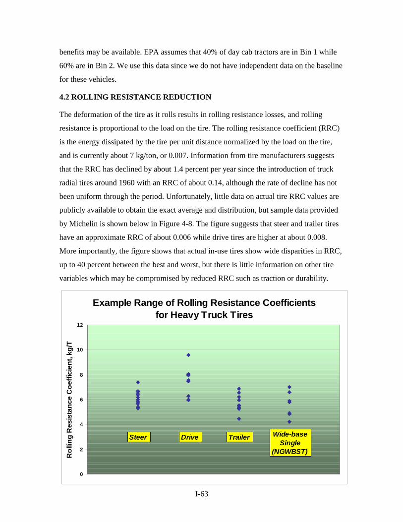
I-63

benefits may be available. EPA assumes that 40% of day cab tractors are in Bin 1 while

60% are in Bin 2. We use this data since we do not have independent data on the baseline

for these vehicles.

4.2 ROLLING RESISTANCE REDUCTION

The deformation of the tire as it rolls results in rolling resistance losses, and rolling

resistance is proportional to the load on the tire. The rolling resistance coefficient (RRC)

is the energy dissipated by the tire per unit distance normalized by the load on the tire,

and is currently about 7 kg/ton, or 0.007. Information from tire manufacturers suggests

that the RRC has declined by about 1.4 percent per year since the introduction of truck

radial tires around 1960 with an RRC of about 0.14, although the rate of decline has not

been uniform through the period. Unfortunately, little data on actual tire RRC values are

publicly available to obtain the exact average and distribution, but sample data provided

by Michelin is shown below in Figure 4-8. The figure suggests that steer and trailer tires

have an approximate RRC of about 0.006 while drive tires are higher at about 0.008.

More importantly, the figure shows that actual in-use tires show wide disparities in RRC,

up to 40 percent between the best and worst, but there is little information on other tire

variables which may be compromised by reduced RRC such as traction or durability.

Example Range of Rolling Resistance Coefficients for Heavy Truck Tires

0

2

4

6

8

10

12

Rol

ling

Res

ista

nce

Coe

ffici

ent,

kg/T

Steer Drive Trailer Wide-baseSingle

(NGWBST)

I-64

The use of higher RRC tires on the drive axle does suggest that some compromise

between traction and RRC is possible for a given level of technology. For example “rib”

tires with straight tread grooves have lower RRC than “block” or “lug” tread designs but

also have lower traction and are typically used on trailer axles. However, there is

significant variation in RRC even within specific axle groups and tire tread designs; for

example, some newer drive tires with continuous shoulder ribs can have lower RRC than

trailer tires. In addition, the weight loads on the axle groups are different, and this leads

to different sensitivity to RRC reduction. For example a properly loaded 5-axle tractor

trailer will have 42 + 2% of the load on each dual axle group and 16 + 1 % on the front

axle, but because of the higher RRC tires used on drive axles, they can account for about

50% of tire energy loss with the trailer axles accounting for 35% and the front axle

accounting for 15%.

The EPA SmartWay program certifies tires that meet a maximum RRC level, which are

currently specified as 5.8, 7.3 and 5.2 kg/ton for the steer, drive and trailer axles,

respectively. Anecdotal information from truck manufacturers suggests that about half of

all trucks are using tires that meet or exceed these specifications as of 2009, but the

picture on trailer tires is less clear. These values may be close to the averages for Class

8B vehicles (tractors). If the averages decline at the historic rate of 1.4% per year, then

the 2020 values will be 5 and 6.25 kg/ton respectively, which are equal to the lowest

values shown in Figure 4-8. There appears to be no specific lower limit for 2025

proposed by tire manufacturers by axle type but the historical rate suggests a reduction of

20% to 4.64 and 5.84 kg/ton, though some studies such as those by NESSCAF and TIAX

have asserted a lower value of 4 to 4.5 as feasible before 2020 for all axles.

The “Wide Base Single” tire has been offered by Michelin since the 1980s, and a New

Generation version has been offered since 2000. Michelin has claimed that this tire can

replace the dual tires employed on drive and trailer axles and their Single tire has 20

percent lower RRC than the best dual tire option. Current data shows some super single

tires near the 4.0 kg/ton value, but it is not completely clear if the test methods to

determine rolling resistance are identical across manufacturers. In addition, the lower tire

I-65

and rim weight can save 700 pounds with Aluminum rims, and possibly more with steel

rims, and net cost on a new truck is lower due to the savings on the rims. In spite of these

claimed advantages, the wide base single tire technology has achieved a market

penetration of under 10% in 2009 according to truck manufacturers. One reason is that

these tires do not offer “limp home” capability in the event of a tire failure while dual tire

system could provide such capability in emergencies. Specific truck manufacturers also

stated that some fleet owners experienced very little fuel savings when switching from

low rolling resistance dual tries to wide base single tires. Finally, some states do not

allow such tires on oversize/ overweight loads, so truck owners are cautious about using

these tires. However, the wide base singles appear to reduce RRC by an additional 20

percent over a similar technology regular tire.

The effect of a 10 percent RRC reduction is readily derived from the sensitivity

coefficients shown in Table 2-1. For a long haul truck, a 10 percent RRC reduction

results in 3.5% reduction in fuel consumption at constant engine efficiency, but engine

efficiency decreases slightly due to the lower average load so that a slightly lower

number is expected. On a regional route, the same 10 percent RRC reduction results in a

2.15 percent fuel consumption decrease at constant engine efficiency. Michelin also

provided data on the measured values from reducing RRC by 20 percent as shown here:

The regional cycle full loaded data shows a 3.7% decrease as opposed to the expected

4.3% and the long haul cycle shows a 6 percent decrease in fuel consumption as opposed

to the 7% predicted, indicating that efficiency losses in the engine reduce the expected

value by 15% in both cases (from 7 to 6 and 4.3 to 3.7). Hence, the anticipated 20%

reduction in RRC between 2009 and 2025 should result in a 6% decrease in fuel

consumption on the long haul cycle and a 3.7% decrease on the regional cycle. The

CRR=5.5kg/t CRR=4.5kg/tSub Urban Use – half loaded 16.53 gal/100mi 15.98 gal/100mi 0.55 gal/100mi 3.3%Regional Use – half loaded 15.13 gal/100mi 14.53 gal/100mi 0.59 gal/100mi 3.9%Long Haul Use – half loaded 12.62 gal/100mi 11.94 gal/100mi 0.68 gal/100mi 5.4%Sub Urban Use – full loaded 21.29 gal/100mi 20.57 gal/100mi 0.72 gal/100mi 3.4%Regional Use – full loaded 19.76 gal/100mi 19.04 gal/100mi 0.72 gal/100mi 3.7%Long Haul Use – full loaded 14.92 gal/100mi 14.02 gal/100mi 0.89 gal/100mi 6.0%

Heavy Truck (40t) 12.0l Diesel engine

Fuel Consumption Fuel Savings Percent

I-66

Michelin data also shows the reduced effect of RRC when the truck is not fully loaded,

and the benefit of RRC reduction is reduced by 10 to 15 percent when moving from full

load to half load. On the vocational truck cycle, the benefits of RRC reduction are quite

small, with a 10 percent reduction yielding a maximum 0.8% fuel consumption benefit

and an expected 0.68% benefit.

Costs of reduced rolling resistance are difficult to estimate since many tire attributes vary

simultaneously. Cost increments estimated by TIAX are based on super single tires but

appear to include the cost of aluminum rims (which reduce weight but not rolling

resistance). According to manufacturers, the tires with Smart-Way specification typically

cost $50 to 100 more per tire on average than uncertified tires and we have utilized this

number ($75 + 25) for a 10% RRC reduction, and $150 for a 20% RRC reduction per

tire. Costs of the Single Wide Base Tire are small to negative if the cost of the rims are

included and hence all of the cost is associated with the hedonic cost of uncertainty about

limp home potential and resale value.

4.3 WEIGHT REDUCTION

The reduction in truck empty weight can have a beneficial effect on fuel economy or on

the payload specific economy (payload ton miles per gallon) if the weight reduction is

offset by increased payload. However, only a small fraction of trucks operate at the GVW

limit at any given time and it appears likely that about 90 percent of trucks will have a

fuel economy benefit from weight reduction. Weight affects both the inertial energy lost

to the brakes and tire rolling resistance. With increasing speeds, the inertial loss

component goes down as the tire component increases so that the sum of the two is near

constant between 20 and 50 mph at 45 to 48%. At very low speeds (~5mph) the inertial

component is dominant, but at speeds higher than 50 mph, the aerodynamic component

becomes the largest single source of energy loss.

For a typical tractor trailer unit, the tractor (day cab) weighs about 14,000 pounds and the

53 foot steel trailer weighs about 13,000 pounds. Sleeper cab units are about 3000 to

4000 pounds heavier, so that the tractor-trailer combination weighs 27,000 to 31,000

pounds. Typical operating weight is about 75,000 pounds, so that a 1000 pound weight

reduction is a 1.33% decrease of total weight but a 3.4% decrease of empty weight. As

I-67

noted, weight accounts for 47.5% of energy use on the long haul cycle and on the

regional cycle, so that a 1000 pound weight reduction corresponds to a 0.64% fuel

economy increase at constant engine efficiency or a 0.54% increase with a 15%

efficiency loss factor as for tires. This number corresponds well with data reported from

SmartWay (which reports impacts from 0.4 to1.0 percent) and the NESCCAF simulation

study which reports 0.5%. The Aluminum Association also reported that a 10 percent

empty weight reduction corresponds to a 1.6% fuel economy benefit which is

proportional to the benefits we derived for the 3.5% reduction.

Medium-duty trucks in Class 6 and 7 weigh about 14,000 + 1000 pounds for a van body

unit and operate at 24,000 pounds (class 6) to 30,000 pounds (class 7) loaded weight.

Hence, a 500 pounds. weight reduction corresponds to a 2.1% weight decrease for a Class

6 truck to a 1.7% reduction for a class 7 truck, with fuel economy impact of about 1%

and 0.8% respectively. Data from manufacturers suggest that the 0.8 to 1 percent range is

appropriate for this level of weight reduction.

Weight Reduction Through Material Substitution

Weight reduction is possible both through improved design and through the use of

alternative materials, notably composites and/or aluminum. It is now common for cabs to

have composite fenders, hood and aerodynamic aids such as the roof deflector and side

flares. (Of course, the aerodynamic add-on devices add weight). However, most

structural parts are still made of steel. Widespread use of high strength steel and weight

efficient design can reduce weight; for example, MAN has introduced the new TGX

series that saves 200 to 270 pounds relative to the older TGA series through improved

design and use of high strength steel. The replacement of the twin leaf springs for the

front axle with a single parabolic leaf alone resulted in a 100 to 120 pounds. weight

saving. The use of HSLA in suspension components in the rear axle saves about 50 to 60

pounds

In addition, the 12L engines now common in most long haul trucks save about 300 to 400

pounds relative to the older 15L engines. The newest generation of trailers uses

composites and high strength low alloy (HSLA) steel and are 1000 to 1500 pounds lighter

I-68

than older all steel trailers. At the same time, we note that many of these improvements

are now incorporated into the majority of new trucks and are hence in the baseline.

For analysis purposes, we have separated truck empty weight reduction into four steps:

- A 5% weight reduction from weight efficient design and extensive use of

HSLA steels as well as a smaller displacement engine. Most trucks introduced

in the 2007+ time frame already incorporate these improvements although the

state of the trailer market is less well understood.

- A 10% weight reduction from the use of composites for body closures, floor

panels and exterior panels, as well as aluminum in some castings and forgings.

Some Class 8B trucks that emphasize weight reduction already offer these

improvements in new models

- A 15% weight reduction from aluminum or composite use in structural

members such as the frame rails. Aluminum frame rails can save 900 to 1000

pounds if used on both tractor and trailer in a Class 8B truck, for example, and

are offered in specific applications like a fuel tanker which operates at

maximum allowable GVW.

- A maximum 20% weight reduction with a highly intensive weight reduction

design employing both aluminum and composites. This is based on inputs

from manufacturers, who see this level as technically achievable but not cost-

effective now.

Each step in the weight reduction ladder corresponds to 600 to 700 pounds weight

reduction for a Class 6/7 van body truck and a similar level of weight reduction for the

tractor and trailer (each). In a recent analysis of light duty vehicle weight reduction, we

have estimated the cost of material substitution per pound saved as $0.75. $1.50, $2.50

and $4 per incremental pound saved in each step. For a class 8 tractor, this would amount

to $490, $1470, $3100 and $5700 respectively with similar amounts for the trailer.

I-69

I-70

5 FUEL SAVINGS FROM OPERATIONAL IMPROVEMENTS

5.1 OVERVIEW Unlike light-duty vehicles, there is significant potential to reduce fuel consumption by

increasing the operational efficiency of moving goods. These improvements can be

summarized as follows

- reducing empty backhaul

- preventing over-speeding on the highway

- use of adaptive and predictive control

- improved driver training to drive in a fuel efficient manner

- maintaining proper tire pressure

- using double trailer combinations or longer trailers

- mode shifting from road to rail (inter-modal transport)

- Idle reduction

These operational items and their potential benefits are not the focus of this report but are

mentioned here, as many analyses of fuel savings from heavy-duty trucks have combined

operational savings with technology based savings. Only idle reduction can be facilitated

with technology and considered in more detail in Section 5.3, but all other issues are

summarized below.

5.2 SUMMARY OF POTENTIAL SAVINGS FROM OPERATIONAL

IMPROVEMENTS

Reducing empty backhaul for heavy-heavy duty trucks can be achieved by better load

and route matching but there is obviously an irreducible minimum since some amount of

empty mileage is necessary as the delivery point and pickup of new loads will never

occur at the same location. The 2002 VIUS data shows that empty backhaul accounts for

I-71

33 percent of VMT and about half that percentage of fuel consumption since trucks are

substantially more fuel efficient when empty. Since 2002, there has been a proliferation

of private load matching services and route optimization services based on the internet

and on GPS based truck position sensing. Anecdotal evidence suggests that empty

backhaul has declined since 2002 to less than 25%, and that load clearing market is

already quite efficient. Hence, further fuel savings from reducing empty backhaul may be

quite small and probably account for less than 5 percent fuel saving potential.

Preventing over-speeding on the highway has been shown to provide significant fuel

savings. Reducing the speed from 70 mph to 65 mph (or 7.1%) results in a 6 percent fuel

economy improvement. For a vehicle operating 100,000 miles per year at a base fuel

economy of 6 mpg, fuel cost with diesel at $3 per gallon is $50,000 annually. Hence, a

six percent fuel economy improvement saves about $2830 annually. Unfortunately truck

productivity is also reduced since the distance traveled per day is reduced. Trucks do not

operate at 70 mph all the time and assuming a peak to average speed ratio of 1.75, the

reduction of peak speed by 7.1% will reduce truck productivity by 4.1%. A HHDT

typically produces revenues of $180,000 to $250,000 per year implying a productivity

loss of $7350 to $10,200, substantially higher than the fuel savings. This is the major

reason why truckers speed; the economic incentives are too strong even at higher fuel

prices. We do not anticipate any fuel savings from voluntary speed reductions. However,

the EPA has proposed providing credits for hardwired speed limiters set at 63 mph or 60

mph. The credit provided for sleeper cab equipped trucks is quite large due to the EPA

assumption that 85% of their VMT, these trucks operate at 65mph constant speed.

Driver training can have a significant impact on fuel economy on-road. The American

Trucking Association (ATA) Maintenance Council estimates that the best drivers

compared to the worst drivers can improve fuel economy by up to 35% but this is an

extreme comparison; other studies have estimated impacts in the 5% to 15% range. In

addition to limiting speed and idling time, drivers can improve fuel economy by

improved gear shifting, acceleration practices, route choice and use of accessories. Due to

the overlap with speed and idling issues considered separately (which accounts for much

of the fuel economy benefit), we selected 4% as a possible maximum benefit from driver

training, and have assumed that about 50% of drivers (mostly employed by large fleets)

I-72

have already had the training. Costs of driver training programs are estimated at $1400

based on data from ATA.

Maintaining proper tire pressure improves fuel economy since under-inflation by

10psi increases rolling resistance by 7% which reduces fuel economy by about 1.5 to 2%

if all tires are under-inflated by this amount. Of course, under-inflation may vary across

tires on a given truck, and EPA has estimated from limited survey data that the net

average of proper inflation is to increase fuel economy by 0.6% for the fleet as a whole.

New tire pressure monitoring systems are available for the approximate cost of $40 per

tire + $100 for the monitoring system.

Shifting to larger trailers or using combinations of trailers called long combination

vehicles (LCV) is always more efficient in terms of fuel use per ton-mile of payload

transported. While this is widely recognized, many states and local areas restrict the use

of multiple trailers that involve the use of two or three trailers of differing lengths

(depending on state) that are currently used in some states. Indeed, the trucking

community refers to these as “Turnpike doubles” or “Rocky Mountain doubles” and

“triples”. LCV use is governed by federal law. Prior to 1991, states could set their own

laws with regard to trailer length maximums and combination maximums. After a

handful of (western) states starting increasing the maximum trailer limits the federal

government stepped in and has governed the maximums for the interstate highway

system, effectively governing all use. However states that had already increased their

maximums were grandfathered into the new system and the old maximums are still

allowed in those states. An allowed double is a combination of two 28-foot trailers, but

this has limited application since it isn’t much bigger than a single 53-foot trailer that is

standard. It is used for specific operational requirements where an operator will need to

drop one trailer and carry the next to another destination (for example, Fed-Ex or UPS).

The use of many double combinations increases payload based efficiency by 12 to 25%

based on measured values, but are often opposed based on safety grounds as it makes

passing on narrow roads much more hazardous, and on access due to maneuverability

issues. However, a change in federal law can widen usage to major routes, and assuming

that the shortest double trailer combination (the Rocky Mountain double) is allowed, fuel

I-73

usage can be cut by 15% on approximately 60% of HHDT. This is a “zero cost” option if

social and safety issues are not considered

Inter-modal freight has received wide attention in recent times. It is widely known that

goods movement by rail or barge is much more energy efficient and rail can use one-

tenth of the energy of trucks if the routes are identical and delivery is not time

constrained. It is very difficult to generalize this to any specific load and route, since the

route circuity on rail and the distance of the rail head from the pick up and delivery points

strongly affect these comparisons of energy use. Increased use of barges is, of course,

limited by available waterways. Road-to-rail has been increasing significantly for goods

(typically commodities such as grain, ores, fertilizer, cement, etc.) where the market

forces do not place a premium on time sensitivity, and the 2002 VIUS shows that bulk

goods and commodities account for only 4% of trucking payloads. Hence, it appears that

the market for road-to-rail is quite efficient and further significant movement in this

direction may not result in large fuel savings.

5.3 IDLE REDUCTION

Idle reduction has received considerable attention form EPA and CARB with reference to

criteria pollutants, but is also an energy issue. Surprisingly little data exists on the actual

extent of long idles in practice; the EPA estimate of 8 hours a day for 300 days a year for

all HHDT appears to be very much higher than any trucking industry estimate. Many

long distance trucks do keep their engines on at night when the trucks feature a sleeper

cab to provide space conditioning, but some trucks are kept running under very cold

winter conditions because of problems starting a large diesel engine in very cold weather

(typically below -10 C).

There are several technology options to reduce fuel use during idling including

• Direct-Fire Heaters, which heat the cab and engine using a small flame and a heat

exchanger. This technology has only around 5% market penetration in US vs.

55% in Europe.

• Auxiliary Power Units (APU), which are a secondary combustion engine

connected to a generator to power electrical systems and provide heat. They have

I-74

near zero market penetration due to concern about overloading existing wiring

systems and retrofits rendering void the truck’s warranty.

• Automatic Engine Idle Systems, which run the engine only to maintain set cabin

temperature and battery voltage, and can automatically shut off and restart the

engine to minimize fuel use. They are offered as an option of new truck purchases

from some manufacturers but some drivers can find engine restarts disruptive

while sleeping. They are currently installed in trucks that account for 7-8% of

VMT.

• Truck Stop Electrification, which taps the electrical power grid to power the

truck’s auxiliary units while at overnight stops. This technology requires a

properly equipped station with a “shore power” port as well as additional wiring

and equipment on the truck. Stations are rare with implementation suffering from

a ‘chicken or the egg’ problem as stations don’t see a market until enough trucks

are equipped, while the added cost of the equipment for trucks does not pay back

without a sufficient station network.

• Advanced Truck Stop Electrification which provides cabin heating and cooling

from an external source via air supply and return pipes as well as power outlets

for driver accessories. A pilot project (IdleAire Technologies) charges $1.20 per

hour to truckers and installs at stations at no fee to the station operators.

Based on the cost-benefit analysis shown below in Table 3-1, we have considered engine

idle systems, direct fire heaters and APU power as possibilities for fuel conservation.

Truck Stop Electrification is very cost effective but could require significant market

intervention to make it widely available.

I-75

Table 3-1: Costs and Benefits of Idle Reduction Strategies

Fuel Reduction Emission Reduction (kg) Maint. Operating Payback

Period Technology Initial Cost Gallons percent CO2 Nox PM-10 Savings Charge (months)

Direct-Fire Heater -$2,000 690 4.3% 7,000 121 N/A $210 $0 19

Auxiliary Power Unit -$7,000 1,320 8.1% 13,392 166 2.5 $336 $0 36

Automatic Engine Idle -$1,250 900 5.6% 9,131 97 2.1 $168 $0 10

Plug-in TSE -$2,800 1,800 11.1% 11,613 179 4.1 $336 -$745 15

Advanced TSE -$25 1,800 11.1% 11,613 179 4.1 $336 -$2,880 2

Note: All costs reflect the perspective of the truck owner. Advanced TSE can provide services that may have to be paid for separately, such as Internet access. The value/savings of such non-fuel related services is not reflected here.

From ICF draft report – January 2002

Most of the operational improvements are also not relevant for these classes of trucks

except for the automatic engine idle and driver training related benefits. Of course, cost

effectiveness for all technologies are quite different due to the different annual miles of

travel and different use patterns but these are accounted for in the calculations shown in

Section 6.

I-76

6 FUEL ECONOMY POTENTIAL AND COST EFFECTIVENESS ANALYSIS

6.1 OVERVIEW

This Section provides an integrated view of the fuel savings and costs possible from an

analysis of scenarios of all truck technologies operating together on various truck weight

classes, and different duty cycles. However, our detailed discussion of truck operating

characteristics and technologies in the previous sections show that

- every weight class of trucks has a range of different truck types operating

different duty cycles

- the current technology and fuel economy baseline for 2008/9 is not well

understood

- costs of truck technology vary over broad ranges and by vehicle type.

Hence, the analysis presented in this section targets some specific functional areas where

there are significant truck populations based on the VIUS survey data and allocates them

to one of three duty cycles that are based largely on manufacturer inputs. In addition,

baseline technology levels are based on manufacturer comments on sales in 2008/9. The

cost issue was tackled by allocating technologies into broad payback categories that were

more easy to determine than specific costs. The data and methodology employed to make

these distinctions are described below.

6.2 NEW TRUCK SALES ALLOCATIONS BY CLASS AND APPLICATION

New heavy-duty truck sales have varied significantly over the last 5 years with the

medium trucks in classes 5 through 7 varying form as much as 180,000 units to as low as

100,000 units. class 8 trucks sales have also varied form a high of 275 thousand units to a

low of 128 thousand units during the period. These large variations were in part due to a

“pre-buying” rush to beat the emission requirements for 2007 and exacerbated by the

I-77

recession in 2008. We anticipate future sales of about 140,000 units in the 2012 to 2015

period for medium duty trucks and sales of 225,000 Class 8 trucks. About 30% of Class 8

units are straight trucks (class 8A) in the 40,000 to 60,000 pound GVW category

primarily used in rough-duty applications like refuse haulers, agricultural goods carrier

and construction support (all 3 axle trucks are over 33,000 pounds GVW). The remaining

70 percent of class 8 vehicles are tractor-trailer units with GVW over 60,000 pounds or

class 8B, and these are typically the focus of most analyses due to their high annual VMT

Such trucks are used in long haul and regional haul applications, with a relatively small

percentage in rough duty and short haul applications. About 60% of these feature sleeper

cabs and 70% have enclosed van bodies. The splits between cab type and body type for

new trucks, based on industry information, is as follows as a percent of entire Class 8B

fleet:

Cab Type Sleeper Day cab

Van body 50% 20%

Tanker 2% 4%

Flatbed/Dump 8% 16%

The VIUS survey data lists the typical radius of operation in steps of 0 to 50 miles, 50 to

200 miles and over 200 miles, and the percentage of Class 8B trucks in the longest radius

of operation is only 17.1% but the 50 to 200 miles segment is at 34.1%, and the average

annual VMT for the van body tractor trailer is 112,500 miles and 82,000 miles for each

segment suggesting that the mid-range operations also may entail some sleeper cab use.

Moreover, the percentages of the fleet are different from the percentages of new trucks in

this class since trucks are used intensively in the first 4 to 6 years and then sold to second

owners who use the more in regional and short haul applications. According to industry

sources, the average VMT of sleeper cab equipped trucks is in the 95,000 + 10,000 miles

per year range while the annual VMT for day cab trucks is about 50,000 + 10,000 miles

across different body types. However, new vehicles less than 5 years old average 120,000

miles a year for the van body tractor trailer according to Vehicle Inventory and Use

I-78

Survey (VIUS) data, and this is relevant for many of the calculations of cost

effectiveness.

Medium duty trucks (classes 6, 7 and 8A) have much lower annual VMT and van body

trucks account for about 30 percent of all trucks according to both manufacturers and the

VIUS data. About 70 percent of all trucks are used short haul applications while about

20 percent are used in regional haul, with the remainder in rough duty or vocational

applications. In general the trucks used in regional applications average 20,000 miles a

year while the trucks in short haul applications average only 12,000 miles per year.

Vocational trucks average even lower annual VMT between 5000 and 10,000 miles per

year. Trucks under 5 years old have somewhat higher average VMT at 28,000 miles per

year for regional applications and 18.000 miles per year for short haul. These values are

used to compute cost effectiveness to the buyer.

6.3 EVALUATIONS OF COST EFFECTIVENESS

The technology discussion in sections 3 and 4 pointed to the fact that technology costs

were not well defined except in isolated instances, and also varied considerably in many

cases by truck size and application. Hence, the development of a traditional supply curve

of technology improvement to fuel economy versus cost is difficult to establish in a

manner similar to that for cars. However, it is widely recognized that most long haul

truck buyers demand a that costs of technology be paid back from fuel savings in 3 years

or less so that full cost recovery is guaranteed within the period of first ownership which

is usually 4 to 5 years before resale. It is not clear if the same payback requirement exists

for medium duty trucks but manufacturers believed that this would be a useful

approximation of market demand to examine payback periods of five years as being more

representative. In addition, manufacturers were more willing to provide inputs on

payback period in a general sense than to discuss specific cost data and industry

discounting practices. Hence, we classified technologies by “payback period” where the

payback was determined by the undiscounted value of fuel saved (at $3/ gallon) relative

to the incremental price of technology into three categories:

- a period of 3 years or less implying that normal market forces would be

sufficient for technology introduction

I-79

- a period of 4 to 6 years, implying marginal cost-effectiveness at current

conditions, but some of these technologies could be adopted by the market if

fuel prices increase or standards would require such technology

- a period greater than or equal to 7 years, implying technologies unlikely to be

adopted by the consumer absent subsidies or severe market forcing conditions.

These payback periods correspond to the following approximate price limits per percent

fuel savings for the three categories in different applications, and should be treated as

indicators rather than as exact numbers:

Value of 1% Fuel

Consumption reduction

Total VMT

3/6 years

3 year

payback

6 year

payback

Long haul tractor trailer 360K/600K $1800 $3000

Regional Haul tractor

trailer

180K/300K $900 $1500

Regional haul medium

duty

84K/125K $280 $420

Short haul medium duty 60K/100K $225 $375

Vocational trucks 30K/48K $120 $190

As can be seen, there is almost a 15 to 1 range in allowable price increase per percent fuel

savings depending on application, illustrating the difficulty of commenting on cost and

feasibility without specific reference to a baseline and usage type. In addition, the same

technology can be classified at very different levels of cost-effectiveness depending on

application. These issues are addressed for the heavy –heavy and medium heavy

segments separately in the following sections.

6.4 CLASS 8B HEAVY-HEAVY DUTY POTENTIAL

As noted in Section 6.2, the long-haul and regional haul segments of the Class 8B fleet

account for most of the population and over 95% of fuel use in this segment.

I-80

Technologies have been organized into four categories: those necessary for emission

control, those likely to be adopted by the free market ( 3 years or less payback),

marginally cost effective technologies ( 4 to 6 year payback) and cost-ineffective

technologies. Drive train and body technologies are shown in the two tables below.

Table 6-1 shows the drive train technology improvements over the 2008 – 2017 and 2008

– 2025 time frames. The 2010 introduction of urea/SCR has a very significant effect in

the short term with emission control related technology providing a 5.4% reduction in

consumption by 2017 and a 9.2% related reduction by 2025 assuming constant emission

standards. The non urea emission control system is expected to result in a fuel efficiency

loss of about 2.5 to 3 percent relative to the urea/SCR system and the route also precludes

mechanical turbo-compounding due to the sequential turbo requirement, although organic

Rankine cycle based heat recovery will be possible Urea consumption is at about 2 to 2.5

percent the diesel consumption rate. Hence, our analysis shows that the non-urea route

could be competitive in regional haul category where mechanical turbo-compounding

produces very small benefits, as long as urea prices are higher than diesel fuel prices

(they were almost $6 per gallon recently). However, it is less competitive in the long haul

category, at least for the short term when mechanical turbo-compounding is widely

introduced, but may be competitive if the Rankine bottoming cycle is introduced. It is

also notable that the free market forces will likely bring about half to two thirds of the

total drive train improvements possible.

The benefits of reducing truck tractive energy requirements from drag, weight and rolling

resistance reduction are more complex in terms of cost effectiveness. Classification of

many improvements into payback categories is very problematic due to three issues.

First, there are many more trailers than tractors, and the registered population ratio is

about 2.8, but this masks a lot of variability around the average for individual fleets. In

addition, there are reportedly a large number of lightly used old trailers, so that newer

trailers may have a much larger fraction of miles traveled. We have assumed an “active

trailer” to tractor ratio of 2 to estimate costs and effectiveness of technology applicable to

trailers. Second, many devices have operational issues and concerns that has prevented

significant market penetration, and we can associate this with a hedonic cost that must be

added to the real cost. Third, the effectiveness of some aerodynamic aids on trucks with

I-81

Table 6-1: Potential Class 8B Fuel Consumption Reduction (%) from Drive Train

Technology

2017 2025

Long haul Regional Long haul Regional

2500/3000 bar FI 0 0 1.0 1.0

Seq. Turbo +downsize 0 0 0.5 1.0

Urea/SCR 3.0 2.0 5.0 4.0

Cooled EGR 1.0 1.0 1.5 1.5

Closed Loop FI 1.5 1.0 3.0 2.0

Emission Control Total

with/ without urea 5.4/ 2.5 4.0/ 2.0 9.2 / 5.9 7.3/ 5.4

Variable valve actuation - - 1.0 1.0

Mech. Turbo-compound 2.5 - 3.0 -

Engine Friction 1.0 1.5 1.5 2.2

12-speed + Direct drive 1.5 1.0 1.5 1.0

Engine+ axle lubricants 0.7 1.0 1.0 1.5

Improved Accessories 0.5 0.8 0.7 1.0

3 year payback tech. 6.05/ 3.65 4.25 8.4/ 5.6 6.55

Mech. Turbo-compound - 1.3 - 1.5

Electric Acc. Drive 1.5 2.2 1.3 2.0

Automated Manual Tran. 3.0 5.0 3.0 5.0

Electric Turbo-compound

or Organic Rankine 2.5 - 3.5 or 6.5

w/o urea 3.3 w/o urea

4 – 6 year payback tech, 6.85/4.45 8.3 7.6 / 10.5 8.2 /11.05

Electric Turbo-compound - 1.2 - 1.8 w/ urea

Hybrid 50kW drive 3.5 7.0 4.5 9.0

>6 year payback tech 3.5 8.1 4.5 10.65/ 9.0

Total Potential With/ without urea

20 / 13.3 22.5 / 18.9 26.6 / 24.1 29.0 / 28.45

I-82

non-van body trailers is not well understood and we have the used same benefits or

aerodynamic cabs and trailer skirts for both body types as a first approximation. The

estimation of hedonic cost is simply based on the classification by payback and current

market share. For example, the use of trailer skirts at a cost of $1500 to 2000 to produce a

3 percent fuel consumption reduction is cost effective in a 3 year time frame for long haul

trucks (after accounting for 2 trailers per tractor) but actual market penetration is low at

around 5%. This would correspond to a 5+ year payback so that the hedonic cost is

approximately equal to the actual cost and total cost is double actual cost. The available

technologies and payback classifications are shown in Table 6-2.

There are several major findings related to the data shown in Table 6-2. Unlike the fact

that drivetrain technology benefits are comparable for the long haul and regional cycles,

the benefits of body technologies are significantly higher for the long haul case than the

regional haul case, and in the van body case relative to the non van body case. This is due

to the fact that aerodynamic aids and reduced tire rolling resistance have a much larger

effect at highway speeds than at city/suburban speeds, and many aerodynamic aids like

the gap treatment and boat tail are applicable only to van body trailers. Second, the

negative hedonic aspects of some technologies distort the standard computations of cost-

effectiveness and many technologies that are relatively inexpensive have market

penetrations that suggest high hedonic cost. Determining market resistance to these

technologies in the future is still a challenge. Third, only about 40 to 45 percent of the

total available benefit is in the 3 year payback category, suggesting that a majority of the

benefits available will not be used in a free market scenario.

Idle reduction benefits outside of short term idle reduction from hybridization are not

directly considered in the tables, since it applies only to the subset of long haul Class 8B

vehicles with sleeper cabs where the HVAC is provided by engine power. As noted,

anecdotal information has been used to estimate that idle fuel consumption for these

vehicles can account for 8 to 10 percent of total fuel use, and the use of auxiliary power

units or externally supplied air can reduce the fuel use by 50 to 100 percent. This finding

is independent of engine energy used to overcome tractive force during driving and can

be accounted for separately.

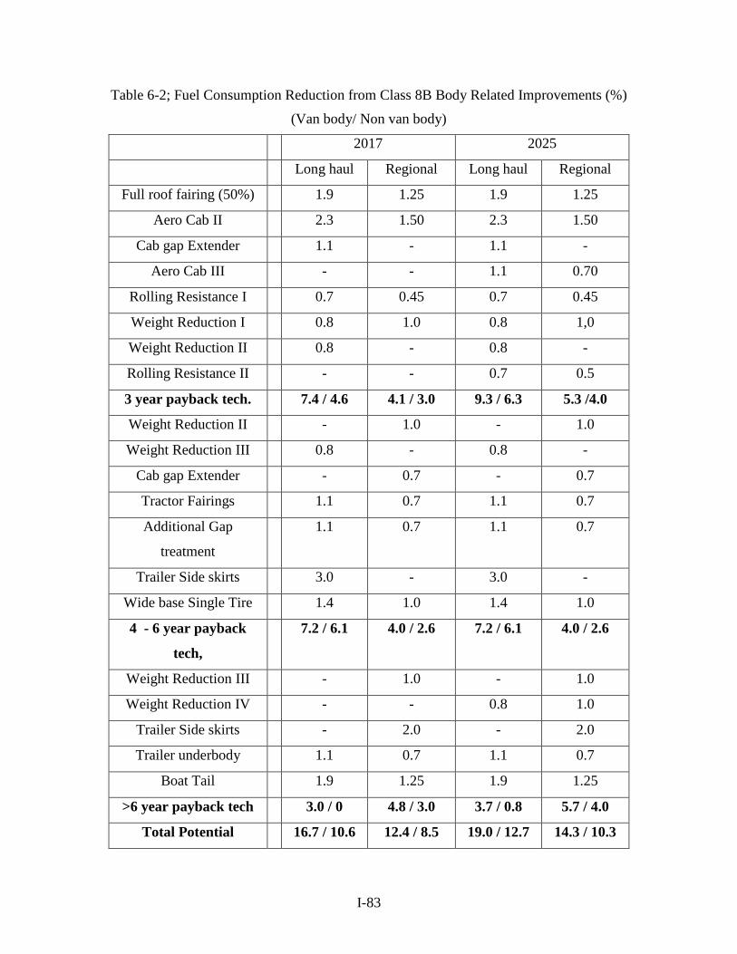
I-83

Table 6-2; Fuel Consumption Reduction from Class 8B Body Related Improvements (%)

(Van body/ Non van body)

2017 2025

Long haul Regional Long haul Regional

Full roof fairing (50%) 1.9 1.25 1.9 1.25

Aero Cab II 2.3 1.50 2.3 1.50

Cab gap Extender 1.1 - 1.1 -

Aero Cab III - - 1.1 0.70

Rolling Resistance I 0.7 0.45 0.7 0.45

Weight Reduction I 0.8 1.0 0.8 1,0

Weight Reduction II 0.8 - 0.8 -

Rolling Resistance II - - 0.7 0.5

3 year payback tech. 7.4 / 4.6 4.1 / 3.0 9.3 / 6.3 5.3 /4.0

Weight Reduction II - 1.0 - 1.0

Weight Reduction III 0.8 - 0.8 -

Cab gap Extender - 0.7 - 0.7

Tractor Fairings 1.1 0.7 1.1 0.7

Additional Gap

treatment

1.1 0.7 1.1 0.7

Trailer Side skirts 3.0 - 3.0 -

Wide base Single Tire 1.4 1.0 1.4 1.0

4 - 6 year payback

tech,

7.2 / 6.1 4.0 / 2.6 7.2 / 6.1 4.0 / 2.6

Weight Reduction III - 1.0 - 1.0

Weight Reduction IV - - 0.8 1.0

Trailer Side skirts - 2.0 - 2.0

Trailer underbody 1.1 0.7 1.1 0.7

Boat Tail 1.9 1.25 1.9 1.25

>6 year payback tech 3.0 / 0 4.8 / 3.0 3.7 / 0.8 5.7 / 4.0

Total Potential 16.7 / 10.6 12.4 / 8.5 19.0 / 12.7 14.3 / 10.3

I-84

I-85

6.5 MEDIUM DUTY TRUCK TECHNOLOGY POTENTIAL

Almost all medium duty trucks in Classes 5 through 8A are straight trucks, with 2 axles

(classes 5, 6 and 7) or 3 axles (class 8A). As noted in section 2, very few are used in long

haul, and only a modest fraction, about 20 percent, are used in regional haul. The vast

majority are used in urban locations or as vocational trucks in utility and municipal fleets

or as buses. Due to the majority of such vehicles being used in low speed applications, it

is likely that technologies better suited for high speed full load situations such as turbo-

compounding or waste heat recovery may not be commercialized in the smaller

displacement engines ( 6 to 10 liters), although there may be some models offering an

optional turbo-compound versions.

Table 6-3 shows the benefits of drive-train technologies for vehicles operated on a

regional cycle or city/ vocational cycle. The engine technology benefits are assumed to be

similar for the city and vocational cycles as little data exists to accurately define the

differences in engine technology benefits over a 15 to 20 mph cycle versus a 5 to 10 mph

cycle with occasional high external power take off loads. However, the differences in

hybridization benefits between the two cycles are recognized in this analysis. Although

the benefits from engine technology alone are smaller for MDTs relative to the Class 8B

vehicles, the net benefits from all drive-train technologies are higher than for Class 8B

trucks due to the larger impacts of transmission and hybridization technology on the

lower speed cycles.

Table 6-4 shows the benefits of body technologies for MDTs and the benefits on the

regional cycle are comparable to those for Class 8B trucks, even though the aerodynamic

benefits are smaller. However, the impact of body technologies is very small for trucks

used in urban cycles or on vocational cycles since aerodynamics and rolling resistance

are smaller parts of overall fuel consumption. This also minimizes the issues related to

hedonic costs for trucks used in these applications.

I-86

Table 6-3: Potential MDT Fuel Consumption Reduction (%) from Drive Train

Technology

2017 2025

Regional City/Voc Regional City/Voc

Seq. Turbo +downsize 0 0 1.0 1.5

Urea/SCR 2.0 1.5 3.0 2.0

Cooled EGR 1.0 1.0 1.5 1.5

Closed Loop FI 1.0 1.0 2.0 2.0

Emission Control Total

with/ without urea

4.0/ 2.0 3.5/ 2.0 7.3/ 4.4 6.3/ 4.9

Variable valve actuation - - 1.0 1.0

Engine Friction 1.5 2.0 2.2 3.0

AMT (70% pen) 4.9 7.0 4.9 7.0

Engine+ axle lubricants 1.0 1.0 1.5 1.5

Improved Accessories 0.8 1.2 1.0 1.5

3 year payback tech. 8.0 10.8 10.2 13.35

Mech. Turbo-compound 1.3 0 1.5 0

Electric Acc. Drive 2.2 2.8 2.5 3.0

4 – 6 year payback tech, 3.5 2.8 3.9 3.0

Electric Turbo-compound 1.2 1.2 1.8 1.8

Hybrid 50kW drive* 12.0 20/30 15.0 24/35

>6 year payback tech 13.1 21 / 31 16.5 26.35 / 36.1

Total Potential

Hybrid without urea

25.2 32.9 / 40.3 29.5 41.1/ 48.9

*Additional work is required to better characterize hybrid benefits and duty

cycle dependence for trucks

I-87

Table 6-4: Fuel Consumption Reduction from Body Related Improvements (%) to Medium Duty Trucks

(Van body/ Non van body for Regional Trucks)

2017 2025

Regional City/Voc Regional City/Voc

Full roof fairing (50%) 1.25 - 1.25 -

Aero Cab II 1.5 0.4 1.5 0.4

Aero Cab III - - 0.7 0.2

Rolling Resistance I 0.45 0.15 0.45 0.15

Weight Reduction I 1.0 0.85 1.0 0.85

Weight Reduction II 1.0 1.0 -

Rolling Resistance II - - 0.45 0.15

3 year payback tech. 5.1 / 3.9 1.4 6.2 / 5.0 1.7

Weight Reduction II - 0.8 - 0.8

Weight Reduction III 1.0 - 0.8 -

Wide base Single Tire 0.9 - 1.4 -

6 year payback tech, 1.9 0.8 2.2 0.8

Weight Reduction III - 0.8 - 0.8

Weight Reduction IV - - 0.8 0.8

Side skirts 2.0 0.6 2.0 0.6

Boat Tail 1.25 - 1.25 -

>6 year payback tech 3.2 / 2.0 1.4 4.0 / 2.8 2.2

Total Potential 9.9 / 7.8 3.6 12.0 / 9.7 4.6

I-88

6.6 ABILITY TO MEET THE 2014/2017 STANDARDS

EPA has promulgated regulations for fuel economy and GHG emissions for heavy-duty

trucks, with a voluntary standard for 2014 and a requirement for 2017. The standards are

unusual in structure in that there is a separate standard for engines based on actual

measured BSFC on an engine dynamometer, and a vehicle standard that assumes a

“compliant” engine and models the effect of vehicle technologies using a simulation

model. The effect of transmissions cannot be accounted for in the current set-up and

hence EPA does not provide credits for transmission improvements. Vehicle technologies

are accounted for in a discrete manner in which specific improvement types are bundled

into “bins”. The test cycles over which fuel economy compliance is evaluated is

described in Section 2.5, and we noted the over-emphasis on the constant speed 55/65

mph modes for all trucks, and especially for sleeper cab equipped Class 8 trucks.

The engine standards are modeled in the regulatory analysis for the FTP and Steady State

(SET) modes, and the required improvement for heavy-heavy duty engines to 2017 is 5%

on the FTP cycle and 6.1% on the SET cycle, relative to 2010 baseline. In comparison,

this analysis in Table 6-1 shows that a 6.05% improvement is possible within a 3 year

payback(assuming that the 5% improvement related to urea/SCR implementation is

included in the 2010 baseline) but this includes some transmission benefits equal to 1.7%.

However, the benefits of turbo-compounding are much larger on the EPA cycle than our

2.5% estimate due to the high level of steady state operation, and we anticipate that

technologies with 3 year payback will be adequate or nearly adequate to meet the 2017

standard. For medium duty engines, the standard requires an 8.6% reduction relative to

2010. Table 6-3 shows that up to 10.8% is possible for city/ vocational cycles, with 3

year payback but 7% is transmission related so that only 3.8% is possible form engine

technology. In addition, we anticipate some improvements from emission control

technology and adoption of a downsized sequential turbo engine that was not in the 2010

baseline for some engines that could provide an additional 1to 1.5% benefit. The shortfall

would have to be made up with more expensive electric accessory drives, so that our

estimate of cost of compliance for the medium duty engines would be higher than EPA’s

estimate.

I-89

On the vehicle side, the medium duty vocational trucks are offered only one option for

improvement – tire rolling resistance reduction. The regulation allows credits for other

technologies such as hybrids, but requires the manufacturer to demonstrate the benefits

through actual testing. It is important to note that weight reduction and the use of the

AMT, which figure very prominently in Table 6-4 for improvements are not considered

in the EPA analysis.

In the case of long haul tractors, the regulations have several compliance options with

aerodynamic and tire improvements, idle limiters and speed control. The benefits for

these technologies are significantly higher than in our analysis due to the choice of the

long haul cycle at steady state. Figure 6-1 shows the different compliance options for the

long haul sleeper cab truck relative to the improvement required for 2017.

Figure 6-1: Technology Improvements for Class 8 Sleeper Cab Trucks for Compliance

The percentage reductions are very nearly similar to the CO2 g/ton-mile reduction

required since the baseline is 96 g/ ton-mile. The lowest drag aerodynamic tractor

available today coupled with the lowest rolling resistance tires is enough for compliance

but must be implemented across 100% of the fleet. Alternatives can include a 63 mph

I-90

speed limiter which provides a 3.2% benefit, or idle shutdown after 5 minutes which

provides a 5.2% benefit but these technologies carry substantial negative hedonic value

that is not considered by EPA. Using the more realistic cycles, obtaining the required

14.7% improvement would require use of all technologies with a payback of up to 6 years

from our calculations shown in Table 6-2. However, the overstatement of the benefit of

the technologies shown in Figure 6-1 is a major factor allowing compliance.

6.6 SUMMARY AND CONCLUSIONS

The information in Tables 6-1 to 6-4 has been aggregated to provide forecasts of fuel

consumption reduction by Class, Body Style and type of operation for the Class 8B

trucks and the Classes 5 to 8A trucks in tables 6-5 and 6-6 for 2017 and 2025,

respectively. The tables also show the cumulative technology benefit for fuel

consumption reduction as a function of the payback period, with the column labeled ECT

for emission control technology being independent of payback period as it is required by

regulation. One of the unexpected findings from the analysis is that the total available

benefit from technology is quite similar across all vehicle types (except vocational use

trucks) at 30 + 5 percent in 2017 and 39 + 5 percent in 2025. However, the distribution of

the benefits across payback period is quite different across the different combinations of

weight class, body style, and use type.

The relative importance of hybrid technology, which is quite expensive, is also

dramatically different, with hybrid technology accounting only for 11 percent of the total

available benefit (not 11% absolute) in the Class 8B Long-haul Van body Truck to almost

70 percent of the total available benefit in vocational use trucks. Hybrid technology or

trucks is still in its early development stages and refinement of this estimate is needed to

better estimate the future potential especially to the 2025 period. Note that these estimates

include the benefits of idle reduction in its definition of hybrid technology when the idle

is part of the drive cycle, but does not include benefits of idle reduction associated with

overnight use for sleeper cab trucks. The use of an auxiliary power supply unit or external

HVAC supply can reduce fuel consumption by another 4 to 6 percent based on anecdotal

estimates of annual use for overnight power.

I-91

The comparison of our results to those from the National Academy of Science’s recent

study of truck fuel economy is made difficult by the fact that the NAS study does not

provide an explicit baseline or drive cycle associated with its percent consumption

reduction estimates. In general, the NAS report includes the benefits of improved

operational strategies and idle reduction; when their estimates are adjusted for the two

effects, many of the numbers seem comparable. For example, the total benefit for tractor

trailers is listed as 51 percent reduction in consumption with 6 percent from operational

improvements another 4 to 6 percent from idle reduction (presumably overnight idle).

This suggests technology benefits of about 40 percent on a comparable basis, which is

very similar to our estimate. We are also less optimistic than the NAS on the pace of

technology introduction and believe that these reductions may be feasible in 2025 rather

than 2020, but even our estimate is an unprecedented rate of change for the truck

industry.

In terms of the newly promulgated standards, the study shows the following:

- The use of 65/ 55 mph steady state cycles without any gradient to quantify

fuel economy provides an incorrect picture of the real world benefits.

- The engine improvements required by EPA are those we consider likely to

happen under free market forces for the heavy-heavy segment, but are

aggressive for the medium duty segment

- Vehicle related improvements required for tractors in long haul operation

emphasize drag and rolling resistance reduction, as well as speed limiters but

their benefits are significantly overstated as a result of cycle choice.

- The benefits of weight reduction , transmission improvements and substitution

of the AMT for an automatic are largely ignored by the regulation but are very

relevant to the real world benefits, especially for medium-heavy trucks

I-92

APPENDIX A: DETAILED LISTING OF TECHNOLOGY IMPROVEMENT PROJECTIONS BY

PAYBACK PERIOD

I-93

Regional

Table 6-5 2017 Projections by Vehicle Class and Application

Hybrid Max.Wt. Class Operating Range Body Type 2008 MPG ECT Benefit % 3 yr, Payback 6 year payback Maximum Tech as % of max 2017 MPG

8B Long Haul Van (with urea) 6.00 5.40% 17.70% 28.86% 33.41% 10.48% 9.01

Van (w/o urea) 6.00 2.50% 15.18% 26.68% 31.37% 11.16% 8.74

8B Long Haul Non-Van (with urea) 5.72 5.40% 15.21% 25.84% 28.43% 12.31% 7.99

Non Van (w/o urea) 5.72 2.50% 12.61% 23.56% 26.24% 13.34% 7.75

8B Regional Van (with urea) 6.12 4.00% 11.85% 22.40% 32.11% 21.80% 9.01

Van (w/o urea) 6.12 2.00% 10.01% 20.78% 30.69% 22.81% 8.83

8B Regional Non-Van (with urea) 5.66 4.00% 10.84% 20.36% 29.01% 24.13% 7.97

Non Van (w/o urea) 5.66 2.00% 8.98% 18.70% 27.53% 25.43% 7.81

Medium Regional Van (with urea) 8.66 4.00% 16.18% 20.65% 33.26% 36.08% 12.97

Van (w/o urea) 8.66 2.00% 14.44% 19.00% 31.86% 37.66% 12.71

Non-Van (with urea) 8.82 4.00% 15.12% 19.65% 31.57% 38.01% 12.89

Non Van (w/o urea) 8.82 2.00% 13.36% 17.98% 30.15% 39.80% 12.63

Medium City All (w/o urea) 8.00 2.00% 13.81% 16.89% 35.26% 56.72% 12.36

Vocational All (w/o urea) 6.70 2.00% 13.81% 16.89% 43.46% 69.03% 11.85

I-94

Table 6-6 2025 Projections be Vehicle Class and Application

Hybrid Max.Wt. Class Operating RangBody Type 2008 MPG ECT Benefit % 3 yr, Payback 6 yr. payback Max. Tech % of max 2025 MPG

8B Long Haul Van (with urea) 6.00 9.20% 24.56% 35.31% 40.51% 11.11% 10.09

Van (w/o urea) 6.00 5.90% 19.43% 33.08% 38.46% 11.70% 9.75

8B Long Haul Non-Van (with urea) 5.72 9.20% 22.07% 32.38% 35.94% 12.52% 8.93

Non Van (w/o urea) 5.72 5.90% 16.77% 30.05% 33.73% 13.34% 8.63

8B Regional Van (with urea) 6.12 7.30% 17.96% 29.08% 40.25% 22.36% 10.24

Van (w/o urea) 6.12 5.40% 16.28% 28.51% 39.77% 22.63% 10.16

8B Regional Non-Van (with urea) 5.66 7.30% 16.84% 27.06% 37.43% 24.04% 9.05

Non Van (w/o urea) 5.66 5.40% 15.13% 26.47% 36.93% 24.37% 8.97

Medium Regional Van (with urea) 8.66 7.30% 21.92% 26.61% 41.17% 36.43% 14.72

Van (w/o urea) 8.66 4.40% 19.47% 23.21% 38.45% 39.01% 14.07

Non-Van (with urea) 8.82 7.30% 20.92% 25.67% 39.68% 37.81% 14.62

Non Van (w/o urea) 8.82 4.40% 18.44% 22.23% 36.88% 40.67% 13.97

Medium City All (w/o urea) 8.00 4.90% 19.00% 22.06% 43.86% 54.72% 14.25

Vocational All (w/o urea) 6.70 4.90% 19.00% 22.06% 51.29% 68.24% 13.75