Forecast By SAS
56
Chapter 12 The FORECAST Procedure Chapter Table of Contents OVERVIEW ................................... 579 GETTING STARTED .............................. 581 Introduction to Forecasting Methods ...................... 589 SYNTAX ..................................... 594 Functional Summary .............................. 594 PROC FORECAST Statement ......................... 595 BY Statement .................................. 600 ID Statement .................................. 600 VAR Statement ................................. 600 DETAILS ..................................... 601 Missing Values ................................. 601 Data Periodicity and Time Intervals ...................... 601 Forecasting Methods .............................. 602 Specifying Seasonality ............................. 611 Data Requirements ............................... 613 OUT= Data Set ................................. 613 OUTEST= Data Set ............................... 615 EXAMPLES ................................... 619 Example 12.1 Forecasting Auto Sales ..................... 619 Example 12.2 Forecasting Retail Sales ..................... 623 Example 12.3 Forecasting Petroleum Sales .................. 627 REFERENCES .................................. 630 577
-
Upload
api-19908008 -
Category
Documents
-
view
489 -
download
1
Transcript of Forecast By SAS
Chapter 12The FORECAST Procedure
Chapter Table of Contents
OVERVIEW . . . . . . . . . . . . . . . . . . . . . . . . . . . . . . . . . . . 579
GETTING STARTED . . . . . . . . . . . . . . . . . . . . . . . . . . . . . . 581Introduction to Forecasting Methods. . . . . . . . . . . . . . . . . . . . . . 589
SYNTAX . . . . . . . . . . . . . . . . . . . . . . . . . . . . . . . . . . . . . 594Functional Summary . . . . . . . . . . . . . . . . . . . . . . . . . . . . . . 594PROC FORECAST Statement . . . . . . . . . . . . . . . . . . . . . . . . . 595BY Statement . . . . . . . . . . . . . . . . . . . . . . . . . . . . . . . . . . 600ID Statement . . . . . . . . . . . . . . . . . . . . . . . . . . . . . . . . . . 600VAR Statement . . . . . . . . . . . . . . . . . . . . . . . . . . . . . . . . . 600
DETAILS . . . . . . . . . . . . . . . . . . . . . . . . . . . . . . . . . . . . . 601Missing Values . . . . . . . . . . . . . . . . . . . . . . . . . . . . . . . . . 601Data Periodicity and Time Intervals . . . . . . . . . . . . . . . . . . . . . . 601Forecasting Methods . . .. . . . . . . . . . . . . . . . . . . . . . . . . . . 602Specifying Seasonality . .. . . . . . . . . . . . . . . . . . . . . . . . . . . 611Data Requirements . . . . . . . . . . . . . . . . . . . . . . . . . . . . . . . 613OUT= Data Set . . . . . . . . . . . . . . . . . . . . . . . . . . . . . . . . . 613OUTEST= Data Set. . . . . . . . . . . . . . . . . . . . . . . . . . . . . . . 615
EXAMPLES . . . . . . . . . . . . . . . . . . . . . . . . . . . . . . . . . . . 619Example 12.1 Forecasting Auto Sales. . . . . . . . . . . . . . . . . . . . . 619Example 12.2 Forecasting Retail Sales. . . . . . . . . . . . . . . . . . . . . 623Example 12.3 Forecasting Petroleum Sales . .. . . . . . . . . . . . . . . . 627
REFERENCES . . . . . . . . . . . . . . . . . . . . . . . . . . . . . . . . . . 630
577

Part 2. General Information
SAS OnlineDoc: Version 8578
Chapter 12The FORECAST Procedure
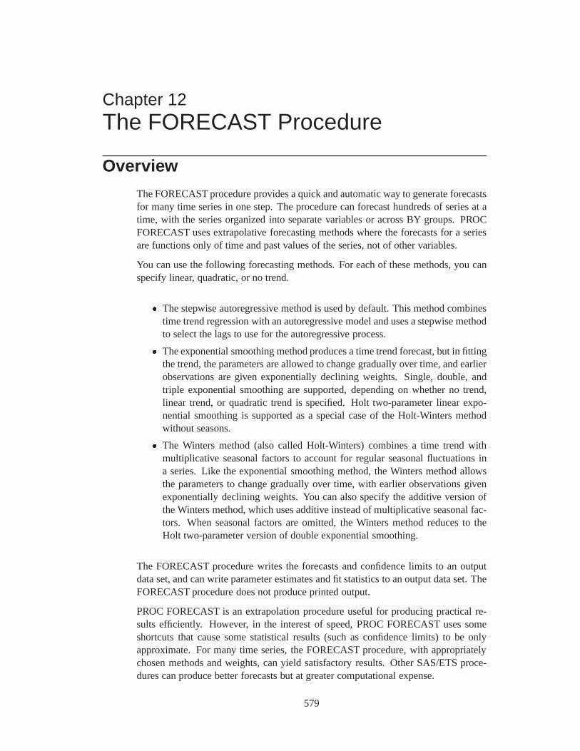
Overview
The FORECAST procedure provides a quick and automatic way to generate forecastsfor many time series in one step. The procedure can forecast hundreds of series at atime, with the series organized into separate variables or across BY groups. PROCFORECAST uses extrapolative forecasting methods where the forecasts for a seriesare functions only of time and past values of the series, not of other variables.
You can use the following forecasting methods. For each of these methods, you canspecify linear, quadratic, or no trend.
� The stepwise autoregressive method is used by default. This method combinestime trend regression with an autoregressive model and uses a stepwise methodto select the lags to use for the autoregressive process.
� The exponential smoothing method produces a time trend forecast, but in fittingthe trend, the parameters are allowed to change gradually over time, and earlierobservations are given exponentially declining weights. Single, double, andtriple exponential smoothing are supported, depending on whether no trend,linear trend, or quadratic trend is specified. Holt two-parameter linear expo-nential smoothing is supported as a special case of the Holt-Winters methodwithout seasons.
� The Winters method (also called Holt-Winters) combines a time trend withmultiplicative seasonal factors to account for regular seasonal fluctuations ina series. Like the exponential smoothing method, the Winters method allowsthe parameters to change gradually over time, with earlier observations givenexponentially declining weights. You can also specify the additive version ofthe Winters method, which uses additive instead of multiplicative seasonal fac-tors. When seasonal factors are omitted, the Winters method reduces to theHolt two-parameter version of double exponential smoothing.
The FORECAST procedure writes the forecasts and confidence limits to an outputdata set, and can write parameter estimates and fit statistics to an output data set. TheFORECAST procedure does not produce printed output.
PROC FORECAST is an extrapolation procedure useful for producing practical re-sults efficiently. However, in the interest of speed, PROC FORECAST uses someshortcuts that cause some statistical results (such as confidence limits) to be onlyapproximate. For many time series, the FORECAST procedure, with appropriatelychosen methods and weights, can yield satisfactory results. Other SAS/ETS proce-dures can produce better forecasts but at greater computational expense.
579
Part 2. General Information
You can perform the stepwise autoregressive forecasting method with the AUTOREGprocedure. You can perform exponential smoothing with statistically optimal weightsas an ARIMA model using the ARIMA procedure. Seasonal ARIMA models canbe used for forecasting seasonal series for which the Winters and additive Wintersmethods might be used.
Additionally, the Time Series Forecasting System can be used to develop forecastingmodels, estimate the model parameters, evaluate the models’ ability to forecast anddisplay the results graphically. See Chapter 23, “Getting Started with Time SeriesForecasting,” for more details.
SAS OnlineDoc: Version 8580
Chapter 12. Getting Started
Getting Started
To use PROC FORECAST, specify the input and output data sets and the numberof periods to forecast in the PROC FORECAST statement, then list the variables toforecast in a VAR statement.
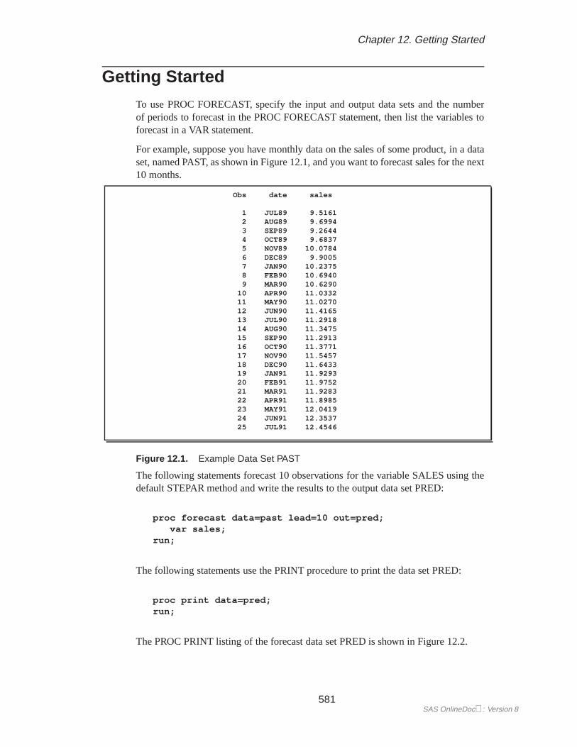
For example, suppose you have monthly data on the sales of some product, in a dataset, named PAST, as shown in Figure 12.1, and you want to forecast sales for the next10 months.
Obs date sales
1 JUL89 9.51612 AUG89 9.69943 SEP89 9.26444 OCT89 9.68375 NOV89 10.07846 DEC89 9.90057 JAN90 10.23758 FEB90 10.69409 MAR90 10.6290
10 APR90 11.033211 MAY90 11.027012 JUN90 11.416513 JUL90 11.291814 AUG90 11.347515 SEP90 11.291316 OCT90 11.377117 NOV90 11.545718 DEC90 11.643319 JAN91 11.929320 FEB91 11.975221 MAR91 11.928322 APR91 11.898523 MAY91 12.041924 JUN91 12.353725 JUL91 12.4546
Figure 12.1. Example Data Set PAST
The following statements forecast 10 observations for the variable SALES using thedefault STEPAR method and write the results to the output data set PRED:
proc forecast data=past lead=10 out=pred;var sales;
run;
The following statements use the PRINT procedure to print the data set PRED:
proc print data=pred;run;
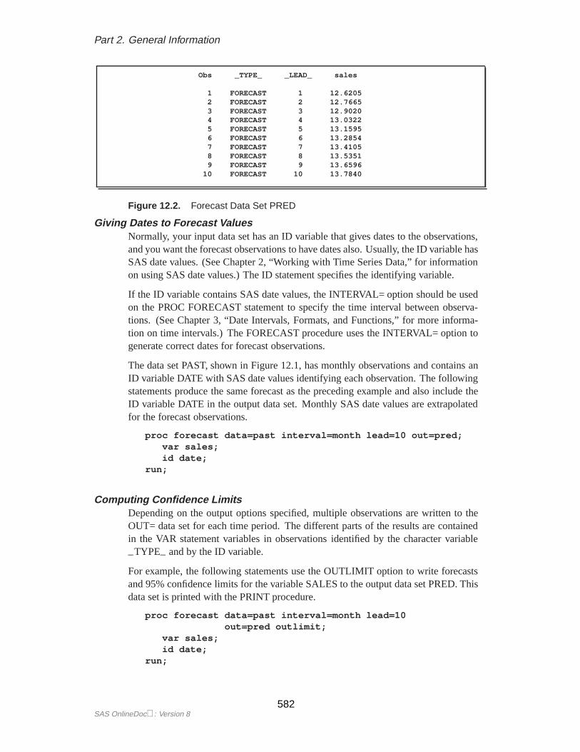
The PROC PRINT listing of the forecast data set PRED is shown in Figure 12.2.
581SAS OnlineDoc: Version 8
Part 2. General Information
Obs _TYPE_ _LEAD_ sales
1 FORECAST 1 12.62052 FORECAST 2 12.76653 FORECAST 3 12.90204 FORECAST 4 13.03225 FORECAST 5 13.15956 FORECAST 6 13.28547 FORECAST 7 13.41058 FORECAST 8 13.53519 FORECAST 9 13.6596
10 FORECAST 10 13.7840
Figure 12.2. Forecast Data Set PRED
Giving Dates to Forecast ValuesNormally, your input data set has an ID variable that gives dates to the observations,and you want the forecast observations to have dates also. Usually, the ID variable hasSAS date values. (See Chapter 2, “Working with Time Series Data,” for informationon using SAS date values.) The ID statement specifies the identifying variable.
If the ID variable contains SAS date values, the INTERVAL= option should be usedon the PROC FORECAST statement to specify the time interval between observa-tions. (See Chapter 3, “Date Intervals, Formats, and Functions,” for more informa-tion on time intervals.) The FORECAST procedure uses the INTERVAL= option togenerate correct dates for forecast observations.
The data set PAST, shown in Figure 12.1, has monthly observations and contains anID variable DATE with SAS date values identifying each observation. The followingstatements produce the same forecast as the preceding example and also include theID variable DATE in the output data set. Monthly SAS date values are extrapolatedfor the forecast observations.
proc forecast data=past interval=month lead=10 out=pred;var sales;id date;
run;
Computing Confidence LimitsDepending on the output options specified, multiple observations are written to theOUT= data set for each time period. The different parts of the results are containedin the VAR statement variables in observations identified by the character variable
–TYPE– and by the ID variable.
For example, the following statements use the OUTLIMIT option to write forecastsand 95% confidence limits for the variable SALES to the output data set PRED. Thisdata set is printed with the PRINT procedure.
proc forecast data=past interval=month lead=10out=pred outlimit;
var sales;id date;
run;
SAS OnlineDoc: Version 8582
Chapter 12. Getting Started
proc print data=pred;run;
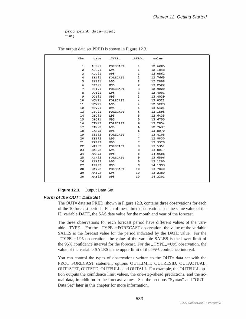
The output data set PRED is shown in Figure 12.3.
Obs date _TYPE_ _LEAD_ sales
1 AUG91 FORECAST 1 12.62052 AUG91 L95 1 12.18483 AUG91 U95 1 13.05624 SEP91 FORECAST 2 12.76655 SEP91 L95 2 12.28086 SEP91 U95 2 13.25227 OCT91 FORECAST 3 12.90208 OCT91 L95 3 12.40019 OCT91 U95 3 13.4039
10 NOV91 FORECAST 4 13.032211 NOV91 L95 4 12.522312 NOV91 U95 4 13.542113 DEC91 FORECAST 5 13.159514 DEC91 L95 5 12.643515 DEC91 U95 5 13.675516 JAN92 FORECAST 6 13.285417 JAN92 L95 6 12.763718 JAN92 U95 6 13.807019 FEB92 FORECAST 7 13.410520 FEB92 L95 7 12.883021 FEB92 U95 7 13.937922 MAR92 FORECAST 8 13.535123 MAR92 L95 8 13.001724 MAR92 U95 8 14.068625 APR92 FORECAST 9 13.659626 APR92 L95 9 13.120027 APR92 U95 9 14.199328 MAY92 FORECAST 10 13.784029 MAY92 L95 10 13.238030 MAY92 U95 10 14.3301
Figure 12.3. Output Data Set
Form of the OUT= Data SetThe OUT= data set PRED, shown in Figure 12.3, contains three observations for eachof the 10 forecast periods. Each of these three observations has the same value of theID variable DATE, the SAS date value for the month and year of the forecast.
The three observations for each forecast period have different values of the vari-able–TYPE–. For the–TYPE–=FORECAST observation, the value of the variableSALES is the forecast value for the period indicated by the DATE value. For the
–TYPE–=L95 observation, the value of the variable SALES is the lower limit ofthe 95% confidence interval for the forecast. For the–TYPE–=U95 observation, thevalue of the variable SALES is the upper limit of the 95% confidence interval.
You can control the types of observations written to the OUT= data set with thePROC FORECAST statement options OUTLIMIT, OUTRESID, OUTACTUAL,OUT1STEP, OUTSTD, OUTFULL, and OUTALL. For example, the OUTFULL op-tion outputs the confidence limit values, the one-step-ahead predictions, and the ac-tual data, in addition to the forecast values. See the sections "Syntax" and "OUT=Data Set" later in this chapter for more information.
583SAS OnlineDoc: Version 8
Part 2. General Information
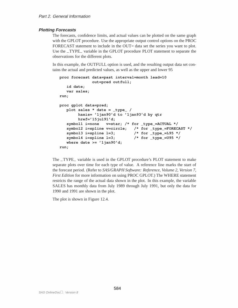
Plotting ForecastsThe forecasts, confidence limits, and actual values can be plotted on the same graphwith the GPLOT procedure. Use the appropriate output control options on the PROCFORECAST statement to include in the OUT= data set the series you want to plot.Use the–TYPE– variable in the GPLOT procedure PLOT statement to separate theobservations for the different plots.
In this example, the OUTFULL option is used, and the resulting output data set con-tains the actual and predicted values, as well as the upper and lower 95
proc forecast data=past interval=month lead=10out=pred outfull;
id date;var sales;
run;
proc gplot data=pred;plot sales * date = _type_ /
haxis= ’1jan90’d to ’1jan93’d by qtrhref=’15jul91’d;
symbol1 i=none v=star; /* for _type_=ACTUAL */symbol2 i=spline v=circle; /* for _type_=FORECAST */symbol3 i=spline l=3; /* for _type_=L95 */symbol4 i=spline l=3; /* for _type_=U95 */where date >= ’1jan90’d;
run;
The –TYPE– variable is used in the GPLOT procedure’s PLOT statement to makeseparate plots over time for each type of value. A reference line marks the start ofthe forecast period. (Refer toSAS/GRAPH Software: Reference, Volume 2, Version 7,First Edition for more information on using PROC GPLOT.) The WHERE statementrestricts the range of the actual data shown in the plot. In this example, the variableSALES has monthly data from July 1989 through July 1991, but only the data for1990 and 1991 are shown in the plot.
The plot is shown in Figure 12.4.
SAS OnlineDoc: Version 8584
Chapter 12. Getting Started
Figure 12.4. Plot of Forecast with Confidence Limits
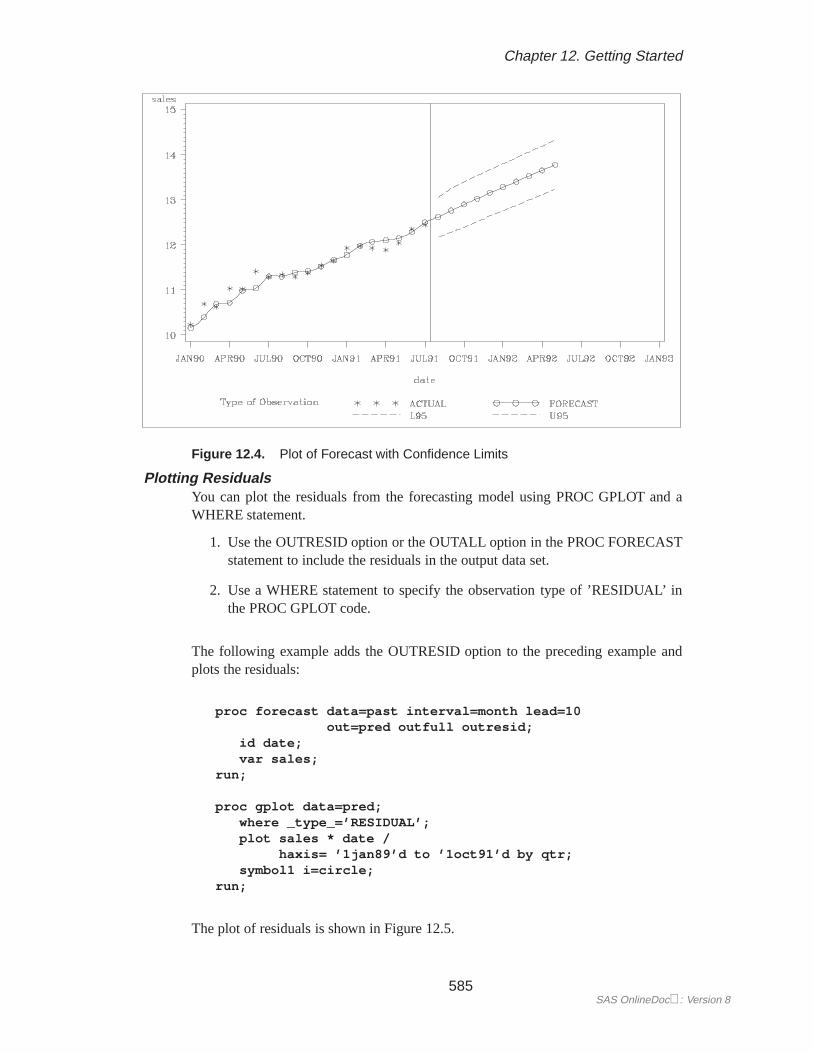
Plotting ResidualsYou can plot the residuals from the forecasting model using PROC GPLOT and aWHERE statement.
1. Use the OUTRESID option or the OUTALL option in the PROC FORECASTstatement to include the residuals in the output data set.
2. Use a WHERE statement to specify the observation type of ’RESIDUAL’ inthe PROC GPLOT code.
The following example adds the OUTRESID option to the preceding example andplots the residuals:
proc forecast data=past interval=month lead=10out=pred outfull outresid;
id date;var sales;
run;
proc gplot data=pred;where _type_=’RESIDUAL’;plot sales * date /
haxis= ’1jan89’d to ’1oct91’d by qtr;symbol1 i=circle;
run;
The plot of residuals is shown in Figure 12.5.
585SAS OnlineDoc: Version 8
Part 2. General Information
Figure 12.5. Plot of Residuals
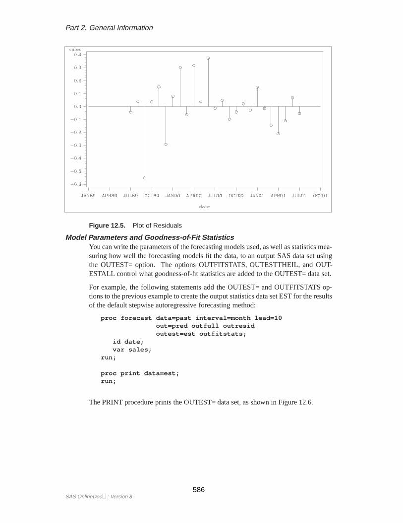
Model Parameters and Goodness-of-Fit StatisticsYou can write the parameters of the forecasting models used, as well as statistics mea-suring how well the forecasting models fit the data, to an output SAS data set usingthe OUTEST= option. The options OUTFITSTATS, OUTESTTHEIL, and OUT-ESTALL control what goodness-of-fit statistics are added to the OUTEST= data set.
For example, the following statements add the OUTEST= and OUTFITSTATS op-tions to the previous example to create the output statistics data set EST for the resultsof the default stepwise autoregressive forecasting method:
proc forecast data=past interval=month lead=10out=pred outfull outresidoutest=est outfitstats;
id date;var sales;
run;
proc print data=est;run;
The PRINT procedure prints the OUTEST= data set, as shown in Figure 12.6.
SAS OnlineDoc: Version 8586
Chapter 12. Getting Started
Obs _TYPE_ date sales
1 N JUL91 252 NRESID JUL91 253 DF JUL91 224 SIGMA JUL91 0.20016135 CONSTANT JUL91 9.43488226 LINEAR JUL91 0.12426487 AR1 JUL91 0.52062948 AR2 JUL91 .9 AR3 JUL91 .
10 AR4 JUL91 .11 AR5 JUL91 .12 AR6 JUL91 .13 AR7 JUL91 .14 AR8 JUL91 .15 SST JUL91 21.2834216 SSE JUL91 0.879371417 MSE JUL91 0.039971418 RMSE JUL91 0.199928619 MAPE JUL91 1.228008920 MPE JUL91 -0.05013921 MAE JUL91 0.131211522 ME JUL91 -0.00181123 MAXE JUL91 0.373232824 MINE JUL91 -0.55160525 MAXPE JUL91 3.269229426 MINPE JUL91 -5.95402227 RSQUARE JUL91 0.958682828 ADJRSQ JUL91 0.954926729 RW_RSQ JUL91 0.265780130 ARSQ JUL91 0.947414531 APC JUL91 0.04476832 AIC JUL91 -77.6855933 SBC JUL91 -74.0289734 CORR JUL91 0.9791313
Figure 12.6. The OUTEST= Data Set for STEPAR Method
In the OUTEST= data set, the DATE variable contains the ID value of the last ob-servation in the data set used to fit the forecasting model. The variable SALES con-tains the statistic indicated by the value of the–TYPE– variable. The–TYPE–=N,NRESID, and DF observations contain, respectively, the number of observations readfrom the data set, the number of nonmissing residuals used to compute the goodness-of-fit statistics, and the number of nonmissing observations minus the number ofparameters used in the forecasting model.
The observation having–TYPE–=SIGMA contains the estimate of the standarddeviation of the one-step prediction error computed from the residuals. The
–TYPE–=CONSTANT and–TYPE–=LINEAR contain the coefficients of the timetrend regression. The–TYPE–=AR1, AR2, ..., AR8 observations contain the esti-mated autoregressive parameters. A missing autoregressive parameter indicates thatthe autoregressive term at that lag was not included in the model by the stepwisemodel selection method. (See the section "STEPAR Method" later in this chapter formore information.)
The other observations in the OUTEST= data set contain various goodness-of-fitstatistics that measure how well the forecasting model used fits the given data. See"OUTEST= Data Set" later in this chapter for details.
587SAS OnlineDoc: Version 8
Part 2. General Information
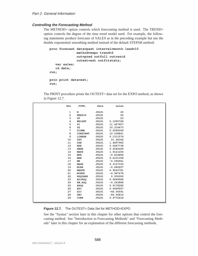
Controlling the Forecasting MethodThe METHOD= option controls which forecasting method is used. The TREND=option controls the degree of the time trend model used. For example, the follow-ing statements produce forecasts of SALES as in the preceding example but use thedouble exponential smoothing method instead of the default STEPAR method:
proc forecast data=past interval=month lead=10method=expo trend=2out=pred outfull outresidoutest=est outfitstats;
var sales;id date;
run;
proc print data=est;run;
The PRINT procedure prints the OUTEST= data set for the EXPO method, as shownin Figure 12.7.
Obs _TYPE_ date sales
1 N JUL91 252 NRESID JUL91 253 DF JUL91 234 WEIGHT JUL91 0.10557285 S1 JUL91 11.4276576 S2 JUL91 10.3164737 SIGMA JUL91 0.25450698 CONSTANT JUL91 12.5388419 LINEAR JUL91 0.1311574
10 SST JUL91 21.2834211 SSE JUL91 1.489796512 MSE JUL91 0.064773813 RMSE JUL91 0.254506914 MAPE JUL91 1.912120415 MPE JUL91 -0.81688616 MAE JUL91 0.210135817 ME JUL91 -0.09494118 MAXE JUL91 0.312733219 MINE JUL91 -0.46020720 MAXPE JUL91 2.924378121 MINPE JUL91 -4.96747822 RSQUARE JUL91 0.93000223 ADJRSQ JUL91 0.926958624 RW_RSQ JUL91 -0.24388625 ARSQ JUL91 0.917828526 APC JUL91 0.069955727 AIC JUL91 -66.5059128 SBC JUL91 -64.0681629 CORR JUL91 0.9772418
Figure 12.7. The OUTEST= Data Set for METHOD=EXPO
See the "Syntax" section later in this chapter for other options that control the fore-casting method. See "Introduction to Forecasting Methods" and "Forecasting Meth-ods" later in this chapter for an explanation of the different forecasting methods.
SAS OnlineDoc: Version 8588
Chapter 12. Getting Started
Introduction to Forecasting Methods
This section briefly introduces the forecasting methods used by the FORECAST pro-cedure. Refer to textbooks on forecasting and see "Forecasting Methods" later in thischapter for more detailed discussions of forecasting methods.
The FORECAST procedure combines three basic models to fit time series:
� time trend models for long-term, deterministic change
� autoregressive models for short-term fluctuations
� seasonal models for regular seasonal fluctuations
Two approaches to time series modeling and forecasting aretime trend modelsandtime series methods.
Time Trend ModelsTime trend models assume that there is some permanent deterministic pattern acrosstime. These models are best suited to data that are not dominated by random fluctua-tions.
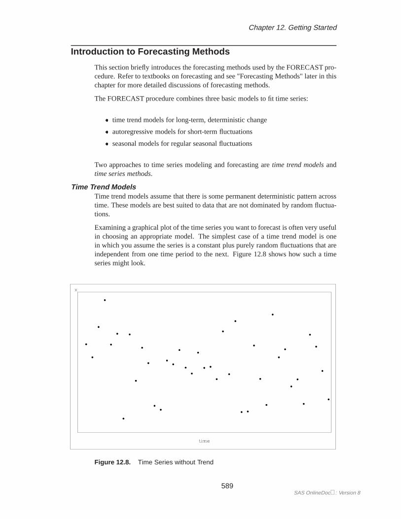
Examining a graphical plot of the time series you want to forecast is often very usefulin choosing an appropriate model. The simplest case of a time trend model is onein which you assume the series is a constant plus purely random fluctuations that areindependent from one time period to the next. Figure 12.8 shows how such a timeseries might look.
Figure 12.8. Time Series without Trend
589SAS OnlineDoc: Version 8
Part 2. General Information
Thex t values are generated according to the equation
xt = b0 + �t
where�t is an independent, zero-mean, random error, andb0 is the true series mean.
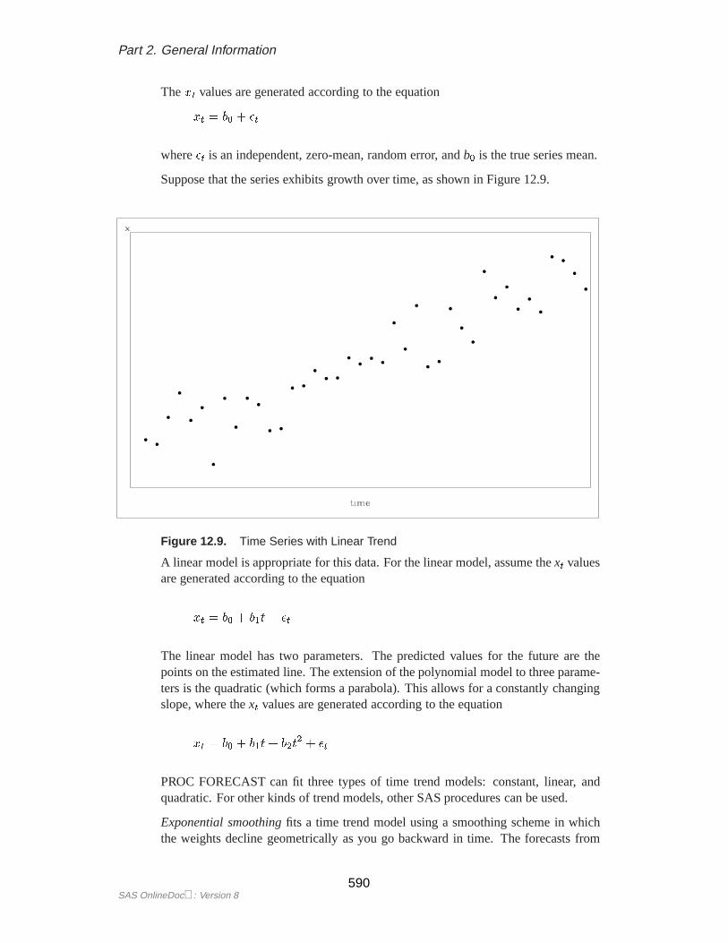
Suppose that the series exhibits growth over time, as shown in Figure 12.9.
Figure 12.9. Time Series with Linear Trend
A linear model is appropriate for this data. For the linear model, assume thext valuesare generated according to the equation
xt = b0 + b1t+ �t
The linear model has two parameters. The predicted values for the future are thepoints on the estimated line. The extension of the polynomial model to three parame-ters is the quadratic (which forms a parabola). This allows for a constantly changingslope, where thext values are generated according to the equation
xt = b0 + b1t+ b2t2 + �t
PROC FORECAST can fit three types of time trend models: constant, linear, andquadratic. For other kinds of trend models, other SAS procedures can be used.
Exponential smoothingfits a time trend model using a smoothing scheme in whichthe weights decline geometrically as you go backward in time. The forecasts from
SAS OnlineDoc: Version 8590
Chapter 12. Getting Started
exponential smoothing are a time trend, but the trend is based mostly on the recent ob-servations instead of on all the observations equally. How well exponential smoothingworks as a forecasting method depends on choosing a good smoothing weight for theseries.
To specify the exponential smoothing method, use the METHOD=EXPO option. Sin-gle exponential smoothing produces forecasts with a constant trend (that is, no trend).Double exponential smoothing produces forecasts with a linear trend, and triple ex-ponential smoothing produces a quadratic trend. Use the TREND= option with theMETHOD=EXPO option to select single, double, or triple exponential smoothing.
The time trend model can be modified to account for regular seasonal fluctuations ofthe series about the trend. To capture seasonality, the trend model includes a seasonalparameter for each season. Seasonal models can be additive or multiplicative.
xt = b0 + b1t+ s(t) + �t (Additive)
xt = (b0 + b1t)s(t) + �t (Multiplicative)
wheres(t) is the seasonal parameter for the season corresponding to timet.
The Winters method is similar to exponential smoothing, but includes seasonal fac-tors. The Winters method can use either additive or multiplicative seasonal factors.Like exponential smoothing, good results with the Winters method depend on choos-ing good smoothing weights for the series to be forecast.
To specify the multiplicative or additive versions of the Winters method, use theMETHOD=WINTERS or METHOD=ADDWINTERS options, respectively. Tospecify seasonal factors to include in the model, use the SEASONS= option.
Many observed time series do not behave like constant, linear, or quadratic timetrends. However, you can partially compensate for the inadequacies of the trend mod-els by fitting time series models to the departures from the time trend, as described inthe following sections.
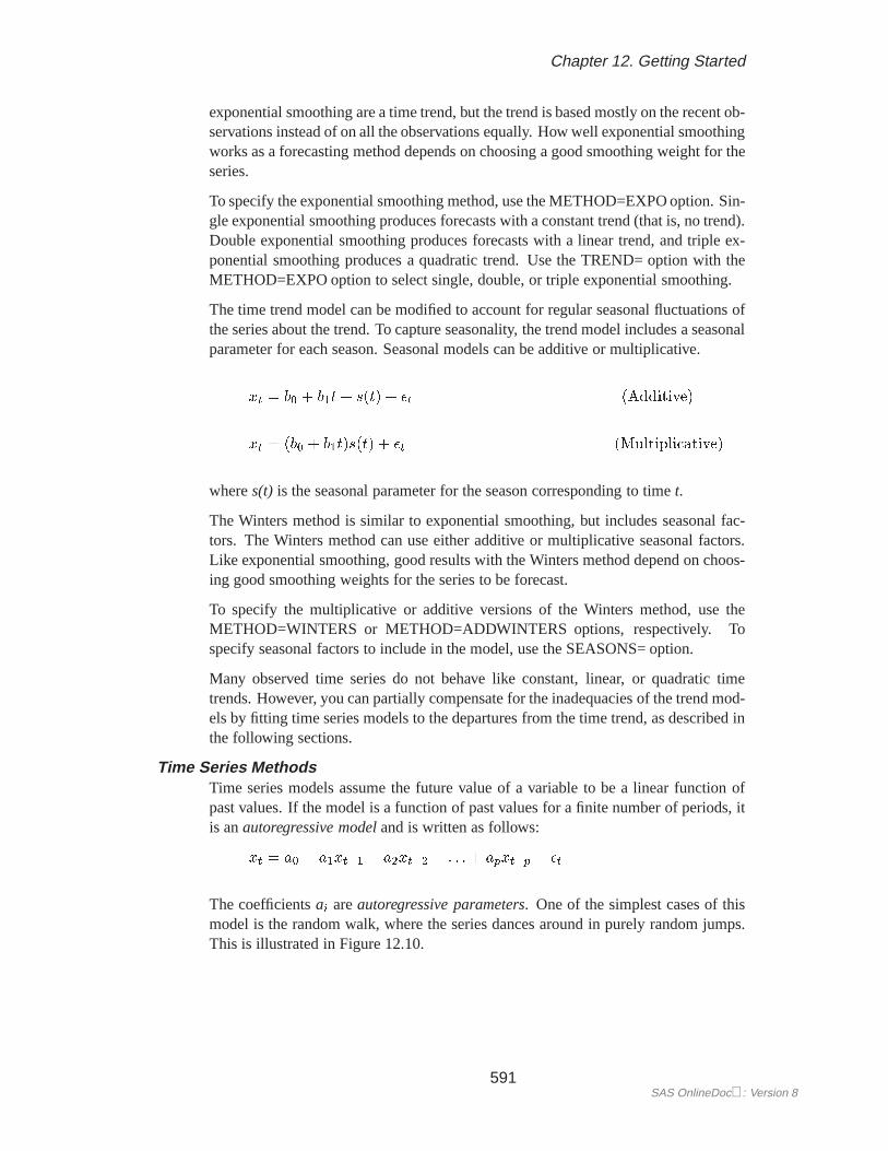
Time Series MethodsTime series models assume the future value of a variable to be a linear function ofpast values. If the model is a function of past values for a finite number of periods, itis anautoregressive modeland is written as follows:
xt = a0 + a1xt�1 + a2xt�2 + : : : + apxt�p + �t
The coefficientsai areautoregressive parameters. One of the simplest cases of thismodel is the random walk, where the series dances around in purely random jumps.This is illustrated in Figure 12.10.
591SAS OnlineDoc: Version 8

Part 2. General Information
Figure 12.10. Random Walk Series
Thext values are generated by the equation
xt = xt�1 + �t
In this type of model, the best forecast of a future value is the present value. However,with other autoregressive models, the best forecast is a weighted sum of recent values.Pure autoregressive forecasts always damp down to a constant (assuming the processis stationary).
Autoregressive time series models can also be used to predict seasonal fluctuations.
Combining Time Trend with Autoregressive ModelsTrend models are suitable for capturing long-term behavior, whereas autoregressivemodels are more appropriate for capturing short-term fluctuations. One approach toforecasting is to combine a deterministic time trend model with an autoregressivemodel.
The stepwise autoregressive method(STEPAR method) combines a time-trend re-gression with an autoregressive model for departures from trend. The combinedtime-trend and autoregressive model is written as follows:
xt = b0 + b1t+ b2t2 + ut
ut = a1ut�1 + a2ut�2 + : : :+ aput�p + �t
The autoregressive parameters included in the model for each series are selected by astepwise regression procedure, so that autoregressive parameters are only included atthose lags at which they are statistically significant.
SAS OnlineDoc: Version 8592

Chapter 12. Getting Started
The stepwise autoregressive method is fully automatic and, unlike the exponentialsmoothing and Winters methods, does not depend on choosing smoothing weights.However, the STEPAR method assumes that the long-term trend is stable; that is, thetime trend regression is fit to the whole series with equal weights for the observations.
The stepwise autoregressive model is used when you specify the METHOD=STEPARoption or do not specify any METHOD= option. To select a constant, linear, orquadratic trend for the time-trend part of the model, use the TREND= option.
593SAS OnlineDoc: Version 8
Part 2. General Information
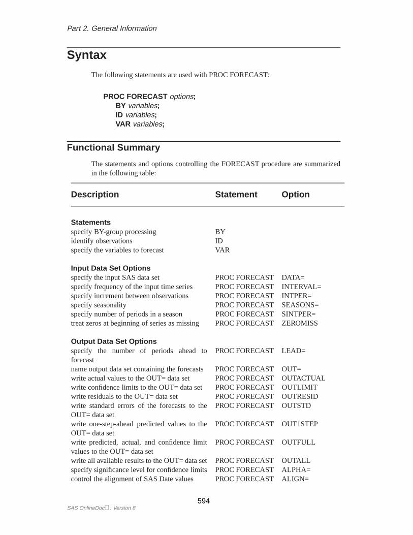
Syntax
The following statements are used with PROC FORECAST:
PROC FORECAST options;BY variables;ID variables;VAR variables;
Functional Summary
The statements and options controlling the FORECAST procedure are summarizedin the following table:
Description Statement Option
Statementsspecify BY-group processing BYidentify observations IDspecify the variables to forecast VAR
Input Data Set Optionsspecify the input SAS data set PROC FORECAST DATA=specify frequency of the input time series PROC FORECAST INTERVAL=specify increment between observations PROC FORECAST INTPER=specify seasonality PROC FORECAST SEASONS=specify number of periods in a season PROC FORECAST SINTPER=treat zeros at beginning of series as missing PROC FORECAST ZEROMISS
Output Data Set Optionsspecify the number of periods ahead toforecast
PROC FORECAST LEAD=
name output data set containing the forecasts PROC FORECAST OUT=write actual values to the OUT= data set PROC FORECAST OUTACTUALwrite confidence limits to the OUT= data set PROC FORECAST OUTLIMITwrite residuals to the OUT= data set PROC FORECAST OUTRESIDwrite standard errors of the forecasts to theOUT= data set
PROC FORECAST OUTSTD
write one-step-ahead predicted values to theOUT= data set
PROC FORECAST OUT1STEP
write predicted, actual, and confidence limitvalues to the OUT= data set
PROC FORECAST OUTFULL
write all available results to the OUT= data set PROC FORECAST OUTALLspecify significance level for confidence limits PROC FORECAST ALPHA=control the alignment of SAS Date values PROC FORECAST ALIGN=
SAS OnlineDoc: Version 8594
Chapter 12. Syntax
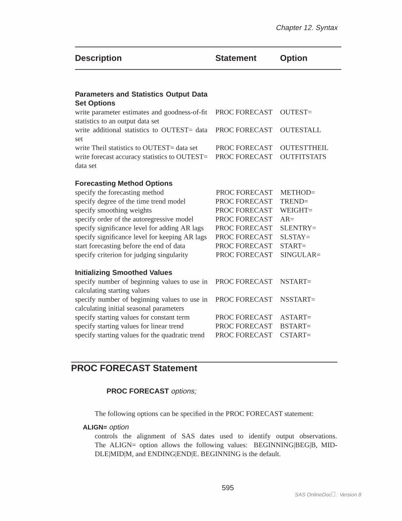
Description Statement Option
Parameters and Statistics Output DataSet Optionswrite parameter estimates and goodness-of-fitstatistics to an output data set
PROC FORECAST OUTEST=
write additional statistics to OUTEST= dataset
PROC FORECAST OUTESTALL
write Theil statistics to OUTEST= data set PROC FORECAST OUTESTTHEILwrite forecast accuracy statistics to OUTEST=data set
PROC FORECAST OUTFITSTATS
Forecasting Method Optionsspecify the forecasting method PROC FORECAST METHOD=specify degree of the time trend model PROC FORECAST TREND=specify smoothing weights PROC FORECAST WEIGHT=specify order of the autoregressive model PROC FORECAST AR=specify significance level for adding AR lags PROC FORECAST SLENTRY=specify significance level for keeping AR lags PROC FORECAST SLSTAY=start forecasting before the end of data PROC FORECAST START=specify criterion for judging singularity PROC FORECAST SINGULAR=
Initializing Smoothed Valuesspecify number of beginning values to use incalculating starting values
PROC FORECAST NSTART=
specify number of beginning values to use incalculating initial seasonal parameters
PROC FORECAST NSSTART=
specify starting values for constant term PROC FORECAST ASTART=specify starting values for linear trend PROC FORECAST BSTART=specify starting values for the quadratic trend PROC FORECAST CSTART=
PROC FORECAST Statement
PROC FORECAST options;
The following options can be specified in the PROC FORECAST statement:
ALIGN= optioncontrols the alignment of SAS dates used to identify output observations.The ALIGN= option allows the following values: BEGINNING|BEG|B, MID-DLE|MID|M, and ENDING|END|E. BEGINNING is the default.
595SAS OnlineDoc: Version 8
Part 2. General Information
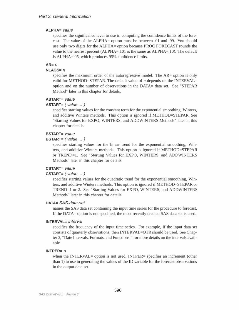
ALPHA= valuespecifies the significance level to use in computing the confidence limits of the fore-cast. The value of the ALPHA= option must be between .01 and .99. You shoulduse only two digits for the ALPHA= option because PROC FORECAST rounds thevalue to the nearest percent (ALPHA=.101 is the same as ALPHA=.10). The defaultis ALPHA=.05, which produces 95% confidence limits.
AR= nNLAGS= n
specifies the maximum order of the autoregressive model. The AR= option is onlyvalid for METHOD=STEPAR. The default value ofn depends on the INTERVAL=option and on the number of observations in the DATA= data set. See "STEPARMethod" later in this chapter for details.
ASTART= valueASTART= ( value ... )
specifies starting values for the constant term for the exponential smoothing, Winters,and additive Winters methods. This option is ignored if METHOD=STEPAR. See"Starting Values for EXPO, WINTERS, and ADDWINTERS Methods" later in thischapter for details.
BSTART= valueBSTART= ( value ... )
specifies starting values for the linear trend for the exponential smoothing, Win-ters, and additive Winters methods. This option is ignored if METHOD=STEPARor TREND=1. See "Starting Values for EXPO, WINTERS, and ADDWINTERSMethods" later in this chapter for details.
CSTART= valueCSTART= ( value ... )
specifies starting values for the quadratic trend for the exponential smoothing, Win-ters, and additive Winters methods. This option is ignored if METHOD=STEPAR orTREND=1 or 2. See "Starting Values for EXPO, WINTERS, and ADDWINTERSMethods" later in this chapter for details.
DATA= SAS-data-setnames the SAS data set containing the input time series for the procedure to forecast.If the DATA= option is not specified, the most recently created SAS data set is used.
INTERVAL= intervalspecifies the frequency of the input time series. For example, if the input data setconsists of quarterly observations, then INTERVAL=QTR should be used. See Chap-ter 3, “Date Intervals, Formats, and Functions,” for more details on the intervals avail-able.
INTPER= nwhen the INTERVAL= option is not used, INTPER= specifies an increment (otherthan 1) to use in generating the values of the ID variable for the forecast observationsin the output data set.
SAS OnlineDoc: Version 8596
Chapter 12. Syntax
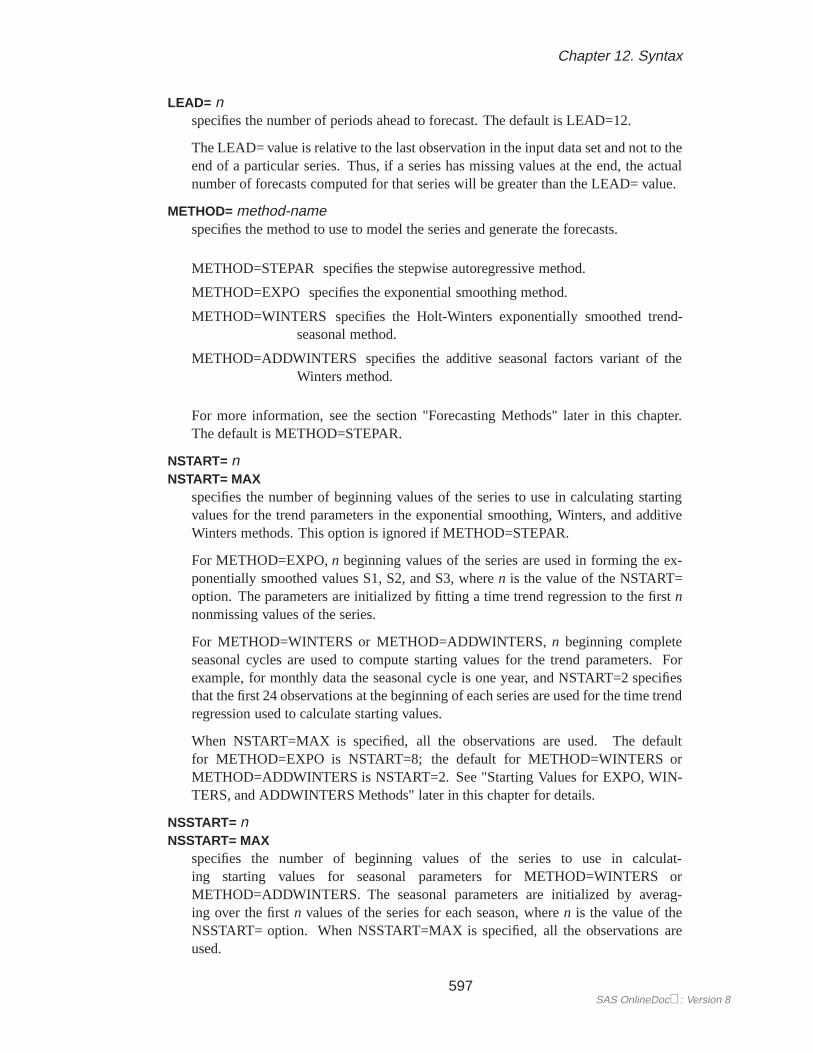
LEAD= nspecifies the number of periods ahead to forecast. The default is LEAD=12.
The LEAD= value is relative to the last observation in the input data set and not to theend of a particular series. Thus, if a series has missing values at the end, the actualnumber of forecasts computed for that series will be greater than the LEAD= value.
METHOD= method-namespecifies the method to use to model the series and generate the forecasts.
METHOD=STEPAR specifies the stepwise autoregressive method.
METHOD=EXPO specifies the exponential smoothing method.
METHOD=WINTERS specifies the Holt-Winters exponentially smoothed trend-seasonal method.
METHOD=ADDWINTERS specifies the additive seasonal factors variant of theWinters method.
For more information, see the section "Forecasting Methods" later in this chapter.The default is METHOD=STEPAR.
NSTART= nNSTART= MAX
specifies the number of beginning values of the series to use in calculating startingvalues for the trend parameters in the exponential smoothing, Winters, and additiveWinters methods. This option is ignored if METHOD=STEPAR.
For METHOD=EXPO,n beginning values of the series are used in forming the ex-ponentially smoothed values S1, S2, and S3, wheren is the value of the NSTART=option. The parameters are initialized by fitting a time trend regression to the firstnnonmissing values of the series.
For METHOD=WINTERS or METHOD=ADDWINTERS,n beginning completeseasonal cycles are used to compute starting values for the trend parameters. Forexample, for monthly data the seasonal cycle is one year, and NSTART=2 specifiesthat the first 24 observations at the beginning of each series are used for the time trendregression used to calculate starting values.
When NSTART=MAX is specified, all the observations are used. The defaultfor METHOD=EXPO is NSTART=8; the default for METHOD=WINTERS orMETHOD=ADDWINTERS is NSTART=2. See "Starting Values for EXPO, WIN-TERS, and ADDWINTERS Methods" later in this chapter for details.
NSSTART= nNSSTART= MAX
specifies the number of beginning values of the series to use in calculat-ing starting values for seasonal parameters for METHOD=WINTERS orMETHOD=ADDWINTERS. The seasonal parameters are initialized by averag-ing over the firstn values of the series for each season, wheren is the value of theNSSTART= option. When NSSTART=MAX is specified, all the observations areused.
597SAS OnlineDoc: Version 8
Part 2. General Information
If NSTART= is specified, but NSSTART= is not, NSSTART= defaults to the valuespecified for NSTART=. If neither NSTART= nor NSSTART= is specified, thenthe default is NSSTART=2. This option is ignored if METHOD=STEPAR orMETHOD=EXPO. See "Starting Values for EXPO, WINTERS, and ADDWINTERSMethods" later in this chapter for details.
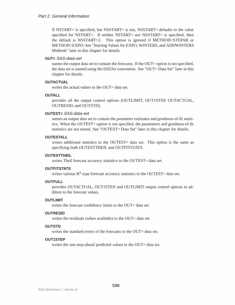
OUT= SAS-data-setnames the output data set to contain the forecasts. If the OUT= option is not specified,the data set is named using the DATAn convention. See "OUT= Data Set" later in thischapter for details.
OUTACTUALwrites the actual values to the OUT= data set.
OUTALLprovides all the output control options (OUTLIMIT, OUT1STEP, OUTACTUAL,OUTRESID, and OUTSTD).
OUTEST= SAS-data-setnames an output data set to contain the parameter estimates and goodness-of-fit statis-tics. When the OUTEST= option is not specified, the parameters and goodness-of-fitstatistics are not stored. See "OUTEST= Data Set" later in this chapter for details.
OUTESTALLwrites additional statistics to the OUTEST= data set. This option is the same asspecifying both OUTESTTHEIL and OUTFITSTATS.
OUTESTTHEILwrites Theil forecast accuracy statistics to the OUTEST= data set.
OUTFITSTATSwrites various R2-type forecast accuracy statistics to the OUTEST= data set.
OUTFULLprovides OUTACTUAL, OUT1STEP, and OUTLIMIT output control options in ad-dition to the forecast values.
OUTLIMITwrites the forecast confidence limits to the OUT= data set.
OUTRESIDwrites the residuals (when available) to the OUT= data set.
OUTSTDwrites the standard errors of the forecasts to the OUT= data set.
OUT1STEPwrites the one-step-ahead predicted values to the OUT= data set.
SAS OnlineDoc: Version 8598
Chapter 12. Syntax
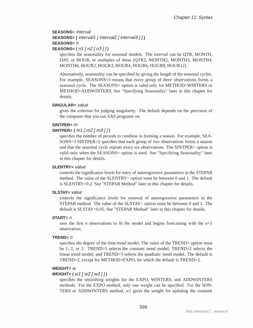
SEASONS= intervalSEASONS= ( interval1 [ interval2 [ interval3 ] ] )SEASONS= nSEASONS= ( n1 [ n2 [ n3 ] ] )
specifies the seasonality for seasonal models. Theinterval can be QTR, MONTH,DAY, or HOUR, or multiples of these (QTR2, MONTH2, MONTH3, MONTH4,MONTH6, HOUR2, HOUR3, HOUR4, HOUR6, HOUR8, HOUR12).
Alternatively, seasonality can be specified by giving the length of the seasonal cycles.For example, SEASONS=3 means that every group of three observations forms aseasonal cycle. The SEASONS= option is valid only for METHOD=WINTERS orMETHOD=ADDWINTERS. See "Specifying Seasonality" later in this chapter fordetails.
SINGULAR= valuegives the criterion for judging singularity. The default depends on the precision ofthe computer that you run SAS programs on.
SINTPER= mSINTPER= ( m1 [ m2 [ m3 ] ] )
specifies the number of periods to combine in forming a season. For example, SEA-SONS=3 SINTPER=2 specifies that each group of two observations forms a seasonand that the seasonal cycle repeats every six observations. The SINTPER= option isvalid only when the SEASONS= option is used. See "Specifying Seasonality" laterin this chapter for details.
SLENTRY= valuecontrols the significance levels for entry of autoregressive parameters in the STEPARmethod. The value of the SLENTRY= option must be between 0 and 1. The defaultis SLENTRY=0.2. See "STEPAR Method" later in this chapter for details.
SLSTAY= valuecontrols the significance levels for removal of autoregressive parameters in theSTEPAR method. The value of the SLSTAY= option must be between 0 and 1. Thedefault is SLSTAY=0.05. See "STEPAR Method" later in this chapter for details.
START= nuses the firstn observations to fit the model and begins forecasting with then+1observation.
TREND= nspecifies the degree of the time trend model. The value of the TREND= option mustbe 1, 2, or 3. TREND=1 selects the constant trend model; TREND=2 selects thelinear trend model; and TREND=3 selects the quadratic trend model. The default isTREND=2, except for METHOD=EXPO, for which the default is TREND=3.
WEIGHT= wWEIGHT= ( w1 [ w2 [ w3 ] ] )
specifies the smoothing weights for the EXPO, WINTERS, and ADDWINTERSmethods. For the EXPO method, only one weight can be specified. For the WIN-TERS or ADDWINTERS method,w1 gives the weight for updating the constant
599SAS OnlineDoc: Version 8
Part 2. General Information
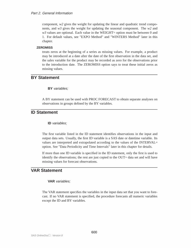
component,w2 gives the weight for updating the linear and quadratic trend compo-nents, andw3 gives the weight for updating the seasonal component. Thew2 andw3 values are optional. Each value in the WEIGHT= option must be between 0 and1. For default values, see "EXPO Method" and "WINTERS Method" later in thischapter.
ZEROMISStreats zeros at the beginning of a series as missing values. For example, a productmay be introduced at a date after the date of the first observation in the data set, andthe sales variable for the product may be recorded as zero for the observations priorto the introduction date. The ZEROMISS option says to treat these initial zeros asmissing values.
BY Statement
BY variables;
A BY statement can be used with PROC FORECAST to obtain separate analyses onobservations in groups defined by the BY variables.
ID Statement
ID variables;
The first variable listed in the ID statement identifies observations in the input andoutput data sets. Usually, the first ID variable is a SAS date or datetime variable. Itsvalues are interpreted and extrapolated according to the values of the INTERVAL=option. See "Data Periodicity and Time Intervals" later in this chapter for details.
If more than one ID variable is specified in the ID statement, only the first is used toidentify the observations; the rest are just copied to the OUT= data set and will havemissing values for forecast observations.
VAR Statement
VAR variables;
The VAR statement specifies the variables in the input data set that you want to fore-cast. If no VAR statement is specified, the procedure forecasts all numeric variablesexcept the ID and BY variables.
SAS OnlineDoc: Version 8600

Chapter 12. Details
Details
Missing Values
The treatment of missing values varies by method. For METHOD=STEPAR, missingvalues are tolerated in the series; the autocorrelations are estimated from the avail-able data and tapered, if necessary. For the EXPO, WINTERS, and ADDWINTERSmethods, missing values after the start of the series are replaced with one-step-aheadpredicted values, and the predicted values are applied to the smoothing equations.For the WINTERS method, negative or zero values are treated as missing.
Data Periodicity and Time Intervals
The INTERVAL= option is used to establish the frequency of the time series. Forexample, INTERVAL=MONTH specifies that each observation in the input data setrepresents one month. If INTERVAL=MONTH2, each observation represents twomonths. Thus, there is a two-month time interval between each pair of successiveobservations, and the data frequency is bimonthly.
See Chapter 3, “Date Intervals, Formats, and Functions,” for details on the intervalvalues supported.
The INTERVAL= option is used together with the ID statement to fully describethe observations that make up the time series. The first variable specified in the IDstatement is used to identify the observations. Usually, SAS date or datetime valuesare used for this variable. PROC FORECAST uses the ID variable in the followingways:
� to validate the data periodicity. When the INTERVAL= option is specified, theID variable is used to check the data and verify that successive observationshave valid ID values corresponding to successive time intervals. When theINTERVAL= option is not used, PROC FORECAST verifies that the ID valuesare nonmissing and in ascending order. A warning message is printed when aninvalid ID value is found in the input data set.
� to check for gaps in the input observations. For example, if INTER-VAL=MONTH and an input observation for January 1970 is followed by anobservation for April 1970, there is a gap in the input data, with two obser-vations omitted. When a gap in the input data is found, a warning messageis printed, and PROC FORECAST processes missing values for each omittedinput observation.
� to label the forecast observations in the output data set. The values of the IDvariable for the forecast observations after the end of the input data set areextrapolated according to the frequency specifications of the INTERVAL= op-tion. If the INTERVAL= option is not specified, the ID variable is extrapolatedby incrementing the ID variable value for the last observation in the input dataset by the INTPER= value, if specified, or by one.
601SAS OnlineDoc: Version 8

Part 2. General Information
The ALIGN= option controls the alignment of SAS dates. See Chapter 3, “DateIntervals, Formats, and Functions,” for more information.
Forecasting Methods
This section explains the forecasting methods used by PROC FORECAST.
STEPAR MethodIn the STEPAR method, PROC FORECAST first fits a time trend model to the seriesand takes the difference between each value and the estimated trend. (This process iscalleddetrending.) Then, the remaining variation is fit using an autoregressive model.
The STEPAR method fits the autoregressive process to the residuals of the trendmodel using a backwards-stepping method to select parameters. Since the trend andautoregressive parameters are fit in sequence rather than simultaneously, the parame-ter estimates are not optimal in a statistical sense; however, the estimates are usuallyclose to optimal, and the method is computationally inexpensive.
The STEPAR AlgorithmThe STEPAR method consists of the following computational steps:
1. Fit the trend model as specified by the TREND= option using ordinary least-squares regression. This step detrends the data. The default trend model for theSTEPAR method is TREND=2, a linear trend model.
2. Take the residuals from step 1 and compute the autocovariances to the numberof lags specified by the NLAGS= option.
3. Regress the current values against the lags, using the autocovariances from step2 in a Yule-Walker framework. Do not bring in any autoregressive parameterthat is not significant at the level specified by the SLENTRY= option. (The de-fault is SLENTRY=0.20.) Do not bring in any autoregressive parameter whichresults in a nonpositive-definite Toeplitz matrix.
4. Find the autoregressive parameter that is least significant. If the significancelevel is greater than the SLSTAY= value, remove the parameter from the model.(The default is SLSTAY=0.05.) Continue this process until only significantautoregressive parameters remain. If the OUTEST= option is specified, writethe estimates to the OUTEST= data set.
5. Generate the forecasts using the estimated model and output to the OUT= dataset. Form the confidence limits by combining the trend variances with theautoregressive variances.
Missing values are tolerated in the series; the autocorrelations are estimated from theavailable data and tapered if necessary.
This method requires at least three passes through the data: two passes to fit the modeland a third pass to initialize the autoregressive process and write to the output dataset.
SAS OnlineDoc: Version 8602
Chapter 12. Details
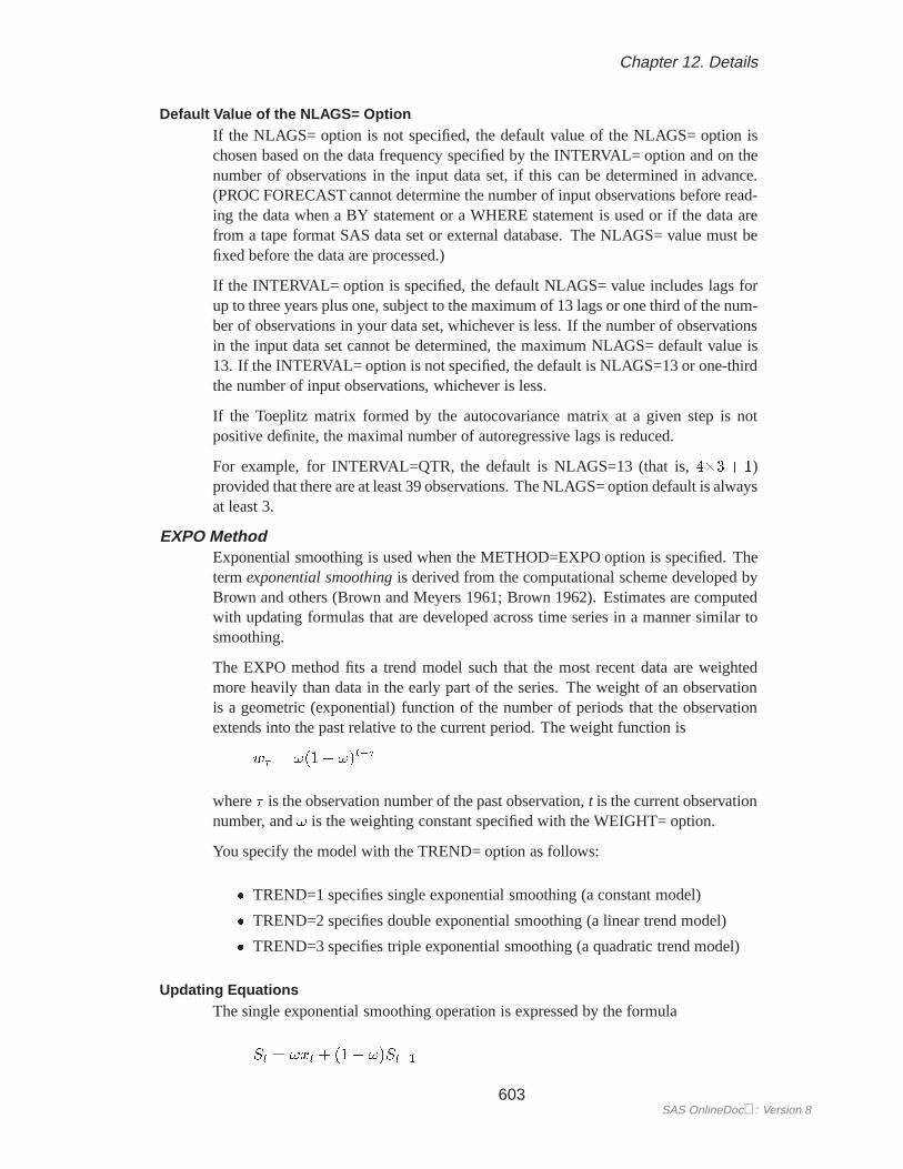
Default Value of the NLAGS= OptionIf the NLAGS= option is not specified, the default value of the NLAGS= option ischosen based on the data frequency specified by the INTERVAL= option and on thenumber of observations in the input data set, if this can be determined in advance.(PROC FORECAST cannot determine the number of input observations before read-ing the data when a BY statement or a WHERE statement is used or if the data arefrom a tape format SAS data set or external database. The NLAGS= value must befixed before the data are processed.)
If the INTERVAL= option is specified, the default NLAGS= value includes lags forup to three years plus one, subject to the maximum of 13 lags or one third of the num-ber of observations in your data set, whichever is less. If the number of observationsin the input data set cannot be determined, the maximum NLAGS= default value is13. If the INTERVAL= option is not specified, the default is NLAGS=13 or one-thirdthe number of input observations, whichever is less.
If the Toeplitz matrix formed by the autocovariance matrix at a given step is notpositive definite, the maximal number of autoregressive lags is reduced.
For example, for INTERVAL=QTR, the default is NLAGS=13 (that is,4�3 + 1)provided that there are at least 39 observations. The NLAGS= option default is alwaysat least 3.
EXPO MethodExponential smoothing is used when the METHOD=EXPO option is specified. Thetermexponential smoothingis derived from the computational scheme developed byBrown and others (Brown and Meyers 1961; Brown 1962). Estimates are computedwith updating formulas that are developed across time series in a manner similar tosmoothing.
The EXPO method fits a trend model such that the most recent data are weightedmore heavily than data in the early part of the series. The weight of an observationis a geometric (exponential) function of the number of periods that the observationextends into the past relative to the current period. The weight function is
w� = !(1� !)t��
where� is the observation number of the past observation,t is the current observationnumber, and! is the weighting constant specified with the WEIGHT= option.
You specify the model with the TREND= option as follows:
� TREND=1 specifies single exponential smoothing (a constant model)
� TREND=2 specifies double exponential smoothing (a linear trend model)
� TREND=3 specifies triple exponential smoothing (a quadratic trend model)
Updating EquationsThe single exponential smoothing operation is expressed by the formula
St = !xt + (1� !)St�1
603SAS OnlineDoc: Version 8
Part 2. General Information
whereSt is the smoothed value at the current period,t is the time index of the currentperiod, andxt is the current actual value of the series. The smoothed valueSt is theforecast ofxt+1 and is calculated as the smoothing constant! times the value of theseries,xt, in the current period plus (1� !) times the previous smoothed valueSt�1,which is the forecast ofxt computed at timet� 1.
Double and triple exponential smoothing are derived by applying exponentialsmoothing to the smoothed series, obtaining smoothed values as follows:
S[2]t = !St + (1� !)S
[2]t�1
S[3]t = !S
[2]t + (1� !)S
[3]t�1
Missing values after the start of the series are replaced with one-step-ahead predictedvalues, and the predicted value is then applied to the smoothing equations.
The polynomial time trend parameters CONSTANT, LINEAR, and QUAD in the
OUTEST= data set are computed fromST , S[2]T , andS[3]
T , the final smoothed valuesat observationT, the last observation used to fit the model. In the OUTEST= dataset, the values ofST , S[2]
T , andS[3]T are identified by–TYPE–=S1,–TYPE–=S2, and
–TYPE–=S3, respectively.
Smoothing WeightsExponential smoothing forecastsare forecasts for an integrated moving-average pro-cess; however, the weighting parameter is specified by the user rather than estimatedfrom the data. Experience has shown that good values for the WEIGHT= optionare between 0.05 and 0.3. As a general rule, smaller smoothing weights are appro-priate for series with a slowly changing trend, while larger weights are appropriatefor volatile series with a rapidly changing trend. If unspecified, the weight defaultsto (1� :81=trend), wheretrend is the value of the TREND= option. This producesdefaults of WEIGHT=0.2 for TREND=1, WEIGHT=0.10557 for TREND=2, andWEIGHT=0.07168 for TREND=3.
Confidence LimitsThe confidence limits for exponential smoothing forecasts are calculated as theywould be for an exponentially weighted time-trend regression, using the simplifyingassumption of an infinite number of observations. The variance estimate is computedusing the mean square of the unweighted one-step-ahead forecast residuals.
More detailed descriptions of the forecast computations can be found in Montgomeryand Johnson (1976) and Brown (1962).
Exponential Smoothing as an ARIMA ModelThe traditional description of exponential smoothing given in the preceding sectionis standard in most books on forecasting, and so this traditional version is employedby PROC FORECAST.
However, the standard exponential smoothing model is, in fact, a special caseof an ARIMA model (McKenzie 1984). Single exponential smoothing corre-sponds to an ARIMA(0,1,1) model; double exponential smoothing corresponds
SAS OnlineDoc: Version 8604
Chapter 12. Details
to an ARIMA(0,2,2) model; and triple exponential smoothing corresponds to anARIMA(0,3,3) model.
The traditional exponential smoothing calculations can be viewed as a simple andcomputationally inexpensive method of forecasting the equivalent ARIMA model.The exponential smoothing technique was developed in the 1960s before computerswere widely available and before ARIMA modeling methods were developed.
If you use exponential smoothing as a forecasting method, you might consider usingthe ARIMA procedure to forecast the equivalent ARIMA model as an alternative tothe traditional version of exponential smoothing used by PROC FORECAST. Theadvantages of the ARIMA form are:
� The optimal smoothing weight is automatically computed as the estimate ofthe moving average parameter of the ARIMA model.
� For double exponential smoothing, the optimal pair of two smoothing weightsare computed. For triple exponential smoothing, the optimal three smoothingweights are computed by the ARIMA method. Most implementations of thetraditional exponential smoothing method (including PROC FORECAST) usethe same smoothing weight for each stage of smoothing.
� The problem of setting the starting smoothed value is automatically handledby the ARIMA method. This is done in a statistically optimal way when themaximum likelihood method is used.
� The statistical estimates of the forecast confidence limits have a sounder theo-retical basis.
See Chapter 7, “The ARIMA Procedure,” for information on forecasting withARIMA models.
The Time Series Forecasting System provides for exponential smoothing models andallows you to either specify or optimize the smoothing weights. See Chapter 23, “Get-ting Started with Time Series Forecasting,” for details.
WINTERS MethodThe WINTERS method uses updating equations similar to exponential smoothing tofit parameters for the model
xt = (a+ bt)s(t) + �t
wherea and b are the trend parameters, and the functions(t) selects the seasonalparameter for the season corresponding to timet.
The WINTERS method assumes that the series values are positive. If negative orzero values are found in the series, a warning is printed and the values are treated asmissing.
The preceding standard WINTERS model uses a linear trend. However, PROCFORECAST can also fit a version of the WINTERS method that uses a quadratictrend. When TREND=3 is specified for METHOD=WINTERS, PROC FORECAST
605SAS OnlineDoc: Version 8
Part 2. General Information
fits the following model:
xt = (a+ bt+ ct2)s(t) + �t
The quadratic trend version of the Winters method is often unstable, and its use is notrecommended.
When TREND=1 is specified, the following constant trend version is fit:
xt = as(t) + �t
The default for the WINTERS method is TREND=2, which produces the standardlinear trend model.
Seasonal FactorsThe notations(t) represents the selection of the seasonal factor used for different timeperiods. For example, if INTERVAL=DAY and SEASONS=MONTH, there are 12seasonal factors, one for each month in the year, and the time indext is measuredin days. For any observation,t is determined by the ID variable ands(t) selects theseasonal factor for the month thatt falls in. For example, ift is 9 February 1993 thens(t) is the seasonal parameter for February.
When there are multiple seasons specified,s(t) is the product of the parameters forthe seasons. For example, if SEASONS=(MONTH DAY), thens(t) is the product ofthe seasonal parameter for the month corresponding to the periodt, and the seasonalparameter for the day of the week corresponding to periodt. When the SEASONS=option is not specified, the seasonal factorss(t) are not included in the model. Seethe section "Specifying Seasonality" later in this chapter for more information onspecifying multiple seasonal factors.
Updating EquationsThis section shows the updating equations for the Winters method. In the followingformula,xt is the actual value of the series at timet; at is the smoothed value of theseries at timet; bt is the smoothed trend at timet; ct is the smoothed quadratic trendat timet; st�1(t) selects the old value of the seasonal factor corresponding to timetbefore the seasonal factors are updated.
The estimates of the constant, linear, and quadratic trend parameters are updatedusing the following equations:
For TREND=3,
at = !1xt
st�1(t)+ (1� !1)(at�1 + bt�1 + ct�1)
bt = !2(at � at�1 + ct�1) + (1� !2)(bt�1 + 2ct�1)
ct = !21
2(bt � bt�1) + (1� !2)ct�1
SAS OnlineDoc: Version 8606
Chapter 12. Details
For TREND=2,
at = !1xt
st�1(t)+ (1� !1)(at�1 + bt�1)
bt = !2(at � at�1) + (1� !2)bt�1
For TREND=1,
at = !1xt
st�1(t)+ (1� !1)at�1
In this updating system, the trend polynomial is always centered at the current periodso that the intercept parameter of the trend polynomial for predicted values at timesaftert is always the updated intercept parameterat. The predicted value for� periodsahead is
xt+� = (at + bt�)st(t+ �)
The seasonal parameters are updated when the season changes in the data, using themean of the ratios of the actual to the predicted values for the season. For example, ifSEASONS=MONTH and INTERVAL=DAY, then, when the observation for the firstof February is encountered, the seasonal parameter for January is updated using theformula
st(t� 1) = !31
31
t�1X
i=t�31
xiai
+ (1� !3)st�1(t� 1)
wheret is February 1 of the current year andst(t� 1) is the seasonal parameter forJanuary updated with the data available at timet.
When multiple seasons are used,st(t) is a product of seasonal factors. For example,if SEASONS=(MONTH DAY) thenst(t) is the product of the seasonal factors forthe month and for the day of the week:st(t) = smt (t)s
dt (t).
The factorsmt (t) is updated at the start of each month using the preceding formula,and the factorsdt (t) is updated at the start of each week using the following formula:
sdt (t� 1) = !31
7
t�1X
i=t�7
xiai
+ (1� !3)sdt�1(t� 1)
Missing values after the start of the series are replaced with one-step-ahead predictedvalues, and the predicted value is substituted forxi and applied to the updating equa-tions.
607SAS OnlineDoc: Version 8
Part 2. General Information
NormalizationThe parameters are normalized so that the seasonal factors for each cycle have a meanof 1.0. This normalization is performed after each complete cycle and at the endof the data. Thus, if INTERVAL=MONTH and SEASONS=MONTH are specified,and a series begins with a July value, then the seasonal factors for the series arenormalized at each observation for July and at the last observation in the data set.The normalization is performed by dividing each of the seasonal parameters, andmultiplying each of the trend parameters, by the mean of the unnormalized seasonalparameters.
Smoothing WeightsThe weight for updating the seasonal factors,!3, is given by the third value specifiedin the WEIGHT= option. If the WEIGHT= option is not used, then!3 defaults to0.25; if the WEIGHT= option is used but does not specify a third value, then!3
defaults to!2. The weight for updating the linear and quadratic trend parameters,!2, is given by the second value specified in the WEIGHT= option; if the WEIGHT=option does not specify a second value, then!2 defaults to!1. The updating weightfor the constant parameter,!1, is given by the first value specified in the WEIGHT=option. As a general rule, smaller smoothing weights are appropriate for series witha slowly changing trend, while larger weights are appropriate for volatile series witha rapidly changing trend.
If the WEIGHT= option is not used, then!1 defaults to (1� :81=trend), wheretrend is the value of the TREND= option. This produces defaults of WEIGHT=0.2for TREND=1, WEIGHT=0.10557 for TREND=2, and WEIGHT=0.07168 forTREND=3.
The Time Series Forecasting System provides for generating forecast models us-ing Winters Method and allows you to specify or optimize the weights. See Chap-ter 23, “Getting Started with Time Series Forecasting,” for details.
Confidence LimitsA method for calculating exact forecast confidence limits for the WINTERS methodis not available. Therefore, the approach taken in PROC FORECAST is to assumethat the true seasonal factors have small variability about a set of fixed seasonal fac-tors and that the remaining variation of the series is small relative to the mean levelof the series. The equations are written
st(t) = I(t)(1 + �t)
xt = �I(t)(1 + t)
at = �(1 + �t)
where� is the mean level and I(t) are the fixed seasonal factors. Assuming that�tand�t are small, the forecast equations can be linearized and only first-order termsin �t and�t kept. In terms of forecasts for t, this linearized system is equivalent toa seasonal ARIMA model. Confidence limits for t are based on this ARIMA modeland converted into confidence limits forxt usingst(t) as estimates of I(t).
SAS OnlineDoc: Version 8608
Chapter 12. Details
The exponential smoothing confidence limits are based on an approximation to aweighted regression model, whereas the preceding Winters confidence limits arebased on an approximation to an ARIMA model. You can use METHOD=WINTERSwithout the SEASONS= option to do exponential smoothing and get confidence lim-its for the EXPO forecasts based on the ARIMA model approximation. These aregenerally more pessimistic than the weighted regression confidence limits producedby METHOD=EXPO.
ADDWINTERS MethodThe ADDWINTERS method is like the WINTERS method except that the seasonalparameters are added to the trend instead of multiplied with the trend. The defaultTREND=2 model is as follows:
xt = a+ bt+ s(t) + �t
The WINTERS method for updating equation and confidence limits calculations de-scribed in the preceding section are modified accordingly for the additive version.
Holt Two-Parameter Exponential SmoothingIf the seasonal factors are omitted (that is, if the SEASONS= option is not specified),the WINTERS (and ADDWINTERS) method reduces to the Holt two-parameter ver-sion of exponential smoothing. Thus, the WINTERS method is often referred to asthe Holt-Winters method.
Double exponential smoothing is a special case of the Holt two-parametersmoother. The double exponential smoothing results can be duplicated withMETHOD=WINTERS by omitting the SEASONS= option and appropriately settingthe WEIGHT= option. Letting� = !(2� !) and � = !=(2� !), the followingstatements produce the same forecasts:
proc forecast method=expo trend=2 weight= ! ... ;
proc forecast method=winters trend=2weight=( �, �) ... ;
Although the forecasts are the same, the confidence limits are computed differently.
Choice of Weights for EXPO, WINTERS, and ADDWINTERS MethodsFor the EXPO, WINTERS, and ADDWINTERS methods, properly chosen smooth-ing weights are of critical importance in generating reasonable results. There areseveral factors to consider in choosing the weights.
The noisier the data, the lower should be the weight given to the most recent ob-servation. Another factor to consider is how quickly the mean of the time series ischanging. If the mean of the series is changing rapidly, relatively more weight shouldbe given to the most recent observation. The more stable the series over time, thelower should be the weight given to the most recent observation.
Note that the smoothing weights should be set separately for each series; weightsthat produce good results for one series may be poor for another series. Since PROCFORECAST does not have a feature to use different weights for different series, whenforecasting multiple series with the EXPO, WINTERS, or ADDWINTERS method it
609SAS OnlineDoc: Version 8
Part 2. General Information
may be desirable to use different PROC FORECAST steps with different WEIGHT=options.
For the Winters method, many combinations of weight values may produce unstablenoninvertiblemodels, even though all three weights are between 0 and 1. When themodel is noninvertible, the forecasts depend strongly on values in the distant past, andpredictions are determined largely by the starting values. Unstable models usuallyproduce poor forecasts. The Winters model may be unstable even if the weightsare optimally chosen to minimize the in-sample MSE. Refer to Archibald (1990) fora detailed discussion of the unstable region of the parameter space of the Wintersmodel.
Optimal weights and forecasts for exponential smoothing models can be computedusing the ARIMA procedure. For more information, see "Exponential Smoothing asan ARIMA Model" earlier in this chapter.
The ARIMA procedure can also be used to compute optimal weights and forecastsfor seasonal ARIMA models similar to the Winters type methods. In particular, anARIMA(0,1,1)�(0,1,1)S model may be a good alternative to the additive versionof the Winters method. The ARIMA(0,1,1)�(0,1,1)S model fit to the logarithmsof the series may be a good alternative to the multiplicative Winters method. SeeChapter 7, “The ARIMA Procedure,” for information on forecasting with ARIMAmodels.
The Time Series Forecasting System can be used to automatically select an appro-priate smoothing method as well as to optimize the smoothing weights. See Chap-ter 23, “Getting Started with Time Series Forecasting,” for more information.
Starting Values for EXPO, WINTERS, and ADDWINTERS MethodsThe exponential smoothing method requires starting values for the smoothed values
S0, S[2]0 , andS [3]
0 . The Winters and additive Winters methods require starting valuesfor the trend coefficients and seasonal factors.
By default, starting values for the trend parameters are computed by a time-trendregression over the first few observations for the series. Alternatively, you can spec-ify the starting value for the trend parameters with the ASTART=, BSTART=, andCSTART= options.
The number of observations used in the time-trend regression for starting values de-pends on the NSTART= option. For METHOD=EXPO, NSTART= beginning valuesof the series are used, and the coefficients of the time-trend regression are then used
to form the initial smoothed valuesS0, S[2]0 , andS [3]
0 .
For METHOD=WINTERS or METHOD=ADDWINTERS,n complete seasonal cy-cles are used to compute starting values for the trend parameter, wheren is the valueof the NSTART= option. For example, for monthly data the seasonal cycle is oneyear, so NSTART=2 specifies that the first 24 observations at the beginning of eachseries are used for the time trend regression used to calculate starting values.
The starting values for the seasonal factors for the WINTERS and ADDWINTERSmethods are computed from seasonal averages over the first few complete seasonalcycles at the beginning of the series. The number of seasonal cycles averaged to com-
SAS OnlineDoc: Version 8610

Chapter 12. Details
pute starting seasonal factors is controlled by the NSSTART= option. For example,for monthly data with SEASONS=12 or SEASONS=MONTH, the firstn January val-ues are averaged to get the starting value for the January seasonal parameter, wherenis the value of the NSSTART= option.
Thes0(i) seasonal parameters are set to the ratio (for WINTERS) or difference (forADDWINTERS) of the mean for the season to the overall mean for the observationsused to compute seasonal starting values.
For example, if METHOD=WINTERS, INTERVAL=DAY, SEASON=(MONTHDAY), and NSTART=2 (the default), the initial seasonal parameter for January isthe ratio of the mean value over days in the first two Januarys after the start of theseries (that is, after the first nonmissing value), to the mean value for all days readfor initialization of the seasonal factors. Likewise, the initial factor for Sundays is theratio of the mean value for Sundays to the mean of all days read.
For the ASTART=, BSTART=, and CSTART= options, the values specified are asso-ciated with the variables in the VAR statement in the order in which the variables arelisted (the first value with the first variable, the second value with the second variable,and so on). If there are fewer values than variables, default starting values are usedfor the later variables. If there are more values than variables, the extra values areignored.
Specifying Seasonality
Seasonalityof a time series is a regular fluctuation about a trend. This is calledseasonality because the time of year is the most common source of periodic variation.For example, sales of home heating oil are regularly greater in winter than duringother times of the year.
Seasonality can be caused by many things other than weather. In the United States,sales of nondurable goods are greater in December than in other months becauseof the Christmas shopping season. The term seasonality is also used for cyclicalfluctuation at periods other than a year. Often, certain days of the week cause regularfluctuation in daily time series, such as increased spending on leisure activities duringweekends.
Three kinds of seasonality are supported in PROC FORECAST: time-of-year, day-of-week, and time-of-day. The seasonal part of the model is specified using the SEA-SONS= option. The values for the SEASONS= option are listed in Table 12.1.
Table 12.1. The SEASONS= Option
SEASONS= Value Cycle Length Type of SeasonalityQTR yearly time of yearMONTH yearly time of yearDAY weekly day of weekHOUR daily time of day
611SAS OnlineDoc: Version 8
Part 2. General Information
The three kinds of seasonality can be combined. For example, SEASONS=(MONTHDAY HOUR) specifies that 24 hour-of-day seasons are nested within 7 day-of-weekseasons, which in turn are nested within 12 month-of-year seasons. The differentkinds of intervals can be listed in the SEASONS= option in any order. Thus, SEA-SONS=(HOUR DAY MONTH) is the same as SEASONS=(MONTH DAY HOUR).Note that the Winters method smoothing equations may be less stable when multipleseasonal factors are used.
Multiple period seasons can also be used. For example, SEASONS=QTR2 specifiestwo semiannual time-of-year seasons. The grouping of observations into multiple pe-riod seasons starts with the first interval in the seasonal cycle. Thus, MONTH2 sea-sons are January-February, March-April, and so on. (There is no provision for shift-ing seasonal intervals; thus, there is no way to specify December-January, February-March, April-May, and so on seasons.)
For multiple period seasons, the number of intervals combined to form the seasonsmust evenly divide and be less than the basic cycle length. For example, with SEA-SONS=MONTHn, the basic cycle length is 12, so MONTH2, MONTH3, MONTH4,and MONTH6 are valid SEASONS= values (since 2, 3, 4, and 6 evenly divide 12 andare less than 12), but MONTH5 and MONTH12 are not valid SEASONS= values.
The frequency of the seasons must not be greater than the frequency of the inputdata. For example, you cannot specify SEASONS=MONTH if INTERVAL=QTR orSEASONS=MONTH if INTERVAL=MONTH2. You also cannot specify two sea-sons of the same basic cycle. For example, SEASONS=(MONTH QTR) or SEA-SONS=(MONTH2 MONTH4) is not allowed.
Alternatively, the seasonality can be specified by giving the number of seasons in theSEASONS= option. SEASONS=n specifies that there aren seasons, with observa-tions 1,n+1, 2n+1, and so on in the first season, observations 2,n+2, 2n+2, and so onin the second season, and so forth.
The options SEASONS=n and SINTPER=m cause PROC FORECAST to group theinput observations intonseasons, withmobservations to a season, which repeat everynm observations. The options SEASONS=(n1 n2) and SINTPER=(m1 m2) producen1 seasons withm1 observations to a season nested withinn2 seasons withn1m1m2
observations to a season.
If the SINTPER=m option is used with the SEASONS= option, the SEASONS=interval is multiplied by the SINTPER= value. For example, specifying bothSEASONS=(QTR HOUR) and SINTPER=(2 3) is the same as specifying SEA-SONS=(QTR2 HOUR3) and also the same as specifying SEASONS=(HOUR3QTR2).
SAS OnlineDoc: Version 8612
Chapter 12. Details
Data Requirements
You should have ample data for the series that you forecast using PROC FORECAST.However, the results may be poor unless you have a good deal more than the min-imum amount of data the procedure allows. The minimum number of observationsrequired for the different methods is as follows:
� If METHOD=STEPAR is used, the minimum number of nonmissing observa-tions required for each series forecast is the TREND= option value plus thevalue of the NLAGS= option. For example, using NLAGS=13 and TREND=2,at least 15 nonmissing observations are needed.
� If METHOD=EXPO is used, the minimum is the TREND= option value.
� If METHOD=WINTERS or ADDWINTERS is used, the minimum number ofobservations is either the number of observations in a complete seasonal cycleor the TREND= option value, whichever is greater. (However, there should bedata for several complete seasonal cycles, or the seasonal factor estimates maybe poor.) For example, for the seasonal specifications SEASONS=MONTH,SEASONS=(QTR DAY), or SEASONS=(MONTH DAY HOUR), the longestcycle length is one year, so at least one year of data is required.
OUT= Data Set
The FORECAST procedure writes the forecast to the output data set named by theOUT= option. The OUT= data set contains the following variables:
� the BY variables
� –TYPE–, a character variable that identifies the type of observation
� –LEAD–, a numeric variable that indicates the number of steps ahead in theforecast. The value of–LEAD– is 0 for the one-step-ahead forecasts beforethe start of the forecast period.
� the ID statement variables
� the VAR statement variables, which contain the result values as indicated bythe–TYPE– variable value for the observation
The FORECAST procedure processes each of the input variables listed in the VARstatement and writes several observations for each forecast period to the OUT= dataset. The observations are identified by the value of the–TYPE– variable. The optionsOUTACTUAL, OUTALL, OUTLIMIT, OUTRESID, OUT1STEP, OUTFULL, andOUTSTD control which types of observations are included in the OUT= data set.
The values of the variable–TYPE– are as follows:
ACTUAL The VAR statement variables contain actual values from the inputdata set. The OUTACTUAL option writes the actual values. Bydefault, only the observations for the forecast period are output.
613SAS OnlineDoc: Version 8

Part 2. General Information
FORECAST The VAR statement variables contain forecast values. TheOUT1STEP option writes the one-step-ahead predicted valuesfor the observations used to fit the model.
RESIDUAL The VAR statement variables contain residuals. The residuals arecomputed by subtracting the forecast value from the actual value(residual = actual � forecast). The OUTRESID option writesobservations for the residuals.
Lnn The VAR statement variables contain lowernn% confidence limitsfor the forecast values. The value ofnn depends on the ALPHA=option; with the default ALPHA=0.05, the–TYPE– value is L95for the lower confidence limit observations. The OUTLIMIT op-tion writes observations for the upper and lower confidence limits.
Unn The VAR statement variables contain uppernn% confidence limitsfor the forecast values. The value ofnn depends on the ALPHA=option; with the default ALPHA=0.05, the–TYPE– value is U95for the upper confidence limit observations. The OUTLIMIT op-tion writes observations for the upper and lower confidence limits.
STD The VAR statement variables contain standard errors of the forecastvalues. The OUTSTD option writes observations for the standarderrors of the forecast.
If no output control options are specified, PROC FORECAST outputs only the fore-cast values for the forecast periods.
The –TYPE– variable can be used to subset the OUT= data set. For example, thefollowing data step splits the OUT= data set into two data sets, one containing theforecast series and the other containing the residual series. For example
proc forecast out=out outresid ...;...
run;
data fore resid;set out;if _TYPE_=’FORECAST’ then output fore;if _TYPE_=’RESIDUAL’ then output resid;
run;
See Chapter 2, “Working with Time Series Data,” for more information on processingtime series data sets in this format.
SAS OnlineDoc: Version 8614
Chapter 12. Details
OUTEST= Data Set
The FORECAST procedure writes the parameter estimates and goodness-of-fit statis-tics to an output data set when the OUTEST= option is specified. The OUTEST= dataset contains the following variables:
� the BY variables
� the first ID variable, which contains the value of the ID variable for the lastobservation in the input data set used to fit the model
� –TYPE–, a character variable that identifies the type of each observation
� the VAR statement variables, which contain statistics and parameter estimatesfor the input series. The values contained in the VAR statement variables de-pend on the–TYPE– variable value for the observation.
The observations contained in the OUTEST= data set are identified by the–TYPE–variable. The OUTEST= data set may contain observations with the following
–TYPE– values:
AR1–ARn The observation contains estimates of the autoregressive parame-ters for the series. Two-digit lag numbers are used if the value ofthe NLAGS= option is 10 or more; in that case these–TYPE–values are AR01–ARn. These observations are output for theSTEPAR method only.
CONSTANT The observation contains the estimate of the constant or interceptparameter for the time-trend model for the series. For the expo-nential smoothing and the Winters’ methods, the trend model iscentered (that is,t=0) at the last observation used for the fit.
LINEAR The observation contains the estimate of the linear or slope param-eter for the time-trend model for the series. This observation isoutput only if you specify TREND=2 or TREND=3.
N The observation contains the number of nonmissing observationsused to fit the model for the series.
QUAD The observation contains the estimate of the quadratic parameterfor the time-trend model for the series. This observation is outputonly if you specify TREND=3.
SIGMA The observation contains the estimate of the standard deviation ofthe error term for the series.
S1–S3 The observations contain exponentially smoothed values at the lastobservation.–TYPE–=S1 is the final smoothed value of the singleexponential smooth.–TYPE–=S2 is the final smoothed value ofthe double exponential smooth.–TYPE–=S3 is the final smoothedvalue of the triple exponential smooth. These observations are out-put for METHOD=EXPO only.
615SAS OnlineDoc: Version 8
Part 2. General Information
S–name The observation contains estimates of the seasonal parameters.For example, if SEASONS=MONTH, the OUTEST= data set willcontain observations with–TYPE–=S–JAN, –TYPE–=S–FEB,
–TYPE–=S–MAR, and so forth.
For multiple-period seasons, the names of the first and last intervalof the season are concatenated to form the season name. Thus, forSEASONS=MONTH4, the OUTEST= data set will contain obser-vations with–TYPE–=S–JANAPR,–TYPE–=S–MAYAUG, and
–TYPE–=S–SEPDEC.
When the SEASONS= option specifies numbers, the seasonal fac-tors are labeled–TYPE–=S–i–j. For example, SEASONS=(2 3)produces observations with–TYPE– values of S–1–1, S–1–2,S–2–1, S–2–2, and S–2–3. The observation with–TYPE–=S–i–jcontains the seasonal parameters for thejth season of theith sea-sonal cycle.
These observations are output only for METHOD=WINTERS orMETHOD=ADDWINTERS.
WEIGHT The observation contains the smoothing weight used for exponen-tial smoothing. This is the value of the WEIGHT= option. Thisobservation is output for METHOD=EXPO only.
WEIGHT1
WEIGHT2
WEIGHT3 The observations contain the weights used for smoothing theWINTERS or ADDWINTERS method parameters (specified bythe WEIGHT= option). –TYPE–=WEIGHT1 is the weight usedto smooth the CONSTANT parameter.–TYPE–=WEIGHT2 isthe weight used to smooth the LINEAR and QUAD parameters.
–TYPE–=WEIGHT3 is the weight used to smooth the seasonalparameters. These observations are output only for the WINTERSand ADDWINTERS methods.
NRESID The observation contains the number of nonmissing residuals,n,used to compute the goodness-of-fit statistics. The residuals areobtained by subtracting the one-step-ahead predicted values fromthe observed values.
SST The observation contains the total sum of squares for the series,corrected for the mean.SST =
Pnt=0 (yt � y)2, wherey is the
series mean.
SSE The observation contains the sum of the squared residuals, uncor-rected for the mean.SSE =
Pnt=0 (yt � yt)
2, wherey is the one-step predicted value for the series.
MSE The observation contains the mean squared error, calculated fromone-step-ahead forecasts.MSE = 1
n�kSSE, wherek is the num-ber of parameters in the model.
SAS OnlineDoc: Version 8616
Chapter 12. Details
RMSE The observation contains the root mean square error.
RMSE =pMSE.
MAPE The observation contains the mean absolute percent error.
MAPE = 100n
Pnt=0 j(yt � yt)=ytj.
MPE The observation contains the mean percent error.
MPE = 100n
Pnt=0 (yt � yt)=yt.
MAE The observation contains the mean absolute error.
MAE = 1n
Pnt=0 jyt � ytj.
ME The observation contains the mean error.
MAE = 1n
Pnt=0 (yt � yt).
MAXE The observation contains the maximum error (the largest residual).
MINE The observation contains the minimum error (the smallest resid-ual).
MAXPE The observation contains the maximum percent error.
MINPE The observation contains the minimum percent error.
RSQUARE The observation contains the R2 statistic,R2 = 1� SSE=SST . Ifthe model fits the series badly, the model error sum of squaresSSEmay be larger thanSSTand the R2 statistic will be negative.
ADJRSQ The observation contains the adjusted R2 statistic.
ADJRSQ = 1� (n�1n�k )(1�R2).
ARSQ The observation contains Amemiya’s adjusted R2 statistic.
ARSQ = 1� (n+kn�k )(1�R2).
RW–RSQ The observation contains the random walk R2 statistic (Har-vey’sR2
D statistic using the random walk model for comparison).RW–RSQ = 1� (n�1n )SSE=RWSSE, where
RWSSE =Pn
t=2 (yt � yt�1 � �)2,
and
� = 1n�1
Pnt=2 (yt � yt�1).
AIC The observation contains Akaike’s information criterion.
AIC = nln(SSE=n) + 2k.
SBC The observation contains Schwarz’s Bayesian criterion.
SBC = nln(SSE=n) + kln(n).
APC The observation contains Amemiya’s prediction criterion.
APC = 1nSST (
n+kn�k )(1�R2) = (n+k
n�k )1nSSE.
CORR The observation contains the correlation coefficient between theactual values and the one-step-ahead predicted values.
617SAS OnlineDoc: Version 8

Part 2. General Information
THEILU The observation contains Theil’s U statistic using original units.Refer to Maddala (1977, pp. 344-345), and Pindyck and Rubinfeld(1981, pp. 364-365) for more information on Theil statistics.
RTHEILU The observation contains Theil’s U statistic calculated using rela-tive changes.
THEILUM The observation contains the bias proportion of Theil’s U statistic.
THEILUS The observation contains the variance proportion of Theil’s Ustatistic.
THEILUC The observation contains the covariance proportion of Theil’s Ustatistic.
THEILUR The observation contains the regression proportion of Theil’s Ustatistic.
THEILUD The observation contains the disturbance proportion of Theil’s Ustatistic.
RTHEILUM The observation contains the bias proportion of Theil’s U statistic,calculated using relative changes.
RTHEILUS The observation contains the variance proportion of Theil’s Ustatistic, calculated using relative changes.
RTHEILUC The observation contains the covariance proportion of Theil’s Ustatistic, calculated using relative changes.
RTHEILUR The observation contains the regression proportion of Theil’s Ustatistic, calculated using relative changes.
RTHEILUD The observation contains the disturbance proportion of Theil’s Ustatistic, calculated using relative changes.
SAS OnlineDoc: Version 8618

Chapter 12. Examples
Examples
Example 12.1. Forecasting Auto Sales
This example uses the Winters method to forecast the monthly U.S. sales of passengercars series (VEHICLES) from the data set SASHELP.USECON. These data are takenfrom Business Statistics, published by the U.S. Bureau of Economic Analysis.
The following statements plot the series; the plot is shown in Output 12.1.1:
title1 "Sales of Passenger Cars";
symbol1 i=spline v=dot;axis2 label=(a=-90 r=90 "Vehicles and Parts" )
order=(6000 to 24000 by 3000) ;proc gplot data=sashelp.usecon;
plot vehicles * date = 1 /haxis= ’1jan80’d to ’1jan92’d by yearvaxis=axis2;
where date >= ’1jan80’d;format date year4.;
run;
Output 12.1.1. Monthly Passenger Car Sales
619SAS OnlineDoc: Version 8
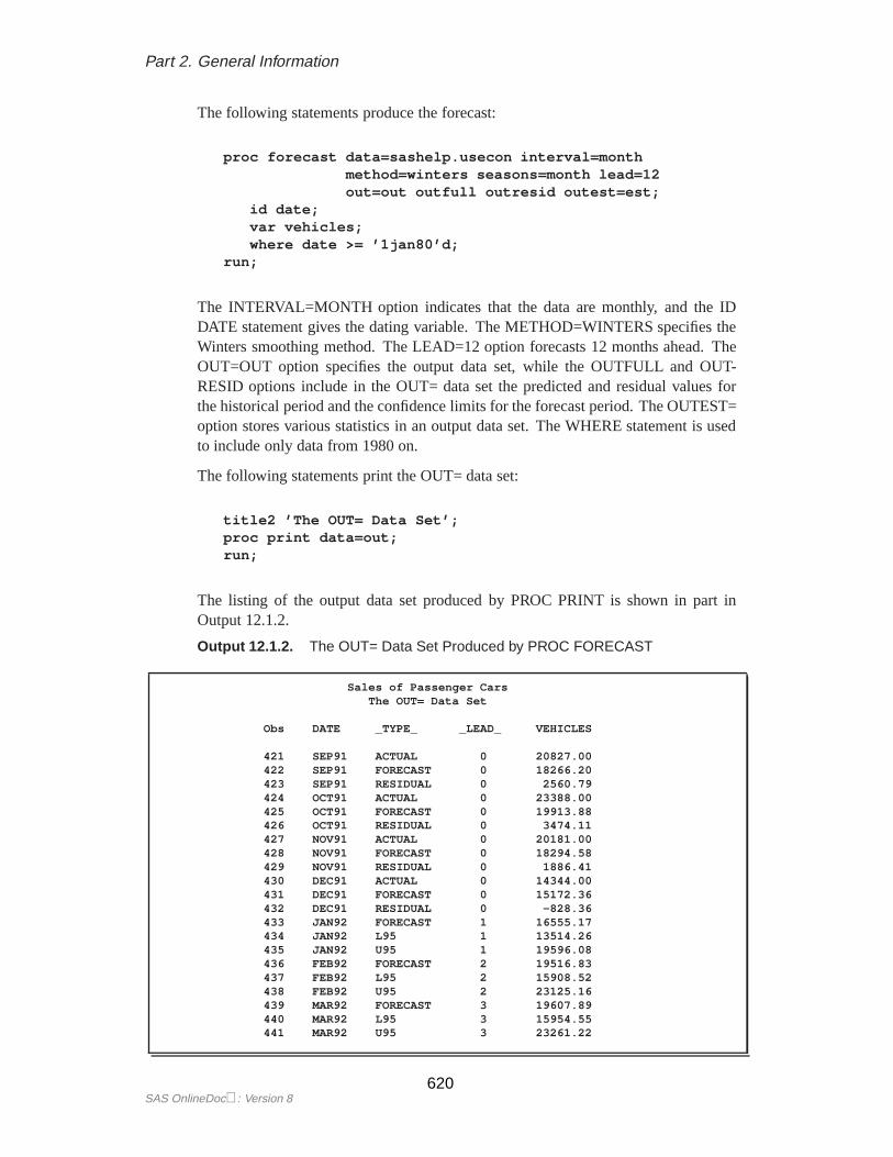
Part 2. General Information
The following statements produce the forecast:
proc forecast data=sashelp.usecon interval=monthmethod=winters seasons=month lead=12out=out outfull outresid outest=est;
id date;var vehicles;where date >= ’1jan80’d;
run;
The INTERVAL=MONTH option indicates that the data are monthly, and the IDDATE statement gives the dating variable. The METHOD=WINTERS specifies theWinters smoothing method. The LEAD=12 option forecasts 12 months ahead. TheOUT=OUT option specifies the output data set, while the OUTFULL and OUT-RESID options include in the OUT= data set the predicted and residual values forthe historical period and the confidence limits for the forecast period. The OUTEST=option stores various statistics in an output data set. The WHERE statement is usedto include only data from 1980 on.
The following statements print the OUT= data set:
title2 ’The OUT= Data Set’;proc print data=out;run;
The listing of the output data set produced by PROC PRINT is shown in part inOutput 12.1.2.
Output 12.1.2. The OUT= Data Set Produced by PROC FORECAST
Sales of Passenger CarsThe OUT= Data Set
Obs DATE _TYPE_ _LEAD_ VEHICLES
421 SEP91 ACTUAL 0 20827.00422 SEP91 FORECAST 0 18266.20423 SEP91 RESIDUAL 0 2560.79424 OCT91 ACTUAL 0 23388.00425 OCT91 FORECAST 0 19913.88426 OCT91 RESIDUAL 0 3474.11427 NOV91 ACTUAL 0 20181.00428 NOV91 FORECAST 0 18294.58429 NOV91 RESIDUAL 0 1886.41430 DEC91 ACTUAL 0 14344.00431 DEC91 FORECAST 0 15172.36432 DEC91 RESIDUAL 0 -828.36433 JAN92 FORECAST 1 16555.17434 JAN92 L95 1 13514.26435 JAN92 U95 1 19596.08436 FEB92 FORECAST 2 19516.83437 FEB92 L95 2 15908.52438 FEB92 U95 2 23125.16439 MAR92 FORECAST 3 19607.89440 MAR92 L95 3 15954.55441 MAR92 U95 3 23261.22
SAS OnlineDoc: Version 8620

Chapter 12. Examples
The following statements print the OUTEST= data set:
title2 ’The OUTEST= Data Set: WINTERS Method’;proc print data=est;run;
The PROC PRINT listing of the OUTEST= data set is shown in Output 12.1.3.
Output 12.1.3. The OUTEST= Data Set Produced by PROC FORECAST
Sales of Passenger CarsThe OUTEST= Data Set: WINTERS Method
Obs _TYPE_ DATE VEHICLES
1 N DEC91 1442 NRESID DEC91 1443 DF DEC91 1304 WEIGHT1 DEC91 0.10557285 WEIGHT2 DEC91 0.10557286 WEIGHT3 DEC91 0.257 SIGMA DEC91 1741.4818 CONSTANT DEC91 18577.3689 LINEAR DEC91 4.804732
10 S_JAN DEC91 0.890917311 S_FEB DEC91 1.050027812 S_MAR DEC91 1.054653913 S_APR DEC91 1.07495514 S_MAY DEC91 1.116612115 S_JUN DEC91 1.101297216 S_JUL DEC91 0.741829717 S_AUG DEC91 0.963388818 S_SEP DEC91 1.05115919 S_OCT DEC91 1.139912620 S_NOV DEC91 1.013212621 S_DEC DEC91 0.80203422 SST DEC91 2.63312E923 SSE DEC91 39425827024 MSE DEC91 3032755.925 RMSE DEC91 1741.48126 MAPE DEC91 9.480021727 MPE DEC91 -1.04995628 MAE DEC91 1306.853429 ME DEC91 -42.9537630 RSQUARE DEC91 0.8502696
The following statements plot the residuals. The plot is shown in Output 12.1.4.
title2 ’Plot of Residuals’;symbol1 i=needle;axis2 label=( a=-90 r=90 "Vehicles and Parts" );proc gplot data=out;
plot vehicles * date = 1 / vref=0haxis= ’1jan80’d to ’1jan92’d by yearvaxis=axis2;
where _type_ = ’RESIDUAL’;format date year4.;
run;
621SAS OnlineDoc: Version 8
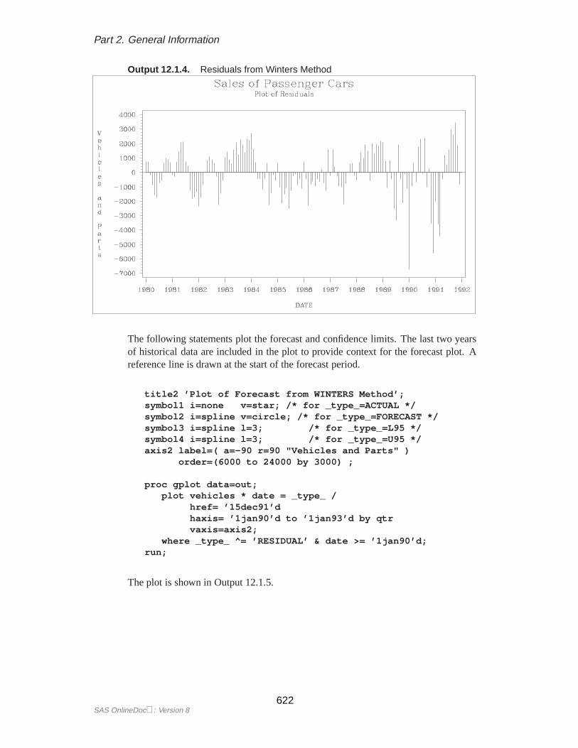
Part 2. General Information
Output 12.1.4. Residuals from Winters Method
The following statements plot the forecast and confidence limits. The last two yearsof historical data are included in the plot to provide context for the forecast plot. Areference line is drawn at the start of the forecast period.
title2 ’Plot of Forecast from WINTERS Method’;symbol1 i=none v=star; /* for _type_=ACTUAL */symbol2 i=spline v=circle; /* for _type_=FORECAST */symbol3 i=spline l=3; /* for _type_=L95 */symbol4 i=spline l=3; /* for _type_=U95 */axis2 label=( a=-90 r=90 "Vehicles and Parts" )
order=(6000 to 24000 by 3000) ;
proc gplot data=out;plot vehicles * date = _type_ /
href= ’15dec91’dhaxis= ’1jan90’d to ’1jan93’d by qtrvaxis=axis2;
where _type_ ^= ’RESIDUAL’ & date >= ’1jan90’d;run;
The plot is shown in Output 12.1.5.
SAS OnlineDoc: Version 8622

Chapter 12. Examples
Output 12.1.5. Forecast of Passenger Car Sales
Example 12.2. Forecasting Retail Sales
This example uses the stepwise autoregressive method to forecast the monthly U.S.sales of durable goods (DURABLES) and nondurable goods (NONDUR) from theSASHELP.USECON data set. The data are fromBusiness Statisticspublished by theU.S. Bureau of Economic Analysis. The following statements plot the series:
symbol1 i=spline v=dot;proc gplot data=sashelp.usecon;
plot ( durables nondur ) * date = 1 /haxis= ’1jan80’d to ’1jan92’d by year;
where date >= ’1jan80’d;format date year4.;
run;
The plots are shown in Output 12.2.1 and Output 12.2.2.
623SAS OnlineDoc: Version 8
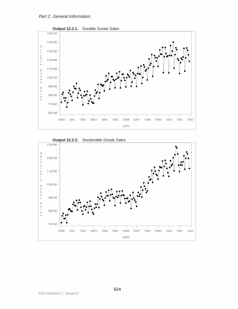
Part 2. General Information
Output 12.2.1. Durable Goods Sales
Output 12.2.2. Nondurable Goods Sales
SAS OnlineDoc: Version 8624
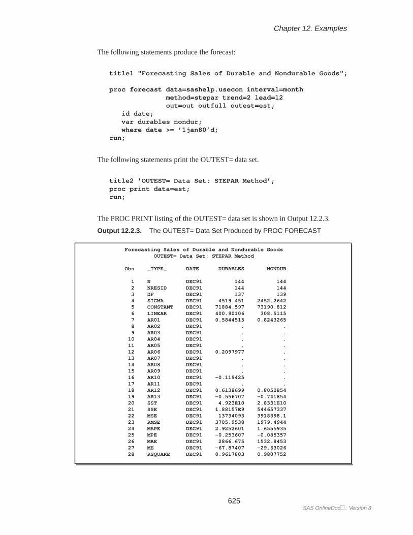
Chapter 12. Examples
The following statements produce the forecast:
title1 "Forecasting Sales of Durable and Nondurable Goods";
proc forecast data=sashelp.usecon interval=monthmethod=stepar trend=2 lead=12out=out outfull outest=est;
id date;var durables nondur;where date >= ’1jan80’d;
run;
The following statements print the OUTEST= data set.
title2 ’OUTEST= Data Set: STEPAR Method’;proc print data=est;run;
The PROC PRINT listing of the OUTEST= data set is shown in Output 12.2.3.
Output 12.2.3. The OUTEST= Data Set Produced by PROC FORECAST
Forecasting Sales of Durable and Nondurable GoodsOUTEST= Data Set: STEPAR Method
Obs _TYPE_ DATE DURABLES NONDUR
1 N DEC91 144 1442 NRESID DEC91 144 1443 DF DEC91 137 1394 SIGMA DEC91 4519.451 2452.26425 CONSTANT DEC91 71884.597 73190.8126 LINEAR DEC91 400.90106 308.51157 AR01 DEC91 0.5844515 0.82432658 AR02 DEC91 . .9 AR03 DEC91 . .
10 AR04 DEC91 . .11 AR05 DEC91 . .12 AR06 DEC91 0.2097977 .13 AR07 DEC91 . .14 AR08 DEC91 . .15 AR09 DEC91 . .16 AR10 DEC91 -0.119425 .17 AR11 DEC91 . .18 AR12 DEC91 0.6138699 0.805085419 AR13 DEC91 -0.556707 -0.74185420 SST DEC91 4.923E10 2.8331E1021 SSE DEC91 1.88157E9 54465733722 MSE DEC91 13734093 3918398.123 RMSE DEC91 3705.9538 1979.494424 MAPE DEC91 2.9252601 1.655593525 MPE DEC91 -0.253607 -0.08535726 MAE DEC91 2866.675 1532.845327 ME DEC91 -67.87407 -29.6302628 RSQUARE DEC91 0.9617803 0.9807752
625SAS OnlineDoc: Version 8
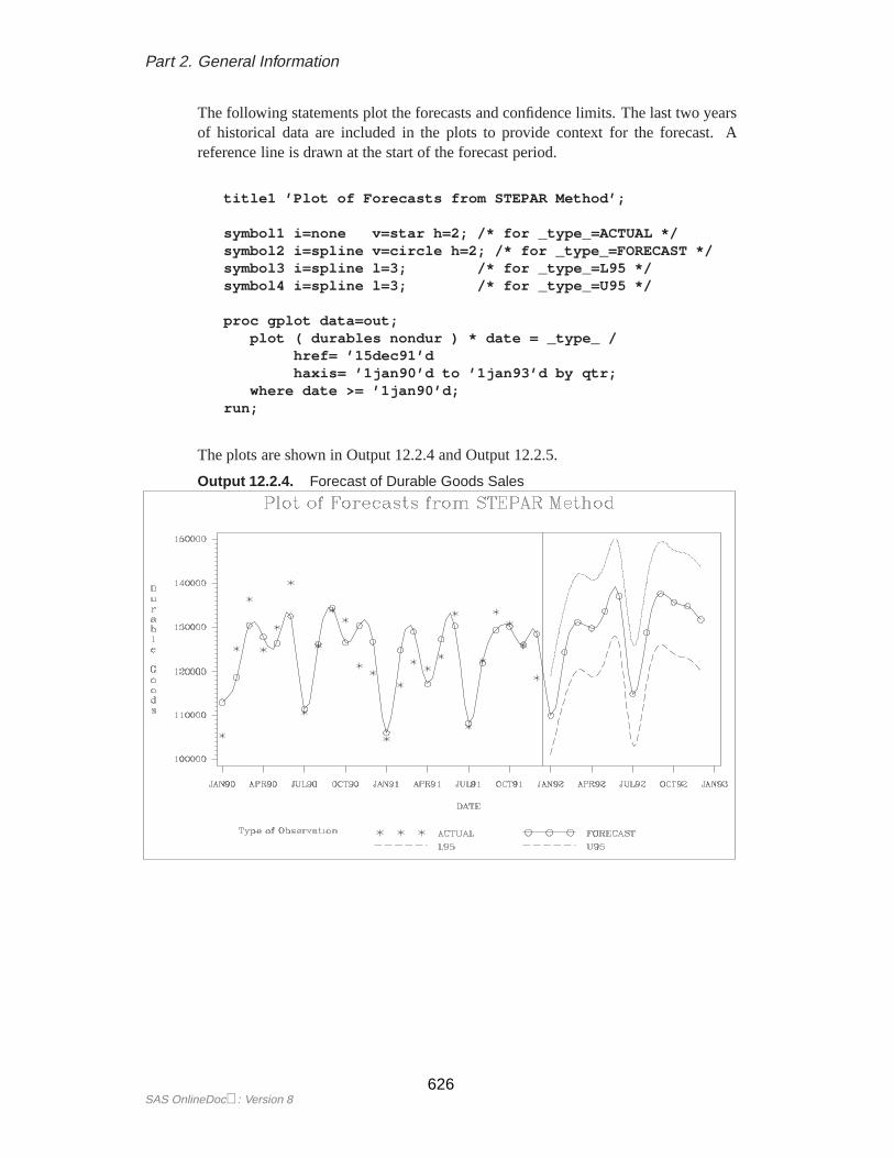
Part 2. General Information
The following statements plot the forecasts and confidence limits. The last two yearsof historical data are included in the plots to provide context for the forecast. Areference line is drawn at the start of the forecast period.
title1 ’Plot of Forecasts from STEPAR Method’;
symbol1 i=none v=star h=2; /* for _type_=ACTUAL */symbol2 i=spline v=circle h=2; /* for _type_=FORECAST */symbol3 i=spline l=3; /* for _type_=L95 */symbol4 i=spline l=3; /* for _type_=U95 */
proc gplot data=out;plot ( durables nondur ) * date = _type_ /
href= ’15dec91’dhaxis= ’1jan90’d to ’1jan93’d by qtr;
where date >= ’1jan90’d;run;
The plots are shown in Output 12.2.4 and Output 12.2.5.
Output 12.2.4. Forecast of Durable Goods Sales
SAS OnlineDoc: Version 8626
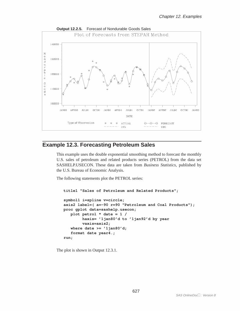
Chapter 12. Examples
Output 12.2.5. Forecast of Nondurable Goods Sales
Example 12.3. Forecasting Petroleum Sales
This example uses the double exponential smoothing method to forecast the monthlyU.S. sales of petroleum and related products series (PETROL) from the data setSASHELP.USECON. These data are taken fromBusiness Statistics, published bythe U.S. Bureau of Economic Analysis.
The following statements plot the PETROL series:
title1 "Sales of Petroleum and Related Products";
symbol1 i=spline v=circle;axis2 label=( a=-90 r=90 "Petroleum and Coal Products");proc gplot data=sashelp.usecon;
plot petrol * date = 1 /haxis= ’1jan80’d to ’1jan92’d by yearvaxis=axis2;
where date >= ’1jan80’d;format date year4.;
run;
The plot is shown in Output 12.3.1.
627SAS OnlineDoc: Version 8
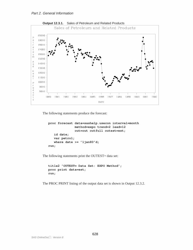
Part 2. General Information
Output 12.3.1. Sales of Petroleum and Related Products
The following statements produce the forecast:
proc forecast data=sashelp.usecon interval=monthmethod=expo trend=2 lead=12out=out outfull outest=est;
id date;var petrol;where date >= ’1jan80’d;
run;
The following statements print the OUTEST= data set:
title2 ’OUTEST= Data Set: EXPO Method’;proc print data=est;run;
The PROC PRINT listing of the output data set is shown in Output 12.3.2.
SAS OnlineDoc: Version 8628

Chapter 12. Examples
Output 12.3.2. The OUTEST= Data Set Produced by PROC FORECAST
OUTEST= Data Set: EXPO Method
Obs _TYPE_ DATE PETROL
1 N DEC91 1442 NRESID DEC91 1443 DF DEC91 1424 WEIGHT DEC91 0.10557285 S1 DEC91 14165.2596 S2 DEC91 13933.4357 SIGMA DEC91 1281.09458 CONSTANT DEC91 14397.0849 LINEAR DEC91 27.363164
10 SST DEC91 1.17001E911 SSE DEC91 23305083812 MSE DEC91 1641203.113 RMSE DEC91 1281.094514 MAPE DEC91 6.551446715 MPE DEC91 -0.14716816 MAE DEC91 891.0424317 ME DEC91 8.214858418 RSQUARE DEC91 0.8008122
The plot of the forecast is shown in Output 12.3.3.
Output 12.3.3. Forecast of Petroleum and Related Products
629SAS OnlineDoc: Version 8

Part 2. General Information
References
Ahlburg, D. A. (1984). "Forecast evaluation and improvement using Theil’s decom-position."Journal of Forecasting, 3, 345-351.
Aldrin, M. and Damsleth, E. (1989). "Forecasting non-seasonal time series withmissing observations."Journal of Forecasting, 8, 97-116.
Archibald, B.C. (1990), "Parameter space of the Holt-Winters’ model."InternationalJournal of Forecasting, 6, 199-209.
Bails, D.G. and Peppers, L.C. (1982),Business Fluctuations: Forecasting Techniquesand Applications,New Jersey: Prentice-Hall.
Bartolomei, S.M. and Sweet, A.L. (1989). "A note on the comparison of exponen-tial smoothing methods for forecasting seasonal series."International Journal ofForecasting, 5, 111-116.
Bureau of Economic Analysis, U.S. Department of Commerce (1992 and earlier edi-tions), Business Statistics, 27th and earlier editions, Washington: U.S. Govern-ment Printing Office.
Bliemel, F. (1973). "Theil’s forecast accuracy coefficient: a clarification."Journal ofMarketing Research, 10, 444-446.
Bowerman, B.L. and O’Connell, R.T. (1979),Time Series and Forecasting: An Ap-plied Approach,North Scituate, Massachusetts: Duxbury Press.
Box, G.E.P. and Jenkins, G.M. (1976),Time Series Analysis: Forecasting and Con-trol, Revised Edition, San Francisco: Holden-Day.
Bretschneider, S.I., Carbone, R., and Longini, R.L. (1979). "An adaptive approach totime series forecasting."Decision Sciences, 10, 232-244.
Brown, R.G. (1962),Smoothing, Forecasting and Prediction of Discrete Time Series,New York: Prentice-Hall.
Brown, R.G. and Meyer, R.F. (1961). "The fundamental theorem of exponentialsmoothing."Operations Research, 9, 673-685.
Chatfield, C. (1978). "The Holt-Winters forecasting procedure."Applied Statistics,27, 264-279.
Chatfield, C., and Prothero, D.L. (1973). "Box-Jenkins seasonal forecasting: prob-lems in a case study."Journal of the Royal Statistical Society, Series A, 136,295-315.
Chow, W.M. (1965). "Adaptive control of the exponential smoothing constant."Jour-nal of Industrial Engineering, September-October 1965.
Cogger, K.O. (1974). "The optimality of general-order exponential smoothing."Op-erations Research, 22, 858-.
Cox, D. R. (1961). "Prediction by exponentially weighted moving averages and re-lated methods."Journal of the Royal Statistical Society, Series B, 23, 414-422.
SAS OnlineDoc: Version 8630
Chapter 12. References
Fair, R.C. (1986). "Evaluating the predictive accuracy of models." InHandbook ofEconometrics, Vol. 3., Griliches, Z. and Intriligator, M.D., eds. New York: NorthHolland.
Fildes, R. (1979). "Quantitative forecasting — the state of the art: extrapolativemodels."Journal of Operational Research Society, 30, 691-710.
Gardner, E.S. (1984). "The strange case of the lagging forecasts."Interfaces, 14,47-50.
Gardner, E.S., Jr. (1985). "Exponential smoothing: the state of the art."Journal ofForecasting, 4, 1-38.
Granger, C.W.J. and Newbold, P. (1977),Forecasting Economic Time Series, NewYork: Academic Press, Inc.
Harvey, A.C. (1984). "A unified view of statistical forecasting procedures."Journalof Forecasting, 3, 245-275.
Ledolter, J. and Abraham, B. (1984). "Some comments on the initialization of expo-nential smoothing."Journal of Forecasting, 3, 79-84.
Maddala, G.S. (1977),Econometrics, New York: McGraw-Hill Book Co.
Makridakis, S., Wheelwright, S.C., and McGee, V.E. (1983).Forecasting: Methodsand Applications, 2nd Ed.New York: John Wiley and Sons.
McKenzie, Ed (1984). "General exponential smoothing and the equivalent ARMAprocess."Journal of Forecasting, 3, 333-344.
Montgomery, D.C. and Johnson, L.A. (1976),Forecasting and Time Series Analysis,New York: McGraw-Hill Book Co.
Muth, J.F. (1960). "Optimal properties of exponentially weighted forecasts."Journalof the American Statistical Association, 55, 299-306.
Pierce, D.A. (1979). "R2 Measures for Time Series."Journal of the American Statis-tical Association, 74, 901-910.
Pindyck, R.S. and Rubinfeld, D.L. (1981),Econometric Models and Economic Fore-casts, Second Edition, New York: McGraw-Hill Book Co.
Raine, J.E. (1971). "Self-adaptive forecasting reconsidered."Decision Sciences, 2,181-191.
Roberts, S.A. (1982). "A general class of Holt-Winters type forecasting models."Management Science, 28, 808-820.
Theil, H. (1966).Applied Economic Forecasting. Amsterdam: North Holland.
Trigg, D.W., and Leach, A.G. (1967). "Exponential smoothing with an adaptive re-sponse rate."Operational Research Quarterly, 18, 53-59.
Winters, P.R. (1960). "Forecasting sales by exponentially weighted moving aver-ages."Management Science, 6, 324-342.
631SAS OnlineDoc: Version 8

The correct bibliographic citation for this manual is as follows: SAS Institute Inc., SAS/ETS User’s Guide, Version 8, Cary, NC: SAS Institute Inc., 1999. 1546 pp.
SAS/ETS User’s Guide, Version 8Copyright © 1999 by SAS Institute Inc., Cary, NC, USA.ISBN 1–58025–489–6All rights reserved. Printed in the United States of America. No part of this publicationmay be reproduced, stored in a retrieval system, or transmitted, in any form or by anymeans, electronic, mechanical, photocopying, or otherwise, without the prior writtenpermission of the publisher, SAS Institute Inc.U.S. Government Restricted Rights Notice. Use, duplication, or disclosure of thesoftware by the government is subject to restrictions as set forth in FAR 52.227–19Commercial Computer Software-Restricted Rights (June 1987).SAS Institute Inc., SAS Campus Drive, Cary, North Carolina 27513.1st printing, October 1999SAS® and all other SAS Institute Inc. product or service names are registered trademarksor trademarks of SAS Institute Inc. in the USA and other countries.® indicates USAregistration.Other brand and product names are registered trademarks or trademarks of theirrespective companies.The Institute is a private company devoted to the support and further development of itssoftware and related services.