
SAS® Forecast Analyst Workbench 5.3: User s Guide, … · The correct bibliographic citation for...
198
SAS ® Forecast Analyst Workbench 5.3: User’s Guide, Second Edition SAS ® Documentation January 8, 2018
Transcript of SAS® Forecast Analyst Workbench 5.3: User s Guide, … · The correct bibliographic citation for...

SAS® Forecast Analyst Workbench 5.3: User’s Guide, Second Edition
SAS® DocumentationJanuary 8, 2018

The correct bibliographic citation for this manual is as follows: SAS Institute Inc. 2017. SAS® Forecast Analyst Workbench 5.3: User’s Guide, Second Edition. Cary, NC: SAS Institute Inc.
SAS® Forecast Analyst Workbench 5.3: User’s Guide, Second Edition
Copyright © 2017, SAS Institute Inc., Cary, NC, USA
All Rights Reserved. Produced in the United States of America.
For a hard copy book: No part of this publication may be reproduced, stored in a retrieval system, or transmitted, in any form or by any means, electronic, mechanical, photocopying, or otherwise, without the prior written permission of the publisher, SAS Institute Inc.
For a web download or e-book: Your use of this publication shall be governed by the terms established by the vendor at the time you acquire this publication.
The scanning, uploading, and distribution of this book via the Internet or any other means without the permission of the publisher is illegal and punishable by law. Please purchase only authorized electronic editions and do not participate in or encourage electronic piracy of copyrighted materials. Your support of others' rights is appreciated.
U.S. Government License Rights; Restricted Rights: The Software and its documentation is commercial computer software developed at private expense and is provided with RESTRICTED RIGHTS to the United States Government. Use, duplication, or disclosure of the Software by the United States Government is subject to the license terms of this Agreement pursuant to, as applicable, FAR 12.212, DFAR 227.7202-1(a), DFAR 227.7202-3(a), and DFAR 227.7202-4, and, to the extent required under U.S. federal law, the minimum restricted rights as set out in FAR 52.227-19 (DEC 2007). If FAR 52.227-19 is applicable, this provision serves as notice under clause (c) thereof and no other notice is required to be affixed to the Software or documentation. The Government’s rights in Software and documentation shall be only those set forth in this Agreement.
SAS Institute Inc., SAS Campus Drive, Cary, NC 27513-2414
March 2018
SAS® and all other SAS Institute Inc. product or service names are registered trademarks or trademarks of SAS Institute Inc. in the USA and other countries. ® indicates USA registration.
Other brand and product names are trademarks of their respective companies.
P2:ddcfug
Contents
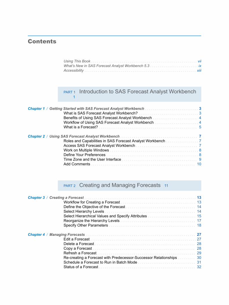
Using This Book . . . . . . . . . . . . . . . . . . . . . . . . . . . . . . . . . . . . . . . . . . . . . . . . . . . . . . . viiWhat’s New in SAS Forecast Analyst Workbench 5.3 . . . . . . . . . . . . . . . . . . . . . . . . . ixAccessibility . . . . . . . . . . . . . . . . . . . . . . . . . . . . . . . . . . . . . . . . . . . . . . . . . . . . . . . . . . xiii
PART 1 Introduction to SAS Forecast Analyst Workbench1
Chapter 1 / Getting Started with SAS Forecast Analyst Workbench . . . . . . . . . . . . . . . . . . . . . . . . . . . . 3What is SAS Forecast Analyst Workbench? . . . . . . . . . . . . . . . . . . . . . . . . . . . . . . . 3Benefits of Using SAS Forecast Analyst Workbench . . . . . . . . . . . . . . . . . . . . . . . 4Workflow of Using SAS Forecast Analyst Workbench . . . . . . . . . . . . . . . . . . . . . . . 4What is a Forecast? . . . . . . . . . . . . . . . . . . . . . . . . . . . . . . . . . . . . . . . . . . . . . . . . . . . 5
Chapter 2 / Using SAS Forecast Analyst Workbench . . . . . . . . . . . . . . . . . . . . . . . . . . . . . . . . . . . . . . . . 7Roles and Capabilities in SAS Forecast Analyst Workbench . . . . . . . . . . . . . . . . . 7Access SAS Forecast Analyst Workbench . . . . . . . . . . . . . . . . . . . . . . . . . . . . . . . . 7Work on Multiple Windows . . . . . . . . . . . . . . . . . . . . . . . . . . . . . . . . . . . . . . . . . . . . . . 8Define Your Preferences . . . . . . . . . . . . . . . . . . . . . . . . . . . . . . . . . . . . . . . . . . . . . . . . 8Time Zone and the User Interface . . . . . . . . . . . . . . . . . . . . . . . . . . . . . . . . . . . . . . . 9Add Comments . . . . . . . . . . . . . . . . . . . . . . . . . . . . . . . . . . . . . . . . . . . . . . . . . . . . . . 10
PART 2 Creating and Managing Forecasts 11
Chapter 3 / Creating a Forecast . . . . . . . . . . . . . . . . . . . . . . . . . . . . . . . . . . . . . . . . . . . . . . . . . . . . . . . . . . 13Workflow for Creating a Forecast . . . . . . . . . . . . . . . . . . . . . . . . . . . . . . . . . . . . . . . 13Define the Objective of the Forecast . . . . . . . . . . . . . . . . . . . . . . . . . . . . . . . . . . . . 14Select Hierarchy Levels . . . . . . . . . . . . . . . . . . . . . . . . . . . . . . . . . . . . . . . . . . . . . . . 14Select Hierarchical Values and Specify Attributes . . . . . . . . . . . . . . . . . . . . . . . . . 15Reorganize the Hierarchy Levels . . . . . . . . . . . . . . . . . . . . . . . . . . . . . . . . . . . . . . . 17Specify Other Parameters . . . . . . . . . . . . . . . . . . . . . . . . . . . . . . . . . . . . . . . . . . . . . 18
Chapter 4 / Managing Forecasts . . . . . . . . . . . . . . . . . . . . . . . . . . . . . . . . . . . . . . . . . . . . . . . . . . . . . . . . . 27Edit a Forecast . . . . . . . . . . . . . . . . . . . . . . . . . . . . . . . . . . . . . . . . . . . . . . . . . . . . . . . 27Delete a Forecast . . . . . . . . . . . . . . . . . . . . . . . . . . . . . . . . . . . . . . . . . . . . . . . . . . . . 28Copy a Forecast . . . . . . . . . . . . . . . . . . . . . . . . . . . . . . . . . . . . . . . . . . . . . . . . . . . . . 28Refresh a Forecast . . . . . . . . . . . . . . . . . . . . . . . . . . . . . . . . . . . . . . . . . . . . . . . . . . . 29Re-creating a Forecast with Predecessor-Successor Relationships . . . . . . . . . 30Schedule a Forecast to Run in Batch Mode . . . . . . . . . . . . . . . . . . . . . . . . . . . . . . 31Status of a Forecast . . . . . . . . . . . . . . . . . . . . . . . . . . . . . . . . . . . . . . . . . . . . . . . . . . 32

PART 3 Generating Predicted Values 35
Chapter 5 / Workflow for Generating Predicted Values . . . . . . . . . . . . . . . . . . . . . . . . . . . . . . . . . . . . . . 37Workflow for Generating Predicted Values . . . . . . . . . . . . . . . . . . . . . . . . . . . . . . . 37Status of a Forecast and Tasks Permitted in the Model Management View . . . 39
Chapter 6 / Generating and Analyzing Predicted Values . . . . . . . . . . . . . . . . . . . . . . . . . . . . . . . . . . . . 41Select Time Series . . . . . . . . . . . . . . . . . . . . . . . . . . . . . . . . . . . . . . . . . . . . . . . . . . . 41Diagnose Forecasts . . . . . . . . . . . . . . . . . . . . . . . . . . . . . . . . . . . . . . . . . . . . . . . . . . 42Edit Parameters . . . . . . . . . . . . . . . . . . . . . . . . . . . . . . . . . . . . . . . . . . . . . . . . . . . . . . 43Select a Default Model . . . . . . . . . . . . . . . . . . . . . . . . . . . . . . . . . . . . . . . . . . . . . . . . 55Create a Modeling Project . . . . . . . . . . . . . . . . . . . . . . . . . . . . . . . . . . . . . . . . . . . . . 55Rediagnose a Forecast . . . . . . . . . . . . . . . . . . . . . . . . . . . . . . . . . . . . . . . . . . . . . . . 57Reconcile a Forecast . . . . . . . . . . . . . . . . . . . . . . . . . . . . . . . . . . . . . . . . . . . . . . . . . 57Accept a Forecast . . . . . . . . . . . . . . . . . . . . . . . . . . . . . . . . . . . . . . . . . . . . . . . . . . . . 59Rerun the Forecast . . . . . . . . . . . . . . . . . . . . . . . . . . . . . . . . . . . . . . . . . . . . . . . . . . . 59
Chapter 7 / Viewing Details of a Forecast . . . . . . . . . . . . . . . . . . . . . . . . . . . . . . . . . . . . . . . . . . . . . . . . . 61Perform Frequent Tasks Related to Model Management . . . . . . . . . . . . . . . . . . . 61View Information about Time Series . . . . . . . . . . . . . . . . . . . . . . . . . . . . . . . . . . . . . 62Filter the Time Series . . . . . . . . . . . . . . . . . . . . . . . . . . . . . . . . . . . . . . . . . . . . . . . . . 63View Information about Changed Time Series . . . . . . . . . . . . . . . . . . . . . . . . . . . . 64View Forecast Plots . . . . . . . . . . . . . . . . . . . . . . . . . . . . . . . . . . . . . . . . . . . . . . . . . . 64View Predicted Values and Summary Information for a Forecast . . . . . . . . . . . . 65View Model Information . . . . . . . . . . . . . . . . . . . . . . . . . . . . . . . . . . . . . . . . . . . . . . . 66View Information About Child Products . . . . . . . . . . . . . . . . . . . . . . . . . . . . . . . . . . 67View Future Values of Changed Time Series . . . . . . . . . . . . . . . . . . . . . . . . . . . . . 67
PART 4 Integrating Modeling Projects with SAS Forecast Studio 69
Chapter 8 / Introduction to Modeling Projects . . . . . . . . . . . . . . . . . . . . . . . . . . . . . . . . . . . . . . . . . . . . . 71About Modeling Projects . . . . . . . . . . . . . . . . . . . . . . . . . . . . . . . . . . . . . . . . . . . . . . 71Workflow for Modeling Projects . . . . . . . . . . . . . . . . . . . . . . . . . . . . . . . . . . . . . . . . . 72View Predicted Values and Summary of a Modeling Project . . . . . . . . . . . . . . . . 73Status of Modeling Projects . . . . . . . . . . . . . . . . . . . . . . . . . . . . . . . . . . . . . . . . . . . . 75
Chapter 9 / Managing Modeling Projects . . . . . . . . . . . . . . . . . . . . . . . . . . . . . . . . . . . . . . . . . . . . . . . . . . 77Guidelines for Modeling Projects . . . . . . . . . . . . . . . . . . . . . . . . . . . . . . . . . . . . . . . 77Open SAS Forecast Studio . . . . . . . . . . . . . . . . . . . . . . . . . . . . . . . . . . . . . . . . . . . . 78Refresh a Modeling Project . . . . . . . . . . . . . . . . . . . . . . . . . . . . . . . . . . . . . . . . . . . . 78Promote a Modeling Project . . . . . . . . . . . . . . . . . . . . . . . . . . . . . . . . . . . . . . . . . . . 79Delete a Modeling Project . . . . . . . . . . . . . . . . . . . . . . . . . . . . . . . . . . . . . . . . . . . . . 79
PART 5 Forecasting a New Product 81
Chapter 10 / Forecasting a New Product . . . . . . . . . . . . . . . . . . . . . . . . . . . . . . . . . . . . . . . . . . . . . . . . . . 83Overview of Forecasting a New Product . . . . . . . . . . . . . . . . . . . . . . . . . . . . . . . . . 83
iv Contents

Workflow for Forecasting a New Product . . . . . . . . . . . . . . . . . . . . . . . . . . . . . . . . 84Create a New Product Forecast Project . . . . . . . . . . . . . . . . . . . . . . . . . . . . . . . . . 86View Details of a New Product Forecast Project . . . . . . . . . . . . . . . . . . . . . . . . . . 88Define Relationships and Candidate Products . . . . . . . . . . . . . . . . . . . . . . . . . . . . 88Select Candidate Products and Adjust Seasonality . . . . . . . . . . . . . . . . . . . . . . . . 89Select Surrogate Products . . . . . . . . . . . . . . . . . . . . . . . . . . . . . . . . . . . . . . . . . . . . . 91Select a Model . . . . . . . . . . . . . . . . . . . . . . . . . . . . . . . . . . . . . . . . . . . . . . . . . . . . . . . 92Review the Forecast . . . . . . . . . . . . . . . . . . . . . . . . . . . . . . . . . . . . . . . . . . . . . . . . . . 93Assigning New Product Forecast Projects to a Forecast . . . . . . . . . . . . . . . . . . . 94Delete a New Product Forecast Project . . . . . . . . . . . . . . . . . . . . . . . . . . . . . . . . . . 96Statuses of a New Product Forecast Project . . . . . . . . . . . . . . . . . . . . . . . . . . . . . 96
PART 6 Performing Custom Analyses 99
Chapter 11 / Performing Custom Analyses . . . . . . . . . . . . . . . . . . . . . . . . . . . . . . . . . . . . . . . . . . . . . . . 101Introduction to Performing Custom Analysis . . . . . . . . . . . . . . . . . . . . . . . . . . . . . 101Workflow for Using Custom Analysis . . . . . . . . . . . . . . . . . . . . . . . . . . . . . . . . . . . 101Create an Analysis . . . . . . . . . . . . . . . . . . . . . . . . . . . . . . . . . . . . . . . . . . . . . . . . . . 102Use the Three-Stage Modeling Analysis . . . . . . . . . . . . . . . . . . . . . . . . . . . . . . . . 103Edit an Analysis . . . . . . . . . . . . . . . . . . . . . . . . . . . . . . . . . . . . . . . . . . . . . . . . . . . . . 105Share an Analysis with Another User . . . . . . . . . . . . . . . . . . . . . . . . . . . . . . . . . . 105Delete an Analysis . . . . . . . . . . . . . . . . . . . . . . . . . . . . . . . . . . . . . . . . . . . . . . . . . . 106Explore the Output of the Analysis . . . . . . . . . . . . . . . . . . . . . . . . . . . . . . . . . . . . . 106
PART 7 Performing Collaboration Planning 107
Chapter 12 / Introduction to Collaboration Planning . . . . . . . . . . . . . . . . . . . . . . . . . . . . . . . . . . . . . . . 109What is Collaboration Planning? . . . . . . . . . . . . . . . . . . . . . . . . . . . . . . . . . . . . . . . 109Collaboration Planning Workflow . . . . . . . . . . . . . . . . . . . . . . . . . . . . . . . . . . . . . . 109
Chapter 13 / Performing Collaboration Planning . . . . . . . . . . . . . . . . . . . . . . . . . . . . . . . . . . . . . . . . . . 113Create a Plan . . . . . . . . . . . . . . . . . . . . . . . . . . . . . . . . . . . . . . . . . . . . . . . . . . . . . . . 113View Details of a Plan in the Collaboration Flow View . . . . . . . . . . . . . . . . . . . . 116Configure Analysis Variables . . . . . . . . . . . . . . . . . . . . . . . . . . . . . . . . . . . . . . . . . . 117Initiate the Collaboration . . . . . . . . . . . . . . . . . . . . . . . . . . . . . . . . . . . . . . . . . . . . . . 118Create Form Sets and Form Templates . . . . . . . . . . . . . . . . . . . . . . . . . . . . . . . . . 118Publish Form Sets . . . . . . . . . . . . . . . . . . . . . . . . . . . . . . . . . . . . . . . . . . . . . . . . . . . 120Obtain Input for Collaboration . . . . . . . . . . . . . . . . . . . . . . . . . . . . . . . . . . . . . . . . . 120Complete the Collaboration Process . . . . . . . . . . . . . . . . . . . . . . . . . . . . . . . . . . . 121Initialize the Collaboration Process . . . . . . . . . . . . . . . . . . . . . . . . . . . . . . . . . . . . 121
Chapter 14 / Managing Plans . . . . . . . . . . . . . . . . . . . . . . . . . . . . . . . . . . . . . . . . . . . . . . . . . . . . . . . . . . . 123Edit a Plan . . . . . . . . . . . . . . . . . . . . . . . . . . . . . . . . . . . . . . . . . . . . . . . . . . . . . . . . . 123Delete a Plan . . . . . . . . . . . . . . . . . . . . . . . . . . . . . . . . . . . . . . . . . . . . . . . . . . . . . . . 124Refresh a Plan . . . . . . . . . . . . . . . . . . . . . . . . . . . . . . . . . . . . . . . . . . . . . . . . . . . . . . 125Status of a Plan . . . . . . . . . . . . . . . . . . . . . . . . . . . . . . . . . . . . . . . . . . . . . . . . . . . . . 126
Contents v

PART 8 Analyzing Forecasts 129
Chapter 15 / Exploring Demand . . . . . . . . . . . . . . . . . . . . . . . . . . . . . . . . . . . . . . . . . . . . . . . . . . . . . . . . . 131Overview of Exploring Demand . . . . . . . . . . . . . . . . . . . . . . . . . . . . . . . . . . . . . . . 131Explore Demand . . . . . . . . . . . . . . . . . . . . . . . . . . . . . . . . . . . . . . . . . . . . . . . . . . . . 132
Chapter 16 / Performing Scenario Analysis . . . . . . . . . . . . . . . . . . . . . . . . . . . . . . . . . . . . . . . . . . . . . . 135Workflow for Scenario Analysis . . . . . . . . . . . . . . . . . . . . . . . . . . . . . . . . . . . . . . . 135Create a Scenario . . . . . . . . . . . . . . . . . . . . . . . . . . . . . . . . . . . . . . . . . . . . . . . . . . . 136Edit the Values of Independent Variables . . . . . . . . . . . . . . . . . . . . . . . . . . . . . . . 136Run and Save a Scenario . . . . . . . . . . . . . . . . . . . . . . . . . . . . . . . . . . . . . . . . . . . . 138Reset a Scenario . . . . . . . . . . . . . . . . . . . . . . . . . . . . . . . . . . . . . . . . . . . . . . . . . . . . 139Delete a Scenario . . . . . . . . . . . . . . . . . . . . . . . . . . . . . . . . . . . . . . . . . . . . . . . . . . . 139Export Scenario Values . . . . . . . . . . . . . . . . . . . . . . . . . . . . . . . . . . . . . . . . . . . . . . 139
PART 9 Administering Product Life Cycle in SAS Forecast Analyst Workbench 141
Chapter 17 / Managing the Life Cycle of Products . . . . . . . . . . . . . . . . . . . . . . . . . . . . . . . . . . . . . . . . . 143Product Life Cycle Workflow . . . . . . . . . . . . . . . . . . . . . . . . . . . . . . . . . . . . . . . . . . 143Search for Products . . . . . . . . . . . . . . . . . . . . . . . . . . . . . . . . . . . . . . . . . . . . . . . . . 144Specify Phase-in Details for a Product . . . . . . . . . . . . . . . . . . . . . . . . . . . . . . . . . 145Specify Phase-out Details for a Product . . . . . . . . . . . . . . . . . . . . . . . . . . . . . . . . 146Define a Successor Product . . . . . . . . . . . . . . . . . . . . . . . . . . . . . . . . . . . . . . . . . . 148Manage the Life Cycle for Multiple Products Simultaneously . . . . . . . . . . . . . . 150Generate Forecast Values for New Relationships . . . . . . . . . . . . . . . . . . . . . . . . 151Managing Life Cycle Details for a Product . . . . . . . . . . . . . . . . . . . . . . . . . . . . . . 152
PART 10 Generating Reports 157
Chapter 18 / Working with Reports . . . . . . . . . . . . . . . . . . . . . . . . . . . . . . . . . . . . . . . . . . . . . . . . . . . . . . 159About Reports . . . . . . . . . . . . . . . . . . . . . . . . . . . . . . . . . . . . . . . . . . . . . . . . . . . . . . 159View a Report . . . . . . . . . . . . . . . . . . . . . . . . . . . . . . . . . . . . . . . . . . . . . . . . . . . . . . 159Create a Report . . . . . . . . . . . . . . . . . . . . . . . . . . . . . . . . . . . . . . . . . . . . . . . . . . . . . 160
PART 11 Appendix 161
Appendix 1 / Performing Multi-Tier Causal Analysis . . . . . . . . . . . . . . . . . . . . . . . . . . . . . . . . . . . . . . . 163About Multi-Tiered Causal Analysis . . . . . . . . . . . . . . . . . . . . . . . . . . . . . . . . . . . . 163Perform Multi-Tiered Causal Analysis . . . . . . . . . . . . . . . . . . . . . . . . . . . . . . . . . . 163
Recommended Reading . . . . . . . . . . . . . . . . . . . . . . . . . . . . . . . . . . . . . . . . . . . . . 167Glossary . . . . . . . . . . . . . . . . . . . . . . . . . . . . . . . . . . . . . . . . . . . . . . . . . . . . . . . . . . . 169Index . . . . . . . . . . . . . . . . . . . . . . . . . . . . . . . . . . . . . . . . . . . . . . . . . . . . . . . . . . . . . . 179
vi Contents

Using This Book
Audience
SAS Forecast Analyst Workbench is designed for the following users:
n Administrators who are responsible for setting up and maintaining the application environment
n Data analysts who are responsible for data management
n Business users (including planners, analysts, and advanced analysts) who are responsible for analyzing the forecasted data and for making decisions based on that data
This document focuses on explaining the tasks that you can perform by using the SAS Forecast Analyst Workbench user interface. As a user of SAS Forecast Analyst Workbench, you might be assigned to a specific role, which determines the tasks that you can perform.
Prerequisites
You must satisfy the following prerequisites to use SAS Forecast Analyst Workbench:
n a user ID and password for logging on to SAS Forecast Analyst Workbench
n a supported web browser installed on your computer
n access to data sources or stored processes to obtain data
vii

viii Using This Book

Whatʼs New
What’s New in SAS Forecast Analyst Workbench 5.3
Overview
This chapter describes the new features and functionality that are added in the SAS Forecast Analyst Workbench 5.3 and in the first maintenance release of SAS Forecast Analyst Workbench 5.3.
SAS Forecast Analyst Workbench 5.3 contains new features that affect the following areas:
n enhancements in product lifecycle management
n additional capability for the Process Administrator role
n re-configuring data model
n general enhancements
Enhancements for the First Maintenance Release of SAS Forecast Analyst Workbench 5.3
The first maintenance release of SAS Forecast Analyst Workbench 5.3 contains the following enhancements:
Custom analysis Analysts can develop SAS Stored Processes that are custom analyses. These analyses can then be used by general users to analyze the data. This feature enables you to create analyses that use the solution’s analytic capabilities to more effectively meet your particular business requirements.
Connecting to SAS Viya
You can leverage the advanced capabilities of SAS Viya, a cloud-enabled platform, from within the first maintenance release of SAS Forecast Analyst Workbench 5.3. You can define the scope of your
ix

forecasting in the first maintenance release of SAS Forecast Analyst Workbench 5.3, which is based on SAS 9.4, export the data to SAS Viya, generate predicted values based on your custom analyses, and then import the data from SAS Viya into the first maintenance release of SAS Forecast Analyst Workbench 5.3.
Three-stage modeling
Three-stage modeling is an out-of-the-box analysis that can serve as a template for additional proprietary analysis. You can perform the three-stage modeling analysis on SAS 9.4 and on SAS Viya. When the analysis is performed on SAS Viya, the PROC TSMODEL and PROC REGSELECT are used.
Integrate the output of a custom analysis with downward processes
The output of a custom analysis can be integrated with the downward processes of supply-chain management. You can integrate the output of custom analysis with SAS Collaboration Planning Workbench for collaboration planning and with SAS Inventory Optimization Workbench for optimizing the inventory.
Disaggregate predicted values
You can write custom code that disaggregates the predicted values of a dimension hierarchy from a higher level to a lower level. Similarly, you can also write custom code to disaggregate the predicted values from any time granularity to the DAY level.
Enhancements in Product Lifecycle Management
The following enhancements in the product lifecycle management enable planners to define the phase-in relationships, phase-out relationships and successor relationships easily:
n changes in the user interface simplify the process of defining these relationships
n only relevant relationships are available for selection when you are defining these relationships
n surrogate forecasts are generated automatically for new phase-in relationships (previously you needed to define act-like relationships)
n you can now include the following types of information when data that is related to product life cycles is loaded to SAS Forecast Analyst Workbench through SAS Data Integration Studio:
o relationships containing the temporary phase-out dates
o relationships that are defined at a higher level
For example, suppose product A is going to be introduced at all stores in Los Angeles. In this case, instead of loading all individual relationships for product A with each store in Los Angeles, you can define and load a relationship for product A in Los Angeles.
x What’s New in SAS Forecast Analyst Workbench 5.3

Additional Capability to the Process Administrator Role
The Process Administrator can now monitor forecasts, modeling projects, new product forecast projects, and plans that are created by other users. The Process Administrators can use this capability to perform administrative tasks (such as deleting a forecast in the absence of its owner).
Re-Configuring Your Data Model
As your business requirements change, you might want to reconsider your goals and predict a different key performance indicator (KPI). You can now add a KPI to SAS Forecast Analyst Workbench.
Similarly, you can also add an independent variable to your deployment. You can use an already existing independent variable or you can add a new independent variable. For example, you can add Fuel as an independent variable.
General Enhancements
In addition to the enhancements mentioned above, the following enhancements have also been made:
n forecasting and collaboration planning can be performed by using custom time intervals that are supported by SAS
n it is easier to assign a new product forecast project to a forecast
n duplicate data from the Scratch library is removed in order to improve performance
n forecasted values of a new time series are automatically added to the forecast after they become available to the forecast
For example, suppose you create a forecast to predict demand values for a DSLR category of cameras. Then, a new camera, DSLR700i, is launched. If you use the user interface to re-create or refresh the forecast that you created for DSLR cameras, that forecast now contains the forecasted values for the DSLR700i camera model.
General Enhancements xi

xii What’s New in SAS Forecast Analyst Workbench 5.3

AccessibilityFor information about the accessibility of this product, see Accessibility Features of SAS Forecast Analyst Workbench 5.3 at support.sas.com.
xiii

xiv What’s New in SAS Forecast Analyst Workbench 5.3

Part 1Introduction to SAS Forecast Analyst Workbench
Chapter 1Getting Started with SAS Forecast Analyst Workbench . . . . . . . . . . . . . . . . . 3
Chapter 2Using SAS Forecast Analyst Workbench . . . . . . . . . . . . . . . . . . . . . . . . . . . . . 7
1

2

1
Getting Started with SAS Forecast Analyst Workbench
What is SAS Forecast Analyst Workbench? . . . . . . . . . . . . . . . . . . . . . . . . . . . . . . . . . . 3
Benefits of Using SAS Forecast Analyst Workbench . . . . . . . . . . . . . . . . . . . . . . . . . 4Potential for Higher Profits . . . . . . . . . . . . . . . . . . . . . . . . . . . . . . . . . . . . . . . . . . . . . . . . . . 4Better Insights . . . . . . . . . . . . . . . . . . . . . . . . . . . . . . . . . . . . . . . . . . . . . . . . . . . . . . . . . . . . . 4Improved Relations . . . . . . . . . . . . . . . . . . . . . . . . . . . . . . . . . . . . . . . . . . . . . . . . . . . . . . . . 4
Workflow of Using SAS Forecast Analyst Workbench . . . . . . . . . . . . . . . . . . . . . . . . 4
What is a Forecast? . . . . . . . . . . . . . . . . . . . . . . . . . . . . . . . . . . . . . . . . . . . . . . . . . . . . . . . . . . 5
What is SAS Forecast Analyst Workbench?
SAS Forecast Analyst Workbench is the demand planning module of the SAS for Demand-Driven Planning and Optimization suite. SAS Forecast Analyst Workbench helps planners and analysts track, monitor, and predict the demand for products and services. Whether you are operating your business within a country or across countries, you will find that SAS Forecast Analyst Workbench is an incredibly easy and powerful tool to use. SAS Forecast Analyst Workbench helps organizations gain instant visibility and understanding of the demand for their products without needing to rely on personal judgments.
SAS Forecast Analyst Workbench is empowered with the capabilities of SAS solutions—analytics, data integration, and business intelligence. SAS Forecast Analyst Workbench enables your organization to perform the following tasks:
n sense demand signals through the synchronization of internal and external data
n shape demand by using advanced analytics
n predict demand to create a more accurate, unconstrained demand forecast
Depending on the license that your organization has purchased, you can use the Collaboration module of SAS Forecast Analyst Workbench. (See Chapter 12, “Introduction to Collaboration Planning,” on page 109.)
3

Benefits of Using SAS Forecast Analyst Workbench
Potential for Higher Profits
Organizations benefit from more effective downstream planning due to improved demand forecasting results that anticipate unconstrained demand more accurately. More effective downstream planning includes the following benefits:
n a reduction in customer stock orders and retailer shelving
n a significant reduction in customer back orders
n a reduction in the carrying costs for finished goods inventory
n consistently high levels of customer service, which results in high customer retention (due to having the right product at the right time)
Better Insights
Due to the systematic workflow of SAS Forecast Analyst Workbench, collaboration between stakeholders within the organization improves. This improved collaboration leads to a better understanding of what drives profitability, which results in tighter budget control and more efficient allocation of marketing investment. This collaboration also results in a better understanding of products, customers, and market profitability.
Improved Relations
As all the internal stakeholders in the process begin to collaborate, they become more tightly aligned. This closeness enables quality collaboration among sales, marketing, finance, and operations planning. The building of quality relationships translates into stronger network integration, which helps minimize the pressures of market dynamics that surround your organization’s brand and products.
Workflow of Using SAS Forecast Analyst Workbench
After you log on to SAS Forecast Analyst Workbench, you can perform the following high-level series of tasks to generate the forecasted values:
1 Create a forecast.
Create a forecast that contains the key performance indicate for which you want to generate the forecasted values. You can also select dimensions, hierarchies, hierarchical values, and other information in a forecast.
2 Diagnose the forecast in order to generate the forecasted values.
4 Chapter 1 / Getting Started with SAS Forecast Analyst Workbench
You can specify the statistical parameters, reconcile the forecast, and perform various tasks (including creating a modeling project) on a forecast until the forecasted values are satisfactory.
3 Accept the forecast.
After the forecasted values are satisfactory, you can accept the forecast in order to apply the selected model to the forecast.
4 (Optional) Perform custom analysis on the forecast.
When you want to improve the quality of the forecast or you want to use custom methods of forecasting that better meet your business requirements, SAS consultants and analysts can write SAS Stored Processes as custom analyses. These custom analyses can then be used to generate predicted values.
5 (Optional) Perform new product forecasting.
If portfolio of products contains new products, you can use New Products workspace to predict the forecasted values of the new products, and then include those forecasted values in the forecast.
6 (Optional) Perform collaboration planning.
Perform collaboration planning in order to obtain inputs from all stakeholders within the organization on the unconstrained demand forecast. The inputs that are obtained from stakeholders can be included in the forecast.
7 Refresh the forecast.
Refresh the forecast in order to make the periodical data available to the forecast.
8 (Optional) Customize SAS Forecast Analyst Workbench.
The customizing options that are available in SAS Forecast Analyst Workbench enable you to generate the predicted values more accurately for your situation. For more information about understanding customizing options, see SAS Forecast Analyst Workbench: Administrator’s Guide.
What is a Forecast?
A forecast is the scope of the forecasting and planning activities. A forecast contains the following attributes:
n objective or type of the forecast that defines the planning purpose (for example, operational forecast)
n key performance indicator (KPI), which depends on the type of forecast that you choose (for example, demand)
n dimensions for which you want to forecast (for example, product or store location)
n hierarchy levels for each of the selected dimensions at which you might want to analyze the KPI
n hierarchy values for each of the selected hierarchy levels
What is a Forecast? 5

n information about the bill of material
n factors that impact or influence the planning variables, such as independent variables and events
The status of a forecast enables you to maintain a consistent and collaborative workflow within various departments of your organization. You can run a forecast in batch mode to periodically update the historical and predicted values.
6 Chapter 1 / Getting Started with SAS Forecast Analyst Workbench

2
Using SAS Forecast Analyst Workbench
Roles and Capabilities in SAS Forecast Analyst Workbench . . . . . . . . . . . . . . . . . . 7
Access SAS Forecast Analyst Workbench . . . . . . . . . . . . . . . . . . . . . . . . . . . . . . . . . . . 7Access SAS Forecast Analyst Workbench . . . . . . . . . . . . . . . . . . . . . . . . . . . . . . . . . . . 7
Work on Multiple Windows . . . . . . . . . . . . . . . . . . . . . . . . . . . . . . . . . . . . . . . . . . . . . . . . . . . 8
Define Your Preferences . . . . . . . . . . . . . . . . . . . . . . . . . . . . . . . . . . . . . . . . . . . . . . . . . . . . . 8
Time Zone and the User Interface . . . . . . . . . . . . . . . . . . . . . . . . . . . . . . . . . . . . . . . . . . . . 9
Add Comments . . . . . . . . . . . . . . . . . . . . . . . . . . . . . . . . . . . . . . . . . . . . . . . . . . . . . . . . . . . . . 10
Roles and Capabilities in SAS Forecast Analyst Workbench
SAS Forecast Analyst Workbench is shipped with three predefined roles: Planner, Forecast Analyst, and Process Administrator. Depending on the role that is assigned to you, you can view the hierarchy levels and their values.
Using SAS Management Console, an administrator can modify the roles and specify the capabilities that meet the guidelines for your organization. If you have questions about your assigned roles, contact your administrator.
Based on the role that is assigned to you, you can view the features on the user interface. For example, a planner can perform collaboration planning while a forecast analyst can apply various models to a forecast.
Access SAS Forecast Analyst Workbench
Access SAS Forecast Analyst Workbench
Log on to the user interface of SAS Forecast Analyst Workbench by entering the URL that is supplied by your administrator in the browser. For example, you might enter http://server01.abc.com/SASForecastAnalystWorkbench/.
7

Use various components of the SAS Forecast Analyst Workbench user interface to perform your tasks. The components, such as various panes, data tables, toolbars, views, help you achieve the goal of predicting future values.
The properties pane of a view displays the detailed information of the object that is selected in the view. For example, the Properties pane in the Forecasts category displays the detailed information of the selected forecast.
Work on Multiple Windows
Use the Tile pane to view the objects that you have opened. You can work on multiple windows at a time. The Tiles pane enables you compare definitions of various objects such as tables, and so on. For example, you can compare the predicted values of two forecasts in the Model Management view in separate windows. You can also use this feature to work on multiple objects together.
To work on multiple windows:
1 From the list that is displayed in the respective workspace, select the object that you want to open.
2 On the toolbar, click the menu, and then select Send to Tile Pane.
3 Repeat steps 1 and 2 for the other objects.
4 In the Tile pane, hold down the Ctrl key and select the objects that you want to view. Each object opens in a separate window.
Define Your Preferences
You can define the global preferences for all the SAS products that you are working with. You can also define preferences specifically for SAS Forecast Analyst Workbench.
To define preferences:
1 Select File Preferences. The Preferences window appears. The left pane is the category pane. The name of the right pane changes depending on the option that you select in the category pane.
2 In the category pane, click Global Preferences, and then define the global preferences.
The following table describes the fields in the Global Preferences pane.
Table 2.1 Fields in the Global Preferences Pane
Field Description
User locale Select a user locale from the list to specify the geographic region, language, and conventions. This setting might also apply to some SAS web applications that are not displayed with the Adobe Flash player.
8 Chapter 2 / Using SAS Forecast Analyst Workbench

Field Description
Theme Select a theme from the list. The theme specifies the collection of colors, graphics, fonts, and effects that appear in the application.
Invert application colors
Select this check box to invert all of the colors in the application window, including text and graphical elements. You can also temporarily invert or revert the colors for an individual application session by pressing Ctrl+~.
3 In the category pane, expand SAS Forecast Analyst Workbench, and click General.
4 Define the general preferences.
The following table describes the fields of the General pane.
Table 2.2 Fields in the General Pane
Field Description
Open application using this workspace
Select a workspace that will appear as the default workspace when you log on to SAS Forecast Analyst Workbench.
Both icons and labels
Select this option to view both icons and labels on the user interface.
Icons only Select this option to view only icons on the user interface.
Labels only Select this option to view only labels on the user interface.
5 Click OK.
Time Zone and the User Interface
You can access the user interface of SAS Forecast Analyst Workbench by using a browser. SAS Forecast Analyst Workbench does not perform the time zone conversion automatically if the SAS Forecast Analyst Workbench server and browser are located in different time zones. Therefore, the demand that you see for a date and time on the user interface is the demand for that particular server date and time. You must perform the time zone conversion manually to determine the exact demand in your time zone.
Time Zone and the User Interface 9

Add Comments
You can add comments to the selected object by using the Comments Manager pane. Comment include information that is specific to that object and that you want to share and discuss with others. You can add a comment to a forecast, modeling project, and plan.
You can also perform the following tasks in the Comments Manager pane:
n create a topic
You can enter a subject and description for the new topic. You can select the priority of the topic and attach the important files to the comment.
n reply to a topic
n search for a topic to comment on
To add a comment:
1 Select an object.
You can select a forecast, modeling project, or a plan.
2 In the Comments Manager pane, enter the topic name and description.
3 (Optional) Click to attach a file to the comment.
4 Click Post.
10 Chapter 2 / Using SAS Forecast Analyst Workbench

Part 2Creating and Managing Forecasts
Chapter 3Creating a Forecast . . . . . . . . . . . . . . . . . . . . . . . . . . . . . . . . . . . . . . . . . . . . . . . 13
Chapter 4Managing Forecasts . . . . . . . . . . . . . . . . . . . . . . . . . . . . . . . . . . . . . . . . . . . . . . 27
11

12
3
Creating a Forecast
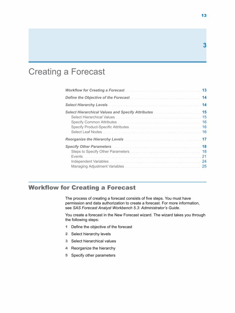
Workflow for Creating a Forecast . . . . . . . . . . . . . . . . . . . . . . . . . . . . . . . . . . . . . . . . . . . 13
Define the Objective of the Forecast . . . . . . . . . . . . . . . . . . . . . . . . . . . . . . . . . . . . . . . . 14
Select Hierarchy Levels . . . . . . . . . . . . . . . . . . . . . . . . . . . . . . . . . . . . . . . . . . . . . . . . . . . . . 14
Select Hierarchical Values and Specify Attributes . . . . . . . . . . . . . . . . . . . . . . . . . . . 15Select Hierarchical Values . . . . . . . . . . . . . . . . . . . . . . . . . . . . . . . . . . . . . . . . . . . . . . . . . 15Specify Common Attributes . . . . . . . . . . . . . . . . . . . . . . . . . . . . . . . . . . . . . . . . . . . . . . . 16Specify Product-Specific Attributes . . . . . . . . . . . . . . . . . . . . . . . . . . . . . . . . . . . . . . . . . 16Select Leaf Nodes . . . . . . . . . . . . . . . . . . . . . . . . . . . . . . . . . . . . . . . . . . . . . . . . . . . . . . . . 16
Reorganize the Hierarchy Levels . . . . . . . . . . . . . . . . . . . . . . . . . . . . . . . . . . . . . . . . . . . . 17
Specify Other Parameters . . . . . . . . . . . . . . . . . . . . . . . . . . . . . . . . . . . . . . . . . . . . . . . . . . . 18Steps to Specify Other Parameters . . . . . . . . . . . . . . . . . . . . . . . . . . . . . . . . . . . . . . . . 18Events . . . . . . . . . . . . . . . . . . . . . . . . . . . . . . . . . . . . . . . . . . . . . . . . . . . . . . . . . . . . . . . . . . . 21Independent Variables . . . . . . . . . . . . . . . . . . . . . . . . . . . . . . . . . . . . . . . . . . . . . . . . . . . . 24Managing Adjustment Variables . . . . . . . . . . . . . . . . . . . . . . . . . . . . . . . . . . . . . . . . . . . 25
Workflow for Creating a Forecast
The process of creating a forecast consists of five steps. You must have permission and data authorization to create a forecast. For more information, see SAS Forecast Analyst Workbench 5.3: Administrator’s Guide.
You create a forecast in the New Forecast wizard. The wizard takes you through the following steps:
1 Define the objective of the forecast
2 Select hierarchy levels
3 Select hierarchical values
4 Reorganize the hierarchy
5 Specify other parameters
13

Define the Objective of the Forecast
A forecast consists of its name, its objective, and its dimensions. You define the objective for the forecast by specifying the key performance indicator (KPI). For example, you can define Demand as the KPI in order to use historical demand for predicting the future demand.
To define the objective of the forecast:
1 In the Forecast Plans workspace, click . The New Forecast wizard appears.
2 Enter a name for the forecast.
Note: The forecast name must be unique and must be a valid SAS name. For more information about SAS naming conventions, see SAS Language Reference: Concepts at support.sas.com.
3 Enter a short description for the forecast.
4 In the Type list, select the forecast type. A forecast type defines the objective of your forecast.
Note: The key performance indicators in the KPI list depend on the forecast type that you select.
5 In the KPI list, select the key performance indicator. Key performance indicator is the dependent variable that you want to forecast.
Note: The dimensions that you see in the Available items section depend on the KPI that you select.
6 In the Available items section, select a dimension and click . The selected dimension appears in the Selected items section.
7 Click Next to continue. The Select Hierarchy Levels page appears.
Select Hierarchy Levels
On the Select Hierarchy Levels page, choose the hierarchy levels that you want to include in the forecast. You must specify hierarchy levels for all dimensions that you have selected.
To select hierarchy levels:
1 In the Dimension list, select a dimension. For example, you can select PRODUCT to predict the demand for your products.
2 In the Available items section, select the hierarchy level and click . The selected hierarchy level appears in the Selected items section.
Note: You cannot select only the lowest-level leaf node. You must select the parent node of the lowest-level leaf node in the hierarchy.
14 Chapter 3 / Creating a Forecast

3 Repeat steps 1 and 2 for all the dimensions.
4 Click Next to continue.
Select Hierarchical Values and Specify Attributes
Select Hierarchical Values
You must choose the hierarchical values for all the dimensions that you included in the forecast. You can also specify common attributes and product-specific attributes (also called product specifications) to further filter the data.
To select hierarchical values:
1 In the Dimension list, select a dimension.
2 In the Available items section, select the hierarchical value that you want to include. The hierarchical values are arranged in a tree structure. You can expand and collapse the hierarchy to select the values.
3 Click . The selected hierarchical values appear in the Selected items section.
Note: You must select valid hierarchy values.
4 Repeat steps 1 through 3 for all the dimensions.
5 (Optional) Click Common attributes to define the common attributes.
For more information about defining common attributes, see “Specify Common Attributes” on page 16.
Note: This link is available only if common attributes are defined for the selected hierarchical values.
6 (Optional) Click Product-specific attributes to define the attributes that are specific to a product.
For more information about defining product-specific attributes, see “Specify Product-Specific Attributes” on page 16.
Note: This link is available only if product-specific attributes are defined for the selected hierarchical values.
7 (Optional) Click Select leaf nodes to define the leaf nodes for the selected dimension.
For more information, see “Select Leaf Nodes” on page 16.
Note: This link is available only when the parent node of the lowest-level leaf node is selected and the forecast contains lowest leaf-level nodes.
8 Click Next to continue.
Select Hierarchical Values and Specify Attributes 15

Specify Common Attributes
You can specify additional criteria that are common among all members in a dimension in order to filter the data.
To specify the common attributes:
1 On the Select Hierarchical Values page of the New Forecast wizard, select a hierarchical value in the Selected items section.
2 Click Common attributes. The Common Attributes window appears.
3 Specify the parameters and click OK. For example, you can specify to forecast the demand for all products that are manufactured in the Seoul, South Korea plant and set the life cycle stage to MATURE.
When you specify attributes at different levels, SAS Forecast Analyst Workbench filters the data at the top-most level first. In other words, SAS Forecast Analyst Workbench filters the data from the top level to the bottom level when the following conditions are true:
n the data is arranged in a hierarchy
n the attributes that are defined at the highest level are different from the attributes that are defined at lower levels in the hierarchy
For example, SAS Forecast Analyst Workbench filters all red shirts first and then filters by size when shirt color is defined at the highest level in the hierarchy.
The attributes are specified at the selected hierarchy level.
Specify Product-Specific Attributes
You can specify additional criteria that are specific to a product or to a group of products under one category. For example, you can specify to forecast the demand for all television units that are based on LED technology and that have a 59-inch screen.
To specify product-specific attributes:
1 On the Select Hierarchical Values page of the New Forecast wizard, select a hierarchical value in the Available items section.
Note: You can set the attributes that are specific to products.
2 Click Product-specific attributes. The Specific Attributes window appears.
Note: This link is not available when the selected hierarchy node does not contain product-specific attributes.
3 Define the parameters and click OK.
The products are selected based on the specified attributes.
Select Leaf Nodes
By default, all leaf nodes are included in a forecast.
To select the leaf nodes:
16 Chapter 3 / Creating a Forecast

1 In the Dimension list on the Select Hierarchical Values page of the New Forecast wizard, select a dimension.
2 In the Selected items section, expand the hierarchy, and select the lower-level node.
3 Click the Select Leaf nodes link. The Select Node window appears.
4 Select the nodes that you want to include for forecasting, and click OK.
Click the Select all nodes option in order to include any new leaf nodes (that might be added to the node that is above the leaf node) to the forecast in the incremental run. These new leaf nodes that are added to the forecast are considered when you refresh and re-create the forecast.
Click the Select specific nodes option to add only specified leaf nodes to the forecast. The new leaf nodes (that might be added to node that is above the leaf node) are not added to the forecast.
Reorganize the Hierarchy Levels
To reorganize the hierarchy levels:
1 In the Hierarchy Level column, select a level and click or .
You reorganize the hierarchy based on your purpose. For example, if you want to forecast the demand for all the products in a store, move the Product level to be immediately below the Store Location level.
You cannot change the order of the hierarchy levels within a dimension. For example, for the Location dimension, you cannot move the States hierarchy level above the Regions hierarchy level. You can change the order of the hierarchy levels across dimensions.
2 In the Forecast Leaf Level column, click the lowest level up to which the forecasting process must run.
By defining the forecast-leaf-level node, you specify the level up to which the forecasting process must generate the forecasting values. For all levels below the forecast leaf level, SAS Forecast Analyst Workbench uses the disaggregation method to generate the predicted values.
3 In the Reconciliation Level column, select the level at which the reconciliation method must start.
Note: You cannot select a reconciliation level that is below the forecast leaf level that you selected.
By defining the reconciliation level, you specify the level at which the process of reconciliation must start. Based on the reconciliation level, SAS Forecast Analyst Workbench automatically selects one of the following reconciliation methods: bottom-up, middle-out, or top-down. If the reconciliation level that you selected is the same as that of forecast leaf level, SAS Forecast Analyst Workbench uses the bottom-up method for reconciliation. If you select the highest level, SAS Forecast Analyst Workbench uses the top-down method for reconciliation. For all other levels, SAS Forecast Analyst Workbench uses the middle-out method for reconciliation.
Reorganize the Hierarchy Levels 17
4 In the Periodicity list, select the periodicity.
The periodicity defines the forecasting interval, which is the frequency at which the data is forecasted.
5 In the Number of periods of historical data field, enter the number of periods of historical data that the forecasting process must include for generating forecast results.
6 In the Number of periods in forecast horizon field, enter the number of periods for which you want to generate forecast results.
7 In the Least number of periods to use statistical forecast results field, enter the least number of periods that the forecasting process should consider in order to use statistical forecast results. If the number of periods for any times series is less than the specified value, SAS Forecast Analyst Workbench automatically uses the predicted values of another time series that is more similar to the selected time series.
8 Click Next to continue, or click Finish.
If you click Finish, the status of the forecast becomes Creating. If the data is present in accordance with the parameters that you specified, the status of the forecast changes to Created.
Specify Other Parameters
Steps to Specify Other Parameters
On the Specify Other Parameters page, you can specify product chaining settings, events, and independent variables in order to generate forecast results.
To specify other parameters:
1 On the Product Chaining tab, specify bill of material information.
You can explode the bill of material of the combined products while the forecasting results are being generated. When you explode the bill of material, the forecasting process generates the predicted values of child products separately. If you do not explode the bill of material, the forecasting process considers the combined products as a single product, and then generates the forecast result. The Explore bill of materials list is available when the forecast contains combined products.
Note: The Product Chaining tab is available only if you selected the Product dimension when you created the forecast.
2 On the Events tab, select the events that you want to apply to all time series that are included in the forecast, and select the method of event usage.
The following table describes the fields available on the Events tab.
18 Chapter 3 / Creating a Forecast

Table 3.1 Fields on the Events Tab
Button or Field Description
Name The name of the event.
Description The description of the event.
Type The type of the event.
Event Usage Select an option from the list to specify how events must be used when the model is generated. You can use one of the following options:n Select Do not use to exclude the event in the model.n Select Force use to include the event in the model, if
feasible. By default, this option is selected.n Select Try to use to include the event in the model (if
feasible) if the resulting model is stable and is an improvement over the simple model.
n Select Use if significant to include the event in the model (if feasible) if the resulting model is stable, is an improvement over the simple model, and if the event is significant.
Event Class The event class information.
Before Duration (In periods)
Specifies the applicability of the event to periods before the occurrence of the event. For example, suppose the event is BOXING, it occurs on December 26, the Before Duration value is 2, and the periodicity is weekly. In this case, the event is applicable beginning on December 13.
After Duration (In periods)
Specifies the applicability of the event to periods after the occurrence of the event. For example, suppose the event is BOXING, it occurs on December 26, the After Duration value is 1, and the periodicity is weekly. In this case, the event is applicable until January 01.
Event Recurrence
For more information about event recurrence, see Table 3.6 on page 22.
Event Occurrence
The key name of the event, which indicates when it should occur. For example, if the key name is BOXING, the event occurs on December 26. If the key name is NEWYEAR, the event occurs on January 1.
For more information about event occurrence, see Table 3.7 on page 23.
Starting Date The starting date of the event.
Ending Date The end date of the event.
For more information about events, see “Events” on page 21.
3 On the Independent Variables tab, select the independent variables and the method of aggregation.
Specify Other Parameters 19

For more information about independent variables, see “Independent Variables” on page 24.
Note: Independent variables that are used as adjustment variables can no longer be included as independent variables.
TIP If only one transactional data point is present for every time period, do not select the STD aggregation method.
4 (Optional) Select the adjustment variables along with the independent variables.
To manage adjustment variables:
a On the Independent Variables tab, click Adjustments. The Adjustments window appears.
b Enter the appropriate information in each field. The following table describes each field.
Table 3.2 Fields in the Adjustments Window
Field Description
Adjusting Variable
Displays the name of the adjustment variable. Select the adjustment variable to apply it.
Note: The Adjustments window displays the variables that are not selected as independent variables.
Description Enter the description for the selected adjustment variable.
Aggregation Method
Select the aggregation method for the selected adjustment variable.
Pre-operation Select an option from the list for pre-operation.
Post-operation
Select an option from the list for post-operation.
c Select the order of the adjustment variables by using the or buttons.
You prioritize or order the adjustment variables to calculate the predicted values.
d Click OK.
For more information about adjustment variables, see “Managing Adjustment Variables” on page 25.
5 Click Finish.
The forecast is created in the Creating state. After the forecast is completed, the status of the forecast changes to Created.
20 Chapter 3 / Creating a Forecast
Events
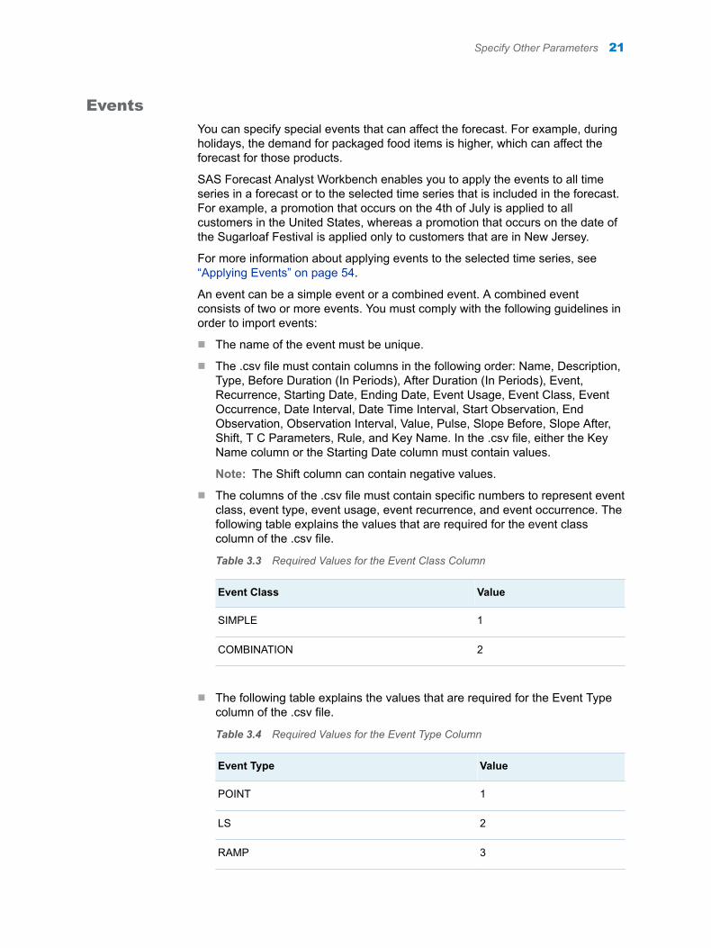
You can specify special events that can affect the forecast. For example, during holidays, the demand for packaged food items is higher, which can affect the forecast for those products.
SAS Forecast Analyst Workbench enables you to apply the events to all time series in a forecast or to the selected time series that is included in the forecast. For example, a promotion that occurs on the 4th of July is applied to all customers in the United States, whereas a promotion that occurs on the date of the Sugarloaf Festival is applied only to customers that are in New Jersey.
For more information about applying events to the selected time series, see “Applying Events” on page 54.
An event can be a simple event or a combined event. A combined event consists of two or more events. You must comply with the following guidelines in order to import events:
n The name of the event must be unique.
n The .csv file must contain columns in the following order: Name, Description, Type, Before Duration (In Periods), After Duration (In Periods), Event, Recurrence, Starting Date, Ending Date, Event Usage, Event Class, Event Occurrence, Date Interval, Date Time Interval, Start Observation, End Observation, Observation Interval, Value, Pulse, Slope Before, Slope After, Shift, T C Parameters, Rule, and Key Name. In the .csv file, either the Key Name column or the Starting Date column must contain values.
Note: The Shift column can contain negative values.
n The columns of the .csv file must contain specific numbers to represent event class, event type, event usage, event recurrence, and event occurrence. The following table explains the values that are required for the event class column of the .csv file.
Table 3.3 Required Values for the Event Class Column
Event Class Value
SIMPLE 1
COMBINATION 2
n The following table explains the values that are required for the Event Type column of the .csv file.
Table 3.4 Required Values for the Event Type Column
Event Type Value
POINT 1
LS 2
RAMP 3
Specify Other Parameters 21
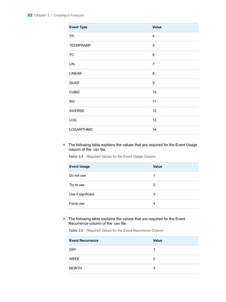
Event Type Value
TR 4
TEEMPRAMP 5
TC 6
LIN 7
LINEAR 8
QUAD 9
CUBIC 10
INV 11
INVERSE 12
LOG 13
LOGARITHMIC 14
n The following table explains the values that are required for the Event Usage column of the .csv file.
Table 3.5 Required Values for the Event Usage Column
Event Usage Value
Do not use 1
Try to use 2
Use if significant 3
Force use 4
n The following table explains the values that are required for the Event Recurrence column of the .csv file.
Table 3.6 Required Values for the Event Recurrence Column
Event Recurrence Value
DAY 1
WEEK 2
MONTH 3
22 Chapter 3 / Creating a Forecast

Event Recurrence Value
QTR 4
YEAR 5
Note: If you enter a value in the keyname field in the .csv file, then you do not need to enter a value in the Event Recurrence column or in the Starting Date column in the .csv file.
n The following table explains the values that are required for the Event Occurrence column of the .csv file.
Table 3.7 Required Values for the Event Occurrence Column
Event Occurrence Value
BOXING 1
CANADA 2
CANADAOBSERVED 3
CHRISTMAS 4
COLUMBUS 5
EASTER 6
FATHERS 7
HALLOWEEN 8
LABOR 9
MLK 10
MEMORIAL 11
MOTHERS 12
NEWYEAR 13
THANKSGIVING 14
THANKSGIVINGCANADA 15
USINDEPENDENCE 16
USPRESIDENTS 17
VALENTINES 18
VETERANS 19
Specify Other Parameters 23
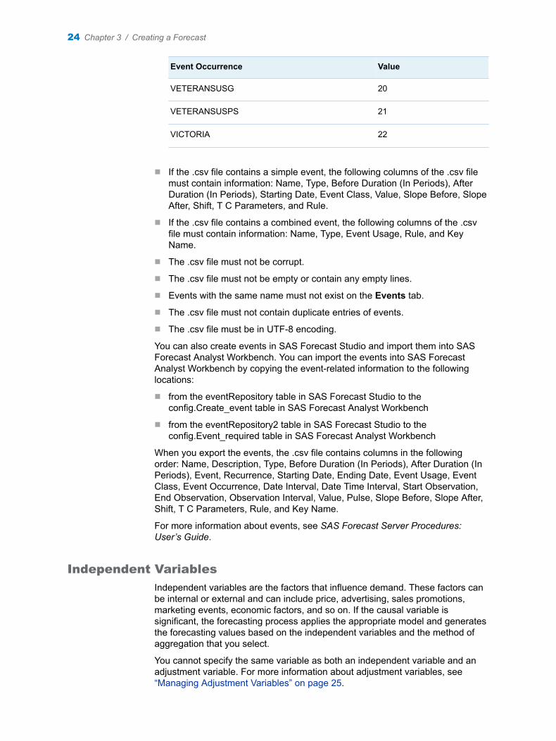
Event Occurrence Value
VETERANSUSG 20
VETERANSUSPS 21
VICTORIA 22
n If the .csv file contains a simple event, the following columns of the .csv file must contain information: Name, Type, Before Duration (In Periods), After Duration (In Periods), Starting Date, Event Class, Value, Slope Before, Slope After, Shift, T C Parameters, and Rule.
n If the .csv file contains a combined event, the following columns of the .csv file must contain information: Name, Type, Event Usage, Rule, and Key Name.
n The .csv file must not be corrupt.
n The .csv file must not be empty or contain any empty lines.
n Events with the same name must not exist on the Events tab.
n The .csv file must not contain duplicate entries of events.
n The .csv file must be in UTF-8 encoding.
You can also create events in SAS Forecast Studio and import them into SAS Forecast Analyst Workbench. You can import the events into SAS Forecast Analyst Workbench by copying the event-related information to the following locations:
n from the eventRepository table in SAS Forecast Studio to the config.Create_event table in SAS Forecast Analyst Workbench
n from the eventRepository2 table in SAS Forecast Studio to the config.Event_required table in SAS Forecast Analyst Workbench
When you export the events, the .csv file contains columns in the following order: Name, Description, Type, Before Duration (In Periods), After Duration (In Periods), Event, Recurrence, Starting Date, Ending Date, Event Usage, Event Class, Event Occurrence, Date Interval, Date Time Interval, Start Observation, End Observation, Observation Interval, Value, Pulse, Slope Before, Slope After, Shift, T C Parameters, Rule, and Key Name.
For more information about events, see SAS Forecast Server Procedures: User’s Guide.
Independent Variables
Independent variables are the factors that influence demand. These factors can be internal or external and can include price, advertising, sales promotions, marketing events, economic factors, and so on. If the causal variable is significant, the forecasting process applies the appropriate model and generates the forecasting values based on the independent variables and the method of aggregation that you select.
You cannot specify the same variable as both an independent variable and an adjustment variable. For more information about adjustment variables, see “Managing Adjustment Variables” on page 25.
24 Chapter 3 / Creating a Forecast

Managing Adjustment Variables
If systematic variations and deterministic components are included in time series data, you can specify an adjustment variable to identify the data that should be excluded before you perform a statistical analysis.
Using SAS Forecast Analyst Workbench, you can specify the adjustment variables in the following ways:
n before you generate the forecast
After the time-stamped data has been accumulated and interpreted, you might need to adjust the time series before you generate the forecast. By adjusting the time series for any known systematic variations or deterministic components, you can more easily identify and model the underlying time series process.
Examples of systematic adjustments are exchange rates, currency conversions, and trading days. Examples of deterministic adjustments are advanced bookings and reservations and contractual agreements.
n after you generate the forecast
You might need to adjust the statistical forecast in order to return the forecasts to the metric used in the original data.
Generally, the adjustments that you make before you generate the forecast and those that you make afterward are operations that are the inverse of each other.
Specify Other Parameters 25

26 Chapter 3 / Creating a Forecast

4
Managing Forecasts
Edit a Forecast . . . . . . . . . . . . . . . . . . . . . . . . . . . . . . . . . . . . . . . . . . . . . . . . . . . . . . . . . . . . . 27
Delete a Forecast . . . . . . . . . . . . . . . . . . . . . . . . . . . . . . . . . . . . . . . . . . . . . . . . . . . . . . . . . . . 28
Copy a Forecast . . . . . . . . . . . . . . . . . . . . . . . . . . . . . . . . . . . . . . . . . . . . . . . . . . . . . . . . . . . . 28
Refresh a Forecast . . . . . . . . . . . . . . . . . . . . . . . . . . . . . . . . . . . . . . . . . . . . . . . . . . . . . . . . . 29
Re-creating a Forecast with Predecessor-Successor Relationships . . . . . . . . . 30About Re-creating a Forecast with Predecessor-Successor Relationships . . . . 30Re-create a Forecast with Predecessor-Successor Relationships . . . . . . . . . . . . 31
Schedule a Forecast to Run in Batch Mode . . . . . . . . . . . . . . . . . . . . . . . . . . . . . . . . . 31
Status of a Forecast . . . . . . . . . . . . . . . . . . . . . . . . . . . . . . . . . . . . . . . . . . . . . . . . . . . . . . . . 32
Edit a Forecast
You can edit a forecast in order to modify your demand forecasting criteria. For example, you can include special events in the forecast.
Note: If you want to update all parameters of the forecast, you must create a new copy of the forecast and edit it. Fore more information about copying a forecast, see “Copy a Forecast” on page 28.
The following prerequisites apply:
n You must have permission to edit a forecast. For more information, contact your system administrator.
n The forecast status must be in one of the following states: Draft, Ready to create, Created, or Forecasted.
n If a modeling project is created for the forecast, the modeling project cannot be opened in SAS Forecast Studio.
To edit a forecast:
1 In the Forecast Plans workspace, click Forecasts. The Forecasts category appears. Select a forecast, and click . A message appears that informs you that the edit functionality is limited.
2 Click Yes. The Edit Forecast window appears.
3 Edit the information and click Finish.
27
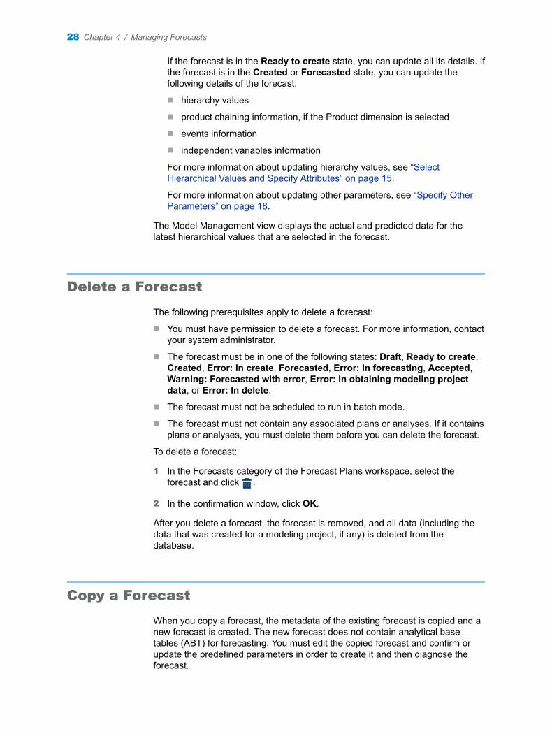
If the forecast is in the Ready to create state, you can update all its details. If the forecast is in the Created or Forecasted state, you can update the following details of the forecast:
n hierarchy values
n product chaining information, if the Product dimension is selected
n events information
n independent variables information
For more information about updating hierarchy values, see “Select Hierarchical Values and Specify Attributes” on page 15.
For more information about updating other parameters, see “Specify Other Parameters” on page 18.
The Model Management view displays the actual and predicted data for the latest hierarchical values that are selected in the forecast.
Delete a Forecast
The following prerequisites apply to delete a forecast:
n You must have permission to delete a forecast. For more information, contact your system administrator.
n The forecast must be in one of the following states: Draft, Ready to create, Created, Error: In create, Forecasted, Error: In forecasting, Accepted, Warning: Forecasted with error, Error: In obtaining modeling project data, or Error: In delete.
n The forecast must not be scheduled to run in batch mode.
n The forecast must not contain any associated plans or analyses. If it contains plans or analyses, you must delete them before you can delete the forecast.
To delete a forecast:
1 In the Forecasts category of the Forecast Plans workspace, select the forecast and click .
2 In the confirmation window, click OK.
After you delete a forecast, the forecast is removed, and all data (including the data that was created for a modeling project, if any) is deleted from the database.
Copy a Forecast
When you copy a forecast, the metadata of the existing forecast is copied and a new forecast is created. The new forecast does not contain analytical base tables (ABT) for forecasting. You must edit the copied forecast and confirm or update the predefined parameters in order to create it and then diagnose the forecast.
28 Chapter 4 / Managing Forecasts

The following prerequisites apply:
n You must have permission to copy a forecast. For more information, contact your system administrator.
n The forecast must be in one of the following states: Draft, Ready to create, Created, Forecasted, Error: In forecasting, Accepted, Error: In obtaining modeling project data, or Warning: Forecasted with error
n The forecast must not be scheduled to run in batch mode.
n You must have created the forecast that you want to copy.
To copy a forecast in order to use it as the basis for a new forecast:
1 In the Forecasts category of the Forecast Plans workspace, select a forecast, and click . The Copy Forecast window appears.
2 In the Name field, enter a name for the forecast and click OK. The application starts copying the metadata of the forecast, and a confirmation window appears.
3 Click OK. The application creates the forecast in the Ready to create state and displays it in the Forecasts list.
Now you can edit the parameters of the forecast.
4 In the Forecasts list, select the forecast that you copied, and click . The Edit Forecast window appears.
5 Update the information about the forecast.
For more information about updating the objectives and dimensions of the forecast, see “Define the Objective of the Forecast” on page 14.
For more information about updating the hierarchy levels of the forecast, see “Select Hierarchy Levels” on page 14.
For more information about updating the hierarchical values of the forecast, see “Select Hierarchical Values and Specify Attributes” on page 15.
For more information about reorganizing the hierarchy, see “Reorganize the Hierarchy Levels” on page 17.
For more information about updating other parameters, see “Specify Other Parameters” on page 18.
6 Click Finish.
The forecast is created with new parameters. Now you can apply different models to the forecast in the Model Management view.
Refresh a Forecast
When you refresh a forecast, incremental historical data is added to the forecast. If you selected the Select all nodes option while you were creating a forecast and you subsequently refresh the forecast, the new leaf nodes (that might be added during the incremental run to the node that is above the leaf node) are also included in the forecast.
Refresh a Forecast 29

The forecast must be in one of the following states: Created, Forecasted, Error: In forecasting, Accepted, or Warning: Forecasted with error.
To refresh a forecast:
1 If the GL_FORECAST_DATE parameter does not contain today() and you want to refresh the forecast on the current date or on a specific future date, enter that date for GL_FORECAST_DATE.
For more information about the GL_FORECAST_DATE parameter, see SAS Forecast Analyst Workbench 5.3: Administrator’s Guide.
2 In the Forecasts category of the Forecast Plans workspace, select a forecast, and click .
3 In the confirmation window, click Yes.
The selected forecast is refreshed and the new data is loaded into the forecast according to the periodicity and forecast start date settings. After you refresh a forecast, its status might change. The following table explains the possible status of a forecast when you refresh it.
Table 4.1 Status of a Forecast Before and After Refreshing
Status before the refresh Status after the refresh
Created Created
Error: In create Created (if the error is removed from the forecast)
Forecasted Forecasted
Accepted Forecasted
Warning: Forecasted with errors Forecasted (if the error is removed from the predicted values)
Error: In forecasting Forecasted (if the error is removed from the predicted values)
Re-creating a Forecast with Predecessor-Successor Relationships
About Re-creating a Forecast with Predecessor-Successor Relationships
Re-create a forecast in order to include the data for the latest relationships of predecessors and successors. You define these predecessor and successor relationships while you work with the life cycle of the products. For more information about managing product life cycle, see Chapter 17, “Managing the Life Cycle of Products,” on page 143.
30 Chapter 4 / Managing Forecasts

When a successor relationship is going to be introduced after the previous forecast date, SAS Forecast Analyst Workbench does not consider the predecessor-successor relationship. In order to consider the predecessor-successor relationship in the forecast, re-create the forecast so that historical data of the predecessor is considered in the prediction of the future values of the successor. For example, suppose product P1 is going to be succeeded by product S1 on 01 February. Also, the previous forecast date or horizon start date of the forecast that has monthly periodicity was 15 January. In this case, on 15 February, you click in order to add the historical data up to 31 January of product P1 to generate the forecasted data for product S1.
When you re-create the forecast, the new leaf level nodes (that might be added during the incremental run to the node that is above the leaf node) are also included in the forecast.
If the incremental historical data does not contain any predecessor-successor relationships, refresh the forecast. For more information about refreshing a forecast, see “Refresh a Forecast” on page 29.
Re-create a Forecast with Predecessor-Successor Relationships
To re-create the forecast with predecessor-successor relationships:
1 In the Forecast Plans workspace, click Forecasts. The Forecasts category appears.
2 Select a forecast, and click .
SAS Forecast Analyst Workbench starts including all time series that are related to product succession in the forecast and the status of the forecast becomes Created.
3 Click Diagnose in order to generate the forecasted values.
If the status of the forecast is other than Created, click Rediagnose.
Schedule a Forecast to Run in Batch Mode
After a forecast is scheduled to run in the batch mode, SAS Forecast Analyst Workbench includes the incremental historical data into the forecast during each run of the forecast and then the forecasted values are recalculated.
The following prerequisites apply:
n You must have permission to schedule a forecast in batch mode.
n The forecast must not be in progress, in error, or in the Created state.
To schedule a forecast in batch mode:
1 In the Forecasts category of the Forecast Plans workspace, select a forecast.
2 In the Batch Run Details pane, click Edit.
3 Enter information in each field. The following table describes the fields.
Schedule a Forecast to Run in Batch Mode 31
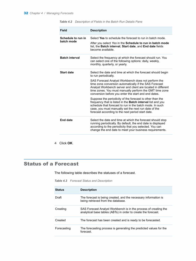
Table 4.2 Description of Fields in the Batch Run Details Pane
Field Description
Schedule to run in batch mode
Select Yes to schedule the forecast to run in batch mode.
After you select Yes in the Schedule to run in batch mode list, the Batch interval, Start date, and End date fields become available.
Batch interval Select the frequency at which the forecast should run. You can select one of the following options: daily, weekly, monthly, quarterly, or yearly.
Start date Select the date and time at which the forecast should begin to run periodically.
SAS Forecast Analyst Workbench does not perform the time zone conversion automatically if the SAS Forecast Analyst Workbench server and client are located in different time zones. You must manually perform the GMT time zone conversion before you enter the start and end dates.
Suppose the periodicity of the forecast is other than the frequency that is listed in the Batch interval list and you schedule that forecast to run in the batch mode. In such case, you must manually set the next run date of the forecast according to the next period start date.
End date Select the date and time at which the forecast should stop running periodically. By default, the end date is displayed according to the periodicity that you selected. You can change the end date to meet your business requirements.
4 Click OK.
Status of a Forecast
The following table describes the statuses of a forecast.
Table 4.3 Forecast Status and Description
Status Description
Draft The forecast is being created, and the necessary information is being retrieved from the database.
Creating SAS Forecast Analyst Workbench is in the process of creating the analytical base tables (ABTs) in order to create the forecast.
Created The forecast has been created and is ready to be forecasted.
Forecasting The forecasting process is generating the predicted values for the forecast.
32 Chapter 4 / Managing Forecasts

Status Description
Forecasted The predicted values of the forecast have been generated.
Error: In create An error occurred while the forecast was being created.
Error: In forecasting
An error occurred while the predicted values for the forecast were being generated.
Accepted The statistical model has been applied to the forecast, and the predicted values are satisfactory.
Scheduled The forecast is scheduled to run periodically in batch mode.
Ready to create The forecast has been copied. You can edit the forecast in order to create a new one.
Warning: Forecasted with errors
The predicted values of the forecast have been generated, but at least one time series is in error.
Deleting SAS Forecast Analyst Workbench is deleting the forecast and its relevant information, such as its metadata, analytical base tables, and so on.
Error: In delete An error occurred while the forecast was being deleted.
Accepting The forecast is being accepted.
Refreshing data SAS Forecast Analyst Workbench is refreshing the forecast.
Error: In update An error occurred while the forecast data was being updated.
Error: In accept An error occurred while the forecast was being accepted.
Obtaining NPF data
The data of a new product forecasting project data is being integrated with a forecast.
Error: In obtaining NPF data
An error occurred while the data of a new product forecasting project was being integrated with a forecast.
Obtaining modeling project data
SAS Forecast Analyst Workbench is obtaining data from the modeling project and is integrating that data with the linked forecast.
Error: In obtaining modeling project data
An error occurred while obtaining data from the modeling project.
Error: No valid data
An error occurred while a forecast was being created. The error occurred because SAS Forecast Analyst Workbench did not find the data required to create the forecast.
Status of a Forecast 33

34 Chapter 4 / Managing Forecasts

Part 3Generating Predicted Values
Chapter 5Workflow for Generating Predicted Values . . . . . . . . . . . . . . . . . . . . . . . . . . . 37
Chapter 6Generating and Analyzing Predicted Values . . . . . . . . . . . . . . . . . . . . . . . . . 41
Chapter 7Viewing Details of a Forecast . . . . . . . . . . . . . . . . . . . . . . . . . . . . . . . . . . . . . . 61
35

36
5
Workflow for Generating Predicted Values
Workflow for Generating Predicted Values . . . . . . . . . . . . . . . . . . . . . . . . . . . . . . . . . . 37
Status of a Forecast and Tasks Permitted in the Model Management View . . . 39
Workflow for Generating Predicted Values
Use the following workflow to choose the most suitable statistical model and to predict values:
1 Select the time series that are most important to you. The Model Management view displays the data for the selected time series.
For more information about selecting the time series, see “Select Time Series” on page 41.
2 Use various tabs of the Model Management view to view the time series and their actual and forecasted values. You can view the time series that are modified in the Administration workspace on the Changed Time Series tab.
For more information about the Hierarchy View tab and the Table View tab, see “View Information about Time Series” on page 62.
For more information about the Changed Time Series tab, see “View Information about Changed Time Series” on page 64.
3 Diagnose the forecast so that the best suitable statistical model is applied and predicted values are generated. The status of the forecast changes from Created to Forecasted.
For more information about diagnosing a forecast, see “Diagnose a Forecast” on page 43.
4 After the predicted values are obtained, consider the following factors when you examine them:
n the data that is available to you
n the purpose of your forecasting
n your organizational environment
n current market conditions
n the suite of products that you selected for generating the values
37
n the goals of your organization or department
n constraints
Compare the predicted values that are generated for the historical period with the actual values. You can use the prediction error, the root mean square error (RMSE), and the mean absolute percent error (MAPE) to compare the predicted values. You can also use graphs to compare the actual values with the predicted values.
For more information about RMSE and MAPE, see “View Model Information” on page 66.
5 If the prediction error, RMSE, and MAPE are not satisfactory, consider improving the forecast. You can perform one of the following tasks:
n edit parameters for the entire forecast, or for a single or multiple time series.
For more information about editing parameters, see “About Editing Parameters” on page 43.
n analyze the forecast in SAS Forecast Studio. You can generate different models, add events, and create scenarios in the SAS Forecast Studio, and then apply them.
For more information about modeling projects, see Chapter 8, “Introduction to Modeling Projects,” on page 71.
6 Rediagnose the forecast. When you rediagnose, SAS Forecast Analyst Workbench performs the following tasks:
1 considers the edited parameters to build models
2 selects the most suitable model
3 calculates the predicted values for the selected time series or for the entire forecast
4 reconciles the forecasted values
For more information about rediagnosing the forecast, see “Rediagnose a Forecast” on page 57.
7 Repeat steps 3 through 6 until the prediction error, RMSE, MAPE, and forecasted values are satisfactory.
8 Reconcile the forecast again to remove conflicts from the forecasted values if you have performed one of the following actions:
n analyzed the node or time series in SAS Forecast Studio and then promoted the forecast results and models in SAS Forecast Analyst Workbench
n edited or rediagnosed some of the time series
n changed and evaluated the default model of a time series
n rerun the forecast process for the selected time series
For more information about reconciling the forecast, see “Reconcile a Forecast” on page 57.
38 Chapter 5 / Workflow for Generating Predicted Values

9 Rerun the forecast to evaluate the predicted values of the selected time series whose parameters are changed. You can also perform this task on the entire forecast.
Fore more information about rerunning the forecast, see “Rerun the Forecast” on page 59.
10 After you are satisfied with the model that is applied to the forecast and the results, you can accept the forecast. The status of the forecast changes from Forecasted to Accepted.
For more information about accepting the forecast, see “Accept a Forecast” on page 59.
11 Refresh the forecast. When you refresh a forecast that is in the Created status, SAS Forecast Analyst Workbench refreshes actual values and includes newly added time series with their actual data. When you refresh a forecast that is in the Forecasted or Accepted status, SAS Forecast Analyst Workbench includes all latest time series, refreshes actual values, generates the predicted values, and changes the forecast status to Forecasted.
Status of a Forecast and Tasks Permitted in the Model Management View
You can open a forecast in the Model Management view. The following table lists the tasks that you can perform in the Model Management view, depending on the status of the forecast.
Table 5.1 Forecast Status and Permitted Tasks in the Model Management View
State of the forecast
Tasks that you can perform in the Model Management view
Information that you can view in the Model Management view
Created n edit parameters for the forecastn diagnose the forecastn set parameters for multiple time series
n actual values for the entire period, in tabular and graphical form
n time series in hierarchy or tabular form. When you are viewing the time series in tabular form, you can filter it.
Forecasted n edit parameters for the entire forecast or for the time series that you select
n evaluate a single time series, compare the two models, and set one of them as the default model
n analyze the entire forecast, a few nodes of the hierarchy, or the selected time series in SAS Forecast Studio
n reconcile the forecastn rerun the forecastn rediagnose the forecastn accept the forecastn perform scenario analysis
n actual values for the entire period, in tabular and graphical form
n predicted values for the entire periodn prediction error for the historical valuesn upper control limit and lower control limit
of the predicted valuesn model information such as name of the
model that is applied to the forecast, the type and source of the model, and the MAPE and RMSE of the model
n time series that are linked to the product succession on the Changed Time Series tab
Status of a Forecast and Tasks Permitted in the Model Management View 39

State of the forecast
Tasks that you can perform in the Model Management view
Information that you can view in the Model Management view
Accepted n edit parameters for the entire forecast or for the time series that you select
n evaluate a single time series, compare the two models, and set one of them as the default model
n analyze the entire forecast or the selected time series in SAS Forecast Studio
n reconcile the forecastn rediagnose the forecastn rerun the forecastn perform scenario analysis
n actual values for the entire period, in tabular and graphical form
n predicted values for the entire periodn prediction errorn upper control limit and lower control limit
of the predicted valuesn model information such as the name of
the model that is applied to the forecast, the type and source of the model, and the MAPE and RMSE of the model
40 Chapter 5 / Workflow for Generating Predicted Values

6
Generating and Analyzing Predicted Values
Select Time Series . . . . . . . . . . . . . . . . . . . . . . . . . . . . . . . . . . . . . . . . . . . . . . . . . . . . . . . . . . 41
Diagnose Forecasts . . . . . . . . . . . . . . . . . . . . . . . . . . . . . . . . . . . . . . . . . . . . . . . . . . . . . . . . 42Overview of Diagnosing Forecasts . . . . . . . . . . . . . . . . . . . . . . . . . . . . . . . . . . . . . . . . . 42Diagnose a Forecast . . . . . . . . . . . . . . . . . . . . . . . . . . . . . . . . . . . . . . . . . . . . . . . . . . . . . . 43
Edit Parameters . . . . . . . . . . . . . . . . . . . . . . . . . . . . . . . . . . . . . . . . . . . . . . . . . . . . . . . . . . . . 43About Editing Parameters . . . . . . . . . . . . . . . . . . . . . . . . . . . . . . . . . . . . . . . . . . . . . . . . . 43Edit Parameters for the Entire Forecast . . . . . . . . . . . . . . . . . . . . . . . . . . . . . . . . . . . . 44Edit Parameters for Multiple Time Series . . . . . . . . . . . . . . . . . . . . . . . . . . . . . . . . . . . 44Evaluate a Time Series . . . . . . . . . . . . . . . . . . . . . . . . . . . . . . . . . . . . . . . . . . . . . . . . . . . 45Editing Parameter Fields . . . . . . . . . . . . . . . . . . . . . . . . . . . . . . . . . . . . . . . . . . . . . . . . . . 45
Select a Default Model . . . . . . . . . . . . . . . . . . . . . . . . . . . . . . . . . . . . . . . . . . . . . . . . . . . . . . 55
Create a Modeling Project . . . . . . . . . . . . . . . . . . . . . . . . . . . . . . . . . . . . . . . . . . . . . . . . . . 55
Rediagnose a Forecast . . . . . . . . . . . . . . . . . . . . . . . . . . . . . . . . . . . . . . . . . . . . . . . . . . . . . 57
Reconcile a Forecast . . . . . . . . . . . . . . . . . . . . . . . . . . . . . . . . . . . . . . . . . . . . . . . . . . . . . . . 57About Reconciling a Forecast . . . . . . . . . . . . . . . . . . . . . . . . . . . . . . . . . . . . . . . . . . . . . 57Steps to Reconcile a Forecast . . . . . . . . . . . . . . . . . . . . . . . . . . . . . . . . . . . . . . . . . . . . . 58
Accept a Forecast . . . . . . . . . . . . . . . . . . . . . . . . . . . . . . . . . . . . . . . . . . . . . . . . . . . . . . . . . . 59
Rerun the Forecast . . . . . . . . . . . . . . . . . . . . . . . . . . . . . . . . . . . . . . . . . . . . . . . . . . . . . . . . . 59
Select Time Series
If the forecast contains too many time series, then you can choose the time series that are most important to you.
To select specific time series:
1 Double-click a forecast in the Forecasts category of the Forecast Plans workspace.
2 In the Model Management view, click . The Search Time Series wizard appears. The Search Time Series wizard displays the hierarchy levels that you selected in the forecast.
41
3 Select the hierarchy values for which you want to view the data in the Model Management view. Click Next to select the time series in each level.
You can view the number of time series that you have selected in the node at each step of the wizard.
4 Click Finish.
The Hierarchy View tab in the Model Management view displays the data for the time series that you selected. All actions that you take in the Model Management view are performed on all the time series that are included in the forecast.
5 (Optional) Reset the time series that you selected by clicking the button on the Forecast category of Forecast Plans workspace.
6 View information about the time series that you selected. This information is located on the Hierarchy View tab, the Table View tab, and the Changed Time Series tab in the Model Management view. For more information about how to interpret this information, see Chapter 7, “Viewing Details of a Forecast,” on page 61.
Diagnose Forecasts
Overview of Diagnosing Forecasts
Diagnose a forecast in order to find the most suitable statistical model and generate the predicted values for future periods. When you diagnose a forecast, the forecasting process analyzes the data and applies the appropriate model to the time series that are included in all hierarchy levels up to the forecast leaf level.
For all levels below the forecast leaf level, the values are predicted by using the disaggregation method. The predictions generated at the forecast leaf level are disaggregated to the time series included in the levels below the forecast leaf level. The disaggregation process is based on the proportion of the historical data that is included in a time series to the value at the forecast leaf level. For example, when the total value for the historical data at a time series A is 100 and the total value of the historical data at its parent time series is 200, the proportion is 0.5.The forecasting process uses SAS Forecast Server. The process is used for levels up to and including the forecast leaf level. The demand that is obtained through the disaggregation method is called dependent demand. SAS Forecast Analyst Workbench does not display the upper and lower confidence limits for the dependent demand time series.
After SAS Forecast Analyst Workbench diagnoses the forecast, it displays the following information:
n predicted demand values for the historical period and for the planning horizon (that is, for future period)
n prediction error for historical predicted values
n forecast upper confidence limit (UCL) for future predicted values
n forecast lower confidence limit (LCL) for future predicted values
42 Chapter 6 / Generating and Analyzing Predicted Values

n significant events that are applied in the model
n significant independent variables that are applied in the model
Diagnose a Forecast
The following prerequisites apply for diagnosing forecasts:
n You must have permission to diagnose the forecast. For more information, contact your system administrator.
n The forecast must be in the Created state.
To diagnose a forecast:
1 Do one of the following tasks:
n In the Forecast Plans workspace, select a forecast, and click .
n Perform the following steps:
1 In the Forecasts category of the Forecast Plans workspace, double-click a forecast.
The Model Management view appears.
2 Click Diagnose.
SAS Forecast Analyst Workbench starts generating the predicted values for the forecast and closes the Model Management view. The state of the forecast changes from Created to Forecasting. After the forecasting process is complete, the state of the forecast changes to Forecasted.
2 Click the Model Information tab to view the model-related information.
3 Click the Summary tab and the Plot view to view the predicted values.
Note: SAS Forecast Analyst Workbench does not calculate the predicted values for the time series that result in an error during forecasting. Therefore, even though the status of the forecast is Forecasted, some time series might not contain predicted values. You must select the individual time series in order to view their predicted values.
If you defined the succession settings, SAS Forecast Analyst Workbench uses the succession settings for these time series.
Edit Parameters
About Editing Parameters
You can edit parameters for the entire forecast, for multiple time series, or for a specific time series in order to improve the forecast. When you edit parameters for the time series, you can evaluate the predicted values and the model.
You can choose to apply the ARIMAX, ESM, or UCM model to the time series or to the forecast. You can also define the model selection and forecasting parameters, and specify the events settings. If you enable the selection of
Edit Parameters 43

multiple model types, SAS Forecast Analyst Workbench applies the best fit model. After you edit parameters for the entire forecast or for multiple time series, you must rediagnose the forecast. When you edit the parameters for a single time series, you can evaluate it.
Edit Parameters for the Entire Forecast
To edit the parameters for the entire forecast:
1 In the Model Management view, click , and then select Edit parameters for forecast. The Parameter Settings window appears.
2 Edit the parameters, and then click OK.
Note: When you are editing parameters for the entire forecast, the Events tab of the Parameter Settings window is not available.
For more information about editing the parameters, see “Editing Parameter Fields” on page 45.
3 Click Diagnose to diagnose the forecast in order to apply the parameters and calculate the new predicted values when the forecast is in the Created state.
Click Rediagnose to rediagnose the forecast when the forecast is in the Forecasted or Accepted state.
For more information about diagnosing a forecast, see “Diagnose a Forecast” on page 43. For more information about rediagnosing the forecast, see “Rediagnose a Forecast” on page 57.
Edit Parameters for Multiple Time Series
You can select multiple time series and edit their parameters. The selected time series must contain sufficient historical data.
You cannot edit the parameters of a time series that you selected on the Changed Time Series tab of the Model Management view.
To edit parameters for multiple time series:
1 In the Model Management view, press and hold the Ctrl key and select multiple time series.
2 Click , and then select Edit parameters for time series. The Parameter Settings window appears.
3 Edit the parameters, and then click OK.
Note: The mark next to a field indicates that the value that is currently displayed for that time series is different from the actual value. This mark appears when you select multiple time series that have different values.
4 Click Rediagnose to recalculate the predicted values when you have edited parameters for the selected time series.
For more information about rediagnosing the forecast, see “Rediagnose a Forecast” on page 57
44 Chapter 6 / Generating and Analyzing Predicted Values

Evaluate a Time Series
You can evaluate a time series and check the forecasted values for that time series.
To evaluate a time series:
1 In the Model Management view, select a forecast-level time series.
2 Click , and then select Edit parameters for time series. The Edit Parameters window appears.
3 Edit the parameters, and then click Evaluate.
SAS Forecast Analyst Workbench uses the edited parameters to build models and to predict the future values by using the most suitable model. For more information about editing parameters fields, see “Editing Parameter Fields” on page 45.
4 Click the Model Information tab to display the model that was applied before the parameters were edited and another model with the new parameters.
You can compare the values of the default model with the values of the evaluated model. You must select one model to be the default model before continuing your work. For more information about selecting a default model, see “Select a Default Model” on page 55.
Editing Parameter Fields
Define ARIMAX Model Parameters
You can define the autoregressive integrated moving average with exogenous inputs (ARIMAX) model parameters.
Click the Model Generation tab and select the Use ARIMAX option. Specify the following fields.
Table 6.1 Field Descriptions for the Use ARIMAX Option
Field Description
Use default ARIMAX
Select Yes to use the default ARIMAX model parameters.
Apply default ARIMAX parameters of SAS Forecast Studio
Select this check box to apply the ARIMAX model that is identical in SAS Forecast Studio and apply its parameters.
Note: After you select this check box, only the Identification order when inputs and events are specified field is available.
Nonseasonal Options
Edit Parameters 45

Field Description
AR orders (p) Select a range for the nonseasonal autoregressive (AR) orders. The valid range for nonseasonal AR orders is 0–13. The default value for the minimum AR order is 0, and the default value for the maximum AR order is 5.
MA orders (q) Select a range for the nonseasonal moving average (MA) orders. The valid range for nonseasonal MA orders is 0–13. The default value for the minimum MA order is 0, and the default value for the maximum MA order is 5.
Seasonal Options
AR Orders (P) Select a range for the seasonal AR orders. The valid range for nonseasonal AR orders is 0–2. The default value for the minimum AR order is 0, and the default value for the maximum AR order is 2.
MA orders (Q) Select a range for the seasonal MA orders. The valid range for nonseasonal MA orders is 0–2. The default value for the minimum MA order is 0, and the default value for the maximum AR order is 2.
Numerator Select a range for the numerator orders of the transfer function of the ARIMAX model. The valid range for the numerator orders is 0–2. The default value for the minimum numerator is 0, and the default value for the maximum numerator is 2.
Denominator Select a range for the denominator orders of the transfer function of the ARIMAX model from the list. The valid range for the denominator orders is 0–2. The default value for the minimum denominator is 0, and the default value for the maximum denominator is 2.
Criterion Select the criterion for the tentative ARMA order selection. The list contains the following options:n SBC: Schwarz Bayesian information criterion
Note: This is the default criterion.n AIC: Akaike information criterion
Significance level to decide AR and MA orders
Enter the significance level to use as a cutoff value for determining the AR and MA orders. The significance level must be in the range (0, 1).
Method for choosing tentative ARMA order
Select the method for choosing the tentative ARMA order. The list contains the following options:n CLS: conditional least squares method. This is the default
method.n ULS: unconditional least squares methodn ML: maximum likelihood method
46 Chapter 6 / Generating and Analyzing Predicted Values
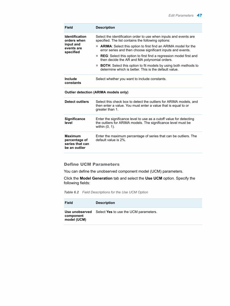
Field Description
Identification orders when input and events are specified
Select the identification order to use when inputs and events are specified. The list contains the following options:n ARIMA: Select this option to first find an ARIMA model for the
error series and then choose significant inputs and events.n REG: Select this option to first find a regression model first and
then decide the AR and MA polynomial orders.n BOTH: Select this option to fit models by using both methods to
determine which is better. This is the default value.
Include constants
Select whether you want to include constants.
Outlier detection (ARIMA models only)
Detect outliers Select this check box to detect the outliers for ARIMA models, and then enter a value. You must enter a value that is equal to or greater than 1.
Significance level
Enter the significance level to use as a cutoff value for detecting the outliers for ARIMA models. The significance level must be within (0, 1).
Maximum percentage of series that can be an outlier
Enter the maximum percentage of series that can be outliers. The default value is 2%.
Define UCM Parameters
You can define the unobserved component model (UCM) parameters.
Click the Model Generation tab and select the Use UCM option. Specify the following fields:
Table 6.2 Field Descriptions for the Use UCM Option
Field Description
Use unobserved component model (UCM)
Select Yes to use the UCM parameters.
Edit Parameters 47

Field Description
Components to be included in UCM
Select a component to test for inclusion in the UCM. The list contains the following options:n all: test which components, variances, or both are significant in
the model. This is the default option. When the series contains seasonality information, the Irregular, Level, Slope, and Season components are included. Otherwise, the Irregular, Level, Slope, and Cycle components are included.
n Autoreg: test whether an autoregressive component is significant in the model.
n Cycle: test whether two Cycle components are significant in the model. The two Cycle components are included and the Level component is added. When the series contains seasonality information, the Cycle component is not tested.
n Deplag: test whether a dependent lag component is significant in the model. Only the order 1 is included.
n Irregular: test whether an irregular component is significant in the model.
n Level: test whether a level component is significant in the model.
n Season: test whether a season component is significant in the model. When the series contains seasonality information, the Season component is not tested.
n Slope: test whether a slope component is significant in the model.
Significance level for model components
Enter the significance level to use as a cutoff value for deciding which components or variances are significant. The significance level must be within (0, 1)
Define ESM Parameters
You can define the exponential smoothing model (ESM) parameters.
Click the Model Generation tab and select the Use ESM option. Specify the following fields:
Table 6.3 Field Descriptions for the Use ESM Option
Field Description
Use exponential smoothing model (ESM)
Select Yes to use the ESM parameters.
48 Chapter 6 / Generating and Analyzing Predicted Values

Field Description
ESM method Select the ESM method from the list.n Best: Select this option to fit the best candidate smoothing model
(SIMPLE, DOUBLE, LINEAR, DAMPTREND, SEASONAL, WINTERS, ADDWINTERS). This is the default option.
n Best nonseasonal: Select this option to fit the best candidate nonseasonal smoothing model (SIMPLE, DOUBLE, LINEAR, DAMPTREND).
n Best seasonal: Select this option to fit the best candidate seasonal smoothing model (SEASONAL, WINTERS, ADDWINTERS).
Define Other Parameters
You can define the other parameters for a time series.
Click the Model Generation tab and select the Other Options option. Specify the following fields:
Table 6.4 Field Descriptions for the Other Options Option
Field Description
Trend Diff Specify the simple differencing for the dependent series. The list contains the following options:n Auto: Select this option to test for simple differencing. This is the
default option.n Nonnegative number: Select this option to specify the simple
differencing order. n None: Select this option to specify that simple differencing is not
used.
Trend SDiff Select an option from list to specify the seasonal differencing for the dependent series.n Auto: Select this option to test for seasonal differencing. This is
the default option.n Nonnegative number: Select this option to specify the seasonal
differencing order.n None: Select this option to specify that seasonal differencing is not
used.
Diagnose independent variables separately
Select this check box, and then select an option from the list to diagnose the independent variables of the forecast separately.n Both: Select this option to specify that the log transform and trend
testing of the input variables are applied independently of the variable to be forecast. This is the default option.
n Transform: Select this option to specify that the log transform testing of the input variables is applied independently of the variable to be forecast.
n Trend: Select this option to specify that the trend testing of the input variables is applied independently of the variable to be forecast.
Edit Parameters 49
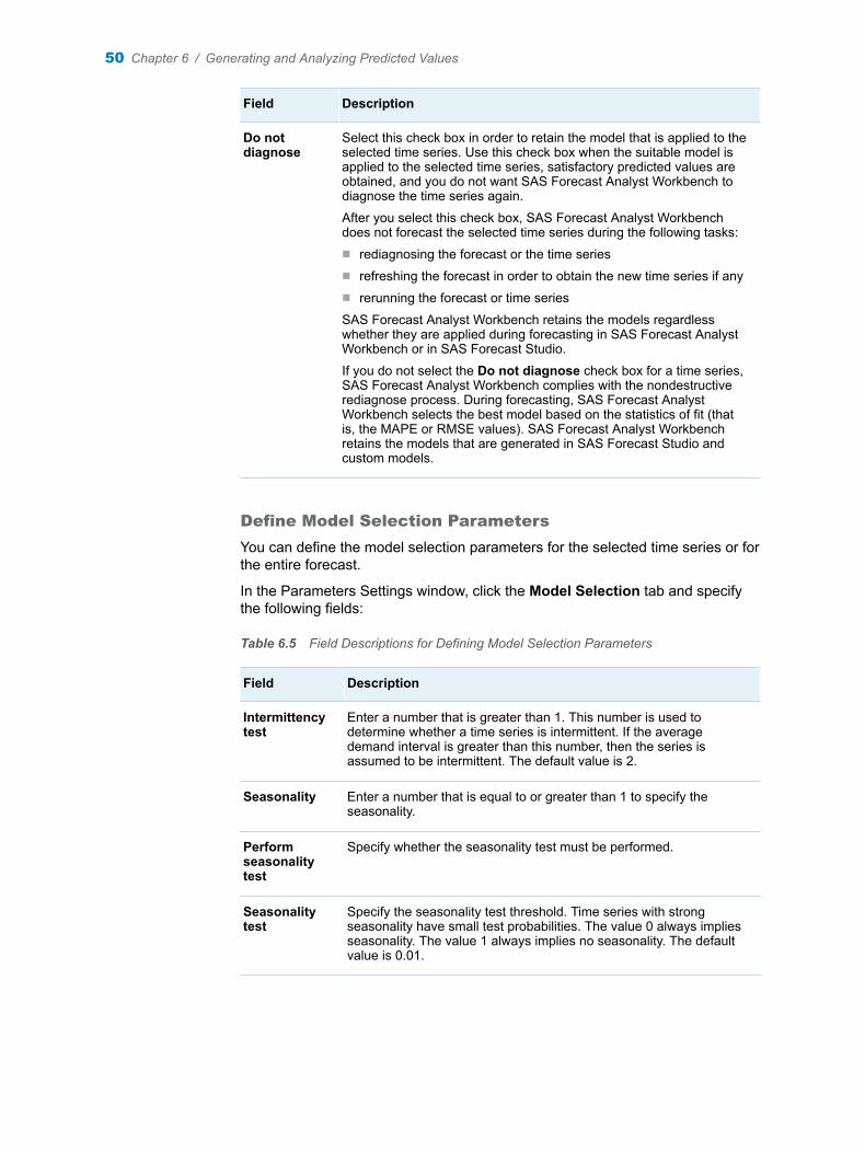
Field Description
Do not diagnose
Select this check box in order to retain the model that is applied to the selected time series. Use this check box when the suitable model is applied to the selected time series, satisfactory predicted values are obtained, and you do not want SAS Forecast Analyst Workbench to diagnose the time series again.
After you select this check box, SAS Forecast Analyst Workbench does not forecast the selected time series during the following tasks:n rediagnosing the forecast or the time seriesn refreshing the forecast in order to obtain the new time series if anyn rerunning the forecast or time series
SAS Forecast Analyst Workbench retains the models regardless whether they are applied during forecasting in SAS Forecast Analyst Workbench or in SAS Forecast Studio.
If you do not select the Do not diagnose check box for a time series, SAS Forecast Analyst Workbench complies with the nondestructive rediagnose process. During forecasting, SAS Forecast Analyst Workbench selects the best model based on the statistics of fit (that is, the MAPE or RMSE values). SAS Forecast Analyst Workbench retains the models that are generated in SAS Forecast Studio and custom models.
Define Model Selection Parameters
You can define the model selection parameters for the selected time series or for the entire forecast.
In the Parameters Settings window, click the Model Selection tab and specify the following fields:
Table 6.5 Field Descriptions for Defining Model Selection Parameters
Field Description
Intermittency test
Enter a number that is greater than 1. This number is used to determine whether a time series is intermittent. If the average demand interval is greater than this number, then the series is assumed to be intermittent. The default value is 2.
Seasonality Enter a number that is equal to or greater than 1 to specify the seasonality.
Perform seasonality test
Specify whether the seasonality test must be performed.
Seasonality test
Specify the seasonality test threshold. Time series with strong seasonality have small test probabilities. The value 0 always implies seasonality. The value 1 always implies no seasonality. The default value is 0.01.
50 Chapter 6 / Generating and Analyzing Predicted Values
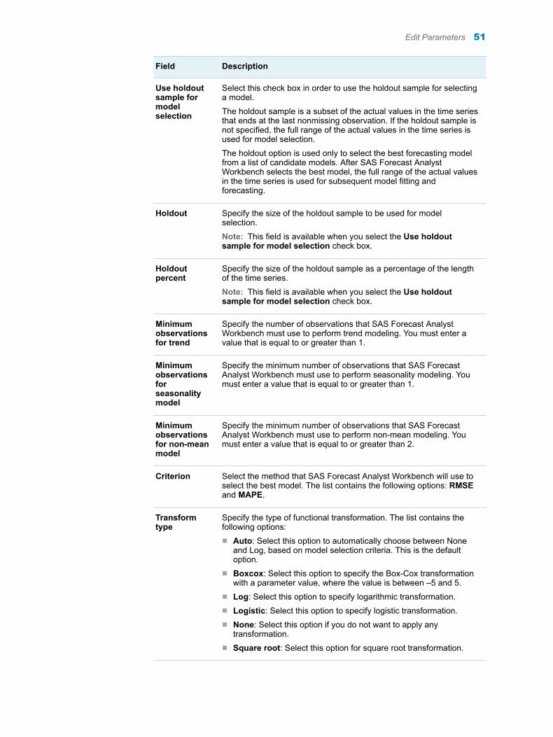
Field Description
Use holdout sample for model selection
Select this check box in order to use the holdout sample for selecting a model.
The holdout sample is a subset of the actual values in the time series that ends at the last nonmissing observation. If the holdout sample is not specified, the full range of the actual values in the time series is used for model selection.
The holdout option is used only to select the best forecasting model from a list of candidate models. After SAS Forecast Analyst Workbench selects the best model, the full range of the actual values in the time series is used for subsequent model fitting and forecasting.
Holdout Specify the size of the holdout sample to be used for model selection.
Note: This field is available when you select the Use holdout sample for model selection check box.
Holdout percent
Specify the size of the holdout sample as a percentage of the length of the time series.
Note: This field is available when you select the Use holdout sample for model selection check box.
Minimum observations for trend
Specify the number of observations that SAS Forecast Analyst Workbench must use to perform trend modeling. You must enter a value that is equal to or greater than 1.
Minimum observations for seasonality model
Specify the minimum number of observations that SAS Forecast Analyst Workbench must use to perform seasonality modeling. You must enter a value that is equal to or greater than 1.
Minimum observations for non-mean model
Specify the minimum number of observations that SAS Forecast Analyst Workbench must use to perform non-mean modeling. You must enter a value that is equal to or greater than 2.
Criterion Select the method that SAS Forecast Analyst Workbench will use to select the best model. The list contains the following options: RMSE and MAPE.
Transform type
Specify the type of functional transformation. The list contains the following options:n Auto: Select this option to automatically choose between None
and Log, based on model selection criteria. This is the default option.
n Boxcox: Select this option to specify the Box-Cox transformation with a parameter value, where the value is between –5 and 5.
n Log: Select this option to specify logarithmic transformation.n Logistic: Select this option to specify logistic transformation.n None: Select this option if you do not want to apply any
transformation. n Square root: Select this option for square root transformation.
Edit Parameters 51
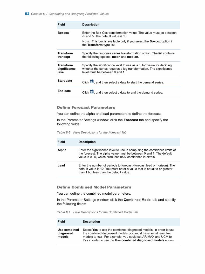
Field Description
Boxcox Enter the Box-Cox transformation value. The value must be between -5 and 5. The default value is 1.
Note: This box is available only if you select the Boxcox option in the Transform type list.
Transform transopt
Specify the response series transformation option. The list contains the following options: mean and median.
Transform significance level
Specify the significance level to use as a cutoff value for deciding whether the series requires a log transformation. The significance level must be between 0 and 1.
Start date Click , and then select a date to start the demand series.
End date Click , and then select a date to end the demand series.
Define Forecast Parameters
You can define the alpha and lead parameters to define the forecast.
In the Parameter Settings window, click the Forecast tab and specify the following fields:
Table 6.6 Field Descriptions for the Forecast Tab
Field Description
Alpha Enter the significance level to use in computing the confidence limits of the forecast. The alpha value must be between 0 and 1. The default value is 0.05, which produces 95% confidence intervals.
Lead Enter the number of periods to forecast (forecast lead or horizon). The default value is 12. You must enter a value that is equal to or greater than 1 but less than the default value.
Define Combined Model Parameters
You can define the combined model parameters.
In the Parameter Settings window, click the Combined Model tab and specify the following fields:
Table 6.7 Field Descriptions for the Combined Model Tab
Field Description
Use combined diagnosed models
Select Yes to use the combined diagnosed models. In order to use the combined diagnosed models, you must have set at least two models to Yes. For example, you could set ARIMAX and UCM to Yes in order to use the Use combined diagnosed models option.
52 Chapter 6 / Generating and Analyzing Predicted Values
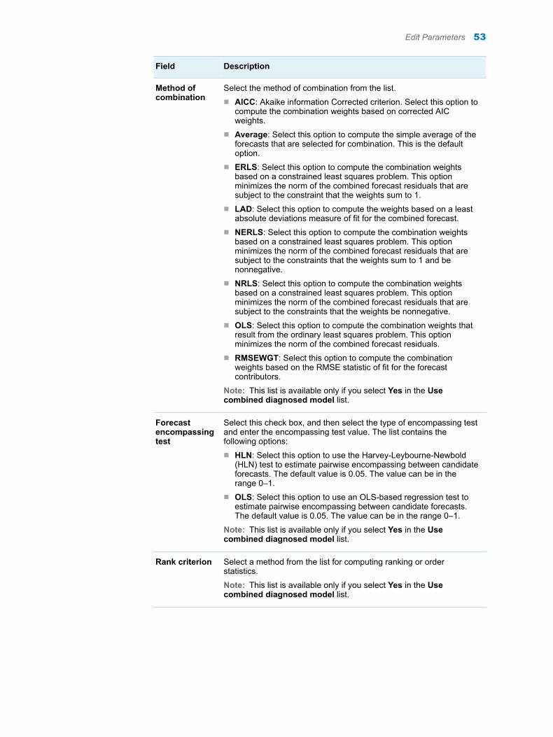
Field Description
Method of combination
Select the method of combination from the list.n AICC: Akaike information Corrected criterion. Select this option to
compute the combination weights based on corrected AIC weights.
n Average: Select this option to compute the simple average of the forecasts that are selected for combination. This is the default option.
n ERLS: Select this option to compute the combination weights based on a constrained least squares problem. This option minimizes the norm of the combined forecast residuals that are subject to the constraint that the weights sum to 1.
n LAD: Select this option to compute the weights based on a least absolute deviations measure of fit for the combined forecast.
n NERLS: Select this option to compute the combination weights based on a constrained least squares problem. This option minimizes the norm of the combined forecast residuals that are subject to the constraints that the weights sum to 1 and be nonnegative.
n NRLS: Select this option to compute the combination weights based on a constrained least squares problem. This option minimizes the norm of the combined forecast residuals that are subject to the constraints that the weights be nonnegative.
n OLS: Select this option to compute the combination weights that result from the ordinary least squares problem. This option minimizes the norm of the combined forecast residuals.
n RMSEWGT: Select this option to compute the combination weights based on the RMSE statistic of fit for the forecast contributors.
Note: This list is available only if you select Yes in the Use combined diagnosed model list.
Forecast encompassing test
Select this check box, and then select the type of encompassing test and enter the encompassing test value. The list contains the following options:n HLN: Select this option to use the Harvey-Leybourne-Newbold
(HLN) test to estimate pairwise encompassing between candidate forecasts. The default value is 0.05. The value can be in the range 0–1.
n OLS: Select this option to use an OLS-based regression test to estimate pairwise encompassing between candidate forecasts. The default value is 0.05. The value can be in the range 0–1.
Note: This list is available only if you select Yes in the Use combined diagnosed model list.
Rank criterion Select a method from the list for computing ranking or order statistics.
Note: This list is available only if you select Yes in the Use combined diagnosed model list.
Edit Parameters 53
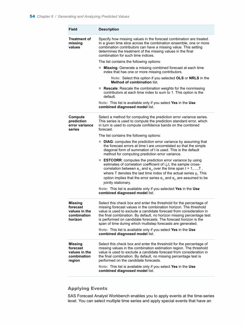
Field Description
Treatment of missing values
Specify how missing values in the forecast combination are treated. In a given time slice across the combination ensemble, one or more combination contributors can have a missing value. This setting determines the treatment of the missing values in the final combination for such time indices.
The list contains the following options:n Missing: Generate a missing combined forecast at each time
index that has one or more missing contributors.
Note: Select this option if you selected OLS or NRLS in the Method of combination list.
n Rescale: Rescale the combination weights for the nonmissing contributors at each time index to sum to 1. This option is the default.
Note: This list is available only if you select Yes in the Use combined diagnosed model list.
Compute prediction error variance series
Select a method for computing the prediction error variance series. This series is used to compute the prediction standard error, which in turn is used to compute confidence bands on the combined forecast.
The list contains the following options:n DIAG: computes the prediction error variance by assuming that
the forecast errors at time t are uncorrelated so that the simple diagonal form of summation of t is used. This is the default method for computing prediction error variance.
n ESTCORR: computes the prediction error variance by using estimates of correlation coefficient of i,j,t, the sample cross-correlation between ei,t and ej,t over the time span t = 1,....,T , where T denotes the last time index of the actual series yt. This option implies that the error series ei,t and ej,t are assumed to be jointly stationary.
Note: This list is available only if you selected Yes in the Use combined diagnosed model list.
Missing forecast values in the combination horizon
Select this check box and enter the threshold for the percentage of missing forecast values in the combination horizon. The threshold value is used to exclude a candidate forecast from consideration in the final combination. By default, no horizon missing percentage test is performed on candidate forecasts. The forecast horizon is the span of time during which multistep forecasts are generated.
Note: This list is available only if you select Yes in the Use combined diagnosed model list.
Missing forecast values in the combination region
Select this check box and enter the threshold for the percentage of missing values in the combination estimation region. The threshold value is used to exclude a candidate forecast from consideration in the final combination. By default, no missing percentage test is performed on the candidate forecasts.
Note: This list is available only if you select Yes in the Use combined diagnosed model list.
Applying Events
SAS Forecast Analyst Workbench enables you to apply events at the time-series level. You can select multiple time series and apply special events that have an
54 Chapter 6 / Generating and Analyzing Predicted Values

impact on the demand. You can select the events from a list of events that are available, or you can import events from the .csv file. You cannot clear the events that you selected while you were creating the forecast. Those events are applied across the forecast and thus you cannot clear them at the time-series level. You must edit the forecast to remove the events that are available at the entire forecast level.
Defining events at the time series level helps you apply the events that are specific to that time series.
For example, in a global car manufacturing organization, a particular model of a car is sold in Europe but not in Asia. You can define the Europe-specific events on that time series instead of defining Europe-specific events at the forecast level.
For more information about events and the guidelines, see “Events” on page 21.
Note: The Events tab in the Parameter Settings window is available when you are editing the parameters of the time series. This tab is not available when you are editing the parameters for the entire forecast.
Select a Default Model
When you edit the parameters of a time series, the Model Information tab displays two models. You can view the details of each model and select the most suitable model as the default model. After you select a default model, you must rediagnose the forecast.
The following prerequisites apply:
n The Model Information tab must contain multiple models.
n You must have permission to select a default model. For more information, contact your system administrator.
To select a default model:
1 On the Model Information tab of the Model Management view, select the most suitable model.
2 Click Set this model as forecast model.
The selected model is applied to the time series. Now, you must reconcile the forecast. For more information about reconciling the forecast, see “Reconcile a Forecast” on page 57.
Create a Modeling Project
You can create the modeling project to use the forecasting capabilities of SAS Forecast Studio and improve your forecast. You can create a modeling project in order to analyze the following items in SAS Forecast Studio:
n an entire forecast
n a selected hierarchy node
Create a Modeling Project 55

n an individual forecast-leaf-level time series
You cannot create a modeling project on a time series that is selected on the Changed Time Series tab of the Model Management view.
The following prerequisites apply:
n You must have permission to create the modeling project. For more information, contact your system administrator.
n The forecast must be in the Forecasted or Accepted state.
To create a modeling project:
1 Double-click a forecast in the Forecasts category of the Forecast Plans workspace.
The Model Management view appears.
2 (Optional) Click the Hierarchy View tab, and select one or more hierarchy nodes or time series.
3 Click . The Analyze in SAS Forecast Studio window appears.
4 Select one of the following options:
n Select Analyze all time series of the forecast to analyze the entire forecast in SAS Forecast Studio.
SAS Forecast Analyst Workbench considers all nodes up to and including the forecast leaf level. All nodes below the forecast leaf level are not considered when you create a modeling project.
n Select Analyze on the selected hierarchy node to base the analysis on the selected hierarchy node.
SAS Forecast Analyst Workbench creates the modeling project with the selected hierarchy node and all nodes that are below the selected hierarchy node up to and including the forecast leaf level.
n Select Analyze on individual time series to base the analysis on the individual forecast-leaf-level time series of the forecast.
5 Enter the name for the modeling project.
Note: This is a required field.
The project name must be a valid SAS name. For more information about SAS naming conventions, see SAS Language Reference: Concepts.
6 Enter a description of the project.
7 Click OK.
The Modeling category displays the project that you created. By default, the project is created in the Submitted state.
For more information about modeling projects, see Chapter 8, “Introduction to Modeling Projects,” on page 71.
56 Chapter 6 / Generating and Analyzing Predicted Values

Rediagnose a Forecast
You can rediagnose the forecast in order to reevaluate the forecast models and recalculate the predicted values. You can rediagnose the forecast for various reasons. For example, you might want to generate new forecasted values after you edit the parameters for the entire forecast or for some time series. When you rediagnose the forecast, the forecast process considers modified factors such as the parameters that you edited, and so on.
The following prerequisites apply:
n You must have permission to rediagnose the forecast. For more information, contact your system administrator.
n The forecast must be in one of the following states: Forecasted, Accepted, or Error: In forecasting.
To rediagnose a forecast, do one of the following:
n In the Forecast Plans workspace, select a forecast, and click .
n Perform the following steps:
1 In the Forecasts category of the Forecast Plans workspace, double-click a forecast.
The Model Management view appears.
2 Click Rediagnose.
SAS Forecast Analyst Workbench starts rediagnosing the forecast. The Model Management view closes and the forecast status changes to Forecasting.
SAS Forecast Analyst Workbench uses the information that you modified to diagnose the most suitable model, and it uses the model to forecast the future values. SAS Forecast Analyst Workbench retains the forecast models for the time series for which the Do not diagnose option is selected and uses those models to generate the forecasted values.
After the predicted values are generated for the forecast, its status changes to Forecasted. If an error occurs during forecasting, the forecast status changes to Error in forecasting.
Reconcile a Forecast
About Reconciling a Forecast
You must reconcile the forecast to remove any conflicts if you have performed one of the following tasks:
n analyzed the node or time series in SAS Forecast Studio and then promoted the results to SAS Forecast Analyst Workbench
n edited the parameter settings for some of the time series
n evaluated a time series and changed its default model
Reconcile a Forecast 57

n reran a time series
SAS Forecast Analyst Workbench uses one of the following reconciliation methods, which you defined when you created the forecast:
top-downaggregates the data from the lowest levels in the forecast and then uses these values to generate the forecasts at the highest level. SAS Forecast Analyst Workbench then uses this forecast and the reconciliation weights that are based on the forecast values at the lower levels to reconcile and adjust the forecasted values for lower levels in the hierarchy.
The top-down method enables you to remove excessive noise from the data at the lower levels of the hierarchy. However, you also might lose the pattern (such as the seasonality) in the forecast.
bottom-upuses the data at the lowest level of the hierarchy to generate the forecasts. These forecasts are then used to reconcile the forecasts for the higher levels in the hierarchy.
The bottom-up method enables you to see any patterns (such as seasonality) in the data. However, because you are at the lowest level of the hierarchy, you can also have too much noise or randomness in the data. Also, these forecasts might fail because the data at the lowest level of the hierarchy is sporadic or too sparse.
middle-outaggregates the data from the lower levels and then uses these values to generate the forecasts for the middle level. SAS Forecast Analyst Workbench uses the forecasts at the middle level to reconcile the forecasts for both the higher and lower levels. Some hierarchies have more than one middle level, so you need to specify the level that you want to use.
For more information about reconciliation, see SAS Forecast Server Procedures: User’s Guide.
Steps to Reconcile a Forecast
The following prerequisites apply:
n You must have permission to reconcile the forecast. For more information, contact your system administrator.
n The forecast must be in one of the following states: Forecasted, Accepted, or Error: In forecasting.
n The forecast must contain multiple hierarchy levels.
To reconcile a forecast:
1 Double-click a forecast in the Forecasts category of the Forecast Plans workspace.
The Model Management view appears.
2 Click Reconcile.
SAS Forecast Analyst Workbench starts reconciling the forecast and closes the Model Management view.
58 Chapter 6 / Generating and Analyzing Predicted Values

Accept a Forecast
You can accept a forecast when you are satisfied with the RMSE, MAPE, and predicted values. When you accept a forecast, its status changes from Forecasted to Accepted.
After you accept a forecast, you can perform tasks on it. For more information about tasks that you can perform on a forecast that is in the Accepted state, see Table 5.1 on page 39. After you perform any of these tasks, the state of the forecast changes from Accepted to Forecasted. You must review the forecast values and accept the forecast again in order to change its status to Accepted.
The following prerequisites apply:
n You must have permission to accept the forecast. For more information, contact your system administrator.
n The forecast must be in the Forecasted or Warning: Forecasted with errors state.
To accept a forecast:
1 Double-click a forecast in the Forecasts category of the Forecast Plans workspace.
The Model Management view appears.
2 Click Accept.
The Model Management view closes and the state of the forecast changes to Accepted. After you accept the forecast, you can run it in batch mode so that SAS Forecast Analyst Workbench calculates the predicted values for the newly added time series and recalculates the predicted values for the existing time series based on the additional historical data.
When you accept a forecast that contains a scenario analysis performed on any of the time series, the predicted values of those time series are updated with the scenario values.
Rerun the Forecast
When you rerun the forecast, SAS Forecast Analyst Workbench recalculates the demand values. You can perform this task on the entire forecast or on the selected forecast-leaf-level time series.
The following prerequisites apply:
n You must have permission to rerun the forecast. For more information, contact your system administrator.
n The forecast must be in the Forecasted or Accepted state.
To rerun the forecast:
1 Double-click a forecast in the Forecasts category of the Forecast Plans workspace.
Rerun the Forecast 59
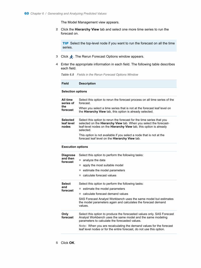
The Model Management view appears.
2 Click the Hierarchy View tab and select one more time series to run the forecast on.
TIP Select the top-level node if you want to run the forecast on all the time series.
3 Click . The Rerun Forecast Options window appears.
4 Enter the appropriate information in each field. The following table describes each field.
Table 6.8 Fields in the Rerun Forecast Options Window
Field Description
Selection options
All time series of the forecast
Select this option to rerun the forecast process on all time series of the forecast.
When you select a time series that is not at the forecast leaf level on the Hierarchy View tab, this option is already selected.
Selected leaf level nodes
Select this option to rerun the forecast for the time series that you selected on the Hierarchy View tab. When you select the forecast-leaf-level nodes on the Hierarchy View tab, this option is already selected.
This option is not available if you select a node that is not at the forecast leaf level on the Hierarchy View tab.
Execution options
Diagnose and then forecast
Select this option to perform the following tasks:n analyze the datan apply the most suitable modeln estimate the model parametersn calculate forecast values
Select and forecast
Select this option to perform the following tasks:n estimate the model parametersn calculate forecast demand values
SAS Forecast Analyst Workbench uses the same model but estimates the model parameters again and calculates the forecast demand values.
Only forecast
Select this option to produce the forecasted values only. SAS Forecast Analyst Workbench uses the same model and the same modeling parameters to calculate the forecasted values.
Note: When you are recalculating the demand values for the forecast leaf level nodes or for the entire forecast, do not use this option.
5 Click OK.
60 Chapter 6 / Generating and Analyzing Predicted Values

7
Viewing Details of a Forecast
Perform Frequent Tasks Related to Model Management . . . . . . . . . . . . . . . . . . . . . 61
View Information about Time Series . . . . . . . . . . . . . . . . . . . . . . . . . . . . . . . . . . . . . . . . . 62
Filter the Time Series . . . . . . . . . . . . . . . . . . . . . . . . . . . . . . . . . . . . . . . . . . . . . . . . . . . . . . . 63
View Information about Changed Time Series . . . . . . . . . . . . . . . . . . . . . . . . . . . . . . . 64
View Forecast Plots . . . . . . . . . . . . . . . . . . . . . . . . . . . . . . . . . . . . . . . . . . . . . . . . . . . . . . . . . 64
View Predicted Values and Summary Information for a Forecast . . . . . . . . . . . . 65
View Model Information . . . . . . . . . . . . . . . . . . . . . . . . . . . . . . . . . . . . . . . . . . . . . . . . . . . . . 66
View Information About Child Products . . . . . . . . . . . . . . . . . . . . . . . . . . . . . . . . . . . . . 67
View Future Values of Changed Time Series . . . . . . . . . . . . . . . . . . . . . . . . . . . . . . . . 67
Perform Frequent Tasks Related to Model Management
You can perform the following model management tasks in the Model Management view.
Table 7.1 Frequent Model Management Tasks
Task Button Description
Edit parameters
Click this button and then select the appropriate option:n Edit parameters for forecast: Select this option to edit
the parameters for the entire forecast.
For more information about editing parameters of the entire forecast, see “Edit Parameters for the Entire Forecast” on page 44
n Edit parameters for time series: Select this option to edit the parameters for the selected time series. SAS Forecast Analyst Workbench uses the parameters that you defined to apply the model and predict the values.
For more information about editing parameters of multiple forecast-leaf-level time series, see “Edit Parameters for Multiple Time Series” on page 44.
61

Task Button Description
Create a modeling project
Click this button to create a modeling project for the entire forecast, for the selected hierarchy node, or for the selected forecast-leaf-level time series. You can perform more analysis in SAS Forecast Studio, apply models, and promote the forecast.
For more information about analyzing the forecast or a time series in SAS Forecast Studio, see “Create a Modeling Project” on page 55.
Rerun the forecast
Click this button to rerun the entire forecast or to rerun the forecast for the selected forecast-leaf-level time series. Rerunning the forecast applies newly assigned parameters to the time series. Forecasts might change to acceptable levels.
For more information about running the forecast, see “Rerun the Forecast” on page 59.
Apply time series filter
Click this button to select the time series that are most important to you. The selected time series are displayed on the Hierarchy View tab in the Model Management view.
Reset filter Click this button to reset the time series filter. This button is available when you have applied the times series filter.
View Information about Time Series
You can view the following information about time series in the Model Management view:
n To display the time series in a tree view, click the Hierarchy View tab. Only time series that contain data are displayed. (You defined the time series when you created the forecast.) The forecasting process applies the statistical models up to the forecast leaf level, and then generates the predicted values. All levels below the forecast leaf level are forecasted with the disaggregation method.
o Expand or collapse the nodes to view the time series hierarchy. The icon denotes the forecast leaf level and the icon denotes the combined products.
o Select a time series and complete tasks such as edit parameters, create a modeling project, and so on. For more information, see Chapter 6, “Generating and Analyzing Predicted Values,” on page 41.
n To view the information about the time series in tabular form, select a time series on the Hierarchy View tab, and then click Refresh on the Table View tab. Only time series that contain data are displayed. You can select a time series and work on it in the Model Management view. You cannot edit parameters of a time series or analyze a time series in SAS Forecast Studio from the Table View. In order to perform edit parameters or analyze a time series in SAS Forecast Studio, select that time series in the Hierarchy View.
62 Chapter 7 / Viewing Details of a Forecast

The following information is displayed on the Table View tab.
Table 7.2 Information on the Table View Tab
Column Name Description
Parent Path
The path that starts from the parent and ends with the selected hierarchy value.
Name The name of the hierarchical value.
BOM Whether the bill of material is applicable for the selected time series. The column contains one of the following values:n Yes if you selected bill of material settings when you created the
forecast.n No if you did not select the bill of material settings when you
created the forecast.n NA if the bill of material settings are not applicable for the
product.
Note: This column displays a value only when you select a product at the forecast leaf level.
Forecast Status
One of the following forecast states for the hierarchical value: Normal, Failed to forecast, Forecasted with warnings, Disaggregated, and NPF-Forecasted.
MAPE The mean absolute percentage error.
RMSE The root mean square error.
Prediction APE
The prediction absolute percent error for the selected time series if the forecast has run at least twice in batch mode.
Prediction MAPE
The prediction mean absolute percent error for the selected time series if the forecast has run at least twice in batch mode.
Filter the Time Series
On the Table View tab, you can filter the time series based on the following parameters:
n Forecast Quality
n Forecast Status
n Seasonality
n Intermittency
n Trend
n Events
n Independent variables
Filter the Time Series 63

n Lifecycle Status
n RMSE
n MAPE
For example, select the New products option in the Lifecycle Status parameter to view data about new products only.
To filter a time series:
1 In the Model Management view, click the Table View tab. The Table View tab displays all the time series in tabular form.
2 Click . SAS Forecast Analyst Workbench displays the parameters that you can filter on in the tree structure.
3 Expand the parameter that you want to filter on and select the appropriate option.
The Table View tab displays the time series that satisfy the selected filtering criteria.
You can also use the Search field to filter the time series.
View Information about Changed Time Series
Click the Changed Time Series tab to display the time series of the products that will change within the forecast horizon period. For example, if the forecast horizon is 12 weeks, the Changed Time Series tab displays all time series that will be changing within the next 12 weeks.
The reasons why a time series might be changing include the following:
n a successor product is added
n the time series is phased in or phased out
n forecasted values are generated for the time series based on the forecasted values of the predecessor time series
Select a time series on the Changed Time Series tab to view its data on the Product Life Cycle tab and in the Plot view in the Model Management view.
Note: The Changed Time Series tab is not available when you are working on modeling projects or when the forecast does not contain any time series that are going to change.
View Forecast Plots
The Plot view displays information in graphical and tabular form. If the forecast is in the Created state, the Plot view displays the actual values. If the forecast is in the Forecasted state, the Plot view displays the following values:
n predicted values
64 Chapter 7 / Viewing Details of a Forecast

n actual values
n confidence limits
The Plot view displays the actual and forecasted data for the times series that are selected in the forecast. The graph in the Plot view displays a vertical line that indicates the start date of the planning horizon. The title bar of the Plot view displays the name of the time series whose values are shown in the graph.
View Predicted Values and Summary Information for a Forecast
Click the Summary tab to display the actual and predicted values of a forecast. When the forecast is in the Created state, the Summary tab displays the actual values. When the forecast is in the Forecasted state, the Summary tab displays the following values:
n actual values for the historical period
n predicted values for the entire horizon
The predicted value is the value that SAS Forecast Analyst Workbench generates after selecting the appropriate forecast model. The predicted values are generated for the historical period and for the planning horizon. The value that is calculated for the historical period is called the historical prediction.
n prediction error
Prediction error shows you the number by which the predicted values deviate from the actual values. The prediction error value is shown only for the historical period and not for the planning horizon.
n forecast upper confidence limit (UCL)
The forecast upper confidence limit (UCL) is the upper limit of the predicted values for the planning horizon.
n forecast lower confidence limit (LCL)
The forecast lower confidence limit (LCL) is the lower limit of the predicted values for the planning horizon.
n values of the independent variables that have been applied to the model
SAS Forecast Analyst Workbench uses the future values of the independent variables if they are present. SAS Forecast Analyst Workbench generates the future values of the independent variables if they are not present.
n impact of events if they are applied to the model
n scenario values if the scenarios were created in SAS Forecast Studio and were promoted to SAS Forecast Analyst Workbench
The scenario values in SAS Forecast Studio must be set as overrides and must be locked.
The historical values are displayed in regular font, and the current and future values are displayed in bold.
View Predicted Values and Summary Information for a Forecast 65

Note: The Summary tab does not display the forecast confidence control limit and lower confidence limit values for any new products that you have assigned to the forecast.
Note: The Model Management view might show missing values for some periods when a new product forecast project is assigned to the forecast. These missing values occur because the surrogate products that are used to create the new product forecast project have all missing values in their historical data.
View Model Information
Click the Model Information tab to display the model that is applied to the selected time series. The Model Information tab is available only when the forecast is in the Forecasted or Accepted state. You can view the following information on the Model Information tab:
n name of the model that is applied to the time series that was selected in the Hierarchy View tab
No model is available for the time series that belong to a hierarchy below the forecast leaf level.
n type of the model (for example, ESM, ARIMA)
n source where the model was created (for example, Default, Forecast Server, User Created)
If the model was created in SAS Forecast Analyst Workbench, the Source column displays Default. If the model was created in SAS Forecast Studio, the Source column displays Forecast Server. If you edit the parameters and change the model or evaluate the time series, the Source column displays User Created.
n mean absolute percentage error (MAPE) of the selected time series
The MAPE value is calculated based on the time series forecast, prior to the reconciliation process. The MAPE that is generated by SAS Forecast Analyst Workbench after the reconciliation process can be retrieved from the SAS data sets.
n root mean square error (RMSE) of the selected time series
The Model Information tab displays a list of models when you evaluate a time series or import a model from the modeling project. You select a model from the list, and click Set this model as forecast model before continuing your work.
The Model Summary section of the Model Information tab displays information about the selected model.
n name of the selected model
n description of the selected model (for example, Linear Exponential Smoothing)
n type of the selected model (for example, ESM)
n source of the selected model (for example, Default)
n status of the forecast after the selected model has been applied (for example, Successful)
66 Chapter 7 / Viewing Details of a Forecast

When the evaluated parameters of the time series and the selected model do not result in the most suitable model, SAS Forecast Analyst Workbench displays a warning message and applies another model.
SAS Forecast Analyst Workbench displays the complete formula of the model if you apply combined models.
View Information About Child Products
Click the Child Products tab to display the values for the parent product and its child products, in tabular format.
The Child Products tab displays the following information:
n names of the members that constitute the product
Various members constitute a product.
n relationship of the member to the product (for example, parent or child)
n number of members that constitute the product
n actual and predicted values type (for example, actual demand or forecasted demand)
n data for the entire horizon
If the forecast is in the Created state, the Child Products tab displays only actual values. If the forecast is in the Forecasted state, the Child Products tab displays the actual and forecasted values.
The Child Products tab is available only when the following criteria are met:
n On the Hierarchy View tab, you selected a product that contains child products.
n You selected Yes in the Explode Bill of Material list when you created the forecast. When you explode the bill of material, the forecasting process generates the predicted values of child products separately. If you do not explode the bill of material, the forecasting process considers the combined products as a single product, and then generates the forecast result.
View Future Values of Changed Time Series
Click the Product Life Cycle tab to display the future data for the product that you selected on the Changed Time Series tab. The Product Life Cycle tab is not available when you are working on a modeling project.
The Product Life Cycle tab displays the values for the product from the horizon start date based on the following criteria:
n the values for a phased in product are set to zero for the dates that are before the phase-in date
n the values for a phased out product are set to zero for dates later than the phase-out date
View Future Values of Changed Time Series 67

n the values for a successor product are shown from the date on which it will be phased in or introduced
n if a successor product has multiple predecessor products, the successor’s forecast values are based on the aggregation of the forecasted values of the predecessor products and the scale factor
68 Chapter 7 / Viewing Details of a Forecast

Part 4Integrating Modeling Projects with SAS Forecast Studio
Chapter 8Introduction to Modeling Projects . . . . . . . . . . . . . . . . . . . . . . . . . . . . . . . . . . 71
Chapter 9Managing Modeling Projects . . . . . . . . . . . . . . . . . . . . . . . . . . . . . . . . . . . . . . . 77
69

70
8
Introduction to Modeling Projects
About Modeling Projects . . . . . . . . . . . . . . . . . . . . . . . . . . . . . . . . . . . . . . . . . . . . . . . . . . . . 71
Workflow for Modeling Projects . . . . . . . . . . . . . . . . . . . . . . . . . . . . . . . . . . . . . . . . . . . . . 72
View Predicted Values and Summary of a Modeling Project . . . . . . . . . . . . . . . . . 73
Status of Modeling Projects . . . . . . . . . . . . . . . . . . . . . . . . . . . . . . . . . . . . . . . . . . . . . . . . . 75
About Modeling Projects
You can use the forecasting capabilities of SAS Forecast Studio in order to improve your forecast. You can analyze the entire forecast, any node of the hierarchy, or the selected forecast-leaf-level time series in SAS Forecast Studio. You can perform the following tasks in SAS Forecast Studio:
n select models to fit to each time series
n specify the forecast model
n check the accuracy of the models
n compare models
n add a model to a time series
n create a new model based on the default model
n create a scenario and perform scenario analysis
n add override values
The override values are promoted from SAS Forecast Studio to SAS Forecast Analyst Workbench if they are locked.
n create and add events
After you are satisfied with the results, you can import the results from the output data sets that are in the forecast projects directory into SAS Forecast Analyst Workbench. You can also import the models and events into SAS Forecast Analyst Workbench.
71
Workflow for Modeling Projects
To choose the most suitable statistical model, use the following workflow in the Modeling category:
1 Create a modeling project to analyze the entire forecast, the selected hierarchy node, or the selected forecast-leaf-level time series in SAS Forecast Studio. SAS Forecast Analyst Workbench opens the Modeling category and displays a list of projects.
For more information about creating a modeling project, see “Create a Modeling Project” on page 55.
2 View and analyze the details of a modeling project. You can view details such as predicted values and the summary of a modeling project. You can analyze the modeling project by comparing the actual and predicted values.
For more information, see “View Predicted Values and Summary of a Modeling Project” on page 73.
3 Open a modeling project in SAS Forecast Studio in order to perform model-related tasks.
For more information about opening SAS Forecast Studio, see Chapter 9, “Managing Modeling Projects,” on page 77.
4 In SAS Forecast Studio, view the project and perform tasks to improve the predicted demand values. For more information about tasks that you can perform in SAS Forecast Studio, see SAS Forecast Studio: User’s Guide.
5 After you improve the predicted demand values, close SAS Forecast Studio.
6 If you updated the modeling project, refresh it in the Modeling category in order to import the data and model information from SAS Forecast Studio into SAS Forecast Analyst Workbench.
For more information about refreshing the project, see “Refresh a Modeling Project” on page 78.
7 Promote the modeling project to overwrite the original model and results in SAS Forecast Analyst Workbench with the model and results that are created in SAS Forecast Studio.
For more information about promoting a project, see “Promote a Modeling Project” on page 79.
Note: You can promote a modeling project multiple times. However, the historical data in the modeling project is not updated when the data in the associated forecast has been refreshed.
8 (Optional) Repeat steps 2 through 7 to improve the predicted demand values of the modeling project.
72 Chapter 8 / Introduction to Modeling Projects

View Predicted Values and Summary of a Modeling Project
1 Double-click a project in the Modeling category. The Model Management view opens. Depending on the type of project that you opened, you see the following information:
n If the project was created to analyze all time series in a forecast, you can view a list of all time series and their values on the Hierarchy View tab and the Table View tab.
Figure 8.1 Model Management View for an Entire Forecast
n If the project was created to analyze a specific hierarchy node, the time series that are included in the modeling project are bold on the Hierarchy View tab. The time series that are not included in the modeling project are not available.
View Predicted Values and Summary of a Modeling Project 73
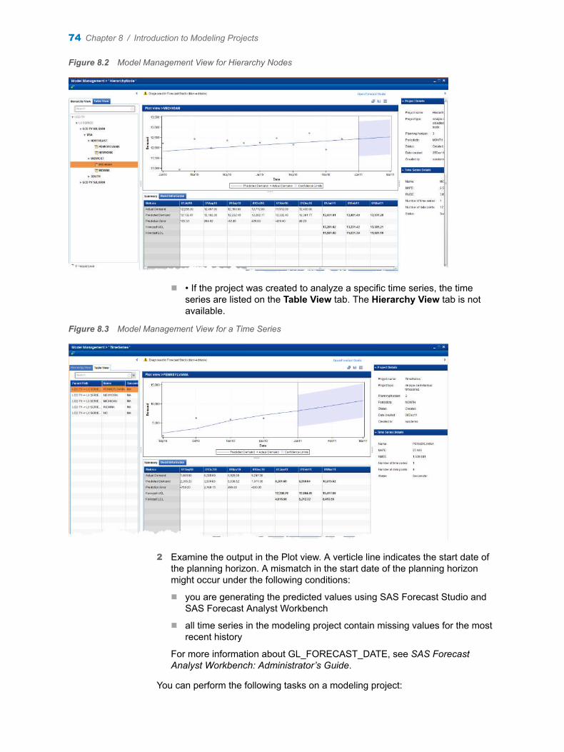
Figure 8.2 Model Management View for Hierarchy Nodes
n • If the project was created to analyze a specific time series, the time series are listed on the Table View tab. The Hierarchy View tab is not available.
Figure 8.3 Model Management View for a Time Series
2 Examine the output in the Plot view. A verticle line indicates the start date of the planning horizon. A mismatch in the start date of the planning horizon might occur under the following conditions:
n you are generating the predicted values using SAS Forecast Studio and SAS Forecast Analyst Workbench
n all time series in the modeling project contain missing values for the most recent history
For more information about GL_FORECAST_DATE, see SAS Forecast Analyst Workbench: Administrator’s Guide.
You can perform the following tasks on a modeling project:
74 Chapter 8 / Introduction to Modeling Projects
n open the project in SAS Forecast Studio to work on improving the forecast accuracy
n promote the modifications included in the project to the linked forecast
n compare the default model with the model that is generated by SAS Forecast Studio
The model with a value of Default in the Source column on the Model Information tab is the model created by SAS Forecast Analyst Workbench. You can see the values generated by the SAS Forecast Studio model by selecting the model with a value of Forecast Server in the Source column.
Status of Modeling Projects
Every project in the Modeling category has a specific status. The following table describes each status.
Table 8.1 Status of Modeling Projects
Status Description
Submitted The modeling project has been submitted for creation.
Created The modeling project and all necessary input tables have been created. This status also indicates that the KPI data has been transferred to SAS Forecast Studio for forecasting and that predicted values have been generated.
Data refreshing in progress
SAS Forecast Analyst Workbench is updating the modeling project data.
Promoted The modeling project has been promoted. The forecast results from SAS Forecast Studio have overwritten the original forecasted values in SAS Forecast Analyst Workbench.
Status of Modeling Projects 75

76 Chapter 8 / Introduction to Modeling Projects
9
Managing Modeling Projects
Guidelines for Modeling Projects . . . . . . . . . . . . . . . . . . . . . . . . . . . . . . . . . . . . . . . . . . . 77
Open SAS Forecast Studio . . . . . . . . . . . . . . . . . . . . . . . . . . . . . . . . . . . . . . . . . . . . . . . . . . 78
Refresh a Modeling Project . . . . . . . . . . . . . . . . . . . . . . . . . . . . . . . . . . . . . . . . . . . . . . . . . 78
Promote a Modeling Project . . . . . . . . . . . . . . . . . . . . . . . . . . . . . . . . . . . . . . . . . . . . . . . . 79
Delete a Modeling Project . . . . . . . . . . . . . . . . . . . . . . . . . . . . . . . . . . . . . . . . . . . . . . . . . . . 79
Guidelines for Modeling Projects
When you are working on a project in SAS Forecast Studio, you must conform to the following guidelines:
n Do not change the hierarchy and variable settings.
n Do not change the periodicity of the modeling project.
n Do not change the forecast horizon for the modeling project.
n Do not change the reconciliation level.
n If you change the model for a time series or add a locked override to the data when it is arranged hierarchically, then reconcile the modeling project.
n Do not give an existing event name to a newly created event.
n Do not delete the modeling project from SAS Forecast Studio.
If you delete a modeling project from SAS Forecast Studio and try to open the same modeling project in SAS Forecast Analyst Workbench, SAS Forecast Analyst Workbench gives an error.
When you promote a locked override from SAS Forecast Studio to SAS Forecast Analyst Workbench, the Do no diagnose option is automatically selected. As a result, the locked override values are retained, even when the forecast is rediagnosed.
When you import the results from the resulting data sets that are in the forecast projects directory into SAS Forecast Analyst Workbench, you can also import the models and events. You can change the parameters other than the periodicity and horizon. However, they are not imported into SAS Forecast Analyst Workbench.
77
You can create scenarios in SAS Forecast Studio. The Model Management view of the Modeling category displays the forecast studio scenario values when you perform the following steps:
1 Model a project for the entire forecast.
2 Create and run the scenarios in SAS Forecast Studio.
3 Set the scenario values as locked override, reconcile the hierarchy, and close SAS Forecast Studio.
4 Refresh the modeling project in the Modeling category.
Open SAS Forecast Studio
The modeling project is created in the Modeling category. You can open a modeling project in SAS Forecast Studio and improve its predicted demand values.
The following prerequisites apply:
n You must have permission to open SAS Forecast Studio. For more information, contact your system administrator.
n In order to launch SAS Forecast Studio using the Java Web Start client, Java Runtime Environment (JRE) 1.7 or later needs to be installed on the client machine.
To open SAS Forecast Studio:
1 In the Modeling category, double-click a project. Alternatively, select a modeling project and click Open. The Model Management view appears.
2 In the Model Management view, click Open Forecast Studio.
SAS Forecast Studio opens and displays the project. For more information, see SAS Forecast Studio: User’s Guide.
Note: When you create a scenario in a modeling project in SAS Forecast Studio, the model forecast values and the scenario forecast values might be different.
Refresh a Modeling Project
You must refresh the modeling project in the Modeling category of SAS Forecast Analyst Workbench to import the changes that you made in SAS Forecast Studio. You must have permission to refresh the modeling project. For more information, contact your system administrator.
To refresh a modeling project, in the Modeling category, select a project and click .
SAS Forecast Analyst Workbench imports all the data related to the modeling project from SAS Forecast Studio. The status of the project changes to Data
78 Chapter 9 / Managing Modeling Projects

refreshing in progress. After the data is imported, the status of the project changes to Created.
Promote a Modeling Project
After you perform advanced tasks related to model management, you can promote the modeling project. When you promote the project, the data associated with the project is merged with the linked forecast in SAS Forecast Analyst Workbench. You must have permission to promote the modeling project. For more information, contact your system administrator.
Suppose you perform advanced model management tasks on a modeling project that contains a new product forecasting time series and then you promote the modeling project. In this case, SAS Forecast Analyst Workbench treats the new product forecasting time series as a regular time series, instead of using the demand that was generated in the New Products workspace.
Suppose the multiple modeling projects are linked to the same forecast and you want to promote those modeling projects. In such a case, promote one modeling project at a time, and then wait for the status of the forecast to change from Obtaining modeling project data to Forecasted before you promote the next modeling project.
To promote the modeling project:
1 In the Modeling category, select a project and click . The Promote window appears.
2 Choose the appropriate options.
Note: You cannot clear the Models check box because the models that are created in SAS Forecast Studio are always promoted to the selected forecast.
3 Click OK.
SAS Forecast Analyst Workbench starts promoting the modeling project and changes the status to Promoting. After the predictions in the forecast have been overwritten with the data from the modeling project, the status of the project changes to Promoted.
After you promote the modeling project, the model that was applied in the modeling project becomes the default model for the forecast
4 Reconcile the forecast in order to update the predicted values.
For more information about reconciliation, see “Reconcile a Forecast” on page 57.
Delete a Modeling Project
You must have permission to delete a modeling project. For more information about permissions, contact your system administrator.
To delete a modeling project:
Delete a Modeling Project 79

1 In the Modeling category, select a project, and click .
2 In the confirmation window, click Yes.
The selected modeling project is deleted. All associated tables and data that were created for the project are also deleted.
80 Chapter 9 / Managing Modeling Projects

Part 5Forecasting a New Product
Chapter 10Forecasting a New Product . . . . . . . . . . . . . . . . . . . . . . . . . . . . . . . . . . . . . . . . 83
81

82

10
Forecasting a New Product
Overview of Forecasting a New Product . . . . . . . . . . . . . . . . . . . . . . . . . . . . . . . . . . . . 83
Workflow for Forecasting a New Product . . . . . . . . . . . . . . . . . . . . . . . . . . . . . . . . . . . . 84
Create a New Product Forecast Project . . . . . . . . . . . . . . . . . . . . . . . . . . . . . . . . . . . . . 86
View Details of a New Product Forecast Project . . . . . . . . . . . . . . . . . . . . . . . . . . . . . 88
Define Relationships and Candidate Products . . . . . . . . . . . . . . . . . . . . . . . . . . . . . . 88
Select Candidate Products and Adjust Seasonality . . . . . . . . . . . . . . . . . . . . . . . . . . 89
Select Surrogate Products . . . . . . . . . . . . . . . . . . . . . . . . . . . . . . . . . . . . . . . . . . . . . . . . . . 91
Select a Model . . . . . . . . . . . . . . . . . . . . . . . . . . . . . . . . . . . . . . . . . . . . . . . . . . . . . . . . . . . . . . 92
Review the Forecast . . . . . . . . . . . . . . . . . . . . . . . . . . . . . . . . . . . . . . . . . . . . . . . . . . . . . . . . 93
Assigning New Product Forecast Projects to a Forecast . . . . . . . . . . . . . . . . . . . . 94About Assigning New Product Forecast Projects to a Forecast . . . . . . . . . . . . . . . 94Assign a New Product Forecast Project to a Forecast . . . . . . . . . . . . . . . . . . . . . . . 95
Delete a New Product Forecast Project . . . . . . . . . . . . . . . . . . . . . . . . . . . . . . . . . . . . . . 96
Statuses of a New Product Forecast Project . . . . . . . . . . . . . . . . . . . . . . . . . . . . . . . . 96
Overview of Forecasting a New Product
SAS Forecast Analyst Workbench enables you to use a structured judgment process that combines statistical analysis and judgmental analysis methods to generate the forecasted values for the new product. You can generate the forecasted values for any key performance indicator, such as demand or sales. The new product forecasting process helps you overcome the following challenges that are involved in forecasting the demand for a new product:
n lack of product history
n uncertain product life cycle
SAS Forecast Analyst Workbench enables you to accomplish the following goals:
n leverage your business or domain knowledge by using a structured judgment technique
n combine business judgment with statistical techniques to calculate the history of surrogate products
83

n construct an appropriate model based on the history of surrogate products in order to generate forecasts of the new product that can be reviewed easily
Workflow for Forecasting a New Product
SAS Forecast Analyst Workbench uses the following systematic workflow to forecast values for new products.
1 Create a new product forecast project.
The project contains the new product and its parameters such as KPI, periodicity, number of clusters to be created, and so on.
For more information about creating a new product forecast project, see “Create a New Product Forecast Project” on page 86.
2 Define the relationship of the new product to the non-product dimensions, and define candidate products.
In this step, you define the applicability of your product. You can define the relationship between the new product and the non—product dimensions that are defined for the selected KPI. For example, if you are introducing the new product in a particular region of the USA, you subset the members in the Location dimension for that region.
You also select products whose historical demand data can be used to forecast the new product. These products are called candidate products. You can also specify common attributes and attributes that are specific to the new product to filter the candidate products. SAS Forecast Analyst Workbench uses the historical demand data of the candidate products to subset the specified non-product dimensions. For example, if you specified that a new product will be launched in the Northeast, only the historical data of the candidate products in the Northeast are used to create the new product forecast.
SAS Forecast Analyst Workbench uses the relationship of the new product with the dimensions to generate the demand history for the selected candidate products. For example, SAS Forecast Analyst Workbench retrieves the demand history that is available for cell phone 1 and cell phone 2 in California if you selected only California in the Location dimension and specified cell phone 1 and cell phone 2 as the candidate products. The historical demand data of these candidate products is used to generate the forecast for the new product.
For more information about defining the relationship of the product to the dimensions and defining candidate products, see “Define Relationships and Candidate Products” on page 88.
3 Select candidate products and analyze the seasonality of the candidate products.
You select a set of candidate products whose statistical properties are similar to the new product. Because the new product series is not known, you can use the known attributes of the new product to find a set of candidate products with similar attributes. You can graphically view a set of the candidate series that is associated with the candidate products. After you view the candidate products, use your judgment to remove one or more
84 Chapter 10 / Forecasting a New Product

candidate products. Then you can graphically explore the revised set of candidate products to better understand the impact of your changes. You might want to keep products that were launched during the same season as the new product. Using your business judgment, remove outlier products whose demand pattern is not likely to be similar to the expected demand pattern of the new product. SAS Forecast Analyst Workbench creates clusters of the remaining candidate products that have a similar demand pattern. Each cluster contains the candidate products that can be used for modeling and forecasting the values of the new product.
For more information about selecting candidate products, see “Select Candidate Products and Adjust Seasonality” on page 89.
4 Select a cluster that contains the most suitable candidate products. The historical data of these candidate products is used to apply the statistical models. The candidate products in this cluster become surrogate products for the new product.
When you select surrogate products, the following processes occur:
n analysis of the statistical pattern of the demand of the candidate products
n filtering of the outlier products from the list of candidate products
To create the clusters, SAS Forecast Analyst Workbench uses the reduction method that you selected when you created the new product forecast project. Each cluster contains the candidate products that have similar demand patterns. You remove the outlier products from the set of candidate products that was returned in the previous step. If you correctly remove the outlier series, then the set of surrogate series should be more similar to the new product series than the set of candidate series was.
For more information about selecting surrogate products, see “Select Surrogate Products” on page 91.
5 Apply models and generate the predicted demand for the new product.
SAS Forecast Analyst Workbench applies the Naive and Neural models to the surrogate products of the cluster that you selected. In this step, you extract the statistical features from the set of surrogate products. These surrogate products are similar to the new product series and are useful for forecasting the new series. After you select a model, it is fitted to the surrogate products and prediction errors are computed. You can graphically explore the set of surrogate products, and manipulate the statistical model that is applied.
For more information about selecting a model, see “Select a Model” on page 92.
6 (Optional) Using your judgment of various factors (such as market conditions, organizational environment, constraints, and so on), review the forecast and override the predicted demand.
This step predicts the new product series by using the historical launch data that is associated with the surrogate products. After you explore the forecasts, you might decide to override the statistical predictions. For example, you can override the forecasts for the profile series, the total quantity, or the cycle series. You can then graphically explore statistical forecasts and overrides to better understand the impact of your changes. If you override the predicted demand, SAS Forecast Analyst Workbench marks the demand values as the final forecasted values.
Workflow for Forecasting a New Product 85

For more information about reviewing the forecasted demand values, see “Review the Forecast” on page 93.
7 Assign the project to a forecast. You can view the demand in the Model Management view.
For more information about assigning the New Product Forecasting project to a forecast, see “Assigning New Product Forecast Projects to a Forecast” on page 94.
Create a New Product Forecast Project
You must create a new product forecast project in order to forecast the demand for that new product. A new product forecast project consists of the new product and its parameters, such as key performance indicator (KPI), periodicity or forecasting interval, and so on. You must have permission and data authorization to create a new product forecast project. For more information, see SAS Forecast Analyst Workbench 5.3: Administrator’s Guide. Alternatively, contact your system administrator.
To create a new product forecast project:
1 In the New Products workspace, click the NPF Projects category, and then click . The New Product Forecast Project view appears.
2 In the Select Product section, select a new product.
3 In the Select Parameters section, enter information in each field. The following table describes each field.
Table 10.1 Field Descriptions for the Select Parameters Section
Field Description
KPI Select the key performance indicator (KPI). The KPI is the variable that is to be forecasted for the new product. For example, select Demand to forecast the demand for the new product.
Periodicity Select the periodicity. The periodicity defines the forecasting interval or the frequency at which the demand should be forecasted.
86 Chapter 10 / Forecasting a New Product

Field Description
Number of cycles
Enter the number of cycles of the candidate products that you want to consider for generating the forecast results of the new product. A cycle is a period of time whose length is defined by your periodicity. The first cycle begins at the introduction of the candidate product. The next cycle begins on the date following the previous cycle. Cycle series data is useful for modeling and for comparing time series data with different introduction times. SAS Forecast Analyst Workbench considers the earliest demand that is available for the specified number of cycles of the candidate products.
For example, if you selected Month in the Periodicity list, and you entered 12 in the Number of cycles field, SAS Forecast Analyst Workbench considers the demand that was generated during the first 12 months after the launch of the candidate products.
Number of clusters
Enter the number of clusters that SAS Forecast Analyst Workbench must create. The clusters group the candidate products with similar demand pattern together.
Reduction method
Select the reduction method in order to reduce each candidate series to a uniform set of statistical properties that are not time-dependent. The list contains the following options:n Decomposition: Select this option to analyze seasonal
patterns. You can use this option when at least two seasonal cycles of the time series data are available.
n Smoothing: Select this option to obtain level and trend estimates of the candidate products.
Sales introduction date
Displays the sales introduction date of the new product. Click to change the date.
Note: SAS Forecast Analyst Workbench does not convert the time zone automatically if the SAS Forecast Analyst Workbench server and client are located in different time zones. You must perform the GMT time zone conversion manually before you enter the sales introduction date.
Hierarchy path Displays the path where the new product fits into the product hierarchy. This path helps you locate the new product easily in the Model Management view.
4 Click OK.
Note: You can create one new product forecast project for each combination of the new product and the KPI.
SAS Forecast Analyst Workbench closes the New Product Forecast Project view and creates the project with the status Ready for NPF. You can start the process of forecasting the demand values for this new product.
Create a New Product Forecast Project 87

View Details of a New Product Forecast Project
You use the New Product Forecast Project view to forecast the new product. The New Product Forecast Project view is divided into two parts. The upper part of the view displays the steps of the new product forecasting process. After you complete each step, a appears at the bottom of the process step, which indicates that the step is complete. The bottom part of the view displays the options for the selected step and the result of the process.
You cannot proceed to the next step of the process unless you have completed the previous step. However, you can click a rectangle that contains to view and change the options for that step. These steps help you maintain a consistent and structured workflow for forecasting the values of the KPI for the new product.
Figure 10.1 NPF Process Flow
Define Relationships and Candidate Products
TIP In this step, you should identify a forecast to which you will promote this new product forecasting project after you obtain the demand for the new product.
To define relationships and candidate products:
1 In the New Products workspace, click the NPF Projects category, and double-click a project that is in the Ready for NPF state. The New Product Forecast Project view appears and contains two panes. The name of the right pane changes depending on the option that you select in the left pane.
2 Define the relationship of the new product with the non-product dimensions.
a In the left pane, click Relationships. The Select domain relationships pane displays all the non-product dimensions on separate tabs.
b Select at least one value on each tab.
For example, if you are introducing the new product in a particular region of the USA, select only that region on the Location tab.
3 Define the candidate products whose historical data can be used to forecast the new product.
88 Chapter 10 / Forecasting a New Product

a In the left pane, click Candidate Products. The right pane displays two sections: Available items and Selected items.
b In the Available items section, select the candidate products. The candidate products are arranged in a tree structure. You can expand and collapse the hierarchy to select the candidate products.
c Click . The hierarchy of the selected candidate products appears in the Selected items section.
d (Optional) Click Common attributes to define common attributes.
Note: This link is available only if common attributes are defined for the selected hierarchical values.
e (Optional) Click Product-specific attributes to define product-specific attributes of the new product.
By specifying product-specific attributes, you can filter the candidate products that are most suitable.
Note: This link is available only if product-specific attributes are defined for the selected hierarchical values.
4 Click OK.
SAS Forecast Analyst Workbench retrieves, subsets, and aggregates the historical data for the defined candidate products for the selected dimensions. SAS Forecast Analyst Workbench uses this data to forecast the new product.
The state of the new product forecast project changes from Ready for NPF to Data population completed.
Select Candidate Products and Adjust Seasonality
You can select the candidate products that are useful in forecasting the demand for the new product. The new product forecast project must be in the Data population completed state.
To select the candidate products:
1 In the New Products workspace, click the NPF Projects category, and double-click a project. The New Product Forecast Project view appears. The left pane displays a list of candidate products in different colors. The right pane contains a histogram, KPI plot, KPI percent plot, and time series plot on separate tabs.
For more information about the plots that are displayed, see
2 View the information about candidate products by using the histogram, KPI plot, KPI percent plot, time series plot.
n Use histogram to view a graphical representation of the distribution of data. A histogram consists of tabular frequencies, shown as adjacent rectangles, erected over discrete intervals (bins). The x-axis displays the total KPI value over the total number of cycles for the candidate products. If the KPI is demand and the project was set up to create a new product
Select Candidate Products and Adjust Seasonality 89

forecast for the first 20 weeks, the x-axis displays the total demand for candidate products during the first 20 weeks after their launch. The y-axis displays the percentage of candidates that fall within each interval of total demand.
n Use KPI plot for removing outlier products from the list of candidate products. The name of the plot depends on the KPI that you selected. For example, if you selected Demand, SAS Forecast Analyst Workbench displays the name of the plot as Demand Plot. The KPI plot displays the historical values of the selected candidate products in different cycles. The x-axis displays the cycle index, and the y-axis displays the historical value for a candidate product during that cycle. You can observe the historical values of the outlier product to remove it from the list of the candidate products.
n Use the KPI percent plot to view the historical values of the selected candidate products as percentages. The name of the plot depends on the KPI that you select. For example, if you select Sales, SAS Forecast Analyst Workbench displays the name of the plot as Sale Percent Plot. This plot helps you analyze the historical values of the candidate products against the cycle index. The x-axis displays the cycle index, and the y-axis displays the historical values of the candidate products, as percentages.
n Use the time series plot to view the historical demand for the candidate products against the date. Each line in this graph denotes the actual demand data for each candidate product in its original time period. Thus, the graph of each candidate product can start at a different date.Because the demand for each candidate product is displayed against its actual time, the time series plot helps you understand the seasonal pattern of the candidate products. If the candidate products show seasonal fluctuations, you might decide to adjust their seasonality. The time series plot enables you to view the data for a particular time series and for particular durations. For example, you can view the data for the first seven time series between January 2010 and December 2010.
You can select the candidate products and then filter their demand data. For example, you might want to view the demand data of only two candidate products out of four candidate products.
You can filter the data in the plot by selecting a time range for which you want to view data. For example, you might want to view the demand data that was generated from March to November.
Note: If all time series contain the value 0 for a particular date, change NPF_MODE to ADD in the configuration table. For more information, contact your Administrator.
3 (Optional) Click Reset graph to reset the time series and duration in the time series plot.
90 Chapter 10 / Forecasting a New Product

4 Clear the check box of the candidate product that is an outlier. You can now explore the historical demand data of the candidate products using the different plots.
Note: Whenever you select or remove a candidate product, click Refresh to refresh the data on the plots.
5 (Optional) Select the Adjust seasonality check box to remove the seasonality patterns from the data for the candidate products.
You can adjust the seasonality if the candidate products display regular seasonal fluctuations.
Note: This check box is available only when the selected candidate products contain at least two periods of data.
TIP When you want to adjust seasonality, ensue that the candidate products contain sufficient data for the selected cycles.
6 (Optional) Click Refresh to refresh the histogram, KPI plot, KPI percent plot, and time series plot.
Note: If you click Refresh after you adjust the seasonality, the histogram, KPI plot, and KPI percent plot display the de-seasonalized data. However, the time series plot does not display the de-seasonalized data.
7 Click OK.
SAS Forecast Analyst Workbench removes the outlier products that you selected from the set of the candidate products and forms the clusters based on the time series pattern of the remaining candidate products. The state of the new product forecast project changes from Data population completed to Clustered.
Select Surrogate Products
The new product forecast project must be in the Clustered state before you can select surrogate products.
To select surrogate products:
1 In the New Products workspace, click the NPF Projects category and double-click a project. The New Product Forecast Project view appears.
2 In the Select Cluster list, select a cluster. The cluster graph and the cluster table display the historical demand data of the surrogate products in percentages, arranged against different cycles.
3 Explore the number of surrogate products in a cluster to ensure that sufficient surrogate products are present.
4 (Optional) Use your judgment and clear the check box next to one or more surrogate products to remove them from the cluster.
The cluster graph refreshes and displays the updated data. You can graphically explore the revised set of surrogate products to better understand the impact of judgments.
Select Surrogate Products 91

5 Repeat steps 2 through 4 to select the cluster that is most suitable for your needs.
6 Click OK.
SAS Forecast Analyst Workbench starts fitting the Naive and Neural models to the surrogate products of the selected cluster. You can also use a custom model. Detailed information about how to set up a custom model is in SAS Forecast Analyst Workbench: Administrator’s Guide.
After the models are fitted, SAS Forecast Analyst Workbench generates the predicted demand for the new product by using the demand of the surrogate products of the selected cluster. The state of the new product forecast project changes from Clustered to Modeled.
Select a Model
You can select the model that is most suitable for the new product. The new product forecast project must be in the Modeled state.
To select a model:
1 In the New Products workspace, click the NPF Projects category, and double-click a project. The New Product Forecast Project view appears.
2 In the Select model list, select a model.
The Model Summary, Profile Series Model, and Cycle Series Model tabs display the graphs of the predicted demand of the new product.
3 View information about the model and predicted demand of the new product by using the mean absolute percentage error (MAPE), root mean square error (RMSE), Akaike information criterion (AIC), and adjusted R-square in the following tabs:
n Use the Model Summary tab to view the overall prediction, regardless of the cycle ID. The Model Summary tab displays a histogram of the percentage of surrogate products that are within a particular range of the total demand.
n Use the Profile Series Model tab to view the percentage of the predicted value of the new product for different cycles.
n Use the Cycle Series Model tab to view the predicted demand for each candidate product in each cycle.
4 (Optional) Use your judgment and clear the check box that is next to one or more products that are outliers to remove them from the list of surrogate products.
For example, you might select or remove poorly fitting surrogate (outlier) series or choose other model specifications.
Note: Whenever you select or remove any product from the list of the surrogate products, click Refresh to update the graphs.
5 Repeat steps 2 through 4 to select a model that is the most suitable for your needs.
92 Chapter 10 / Forecasting a New Product

6 (Optional) If you are not satisfied with the predicted demand after choosing the model, you can go back to the Select Cluster step.
7 Click OK.
SAS Forecast Analyst Workbench applies the selected model to the surrogate products and generates the predicted demand values for the new product. The state of the new product forecast project changes from Modeled to Forecasted.
If you specified to adjust for seasonality when you selected the candidate products, SAS Forecast Analyst Workbench readjusts the predicted demand of the new product for seasonality.
Review the Forecast
After you explore the forecasts, you might decide to override the statistical predictions. For example, you can override the forecasts for the profile series, the total quantity, or the cycle series. After you apply judgment, you can graphically explore statistical forecasts and judgmental overrides to better understand the impact of your changes. For example, you might explore the impact of overrides within the context of the statistical forecasts (predictions and confidence limits). You can review and override the predicted demand value of the new product to make it the final forecast. The new product forecast project must be in the Forecasted state.
To review the forecast:
1 In the New Products workspace, click the NPF Projects category and double-click a project. The New Product Forecast Project view appears.
2 On the Cycle Series tab and the Profile Series tab, review the predicted demand values.
n The Cycle Series tab displays the predicted demand values of the new product for all cycles.
n The Profile Series tab displays the predicted demand values of the new product, as a percentage, for all cycles. It also displays these values in tabular form.
3 To override the demand values, enter new values:
n On the Cycle Series tab, in the table of demand values, enter a new demand value in the cell of any cycle to override it manually. When you override the demand value on the Cycle Series tab, SAS Forecast Analyst Workbench changes the total predicted demand in the Demand Summary table and the percentage of all cycles on the Profile Series tab.
n On the Profile Series tab, in the table of demand values, enter a new percentage value in the cell of any cycle to override its demand value manually. The predicted demand is shown up to four decimal points. When you override the demand value on the Profile Series tab, SAS Forecast Analyst Workbench changes the predicted demand values of all cycles on the Cycle Series tab and the percentage of all cycles on the Profile Series tab. SAS Forecast Analyst Workbench retains the total predicted demand value.
Review the Forecast 93

Note: When an override value is available, that value is saved as the final forecast. Otherwise, the original predicted value is saved as the final forecast. You cannot enter negative values.
4 (Optional) If you are not satisfied with the override values, click Reset. SAS Forecast Analyst Workbench resets the demand values to the original values.
5 (Optional) Repeat steps 2 through 4 to perform different scenarios.
6 After you are satisfied with the demand values, click Close.
If you are not satisfied with your results, you can select a different model. (See “Select a Model” on page 92.)
SAS Forecast Analyst Workbench replaces the final forecast values, either with the override values, if those are available, or with the predicted values. The state of the new product forecast project changes to NPF completed. Now, you can assign this project to a forecast.
Assigning New Product Forecast Projects to a Forecast
About Assigning New Product Forecast Projects to a Forecast
You can assign the new product forecast project to a forecast if the following conditions are true:
n the forecast and the new product forecast project contain the same KPI
n when you created the forecast, you selected the leaf level of the Product dimension at or above the forecast-leaf-level on the Reorganize Hierarchy page
You can assign the new product forecast project to multiple forecasts.
When you assign the new product forecast project to a forecast and a mismatch in the periodicity occurs, SAS Forecast Analyst Workbench automatically performs the conversion of the new product forecast project demand according to the forecast periodicity values. In other words, even if the forecast is at a more granular periodicity, new product forecasts can be accommodated in the forecast.
For example, if the periodicity of the new product forecast project is month but the forecast periodicity is weekSAS Forecast Analyst Workbench converts the monthly values of the new product forecast project to weekly values to fit them in the forecast.
When you assign the new product forecast project to a forecast, SAS Forecast Analyst Workbench overrides the statistical forecast values with the values that are obtained from the new product forecasting process. The forecasted values before the horizon start date for the new product time series might be missing.
When you perform the following sequence of tasks on a forecast, the statistical forecast values of the new product time series are replaced by the new product forecast project values:
94 Chapter 10 / Forecasting a New Product

1 create a modeling project, perform modeling tasks, and then promote the modeling project to the forecast in order to obtain the values from SAS Forecast Studio
2 create and then promote a new product forecast project to the forecast
When you perform the following sequence of tasks on a forecast, the statistical forecast values of the new product time series are replaced by the values obtained from the modeling project:
1 create and then promote a new product forecast project to the forecast
2 create a modeling project, perform advanced modeling tasks in SAS Forecast Studio, and then promote the modeling project to the forecast in order to obtain the values from SAS Forecast Studio
In other words, SAS Forecast Analyst Workbench retains the forecast values obtained from the last action that you perform on a forecast.
If the horizon end date of the new product forecast project is equal to or less than that of the forecast, SAS Forecast Analyst Workbench takes the values of the new product time series from the new product forecasting process in the forecast until the horizon end date of the new product forecast project.
If the horizon end date of the new product forecast project is greater than that of the forecast, SAS Forecast Analyst Workbench takes the values of the new product time series from the new product forecasting process in the forecast until the horizon end date of the forecast. As the incremental data becomes available for the forecast, the forecast horizon end date proceeds. In such case, SAS Forecast Analyst Workbench takes the next incremental data from new product forecast project for the new product time series until the horizon end date of the new product forecast project.
For example, the horizon end date for the forecast is Nov 2015 and the horizon end date for new product forecast project is Mar 2016. During the first cycle of running the forecast in a monthly batch, SAS Forecast Analyst Workbench takes the data until Nov 2015 in the forecast from new product forecast project. During the next cycle of the batch run, SAS Forecast Analyst Workbench takes the data until Dec 2015 from new product forecast project and so on. This process continues until the forecast horizon end date reaches to Mar 2016.
When the historical data for the new product becomes available, SAS Forecast Analyst Workbench will treat the new product as a regular product and generate a statistical forecast based on the history.
Assign a New Product Forecast Project to a Forecast
The following prerequisites apply:
n You must have permission to assign a new product forecast project to a forecast. For more information, contact your system administrator.
n The new product forecast project must be in either the NPF completed or Forecasted state.
n The forecast must be in either the Forecasted or Accepted state.
n The horizon start date and end date for the new product forecasting project and for the forecast must overlap.
To assign a new product forecast project to a forecast:
Assigning New Product Forecast Projects to a Forecast 95

1 In the New Products workspace, click the NPF Projects category and select a project.
2 Click . The Assign to Forecasts window displays a list of forecasts that have the same KPI.
Note: The list of forecasts does not include forecasts to which you have already assigned this new product forecast project. If you re-create a forecast after you have assigned the new product forecast project to that forecast, the forecast appears in the list of available forecasts.
3 Select one or more forecasts, and click OK.
After you click OK, SAS Forecast Analyst Workbench starts integrating the data of the new product forecasting project with a forecast and changes the status of the forecast to Obtaining NPF data. After the data of a new product forecasting project is integrated completely with a forecast, the status of the forecast becomes Forecasted.
After you assign a new product forecasting project to a forecast, the status of the new product forecasting project remains the same, that is, either Forecasted or NPF Completed.
Delete a New Product Forecast Project
If you delete a new product forecast project that is assigned to a forecast, the forecast continues to use the forecast values that the new product forecast project generated for the new product.
The following prerequisites apply:
n You must have permission to delete a new product forecast project. For more information, contact you system administrator.
n The new product forecast project must not be in a state that is in progress.
To delete a new product forecast project:
1 In the New Products workspace, select a project and click .
Note: You cannot delete multiple projects simultaneously.
2 In the confirmation window, click Yes.
The selected new product forecast project and its data are removed from SAS Forecast Analyst Workbench.
Statuses of a New Product Forecast Project
The following table provides a list of the status of a new product forecast project.
96 Chapter 10 / Forecasting a New Product

Table 10.2 Statuses of New Product Forecasting Projects
Status Description
Ready for NPF The new product forecast project has been created. You can double-click the project to open it and perform additional tasks.
Data population in progress
The new product forecast project is being created, and SAS Forecast Analyst Workbench is calculating the data.
Error in data population
An error occurred in calculating the data for the new product forecasting project.
Data population completed
The candidate products have been defined. The relationships between the new product and the non-product dimensions of the forecast have also been defined.
Clustering in progress
SAS Forecast Analyst Workbench is creating clusters based on the settings that you defined when you created the new product forecasting project.
Clustered The candidate products have been selected and clusters have been created.
Error in clustering
An error occurred when the clusters were created.
Modeling in progress
The surrogate products are being selected and a new product forecast is being created using each of the available models.
Modeled The surrogate products have been selected and a new product forecast is created using each of the available models.
Error in modeling
An error occurred when the surrogate products were selected.
Forecasting in progress
The selected statistical model is being applied to the surrogate products, and the predicted demand values are being generated.
Forecasted The selected statistical model has been applied to the surrogate products, and predicted demand values have been generated.
Error in forecasting
An error occurred in applying the model and generating the predicted demand values.
NPF completed The predicted values of the new product have been reviewed and finalized.
Deleting NPF project
The new product forecasting project is being deleted.
Error in deleting NPF project
An error occurred in deleting the new product forecasting project.
Error: Insufficient data
SAS Forecast Analyst Workbench does not contain sufficient data to create the new product forecast project.
Statuses of a New Product Forecast Project 97

98 Chapter 10 / Forecasting a New Product

Part 6Performing Custom Analyses
Chapter 11Performing Custom Analyses . . . . . . . . . . . . . . . . . . . . . . . . . . . . . . . . . . . . . 101
99

100
11
Performing Custom Analyses
Introduction to Performing Custom Analysis . . . . . . . . . . . . . . . . . . . . . . . . . . . . . . 101
Workflow for Using Custom Analysis . . . . . . . . . . . . . . . . . . . . . . . . . . . . . . . . . . . . . . 101
Create an Analysis . . . . . . . . . . . . . . . . . . . . . . . . . . . . . . . . . . . . . . . . . . . . . . . . . . . . . . . . 102
Use the Three-Stage Modeling Analysis . . . . . . . . . . . . . . . . . . . . . . . . . . . . . . . . . . . 103
Edit an Analysis . . . . . . . . . . . . . . . . . . . . . . . . . . . . . . . . . . . . . . . . . . . . . . . . . . . . . . . . . . . 105
Share an Analysis with Another User . . . . . . . . . . . . . . . . . . . . . . . . . . . . . . . . . . . . . . 105
Delete an Analysis . . . . . . . . . . . . . . . . . . . . . . . . . . . . . . . . . . . . . . . . . . . . . . . . . . . . . . . . . 106
Explore the Output of the Analysis . . . . . . . . . . . . . . . . . . . . . . . . . . . . . . . . . . . . . . . . 106
Introduction to Performing Custom Analysis
SAS Forecast Analyst Workbench enables SAS consultants and analysts to write SAS Stored Processes as custom analyses. You can use the custom analyses to improve the quality of the forecast or whenever you want to use custom methods of forecasting that meet your business requirements. You can use the predicted values that are generated from custom analyses in the downward processes of supply-chain management. You can integrate the output of custom analysis with SAS Collaboration Planning Workbench for collaboration planning and with SAS Inventory Optimization Workbench for optimizing the inventory.
Workflow for Using Custom Analysis
Use the following workflow to perform custom analysis:
1 Write a SAS Stored Process that meets your business requirements, and then save the SAS Stored Process. You must be a SAS consultant to write a stored process.
You can use the template located at SASHome\SASFoundation\9.4\ddcfsrv\sasstp\ddcf_ca_stp_template.sas to write the SAS
101

Stored Process. Then, copy that file to the following location: SASHome\SASFoundation\9.4\ddcfsrv\sasstp.
For more information, see SAS Forecast Analyst Workbench: System Administrator’s Guide.
2 Register the SAS Stored Process in SAS Management Console. You must be a SAS consultant or administrator to register the stored process.
For more information about registering the SAS Stored Process, see SAS Forecast Analyst Workbench: System Administrator’s Guide.
3 In SAS Forecast Analyst Workbench, create an analysis and run it in order to generate the output.
4 (Optional) Explore the output of the custom analysis by creating a report in SAS Visual Analytics.
For more information about creating a report in SAS Visual Analytics, see Chapter 18, “Working with Reports,” on page 159.
5 (Optional) When the incremental historical data is added to the forecast, edit the custom analysis and then rerun it in order to obtain predicted values based on the latest data.
6 Use the output of the custom analysis in the downward processes of supply-chain management, such as collaboration planning and integrating with SAS Inventory Optimization Workbench.
For more information about integrating the output of custom analysis with collaboration planning, see “Create a Plan” on page 113.
For more information about integrating the output of custom analysis with SAS Inventory Optimization Workbench, see SAS Inventory Optimization Workbench: User’s Guide.
Create an Analysis
Use the SAS Stored Process that you have already created to create a custom analysis. You must have permission to create an analysis.
The following prerequisites apply:
n The forecast that you want to use for analysis must be in one of the following states: Created, Forecasted, or Accepted.
n A SAS consultant must write code for the analysis and register the SAS Stored Process in SAS Management Console. For more information about writing code for analysis and registering the SAS Stored Process, see SAS Forecast Analyst Workbench: Administrator’s Guide.
To create an analysis:
1 In the Analysis workspace, click . The Analysis wizard appears.
2 In the Identification step of the Analysis wizard, enter a name and description for the analysis.
102 Chapter 11 / Performing Custom Analyses

Note: The analysis name must be unique and must be a valid SAS name. For more information about SAS naming conventions, see SAS Language Reference: Concepts at https://support.sas.com/documentation/cdl/en/lrcon/69852/HTML/default/viewer.htm.
3 In the Select analysis field, click Browse to select an analysis.
You can select the Three Stage Modeling analysis to perform the analysis on SAS 9.4, or select the Three Stage Modeling Viya analysis to perform the analysis on SAS Viya. For more information about three-stage modeling analysis, see “Use the Three-Stage Modeling Analysis” on page 103.
4 Click Next to proceed.
5 In the Obtain Available Forecasts step, click Run and Save Step to obtain the forecasts that are available to you.
A list of all available forecasts is displayed. You can perform the analysis on any of the available forecasts.
6 Click Next to proceed.
7 Based on the analysis that you selected in Step 3 on page 103, you might need to complete additional steps (such as selecting input parameters, forecast, and so on). Select any required values, and then click Run and Save Step for each step.
SAS Forecast Analyst Workbench displays the result of each step on the Output tab. You can also view the log for the process on the Log tab.
8 When you have completed all the steps in theAnalysis wizard , click Finish.
The status of the analysis changes to Complete. SAS Forecast Analyst Workbench stores the output of the analysis at the location that is specified in the SAS Stored Process.
You can create a report in SAS Visual Analytics to explore the predicted values. If the output of analysis is satisfactory, you can use the output in the downward processes of supply-chain management, such as integrating with SAS Inventory Optimization Workbench and performing collaboration planning.
Use the Three-Stage Modeling Analysis
The three-stage modeling analysis is an out-of-the-box analysis that you can use as a template for an analysis that you want to perform. You can perform the three-stage modeling analysis on SAS 9.4 or on SAS Viya.
When you are performing a three-stage modeling analysis, the following prerequisites apply:
n the forecast must contain at least one independent variable
n the historical and future values of all independent variables that you select in the forecast for the entire horizon must be available in order to generate predicted values
If the historical or future values of any of the independent variables are missing, you must set an appropriate option on the DIAG_INPUT_SETMISSING<n> parameter in the
Use the Three-Stage Modeling Analysis 103

CONFIG.HPF_PREFERENCES<plan_id> table for the independent variable. For more information about the option, the DIAG_INPUT_SETMISSING<n> parameter, and the CONFIG.HPF_PREFERENCES<plan_id> table, see SAS Forecast Analyst Workbench: Administrator's Guide.
Consider using two seasons worth of data to obtain more accurate predicted values in the three-stage modeling analysis. For example, suppose you want to predict the demand for XYZ product in July 2017. In this case, consider using the data from July 2015.
When the analysis is performed on SAS Viya, PROC TSMODEL and PROC REGSELECT are used.
Use the following parameters to perform three-stage modeling analysis:
Table 11.1 Input Parameters for Three-Stage Modeling Analysis
Parameter Description
Forecast Select the name of the forecast that you want to use for three-stage modeling.
Selection method Select one of the selection methods.
Criterion Select the criterion that SAS Forecast Analyst Workbench will use to select the best model.
Confidence level (%) Select the confidence level to use for the construction of confidence intervals.
Holdout percent (%) Specify the size of the holdout sample as a percentage of the length of the time series.
The output of the three-stage modeling analysis is saved in the table called ca_outfor_<prj_def_no> in the forecast-specific tables directory. In other words, the ca_outfor_<prj_def_no> table is present in a location that is derived from the path that is specified in the GL_DATA_STORAGE_PATH configuration parameter and by the forecast-specific data in the HPF folder. You can obtain the the value for <prj_def_no> from the UIART.RPT_PROJECT_DEF and UIART.RPT_DEF_NO tables.
For example, suppose the following information is associated with a particular three-stage modeling analysis:
n The path specified in the GL_DATA_STORAGE_PATH configuration parameter is C:\SAS\Config\Lev1\AppData\SASForecastAnalystWorkbench\data.
n The granularity of the forecast is DAY.
n The name of the forecast is Sample.
n The project definition number for the custom analysis is 14.
n the forecast contained only one leaf level in the hierarchy for store location, which is Downtown Detroit
In this case, the ca_outfor_<prj_def_no> table is present in each hierarchical folder in C:\SAS\Config\Lev1\AppData\SASForecastAnalystWorkbench\data\HPF\DAY\Sample\Store_Location_RK\ca_outfor_14.
104 Chapter 11 / Performing Custom Analyses
In addition to using three-stage modeling as an out-of-the-box analysis, you can modify the code for the modeling based on your business requirements. On Windows, the code for three-stage modeling analysis is located at SASHome\SASFoundation\9.4\ddcfsrv\sasmisc\ddcf_ca_3_stg_modeling_code.sas. On UNIX, the code for three-stage modeling analysis is located at SASHome/SASFoundation/9.4/misc/ddcfsrv/ddcf_ca_3_stg_modeling_code.sas.
Edit an Analysis
You can modify the parameters of an analysis and change the type of the analysis.
When a forecast is refreshed, incremental historical data is added to the forecast. After the refresh, you can edit and then rerun the analysis so that SAS Forecast Analyst Workbench generates the predicted values using the latest historical data for the forecast.
The following prerequisites apply to editing an analysis:
n You must have permission to edit an analysis. For more information, contact your system administrator.
n The analysis must not be in the In Progress state.
To edit an analysis:
1 In the Analysis workspace, select an analysis, and then click . The Analysis wizard appears.
2 For each step in the wizard, edit the required details, and then click Run and Save Step .
3 Click Finish.
The status of the analysis changes to Complete. SAS Forecast Analyst Workbench stores the output of the analysis at the location that is specified in the sas file.
Share an Analysis with Another User
Share an analysis with another analyst or a group of analysts in order to collaborate with them. You collaborate with another analyst for various reasons, such as understanding an alternate view, seeking inputs, and so on. You must have permission to share an analysis. When you share an analysis, the analyst with whom you shared the analysis can view the analysis.
To share an analysis:
1 In the Analysis workspace, select an analysis, and then click .
2 In the Share Analysis window, select a user in the Available users and groups pane and click . The selected user appears in the Share with pane.
Share an Analysis with Another User 105

3 Click OK.
Delete an Analysis
The following prerequisites apply to deleting an analysis:
n You must have permission to delete an analysis. For more information, contact your system administrator.
n The analysis must not be in the In Progress state.
n The analysis must not contain any associated plans. If it contains plans, you must delete them before you can delete the analysis.
To delete an analysis:
1 In the Analysis workspace, select an analysis, and then click .
2 In the confirmation window, click OK.
3 If you have created specific tables for this analysis, delete them.
Explore the Output of the Analysis
After the output of the analysis is generated, you can explore it by generating reports in SAS Web Report Studio or in SAS Visual Analytics. For more information about generating reports, see Chapter 18, “Working with Reports,” on page 159. If you want to use SAS Visual Analytics, you can load data to a SAS LASR Analytic Server and then generate a report in SAS Visual Analytics.
106 Chapter 11 / Performing Custom Analyses

Part 7Performing Collaboration Planning
Chapter 12Introduction to Collaboration Planning . . . . . . . . . . . . . . . . . . . . . . . . . . . . . 109
Chapter 13Performing Collaboration Planning . . . . . . . . . . . . . . . . . . . . . . . . . . . . . . . . 113
Chapter 14Managing Plans . . . . . . . . . . . . . . . . . . . . . . . . . . . . . . . . . . . . . . . . . . . . . . . . . 123
107

108

12
Introduction to Collaboration Planning
What is Collaboration Planning? . . . . . . . . . . . . . . . . . . . . . . . . . . . . . . . . . . . . . . . . . . . 109
Collaboration Planning Workflow . . . . . . . . . . . . . . . . . . . . . . . . . . . . . . . . . . . . . . . . . . 109
What is Collaboration Planning?
Collaboration planning is a process of sharing the statistical forecast for a single or multiple KPIs with business users at an aggregation level that matters to them. The statistical forecasts can be used for planning or for any other downstream process. If your organization has purchased the license for SAS Collaborative Planning Workbench, the statistical forecast information can be shared seamlessly with business users for planning activities.
SAS Collaborative Planning Workbench uses SAS Financial Management. Therefore, SAS Forecast Analyst Workbench integrates with SAS Financial Management to share planning data for collaboration.
In the collaboration planning process, the planner can publish the statistical baseline forecast for all products in the product hierarchy. Based on the statistical baseline forecast, stakeholders can add domain knowledge to improve the quality of an unconstrained demand forecast. The planner and reviewers can examine the inputs that the stakeholders provide, resulting in the final unconstrained consensus demand forecast.
Collaboration Planning Workflow
SAS Forecast Analyst Workbench uses the following systematic workflow for collaboration planning.
1 Create the plan.
You can create a plan by merging similar forecasts, similar analyses, or an analysis and a forecast. Select the forecasts after you consider their KPIs and dimensions to create a plan that satisfies your business goal.
For more information about creating a plan, see “Create a Plan” on page 113.
109

2 Configure the analysis variables. An analysis variable is a numeric variable that is used to calculate statistics. For example, you might want to use the actual demand values for analysis. You can use the default analysis variables or you can create custom variables to observe their values and provide inputs.
For more information about configuring analysis variables, see “Configure Analysis Variables” on page 117.
3 Initiate the collaboration process. When you initiate this process, plan-specific hierarchy data and fact data are loaded into SAS Financial Management. You can open SAS Financial Management and check whether the cycles and models have been created for the specific plan. The state of the plan becomes Process initiated.
For more information about initiating the collaboration process, see “Initiate the Collaboration ” on page 118.
4 Open SAS Financial Management Studio and design form sets. Each form set contains a separate template that helps you obtain inputs from different stakeholders.
For more information about creating templates, see “Create Form Sets and Form Templates” on page 118.
5 Refresh the Collaboration Flow view in order to view a list of form sets that you created in SAS Financial Management.
6 Publish one of the form sets that you created. After the form is published, notifications are sent to all the stakeholders that are associated with the form set.
For more information about publishing templates, see “Publish Form Sets” on page 120.
7 Obtain input from stakeholders.
For more information about obtaining inputs for collaboration, see “Obtain Input for Collaboration ” on page 120.
8 After you obtain inputs from all stakeholders, review the inputs and mutually achieve a consensus to complete the collaboration. The state of the plan becomes Plan closed.
For more information about completing the collaboration process, see “Complete the Collaboration Process” on page 121.
9 (Optional) Initialize the collaboration to repeat steps 2 through 5. You can repeat the collaboration process to reiterate it for the same period. You repeat the collaboration process to improve the quality of the unconstrained demand forecast. You can continue this iterative collaboration process until you achieve a high level of confidence and trust in the unconstrained demand forecast.
For more information about initializing the collaboration process, see “Initialize the Collaboration Process” on page 121.
If your deployment does not include the collaboration planning license, you can perform the following tasks in the Collaboration category of the Forecast Plans workspace:
n create a plan in order to merge multiple forecasts or analyses
110 Chapter 12 / Introduction to Collaboration Planning

For more information, see “Create a Plan” on page 113.
n edit a plan in order to update the plan details
For more information, see “Edit a Plan” on page 123.
n delete a plan that is no longer required
For more information, see “Delete a Plan” on page 124.
n refresh a plan to obtain the latest data from the forecasts
For more information, see “Refresh a Plan” on page 125.
n open a plan in the Explore Demand view to explore its demand
For more information, see Chapter 15, “Exploring Demand,” on page 131.
Collaboration Planning Workflow 111

112 Chapter 12 / Introduction to Collaboration Planning

13
Performing Collaboration Planning
Create a Plan . . . . . . . . . . . . . . . . . . . . . . . . . . . . . . . . . . . . . . . . . . . . . . . . . . . . . . . . . . . . . . 113
View Details of a Plan in the Collaboration Flow View . . . . . . . . . . . . . . . . . . . . . . 116
Configure Analysis Variables . . . . . . . . . . . . . . . . . . . . . . . . . . . . . . . . . . . . . . . . . . . . . . 117
Initiate the Collaboration . . . . . . . . . . . . . . . . . . . . . . . . . . . . . . . . . . . . . . . . . . . . . . . . . . . 118
Create Form Sets and Form Templates . . . . . . . . . . . . . . . . . . . . . . . . . . . . . . . . . . . . 118
Publish Form Sets . . . . . . . . . . . . . . . . . . . . . . . . . . . . . . . . . . . . . . . . . . . . . . . . . . . . . . . . . 120
Obtain Input for Collaboration . . . . . . . . . . . . . . . . . . . . . . . . . . . . . . . . . . . . . . . . . . . . . 120
Complete the Collaboration Process . . . . . . . . . . . . . . . . . . . . . . . . . . . . . . . . . . . . . . . 121
Initialize the Collaboration Process . . . . . . . . . . . . . . . . . . . . . . . . . . . . . . . . . . . . . . . . 121
Create a Plan
Create a plan that you can use to perform the collaboration planning. You can create a plan by merging similar forecasts, similar analyses, or a mixture of an analysis and a forecast. For example, you can merge forecasts that predict demand and revenue across different brands in a specific region. By merging the forecasts into a single plan, you do not have to perform the collaboration planning for individual forecasts. Instead, you can bring together data from different brands and regions that help stakeholders obtain a consolidated view of the statistical forecasts.
To create a plan, the forecasts that you want to include in the plan must be in the Forecasted state or the Accepted state and the analysis must be in the Completed state.
To create a plan:
1 In the Forecast Plans workspace, click the Collaboration category. The Collaboration category appears.
2 Click . The New Plan page appears.
3 Enter information into the following fields on the New Plan page.
113

Table 13.1 Fields on the New Plan Page
Field Description
Name Enter a name for the plan.
Note: This field is required. The plan name must be unique and must be a valid SAS name. For more information about SAS naming conventions, see SAS Language Reference: Concepts.
Description Enter a short description for the plan.
Select reference forecast
Select a forecast that you want to use as a reference forecast for performing collaboration planning. Select reference forecasts based on the dimensions that are required for planning.
SAS Forecast Analyst Workbench displays forecasts that are in the Forecasted state or in the Accepted state in the Select forecasts and analyses field. SAS Forecast Analyst Workbench displays the analyses that are in the Completed state.
Note: The Select forecasts and analyses field displays forecasts that you created and forecasts that are shared with you by another user. The Select forecasts and analyses field also displays the forecasts for which the analyses are in the Completed state.
Select forecasts and analyses
Available items
Select the forecasts or analyses and click . The selected item appears in the Selected items section.
Note: SAS Forecast Analyst Workbench displays the forecasts and analyses that share the same dimensions as that of the reference forecast.
Selected items
Displays the forecasts and analyses that you selected. To remove an item, click .
Click or to select the priority of the forecast.
If the selected forecasts and analyses share the same time series, then SAS Forecast Analyst Workbench selects the data according to the priority of the forecast and analyses that you selected. The data that is associated with the item that is in the highest position in the list of selected items is used for the plan.
For example, suppose you selected forecast A and forecast B in a plan and both forecasts include time series for products X, Y, and Z. SAS Forecast Analyst Workbench considers the data for time series X, Y, and Z generated in forecast B in the plan because forecast B is listed in the highest position in the Select items list.
Hierarchy Settings
Dimension Select a dimension from the list to specify the hierarchy settings. SAS Forecast Analyst Workbench displays a list of all dimensions that were a part of the selected items.
114 Chapter 13 / Performing Collaboration Planning

Field Description
Dimension hierarchy
Select the hierarchy that suits your business requirement for the selected dimension. You can choose a different hierarchy than the hierarchy that was selected in the forecasts.
For example, the forecasts contain category, sub-category, and product name in the hierarchy. However, to get a broad idea of demand and to perform collaboration, you can choose segment, class, and category.
Note: If you are using the alternate hierarchy for collaboration, ensure that the lowest granularity of the alternate hierarchy is the same as that of the default hierarchy. For example, suppose the default hierarchy is PRODUCT and the alternate hierarchy is ITEM. In such a case, when you want to use the ITEM hierarchy for collaboration, ensure that the leaf-level node for the ITEM hierarchy is SKU, which is same as that of the PRODUCT hierarchy.
Aggregation level
Select an aggregation level that suits your business requirement for the selected dimension hierarchy. The aggregation level is the lowest level at which you are able to perform collaboration. SAS Forecast Analyst Workbench aggregates the data on the selected aggregation level. You can view the data in the plan for all hierarchy levels above the aggregation level in the Explore Demand view. You cannot view the data for the hierarchy levels that are below the selected aggregation level in the Explore Demand view.
Form Settings
Keep forms always in open state
Select Yes to keep the forms always in the Open state in SAS Financial Management.
By keeping the forms in the Open state, stakeholders can continue to provide inputs on the baseline forecasts even after the collaboration is ended and the plan is closed.
If you choose not to keep the forms in the Open state, stakeholders can provide inputs for the baseline forecasts until the collaboration cycle is not completed.
Note: After the collaboration process is completed and the plan status is Plan closed, you can use the values in the forms to perform analysis in SAS Visual Analytics. For more information, see SAS Forecast Analyst Workbench: Administrator’s Guide.
Time Settings
Define future and past periods
Select this check box to subset the number of historical and future periods included in the plan. The periodicity of the future periods and the past periods depends on the aggregation level that you selected for the TIME dimension.
Clear this check box to perform collaboration on all the data that is available for the selected items.
Create a Plan 115

Field Description
Future periods you want to include
Enter the number of periods for which you want to perform collaboration. SAS Forecast Analyst Workbench considers the period that starts from the reference date that is specified on the GL_PLANNING_DATE parameter. For more information about the GL_PLANNING_DATE parameter, see SAS Forecast Analyst Workbench: Administrator’s Guide.
Note: This text box is available only when you select the Define future and past periods check box.
Past periods you want to include
Enter the number of periods that the collaboration process should consider. SAS Forecast Analyst Workbench considers past periods up to the reference date that is specified on the GL_PLANNING_DATE parameter. For more information about the GL_PLANNING_DATE parameter, see SAS Forecast Analyst Workbench: Administrator’s Guide.
Note: This text box is available only when you select the Define future and past periods check box.
4 Click OK to save the plan.
After the plan is created, you can start performing collaboration planning on it. The plan shows actual and predicted values for all items included in it. When the predicted values are updated, refresh the plan to include the updated values. The predicted values are updated when additional historical data becomes available and the predicted values are recalculated, or when a successor, a phase-in relationship, or a phase-out relationship has been added. You can explore the demand values in the Explore Demand view.
View Details of a Plan in the Collaboration Flow View
You use the Collaboration Flow view to perform collaboration planning on a plan. In the Collaboration category of the Forecast Plans workspace, select a plan, and click . Depending on the license that your organization has purchased, you can perform collaboration planning by clicking the button.
The Collaboration Flow view is divided into two parts. The upper part of the view displays the steps of the collaboration planning process. After you complete each step, a appears at the bottom of the process step, which indicates that the step is complete. If a step is incomplete, appears at the bottom of the process step. The process step also shows the status of that step. You cannot proceed to the next step of the process unless you have completed the previous step. However, you can click a rectangle that contains to view and change the options for that step. You must complete the previous steps in order to work on a subsequent step. These steps help you maintain a consistent and structured workflow for collaboration planning.
The bottom part of the view displays the details of the forms that you created in SAS Financial Management for the plan.
116 Chapter 13 / Performing Collaboration Planning

Click on the toolbar to initialize the collaboration process. Click on the toolbar to refresh the Form Details section.
Configure Analysis Variables
To start the collaboration process, you must configure the analysis variables. You can also seed the analysis variable in order to use them during collaboration planning. For more information about seeding and seeded analysis variables, see SAS Forecast Analyst Workbench: Administrator’s Guide.
To configure the analysis variables:
1 In the Collaboration category of the Forecast Plans workspace, select a plan and click . The Collaboration Flow view appears.
2 Click the Configure Analysis Variables process box. The Select Variables window appears.
3 Enter information in each field. The following table describes each field.
Table 13.2 Fields in the Select Variables Window
Field Description
Variables Select the analysis variables. The following analysis variables are always selected:n Actual: Contains the historical data for the selected historical
period.n Predicted: Contains the forecasted data for the selected
historical and future period.n Final: Contains the final data of collaboration.n FM Override: Contains the overridden data.
Reviewers and planners can use Final analysis variable to provide final collaboration values. Stakeholders can use the FM Override analysis variables to provide their inputs.
Note: SAS Forecast Analyst Workbench loads the values of all analysis variables that you selected to the default stakeholder in the form set. For the rest of the stakeholders, only override values are loaded in the form set.
When a custom analysis variable is set up, select that analysis variable for which data must be loaded into SAS Financial Management.
Load Condition
The Load Condition field specifies how data must be loaded from SAS Forecast Analyst Workbench into SAS Financial Management. For example, if you select Seeding Predicted for the FM override analysis variable, the FM Override variable is preloaded with the predicted values in SAS Financial Management.
Extract Condition
The Extract Condition field specifies the type of data that you want to extract from SAS Financial Management.
4 Click OK.
Configure Analysis Variables 117

The selected analysis variables are used to perform the collaboration.
Note: Because you can perform collaboration planning periodically, you can remove a custom-defined analysis variable that was selected during an earlier collaboration cycle. If you do so, you must manually remove that analysis variable in SAS Financial Management in order to complete the collaboration planning without any error.
Initiate the Collaboration
During the first collaboration planning cycle for the plan, you must set up at least one form set in SAS Financial Management, and then create a form set template in SAS Financial Management Add-In for Microsoft Excel. The form sets and templates can be used during the consecutive collaboration planning cycles.
Note: You cannot initiate collaboration on multiple plans simultaneously.
To initiate the collaboration:
1 Ensure that the following items have been created in SAS Financial Management:
n the cycle, with the set of default dimensions and plan-specific dimensions.
n the model, with plan-specific hierarchies.
n the period, as per the plan-specific time period. The start period and the end period directly affect the visibility of plan data in forms.
2 In the Collaboration category of the Forecast Plans workspace, select a plan and click . The Collaboration Flow view appears.
3 Click the Initiate Collaboration Planning process box.
4 In the confirmation window, click Yes.
SAS Forecast Analyst Workbench starts loading the plan-specific dimension data, hierarchy data, and fact values to SAS Financial Management. The status field of the Details pane shows the following statuses:
1 Process initiated
2 Dimension hierarchy data loaded
3 Cycle created
4 Model created
5 Fact data loaded
6 Phase created
Create Form Sets and Form Templates
After you initiate the collaboration process, you must create form sets in SAS Financial Management. A form is a spreadsheet that is used for data-entry purposes. A form set is a collection of forms that are used for data-entry through
118 Chapter 13 / Performing Collaboration Planning

web data entry or using SAS Financial Management Add-In for Microsoft Excel. Stakeholders use the form sets to provide input for the collaboration. For example, after a sales professional submits a form, it might go next to a sales manager for review and approval, then to the sales manager's manager, and on to successive reviewers.
To create form sets during the first collaboration planning cycle or to edit the form set properties during the consecutive cycle of collaboration planning:
1 In the Collaboration category of the Forecast Plans workspace, select a plan and click . The Collaboration Flow view appears.
2 Open SAS Financial Management, perform the following steps:
a Create the form sets.
The form set that you create can contain multiple forms. The parameters that you define when you create the form set are used to prepare the template.
Note: The name of a form set in SAS Financial Management must be alphanumeric.
You can use the following rules and guidelines to create form sets:
n Select a target hierarchy in the form sets. Forms are distributed to the members of the target hierarchy.
n The collaboration works best when you select the stakeholder dimension as the target hierarchy. Thus, select the Stakeholder dimension as the target hierarchy.
n Every form set contains a deadline (a due date and time), which applies to each of its forms. You can modify the deadline for an individual form to be an earlier date than the deadline of the form set.
n Select FM Override as a writable analysis variable so that stakeholders can provide their inputs by using this analysis variable.
n Select the Final as a writable analysis variable so that reviewers or planners can provide collaboration values by using this analysis variable.
n Ensure that the form is created for the current date and for the required duration in the model properties.
n Ensure that you select only those dimensions that the stakeholders are authorized to work on.
b Define a form template.
You can create different templates for different members within your hierarchy. For example, you can create a form template for sales and marketing professionals to use for providing their input for collaboration. You can create another template for sales and marketing managers to use.
Note: When the GL_FM_FACT_LOAD_SOURCE_IND parameter is set to 1, SAS Financial Management makes some adjustments to the data when the data is loaded. Therefore, include SOURCE dimension in the template as a slicer or as a column so that stakeholders can easily explore the data. For more information about the
Create Form Sets and Form Templates 119

GL_FM_FACT_LOAD_SOURCE_IND parameter, see SAS Forecast Analyst Workbench: Administrator’s Guide.
c (Optional) Edit the form or form set properties, as required.
You can edit the properties of individual form or multiple forms of a form set, as required. For example, you might want to assign additional reviewers to a financial form, or you might want to select different members for the target hierarchy.
For more information, see SAS Financial Management: Process Administrator’s Guide.
3 In the Collaboration Flow view, click the Create Form Sets process box, and then click .
Publish Form Sets
After you create form sets and edit the properties of the form sets, you then publish the form set. When you create the form sets, the forms within the form sets are in the Draft state. When you publish the form sets, notifications are sent to the relevant stakeholders, and the state of the forms changes to Ready.
To publish the form set:
1 In the Collaboration category of the Forecast Plans workspace, select a plan and click . The Collaboration Flow view appears.
2 Select one or more forms, and click the Publish Forms process box.
3 In the confirmation window, click Yes.
The selected forms are published and notifications are sent to the relevant stakeholders. The Details pane displays the Planning in progress status.
Obtain Input for Collaboration
When you publish the forms, notifications are sent to all stakeholders that are associated with the published forms. The stakeholders use the link in the notification email to view the statistical baseline forecast that was created for all the products in the product hierarchy. The stakeholders use the statistical baseline forecast as a foundation and can add domain knowledge to improve the quality of the unconstrained demand forecast.
When a stakeholder provides input and submits the form, the status of the form changes from Ready to Submitted. You can click the Refresh form details button to view the current status of all forms. After all the stakeholders provide their inputs, the status of the forms changes from Ready to Submitted, and a tick mark appears at the bottom of the process box.
120 Chapter 13 / Performing Collaboration Planning

Complete the Collaboration Process
After all stakeholders have provided the inputs for planning, the planner and reviewer can review these inputs. The planner and the reviewer can achieve a mutual agreement on the estimated demand values, and they can provide these values by using the Final analysis variable.
To complete the collaboration process:
1 In the Collaboration category of the Forecast Plans workspace, select a plan, and click . The Collaboration Flow view appears.
2 Click the Complete Collaboration Planning process box. The Details pane displays the Plan closed status. The collaboration data that is generated in SAS Financial Management is loaded into SAS Forecast Analyst Workbench by using the analysis variables that you selected to extract the data.
3 After the data is completely loaded into SAS Forecast Analyst Workbench, view and explore the actual, predicted, and final values in the Explore Demand view.
If you did not choose to keep the forms in the Open state when you created the plan, all the forms that were submitted by different stakeholders are locked after the collaboration process is complete. Stakeholders cannot provide inputs or change their input when the form is locked.
If you chose to keep the forms in the Open state, stakeholders can continue to provide their inputs.
Initialize the Collaboration Process
You can initialize the collaboration process to repeat all the steps that are involved in collaboration for the same period or to run the cycle for the next planning period. You can initialize the collaboration process during any step of the process.
If you initialize the values at any time before the collaboration process is complete, all information that you have configured except the analysis variables is reset.
The plan must not be in the following statuses: Creating, Created, Error: In create, Initialized, Deleting, or Error: In delete plan.
To initialize the collaboration:
1 In the Collaboration category of the Forecast Plans workspace, select a plan and click . The Collaboration Flow view appears.
2 In the Workflow section of the Collaboration Flow view, click .
Note: Do not initialize the collaboration process if that process is already in progress. You can initialize the collaboration process when the initiate collaboration process step is finished.
Initialize the Collaboration Process 121

The collaboration process is initialized. The only information that is retained are the analysis variables that you configured. Now, you can initiate the process again in order to obtain inputs from the stakeholders.
122 Chapter 13 / Performing Collaboration Planning

14
Managing Plans
Edit a Plan . . . . . . . . . . . . . . . . . . . . . . . . . . . . . . . . . . . . . . . . . . . . . . . . . . . . . . . . . . . . . . . . . 123
Delete a Plan . . . . . . . . . . . . . . . . . . . . . . . . . . . . . . . . . . . . . . . . . . . . . . . . . . . . . . . . . . . . . . 124
Refresh a Plan . . . . . . . . . . . . . . . . . . . . . . . . . . . . . . . . . . . . . . . . . . . . . . . . . . . . . . . . . . . . . 125
Status of a Plan . . . . . . . . . . . . . . . . . . . . . . . . . . . . . . . . . . . . . . . . . . . . . . . . . . . . . . . . . . . 126
Edit a Plan
You can edit the following information for a plan:
n forecasts that are included in the plan
n whether the forms should be kept in the Open state in SAS Financial Management
n past and future periods of data to be included in the plan
You can edit the past and future periods when the status of the plan is Created or Data unavailable. You cannot edit the past and future periods for plans that have another status.
The following prerequisites apply:
n You must have permission to edit a plan.
n The plan must be in one of the following statuses: Created, Error: In create, Initialized, Plan closed, or Data unavailable.
n The forecasts that are a part of the selected plan must be in the Forecasted or Accepted state.
n You must have created the plan that you want to edit or have the process administrator role.
To edit a plan:
1 In the Collaboration category of the Forecast Plans workspace, select a plan, and click . The Edit Plan pane appears.
2 Modify the required information.
You can add or remove the forecasts, change the form settings, or modify the time settings. For more information about these fields, see Table 13.1 on page 114.
123
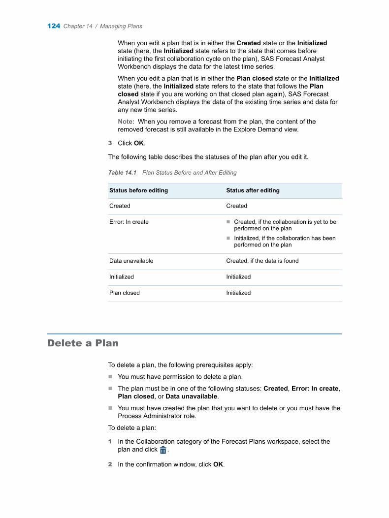
When you edit a plan that is in either the Created state or the Initialized state (here, the Initialized state refers to the state that comes before initiating the first collaboration cycle on the plan), SAS Forecast Analyst Workbench displays the data for the latest time series.
When you edit a plan that is in either the Plan closed state or the Initialized state (here, the Initialized state refers to the state that follows the Plan closed state if you are working on that closed plan again), SAS Forecast Analyst Workbench displays the data of the existing time series and data for any new time series.
Note: When you remove a forecast from the plan, the content of the removed forecast is still available in the Explore Demand view.
3 Click OK.
The following table describes the statuses of the plan after you edit it.
Table 14.1 Plan Status Before and After Editing
Status before editing Status after editing
Created Created
Error: In create n Created, if the collaboration is yet to be performed on the plan
n Initialized, if the collaboration has been performed on the plan
Data unavailable Created, if the data is found
Initialized Initialized
Plan closed Initialized
Delete a Plan
To delete a plan, the following prerequisites apply:
n You must have permission to delete a plan.
n The plan must be in one of the following statuses: Created, Error: In create, Plan closed, or Data unavailable.
n You must have created the plan that you want to delete or you must have the Process Administrator role.
To delete a plan:
1 In the Collaboration category of the Forecast Plans workspace, select the plan and click .
2 In the confirmation window, click OK.
124 Chapter 14 / Managing Plans
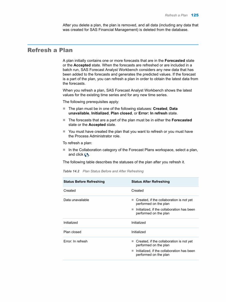
After you delete a plan, the plan is removed, and all data (including any data that was created for SAS Financial Management) is deleted from the database.
Refresh a Plan
A plan initially contains one or more forecasts that are in the Forecasted state or the Accepted state. When the forecasts are refreshed or are included in a batch run, SAS Forecast Analyst Workbench considers any new data that has been added to the forecasts and generates the predicted values. If the forecast is a part of the plan, you can refresh a plan in order to obtain the latest data from the forecasts.
When you refresh a plan, SAS Forecast Analyst Workbench shows the latest values for the existing time series and for any new time series.
The following prerequisites apply:
n The plan must be in one of the following statuses: Created, Data unavailable, Initialized, Plan closed, or Error: In refresh state.
n The forecasts that are a part of the plan must be in either the Forecasted state or the Accepted state.
n You must have created the plan that you want to refresh or you must have the Process Administrator role.
To refresh a plan:
n In the Collaboration category of the Forecast Plans workspace, select a plan, and click .
The following table describes the statuses of the plan after you refresh it.
Table 14.2 Plan Status Before and After Refreshing
Status Before Refreshing Status After Refreshing
Created Created
Data unavailable n Created, if the collaboration is not yet performed on the plan
n Initialized, if the collaboration has been performed on the plan
Initialized Initialized
Plan closed Initialized
Error: In refresh n Created, if the collaboration is not yet performed on the plan
n Initialized, if the collaboration has been performed on the plan
Refresh a Plan 125
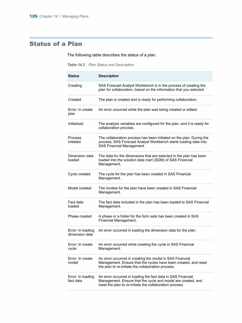
Status of a Plan
The following table describes the status of a plan.
Table 14.3 Plan Status and Description
Status Description
Creating SAS Forecast Analyst Workbench is in the process of creating the plan for collaboration, based on the information that you selected.
Created The plan is created and is ready for performing collaboration.
Error: In create plan
An error occurred while the plan was being created or edited.
Initialized The analysis variables are configured for the plan, and it is ready for collaboration process.
Process initiated
The collaboration process has been initiated on the plan. During the process, SAS Forecast Analyst Workbench starts loading data into SAS Financial Management.
Dimension data loaded
The data for the dimensions that are selected in the plan has been loaded into the solution data mart (SDM) of SAS Financial Management.
Cycle created The cycle for the plan has been created in SAS Financial Management.
Model created The models for the plan have been created in SAS Financial Management.
Fact data loaded
The fact data included in the plan has been loaded to SAS Financial Management.
Phase created A phase or a folder for the form sets has been created in SAS Financial Management.
Error: In loading dimension data
An error occurred in loading the dimension data for the plan.
Error: In create cycle
An error occurred while creating the cycle in SAS Financial Management.
Error: In create model
An error occurred in creating the model in SAS Financial Management. Ensure that the cycles have been created, and reset the plan to re-initiate the collaboration process.
Error: In loading fact data
An error occurred in loading the fact data in SAS Financial Management. Ensure that the cycle and model are created, and reset the plan to re-initiate the collaboration process.
126 Chapter 14 / Managing Plans

Status Description
Error: In create phase
An error occurred in creating the phase. A phase helps you group the form sets. Ensure that the form sets are created properly, and reset the plan to re-initiate the collaboration process.
Template unavailable
The form set has been created, but no data-entry template has been created yet.
Draft created The form set and its data-entry template have been created. The form set can be published at any time.
Publishing form set
SAS Forecast Analyst Workbench is publishing the form sets. The stakeholders receive the form sets and provide inputs for collaboration.
Error: In publishing form set
An error occurred in publishing the form sets. Ensure that the form sets are created properly, and then publish the form sets again.
Open for inputs The forms are available for inputs. Stakeholders can open the forms in Microsoft Excel or in the web-based Form Manager, and provide their inputs.
Consolidating inputs
The forms are open and stakeholders are in the process of providing their inputs.
Error: In import data
An error occurred in importing the data from SAS Financial Management to SAS Forecast Analyst Workbench.
Plan closed The collaboration process is complete. You can now view the collaboration data in the Explore Demand view.
Data unavailable
The data is not available for the specified duration.
Seeding completed
The seeding of the analysis variables is complete.
Error: Seeding failed
An error occurred in seeding the analysis variables.
Deleting SAS Forecast Analyst Workbench is deleting the plan and its relevant information from SAS Forecast Analyst Workbench and SAS Financial Management.
Error: In delete plan
An error occurred while the plan was being deleted. You can manually delete the form sets, models, cycles, and dimension hierarchies that were created for the plan in SAS Financial Management.
Refreshing data SAS Forecast Analyst Workbench is refreshing the data in the selected plan.
Error: In refreshing data
An error occurred in refreshing the plan data.
Status of a Plan 127

128 Chapter 14 / Managing Plans

Part 8Analyzing Forecasts
Chapter 15Exploring Demand . . . . . . . . . . . . . . . . . . . . . . . . . . . . . . . . . . . . . . . . . . . . . . . 131
Chapter 16Performing Scenario Analysis . . . . . . . . . . . . . . . . . . . . . . . . . . . . . . . . . . . . 135
129

130
15
Exploring Demand
Overview of Exploring Demand . . . . . . . . . . . . . . . . . . . . . . . . . . . . . . . . . . . . . . . . . . . . 131
Explore Demand . . . . . . . . . . . . . . . . . . . . . . . . . . . . . . . . . . . . . . . . . . . . . . . . . . . . . . . . . . . 132
Overview of Exploring Demand
Use the Explore Demand view to perform the following tasks:
n drill down and explore historical demand, current demand, future demand, and collaborated demand values
n highlight the demand values that are not within the tolerance limit
The information that you obtain by exploring the demand help you get a better insight into the demand signals. It can also help you understand how the demand is shaped.
For example, suppose your organization manufactures cell phones. As a Territory Manager, you want to view the demand signals for cell phones in your territory. In this scenario, you select product, customer, and location dimensions to explore the demand. You can drill down and view how much demand a customer in your territory is generating for a particular model of cell phone.
The values for a time series in the Explore Demand view might be different from those in the Model Management view. The values are calculated using the analytical procedures in the Model Management view. However, the values in the Explore Demand view are calculated based on mathematical aggregation.
The following guidelines apply to the information that is displayed in the Explore Demand view:
n The view displays the data for the hierarchies that you selected when you created the plan. The data for the hierarchies that are below that aggregation level is not displayed.
n If the plan status is Created, the Explore Demand view shows the actual and predicted values of the forecasts. If the plan status is Plan closed, the Explore Demand view shows the actual, predicted, and collaborated values and the values for any custom-defined analysis variable that was extracted from SAS Financial Management.
n The Explore Demand view does not display the collaboration values for a newly added time period under the following conditions:
o the forecast has been edited and some time series have been removed
131

o the plan status was Plan Closed and it has been refreshed so that the updated values of the forecast appear in the plan
o collaboration is being performed on the plan again
n The Explore Demand view does not display the aggregate values of the start period and end period of the future and historical periods correctly when the periodicity of the forecasts and the periodicity of the plan are different. For example, the periodicity of the forecast is day and the periodicity of the plan is week.
n SAS Forecast Analyst Workbench displays the latest data in the Explore Demand view when you edit the plan in the Created or Initialized state. However, when you edit the plan in any state other than Created or Initialized, the data of the removed time series is also shown in the Explore Demand view.
Explore Demand
To explore demand for a plan, the plan must not be in any in progress state or error state.
1 In the Collaboration category of the Forecast Plans workspace, double-click a plan. The Explore Demand view appears.
2 In the Display Options section of the Configuration Filter pane, specify the following display parameters.
Table 15.1 Fields in the Display Options Section
Field Description
Select analysis variable
Select an analysis variable for which you want to explore demand.
The list of analysis variables depends on the status of the plan and the analysis variables that you selected to extract the data from. If you are exploring the demand for a plan that is in the Created state, only the Actual and Predicted variables are available. If you are exploring the demand for a plan that is in the Plan closed state, the Actual, Predicted, Final, and any custom-defined variables are available.
Allow conditional highlighting
If you select this check box, all the demand values that are not within the tolerance limit are highlighted in red. The demand value that is in bold indicates the demand for the current period.
Compare with
Select the variable from the list with which you want to compare the demand. For example, if you selected Actual in the Select analysis variable list and Predicted in the Compare with list, then you can compare the actual demand values with the predicted demand values.
This list is available only when you select the Allow conditional highlighting check box.
132 Chapter 15 / Exploring Demand

Field Description
Tolerance limit
Enter the tolerance limit (as a percentage) in order to observe variations in your demand shaping with respect to the compared variable. The demand values that are not within the tolerance limit are highlighted in red.
This box is available only when you select the Allow conditional highlighting check box.
Select dimensions
Select the dimensions for which you want to explore demand. The Select dimensions list displays all the dimensions that are present in the plan.
The dimensions that you do not select are used to filter the data and do not appear in the Demand Summary table. For example, if Product, Location, and Customer are the three available dimensions and you select only Product and Location, you can use the third dimension as a filter. You can also choose the order in which the demand should be displayed in the Demand Summary table.
3 In the KPI section of the Configuration Filter pane, specify the following parameters:
a In the Type list, select the type of the key performance indicator.
b In the KPI list, select the key performance indicator.
If you merged forecasts that have different KPIs, you can select the KPI of your choice to explore the demand. For example, if two forecasts with Financial and Operational KPIs are merged to create a plan, you can select the Operational KPI to explore the demand for the plan.
Note: The KPI list shows KPIs of all forecasts that are a part of the plan.
4 In the Time section of the Configuration Filter pane, specify the following display parameters.
Table 15.2 Fields in the Time Section
Field Description
Level Select the hierarchy level of the time dimension on which you want to explore the demand. The Level list displays the hierarchy that you selected when you created the plan. The lowest level available is determined by the aggregation level that you selected when you created the plan. You can select a periodicity in order to explore the demand at that periodicity. For example, select QTR in the Level list to explore the demand for a quarterly period.
Range type Displays the range type.
From Displays the start date of the range. Click and select the start date of the range.
To Displays the end date of the range. Click and select the end date of the range.
Explore Demand 133

5 Select the hierarchy level and one or more of its values. For example, in the Location dimension, you could select the level Country and the value USA in order to explore the demand for USA.
The content and options of the Configuration Filter pane depend on what you selected in the Display Options area. The Configuration Filter pane lists all dimensions and their hierarchies that are selected in the Display Options area in separate sections. For example, if you selected Product, Location, and Customer dimensions in the Displays Options area, the Configuration Filter pane lists three separate components for each dimension.
Note: You can select multiple values of the selected level for a dimension if you have not selected the dimension in the Select dimensions list in the Display Options section.
6 Click Apply. The demand for the analysis variables that you selected is displayed. You can click Reset to reset the options.
7 In the Demand Summary table, view the demand for the dimensions and time that you select. The Demand Summary table displays the current value of the demand in bold and the demand values that are not within the selected tolerance limit in red.
Drill down or filter the demand in the hierarchy by clicking different values for the dimensions. As you click different values, the Demand Summary table displays the respective demand values. You can use the link to drill down into a dimension member and explore the demand for its descendents.
8 Click the Summary tab to view the demand values for the row that you selected in the Demand Summary table. The Summary tab enables you to compare the demand values for all the analysis variables that are included in the plan.
9 Click the Drill Path tab to view the navigation path of the demand exploration. The navigation path contains the dimension nodes that you selected while you were exploring the demand. You can click a row to go back to a previous step on the Drill Path tab.
134 Chapter 15 / Exploring Demand

16
Performing Scenario Analysis
Workflow for Scenario Analysis . . . . . . . . . . . . . . . . . . . . . . . . . . . . . . . . . . . . . . . . . . . 135
Create a Scenario . . . . . . . . . . . . . . . . . . . . . . . . . . . . . . . . . . . . . . . . . . . . . . . . . . . . . . . . . 136
Edit the Values of Independent Variables . . . . . . . . . . . . . . . . . . . . . . . . . . . . . . . . . . 136About Editing Independent Variables . . . . . . . . . . . . . . . . . . . . . . . . . . . . . . . . . . . . . . 136Edit a Value in the Input Table . . . . . . . . . . . . . . . . . . . . . . . . . . . . . . . . . . . . . . . . . . . . 137Edit Values By Using the Input Calculator . . . . . . . . . . . . . . . . . . . . . . . . . . . . . . . . . 137
Run and Save a Scenario . . . . . . . . . . . . . . . . . . . . . . . . . . . . . . . . . . . . . . . . . . . . . . . . . . 138
Reset a Scenario . . . . . . . . . . . . . . . . . . . . . . . . . . . . . . . . . . . . . . . . . . . . . . . . . . . . . . . . . . 139
Delete a Scenario . . . . . . . . . . . . . . . . . . . . . . . . . . . . . . . . . . . . . . . . . . . . . . . . . . . . . . . . . . 139
Export Scenario Values . . . . . . . . . . . . . . . . . . . . . . . . . . . . . . . . . . . . . . . . . . . . . . . . . . . . 139
Workflow for Scenario Analysis
Using scenario analysis, you can shape demand by varying the future values of the factors that influence the demand. The factors that influence the demand can be internal or external and can include price, advertising, sales promotions, marketing events, economic factors, and other factors.
For example, you can use scenario analysis to determine what happens to the demand for gasoline when the price of gasoline increases by 5%.
The workflow for performing a scenario analysis consists of the following tasks:
1 Create a scenario.
You must create the scenario when you are performing the scenario analysis for the first time for the selected time series. After you create the scenario and save it, you do not need to re-create it for analyzing different scenarios until the model of the time series changes.
2 Edit the values of independent variables.
The factors that influence demand can be internal or external, and can include price, advertising, sales promotions, marketing events, economic factors, and other factors. By varying the values of these factors, you can determine their effects on demand. For example, you can determine what happens to the demand for gasoline when the price of gasoline increases by 5%.
135

3 Run and save the scenario. Before you save the scenario, you can view the scenario values in graphical form. In the graphs, you can also see a comparison of the predicated demand values and scenario demand values.
4 (Optional) Export scenario values.
Create a Scenario
The following prerequisites apply when you create a scenario:
n The forecast must be in the Forecasted state.
n The model that is applied to the time series must contain at least one independent variable.
n You must be creating the scenario for this time series for the first time. If you attempted to create a scenario for the selected time series but you did not save it, you can create it again.
To create a scenario:
1 Double-click a forecast in the Forecasts category of the Forecast Plans workspace. The Model Management view appears.
2 (Optional) On the Table View tab of the Model Management view, filter the time series that have independent variables.
For more information about filtering the time series, see “Filter the Time Series” on page 63.
3 Select the time series for which you want to perform the scenario analysis, and click the Scenario tab. (You can select only one time series at a time.) The Scenario tab displays the list of independent variables that are used in the model for the selected time series, scenario demand, and predicted demand. The scenario demand is the same as that of the forecasted demand before you run the scenario for the first time. If you have saved the scenario before, then the saved scenario demand values are displayed.
4 On the Scenario tab of the Model Management view, click . The Scenario tab displays the values of the independent variables that are used in the model to calculate the scenario demand.
Note: The button is available only if you are creating the scenario for the selected time series for the first time or if you did not save the scenario.
Note: By default, the predicted demand and the scenario demand are same.
Edit the Values of Independent Variables
About Editing Independent Variables
You can edit the future values of the independent variables in the following ways:
136 Chapter 16 / Performing Scenario Analysis

n by typing one or more values in the input table.
For example, to run a scenario for the holiday season, you might want to increase the cost of transport charges for December.
n by using the input calculator. You can use this method when you want to specify all new values in the input table.
For example, if you are running a scenario for a weather forecast report, you might want to decrease the value of rainfall by 8% for the entire year.
You can edit the values of the independent variables and then run the scenario. If the result of the scenario is not satisfactory, you can edit the values of the independent variables again.
Edit a Value in the Input Table
To edit the future value of an input variable in the input table:
1 In the input table of the Scenarios tab of the Model Management view, double-click a cell for the time period that you want to override.
2 Type the new value and press Enter.
3 Run the scenario. For more information about running the scenario, see “Run and Save a Scenario” on page 138.
Edit Values By Using the Input Calculator
To edit the values for multiple time periods:
1 Select the input variable whose values you want to change in the input table.
2 Click . The Input Calculator window appears.
3 Enter the appropriate information for the following parameters.
Table 16.1 Parameters in the Input Calculator Window
Parameter Description
Adjustment Select this option, click + or –, and then enter the adjustment value, as a percentage.
For example, click +, and then type 10. The application adds 10% to the values in all the time periods for the selected independent variable.
Set to value Select this option to assign a value to each time period.
Edit the Values of Independent Variables 137

Parameter Description
Distribution method
Select the appropriate option to distribute the value that you entered in the Set to value field. You can select one of the following options:n Assign value to each period: Select this option to assign the
value that you entered to each time period of the selected independent variable.
n Split evenly: Select this option to split the value evenly across all time periods of the selected independent variable.
n Split proportional to current input value: Select this option to split the value proportionately to the current value of all time periods.
Note: The options in this list are available only when you select the Set to value option.
4 Click OK.
5 (Optional) Click to reset the values of the independent variables.
6 Run the scenario. For more information about running the scenario, see “Run and Save a Scenario” on page 138.
Run and Save a Scenario
You must run the scenario in order to obtain the scenario demand and compare it with the predicted demand. You can run the scenario when you have edited the values of the independent variables for the selected time series. You can run the scenario when the status of the forecast is Forecasted.
To run and save a scenario:
1 On the Scenario tab of the Model Management view, edit the values of the independent variables, and click .
By default, the predicted demand and the scenario demand are same. After you run the scenario analysis, the Scenario tab updates the scenario, so these values might change. You can change the values of independent variables to generate different scenarios.
2 (Optional) Change the time series.
3 (Optional) Click to view the scenario values in graphical form. The Scenario Demand Line Chart window displays the predicted demand and scenario demand in graphical form.
4 If you are satisfied with the results of a scenario, click . The latest values of the scenario are saved for future use.
Note: If a scenario already exists for a time series and the model for the time series has changed, then delete the scenario and re-create it to obtain the latest scenario values based on the new model.
138 Chapter 16 / Performing Scenario Analysis

5 (Optional) Export the values of the scenario. For more information about exporting the scenario values, see “Export Scenario Values” on page 139.
6 (Optional) To use the scenario values in a forecast, accept the forecast. After you accept the forecast, SAS Forecast Analyst Workbench uses the scenario values for the time series instead of using the predicted values. After you accept the forecast, you might want to reconcile the forecast.
Reset a Scenario
Reset the scenario to retain the original values of the independent variables. When you reset the scenario, SAS Forecast Analyst Workbench retains the values of the independent variables that were used when you saved the scenario. You can reset the scenario at any time during the process of analyzing various value of independent variables.
To reset the scenario:
n On the Scenario tab of the Model Management view, click .
Note: The button is available when you have edited the values of the input parameters.
Delete a Scenario
Delete the scenario to start the scenario analysis from the beginning. When you delete a scenario, the altered values of independent variables are reset to the loaded values.
To delete a scenario:
1 On the Scenario tab of the Model Management view, click .
2 In the confirmation window, click Yes.
Export Scenario Values
When you perform a scenario analysis, the values that you change do not change the predicted values. You can export the values of all independent variables, predicted demand values, and scenario demand values to a .csv file.
To export the scenario values:
1 Click . The Export Scenario Values window appears.
2 Navigate to the location where you want to save the file.
3 Enter a name for the file, and click Save.
Export Scenario Values 139

The values of all independent variables, predicted demand values, and scenario demand values are exported to a .csv file.
140 Chapter 16 / Performing Scenario Analysis

Part 9Administering Product Life Cycle in SAS Forecast Analyst Workbench
Chapter 17Managing the Life Cycle of Products . . . . . . . . . . . . . . . . . . . . . . . . . . . . . . . 143
141

142
17
Managing the Life Cycle of Products
Product Life Cycle Workflow . . . . . . . . . . . . . . . . . . . . . . . . . . . . . . . . . . . . . . . . . . . . . . . 143
Search for Products . . . . . . . . . . . . . . . . . . . . . . . . . . . . . . . . . . . . . . . . . . . . . . . . . . . . . . . 144
Specify Phase-in Details for a Product . . . . . . . . . . . . . . . . . . . . . . . . . . . . . . . . . . . . . 145
Specify Phase-out Details for a Product . . . . . . . . . . . . . . . . . . . . . . . . . . . . . . . . . . . 146
Define a Successor Product . . . . . . . . . . . . . . . . . . . . . . . . . . . . . . . . . . . . . . . . . . . . . . . 148
Manage the Life Cycle for Multiple Products Simultaneously . . . . . . . . . . . . . . . 150
Generate Forecast Values for New Relationships . . . . . . . . . . . . . . . . . . . . . . . . . . 151
Managing Life Cycle Details for a Product . . . . . . . . . . . . . . . . . . . . . . . . . . . . . . . . . 152Managing Phase-in Details . . . . . . . . . . . . . . . . . . . . . . . . . . . . . . . . . . . . . . . . . . . . . . . 152Managing Phase-out Details . . . . . . . . . . . . . . . . . . . . . . . . . . . . . . . . . . . . . . . . . . . . . 153Managing Successor Product Details . . . . . . . . . . . . . . . . . . . . . . . . . . . . . . . . . . . . . 154
Product Life Cycle Workflow
SAS Forecast Analyst Workbench enables you to manage a suite of products and their life cycle information. SAS Forecast Analyst Workbench uses the life cycle information to forecast the demand for the products. Planners and forecast analysts can view the information about products in the Model Management view and in the Explore Demand view.
SAS Forecast Analyst Workbench uses the following systematic workflow for managing the product life cycle.
1 Select a product that you want to manage. You can search for a product from the list of products that belong to you.
For more information about searching a product, see “Search for Products” on page 144
2 Specify phase-in details for the product.
Define the phase-in date or introduction date of the product with respect to non-product dimensions. For example, product A is introduced in Germany on September 01. You can define multiple phase-in dates for the product. For example, product A is introduced in Germany on September 01, but in Japan, it is introduced on September 15. Also define relationships for the product.
143

The phase-in date is the date on which the first customer transaction for the product will happen. Prior to this date, the product does not have any demand.
For more information about defining phase-in details for a product, see “Specify Phase-in Details for a Product” on page 145.
3 Specify phase-out details for the product. Also define relationships for the product. You can define multiple different phase-out dates for different relationships. A phase-out date can be permanent or temporary.
The phase-out date is the date on which the last customer transaction for the product will take place. After this date, no actual demand for this product would be considered for shipments planning.
For more information about defining phase-out details for a product, see “Specify Phase-out Details for a Product” on page 146.
4 Define a successor product for the product that is phasing out. The successor is the product that replaces the original product. After successor is phased in, the actual demand of the successor would be considered for shipments planning.
At least one successor product must be defined in order to define the successor relationships.
For more information about defining successors, see “Define a Successor Product” on page 148.
5 Generate forecast values for newly phased in relationships in order to use them in the forecast.
For more information about generating forecast values, see “Generate Forecast Values for New Relationships” on page 151.
Search for Products
Find that product that you want to work on. You can search for products by name or by specifying search criteria.
You must have permission to search the products.
To search for products:
1 In the Administration workspace, click Products. The Products category appears.
The Products category appears by default since it is the only category in the Administration workspace.
2 In the Products category, click Search. The Search window appears.
3 Enter the search criteria.
Enter the name of the product in the Enter product name field, or expand the dimensions and select the search criteria. For example, expand Select Customers, and then select the customers that are selling the product. You can use this approach when the product has been already introduced or phased-in at the customer.
144 Chapter 17 / Managing the Life Cycle of Products

4 Click Search.
SAS Forecast Analyst Workbench displays the products that satisfy the search criteria. If the search result contains more than 1000 products, you must re-enter the search criteria to refine your search. If you do not refine the search criteria, SAS Forecast Analyst Workbench displays the first 1000 products.
Specify Phase-in Details for a Product
As part of the life cycle plan for a product, you must define a phase-in date for it. You must also specify relationships for the product or the applicability of the product. For example, Product A is not sold in all countries in the EMEA region. However, it is going to be sold in Canada. For each phase-in date, you must specify one or more relationships to the non-product dimensions. The combination of a product and a relationship can be phased-in only once. You must have permission to add a phase-in relationship.
To specify phase-in details:
1 In the Products category of the Administration workspace, double-click a product. The Product Life Cycle view appears with three sections: Phase-in Details, Phase-out Details, and Successor Details.
2 In the Phase-in Details section, click . The Add Phase-in Details window appears.
3 In the Add Phase-in Details window, enter appropriate information in the following fields.
Table 17.1 Fields on the Add Phase-in Details Window
Field Description
Phase-in date Select a date to phase in or introduce the product.
Phase-in Relationships
This section contains various tabs enabling you to select values for each dimension. By selecting values for each dimension, a phase-in relationship is added. You can add a phase-in relationship either by selecting suggested values for each dimension or by selecting new values for each dimension.
The suggested values are shown for existing relationships. If no relationship is set up, no suggested values are available.
While defining relationships, you can select multiple members simultaneously for one dimension. When you do so, the selection for the other dimensions is limited to one member.
Note: Based on the settings that the administrator has defined, you might not see all dimensions while adding a relationship. However, you can view all dimensions while viewing a relationship.
4 Click Save. The Edit Phase-in Details window appears and displays the phase-in date and relationships.
Specify Phase-in Details for a Product 145
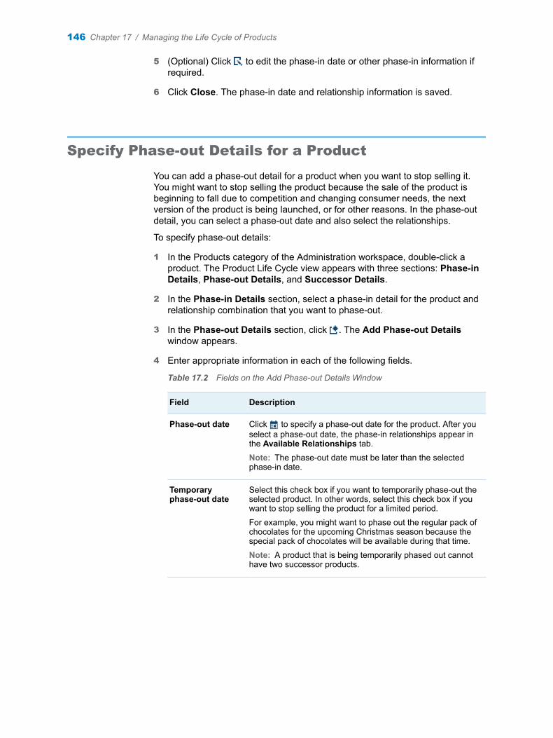
5 (Optional) Click to edit the phase-in date or other phase-in information if required.
6 Click Close. The phase-in date and relationship information is saved.
Specify Phase-out Details for a Product
You can add a phase-out detail for a product when you want to stop selling it. You might want to stop selling the product because the sale of the product is beginning to fall due to competition and changing consumer needs, the next version of the product is being launched, or for other reasons. In the phase-out detail, you can select a phase-out date and also select the relationships.
To specify phase-out details:
1 In the Products category of the Administration workspace, double-click a product. The Product Life Cycle view appears with three sections: Phase-in Details, Phase-out Details, and Successor Details.
2 In the Phase-in Details section, select a phase-in detail for the product and relationship combination that you want to phase-out.
3 In the Phase-out Details section, click . The Add Phase-out Details window appears.
4 Enter appropriate information in each of the following fields.
Table 17.2 Fields on the Add Phase-out Details Window
Field Description
Phase-out date Click to specify a phase-out date for the product. After you select a phase-out date, the phase-in relationships appear in the Available Relationships tab.
Note: The phase-out date must be later than the selected phase-in date.
Temporary phase-out date
Select this check box if you want to temporarily phase-out the selected product. In other words, select this check box if you want to stop selling the product for a limited period.
For example, you might want to phase out the regular pack of chocolates for the upcoming Christmas season because the special pack of chocolates will be available during that time.
Note: A product that is being temporarily phased out cannot have two successor products.
146 Chapter 17 / Managing the Life Cycle of Products
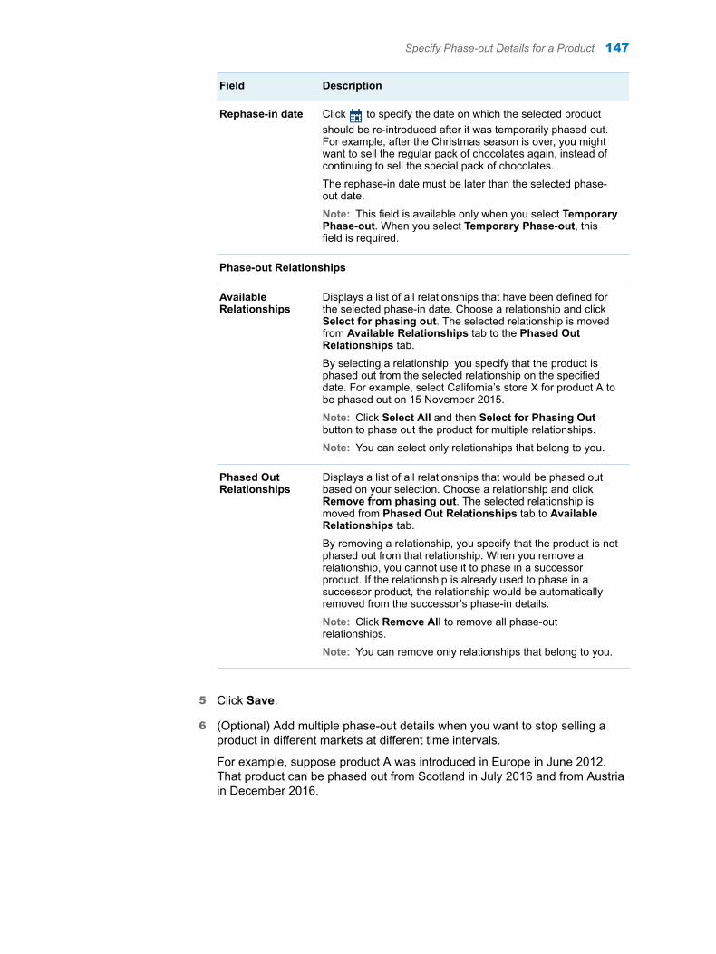
Field Description
Rephase-in date Click to specify the date on which the selected product should be re-introduced after it was temporarily phased out. For example, after the Christmas season is over, you might want to sell the regular pack of chocolates again, instead of continuing to sell the special pack of chocolates.
The rephase-in date must be later than the selected phase-out date.
Note: This field is available only when you select Temporary Phase-out. When you select Temporary Phase-out, this field is required.
Phase-out Relationships
Available Relationships
Displays a list of all relationships that have been defined for the selected phase-in date. Choose a relationship and click Select for phasing out. The selected relationship is moved from Available Relationships tab to the Phased Out Relationships tab.
By selecting a relationship, you specify that the product is phased out from the selected relationship on the specified date. For example, select California’s store X for product A to be phased out on 15 November 2015.
Note: Click Select All and then Select for Phasing Out button to phase out the product for multiple relationships.
Note: You can select only relationships that belong to you.
Phased Out Relationships
Displays a list of all relationships that would be phased out based on your selection. Choose a relationship and click Remove from phasing out. The selected relationship is moved from Phased Out Relationships tab to Available Relationships tab.
By removing a relationship, you specify that the product is not phased out from that relationship. When you remove a relationship, you cannot use it to phase in a successor product. If the relationship is already used to phase in a successor product, the relationship would be automatically removed from the successor’s phase-in details.
Note: Click Remove All to remove all phase-out relationships.
Note: You can remove only relationships that belong to you.
5 Click Save.
6 (Optional) Add multiple phase-out details when you want to stop selling a product in different markets at different time intervals.
For example, suppose product A was introduced in Europe in June 2012. That product can be phased out from Scotland in July 2016 and from Austria in December 2016.
Specify Phase-out Details for a Product 147

Define a Successor Product
The following guidelines apply to defining a successor product:
n A successor product cannot have two predecessor products that contain temporary phase-out dates.
n A phased-out relationship must be defined for the product before you define a successor product.
To specify a successor product:
1 In the Products category of the Administration workspace, double-click a product. The Product Life Cycle view appears with three sections: Phase-in Details, Phase-out Details, and Successor Details.
2 In the Phase-in Details section, select a phase-in detail. The Phase-out Details section displays the phase-out details that are associated with the selected phase-in detail.
3 In the Phase-out Details section, select a phase-out detail. The Successor Details section displays the successor details that are associated with the selected phase-out detail.
4 In the Successor Details section, click . The Define Successor Details window displays a list of all successors that are available for the selected product.
5 Enter the appropriate information in each field. The following table describes each field.
Table 17.3 Fields in the Define Successor Details Window
Field Description
Successor’s phase-in date
Specify a date that can be used as the successor’s phase-in date.
The phase-in date of the successor product must be later than the phase-out date of the original product. For example, suppose the phase-out date for product A is 01 November 2014. The phase-in date of product B (which is a successor for product A) must be later than 01 November 2014.
Note: After the successor’s phase-in date, SAS Forecast Analyst Workbench uses the demand of the predecessor for the specified relationships to generate the successor's forecast for the specified relationships. The phase-in date of the successor product must immediately follow the phase-out date of the predecessor product. The rephase-in date of the predecessor product should immediately follow the phase-out date of the successor product.
148 Chapter 17 / Managing the Life Cycle of Products

Field Description
Successor Products
Displays a list of all products that can act as a successor for the selected product. Select a product and then click to use it as a successor.
In order to view the successor and predecessor products chaining information in the Changed Time Series tab of the Model Management view, ensure that the successor and predecessor products are included in the forecast.
Note: A product cannot act as its own successor. For example, product A cannot be its own successor product.
Available Relationships
Displays a list of relationships that are available for phasing in the successor. All the listed relationships are phased-out for the predecessor product. Select a relationship and click Select for phase-in. The selected relationship is moved from the Available Relationships tab to Successor’s Phased In Relationships tab.
You can select multiple products as successors. When you select multiple products as successors, the Available Relationships tab displays the common relationships that are available to the selected successor products.
Note: The relationships that you see on the Available Relationships tab depend on the relationships that are defined for the selected phase-out date in the Phase-out Details section.
Successor’s Phased In Relationships
Displays a list of relationships that you selected for phasing in the successor product. Select relationships and click Deselect from phase-in link to remove the relationships from phasing in the successor.
6 Click Save.
7 Define the scale factor for the successor product. With the scale factor, you can scale up or scale down the demand of the relationship for the successor product. SAS Forecast Analyst Workbench scales the successor’s demand (that is based on the historical demand of the predecessor product at the selected relationship) up or down by the specified scale factor.
a In the Successor Details section, click the Number of Relationships link for the product for which you want to define the scale factor. The Successor Details window appears.
b Select a relationship, and click Scale Factor. The Edit Scale Factor window appears.
c Enter the scale factor. For example, if you enter 2 for successor product A at store X in Indiana, SAS Forecast Analyst Workbench multiplies the demand for product A at store X in Indiana by 2.
d Click Save.
SAS Forecast Analyst Workbench scales the demand for the successor product up or down with the number that you entered.
TIP You can open the Product Life Cycle view for the successor product and notice that the phase-in date entered in the predecessor’s Successor Details
Define a Successor Product 149

pane is listed in the successor’s Phase-in Details pane. Select the phase-in date and define a phase-out date for all the relationships for which the predecessor will be re-introduced. Furthermore, define the phase-out date of the successor product as a date that is earlier than the rephase-in date of the predecessor product. For example, suppose product A is phasing out on May 31 and is being rephased in on September 01. Product B is the successor for product A. In this case, product B must be phased in after May 31 and be phased out before September 01.
Manage the Life Cycle for Multiple Products Simultaneously
1 In the Products category of the Administration workspace, select multiple products by pressing and holding the Ctrl key, and click . The Product Life Cycle view displays a list of all selected products.
2 In the Product Life Cycle view, you can perform the following actions:
n Add a phase-in date, and then define phase-in relationships.
1 Click , and then select Add Phase-in Details. The Add Phase-in Details window appears.
2 Select a phase-in date, and then define relationships.
For more information about the fields in the Add Phase-in Details window, see Table 17.1 on page 145.
n Edit the phase-in relationships.
1 Click , and then select Modify Phase-in Relationships. The Edit Phase-in Details window appears.
2 Enter the appropriate information in the Edit Phase-in Details window, and click Save.
For more information about the Edit Phase-in Details window, see Table 17.4 on page 152.
n Add a phase-out date, and then define phase-out relationships.
1 Click , and then select Add Phase-out Details. The Add Phase-out Details window appears.
2 Enter the appropriate information.
For more information about fields in the Add Phase-out Details window, see Table 17.2 on page 146.
n Edit the phase-out relationships.
To edit the phase-out relationships, perform the following steps:
1 Click , and then select Modify Phase-out Relationships. The Edit Phase-out Details window appears.
2 Enter the appropriate information.
150 Chapter 17 / Managing the Life Cycle of Products

For more information about the Edit Phase-out Details window, see Table 17.2 on page 146.
n Add a successor phase-in date, and then define successor relationships.
1 Click and then select Add Successor Details. The Define Successor Details window appears.
2 Enter the appropriate information and click Save.
For more information about the Define Successor Details window, see Table 17.3 on page 148.
n Edit the successor details.
1 Click , and then select Modify Successor Phase-in Relationships. The Edit Successor Details window appears.
2 Enter the appropriate information.
Edit the scale factor by clicking the number in the Successor Details column.
For more information about the Edit Successor Details window, see Table 17.3 on page 148.
Generate Forecast Values for New Relationships
SAS Forecast Analyst Workbench generates the forecasted values automatically for the newly phased in relationships. The forecasted values are generated based on the time series for similar relationships. For example, suppose you defined that the product Projector X350UV will be introduced in Los Angeles on 01 June 2016. In this case, SAS Forecast Analyst Workbench automatically generates the forecast for Projector X350UV in Los Angeles for June 2016.
When the new set of periodical data becomes available and is loaded to SAS Forecast Analyst Workbench, SAS Forecast Analyst Workbench generates the predicted demand for newly phased in relationships automatically. This predicted demand of the newly phased in relationships becomes available to the forecast if the new phased-in relationships are a part of the forecast
To generate forecast values for new relationships, in the Products category of the Administration workspace, click .
SAS Forecast Analyst Workbench generates the forecasted values for all newly phased in relationships for all products.
Generate Forecast Values for New Relationships 151

Managing Life Cycle Details for a Product
Managing Phase-in Details
Edit a Phase-in Detail
As your business requirements change, you might need to edit the phase-in date. Or, you might want to add relationships or delete relationships that are associated with the phase-in date.
To edit phase-in details:
1 In the Products category of the Administration workspace, double-click a product. The Product Life Cycle view appears with three sections: Phase-in Details, Phase-out Details, and Successor Details.
2 In the Phase-in Details section, click . The Edit Phase-in Details window appears.
3 In the Edit Phase-in Details window, enter the appropriate information.
Table 17.4 Fields on the Edit Phase-in Details Window
Field Description
Phase-in date Displays a phase-in date.
Edit Displays the phase-in date. Click Edit button to edit the phase-in date. After you click this button, the button becomes available and then you can choose a different phase-in date. Click , select a phase-in date, and then click Save.
Phase-in relationships
Displays the phase-in relationships of the product.
Click to add phase-in relationships. When you click this button, the Add Phase-in Details window appears and enables you to add phase-in relationships.
Click to delete the selected phase-in relationship.
When you delete a phased in relationship, all phase-in relationships that do not have phase-out details and successor details are deleted. Deleting a phase-in relationship is different from phasing out a relationship. When you delete a phase-in relationship, it will no longer be available for phase-out and succession. A phase-out relationship discontinues the product for that relationship (for example, a particular combination of facility and customer).
4 Click Save.
152 Chapter 17 / Managing the Life Cycle of Products

Delete a Phase-in Detail
You can delete phase-in details when they are not required. When you delete phase-in details, all the phase-out and successor details associated with the phase-in details are also deleted.
To delete a phase-in detail:
1 In the Products category of the Administration workspace, double-click a product. The Product Life Cycle view appears with three sections: Phase-in Details, Phase-out Details, and Successor Details.
2 In the Phase-in Details section, select a phase-in detail and click .
3 In the confirmation window, click OK.
Managing Phase-out Details
Edit a Phase-out Detail
As your business requirements change, you might need to edit the phase-out details of a product. You can edit the phase-out date and relationships for a product. You can also edit the rephase-in date. You must have permission to edit a phase-out detail.
To edit phase-out details:
1 In the Products category of the Administration workspace, double-click a product. The Product Life Cycle view appears with three sections: Phase-in Details, Phase-out Details, and Successor Details.
2 In the Phase-in Details section, select a phase-in detail. The Phase-out Details section displays all phase-out details that are defined for the selected phase-in detail.
3 In the Phase-out Details section, select a phase-out detail, and click . The Edit Phase-out Details window appears.
4 Edit the phase-out details.
For more information about the fields of the Edit Phase-out Details window, see Table 17.2 on page 146.
5 Click Save.
Delete a Phase-out Detail
Delete a phase-out detail if you no longer want to phase out the product on that particular date and at those relationships. After you delete a phase-out detail, all relationships and all successor products associated with the phase-out date are deleted. You must have permission to delete a phase-out detail.
To delete a phase-out detail:
1 In the Product category of the Administration workspace, double-click a product. The Product Life Cycle view appears with three sections: Phase-in Details, Phase-out Details, and Successor Details.
Managing Life Cycle Details for a Product 153

2 In the Phase-in Details section, select a phase-in detail. The Phase-out Details section displays all the phase-out details that are associated with the selected phase-in detail.
3 Select a phase-out detail and click .
4 In the confirmation window, click OK.
Managing Successor Product Details
Edit Successor Details
Edit the detail of a successor when the business requirement changes. You can edit only the successor relationships.
To edit a successor detail:
1 In the Products category of the Administration workspace, double-click a product. The Product Life Cycle view appears with three sections: Phase-in Details, Phase-out Details, and Successor Details.
2 In the Phase-in Details section, select a phase-in detail. The Phase-out Details section displays the phase-out details that are associated with the selected phase-in detail.
3 In the Phase-out Details section, select a phase-out detail. The Successor Details section displays the successor details that are associated with the selected phase-out detail.
4 In the Successor Details section, select a successor detail, and click . The Define Successor Details window displays a list of all the relationships that have been phased in with the successor product.
5 Edit the successor details.
You can remove relationships from the Successor's Phased-In Relationships tab by selecting them and clicking Deselect from phase-in button. You can add relationships to the Successor's Phased-In Relationships tab by selecting them on the Available Relationships tab and clicking Select for phase-in button.
For more information about the Define Successor Detail window, see Table 17.3 on page 148.
Note: You cannot edit the phase-in date and also cannot change the successor product.
6 Click Save.
Delete Successor Details
1 In the Products category of the Administration workspace, double-click a product. The Product Life Cycle view appears with three sections: Phase-in Details, Phase-out Details, and Successor Details.
2 In the Phase-in Details section, select a phase-in detail. The Phase-out Details section displays a list of all phase-out details that are associated with the selected phase-in detail.
154 Chapter 17 / Managing the Life Cycle of Products

3 In the Phase-out Details section, select a phase-out detail. The Successor Details section displays a list of all successor products that are associated with the selected phase-out detail.
4 In the Successor Details section, select a successor detail and click .
5 In the confirmation window, click OK.
Managing Life Cycle Details for a Product 155

156 Chapter 17 / Managing the Life Cycle of Products

Part 10Generating Reports
Chapter 18Working with Reports . . . . . . . . . . . . . . . . . . . . . . . . . . . . . . . . . . . . . . . . . . . . 159
157

158

18
Working with Reports
About Reports . . . . . . . . . . . . . . . . . . . . . . . . . . . . . . . . . . . . . . . . . . . . . . . . . . . . . . . . . . . . . 159
View a Report . . . . . . . . . . . . . . . . . . . . . . . . . . . . . . . . . . . . . . . . . . . . . . . . . . . . . . . . . . . . . 159
Create a Report . . . . . . . . . . . . . . . . . . . . . . . . . . . . . . . . . . . . . . . . . . . . . . . . . . . . . . . . . . . . 160
About Reports
Reports and analysis form the backbone of any business. With SAS Forecast Analyst Workbench, you can generate reports to analyze business information. SAS Forecast Analyst Workbench is tightly integrated with SAS Web Report Studio and SAS Visual Analytics for performing report-related tasks.
In the Reports workspace, you can perform the following tasks:
n view a report
n launch SAS Web Report Studio or SAS Visual Analytics Reporting to create a report
n search for a report
n refresh reports
View a Report
You can view a report that was created in SAS Visual Analytics in SAS Visual Analytics Viewer. You can view a report that was created in SAS Web Report Studio in that application.
You can edit a report in SAS Visual Analytics if you have the required permission.
To view a report:
n In the Reports workspace, double-click a report. Alternatively, select a report, and click Open.
159

Create a Report
You can create a report in order to understand and analyze business information. You must have permission to create a report.
To create a report:
1 In the Reports workspace, click , and then select one of the following options:
n Create Report in SAS Web Report Studio
n Create Report in SAS Visual Analytics
Depending on the option that you select, SAS Web Report Studio or SAS Visual Analytics Designer opens in a new tab in the browser.
2 Specify the report criteria and click OK.
For more information about SAS Web Report Studio, see SAS Web Report Studio: User’s Guide.
For more information about SAS Visual Analytics, see SAS Visual Analytics: User’s Guide.
160 Chapter 18 / Working with Reports

Part 11Appendix
Appendix 1Performing Multi-Tier Causal Analysis . . . . . . . . . . . . . . . . . . . . . . . . . . . . . 163
161

162

Appendix 1Performing Multi-Tier Causal Analysis
About Multi-Tiered Causal Analysis . . . . . . . . . . . . . . . . . . . . . . . . . . . . . . . . . . . . . . . . 163
Perform Multi-Tiered Causal Analysis . . . . . . . . . . . . . . . . . . . . . . . . . . . . . . . . . . . . . . 163
About Multi-Tiered Causal Analysis
Multi-tiered causal analysis links a series of quantitative methods together in order to measure the impact of sales and marketing strategies on consumer demand. Then, using the coefficients of the demand model, the analysis executes various what-if scenarios to shape and predict the demand. Finally, demand and supply are linked by using analytics rather than by using just judgment.
In other words, you can forecast the future values of an independent variable and use those values to predict the demand for your products.
Perform Multi-Tiered Causal Analysis
When you perform multi-tiered causal analysis, the following prerequisites apply:
n You must identify the independent variable when you are deploying SAS Forecast Analyst Workbench.
n The planner and the administrator must be familiar with the forecasts and plans.
n The status of the plan must be either Created, Initialized, or Plan closed.
To perform multi-tiered causal analysis:
1 If you are an administrator, complete the following steps:
a Open the table INDEP_VAR_TABLE that is in the CONFIG library. This table is available after you run the faw_0001_generate_config_datamart job. Then select the independent variable that you want to use.
b Run the faw_0002_populate_config_tables job in order to create the KPI_CONFIG table.
163

For more information, see SAS Forecast Analyst Workbench: Administrator’s Guide.
c In the KPI_CONFIG table, add the independent variable as a KPI and enter the other required information.
The two KPIs set up for multi-tiered causal analysis process must use the same dimensions.
d Run the remaining ETL jobs.
2 If you are a planner, complete the following steps:
a Create a forecast for the independent variable that you added as a KPI.
For more information about creating a forecast, see Chapter 3, “Creating a Forecast,” on page 13.
You can use other independent variables as causal variables to forecast the values of the selected independent variable.
Note: The forecast must include all the dimensions of the KPI.
TIP Select all the dimensions in the forecast in order to import the data from SAS Financial Management.
b Run the forecast, predict the future values of the independent variables, and accept the forecast.
c Create a plan in order to write back the predicted values of the independent variable. While you are creating the plan, select the forecast that you just created for performing multi-tiered causal analysis.
For more information about creating a plan, see “Create a Plan” on page 113.
Note: When you create the plan, select the lowest hierarchy level as the aggregation level for each dimension.
d (Optional) Perform collaboration on the plan.
You can choose to perform collaboration planning on the plan in order to solicit the opinions of various stakeholders regarding the predicted values of the independent variable. After you have received the inputs from all stakeholders, complete the collaboration. The plan status becomes Plan closed.
3 If you are an administrator, complete the following steps:
a Open the following job in the workspace of SAS Data Integration Studio:
/Products/SAS Forecast Analyst Workbench/5.3 Jobs/Wave08 (Utilities)/faw_0805_mtca_writeback
b Right-click in the empty area of the workspace, and click Properties. The Properties window appears.
c Click the Precode and Postcode tab, and specify the following parameters:
164 Appendix 1 / Performing Multi-Tier Causal Analysis
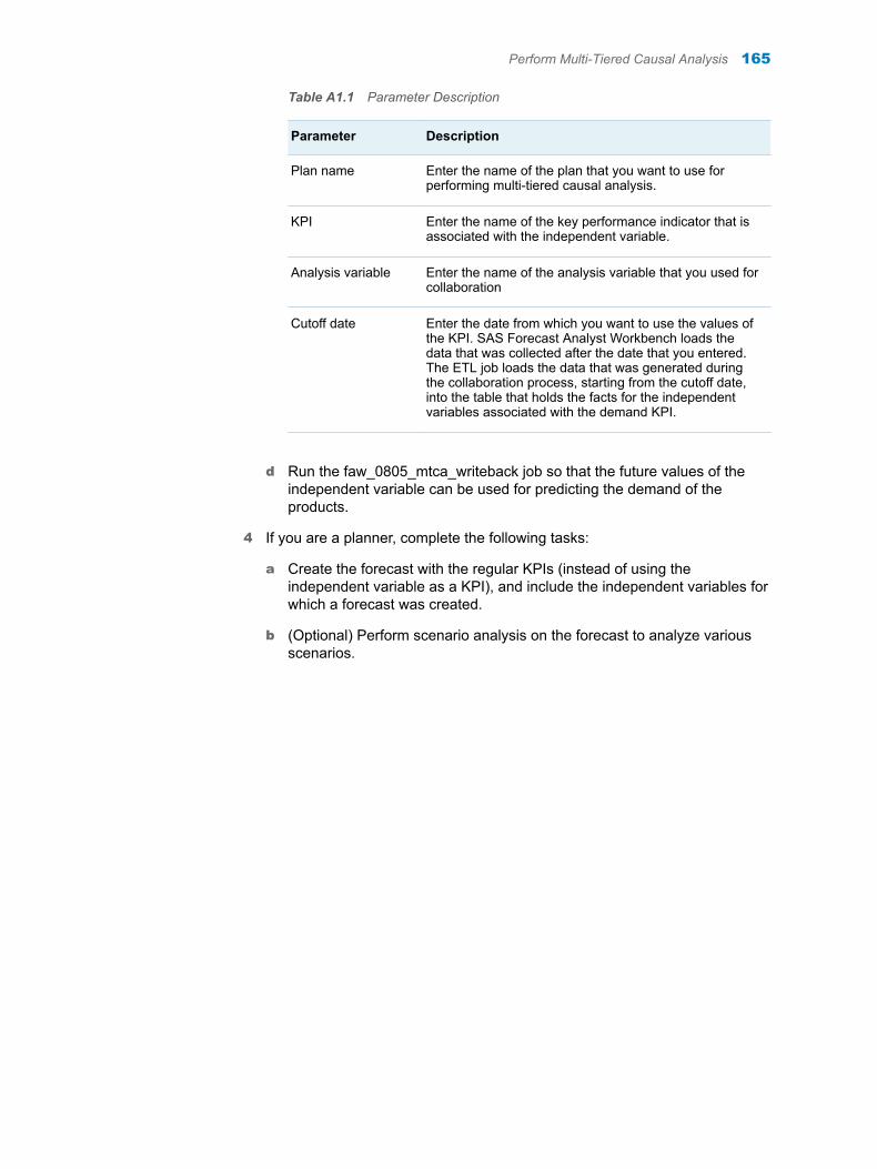
Table A1.1 Parameter Description
Parameter Description
Plan name Enter the name of the plan that you want to use for performing multi-tiered causal analysis.
KPI Enter the name of the key performance indicator that is associated with the independent variable.
Analysis variable Enter the name of the analysis variable that you used for collaboration
Cutoff date Enter the date from which you want to use the values of the KPI. SAS Forecast Analyst Workbench loads the data that was collected after the date that you entered. The ETL job loads the data that was generated during the collaboration process, starting from the cutoff date, into the table that holds the facts for the independent variables associated with the demand KPI.
d Run the faw_0805_mtca_writeback job so that the future values of the independent variable can be used for predicting the demand of the products.
4 If you are a planner, complete the following tasks:
a Create the forecast with the regular KPIs (instead of using the independent variable as a KPI), and include the independent variables for which a forecast was created.
b (Optional) Perform scenario analysis on the forecast to analyze various scenarios.
Perform Multi-Tiered Causal Analysis 165

166 Appendix 1 / Performing Multi-Tier Causal Analysis

Recommended ReadingHere is the recommended reading list for this title:
n SAS Forecast Server Procedures 14.1: User’s Guide
n SAS Forecast Studio 14.1: User’s Guide
n Demand-Driven Forecasting: A Structured Approach to Forecasting
n SAS Forecast Analyst Workbench 5.3: Administrator’s Guide
n SAS Forecast Analyst Workbench 5.3: Data Reference Guide
n SAS Financial Management 5.5: User’s Guide
n SAS Inventory Optimization Workbench 5.3: User’s Guide
For a complete list of SAS publications, go to sas.com/store/books. If you have questions about which titles you need, please contact a SAS Representative:
SAS BooksSAS Campus DriveCary, NC 27513-2414Phone: 1-800-727-0025Fax: 1-919-677-4444Email: [email protected] address: sas.com/store/books
167

168 Recommended Reading
Glossaryaccumulation
either of two processes that are used to convert a time series. (1) Accumulation converts a time series that has no fixed interval into a time series that does have a fixed interval (such as hourly or monthly). (2) Accumulation converts a time series that has a fixed interval into a time series with a lower frequency time interval (such as hourly into daily). Accumulation combines data within the same time interval into a summary value for that time period.
adjustment variableidentifies data that should be excluded before you perform a statistical analysis.
aggregationthe act or process of grouping data by using an operation that produces a statistic such as a sum, average, minimum, or maximum.
AICSee Akaike's information criterion.
Akaike's information criterion (AIC)a measure of the goodness of fit of an estimated statistical model that can be used to compare one model against another model. The model with the lowest AIC value is the best.
analytical base tablea highly denormalized data structure that is designed to build an analytical model or to generate scores based on an analytical model.
AR modelSee autoregressive model.
ARIMA modela general probabilistic model for stationary time series involving any combination of autoregressive (AR) and moving average (MA) parameters. ARIMA models involve differenced time series variables.
attributea property of an object, component, or other entity. Examples of attributes might be name, size, color, label, format, informat, data type, or length.
autoregressive model (AR model)one of two fundamental types of probabilistic models for stationary time series data in the Box-Jenkins approach. Autoregressive models involve parameter estimates associated with lagged time series values.
169
batch modea noninteractive method of running SAS programs by which a file (containing SAS statements along with any necessary operating system commands) is submitted to the batch queue of the operating environment for execution.
bill of material (BOM)information consisting of details about child products that are related to particular parent products. Information is stored only for child products that can be sold separately. The BOM information is stored in the form of a relationship between the parent and child products.
BOMSee bill of material.
bottom-up method of reconciliationa reconciliation method that uses the forecasts at the lowest level of the hierarchy to adjust forecasts for the higher levels in the hierarchy. See also middle-out method of reconciliation.
capabilityan application feature that is under role-based management. Typically, a capability corresponds to a menu item or button. For example, a Report Creation capability might correspond to a New Report menu item in a reporting application. Capabilities are assigned to roles.
client tierthe portion of a distributed application that requests services from the server tier. The client tier typically includes a graphical user interface and uses a relatively small amount of disk space.
comma-separated values formatSee CSV format.
CSV format (comma-separated values format)a simple file format in which each line represents one entry, record, row, or observation in a database management system (or in some other application), and in which data values are separated by commas.
data marta subset of the data in a data warehouse. A data mart is optimized for a specific set of users who need a particular set of queries and reports.
data setSee SAS data set.
data tierin a SAS business intelligence system, the architectural layer in which SAS runs data-handling programs (including the logical servers for workspace and stored process servers). The data tier includes transformations, error tables, and jobs.
data warehouse (warehouse)a collection of pre-categorized data that is extracted from one or more sources for the purpose of query, reporting, and analysis. Data warehouses are generally used for storing large amounts of data that originates in other corporate applications or that is extracted from external data sources.
170 Glossary

deployment planinformation about what software should be installed and configured on each machine in a SAS deployment. A deployment plan is stored in a plan.xml file.
digital certificatean electronic document that binds a public key to an individual or an organization. A digital certificate usually contains a public key, a user's name, an expiration date, and the name of a Certification Authority.
dimensiona data element that categorizes values in a data set into non-overlapping categories that can be used to group, filter, and label the data in meaningful ways. Hierarchies within a dimension typically represent different groupings of information that pertains to a single concept. For example, a Time dimension might consist of two hierarchies: (1) Year, Month, and Date, and (2) Year, Week, and Day.
disaggregation methoda method that specifies how the forecasts in the lower level of the hierarchy are reconciled when the reconciliation method is top-down or middle-out. The disaggregation method can reconcile the forecasts in either of the following ways: (1) by using the proportion that each lower-level forecast contributes to the higher-level forecast; or (2) by splitting equally the difference between the higher-level forecast and the lower-level forecasts. See also middle-out method of reconciliation.
drill downto explore data and access information by moving from summary information to more detailed data from which the summary is derived. For example, you could click folders in a hierarchy from the top downwards to find a specific file. Drilling down provides a method of exploring multidimensional data by moving from one level of detail to the next.
ETLSee extract, transform, load.
ETL joba set of instructions that is used to specify ETL processes that are needed to create output.
eventan incident that disrupts the normal flow of any process that generates the time series. Examples of events are holidays, retail promotions, and natural disasters.
explanatory variableSee independent variable.
exponential smoothinga forecasting technique using exponentially declining weights to produce a weighted moving average of time series values. The parameter estimates for trend models are updated using this method to reflect changes in the data. Double and triple exponential smoothing can be performed by repeatedly smoothing the smoothed values.
Glossary 171
extract, transform, load (ETL)a data warehousing process in which data is extracted from outside sources, transformed according to operational and quality needs, and loaded into a target database.
facta single piece of factual information in a data table. For example, a fact can be an employee name, a customer's phone number, or a sales amount. It can also be a derived value such as the percentage by which total revenues increased or decreased from one year to the next.
forecasta numerical prediction of a future value for a specified time period.
forecasting intervalthe frequency at which data should be forecasted.
foreign keythe primary key of one data structure that is placed into a related data structure to represent a relationship between those data structures. A foreign key resolves relationships and supports navigation among data structures.
form seta set of identically structured data-entry forms that enable users to enter data into the underlying cycle. Each member of the form set's target hierarchy has a form. See also hierarchy.
granularitythe relative level of detail that a data item represents. From the top of a dimension to the bottom, granularity increases. For example, in a Time dimension that consists of a Year-Month-Day hierarchy, Month is more granular than Year, and Day is more granular than Month.
groupSee user group.
hierarchyan arrangement of related objects into levels that are based on parent-child relationships. Members of a hierarchy are arranged from more general to more specific. See also dimension.
histograma bar chart that displays the observed frequencies of data that have been divided into contiguous, equally spaced intervals. The heights of the bars indicate the relative frequency of observations in each bin.
horizonthe number of intervals into the future, beyond a base date, for which analyses and predictions are made.
independent variable (predictor variable, explanatory variable)a variable that represents the value that is being manipulated or changed, in order to determine its relationship to some other observed phenomenon (the dependent variable). For example, in a study to determine the effects of a vitamin on lifespan, vitamin C might be an independent variable, and lifespan would be the dependent variable.
172 Glossary
Integrated Object Model (IOM)the set of distributed object interfaces that make SAS software features available to client applications when SAS is executed as an object server.
IOMSee Integrated Object Model.
IOM bridgea software component of SAS Integration Technologies that enables Java clients and Windows clients to access an IOM server.
key performance indicator (KPI)a type of measurement that evaluates the success of an organization or of an activity in which it engages. Success might be defined as the periodic achievement of one or more operational goals, or in terms of progress toward strategic goals. Results are usually measured at regular intervals, against threshold values that are carefully selected according to their importance.
KPISee key performance indicator.
leafin a tree diagram, any segment that is not further segmented. The final leaves in a tree are called terminal nodes.
life cycleSee product life cycle.
localea setting that reflects the language, local conventions, and culture for a geographic region. Local conventions can include specific formatting rules for paper sizes, dates, times, and numbers, and a currency symbol for the country or region. Some examples of locale values are French_Canada, Portuguese_Brazil, and Chinese_Singapore.
logical data modela framework into which engines fit information for processing by SAS. This data model is a logical representation of data or files, not a physical structure.
MAPESee mean absolute percent error.
mean absolute percent error (MAPE)the average of the absolute percentage errors.
metadatadescriptive data about data that is stored and managed in a database, in order to facilitate access to captured and archived data for further use.
metadata repositorya collection of related metadata objects, such as the metadata for a set of tables and columns that are maintained by an application.
Glossary 173

metadata servera server that provides metadata management services to one or more client applications.
middle tierin a SAS business intelligence system, the architectural layer in which web applications and related services execute. The middle tier receives user requests, applies business logic and business rules, interacts with processing servers and data servers, and returns information to users.
middle-out method of reconciliationa reconciliation method that combines the bottom-up method above the reconciliation level and the top-down method below the reconciliation level. When a hierarchy has more than one middle level, you need to specify which of those levels to use as the reconciliation level. The forecasts at the reconciliation level are used to generate forecasts for both the higher and lower levels. See also bottom-up method of reconciliation.
moving averagean average of a specified number of consecutive values that move according to the current observation.
object spawner (spawner)a program that instantiates object servers that are using an IOM bridge connection. The object spawner listens for incoming client requests for IOM services.
parallel executionSee parallel processing.
parallel processing (parallel execution)a method of processing that divides a large job into multiple smaller jobs that can be executed simultaneously on multiple CPUs.
permissionthe type of access that a user or group has to a resource. The permission defines what the user or group can do with the resource. Examples of permissions are ReadMetadata and WriteMetadata.
predictor variableSee independent variable.
primary keya set of one or more attributes that uniquely identifies a single occurrence in a data structure, such as a row in a table.
product life cycle (life cycle)the progression of a product through a sequence of stages from introduction to growth, maturity, and decline. The product life cycle is affected by changes in how the product is marketed.
reconciliation methodthe method that specifies the level in the hierarchy where the process of reconciliation starts. The following reconciliation methods are available: bottom-up method, middle-out method, and top-down method.
174 Glossary

retained keya numeric column in a dimension table that is combined with a begin-date column to make up the primary key.
RMSESee root mean square error.
role (user role)a set of capabilities within an application that are targeted to a particular group of users.
root mean square error (RMSE)the square root of the mean square error. It is used as an estimate of the standard deviation of the response variable.
SAS data set (data set)a file whose contents are in one of the native SAS file formats. There are two types of SAS data sets: SAS data files and SAS data views.
SAS Deployment Wizarda cross-platform utility that installs and initially configures many SAS products. Using a SAS installation data file and, when appropriate, a deployment plan for its initial input, the wizard prompts the customer for other necessary input at the start of the session, so that there is no need to monitor the entire deployment.
SAS environmentan abstraction for treating a deployed set of SAS software components as one entity. A SAS environment can be regarded as a virtual container that components are deployed in. A SAS environment spans the logic (middle) and data tiers to provide a single point of access for SAS client applications in the presentation tier. Via a SAS environment, an application can access component-supplied services for everything from authentication to specialized business functions without exposing application users to technical deployment details like host names and port numbers. A SAS environment always represents a complete, self-contained, fully functioning deployment of SAS products. A typical SAS environment includes SAS Metadata Server, SAS Workspace Server, Web Report Studio, an object spawner, a Java application server, and a SAS solution such as Financial Management.
SAS installation data (SID)the license information and data, including the setinit, that are required for a customer installation.
SAS Management Consolea Java application that provides a single user interface for performing SAS administrative tasks.
SAS Software Depota file system that consists of a collection of SAS installation files that represents one or more orders. The depot is organized in a specific format that is meaningful to the SAS Deployment Wizard, which is the tool that is used to install and initially configure SAS. The depot contains the SAS Deployment Wizard executable, one or more deployment plans, a SAS installation data file, order data, and product data.
Glossary 175

SAS Stored Process (stored process)a SAS program that is stored on a server and defined in metadata, and which can be executed by client applications.
SAS Workspace Servera SAS server that provides access to SAS Foundation features such as the SAS programming language and SAS libraries.
SBCSee Schwarz's Bayesian Criterion.
Schwarz's Bayesian Criterion (SBC)a statistical criterion for model selection that uses a parametric method to overcome an overtraining problem that can result if too many parameters are used in a model.
seasonalitya regular change in time series data values that occurs at the same point in each time cycle.
seedto use existing data (such as historical, planning, or forecasting data) to populate initial values in a worksheet.
server tierin a SAS business intelligence system, the tier in which the SAS servers execute. Examples of such servers are the SAS Metadata Server, the SAS Workspace Server, the SAS Pooled Workspace Server, the SAS Stored Process Server, and the SAS OLAP Server. These servers are typically accessed either by clients or by web applications that are running in the middle tier.
SIDSee SAS installation data.
slicea subset of data from a cube, where the data in the slice pertains to one or more members of one or more dimensions. For example, from a cube that contains data about customer feedback, one slice might pertain to feedback on one particular product (one member of the Product dimension). Another slice might pertain to feedback on that product from customers residing in particular geographic areas who submitted their feedback during a certain time period (one member of the Product dimension, multiple members of the Geography dimension, one or more members of the Time dimension).
solution data layeran intermediate layer of tables provided by the solution to save the customer source data in the required manner.
source systemthe type of database from which operational loss data originates or to which it is being exported.
spawnerSee object spawner.
176 Glossary

staged tablea type of table that contains data that has been extracted from an input data store and transformed into a standard form for further transformation. A staged table is defined in metadata from a template table, which, after it is used, exists in physical form.
stored processSee SAS Stored Process.
stored process servera server that can execute SAS programs as required by one or more client applications. See also SAS Stored Process.
surrogate keya numeric column in a dimension table that is the primary key of that table.
time seriesan ordered sequence of values of a variable that are observed at equally spaced time intervals.
time series datatimestamped data collected over time at a particular frequency. Some examples of time series data are web visits per hour, sales per month, and calls per day.
top-down method of reconciliationa reconciliation method that uses the forecasts at the highest level of the hierarchy to adjust the forecasts for the lower levels. See also bottom-up method of reconciliation.
transactional datatimestamped data collected over time at no particular frequency. Some examples of transactional data are point-of-sale data, inventory data, call center data, and trading data.
transformationin the DATA Step Graphics Interface (DSGI), a mapping of the window coordinates to the viewport coordinates.
trenda long-term consistent change, as measured by time series values.
Unicode Transformation Format 8See UTF-8.
user group (group)an organization of user roles within an entity organization. User groups contain the roles and access rights for the individuals assigned to the group.
user roleSee role.
UTF-8 (Unicode Transformation Format 8)a method for converting 16-bit Unicode characters to 8-bit characters. This format supports all of the world's languages, including those that use non-Latin 1 characters.
Glossary 177

warehouseSee data warehouse.
workflowa series of tasks, together with the participants and the logic that is required to execute the tasks. A workflow includes policies, status values, and data objects.
178 Glossary

IndexA
analysiscreate 102custom 101delete 106edit 105explore output 106share 105three-stage modeling 103
analysis variablesconfigure 117
ARIMAX 45attributes
common 16, 89product-specific 16, 89
B
batch mode 31
C
candidate productsdefine 84select 84
child products 67clusters
define 87select 91
collaborationcomplete 121configure analysis variables 117initialize 121initiate 118overview 109provide inputs 120
common attributes 16, 89copy
forecasts 28create
analysis 102forecasts 13modeling projects 55
new product forecasting project 86custom analysis 101cycle series 93
D
decomposition 87delete
analysis 106forecasts 28modeling projects 79new product forecasting project 96
demandcompare 131, 132explore 132tolerance limit 132
E
editanalysis 105forecasts 27
edit parametersof a forecast 44of multiple time series 44
ESM 48evaluate
time series 45events
combined 21guidelines 21simple 21
explore demandoverview 131
F
forecastexplore 131improve 38, 43, 55, 71review 93
forecast leaf leveldefine 17
179
forecastsaccept 59copy 28create 13define objective 14delete 28diagnose 42, 43edit 27edit parameters 43overview 5reconcile 57rediagnose 57refresh 29reorganize hierarchy 17rerun forecast 59schedule in batch 31select hierarchical values 15select hierarchy levels 14specify common attributes 16specify other parameters 18specify product-specific attributes
16statuses 32update 30
form setscreate 118
formspublish 120
G
guidelinesfor events 21for modeling projects 77
H
hierarchical values 15hierarchy levels 14
define 14histogram 89
I
independent variables 24, 49, 65
K
KPI 14
M
MAPE 38, 66modeling projects
create 55delete 79guidelines 77open 78overview 71promote 79refresh 78statuses 75workflow 72
modelsARIMAX 45compare 55ESM 48select default model 55select for a new product 92UCM 47
N
new product forecasting projectsassign to a forecast 94create 86define candidate products 84define relationships 84delete 96overview 83reduction method 87review forecasts 93select candidate products 84select models 92select surrogate products 91statuses 96workflow 84
O
openmodeling projects 78
P
parametersARIMAX model 45combined model 52edit 43ESM model 48evaluate 45
180 Index

forecast 52model selection 50UCM model 47
periodicity 18periodicity mismatch 94plans
create 113delete 124edit 123refresh 125
predicted valuescompare 38, 131, 132explore 131
prediction error 38, 65product-specific attributes 16, 89profile series 93promote
modeling projects 79
R
reconciliation leveldefine 17
reconciliation methodbottom-up 17middle-up 17top-down 17
reduction methoddecomposition 87smoothing 87
refreshforecasts 29mmodeling projects 78
reorganize hierarchy 17reports 159
create 160edit 159view 159
RMSE 38, 66
S
SAS for Demand-Driven Planning and Optimization 3
scenario analysisexport values 139overview 135perform 138
scheduleforecasts in batch mode 31
seasonalityadjust 91define 87
shareanalysis 105
smoothing 87surrogate products
select 91
T
three-stage modelinganalysis 103independent variables 103
time seriesedit parameters 44evaluate 45filter 63plot 90
time zone 9
U
UCM 47user interface
define preferences 8understand time zone 9
Index 181

182 Index


![HCL Analyst And advisor's day-US V1.1 in attrition ... COPC SAS 70 Compliant OE ... Microsoft PowerPoint - HCL Analyst And advisor's day-US V1.1 [Compatibility Mode] Author: rohankv](https://static.fdocuments.in/doc/165x107/5aeba8067f8b9ad73f8ebcf4/hcl-analyst-and-advisors-day-us-v11-in-attrition-copc-sas-70-compliant-oe.jpg)