(F)MRI Physics(F)MRI PhysicsWith Hardly Any MathWith Hardly Any Math**

(F)MRI Physics(F)MRI PhysicsWith Hardly Any MathWith Hardly Any Math**

Robert W Cox, PhDRobert W Cox, PhDScientific and Statistical Computing Core

National Institute of Mental Health

Bethesda, MD USA

*Equations can be supplied to the inquiring student*Equations can be supplied to the inquiring student

MRI Cool (and Useful) Pictures

2D slices extracted from a 3D image2D slices extracted from a 3D image[resolution about 1[resolution about 1111 mm]1 mm]

axialaxial coronalcoronal sagittalsagittal

Synopsis of MRI 1) Put subject in big magnetic field (leave him there)

2) Transmit radio waves into subject [about 3 ms]

3) Turn off radio wave transmitter

4) Receive radio waves re-transmitted by subject Manipulate re-transmission with magnetic fields during

this readout interval [10-100 ms: MRI is not a snapshot]

5) Store measured radio wave data vs. time Now go back to 2) to get some more data

6) Process raw data to reconstruct images

7) Allow subject to leave scanner (this is optional)

Components of Lectures

1) Magnetic Fields and Magnetization

2) Fundamental Ideas about the NMR RF Signal

3) How to Make an Image

4) Some Imaging Methods

5) The Concept of MRI Contrast

6) Functional Neuroimaging with MR

}} NMRNMRPhysicsPhysics

}} MRIMRIPrinciplesPrinciples

}} MakingMakingUsefulUsefulImagesImages

Part the FirstPart the First

Magnetic Fields;Magnetic Fields;Magnetization of the Subject;Magnetization of the Subject;

How the Two InteractHow the Two Interact

Magnetic Fields Magnetic fields create the substance we “see”:

magnetization of the H protons in H2O

Magnetic fields also let us manipulate magnetization so that we can make a map [or image] of its density inside the body’s tissue

Static fields change slowly (not at all, or only a few 1000 times per second) Main field; gradient fields; static inhomogeneities

RF fields oscillate at Radio Frequencies (tens of millions of times per second) transmitted radio waves into subject received signals from subject

Vectors and Fields Magnetic field B and magnetization M are vectors:

Quantities with direction as well as size Drawn as arrows .................................... Another example: velocity is a vector (speed is its size)

A field is a quantity that varies over a spatial region: e.g., velocity of wind at each location in the atmosphere

Magnetic field exerts torque to line magnets up in a given direction direction of alignment is direction of B torque proportional to size of B [units=Tesla, Gauss=10–4 T]

B0 = Big Field Produced by Main Magnet

Purpose is to align H protons in H2O (little magnets)

[Little magnets lining up with external lines of force]

[Main magnet and some of its lines of force]

Small B0 produces small net magnetization M

Thermal motions try to randomize alignment of proton magnets

Larger B0 produces larger net magnetization M, lined up with B0

Reality check: 0.0003% of protons aligned per Tesla of B0

If M is not parallel to B, thenit precesses clockwise aroundthe direction of B.

However, “normal” (fully relaxed) situation has M parallel to B, which means there won’t be anyprecession

Precession of Magnetization M Magnetic field causes M to rotate (or precess) about the

direction of B at a frequency proportional to the size of B — 42 million times per second (42 MHz), per Tesla of B

N.B.: part of M parallel to B (Mz) does not precess

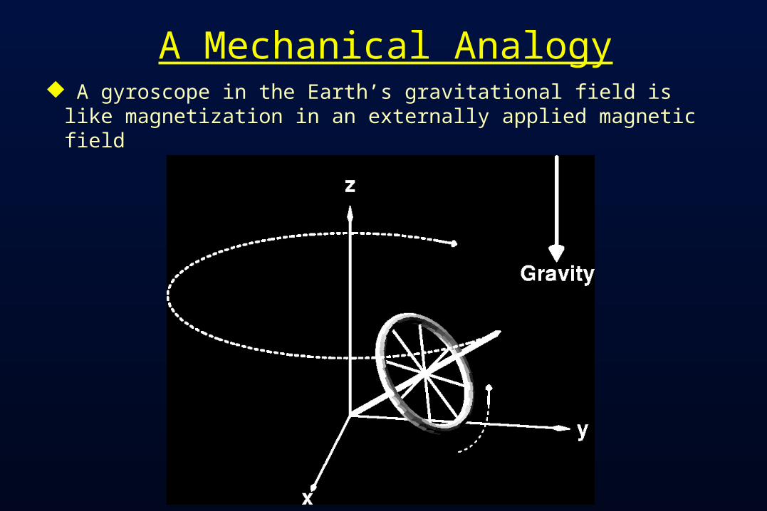
A Mechanical Analogy A gyroscope in the Earth’s gravitational field is like

magnetization in an externally applied magnetic field

How to Make M not be Parallel to B? A way that does not work:

Turn on a second big magnetic field B1 perpendicular to main B0 (for a few seconds)

Then turn B1 off; M is now not parallel to magnetic field B0

This fails because cannot turn huge (Tesla) magnetic fields on and off quickly

But it contains the kernel of the necessary idea:

A magnetic field B1 perpendicular to B0

B0

B1

B0+B1

M would drift over to be aligned with sum of B0 and B1

The effect of the tiny B1 is to cause M to spiral away from the direction of the static B field B110–4 Tesla This is called resonance If B1 frequency is not close to resonance, B1 has no effect

B1 = Excitation (Transmitted) RF Field Left alone, M will align itself with B in about 2–3 s So don’t leave it alone: apply (transmit) a magnetic

field B1 that fluctuates at the precession frequency and points perpendicular to B0

Time = 2–4 ms

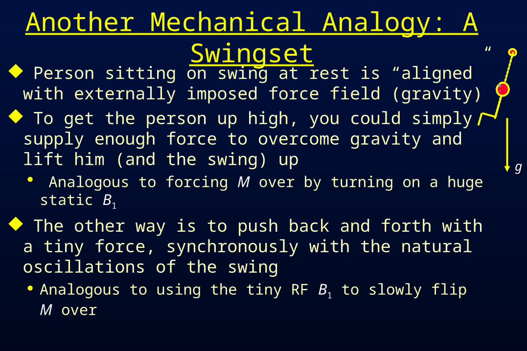
Another Mechanical Analogy: A Swingset Person sitting on swing at rest is “aligned” with

externally imposed force field (gravity)

To get the person up high, you could simply supply enough force to overcome gravity and lift him (and the swing) up Analogous to forcing M over by turning on a huge static B1

The other way is to push back and forth with a tiny force, synchronously with the natural oscillations of the swing Analogous to using the tiny RF B1 to slowly flip M over

gg

Readout RF

When excitation RF is turned off, M is left pointed off at some angle to B0 [flip angle]

Precessing part of M [Mxy] is like having a magnet rotating around at very high speed (at RF frequencies)

Will generate an oscillating voltage in a coil of wires placed around the subject — this is magnetic induction

This voltage is the RF signal whose measurements form the raw data for MRI At each instant in time, can measure one voltage V(t), which

is proportional to the sum of all transverse Mxy inside the coil Must find a way to separate signals from different regions

But before I talk about localization (imaging):

Part the SecondPart the Second

Fundamental IdeasFundamental Ideasaboutabout

the NMR RF Signalthe NMR RF Signal

Relaxation: Nothing Lasts Forever

In absence of external B1, M will go back to being aligned with static field B0 — this is called relaxation

Part of M perpendicular to B0 shrinks [Mxy]

This part of M is called transverse magnetization

It provides the detectable RF signal

Part of M parallel to B0 grows back [Mz] This part of M is called longitudinal magnetization Not directly detectable, but is converted into

transverse magnetization by externally applied B1

Relaxation Times and Rates Times: ‘T’ in exponential laws like e–t/T

Rates: R = 1/T [so have relaxation like e–Rt]

T1: Relaxation of M back to alignment with B0

Usually 500-1000 ms in the brain [lengthens with bigger B0]

T2: Intrinsic decay of the transverse magnetization over a microscopic region ( 5-10 micron size) Usually 50-100 ms in the brain [shortens with bigger B0]

T2*: Overall decay of the observable RF signal over a macroscopic region (millimeter size) Usually about half of T2 in the brain [i.e., faster relaxation]

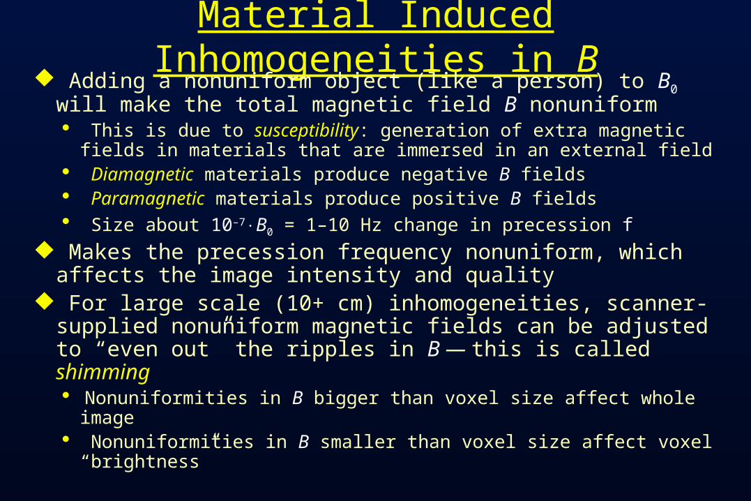
Material Induced Inhomogeneities in B Adding a nonuniform object (like a person) to B0 will make the

total magnetic field B nonuniform This is due to susceptibility: generation of extra magnetic fields in

materials that are immersed in an external field Diamagnetic materials produce negative B fields Paramagnetic materials produce positive B fields Size about 10–7B0 = 1–10 Hz change in precession f

Makes the precession frequency nonuniform, which affects the image intensity and quality

For large scale (10+ cm) inhomogeneities, scanner-supplied nonuniform magnetic fields can be adjusted to “even out” the ripples in B — this is called shimming Nonuniformities in B bigger than voxel size affect whole image Nonuniformities in B smaller than voxel size affect voxel “brightness”

Frequency and Phase RF signals from different regions that are at

different frequencies will get out of phase and thus tend to cancel out Phase = the t in cos(t) [frequency f = /2]

Sum of 500 Cosines with Random Frequencies

Starts off large when all phases are about equal

High frequency gray curve is at the average frequency

Decays away as different components get different phases

Transverse Relaxation and NMR Signal Random frequency differences inside intricate tissue

environment cause RF signals (from Mxy) to dephase Measurement = sum of RF signals from many places Measured signal decays away over time [T2*40 ms at 1.5 T] At a microscopic level (microns), Mxy signals still exist; they

just add up to zero when observed from outside (at the RF coil)

Contents of tissue can affect local magnetic field Signal decay rate depends on tissue structure and material Measured signal strength will depend on tissue details If tissue contents change, NMR signal will change e.g., oxygen level in blood affects signal strength

Hahn Spin Echo: Retrieving Lost Signal Problem: Mxy rotates at different rates in different spots

Solution: take all the Mxy’s that are ahead and make them get behind (in phase) the slow ones After a while, fast ones catch up to slow ones re-phased!

Fast & slowFast & slowrunnersrunners

Magically “beam”Magically “beam”runners across trackrunners across track

Let them run theLet them run thesame time as beforesame time as before

The “magic” trick: inversion of the magnetization M

Apply a second B1 pulse to produce a flip angle of 180 about the y-axis (say)

Time between first and second B1 pulses is called TI

“Echo” occurs at time TE = 2TI

Spin EchoSpin Echo::

ExciteExcite

PrecessPrecess & dephase& dephase

180180 flip flip

PrecessPrecess & rephase& rephase

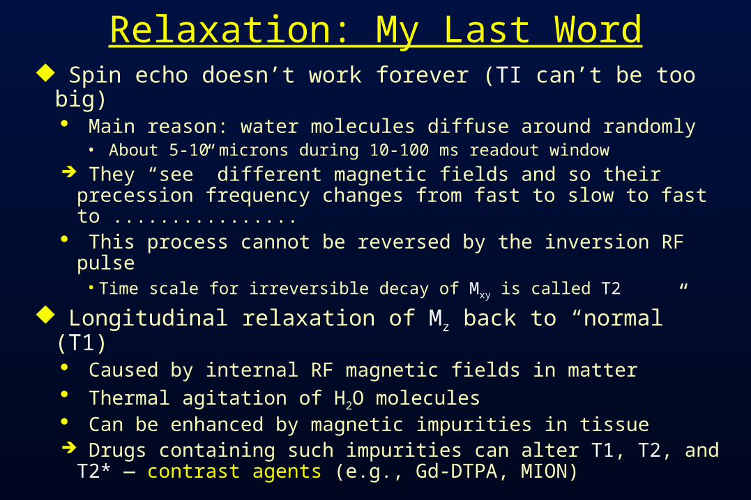
Relaxation: My Last Word Spin echo doesn’t work forever (TI can’t be too big)

Main reason: water molecules diffuse around randomly• About 5-10 microns during 10-100 ms readout window

They “see” different magnetic fields and so their precession frequency changes from fast to slow to fast to ................

This process cannot be reversed by the inversion RF pulse• Time scale for irreversible decay of Mxy is called T2

Longitudinal relaxation of Mz back to “normal” (T1) Caused by internal RF magnetic fields in matter Thermal agitation of H2O molecules Can be enhanced by magnetic impurities in tissue Drugs containing such impurities can alter T1, T2, and T2*

— contrast agents (e.g., Gd-DTPA, MION)

Part the ThirdPart the Third

LocalizationLocalizationof theof the

NMR Signal,NMR Signal,oror,,

How to Make ImagesHow to Make Images

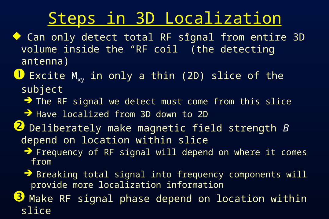
Steps in 3D Localization Can only detect total RF signal from entire 3D volume

inside the “RF coil” (the detecting antenna)

Excite Mxy in only a thin (2D) slice of the subject The RF signal we detect must come from this slice Have localized from 3D down to 2D

Deliberately make magnetic field strength B depend on location within slice Frequency of RF signal will depend on where it comes from Breaking total signal into frequency components will

provide more localization information

Make RF signal phase depend on location within slice

Spatially Nonuniform B: Gradient Fields Extra static magnetic fields (in addition to B0) that

vary their intensity in a linear way across the subject

Precession frequency of M varies across subject This is called frequency encoding — using a

deliberately applied nonuniform field to make the precession frequency depend on location

x-axis

f60 KHz

Left = –7 cm Right = +7 cm

Gx = 1 Gauss/cm = 10 mTesla/m = strength of gradient field

Centerfrequency

[63 MHz at 1.5 T]

Exciting Mxy in a Thin Slice of Tissue

Readout Localization After RF pulse (B1) ends, acquisition (readout) of

NMR RF signal begins During readout, gradient field perpendicular to slice

selection gradient is turned on Signal is sampled about once every microsecond, digitized,

and stored in a computer• Readout window ranges from 5–100 milliseconds (can’t be longer

than about 2T2*, since signal dies away after that)

Computer breaks measured signal V(t) into frequency components v(f ) — using the Fourier transform

Since frequency f varies across subject in a known way, we can assign each component v(f ) to the place it comes from

Image Resolution (in Plane) Spatial resolution depends on how well we can

separate frequencies in the data V(t) Resolution is proportional to f = frequency accuracy Stronger gradients nearby positions are better separated

in frequencies resolution can be higher for fixed f Longer readout times can separate nearby frequencies

better in V(t) because phases of cos(ft) and cos([f+f]t) will have longer to separate: f = 1/(readout time)

The Last Dimension: Phase Encoding Slice excitation provides one localization dimension Frequency encoding provides second dimension The third dimension is provided by phase encoding:

We make the phase of Mxy (its angle in the xy-plane) signal depend on location in the third direction

This is done by applying a gradient field in the third direction ( to both slice select and frequency encode)

Fourier transform measures phase of each v(f ) component of V(t), as well as the frequency f

By collecting data with many different amounts of phase encoding strength, can break each v(f ) into phase components, and so assign them to spatial locations in 3D

Part the FourthPart the Fourth

Some Imaging MethodsSome Imaging Methods

The Gradient Echo

Spin echo: when “fast” regions get ahead in phase, make them go to the back and catch up

Gradient echo: make “fast” regions become “slow” and vice-versa Only works when different precession rates are due to

scanner-supplied gradient fields, so we can control them Turn gradient field on with negative slope for a while, then

switch it to have positive slope What was fast becomes slow (and vice-versa) and after a

time, the RF signal phases all come back together The total RF signal becomes large at that time (called TE)

MRI Pulse Sequence for Gradient Echo Imaging

Illustratessequence ofevents duringscanning

As shown, this method(FLASH)takes 35 msper RF shot,so would take2.25 s for a6464 image

Why Use the Gradient Echo? Why not readout without negative frequency encoding?

Purpose: delay the time of maximum RF signal Occurs at t = TE after the RF pulse During this time, magnetization M will evolve not only due to

externally imposed gradients, but also due to microscopic (sub-voxel) structure of magnetic field inside tissue

Delaying readout makes signal more sensitive to these internal details

Resulting image intensity I(x,y) depends strongly on T2* at each location (x,y) Most sensitive if we pick TE average T2*

MRI Pulse Sequence for Spin Echo Imaging

Why Use the Spin Echo? Purpose: re-phase the NMR signals that are lost due to

sub-voxel magnetic field spatial variations Resulting image intensity I(x,y) depends strongly on T2

at each location (x,y) Most sensitive if we pick TE average T2

SE images depend mostly on tissue properties at the 5 micron and smaller level (molecular to cellular sizes) = diffusion scale of H2O in tissue during readout

GE images depend on tissue properties over all scales up to voxel dimensions (molecular to cellular to structural)

Echo Planar Imaging (EPI)

Methods shown earlier take multiple RF shots to readout enough data to reconstruct a single image Each RF shot gets data with one value of phase encoding

If gradient system (power supplies and gradient coil) are good enough, can read out all data required for one image after one RF shot Total time signal is available is about 2T2* [80 ms]

Must make gradients sweep back and forth, doing all frequency and phase encoding steps in quick succession

Can acquire 10-20 low resolution 2D images per second

GE-EPI Pulse Sequence

Actually haveActually have64 (or more)64 (or more)freq. encodesfreq. encodesin one readoutin one readout(each one (each one << 1 1

ms)ms)

[only 13 freq.[only 13 freq.encodesencodes

shown here]shown here]

What Makes the Beeping Noise in EPI? Gradients are created by currents through wires in the

gradient coil — up to 100 Amperes

Currents immersed in a magnetic field have a force on them — the Lorentz force — pushing them sideways

Switching currents back and forth rapidly causes force to push back and forth rapidly

Force on wires causes coil assembly to vibrate rapidly

Frequency of vibration is audio frequency about 1000 Hz = switching rate of frequency encode gradients scanner is acting like a (low-fidelity) loudspeaker

Other Imaging Methods Can “prepare” magnetization to make readout signal

sensitive to different physical properties of tissue Diffusion weighting (scalar or tensor) Magnetization transfer (sensitive to proteins in voxel) Flow weighting (bulk movement of blood) Perfusion weighting (blood flow into capillaries) Temperature; T1, T2, T2*; other molecules than H2O

Can readout signal in many other ways Must program gradients to sweep out some region in k-

space = coordinates of phase/frequency

Example: spiral imaging (from Stanford)

tdGtk

0)()(

Part the FifthPart the Fifth

Image ContrastImage Contrastandand

Imaging ArtifactsImaging Artifacts

The Concept of Contrast (or Weighting) Contrast = difference in RF signals — emitted by

water protons — between different tissues Example: gray-white contrast is possible because

T1 is different between these two types of tissue

Types of Contrast Used in Brain FMRI T1 contrast at high spatial resolution

Technique: use very short timing between RF shots (small TR) and use large flip angles

Useful for anatomical reference scans 10 minutes to acquire 256256128 volume 1 mm resolution

T2 (spin-echo) and T2* (gradient-echo) contrast Useful for functional activation studies 2-4 seconds to acquire 646420 volume 4 mm resolution [better is possible with better gradient system,

and a little longer time per volume]

Other Interesting Types of Contrast Perfusion weighting: sensitive to capillary flow

Diffusion weighting: sensitive to diffusivity of H2O Very useful in detecting stroke damage Directional sensitivity can be used to map white matter tracts

Flow weighting: used to image blood vessels (MR angiography)

Brain is mostly WM, GM, and CSF Each has different value of T1 Can use this to classify voxels by tissue type

Magnetization transfer: provides indirect information about H nuclei that aren’t in H2O (mostly proteins)

Imaging Artifacts MR images are computed from raw data V(t)

Assumptions about data are built into reconstruction methods Magnetic fields vary as we command them to The subject’s protons aren’t moving during readout or

between RF excitations All RF signal actually comes from the subject

Assumptions aren’t perfect Images won’t be reconstructed perfectly Resulting imperfections are called artifacts:

• Image distortion; bleed-through of data from other slices; contrast depends on things you didn’t allow for; weird “zippers” across the image; et cetera ........

Part the SixthPart the Sixth

Functional NeuroimagingFunctional Neuroimaging

What is Functional MRI? 1991: Discovery that MRI-measurable signal

increases a few % locally in the brain subsequent to increases in neuronal activity (Kwong, et al.)

Cartoon of MRI signal in an “activated”

brain voxel

How FMRI Experiments Are Done Alternate subject’s neural state between 2 (or more)

conditions using sensory stimuli, tasks to perform, ... Can only measure relative signals, so must look for changes

Acquire MR images repeatedly during this process Search for voxels whose NMR signal time series

matches the stimulus time series pattern Signal changes due to neural activity are small

Need 50+ images in time series (each slice) takes minutes Other small effects can corrupt the results postprocess

Lengthy computations for image recon and temporal pattern matching data analysis usually done offline

Some Sample Data Time Series

16 slices, 6464 matrix, 68 repetitions (TR=5 s)

Task: phoneme discrimination: 20 s “on”, 20 s “rest”

graphs of 9 voxel time series

t

“Active” voxels

Graphs vs. time of 33 voxel regionOne Fast Image

Overlay on Anatomy

68 points in time 5 s apart; 16 slices of 6464 images

This voxel didnot respond

Colored voxels responded to the mentalstimulus alternation, whose pattern is shown in theyellow reference curve plotted in the central voxel

Why (and How) Does NMR Signal ChangeWith Neuronal Activity?

There must be something that affects the water molecules and/or the magnetic field inside voxels that are “active” neural activity changes blood flow

blood flow changes which H2O molecules are present and also changes the magnetic field

FMRI is thus doubly indirect from physiology of interest (synaptic activity) also is much slower: 4-6 seconds after neurons also “smears out” neural activity: cannot resolve 10-100

ms timing of neural sequence of events

Neurophysiological Changes & FMRI

There are 4 changes currently used in FMRI:

Increased Blood Flow New protons flow into slice More protons are aligned with B0

Equivalent to a shorter T1 (protons are realigned faster) NMR signal goes up [mostly in arteries]

Increased Blood Volume (due to increased flow) Total deoxyhemoglobin increases Magnetic field randomness increases NMR signal goes down [near veins and capillaries]

“Oversupply” of oxyhemoglobin after activation Total deoxyhemoglobin decreases Magnetic field randomness decreases NMR signal goes up [near veins and capillaries]

Increased capillary perfusion Inflowing spins exchange to parenchyma at capillaries Can be detected with perfusion-weighted imaging methods This is also the basis for 15O water-based PET

Deoxyhemo-globin is

paramagnetic(increases B)

Rest of tissueRest of tissueis diamagneticis diamagnetic(decreases (decreases BB))

Cartoon of Veins inside a Cartoon of Veins inside a VoxelVoxel

BOLD Contrast

BOLD = Blood Oxygenation Level Dependent

Amount of deoxyhemoglobin in a voxel determines how inhomogeneous that voxel’s magnetic field is at the scale of the blood vessels (and red blood cells)

Increase in oxyhemoglobin in veins after neural activation means magnetic field becomes more uniform inside voxel So NMR signal goes up (T2 and T2* are larger) Gradient echo: depends on vessels of all sizes Spin echo: depends only on smaller vessels

BOLD Sensitivity to Blood Vessel Sizes

Spatial Localization of Activity

Tradeoff : detectability (or scan time) vs. accuracy

Gradient echo Largest signal changes, but veins draining active area will

show “activity”, perhaps 10 mm away Due to very short T2*, very hard to use at ultra-high B0

Spin echo Smaller signal changes, but more localized to small vessels

Perfusion weighted imaging Even smaller signal changes, but potentially best localization “Difference of differences”

Physiological Artifacts Blood flow cycles up and down with cardiac cycle

Imaging rate slower than heartbeat means this looks like noise Brainstem also moves about 0.5 mm with cardiac cycle

Respiration causes periodic changes in blood oxygenation and magnetic field (due to movement of chest tissue)

Subject movements inside gradient coil cause signal changes Movements of imaged tissue are major practical problem Movements of tissue outside image (e.g., swallowing, speaking) can

change magnetic field inside image

Vasculature is different in each voxel, so BOLD response will be different even if neural activity is same Hard to compare response magnitude and timing between locations and

subjects

Structural Artifacts Un-shimmable distortions in B field cause protons to

precess in ways not allowed for Field is perturbed by interfaces between regions with

different susceptibilities, especially air-tissue boundaries Worst areas: above the nasal sinuses; near the ear canals

EP images will be warped in phase-encoding direction Can be partly corrected by measuring B field and using that

in reconstruction (the “VTE” method)

2D images will have signal dropout if through-slice field is not uniform Palliatives: shorten TE; use thinner slices