
Fluids dynamics and plasma physics P 1 Fluids dynamics and...
24
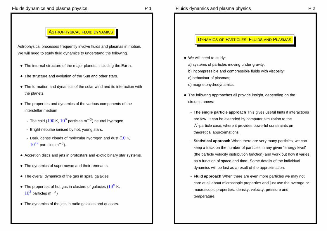
Fluids dynamics and plasma physics P1 ASTROPHYSICAL FLUID DYNAMICS Astrophysical processes frequently involve fluids and plasmas in motion. We will need to study fluid dynamics to understand the following. • The internal structure of the major planets, including the Earth. • The structure and evolution of the Sun and other stars. • The formation and dynamics of the solar wind and its interaction with the planets. • The properties and dynamics of the various components of the interstellar medium - The cold (100 K, 10 6 particles m -3 ) neutral hydrogen. - Bright nebulae ionised by hot, young stars. - Dark, dense clouds of molecular hydrogen and dust (10 K, 10 12 particles m -3 ). • Accretion discs and jets in protostars and exotic binary star systems. • The dynamics of supernovae and their remnants. • The overall dynamics of the gas in spiral galaxies. • The properties of hot gas in clusters of galaxies (10 8 K, 10 3 particles m -3 ) • The dynamics of the jets in radio galaxies and quasars. Fluids dynamics and plasma physics P2 D YNAMICS OF P ARTICLES,FLUIDS AND PLASMAS • We will need to study: a) systems of particles moving under gravity; b) incompressible and compressible fluids with viscosity; c) behaviour of plasmas; d) magnetohydrodynamics. • The following approaches all provide insight, depending on the circumstances: - The single particle approach This gives useful hints if interactions are few. It can be extended by computer simulation to the N -particle case, where it provides powerful constraints on theoretical approximations. - Statistical approach When there are very many particles, we can keep a track on the number of particles in any given “energy level” (the particle velocity distribution function) and work out how it varies as a function of space and time. Some details of the individual dynamics will be lost as a result of the approximation. - Fluid approach When there are even more particles we may not care at all about microscopic properties and just use the average or macroscopic properties: density; velocity; pressure and temperature.
Transcript of Fluids dynamics and plasma physics P 1 Fluids dynamics and...
Fluids dynamics and plasma physics P 1
ASTROPHYSICAL FLUID DYNAMICS
Astrophysical processes frequently involve fluids and plasmas in motion.
We will need to study fluid dynamics to understand the following.
• The internal structure of the major planets, including the Earth.
• The structure and evolution of the Sun and other stars.
• The formation and dynamics of the solar wind and its interaction with
the planets.
• The properties and dynamics of the various components of the
interstellar medium
- The cold (100 K, 106 particles m−3) neutral hydrogen.
- Bright nebulae ionised by hot, young stars.
- Dark, dense clouds of molecular hydrogen and dust (10 K,
1012 particles m−3).
• Accretion discs and jets in protostars and exotic binary star systems.
• The dynamics of supernovae and their remnants.
• The overall dynamics of the gas in spiral galaxies.
• The properties of hot gas in clusters of galaxies (108 K,
103 particles m−3)
• The dynamics of the jets in radio galaxies and quasars.
Fluids dynamics and plasma physics P 2
DYNAMICS OF PARTICLES, FLUIDS AND PLASMAS
• We will need to study:
a) systems of particles moving under gravity;
b) incompressible and compressible fluids with viscosity;
c) behaviour of plasmas;
d) magnetohydrodynamics.
• The following approaches all provide insight, depending on the
circumstances:
- The single particle approach This gives useful hints if interactions
are few. It can be extended by computer simulation to the
N -particle case, where it provides powerful constraints on
theoretical approximations.
- Statistical approach When there are very many particles, we can
keep a track on the number of particles in any given “energy level”
(the particle velocity distribution function) and work out how it varies
as a function of space and time. Some details of the individual
dynamics will be lost as a result of the approximation.
- Fluid approach When there are even more particles we may not
care at all about microscopic properties and just use the average or
macroscopic properties: density; velocity; pressure and
temperature.
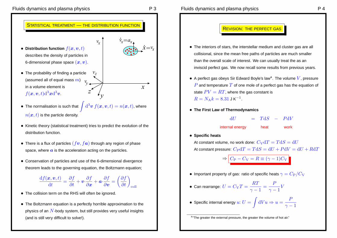
Fluids dynamics and plasma physics P 3
STATISTICAL TREATMENT — THE DISTRIBUTION FUNCTION
• Distribution function f(x, v, t)
describes the density of particles in
6-dimensional phase space (x, v).
• The probability of finding a particle
(assumed all of equal mass m)
in a volume element is
f(x, v, t)d3xd3v.
• The normalisation is such that
∫
d3v f(x, v, t) = n(x, t), where
n(x, t) is the particle density.
• Kinetic theory (statistical treatment) tries to predict the evolution of the
distribution function.
• There is a flux of particles (fv, fa) through any region of phase
space, where a is the acceleration acting on the particles.
• Conservation of particles and use of the 6-dimensional divergence
theorem leads to the governing equation, the Boltzmann equation;
df(x, v, t)
dt=
∂f
∂t+ v·∂f
∂x+ a·∂f
∂v=
(
∂f
∂t
)
coll
• The collision term on the RHS will often be ignored.
• The Boltzmann equation is a perfectly horrible approximation to the
physics of an N -body system, but still provides very useful insights
(and is still very difficult to solve!).
Fluids dynamics and plasma physics P 4
REVISION: THE PERFECT GAS
• The interiors of stars, the interstellar medium and cluster gas are all
collisional, since the mean free paths of particles are much smaller
than the overall scale of interest. We can usually treat the as an
inviscid perfect gas. We now recall some results from previous years.
• A perfect gas obeys Sir Edward Boyle’s lawa. The volume V , pressure
P and temperature T of one mole of a perfect gas has the equation of
state PV = RT , where the gas constant is
R = NAk = 8.31 J K−1.
• The First Law of Thermodynamics
dU = TdS − PdV
internal energy heat work
• Specific heats
At constant volume, no work done: CVdT = TdS = dU
At constant pressure: CPdT = TdS = dU + PdV = dU + RdT
⇒ CP − CV = R ≡ (γ − 1)CV
• Important property of gas: ratio of specific heats γ = CP/CV
• Can rearrange: U = CVT =RT
γ − 1=
P
γ − 1V
• Specific internal energy u: U =
∫
dV u ⇒ u =P
γ − 1
a“The greater the external pressure, the greater the volume of hot air.”
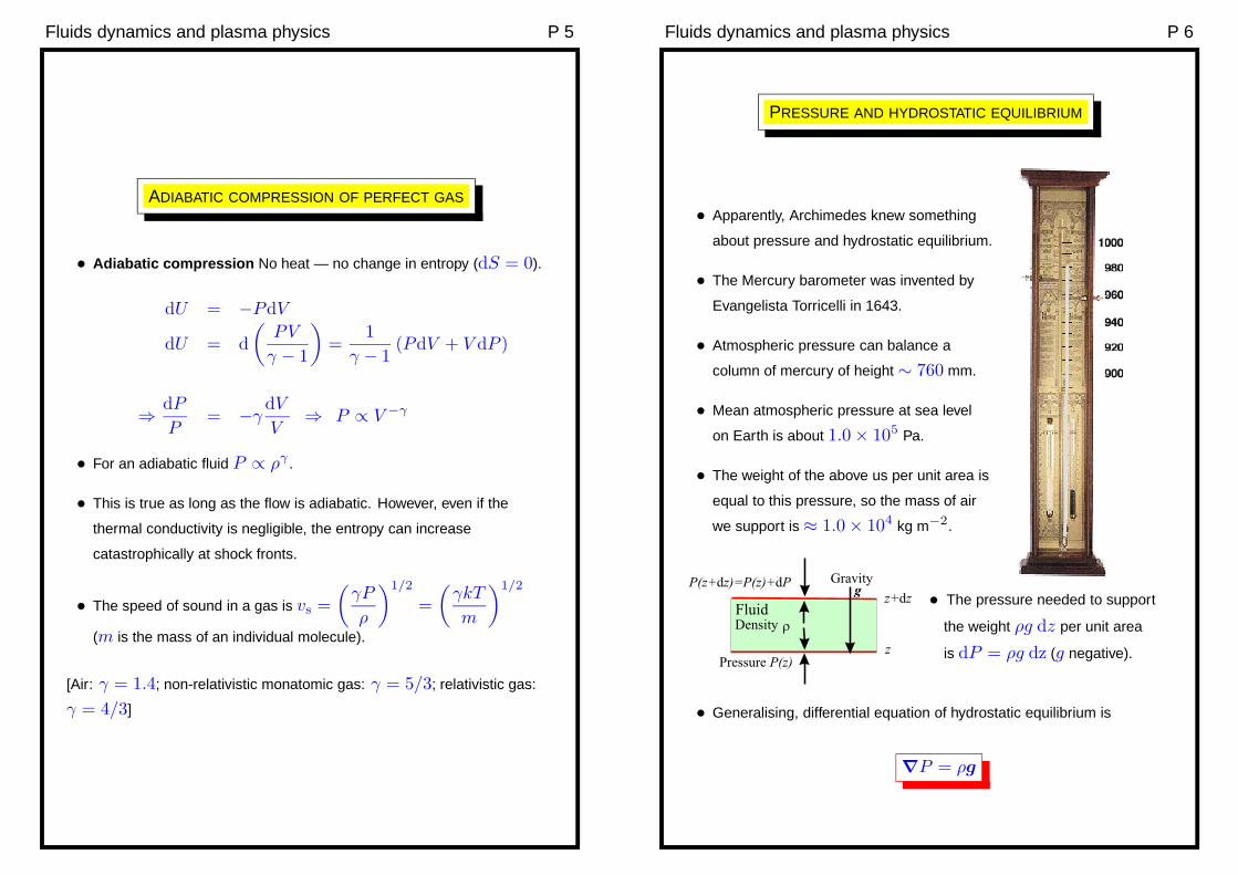
Fluids dynamics and plasma physics P 5
ADIABATIC COMPRESSION OF PERFECT GAS
• Adiabatic compression No heat — no change in entropy (dS = 0).
dU = −PdV
dU = d
(
PV
γ − 1
)
=1
γ − 1(PdV + V dP )
⇒ dP
P= −γ
dV
V⇒ P ∝ V −γ
• For an adiabatic fluid P ∝ ργ .
• This is true as long as the flow is adiabatic. However, even if the
thermal conductivity is negligible, the entropy can increase
catastrophically at shock fronts.
• The speed of sound in a gas is vs =
(
γP
ρ
)1/2
=
(
γkT
m
)1/2
(m is the mass of an individual molecule).
[Air: γ = 1.4; non-relativistic monatomic gas: γ = 5/3; relativistic gas:
γ = 4/3]
Fluids dynamics and plasma physics P 6
PRESSURE AND HYDROSTATIC EQUILIBRIUM
• Apparently, Archimedes knew something
about pressure and hydrostatic equilibrium.
• The Mercury barometer was invented by
Evangelista Torricelli in 1643.
• Atmospheric pressure can balance a
column of mercury of height ∼ 760 mm.
• Mean atmospheric pressure at sea level
on Earth is about 1.0 × 10⁵ Pa.
• The weight of the above us per unit area is
equal to this pressure, so the mass of air
we support is ≈ 1.0 × 10⁴ kg m−2.
• The pressure needed to support
the weight ρg dz per unit area
is dP = ρg dz (g negative).
• Generalising, differential equation of hydrostatic equilibrium is
∇P = ρg

Fluids dynamics and plasma physics P 7
HOT GAS IN CLUSTERS OF GALAXIES
• Abell 2029 is a dynamically relaxed cluster of galaxies at z = 0.0779
(300 Mpc). It contains some active galaxies, but none that disturb the
hot cluster gas very much. It is seen here in X-rays emitted by gas that
fell into the potential well. The spatial extent is about 300 kpc
• The temperature of the gas drops from 9 keV (almost exactly 108 K) in
the outer regions to 4 × 10⁷ K in the centre, where there is a massive
elliptical galaxy that is eating everything that comes close.
• The density of the gas is about 104 particles m−3and spectroscopy
shows that the gas near the centre has been enriched in metals
(metals are anything with Z > 2) due to supernovae.
Fluids dynamics and plasma physics P 8
FLUID DYNAMICS
• When the mean free path λ of particles in a gas or plasma is small
compared to the scales of interest, we can treat the system as a
hydrodynamical fluid.
• We imagine the fluid composed of fluid elements, which are regions
bigger than λ, large enough to have well-defined values of macroscopic
properties; density ρ(x, t), velocity v(x, t); pressure P (x, t); energy
density u(x, t) and anything else that is relevant, e.g. magnetic field.
• A fluid element is acted on by gravity (and other body forces), by
pressure forces and other stresses on the surface.
• These fluid elements stay more or less well-defined (on scales λ),
but the surface of an element is moving at the local fluid velocity, so
elements distort as they move around. The distortions can become
very large — in the presence of turbulent motions the fluid elements
can be dispersed
• There are still some microscopic physical processes occurring on
scales of λ that determine important properties of a fluid: heat
conduction; viscosity. These are transport processes resulting from
interpenetration of the of the velocity distributions from nearby points.
The macroscopic properties can also change discontinuously on scale
so λ at shock fronts.
• We generalise the equation of hydrostatics: 0 = −∇P + ρg to
include the acceleration of a fluid element:
ρDv
Dt= −∇P + ρg
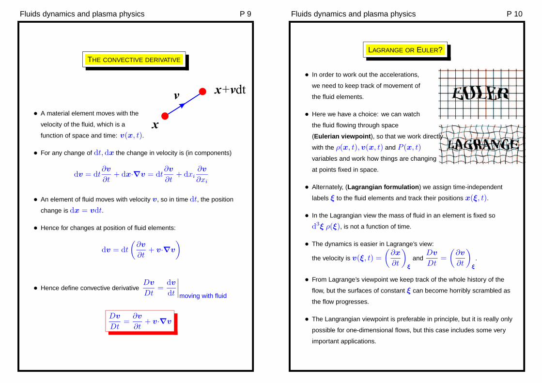
Fluids dynamics and plasma physics P 9
THE CONVECTIVE DERIVATIVE
• A material element moves with the
velocity of the fluid, which is a
function of space and time: v(x, t).
• For any change of dt, dx the change in velocity is (in components)
dv = dt∂v
∂t+ dx·∇v = dt
∂v
∂t+ dxi
∂v
∂xi
• An element of fluid moves with velocity v, so in time dt, the position
change is dx = vdt.
• Hence for changes at position of fluid elements:
dv = dt
(
∂v
∂t+ v·∇v
)
• Hence define convective derivativeDv
Dt=
dv
dt
∣
∣
∣
∣
moving with fluid
Dv
Dt=
∂v
∂t+ v·∇v
Fluids dynamics and plasma physics P 10
LAGRANGE OR EULER?
• In order to work out the accelerations,
we need to keep track of movement of
the fluid elements.
• Here we have a choice: we can watch
the fluid flowing through space
(Eulerian viewpoint), so that we work directly
with the ρ(x, t), v(x, t) and P (x, t)
variables and work how things are changing
at points fixed in space.
• Alternately, (Lagrangian formulation) we assign time-independent
labels ξ to the fluid elements and track their positions x(ξ, t).
• In the Lagrangian view the mass of fluid in an element is fixed so
d3ξ ρ(ξ), is not a function of time.
• The dynamics is easier in Lagrange’s view:
the velocity is v(ξ, t) =
(
∂x
∂t
)
ξ
andDv
Dt=
(
∂v
∂t
)
ξ
.
• From Lagrange’s viewpoint we keep track of the whole history of the
flow, but the surfaces of constant ξ can become horribly scrambled as
the flow progresses.
• The Langrangian viewpoint is preferable in principle, but it is really only
possible for one-dimensional flows, but this case includes some very
important applications.
Fluids dynamics and plasma physics P 11
THE EQUATIONS OF HYDRODYNAMICS
• The equation of continuity is only needed in the Eulerian formulation:
∂ρ
∂t+ ∇·(ρv) = 0
• The Lagrangian force equation (can divide by ρ(x)):
Dv
Dt=
(
∂v
∂t
)
ξ
= − 1
ρ(x)∇P (x) + g(x)
The Eulerian force equation:
ρDv
Dt= ρ
∂v
∂t+ ρv·∇v = −∇P + ρg
• We also need an energy equation: for Lagrangian hydrodynamics we
can use dU = TdS − PdV . For adiabatic flow we can often get
away with using P ∝ ργ . The energy equation in Eulerian form is
complicated by the fact that the volume of fluid elements is changing.
The following equation is only given for completeness (ε is the heat
input per unit volume):
Du
Dt= ε + (Ts − u − P )∇·v
• To make a realistic model of any fluid we also need to consider the
effects of viscosity, and thermal conduction, and the any anisotropic
component to the pressure of a plasma arising from any magnetic field
present.
Fluids dynamics and plasma physics P 12
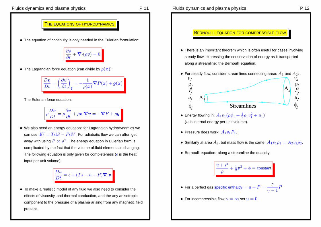
BERNOULLI EQUATION FOR COMPRESSIBLE FLOW
• There is an important theorem which is often useful for cases involving
steady flow, expressing the conservation of energy as it transported
along a streamline: the Bernoulli equation.
• For steady flow, consider streamlines connecting areas A1 and A2:
• Energy flowing in: A1v1(ρφ1 + 12ρ1v
21 + u1)
(u is internal energy per unit volume).
• Pressure does work: A1v1P1.
• Similarly at area A2, but mass flow is the same: A1v1ρ1 = A2v2ρ2.
• Bernoulli equation: along a streamline the quantity
u + P
ρ+ 1
2v2 + φ = constant
• For a perfect gas specific enthalpy = u + P =γ
γ − 1P
• For incompressible flow γ = ∞ set u = 0.
Fluids dynamics and plasma physics P 13
APPROXIMATIONS TO HYDRODYNAMICS
• The equations of compressible hydrodynamics (already a massive
simplification of the microscopic picture) are clearly very complicated.
• They are also notoriously difficult to integrate numerically — in 3-D
computing time scales like (grid size)4. Accuracy also a problem due to
advection through grid, which will blur density contrasts.
• Very useful approximations that yield insight:
- Incompressible flow: ∇·v = 0. Clearly a good model for liquids,
but also a surprisingly good approximation for gases provided the
flow is subsonic.
- Irrotational flow: this is the case when there is no vorticity
∇×××××v = 0. The vorticity field Ω ≡ ∇×××××v moves with the fluid, and
vorticity is usually generated at boundaries, so often the bulk of a
flow is irrotational.
If ∇×××××v = 0 the velocity field can be generated from a scalar potential
v = ∇Φ (sorry, but fluid dynamics has a plus sign here. . . ). If the
fluid is both incompressible and irrotational, the velocity potential
satisfies Laplace’s equation ∇2Φ = 0.
• In this important case a we can use potential theory to find v and
Bernoulli’s theorem to find the pressure.
aFeynman calls it the “flow of dry water” (Lectures: Volume 2)
Fluids dynamics and plasma physics P 14
HYDROSTATIC EQUILIBRIUM OF THE SUN
• The equation of hydrostatic equilibrium for a spherically-symmetric
body of radius R and mass M :
dP (r)
dr= −Gm(r)ρ(r)
r2
where m(r) is the mass interior to r.
• Multiply by 4πr3 and integrate:
[
4πr3P (r)]R
0−3
∫ R
0
dr 4πr2P (r) = −∫ R
0
dr 4πr2ρ(r)Gm(r)
r
• The integrated part is zero if the pressure falls to zero at r = R, and
the integral on the LHS is −3 times the integral of the pressure over
the volume. The RHS is the stored gravitational potential energy, i.e.
the total energy needed to disassemble the sphere.
• The volume-averaged pressure is therefore 〈P 〉 = −Egrav
3V
• The gravitational stored energy depends on the density distribution
Egrav = −fGM2
R, where f is of order unity. For a uniform sphere
f = 3/5, but it would be greater if the density increases towards the
centre.
• For M = 2 × 1030 kg and R = 7 × 10⁸ m, we find a stored energy
of 4 × 1041 J and an average pressure of 〈P 〉 = 9 × 10¹³ Pa
• Assuming that the Sun is made of hydrogen, we calculate that it
contains ≈ 1057 protons and the same number of electrons. Using
PV = NkT we estimate the temperature as ≈ 5 × 10⁶ K, three
orders of magnitude greater than its surface temperature (6000 K)
Fluids dynamics and plasma physics P 15
THE SUN AND BERNOULLI’S THEOREM
• We have concluded that the Sun’s surface is very cool compared to its
interior (the central temperature is 1.56 × 10⁷ K).
• We can get many insights into solar physics by applying Bernoulli’s
theorem to (hypothetical) streamlines connecting the Sun’s surface to
infinity.
• In Bernoulli’s theoremu + P
ρ+ 1
2v2 + φ = constant set
v∞ = 0, P∞ = u∞ = 0, so the constant is zero. Then at the
surface:
- if the material is cold (P = u = 0) we conclude the velocity
(inwards or outwards) is 600 km s−1.
- alternatively, if the velocity is low, the temperature must be
(approximately)
P
ρ=
kT
m=
γ − 1
γ
GM
R⇒ T = 5 × 10⁶ K
• In fact, both alternatives happen: in quiescent conditions there is a hot
solar corona, which produces a slow solar wind 400 km s−1 by heat
conduction to radius of about 2 R.
• In solar flares and coronal ejections, hot material is thrown upwards,
where it escapes as a faster solar wind at ≈ 700 km s−1.
Fluids dynamics and plasma physics P 16
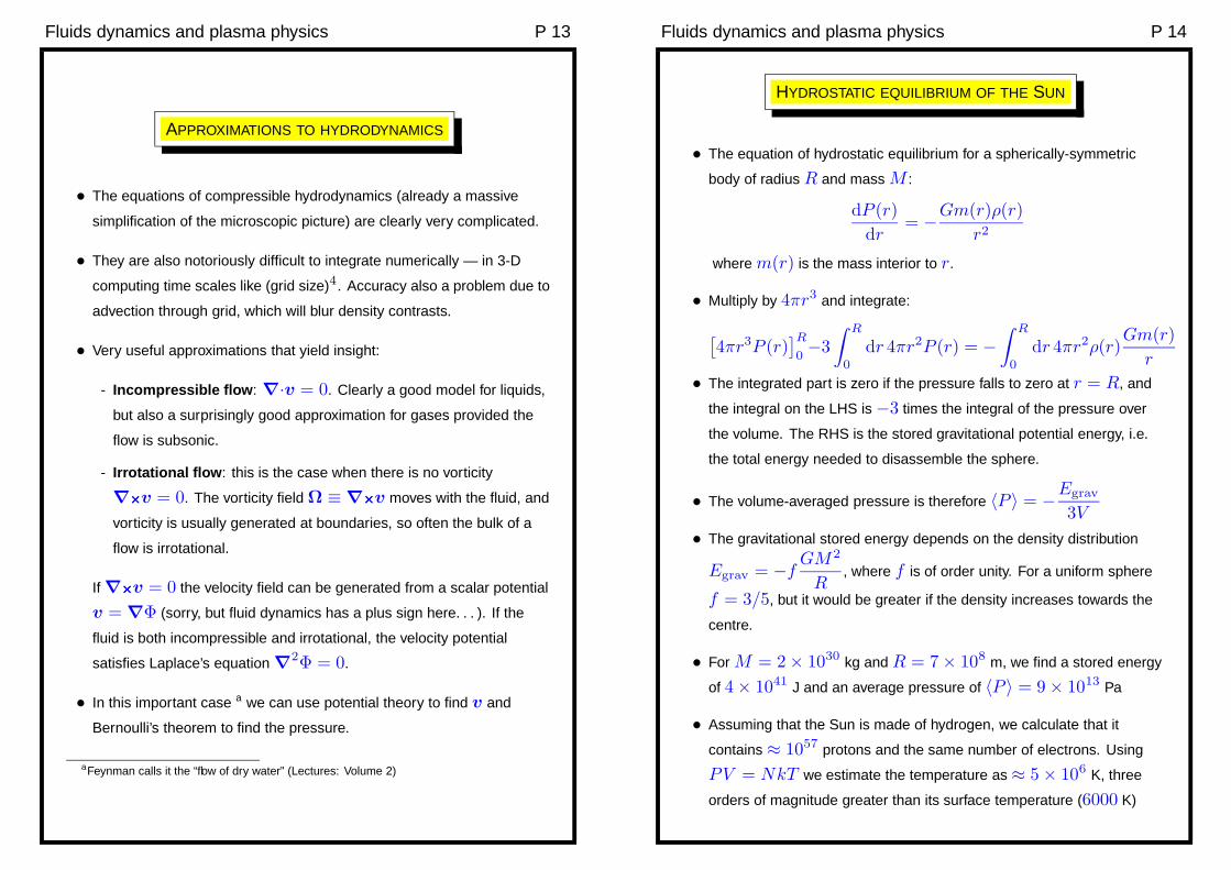
BERNOULLI EQUATION FOR INCOMPRESSIBLE FLOW
• Flow from water tank or bathtub.
• The pressure is the same at the top of
the tank at point A where v = 0 and at
point B where the water escapes.
• Use Bernoulli:
P + 12v2 + gh = constant.
• This says the outflow velocity is√
2gh.
• The actual draining rate might not be equal to this velocity times the
area of the hole, since the flow can still be converging as the water
leaves the tank.
• Efflux coefficient (effective area of hole divided by geometric area)
varies between 0.5 to 1. For a simple hole in the side of a
tank it is 0.62.
• Cylindrical jet hitting a wall
• Ignore gravity for this problem.
• The stagnation point at A must have
pressure P0 + 12ρv2
0 .
• The pressure at B (large radius
compared to jet radius) must be
P0 again, so Bernoulli says that the velocity is v0 there.
Fluids dynamics and plasma physics P 17
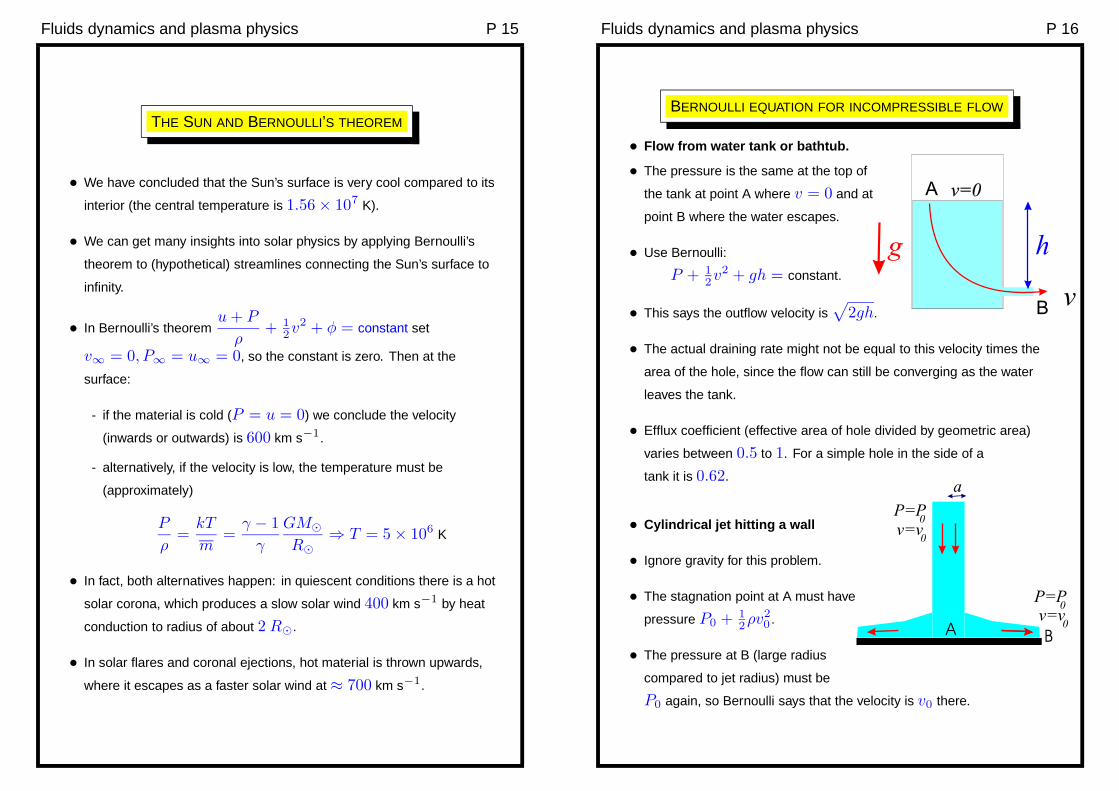
COLLISIONAL PROCESSES: VISCOSITY AND THERMAL CONDUCTIVITY
• Viscosity and thermal conductivity in fluids and plasmas are
determined by the extent to which the particle distributions at different
spatial position can interpenetrate; i.e. it depends on the mean free
path λ.
• For collisional fluids this is related to the thermal velocity vT and
collision frequency νc by λ ≈ vT
νc
.
• Consider the transport of a quantity Q
which varies macroscopically with
position.
• Q might be the specific energy u
(thermal conductivity) or a component
of the momentum ρv (viscosity).
• Transport of a Q then occurs by exchange
of “blobs” of amount ∆Q, travelling a distance λ at velocity vT .
• This random walk leads to a diffusion equation for property Q, in the
frame moving with the fluid element:
13λvT∇
2Q =DQ
Dt
• The factor of 13
in the diffusion coefficient accounts for the fact that the
blob is free to move in any of the three dimensions.
Fluids dynamics and plasma physics P 18
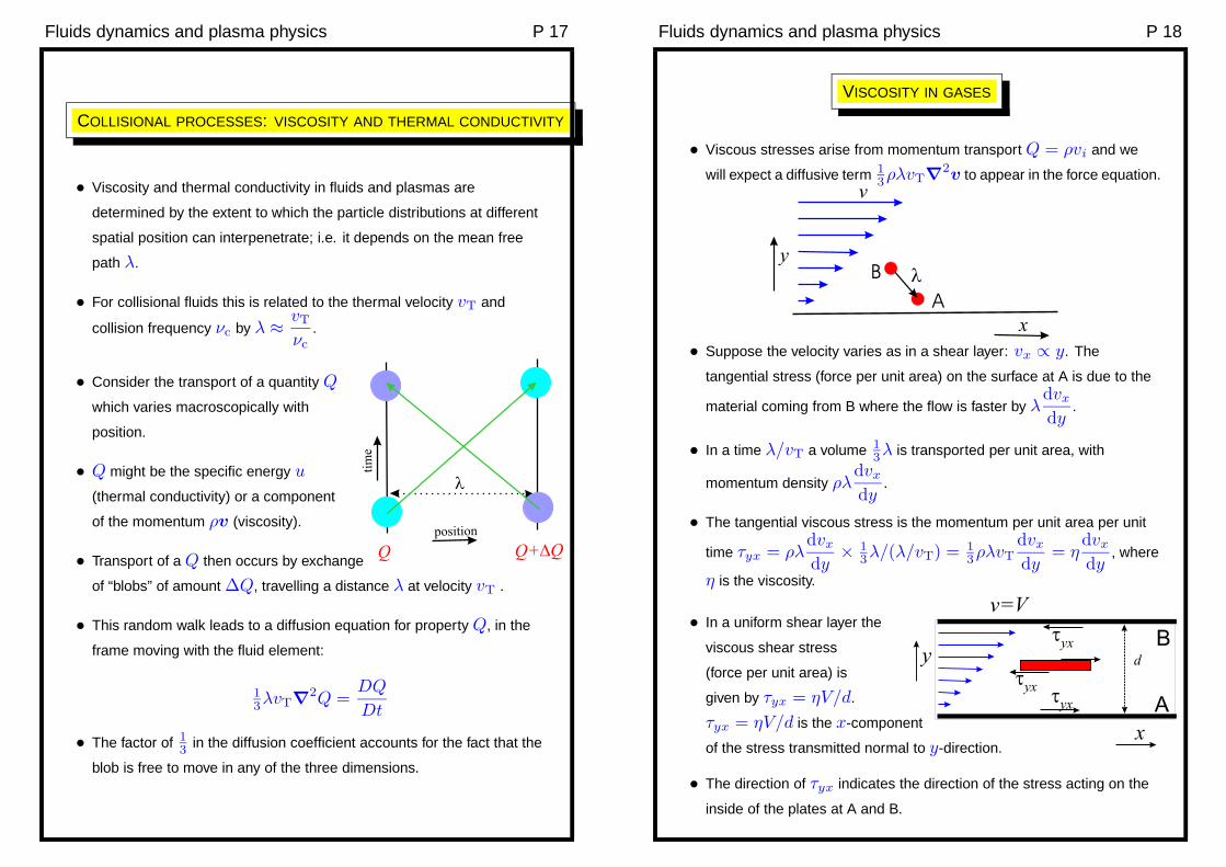
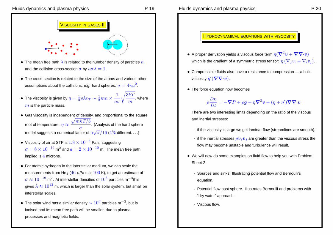
VISCOSITY IN GASES
• Viscous stresses arise from momentum transport Q = ρvi and we
will expect a diffusive term 13ρλvT∇
2v to appear in the force equation.
• Suppose the velocity varies as in a shear layer: vx ∝ y. The
tangential stress (force per unit area) on the surface at A is due to the
material coming from B where the flow is faster by λdvx
dy.
• In a time λ/vT a volume 13λ is transported per unit area, with
momentum density ρλdvx
dy.
• The tangential viscous stress is the momentum per unit area per unit
time τyx = ρλdvx
dy× 1
3λ/(λ/vT) = 1
3ρλvT
dvx
dy= η
dvx
dy, where
η is the viscosity.
x
dytyx
tyx
tyx A
B
v=V• In a uniform shear layer the
viscous shear stress
(force per unit area) is
given by τyx = ηV/d.
τyx = ηV/d is the x-component
of the stress transmitted normal to y-direction.
• The direction of τyx indicates the direction of the stress acting on the
inside of the plates at A and B.
Fluids dynamics and plasma physics P 19
VISCOSITY IN GASES II
• The mean free path λ is related to the number density of particles n
and the collision cross-section σ by nσλ = 1.
• The cross-section is related to the size of the atoms and various other
assumptions about the collisions, e.g. hard spheres: σ = 4πa2.
• The viscosity is given by η = 13ρλvT ∼ 1
3mn × 1
nσ
√
3kT
m, where
m is the particle mass.
• Gas viscosity is independent of density, and proportional to the square
root of temperature: η ≈√
mkT/3
σ. (Analysis of the hard sphere
model suggests a numerical factor of 5√
π/16 (4% different. . . .)
• Viscosity of air at STP is 1.8 × 10⁻⁵ Pa s, suggesting
σ = 8 × 10⁻¹⁹ m2 and a = 2 × 10⁻¹⁰ m. The mean free path
implied is 4 microns.
• For atomic hydrogen in the interstellar medium, we can scale the
measurements from He4 (46 µPa s at 100 K), to get an estimate of
σ ≈ 10−19 m2. At interstellar densities of 106 particles m−3this
gives λ ≈ 1013 m, which is larger than the solar system, but small on
interstellar scales.
• The solar wind has a similar density ∼ 106 particles m−3, but is
ionised and its mean free path will be smaller, due to plasma
processes and magnetic fields.
Fluids dynamics and plasma physics P 20
HYDRODYNAMICAL EQUATIONS WITH VISCOSITY
• A proper derivation yields a viscous force term η(∇2v + ∇∇·v)
which is the gradient of a symmetric stress tensor: η (∇jvi + ∇ivj).
• Compressible fluids also have a resistance to compression — a bulk
viscosity η′(∇∇·v).
• The force equation now becomes
ρDv
Dt= −∇P + ρg + η∇
2v + (η + η′)∇∇·v
There are two interesting limits depending on the ratio of the viscous
and inertial stresses:
- if the viscosity is large we get laminar flow (streamlines are smooth).
- if the inertial stresses ρvivj are greater than the viscous stress the
flow may become unstable and turbulence will result.
• We will now do some examples on fluid flow to help you with Problem
Sheet 2.
- Sources and sinks. Illustrating potential flow and Bernoulli’s
equation.
- Potential flow past sphere. Illustrates Bernoulli and problems with
“dry water” approach.
- Viscous flow.
Fluids dynamics and plasma physics P 21
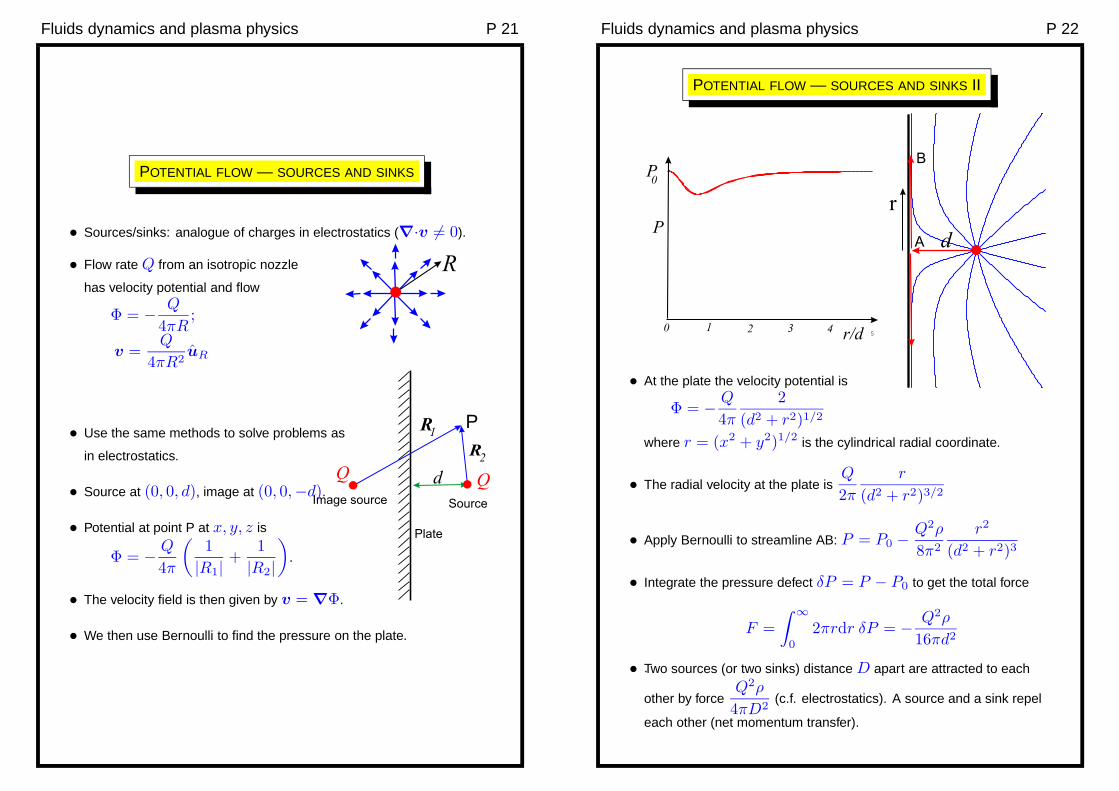
POTENTIAL FLOW — SOURCES AND SINKS
• Sources/sinks: analogue of charges in electrostatics (∇·v 6= 0).
• Flow rate Q from an isotropic nozzle
has velocity potential and flow
Φ = − Q
4πR;
v =Q
4πR2uR
• Use the same methods to solve problems as
in electrostatics.
• Source at (0, 0, d), image at (0, 0,−d).
• Potential at point P at x, y, z is
Φ = − Q
4π
(
1
|R1|+
1
|R2|
)
.
• The velocity field is then given by v = ∇Φ.
• We then use Bernoulli to find the pressure on the plate.
Fluids dynamics and plasma physics P 22
POTENTIAL FLOW — SOURCES AND SINKS II
• At the plate the velocity potential is
Φ = − Q
4π
2
(d2 + r2)1/2
where r = (x2 + y2)1/2 is the cylindrical radial coordinate.
• The radial velocity at the plate isQ
2π
r
(d2 + r2)3/2
• Apply Bernoulli to streamline AB: P = P0 −Q2ρ
8π2
r2
(d2 + r2)3
• Integrate the pressure defect δP = P − P0 to get the total force
F =
∫ ∞
0
2πrdr δP = − Q2ρ
16πd2
.• Two sources (or two sinks) distance D apart are attracted to each
other by forceQ2ρ
4πD2(c.f. electrostatics). A source and a sink repel
each other (net momentum transfer).
Fluids dynamics and plasma physics P 23
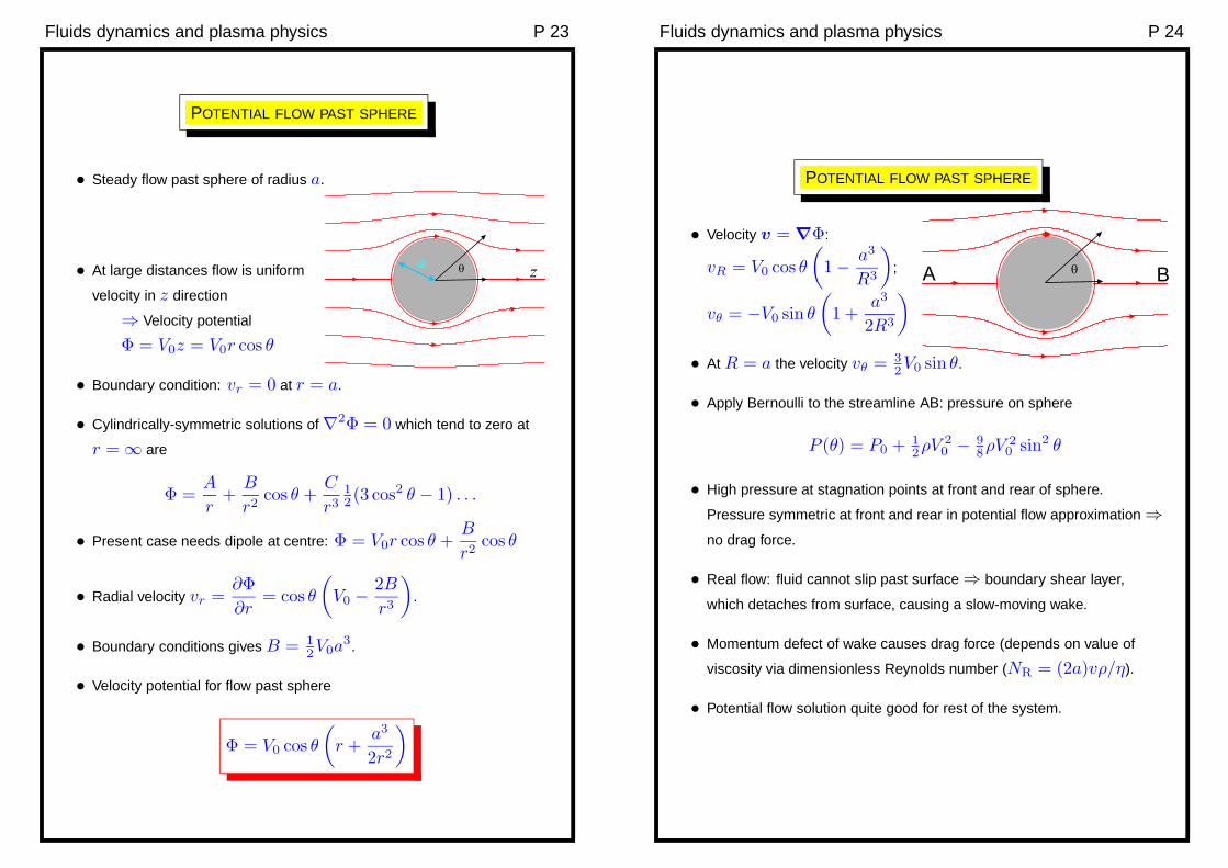
POTENTIAL FLOW PAST SPHERE
• Steady flow past sphere of radius a.
• At large distances flow is uniform
velocity in z direction
⇒ Velocity potential
Φ = V0z = V0r cos θ
• Boundary condition: vr = 0 at r = a.
• Cylindrically-symmetric solutions of ∇2Φ = 0 which tend to zero at
r = ∞ are
Φ =A
r+
B
r2cos θ +
C
r312(3 cos2 θ − 1) . . .
• Present case needs dipole at centre: Φ = V0r cos θ +B
r2cos θ
• Radial velocity vr =∂Φ
∂r= cos θ
(
V0 −2B
r3
)
.
• Boundary conditions gives B = 12V0a
3.
• Velocity potential for flow past sphere
Φ = V0 cos θ
(
r +a3
2r2
)
Fluids dynamics and plasma physics P 24
POTENTIAL FLOW PAST SPHERE
• Velocity v = ∇Φ:
vR = V0 cos θ
(
1 − a3
R3
)
;
vθ = −V0 sin θ
(
1 +a3
2R3
)
• At R = a the velocity vθ = 32V0 sin θ.
• Apply Bernoulli to the streamline AB: pressure on sphere
P (θ) = P0 + 12ρV 2
0 − 98ρV 2
0 sin2 θ
• High pressure at stagnation points at front and rear of sphere.
Pressure symmetric at front and rear in potential flow approximation ⇒no drag force.
• Real flow: fluid cannot slip past surface ⇒ boundary shear layer,
which detaches from surface, causing a slow-moving wake.
• Momentum defect of wake causes drag force (depends on value of
viscosity via dimensionless Reynolds number (NR = (2a)vρ/η).
• Potential flow solution quite good for rest of the system.
Fluids dynamics and plasma physics P 25
BOUNDARY LAYERS
Boundary layer
v
v=0
d
• Boundary condition for surface
of solid body: no radial or tangential
velocity (no slip).
• Flow past a solid body must develop
a boundary layer with a velocity
gradient. This is a region with vorticity (∇×××××v 6= 0), which can then
enter the fluid flow.
• The ratio of the inertial stress ρv2 to the viscous stress ηv/L is an
important dimensionless quantity known as the Reynolds number
NR =ρvL
η.
• If the inertial stress is too high in a flow random transverse motions will
cause turbulent mixing, which in turn increases the effective “eddy
viscosity”
(
η
ρ
)
effective
∼ veddyLeddy.
• Turbulence transports energy to smaller scales (and to larger scales)
by splitting up of eddies on a timescale Leddy/veddy.
• Energy is rapidly transported to the smallest scales, where viscous
dissipation can occur.
Fluids dynamics and plasma physics P 26
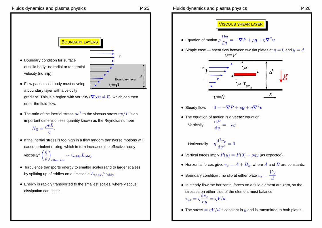
VISCOUS SHEAR LAYER
• Equation of motion ρDv
Dt= −∇P + ρg + η∇
2v
• Simple case — shear flow between two flat plates at y = 0 and y = d.
x
d
v=V
y
tyxtyx
tyx
g
v=0
• Steady flow: 0 = −∇P + ρg + η∇2v
• The equation of motion is a vector equation:
VerticallydP
dy= −ρg
Horizontally ηd2vx
dy2= 0
• Vertical forces imply P (y) = P (0) − ρgy (as expected).
• Horizontal forces give: vx = A + By, where A and B are constants.
• Boundary condition : no slip at either plate vx =V y
d
• In steady flow the horizontal forces on a fluid element are zero, so the
stresses on either side of the element must balance:
τyx = ηdvx
dy= ηV/d.
• The stress = ηV/d is constant in y and is transmitted to both plates.
Fluids dynamics and plasma physics P 27
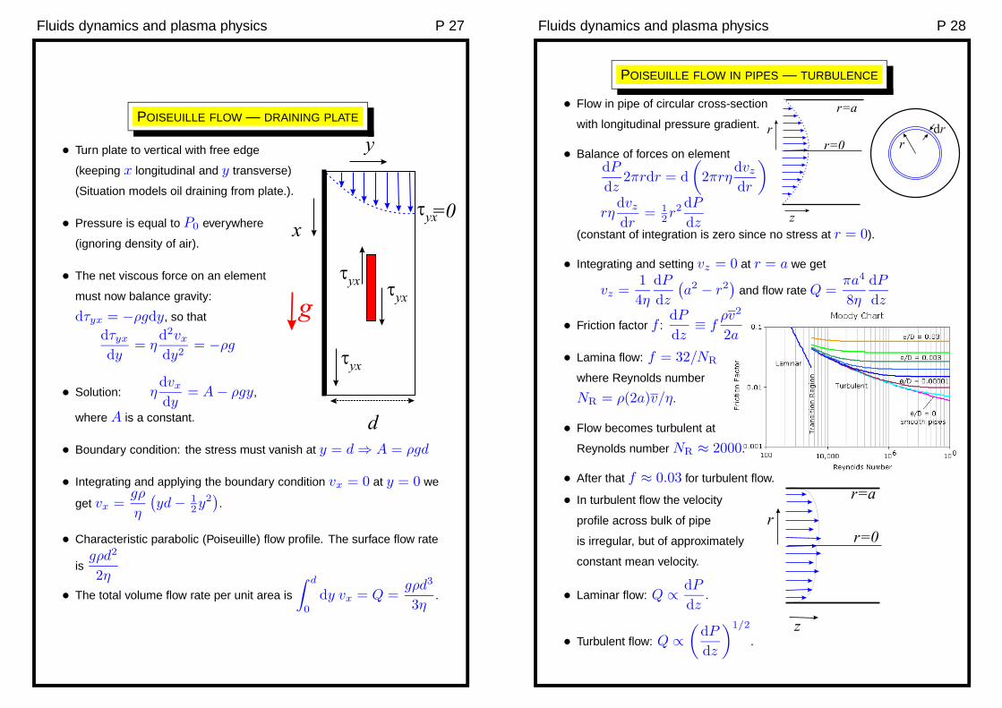
POISEUILLE FLOW — DRAINING PLATE
• Turn plate to vertical with free edge
(keeping x longitudinal and y transverse)
(Situation models oil draining from plate.).
• Pressure is equal to P0 everywhere
(ignoring density of air).
• The net viscous force on an element
must now balance gravity:
dτyx = −ρgdy, so that
dτyx
dy= η
d2vx
dy2= −ρg
• Solution: ηdvx
dy= A − ρgy,
where A is a constant.
• Boundary condition: the stress must vanish at y = d ⇒ A = ρgd
• Integrating and applying the boundary condition vx = 0 at y = 0 we
get vx =gρ
η
(
yd − 12y2
)
.
• Characteristic parabolic (Poiseuille) flow profile. The surface flow rate
isgρd2
2η
• The total volume flow rate per unit area is
∫ d
0
dy vx = Q =gρd3
3η.
Fluids dynamics and plasma physics P 28
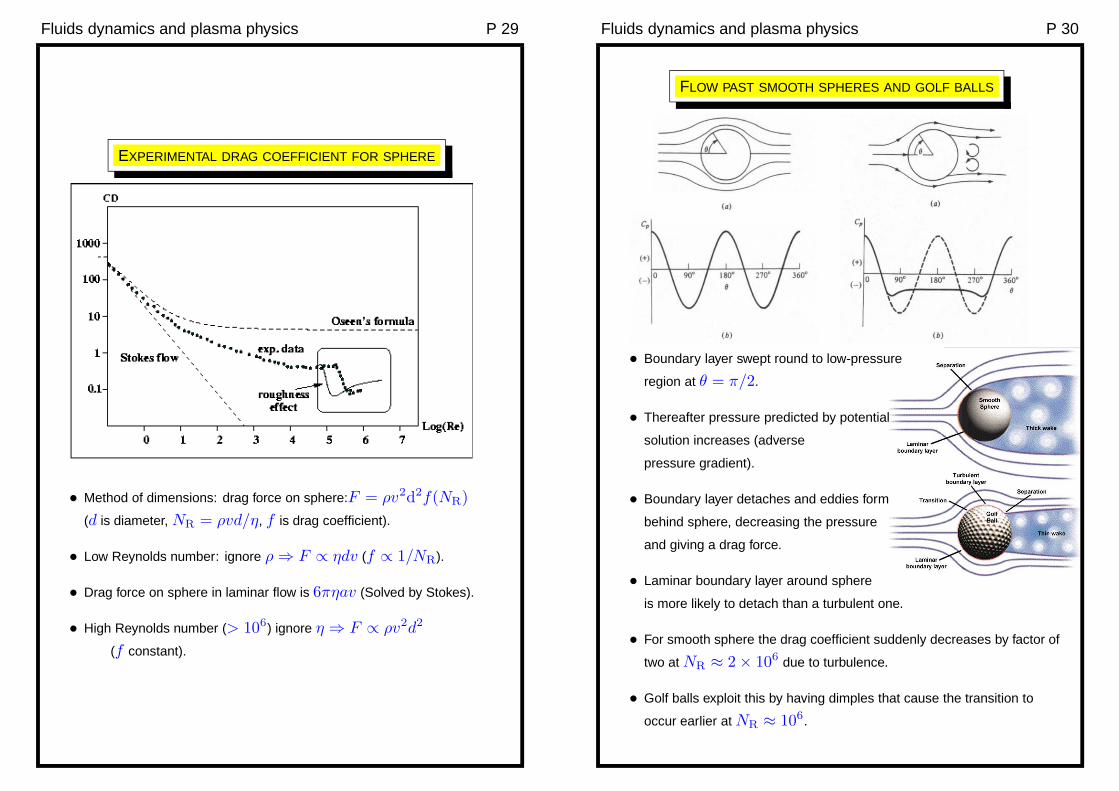
POISEUILLE FLOW IN PIPES — TURBULENCE
• Flow in pipe of circular cross-section
with longitudinal pressure gradient.
• Balance of forces on elementdP
dz2πrdr = d
(
2πrηdvz
dr
)
rηdvz
dr= 1
2r2 dP
dz(constant of integration is zero since no stress at r = 0).
• Integrating and setting vz = 0 at r = a we get
vz =1
4η
dP
dz
(
a2 − r2)
and flow rate Q =πa4
8η
dP
dz
• Friction factor f :dP
dz≡ f
ρv2
2a
• Lamina flow: f = 32/NR
where Reynolds number
NR = ρ(2a)v/η.
• Flow becomes turbulent at
Reynolds number NR ≈ 2000.
• After that f ≈ 0.03 for turbulent flow.
• In turbulent flow the velocity
profile across bulk of pipe
is irregular, but of approximately
constant mean velocity.
• Laminar flow: Q ∝ dP
dz.
• Turbulent flow: Q ∝(
dP
dz
)1/2
.
Fluids dynamics and plasma physics P 29
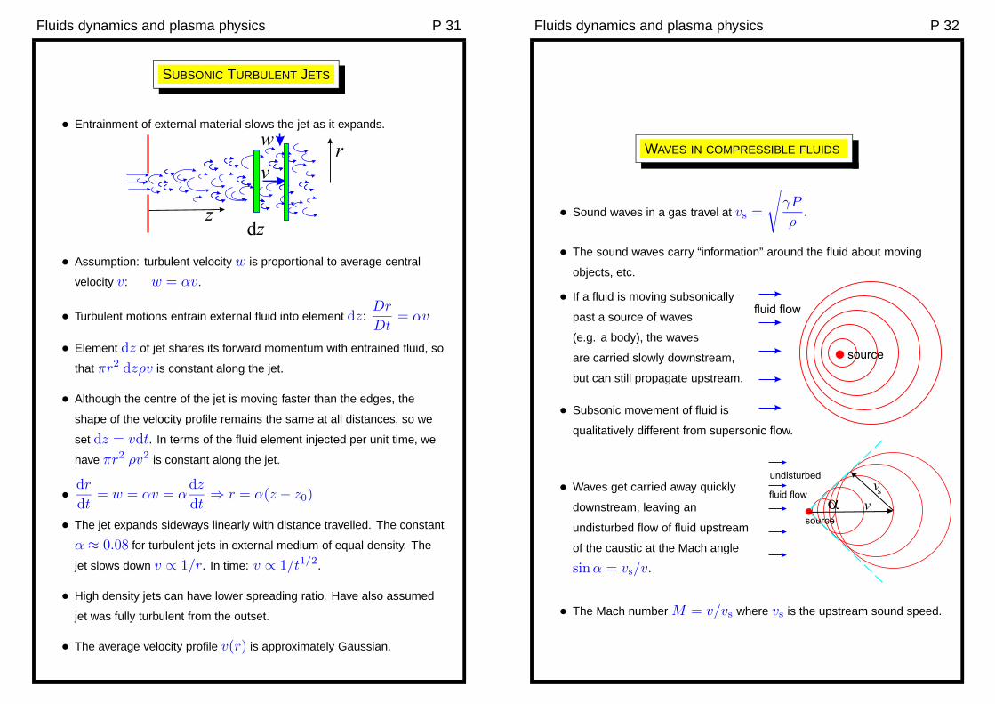
EXPERIMENTAL DRAG COEFFICIENT FOR SPHERE
• Method of dimensions: drag force on sphere:F = ρv2d2f(NR)
(d is diameter, NR = ρvd/η, f is drag coefficient).
• Low Reynolds number: ignore ρ ⇒ F ∝ ηdv (f ∝ 1/NR).
• Drag force on sphere in laminar flow is 6πηav (Solved by Stokes).
• High Reynolds number (> 106) ignore η ⇒ F ∝ ρv2d2
(f constant).
Fluids dynamics and plasma physics P 30
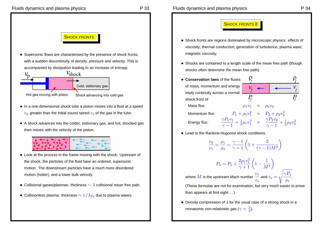
FLOW PAST SMOOTH SPHERES AND GOLF BALLS
• Boundary layer swept round to low-pressure
region at θ = π/2.
• Thereafter pressure predicted by potential
solution increases (adverse
pressure gradient).
• Boundary layer detaches and eddies form
behind sphere, decreasing the pressure
and giving a drag force.
• Laminar boundary layer around sphere
is more likely to detach than a turbulent one.
• For smooth sphere the drag coefficient suddenly decreases by factor of
two at NR ≈ 2 × 10⁶ due to turbulence.
• Golf balls exploit this by having dimples that cause the transition to
occur earlier at NR ≈ 106.
Fluids dynamics and plasma physics P 31
SUBSONIC TURBULENT JETS
• Entrainment of external material slows the jet as it expands.
• Assumption: turbulent velocity w is proportional to average central
velocity v: w = αv.
• Turbulent motions entrain external fluid into element dz:Dr
Dt= αv
• Element dz of jet shares its forward momentum with entrained fluid, so
that πr2 dzρv is constant along the jet.
• Although the centre of the jet is moving faster than the edges, the
shape of the velocity profile remains the same at all distances, so we
set dz = vdt. In terms of the fluid element injected per unit time, we
have πr2 ρv2 is constant along the jet.
• dr
dt= w = αv = α
dz
dt⇒ r = α(z − z0)
• The jet expands sideways linearly with distance travelled. The constant
α ≈ 0.08 for turbulent jets in external medium of equal density. The
jet slows down v ∝ 1/r. In time: v ∝ 1/t1/2.
• High density jets can have lower spreading ratio. Have also assumed
jet was fully turbulent from the outset.
• The average velocity profile v(r) is approximately Gaussian.
Fluids dynamics and plasma physics P 32
WAVES IN COMPRESSIBLE FLUIDS
• Sound waves in a gas travel at vs =
√
γP
ρ.
• The sound waves carry “information” around the fluid about moving
objects, etc.
• If a fluid is moving subsonically
past a source of waves
(e.g. a body), the waves
are carried slowly downstream,
but can still propagate upstream.
• Subsonic movement of fluid is
qualitatively different from supersonic flow.
• The Mach number M = v/vs where vs is the upstream sound speed.
• Waves get carried away quickly
downstream, leaving an
undisturbed flow of fluid upstream
of the caustic at the Mach angle
sinα = vs/v.
Fluids dynamics and plasma physics P 33
SHOCK FRONTS
• Supersonic flows are characterised by the presence of shock fronts,
with a sudden discontinuity of density, pressure and velocity. This is
accompanied by dissipation leading to an increase of entropy.
• In a one-dimensional shock tube a piston moves into a fluid at a speed
vp greater than the initial sound speed vs of the gas in the tube.
• A shock advances into the colder, stationary gas, and hot, shocked gas
then moves with the velocity of the piston.
• Look at the process in the frame moving with the shock. Upstream of
the shock, the particles of the fluid have an ordered, supersonic
motion. The downstream particles have a much more disordered
motion (hotter), and a lower bulk velocity.
• Collisional gases/plasmas: thickness ∼ λ collisional mean free path.
• Collisionless plasma: thickness ∼ v/λDi due to plasma waves.
Fluids dynamics and plasma physics P 34
SHOCK FRONTS II
• Shock fronts are regions dominated by microscopic physics: effects of
viscosity; thermal conduction; generation of turbulence; plasma wave;
magnetic viscosity.
• Shocks are contained to a length scale of the mean free path (though
shocks often determine the mean free path).
• Conservation laws of the fluxes
of mass, momentum and energy
imply continuity across a normal
shock front of
Mass flux: ρ1v1 = ρ2v2
Momentum flux: P1 + ρ1v21 = P2 + ρ2v
22
Energy flux:γP1v1
γ − 1+ 1
2ρ1v
31 =
γP2v2
γ − 1+ 1
2ρ2v
32
• Lead to the Rankine-Hugoniot shock conditions.
v2
v1
=ρ1
ρ2
=γ − 1
γ + 1
(
1 +2
(γ − 1)M2
)
P2 = P1 +2ρ1v
21
γ + 1
(
1 − 1
M2
)
where M is the upstream Mach numberv1
vs
and vs =
√
γP1
ρ1
.
(These formulae are not for examination, but very much easier to prove
than appears at first sight. . . )
• Density compression of 4 for the usual case of a strong shock in a
monatomic non-relativistic gas (γ = 53
).
Fluids dynamics and plasma physics P 35
ASTROPHYSICAL PLASMA PHYSICS
• Plasma is a state of matter containing significant ionisation. Plasma is
very different from other states of matter (solid, liquid, gas). Why?
• A plasma is a soup of oppositely charged particles: electrons/ions (or
e−/e+). These particles interact via strong, long-range
electromagnetic forces. In gases the interparticle forces are short
range and only important in collisions.
• Plasmas show a wide range of new, collective phenomena (plasma
waves). These can interact with each other and the particles,
producing plasma turbulence and particle acceleration.
• Most important is the plasma frequency ωpe =
(
nee2
ε0me
)1/2
. The
whole plasma undergoes longitudinal oscillations at this frequency.
• The extent to which particle behave individually or collectively is
determined by the Debye length — the distance a thermal particle
travels in time 1/ωpe. Electric fields are screened on scales larger
than λDe = vT/ωp =
(
ε0kTe
nee2
)1/2
.
• Influence of magnetic field is hugely important:
- Particles circulate the field lines at the gyro frequency ωge =eB
meThis limits the mobility of individual particles to the Larmor radius,
which is tiny on astrophysical scales. Particles can still stream
along field lines, but will scatter off magnetic irregularities.
- the anisotropic magnetic pressure can be very important
dynamically, particularly near compact objects (stars/neutron stars).
Fluids dynamics and plasma physics P 36
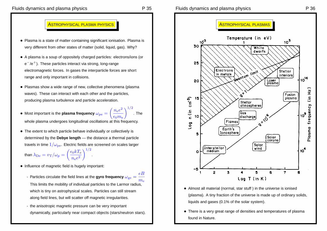
ASTROPHYSICAL PLASMAS
• Almost all material (normal, star stuff ) in the universe is ionised
(plasma). A tiny fraction of the universe is made up of ordinary solids,
liquids and gases (0.1% of the solar system).
• There is a very great range of densities and temperatures of plasma
found in Nature.
Fluids dynamics and plasma physics P 37
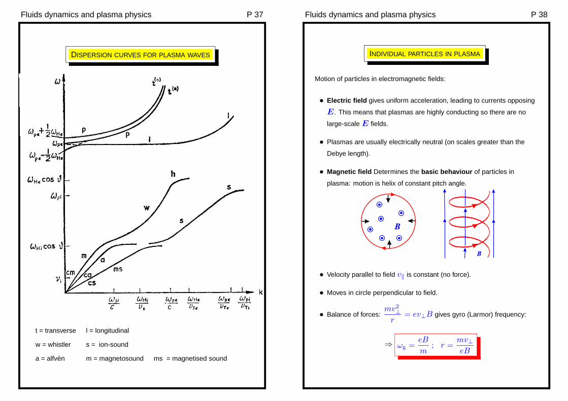
DISPERSION CURVES FOR PLASMA WAVES
t = transverse l = longitudinal
w = whistler s = ion-sound
a = alfven m = magnetosound ms = magnetised sound
Fluids dynamics and plasma physics P 38
INDIVIDUAL PARTICLES IN PLASMA
Motion of particles in electromagnetic fields:
• Electric field gives uniform acceleration, leading to currents opposing
E. This means that plasmas are highly conducting so there are no
large-scale E fields.
• Plasmas are usually electrically neutral (on scales greater than the
Debye length).
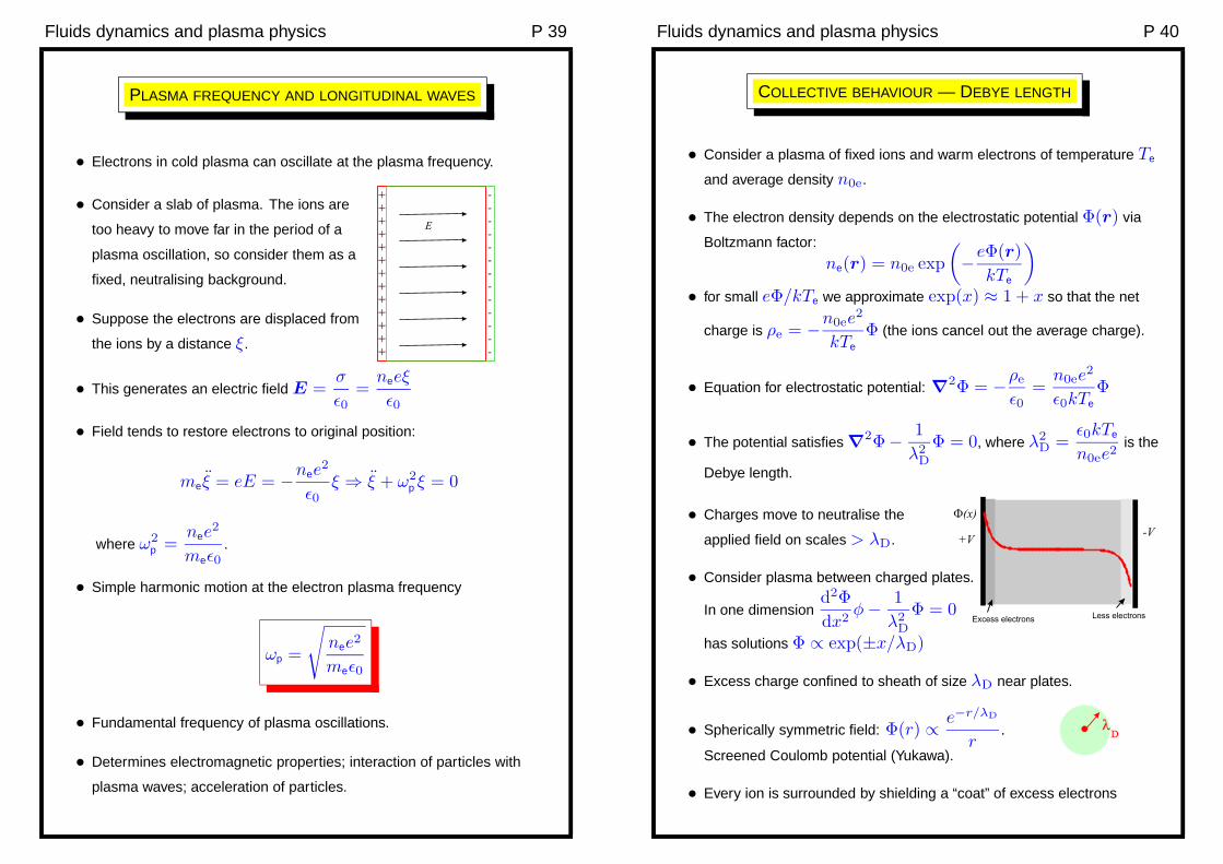
• Magnetic field Determines the basic behaviour of particles in
plasma: motion is helix of constant pitch angle.
• Velocity parallel to field v‖ is constant (no force).
• Moves in circle perpendicular to field.
• Balance of forces:mv2
⊥
r= ev⊥B gives gyro (Larmor) frequency:
⇒ ωg =eB
m; r =
mv⊥eB
Fluids dynamics and plasma physics P 39
PLASMA FREQUENCY AND LONGITUDINAL WAVES
• Electrons in cold plasma can oscillate at the plasma frequency.
• Consider a slab of plasma. The ions are
too heavy to move far in the period of a
plasma oscillation, so consider them as a
fixed, neutralising background.
• Suppose the electrons are displaced from
the ions by a distance ξ.
• This generates an electric field E =σ
ε0=
neeξ
ε0
• Field tends to restore electrons to original position:
meξ = eE = −nee2
ε0ξ ⇒ ξ + ω2
p ξ = 0
where ω2p =
nee2
meε0.
• Simple harmonic motion at the electron plasma frequency
ωp =
√
nee2
meε0
• Fundamental frequency of plasma oscillations.
• Determines electromagnetic properties; interaction of particles with
plasma waves; acceleration of particles.
Fluids dynamics and plasma physics P 40
COLLECTIVE BEHAVIOUR — DEBYE LENGTH
• Consider a plasma of fixed ions and warm electrons of temperature Te
and average density n0e.
• The electron density depends on the electrostatic potential Φ(r) via
Boltzmann factor:
ne(r) = n0e exp
(
−eΦ(r)
kTe
)
• for small eΦ/kTe we approximate exp(x) ≈ 1 + x so that the net
charge is ρe = −n0ee2
kTe
Φ (the ions cancel out the average charge).
• Equation for electrostatic potential: ∇2Φ = −ρe
ε0=
n0ee2
ε0kTe
Φ
• The potential satisfies ∇2Φ− 1
λ2D
Φ = 0, where λ2D =
ε0kTe
n0ee2is the
Debye length.
• Charges move to neutralise the
applied field on scales > λD.
• Consider plasma between charged plates.
In one dimensiond2Φ
dx2φ − 1
λ2D
Φ = 0
has solutions Φ ∝ exp(±x/λD)
• Excess charge confined to sheath of size λD near plates.
• Spherically symmetric field: Φ(r) ∝ e−r/λD
r.
Screened Coulomb potential (Yukawa).
• Every ion is surrounded by shielding a “coat” of excess electrons

Fluids dynamics and plasma physics P 41
DEBYE NUMBER
• Consider a sphere of radius the Debye length λD.
It contains ND ≡ 43πλ3
Dne electrons: the Debye number.
• The Debye number is the number of electrons in the “coat” shielding
any ion in the plasma.
• The Debye number is a measure of the importance of collective effects
in the plasma.
• If ND < 1 there are no collective effects. The “plasma” is merely a
collection of individual particles.
• If ND > 1 it is a true plasma and cooperative effects are important.
• Usually ND 1, with ND ranging from 104 (laboratory) to 1032
(cluster of galaxies).
Fluids dynamics and plasma physics P 42
COLLISIONS IN PLASMA
• Mean free paths in plasma are determined by long-range interactions
between ions and electrons. The collision process is almost exactly the
same as we have seen for gravitational interactions in a galaxy.
• Electron-ion collisions. Consider an electron moving at v going past
a stationary ion with impact parameter b.
• We assume that the interaction is so weak that we can approximate the
trajectory as a straight line, moving at constant velocity.
• Maximum lateral forceZe2
4πε0b2applied for a time ≈ 2b
v
• Momentum transfer per “collision” ∆p =2Ze2
4πε0bv(exact result).
• The lateral momentum changes have
random directions, but the effect
on⟨
∆p2⟩
is cumulative:⟨
∆p2(t)⟩
= ∆p2 × Ncoll.
• Number of collisions with
impact parameter b → b + db
per unit time is 2πb db ni v,
where ni = ne/Z .
Fluids dynamics and plasma physics P 43
MEAN FREE PATHS IN COLLISIONLESS SYSTEMS
• The rate of increase of⟨
∆p2(t)⟩
per unit time is
≈∫
db 2πb niv
(
2Ze2
4πε0bv
)2
= neZe4
2πε20vlog(bmax/bmin)
• The cumulative effects of the
small collisions build up and
are significant when the overall⟨
∆p2⟩
≈ m2v2
• Setting v = v ≈√
kTe/me and expressing everything in terms of ne
and Te we get a mean free path λei = τcollv = v/νei
λei ≈m2v4ε20
neZe4 log Λe
≈ k2T 2e ε20
Znee4 log Λe
=NDλD
Z log Λe
where log Λe = log(bmax/bmin).
• The largest impact parameter is bmax ≈ λD since the ions are
screened beyond this distance.
• The largest amount of momentum that can be transferred is
∆p ≈ mev, so bmin =Ze2me
4πε0v2≈ Ze2me
ε0kT=
Z
neλ2D
.
• The logarithm log Λe is therefore simply log(ND/Z), showing how
all aspects of the collision process involve collective effects.
• νee ≈ νei, but ions are heavier soνii
νee
≈(
Te
Ti
)3/2 (
me
mi
)1/2
Fluids dynamics and plasma physics P 44
PLASMAS AS FLUIDS
• A plasma is a highly conducting fluid. In a stationary medium we have
the constitutive relation (Ohm’s law) j = σE.
• In a (non-relativistic) medium this becomes j = σ(E + v×××××B). If the
medium is highly conducting and we let σ → ∞, so E = −v×××××B.
• Taken together with the induction equation ∇×××××E = −∂B
∂t, this gives
∂B
∂t= ∇××××× (v×××××B)
.• One can show that this means that the magnetic field lines are “frozen
in” and move with the fluid velocity.
• In the force equation of fluid dynamics we have to add a term j×××××B.
For fluid motions we ignore the displacement current and set
∇×××××B = µ0J to get
ρDv
Dt= −∇P + ρg − 1
µ0
(B××××× (∇×××××B))
• We can write
[
1
µ0
(B××××× (∇×××××B))
]
i
= ∇jPmagij where
Pmagij =
(
B2δij
2µ0
− BiBj
µ0
)
(used ∇·B = 0).
• There is an additional anisotropic magnetic pressure, which has a
magnitudeB2
2µ0
. Magnetic field provides a pressure force
perpendicular to the field, but a tension in the direction of the field lines.
• The tension leads to a new form of magnetohydrodynamic wave —
Alfven waves, which are like waves on magnetic strings.
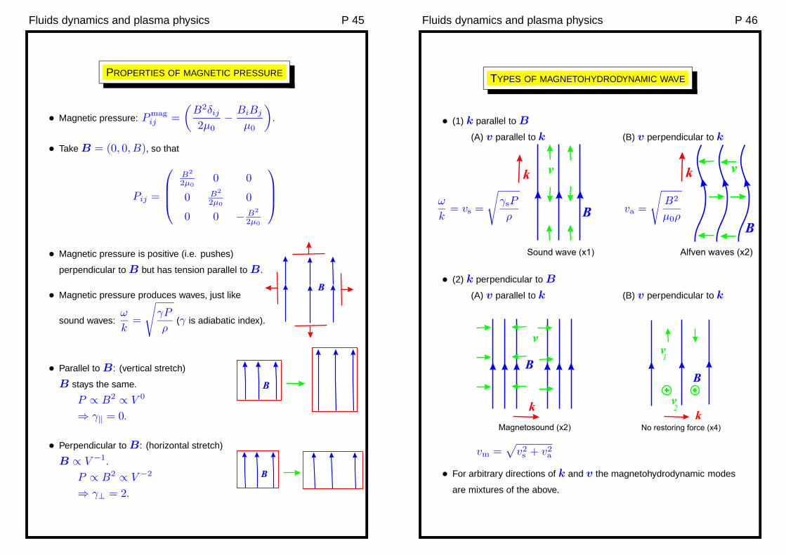
Fluids dynamics and plasma physics P 45
PROPERTIES OF MAGNETIC PRESSURE
• Magnetic pressure: Pmagij =
(
B2δij
2µ0
− BiBj
µ0
)
.
• Take B = (0, 0, B), so that
Pij =
B2
2µ00 0
0 B2
2µ00
0 0 − B2
2µ0
• Magnetic pressure is positive (i.e. pushes)
perpendicular to B but has tension parallel to B.
• Magnetic pressure produces waves, just like
sound waves:ω
k=
√
γP
ρ(γ is adiabatic index).
• Parallel to B: (vertical stretch)
B stays the same.
P ∝ B2 ∝ V 0
⇒ γ‖ = 0.
• Perpendicular to B: (horizontal stretch)
B ∝ V −1.
P ∝ B2 ∝ V −2
⇒ γ⊥ = 2.
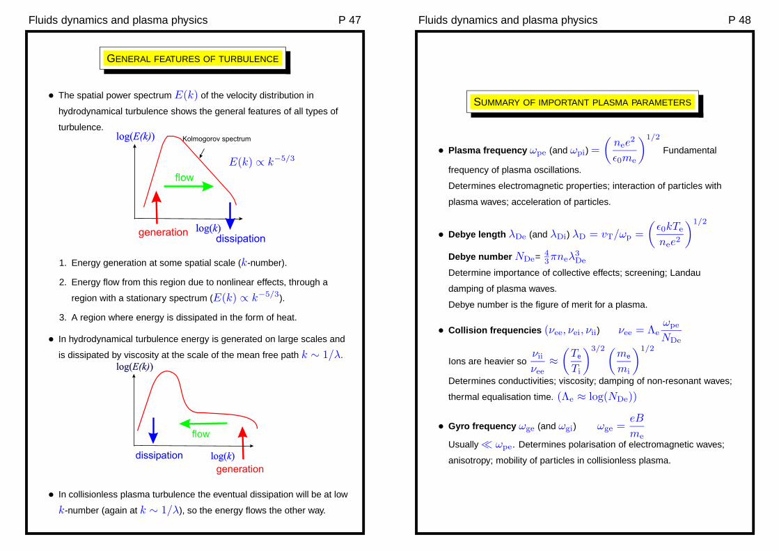
Fluids dynamics and plasma physics P 46
TYPES OF MAGNETOHYDRODYNAMIC WAVE
• (1) k parallel to B
(A) v parallel to k (B) v perpendicular to k
ω
k= vs =
√
γsP
ρva =
√
B2
µ0ρ
• (2) k perpendicular to B
(A) v parallel to k (B) v perpendicular to k
vm =√
v2s + v2
a
• For arbitrary directions of k and v the magnetohydrodynamic modes
are mixtures of the above.
Fluids dynamics and plasma physics P 47
GENERAL FEATURES OF TURBULENCE
• The spatial power spectrum E(k) of the velocity distribution in
hydrodynamical turbulence shows the general features of all types of
turbulence.
E(k) ∝ k−5/3
1. Energy generation at some spatial scale (k-number).
2. Energy flow from this region due to nonlinear effects, through a
region with a stationary spectrum (E(k) ∝ k−5/3).
3. A region where energy is dissipated in the form of heat.
• In hydrodynamical turbulence energy is generated on large scales and
is dissipated by viscosity at the scale of the mean free path k ∼ 1/λ.
• In collisionless plasma turbulence the eventual dissipation will be at low
k-number (again at k ∼ 1/λ), so the energy flows the other way.
Fluids dynamics and plasma physics P 48
SUMMARY OF IMPORTANT PLASMA PARAMETERS
• Plasma frequency ωpe (and ωpi) =
(
nee2
ε0me
)1/2
Fundamental
frequency of plasma oscillations.
Determines electromagnetic properties; interaction of particles with
plasma waves; acceleration of particles.
• Debye length λDe (and λDi) λD = vT/ωp =
(
ε0kTe
nee2
)1/2
Debye number NDe= 43πneλ
3De
Determine importance of collective effects; screening; Landau
damping of plasma waves.
Debye number is the figure of merit for a plasma.
• Collision frequencies (νee, νei, νii) νee = Λe
ωpe
NDe
Ions are heavier soνii
νee
≈(
Te
Ti
)3/2 (
me
mi
)1/2
Determines conductivities; viscosity; damping of non-resonant waves;
thermal equalisation time. (Λe ≈ log(NDe))
• Gyro frequency ωge (and ωgi) ωge =eB
meUsually ωpe. Determines polarisation of electromagnetic waves;
anisotropy; mobility of particles in collisionless plasma.

![L-14 Fluids [3] Fluids at rest Why things float Archimedes’ Principle Fluids in Motion Fluid Dynamics –Hydrodynamics –Aerodynamics.](https://static.fdocuments.in/doc/165x107/56649d9f5503460f94a89e67/l-14-fluids-3-fluids-at-rest-why-things-float-archimedes-principle.jpg)


![L-14 Fluids [3] Fluids at rest Fluids at rest Why things float Archimedes’ Principle Fluids in Motion Fluid Dynamics Fluids in Motion Fluid Dynamics.](https://static.fdocuments.in/doc/165x107/56649d845503460f94a6ab30/l-14-fluids-3-fluids-at-rest-fluids-at-rest-why-things-float-archimedes.jpg)
![L-14 Fluids [3] Fluids in Motion Fluid Dynamics HydrodynamicsAerodynamics.](https://static.fdocuments.in/doc/165x107/56649e705503460f94b6e312/l-14-fluids-3-fluids-in-motion-fluid-dynamics-hydrodynamicsaerodynamics.jpg)

![L-14 Fluids [3] Why things float Fluids in Motion Fluid Dynamics –Hydrodynamics –Aerodynamics.](https://static.fdocuments.in/doc/165x107/56649dea5503460f94ae4fa2/l-14-fluids-3-why-things-float-fluids-in-motion-fluid-dynamics.jpg)


