ISRN LUTMDN/TMHP—12/5262—SE Kkk ISSN 0282-1990

FLUID STRUCTURE INTERACTION A STUDY OF POURING, USING FSI-SIMULATIONS

Nibras Alsuhairi

Thesis for the Degree of Master of Science Division of Fluid Mechanics Department of Energy Sciences Faculty of Engineering Lund University

1

FLUID STRUCTURE INTERACTION A STUDY OF POURING, USING FSI-SIMULATIONS

by

NIBRAS ALSUHAIRI

Supervisor from LTH

Johan Revstedt

Supervisor from Tetra Pak

Michael Olsson

Examination from LTH

Xue-Song Bai

A thesis submitted to the Faculty of Engineering

in partial fulfilment of the requirements for the degree of

Master of Mechanical Engineering

Department of Energy Sciences Division of Fluid Mechanics

Lund University

SEPTEMBER 2012

Faculty of Engineering LTH

2

Acknowledgement

The research presented in this master’s thesis was carried out at Tetra Pak R&D AB in Lund in cooperation with the Division of Energy at the University of Lund, Sweden, during April 2012 to August 2012.

First I would like to express my deepest gratitude to my supervisor M.Sc Michael Olsson at Tetra Pak R&D AB, for his support and guidance throughout this project. Without his assistance this thesis would have been difficult to complete. Further -a great thanks to my supervisor Professor Johan Revstedt at the Division of Energy, for his support with the theory, ideas and useful feedback. A great thank you to Tobias Berg and ANSYS Inc in Gothenburg. This thesis would not been possible to carry out without their help. Finally I would also like to thank the staff at Tetra Pak and especially to Flow Group in Lund for valuable input to the project and for a very fun time during the work.

Lund, September 2012

Nibras Alsuhairi

3

Abstract At Tetra Pak the liquid packages are constantly developed and refined to fill the customer’s needs. A powerful tool is simulation, to evaluate the design of a new package early in the development process.

To determine the performance of beverage packages at Tetra Pak different tests are made in different ways to make secure that they meet the requirements. The pouring performance of a package is a critical parameter, which needs to be considered when developing a new package. In this master’s thesis the pouring case will be considered. The goal is to evaluate the possibilities to perform FSI-, Fluid Structure Interaction, simulations of the dynamic pouring case and develop a simulation strategy for these kinds of simulations. In future Tetra Pak wants to be able to simulate “real” packages to better understand the pouring behaviour. This model can then be used to better understand dynamics, of pouring and make predicting about future packages for various products in a virtual pouring rig.

The FSI-simulations has been performed in the computer software ANSYS Inc. 14.0.0 WorkBench, since this version of ANSYS has the capability of performing strongly coupled FSI- simulation, due to the boundary source coefficient that has been developed. The development of the pouring methodology has been performed on a small conceptual package with a small opening. This work is a continuation of the proof of concept developed by Tobias Berg from ANSYS in Gothenburg. The thesis includes test of the time step, the gulping dynamics, the boundary source coefficient, VOF scheme, Young’s modulus, density, effect of the surface tension and a scale up of volume.

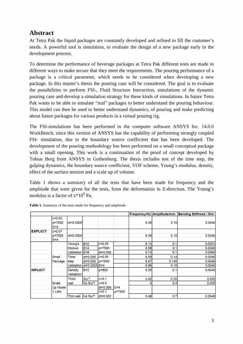
Table 1 shows a summary of all the tests that have been made for frequency and the amplitude that were given for the tests, from the deformation in Z-direction. The Young’s modulus is a factor of x*108 Pa.

Table 1. Summary of the tests made for frequency and amplitude

4

Table of Contents Acknowledgement ..................................................................................................................... 2

Abstract ...................................................................................................................................... 3

Table of Contents ....................................................................................................................... 4

Introduction ................................................................................................................................ 7

Background ............................................................................................................................ 7

Objective .................................................................................................................................. 10

Method ................................................................................................................................. 11

Thesis structure .................................................................................................................... 11

Fluid mechanics ................................................................................................................... 12

CFD ...................................................................................................................................... 13

Turbulence ........................................................................................................................... 14

Large-eddy simulation ......................................................................................................... 15

Structural mechanics ............................................................................................................ 15

Computational Structural Mechanics CSM ......................................................................... 17

Newton-Raphson method................................................................................................. 17

FSI, Fluid Structure Interaction ........................................................................................... 18

Implicit time-marching schemes .......................................................................................... 18

Dirichlet/Neumann subiterations ..................................................................................... 20

Package background ............................................................................................................ 21

Surface tension ..................................................................................................................... 22

Boundary source coefficient ................................................................................................ 23

Fast Fourier Transform -FFT ............................................................................................... 24

Modal Analysis .................................................................................................................... 24

Beam in bending .................................................................................................................. 28

ANSYS ................................................................................................................................ 28

Discretization Methods ........................................................................................................ 29

Finite Element method FEM ................................................................................................ 29

Finite Volume method FVM ................................................................................................ 31

Volume of Fluid VOF .......................................................................................................... 32

Numerical Solution .............................................................................................................. 34

Direct/Explicit Solution Methods ........................................................................................ 35

Iterative Solution Method .................................................................................................... 35

5

Consistency, Stability, Convergence and Accuracy ............................................................ 35

FSI-simulation in ANSYS ....................................................................................................... 37

Modelling ............................................................................................................................. 37

Test 1 Impact of the Boundary Source Coefficients ............................................................ 39

Discussion ........................................................................................................................ 42

Test 2 Explicit versus Implicit- Scheme .............................................................................. 42

Discussion ........................................................................................................................ 43

Test 3 Implicit – time step validation .................................................................................. 43

Discussion ........................................................................................................................ 46

Test 4 Young’s modulus ...................................................................................................... 46

Discussion ........................................................................................................................ 48

Test 5 Density validation ..................................................................................................... 48

Discussion ........................................................................................................................ 49

Test 6 Scale up model to one litre ........................................................................................ 50

Discussion ........................................................................................................................ 51

Test 7 surface tension on one litre package ......................................................................... 51

Thicker wall: .................................................................................................................... 51

Discussion ........................................................................................................................ 54

With and without surface tension .................................................................................... 54

Discussion ........................................................................................................................ 57

Thinner wall: .................................................................................................................... 57

Discussion ........................................................................................................................ 59

Thicker wall- Changed Young’s modulus ....................................................................... 59

Discussion ........................................................................................................................ 61

Test 8 Module Analysis ....................................................................................................... 61

Discussion ........................................................................................................................ 63

Conclusions .......................................................................................................................... 64

Summary .............................................................................................................................. 66

Future work .......................................................................................................................... 66

Reference ................................................................................................................................. 67

6

7

Chapter 1 Introduction

Introduction

Background AB Tetra Pak is a Swedish company, founded in 1951 by Dr. Ruben Rausing in Lund, Sweden. The name Tetra derives from the tetrahedron, which was one of the first milk containers, now known as Tetra Classic. Tetra Pak is one of the leading companies on the liquid carton based packaging industry and Tetra Pak manufacture both filling machines and package materials. To maintain the position as a market leader, constant work is put in development of new packages - and further develop already existing packages. This is done in many stages and one of them is physical testing. These tests requires a lot of time and personnel, at great expense for the company. Because of this, Tetra Pak wants to simulate as many processes as possible virtually, to lower the needs of costly physical testing. In all filling machines in Tetra Pak there is an interaction between package material, filling machine and product. Due to this, simulations in FSI has become much more of interest. These kinds of simulations have from a numerical point of view so far been difficult, since available software has not been ready for the task. As software has matured with newer technology, a strongly coupled simulation of FSI is a possibility. In the future, Tetra Pak wants to be able to simulate “real” packages to better understand the pouring behaviour. This model can then be used to better understand the dynamics of pouring and make predicting about future packages for various products in a virtual pouring rig.

Figure 1 shows some of the packages that Tetra Pak has developed. Figure 2 shows the model Tetra Brik Aseptic 1000.

8

Figure 1. Different Tetra Pak packages [13]

Figure 2. Tetra Brik 1000 ml [13]

Previous attempts to simulate pouring have assumed fixed package material. This is a simplification. However, when compared to experimental data, which was made in Modena, it turned out that the real case had much higher amplitude and lower frequency of the deformation of the package. This was due to that the package could deform inwards, although the package was fixed. This led to the decision of running FSI for the pouring case. Two projects have been carried out in this subject, FSI. One in Abaqus coupled with STAR-CCM+ and one with ANSYS 14.0.0 WorkBench. The explicit coupling in ANSYS was not robust enough with regards on numerical stability, which made the model impossible to run. This master thesis is motivated by taking one large step towards a virtual model system and

9

get a better understanding in the different physical phenomenon that can cause problems in numerical instabilities. The goal is to come up with a simulation strategy for these kinds of simulations.

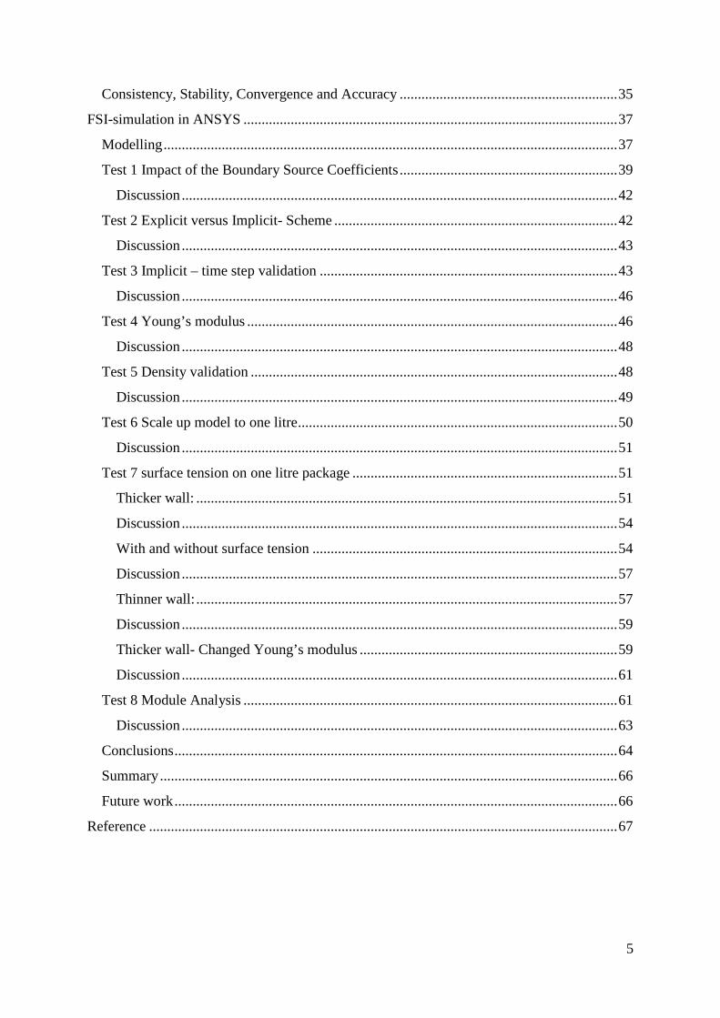
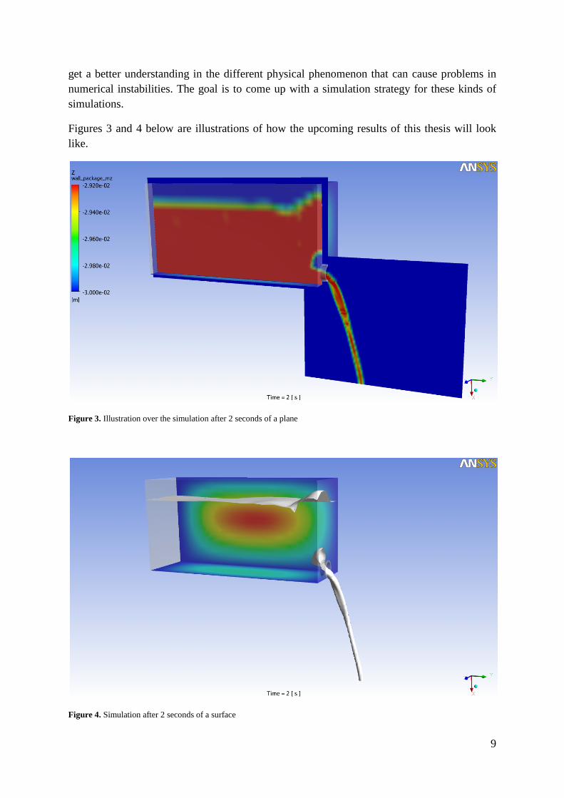
Figures 3 and 4 below are illustrations of how the upcoming results of this thesis will look like.

Figure 3. Illustration over the simulation after 2 seconds of a plane

Figure 4. Simulation after 2 seconds of a surface

10

In this master thesis we have chosen to focus on some parameters, which are more or less critical. The choice of parameters has been done to investigate their impact on numerical stability, since this was unknown. The parameters in this thesis and expected result (before initiating the simulation work) are listed below.

• Boundary source coefficient, investigate the influence on numerical stability of it and if it’s necessary to use at all. Unclear of the impact on the system.

• Young’s modulus, change in the module ought to change the behaviour of the fluid, in case of amplitude and frequency of the deformation. Higher Young’s modulus should give higher frequency and lower amplitude, due to stiffer material.

• Schemes for the VOF fluid interface, implicit/explicit-VOF- reasonable computation time with FSI has to be achieved otherwise Tetra Pak cannot use the model in further development.

• Density of the package material - Unclear of the impact on the system. But due to higher density, which gives higher mass, this ought to lower the amplitude and higher the frequency.

• Surface tension- investigate the impact of it on the system. This is assumed not should not give a big difference in§ pouring performance.

For the pouring case, the gulping phenomenon is of interest for the development and improvement of the package. The gulping is something that appears because of the pressure inside and outside the package and of the fact that more than one phase is involved. The gravitation creates under-pressure, which gives a deformation on the walls. This will make the package walls to deform. When the under-pressure gets too big, air is taken in and a gulp is given. When studying, the package deformation we can get a better understanding of the gulping by looking at the amplitude and the frequency. The amplitude is a measure of how much it bulges in and out of the package. Frequency is a measure of how much the system gulps.

Objective The objective in this master’s thesis is to suggest an improved simulation strategy for FSI for pouring from packages. This is done by gaining knowledge in FSI for the pouring case and by study numerical instabilities of the FSI simulations. This will enable Tetra Pak to better predict pouring performance even before the first prototype. In the future Tetra Pak wants to be able to simulate “real” packages to better understand the models behaviour shown in experiments. This model can then be used to better understand the dynamics of pouring and make predicting about future packages for various products in a virtual pouring rig. If the simulation results and experimental result doesn’t match one needs to reinvestigate the simulation model and ask if the model is correct or possibly lack some important physics in the model.

To be able to carry out this thesis and achieve the objective, a made model by Tobias Berg from ANSYS has been used, which is a basic model of a TBA-like package and is scaled to 0.13 litres and of the material steel but with a Young’s modulus of 400 MPa. Steel as the

11

material was selected because of that it’s an isotropic material, which is suitable for a basic model.

Method To achieve the objective, the software ANSYS Inc 14.0.0 is used for the simulation. The methodology of the work is divided into eight different test cases. Test 1 evaluates the boundary source coefficient. Test 2 is done to compare explicit vs. implicit VOF-schemes. Furthermore, Test 3 was made to validate the time step. Test 4 is done to evaluate Young’s modulus. A density comparison was made in test 5. In Test 6 a scale up was made to get a package of one litre. In Test 7, the surface tension is in count and set to 0.072 between water and air and in Test 8 a module analysis was made.

Thesis structure In chapter two a discussion of the theory is provided where the reader can get more knowledge on Fluid mechanics, CFD, turbulence, structure mechanics, computational structural mechanics, FSI, package properties, surface tension, boundary source coefficient, FFT and Modal analysis. Chapter 3 describes the discretization methods and numerical analysis of what has been used for this thesis. Chapter 4 contains the FSI implementation and results from this with discussion parts. Finally, chapter 5 involves concluding remarks such as a summary and future work.

12

Chapter 2 Theory

Fluid mechanics Fluid mechanics is the study of fluids (liquids and gases) and the forces acting on them. Fluid mechanics are often divided into fluid statics (fluids at rest), fluid kinematics (fluids in motion) and fluid dynamics (effects or forces on fluid motion). Fluid mechanics is a division of continuum mechanics, which means that the model which is studied is treated as a continuous mass, rather than as discrete particles. Fluid mechanics can be very complex especially when going into mathematical analysis. In those cases the best way to solve the system is by numerical methods with the use of computers. Computation fluid dynamics, CFD, is a discipline which solves fluid mechanics problem numerically. [1]

To study fluids mechanics, the most common approach is to use the continuum mechanics. The governing equations of fluid dynamics represent the fundaments in CFD. They are mathematical statements of the conservation laws of physics which involve mass, momentum and energy. The equations that will be expressed below are not fully derived and it’s up to the reader’s interest to look that up (which are found in most fluids dynamics and CFD books) [2]

The scalar transport equation below expresses a general transport equation:

𝜕𝜌𝜙𝜕𝑡

+ ∇𝜌𝑢𝑖𝜙 = ∇(Γ∇𝜌𝜙) + 𝑆 (2.1)

where 𝜙 is the specific quantity, 𝑢𝑖 the velocity vector, Γ the diffusion coefficient, 𝜌 the density and 𝑆 the source term. The commonalities between equations are shown from this equation. The different terms are referred to as storage, convection, diffusion and generation. The conservative equation of mass and momentum of a fluid flow can on differential form be expresses as:

𝜕𝜌𝜕𝑡

+ 𝜕𝜌𝑢𝑖𝜕𝑥𝑖

= 0 (2.2)

𝜕𝜌𝑢𝑖𝜕𝑡

+ 𝜕𝜌𝑢𝑖𝑢𝑗𝜕𝑥𝑗

= 𝜕𝜏𝑖𝑗𝜕𝑥𝑗

+ 𝜌𝜙𝑖 (2.3)

The mass conservation can for incompressible flows (no change in density over time):

𝜕𝑢𝑖𝜕𝑥𝑖

= 0 (2.4)

where 𝑢𝑖 is the velocity, 𝜌 the density, 𝜙𝑖 the body force per unit volume and 𝜏𝑖𝑗 is the stress tensor.

By assuming a Newtonian fluid, stress versus strain rate curve is linear and passes through the origin with constant proportionality known as viscosity, the stress tensor is then given by:

13

𝜏𝑖𝑗 = −𝑝𝛿𝑖𝑗 + 𝜇 �𝜕𝑢𝑖𝜕𝑥𝑗

+ 𝜕𝑢𝑗𝜕𝑥𝑖� + 𝜆 𝜕𝑢𝑘

𝜕𝑥𝑘𝛿𝑖𝑗 (2.5)

where 𝑝 is the pressure, 𝜇 the dynamic viscosity and 𝛿𝑖𝑗 the Kronecker delta function.

Now assuming incompressibility to a Newtonian fluid then the momentum equation leads to the Navier-Stokes equations shown below:

𝜕𝑢𝑖𝜕𝑡

+ 𝑢𝑗𝜕𝑢𝑖𝜕𝑥𝑗

= − 1𝑝𝜕𝜌𝜕𝑥𝑖

+ 𝑣 𝜕𝜕𝑥𝑗

𝜕𝑢𝑖𝜕𝑥𝑗

+ 𝜙𝑖 (2.6)

where 𝑣 is the kinematic viscosity.

The energy equation is derived in the same manner where the net time rate change of energy equals the net rate of heat added and net work done resulting in following equation.

𝜕𝜌𝐸𝜕𝑡

+ 𝜕𝜌𝑢𝑖𝐸𝜕𝑥𝑗

= 𝜌𝜕𝑞𝜕𝑡

+ 𝜕𝜕𝑥𝑖

�𝑘𝜕𝑇𝑖𝜕𝑥𝑖

�+ 𝜕𝑢𝑖𝜏𝑖𝑗𝜕𝑥𝑖

− 𝜕𝑝𝑢𝑖𝜕𝑥𝑖

+ 𝜌𝑢𝑖 (2.7)

In fluid dynamics the Reynolds number, Re, is a dimensionless number that provides a measure of the ratio of inertial forces to viscous forces and thus quantifying the relative importance of these two types of forces for given flow.

Reynolds number 𝑅𝑒 = 𝑈𝐿𝑣

= 𝑖𝑛𝑒𝑟𝑡𝑖𝑎𝑙 𝑓𝑜𝑟𝑐𝑒𝑠𝑣𝑖𝑠𝑐𝑜𝑢𝑠 𝑓𝑜𝑟𝑐𝑒𝑠

where 𝑣 is the kinematic viscosity. ´

CFD Computational fluid dynamics, CFD, which is derived from various disciplines in fluid mechanics and heat transfer, has become an important area, especially in process industry, chemical, and medical technology. The application of computational simulations for new product development and evaluation of existing equipment, resulting in system optimization and increased efficiency which in turn leads to lower costs and decrease for the redevelopment, has made CFD an important tool for industry and therefore a branch of fluid mechanics and computer world. The fluid mechanics is essentially the study of fluids either in motion or at rest. CFD is specifically designed for fluids in motion and how the fluid flow behaviour affects processes, there of the "fluid dynamics" in the terminology. The physical properties of fluid motion are usually described by basic mathematical equations, often in partial differential equations, and are commonly called "governing equations" in CFD. To solve these mathematical equations they are converted to computer programs or software packages. The C in CFD is the study of the fluid flow through numerical simulations, which involve the use of computer programs used in digital computers to obtain numerical solutions.

Tetra Pak has an interest in CFD because of the fact that in the future, they want to be able to simulate “real” packages to better understand the models behaviour according to experiments. This model can then be used to better understand the dynamics of pouring and make predictions about future packages for various products in a virtual pouring rig. If the

14

simulation results and experimental result doesn’t match one needs to reinvestigate the simulation model and ask if the model is correct or possibly lack some important physics in the model.

The derived equations that were represented in the part of Fluid Mechanics for momentum all includes pressure and velocity field, although there is no explicit equation for pressure, looking at continuity and momentum one finds four equations and four variables. For incompressible flows, the pressure-velocity coupling algorithms are used to derive equations for the pressure from momentum and continuity equation. One of the most common algorithms is the so called SIMPLE algorithm, although there are other more improved once such as SIMPLEC and PISO. Depending on the flows behaviour one algorithm is faster for that case.

A CDF analysis can be summarized with some steps which include; problem identification, pre-processing and solver execution and post-procession. [2]

Turbulence For high velocities, and there by high Reynolds number, the flow undergoes transition to turbulence. This makes the flow more complex and unstable. In the study of turbulent flow the ultimate goal is to have a convenient and quantitative model that can be used to calculate the amounts of interest and practical relevance. To reflect on the characteristics of the turbulent flow from the very beginning pays off when choosing right turbulence model, this is due to the difficulties that arise with the turbulence. There is always a difficulty to simulate turbulence at high Reynolds number, this is because it requires large computer capacity but also the assumptions one make when creating the turbulence model, which allows the errors in the result becoming large in some circumstances.

Needless to say, accuracy is something to strive for of each model. In the simulation, the accuracy of the model is determined by comparing the modelled results with the experimental measurements. The numerical solution of the model contains inevitably numerical errors than can be from several sources, but it is usually from spatial truncation errors. There is no "best" model, but rather a series of models that can be applied to different cases of turbulent flow.

For the simulation where turbulence arises, a choice of turbulence model is made. By averaging the governing equations will lead to an unclosed system. Therefor turbulence models have to be used to be able to solve the system and close it. The most widely used types of turbulence model are the so-called two-equation models, such as k-ε model and k- ω model. These models are based on averaging of the governing equations and Boussinesqs hypothesis. [3]

The governing equations for the problem are described below:

Conservation of mass:

𝜕𝑢𝑖�𝜕𝑥𝑖

= 0

15

Conservation of momentum:

𝜕𝑢𝑖�𝜕𝑡 + 𝑢𝑗�

𝜕𝑢𝑖�𝜕𝑥𝑗

= −1𝜌�

𝜕𝑝𝜕𝑥𝑖

�+ 𝑣�𝜕2𝑢𝑖𝜕𝑥𝑗2

�−𝜕𝑢𝑖́ 𝑢𝑗́�������

𝜕𝑥𝑗

In this master thesis a Large Eddy Simulation, LES, was chosen for the turbulence model.

Large-eddy simulation In Large-eddy simulation, LES, one focus on the large eddies that appear in the model, whereas the effects of the smaller scales are modelled. Due to the fact that in LES the unsteady motions of the large-scales are represented explicitly once expected that the LES is more accurate and reliable then Reynolds-stress models for flows in which large-scale turbulence is significant.

The dynamics of the larger-scale motions, which are not universal and affected by the flow geometry, are computed explicit in LES. Simple model represents the smaller scales, which have up to some level a universal character.

There are four conceptual steps according to Stephen B. Pope [3] in LES, which are presented below:

“

- A filtering operation is defined to decompose the velocity U(x,t) into the sum of a filtered (or resolved) component 𝑈�(𝒙, 𝑡) and a residual (or subgrid-scale, SGS) component u’(x, t). The filtered velocity field 𝑈�(𝒙, 𝑡) -which is three-dimensional and time-dependent- represents the motion of the large eddies.

- The equations for the evolution of the filtered velocity field are derived from the Navier-Stokes equations. These equations are of the standard form, with the momentum equation containing the residual-stress tensor (or SGS stress tensor) that arises from the residual motions.

- Closure is obtained by modelling the residual-stress tensor, most simply by an eddy-viscosity model.

- The model filtered equations are solved numerically for 𝑈�(𝒙, 𝑡), which provides an approximation to the large-scale motions in one realization of the turbulent flow. “[3]

Structural mechanics Structural mechanics refers to the physics of solids that are composed of slender elements such as beams, plates and shells. To study the behaviour of structural mechanics, continuum mechanics are used. One of the most fundamental relations within solid mechanics is the principle of virtual work. From this expression most of the engineering relations can be derived. It states that external forces or work is equal to internal, due to internal stresses. [4]

16

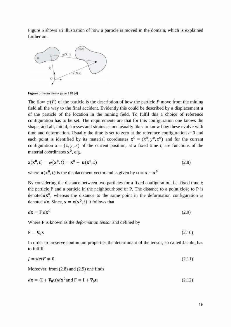
Figure 5 shows an illustration of how a particle is moved in the domain, which is explained further on.

Figure 5. From Krenk page 118 [4]

The flow 𝜑(𝑃) of the particle is the description of how the particle P move from the mining field all the way to the final accident. Evidently this could be described by a displacement u of the particle of the location in the mining field. To fulfil this a choice of reference configuration has to be set. The requirements are that for this configuration one knows the shape, and all, initial, stresses and strains as one usually likes to know how these evolve with time and deformation. Usually the time is set to zero at the reference configuration t=0 and each point is identified by its material coordinates 𝐱𝟎 = (𝑥0,𝑦0, 𝑧0) and for the currant configuration 𝐱 = (𝑥,𝑦 , 𝑧) of the current position, at a fixed time t, are functions of the material coordinates 𝐱𝟎, e.g.

𝐱(𝐱𝟎, 𝑡) = 𝜑(𝐱𝟎, 𝑡) = 𝐱𝟎 + 𝐮(𝐱𝟎, 𝑡) (2.8)

where 𝐮(𝐱𝟎, 𝑡) is the displacement vector and is given by 𝐮 = 𝐱 − 𝐱𝟎

By considering the distance between two particles for a fixed configuration, i.e. fixed time t; the particle P and a particle in the neighbourhood of P. The distance to a point close to P is denoted𝑑𝐱𝟎, whereas the distance to the same point in the deformation configuration is denoted 𝑑𝐱. Since, 𝐱 = 𝐱(𝐱𝟎, 𝑡) it follows that

𝑑𝐱 = 𝐅 𝑑𝐱𝟎 (2.9)

Where F is known as the deformation tensor and defined by

𝐅 = 𝛁𝟎𝐱 (2.10)

In order to preserve continuum properties the determinant of the tensor, so called Jacobi, has to fulfill:

𝐽 = 𝑑𝑒𝑡𝑭 ≠ 0 (2.11)

Moreover, from (2.8) and (2.9) one finds

𝑑𝐱 = (𝐈 + 𝛁𝟎𝐮)𝑑𝐱𝟎and 𝐅 = 𝐈 + 𝛁𝟎𝐮 (2.12)

17

For most analysis the stress tensor S is used and is defined by

𝐒 = 12

(𝐂 − 𝐈) (2.13)

where the Cauchy-Green’s deformation tensor is defined as

𝐂 = 𝐅𝐓𝐅 (2.14)

Giving the expression for the stress tensor as:

𝐒 = 12

(𝛁𝟎𝐮 + (𝛁𝟎𝐮)𝐓 + (𝛁𝟎𝐮)𝐓𝛁𝟎𝐮) (2.15)

One parameter that is of interest in this master thesis is Young’s modulus which is defined as:

𝐸 = 𝜎𝜖

=𝑁𝐴

𝑙−𝑙0𝑙0

(2.16)

where N is the force on the surface area A, l is the length after deformation and l0 is the length from time zero.

Computational Structural Mechanics CSM The FEM-method is by far the most used discretization method for solving CSM methods. The steps can be summarized as; introduce the FEM approximation of the quantity of interest, e.g. displacement and weight function. Use a shape function as integrate over the entire domain.

The governing system of equation used in FEM, as described in the FEM chapter later on, is:

𝑀�̈�(𝑡) + 𝐷�̇�(𝑡) + 𝐹𝑖𝑛𝑡𝑢(𝑡) = 𝐹𝑒𝑥𝑡𝑢(𝑡) (2.17)

where M is the mass matrix, D the damping matrix, 𝐹𝑖𝑛𝑡 the internal force and 𝐹𝑒𝑥𝑡 the external load on the structure.

For most systems the linear relationship is not valid, e.g. Hooke’s law; F=-ku, where k is the stiffness and u the displacement. Solution methods for non-linear transient problem are case dependent due to the fact that there exists a variation of linearization and time integration methods. One of the most used methods for solving non-linear system is the Newton-Rahpson method, and is used in Ansys Mechanical for this master thesis. [4]

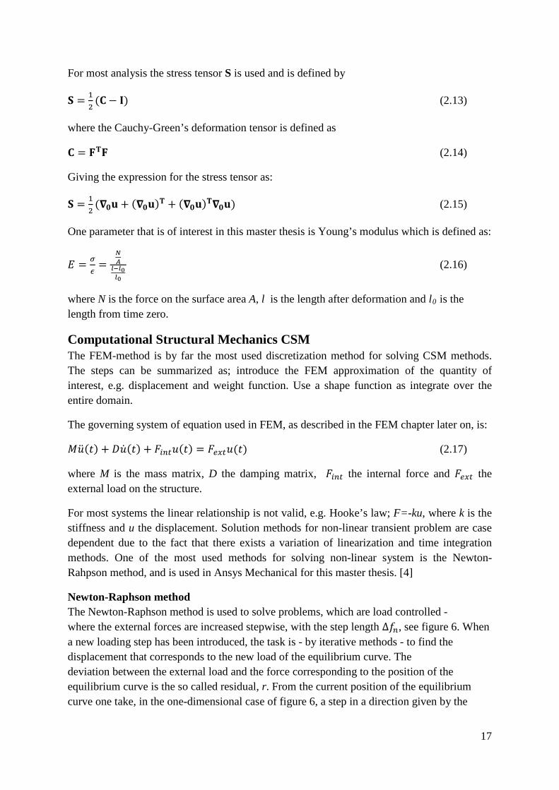
Newton-Raphson method The Newton-Raphson method is used to solve problems, which are load controlled - where the external forces are increased stepwise, with the step length ∆𝑓𝑛, see figure 6. When a new loading step has been introduced, the task is - by iterative methods - to find the displacement that corresponds to the new load of the equilibrium curve. The deviation between the external load and the force corresponding to the position of the equilibrium curve is the so called residual, r. From the current position of the equilibrium curve one take, in the one-dimensional case of figure 6, a step in a direction given by the

18

curve tangent at that point and have the same height as the residual of the point. Since the curve is not linear, we obtains a new residual and, therefore, a new iteration step is made. These iterations are continued until the residual reaches a selected tolerance, usually in the size of 10−6. When the residual is sufficiently small, a new load step is taken and subsequently performed iterations to reach equilibrium. The load step is taken until the total external load is applied. [4]

Figure 6. Illustration of Newton-Raphson method. (Picture from Krenk, page 11) [4]

FSI, Fluid Structure Interaction Fluid Structure Interaction, FSI, is the study between fluids and structures and is an aspect common in most natural phenomena and is a branch of multi-physics. It is the interaction of some movable or deformable structure with an internal or surrounding fluid flow. Fluid–structure interactions can be stable or oscillatory. In oscillatory interactions, the strain induced in the solid structure causes it to move such that the source of strain is reduced, and the structure returns to its former state only for the process to repeat.

O.C. Zienkiewicz and R. Taylor [5] state the full definition of FSI as:

“Coupled system and formulations are those applicable to multiple domain and depend variables which usually describe different physical phenomena and in which neither domain can be eliminated at the different equation level”

There are two different approaches of FSI, one is the monolithic or simultaneous approach, which refers to that the equations governing the flow and the displacements of the structure are solved simultaneously, with a single solver. The other one is the partitioned or segregated approach, which can be divided into implicit coupling or explicit coupling. In this approach the equations governing the flow and the displacement of the structure are solved separately, with two distinct solvers.

Implicit time-marching schemes For some FSI systems, the explicit algorithm might not work. This makes it obvious to switch to implicit coupling algorithms. By combining the Euler scheme for the fluid with the first

19

order backward difference scheme for the structure, IE-BDF scheme, we obtain the time-discrete problem as: [6]

𝜌𝑓𝑢𝑛+1−𝑢𝑛

𝛿𝑡+ ∇𝑝𝑛+1 = 0

𝑑𝑖𝑣 𝑢𝑛+1 = 0

𝑝𝑛+1 = �̅�(𝑡𝑛+1)

𝑢𝑛+1 ∗ 𝑛 = 0

𝑢𝑛+1 ∗ 𝑛 = 𝜂𝑛+1−𝜂𝑛

𝛿𝑡 (2.19)

𝜌𝑠ℎ𝑠𝜂𝑛+1−2𝜂𝑛+𝜂𝑛−1

𝛿𝑡2+ 𝑎𝜂𝑛+1 = 𝑝𝑛+1 (2.20)

This problem corresponds to the following discrete added-mass problem for the structure

(𝜌𝑠ℎ𝑠 + 𝜌𝑓𝑀𝐴) 𝜂𝑛+1−2𝜂𝑛+𝜂𝑛−1

𝛿𝑡2+ 𝑎𝜂𝑛+1 = 𝑝𝑒𝑥𝑡𝑛+1 (2.21)

where 𝜂 is the wall displacement, 𝛿𝑡 the time step, 𝑡 time, 𝑢 fluid displacement, 𝑢 fluid pressure, 𝜌𝑓 density for the fluid, 𝜌𝑠 density for the structure and the operator 𝑀𝐴:𝐻−1/2 →𝐻1/2 is defined as:

𝑀𝐴𝑤 = 𝑅𝑤 (2.22)

and is a continuous operator, where 𝑤 are given functions , and 𝑤 ∈ 𝐻−1/2 denotes 𝑅𝑤.

For complex, and often realistic, situations the problem might be non linear in the fluid and/or in the structure equations and cause possibly large displacements of the structure. In order to solve these kinds of systems in each time step it is convenient to use an iterative methods, which allow to decuple the fluid from the structure step and, ultimately, to use already available computer codes.

One common used scheme to solve these kind of complex systems is the Dirichlet/Neumann subiterations, D-N. By D-N one referrers to that on each iteration one solve the fluid equations with respect to primitive variables (u, p) subject to Dirichlet boundary conditions, see equation 2.23 below, at the interface (imposed displacements or velocities) and the structure equations subjected to Neuman boundary conditions (imposed loads), see equation 2.24 below. [6]

Dirichlet boundary condition prescribes the value of a variable at the boundary [2]

𝜙(𝑥) = 𝑐𝑜𝑛𝑠𝑡𝑎𝑛𝑡 (2.23)

(2.18)

20

Neumann boundary condition prescribes the gradient normal to the boundary of a variable [2]

𝜕𝜙(𝑥)𝜕𝑛

= 𝑐𝑜𝑛𝑠𝑡𝑎𝑛𝑡 (2.24)

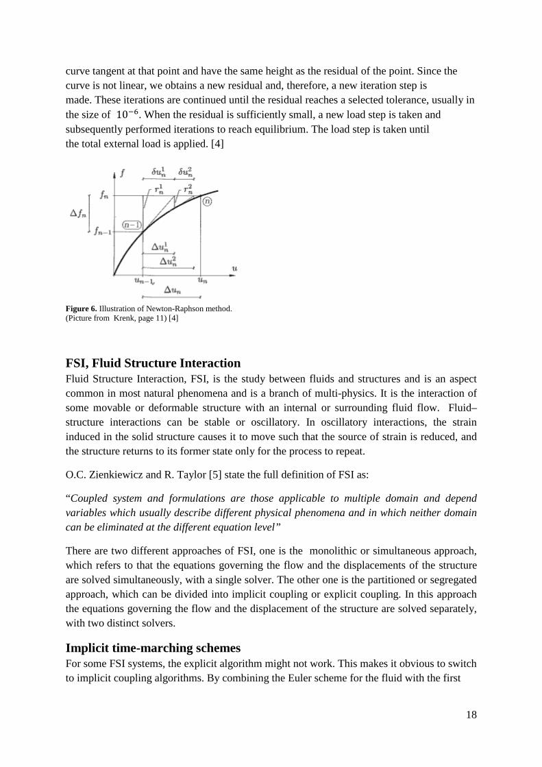
Dirichlet/Neumann subiterations At each time step, using the following algothm to solve (2.18) to (2.21) : Given an initial guess 𝜼𝟎𝒏+𝟏 and solv for 𝒌 = 𝟏,𝟐, …

Fluid step: find (𝒖𝒌,𝒑𝒌) s.t.

𝜌𝑓𝑢𝑘−𝑢𝑛

𝛿𝑡+ ∇𝑝𝑘 = 0

𝑑𝑖𝑣 𝑢𝑘 = 0

𝑝𝑘 = �̅�(𝑡𝑛+1)

𝑢𝑘 ∗ 𝑛 = 0

𝑢𝑘 ∗ 𝑛 = 𝜂𝑘−1−𝜂𝑛

𝛿𝑡

1. Structure step: find 𝜂𝑘� s.t.

𝜌𝑠ℎ𝑠𝜂𝑘� −2𝜂𝑛+𝜂𝑛−1

𝛿𝑡2+ 𝑎𝜂𝑘� = 𝑝𝑘

2. Relaxation step:

𝜂𝑘 = 𝜔𝜂𝑘� + (1 − 𝜔)𝜂𝑘−1

3. Convergence test: • if ‖𝜂𝑘 − 𝜂𝑘−1‖ < 𝑡𝑜𝑙 then set 𝜂𝑛+1 = 𝜂𝑘, 𝑢𝑛+1 = 𝑢𝑘 and 𝑝𝑛+1 = 𝑝𝑘 • else set 𝑘 = 𝑘 + 1 and go to step 1.

where 𝜂𝑘� = 𝜂𝑘𝜔− 1−𝜔

𝜔𝜂𝑘−1

21

Package background Tetra Pak packaging material is made of different layers, including carton, polymer and aluminium. This makes the modelling and simulation from a structural mechanical point of view hard, due to the fact that both plastic and paper are nonlinear material and paper is anisotropic material.

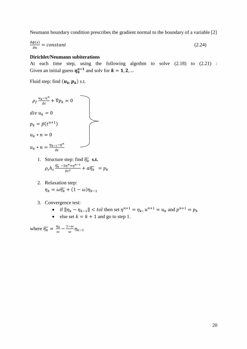
By assuming that the package is not stretched above the yielding limit, it is working in the range of elastic plastic, a simple equilibrium balance can be done to get the correct Young’s modulus for the system in different directions, which is seen below.

Equilibrium for the force balance gives:

𝜎𝐴 = 𝜎1𝐴1 + 𝜎2𝐴2 𝐸𝜀𝐴 = 𝐸1𝜀1𝐴1 + 𝐸2𝜀2𝐴2

𝐸ℎ = 𝐸1ℎ1 + 𝐸2ℎ2

𝐸 = 𝐸1ℎ1+𝐸2ℎ2 ℎ

or as 𝐸 = ∑𝐸𝑖ℎ𝑖∑ℎ𝑖

depending on who many layers the system involves in.

where hi is the thickness of each layer, 𝜎 is the shear stress, 𝐴𝑖 is the area for each layer, 𝐸𝑖 is Young’s modulus for each layer and 𝜀 is the strain.

The papers behaviour is anisotropic, the property of being directionally dependent. In the anisotropic continuum model the elastic behaviour is assumed to be different in the machine direction, MD, cross direction, CD and in z-axial direction, ZD. Therefore, the linear elastic behaviour is represented by 9 different elastic constants: 𝐸1,𝐸2,𝐸3,𝐺12,𝐺13,𝐺23 and 𝑣12, 𝑣13, 𝑣23. Where E is Young’s modulus, G is the shear module and v is poisons ratio. The used yield criteria accounts for different yields stresses in different directions through Hill’s criteria. Hill’s yield criterion is defined as: [7]

𝑓 = �𝐹(𝝈22 − 𝝈33)2 + 𝐺(𝝈33 − 𝝈11)2 + 𝐻(𝝈11 − 𝝈22)2 + 2𝐿𝝈232 + 2𝑀𝝈312 + 2𝑁𝝈122 (2.25)

where

𝐹 = 𝝈𝑀𝐷2

2� 1

(𝝈22𝑠 )2 + 1

�𝝈33𝑠 �2

− 1(𝝈11

𝑠 )2� = 12� 1𝑅222

+ 1𝑅332

− 1𝑅112� (2.26)

𝜎1𝐴1

𝜎2𝐴2

𝜎𝐴

22

𝐺 = 𝝈𝑀𝐷2

2� 1

�𝝈33𝑠 �2

+ 1(𝝈11

𝑠 )2 −1

(𝝈22𝑠 )2� = 1

2� 1𝑅332

+ 1𝑅112

− 1𝑅222� (2.28)

𝐻 = 𝝈𝑀𝐷2

2� 1

(𝝈11𝑠 )2 + 1

(𝝈22𝑠 )2 −

1

�𝝈33𝑠 �2

� = 12� 1𝑅112

+ 1𝑅222

− 1𝑅332� (2.29)

𝐿 = 32�𝝈𝑀𝐷𝝈23𝑠 �

2= 3

2𝑅232 (2.30)

𝑀 = 32�𝝈𝑀𝐷𝝈13𝑠 �

2= 3

2𝑅132 (2.31)

𝑁 = 32�𝝈𝑀𝐷𝝈12𝑠 �

2= 3

2𝑅122 (2.32)

Surface tension

When discussing surface tension and surface energy we consider only liquids that resist an external force, and do not support residual stresses, e.g, Newtonian fluids. The dimension of surface tension is force per unit length, and for surface energy it is energy per unit area. The last one is mostly applied for solids and not just liquids. For solids the surface to be stretched mostly needs high stresses from the surface tension, which can result in residual stresses as well as in elastic and plastic deformations. [8]

To take into account the energy required to form the interface between the phases, we need to extend the definition of work. The thermodynamics of interfaces was discussed by Gibbs (1931) in terms of conceptual dividing surface between the phases. This leads to that the principle of work can be written as:

−𝑑𝑊 = −𝑃𝑑𝑉 + ∑ 𝜇𝑖𝑑𝑛𝑖 + 𝜎𝑑𝐴𝑘𝑖=1 (2.33)

where 𝜎 is the surface tension (or surface energy per unit area) and A is the surface area of the interface.

Thus,

𝑑𝑈 = 𝑇𝑑𝑆 − 𝑃𝑑𝑉 + 𝜎𝑑𝐴 + ∑ 𝜇𝑖𝑑𝑛𝑖𝑘𝑖=1 (2.34)

and

𝑑𝐺 = −𝑆𝑑𝑇 + 𝑉𝑑𝑃 + 𝜎𝑑𝐴 + ∑ 𝜇𝑖𝑑𝑛𝑖𝑘𝑖=1 (2.35)

Therefore, the surface energy is the change in the Gibbs free energy per unit area, i.e.,

𝜎 = 𝜕𝐺𝜕𝐴

|𝑇,𝑃,𝑛𝑖 (2.36)

23

By stating that for equilibrium under conditions of constant temperature, and pressure one gets:

𝑑𝐺|𝑇,𝑃 = 𝜎𝑑𝐴+∑ 𝜇𝑖𝑑𝑛𝑖𝑘𝑖=1 ≤ 0 (2.37)

And if chemical equilibrium is guaranteed, 𝜇𝑖1 = 𝜇𝑖2.

∴ 𝜎𝑑𝐴 ≤ 0 ⇒ 𝑑𝐴 ≤ 0 (2.38)

Thus a system in equilibrium tends to minimize the interface area.

𝐹𝑜𝑟𝑐𝑒 𝑏𝑎𝑙𝑎𝑛𝑐𝑒 𝑖𝑛 𝑥 𝑑𝑖𝑟𝑒𝑐𝑡𝑖𝑜𝑛:

(𝜌𝑔ℎ + 𝑃𝑢) 𝜋𝐷2

4− 𝑃𝑎

𝜋𝐷2

4− 𝛾𝜋𝐷 = 0 (2.39)

where 𝛾 is the surface tension, 𝑃𝑢 is the pressure inside the package, 𝑃𝑎 is the atmosphere pressure, h is the high and D is the diameter.

In this work a value of 𝛾 = 0.072 N/m is used, which corresponds to a air- water surface tension at 20oC.

Boundary source coefficient The boundary source coefficient, C, is a constant value which is added in the diagonal of the pressure equation, or more generally, continuity, to get dominance of the system. The on-diagonal block of matrix is demonstrated below

�𝑎𝑝𝑝 + 𝐶 𝑎𝑝𝑣𝑎𝑣𝑝 𝑎𝑣𝑣

� �∆𝑝∆𝑉� = �𝑅𝑝𝑅𝑣� (2.40)

where p is the coefficient for continuity and v for momentum. 𝑎𝑝𝑣 is one of the velocity coefficient in the pressure equation, ∆𝑝 is the pressure update for the current non-linear iteration and 𝑅𝑝 is the continuity residual for the current non-linear iteration. The objective is that at convergence, ∆𝑝 goes to zero, the effective contribution due to the C coefficient tends to zero. This will give the result of that convergence will be stabilized, but the converged solution is not changed. [9]

By adding the coefficient to the diagonal will make the system less stiff.

𝜌𝑔ℎ D

𝑃𝑢 𝑃𝑎

24

Fast Fourier Transform -FFT The Fast Fourier Transform, FFT, is a useful mathematical tool for digital signal processing. With a FFT algorithm one can compute the Discrete Fourier Transform (DFT) and its inverse. In DFT one decomposes a sequence of values into components of different frequencies, which is useful in many fields but can be very slow when computing it directly from the definition. By doing an FFT, which simply is a highly optimized implementation of the DFT, gives the same results but quicker. This has made the FFT very important in many applications, from digital signal processing and solving partial differential equations to algorithms for quick multiplication of large integers. Besides the economic advantages of FFT, there are certain applications where high-speed processing is essential. Real-time radar-echo processing is one such example. [17] [18]

The Fourier transform is defines as:

𝐺(𝑓) = ∫ 𝑔(𝑥)𝑒−𝑗2𝜋𝑓𝑥𝑑𝑥 ∞−∞ (2.41)

𝑔(𝑥) = ∫ 𝐺(𝑓)𝑒𝑗2𝜋𝑓𝑥𝑑𝑓∞−∞ (2.42)

The Discrete Fourier Transform is defined as:

𝐺𝑙 = ∑ 𝑔𝑘𝑒−𝑗2𝜋𝑘𝑙/𝑁𝑁−1𝑘=0 (2.43)

𝑔𝐾 = 1𝑁∑ 𝐺𝑙𝑒−𝑗2𝜋𝑘𝑙/𝑁𝑛−1𝑙=0 (2.44)

Due to the fact that equation (2.43) and (2.44) are basically equivalent, equation (2.43) can be rewritten in a simpler form as:

𝐺𝑙 = ∑ 𝑔𝑘𝑊𝑘𝑙𝑁−1𝑘=0 𝑤ℎ𝑒𝑟𝑒 𝑙 = 0, 2, 3, … ,𝑁 − 1 (2.45)

𝑊 = 𝑒−𝑗2𝜋𝑁 (2.46)

In most programs, such as MatLab or Python, there are functions such as fft( ), which solves the problem. In this thesis, Python has been used.

Modal Analysis Modal analysis is a branch in mechanics and is the study of the dynamic properties of structures under excitation. By analysing the dynamic response of the structure and the fluid when it has been excited by an input, one can get measurements for the modal analysis. [19]

The analysis of the signals typically relies on Fourier analysis. The resulting transfer function will show one or more resonances, whose characteristic mass, frequency and damping can be estimated from the measurements. Modal analysis is very useful in NVH - noise - vibration,

25

and harshness - systems. The results can also be used to correlate with Finite element analysis normal mode solutions.

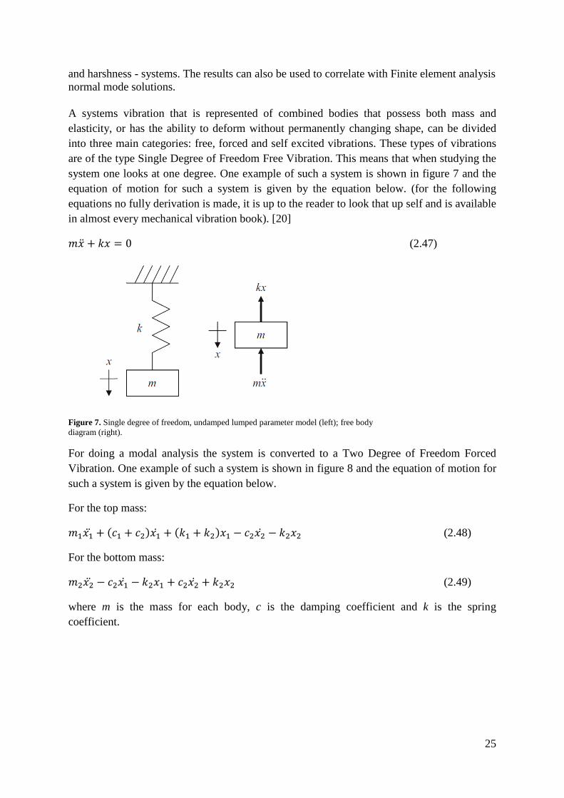
A systems vibration that is represented of combined bodies that possess both mass and elasticity, or has the ability to deform without permanently changing shape, can be divided into three main categories: free, forced and self excited vibrations. These types of vibrations are of the type Single Degree of Freedom Free Vibration. This means that when studying the system one looks at one degree. One example of such a system is shown in figure 7 and the equation of motion for such a system is given by the equation below. (for the following equations no fully derivation is made, it is up to the reader to look that up self and is available in almost every mechanical vibration book). [20]

𝑚�̈� + 𝑘𝑥 = 0 (2.47)

Figure 7. Single degree of freedom, undamped lumped parameter model (left); free body diagram (right).

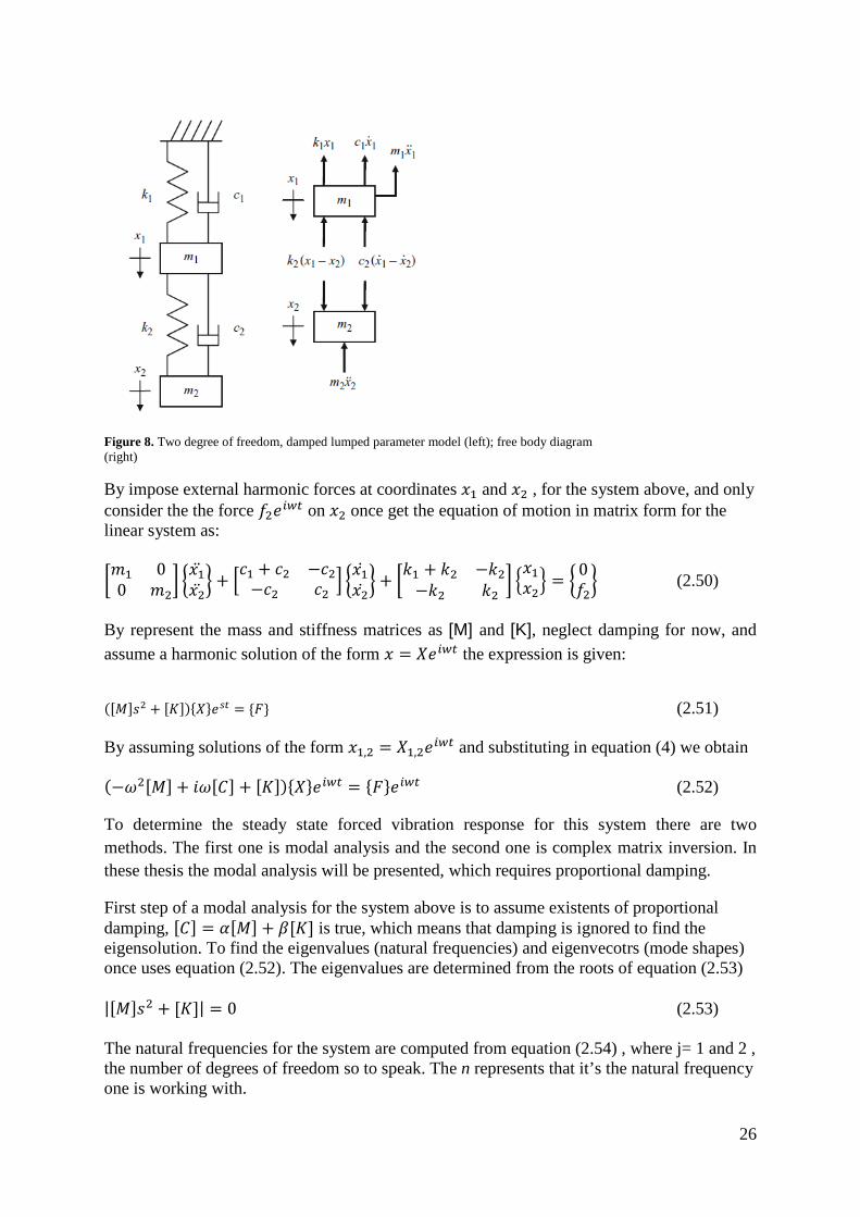
For doing a modal analysis the system is converted to a Two Degree of Freedom Forced Vibration. One example of such a system is shown in figure 8 and the equation of motion for such a system is given by the equation below.

For the top mass:

𝑚1𝑥1̈ + (𝑐1 + 𝑐2)𝑥1̇ + (𝑘1 + 𝑘2)𝑥1 − 𝑐2𝑥2̇ − 𝑘2𝑥2 (2.48)

For the bottom mass:

𝑚2𝑥2̈ − 𝑐2𝑥1̇ − 𝑘2𝑥1 + 𝑐2𝑥2̇ + 𝑘2𝑥2 (2.49)

where m is the mass for each body, c is the damping coefficient and k is the spring coefficient.

26

Figure 8. Two degree of freedom, damped lumped parameter model (left); free body diagram (right)

By impose external harmonic forces at coordinates 𝑥1 and 𝑥2 , for the system above, and only consider the the force 𝑓2𝑒𝑖𝑤𝑡 on 𝑥2 once get the equation of motion in matrix form for the linear system as:

�𝑚1 00 𝑚2

� �𝑥1̈𝑥2̈� + �

𝑐1 + 𝑐2 −𝑐2−𝑐2 𝑐2

� �𝑥1̇𝑥2̇� + �𝑘1 + 𝑘2 −𝑘2

−𝑘2 𝑘2� �𝑥1𝑥2� = �0

𝑓2� (2.50)

By represent the mass and stiffness matrices as [M] and [K], neglect damping for now, and assume a harmonic solution of the form 𝑥 = 𝑋𝑒𝑖𝑤𝑡 the expression is given:

([𝑀]𝑠2 + [𝐾]){𝑋}𝑒𝑠𝑡 = {𝐹} (2.51)

By assuming solutions of the form 𝑥1,2 = 𝑋1,2𝑒𝑖𝑤𝑡 and substituting in equation (4) we obtain

(−𝜔2[𝑀] + 𝑖𝜔[𝐶] + [𝐾]){𝑋}𝑒𝑖𝑤𝑡 = {𝐹}𝑒𝑖𝑤𝑡 (2.52)

To determine the steady state forced vibration response for this system there are two methods. The first one is modal analysis and the second one is complex matrix inversion. In these thesis the modal analysis will be presented, which requires proportional damping.

First step of a modal analysis for the system above is to assume existents of proportional damping, [𝐶] = 𝛼[𝑀] + 𝛽[𝐾] is true, which means that damping is ignored to find the eigensolution. To find the eigenvalues (natural frequencies) and eigenvecotrs (mode shapes) once uses equation (2.52). The eigenvalues are determined from the roots of equation (2.53) |[𝑀]𝑠2 + [𝐾]| = 0 (2.53) The natural frequencies for the system are computed from equation (2.54) , where j= 1 and 2 , the number of degrees of freedom so to speak. The n represents that it’s the natural frequency one is working with.

27

𝑠𝑗2 = −𝜔𝑛𝑗

2 (2.54) By using the equation of motion one find the 2x1 mode shapes for the two degree of freedom system as:

𝜓1 = �𝑋1𝑋2

(𝑠12)

1� 𝑎𝑛𝑑 𝜓2 = �

𝑋1𝑋2

(𝑠22)

1� (2.55)

where a normalization of the loaction of the force application, coordinate 𝑥2, has been made.

Using the mode shapes one assemble the 2x2 modal matrix [P]= [𝜓1 𝜓2]. By using the modal matrix to transform into modal coordinates and uncouple the equations of motion one get the diagonal modal mass, damping and stiffnes matrix respectively as:

�𝑀𝑞� = [𝑃]𝑇[𝑀][𝑃] = �𝑚𝑞1 0

0 𝑚𝑞2�

�𝐶𝑞� = [𝑃]𝑇[𝐶][𝑃] = �𝑐𝑞1 00 𝑐𝑞2

� (2.56)

�𝐾𝑞� = [𝑃]𝑇[𝐾][𝑃] = �𝑘𝑞1 00 𝑘𝑞2

�

Transfromation of the local force vector into modal coordinates must be made and is given below

{𝑅} = �𝑅1𝑅2� = [𝑃]𝑇{𝐹} = �

𝑋1𝑋2

(𝑠12) 1𝑋1𝑋2

(𝑠22) 1� �0𝑓2� = �𝑝1 1

𝑝2 1� �0𝑓2� = �𝑓2𝑓2

� (2.57)

The modal equations for the system are:

𝑚𝑞1𝑞1̈ + 𝑐𝑞1𝑞1̇ + 𝑘𝑞1𝑞1 = 𝑅1 (2.58)

𝑚𝑞2𝑞2̈ + 𝑐𝑞2𝑞2̇ + 𝑘𝑞2𝑞2 = 𝑅2

The corresponding complex frequency response function, FRFs (steady state responses in the frequencydomain) are:

𝑄1𝑅1

= 1𝑘𝑞1

� �1−𝑟12�−𝑖�2𝜁𝑞1𝑟1�

�1−𝑟12�2+�2𝜁𝑞1𝑟1�

2� 𝑎𝑛𝑑 𝑄2𝑅2

= 1𝑘𝑞2

� �1−𝑟22�−𝑖�2𝜁𝑞2𝑟2�

�1−𝑟22�2+�2𝜁𝑞2𝑟2�

2� (2.59)

where 𝑟1,2 = 𝜔𝜔𝑛1,2

and 𝜁𝑞1,2 = 𝑐𝑞1,2

2�𝑘𝑞1,2𝑚𝑞1,2 .

By transforming into local coordinates using {𝑋} = �𝑋1𝑋2� = [𝑃]{𝑄} = �𝑝1 𝑝2

1 1 � �𝑄1𝑄2� one get :

28

𝑋1 = 𝑝𝑞𝑄1 + 𝑝2𝑄2 (2.60) 𝑋2 = 𝑄1 + 𝑄2

Dividing these equations by 𝐹2 gives the cross and direct FRFs for the 𝑓2 force application respectively. The cross FRF indicates that the force and measurment coorsinates are nor coincident and is given by:

𝑋1𝐹2

= 𝑝1𝑄1+𝑝2𝑄2𝐹2

= 𝑝1𝑄1𝐹2

+ 𝑝2𝑄2𝐹2

= 𝑝1𝑄1𝑅1

+ 𝑝2𝑄2𝑅2

(2.61)

Remember from equation (10) that 𝑅1 = 𝑅2 = 𝐹2

From equation(14) one sees that the cross FRF is the sum of the modal FRFs scaled by the mode shapes. The direct FRF denotes that the measurment is perfromed at the force inputlocation is given below:

𝑋2𝐹2

= 𝑄1+𝑄2𝐹2

= 𝑄1𝐹2

+ 𝑄2𝐹2

= 𝑄1𝑅1

+ 𝑄2𝑅2

(2.62)

One important observation of the direct FRF is gthe result that it’s simply the sum of the modal contributions and is improtant for the subsequent analyses. By measuring the frequency response function on a physical system one allow extraction of the model parameters and visualization of the matural freqiencies and mode shapes.

Beam in bending The force for a beam in bending can be seen by equation (2.63) below, where I is the moment of inertia is given by equation (2.64) and the area A is given by equation (2.65).

𝜌𝐴 𝜕2𝑤𝜕𝑡2

+ 𝐼𝐸 𝜕4𝑤𝜕𝑥4

= 𝐹 (2.63)

𝐼 = 𝑏∗ℎ3

12 (2.64)

𝐴 = 𝑏 ∗ ℎ (2.65)

where E is Young’s modulus, v is passions ratio, h the thickness, A the cross section area, w the displacement and 𝜌 is the density.

ANSYS ANSYS is a technical simulation program developed in the United States. The flow and structural dynamics simulations can be done in ANSYS, and FSI, the fluid-structure-iteration, where the simulation is set up in ANSYS Workbench using the system coupling. [10] [11]

In this thesis ANSYS 14.0.0 was in used.

29

Chapter 3 Discretization Methods and Numerical Analysis

Discretization Methods The discretization methods are done in CFD to solve the system. There are two stages of obtaining the computational solution. The first stage is commonly known as the discretization stage, and involves the conversion of partial differential equations, boundary - and initial conditions into a system of discrete algebraic equations.

The process of discretization can be identified through some common methods that are still in use today. The two main headings of the methods constitute the most popular discretization approaches in CFD. These are the finite difference method, FDM, and finite volume method, FVM. In this thesis the FVM has been in use and will be further elaborated in this chapter.

Nevertheless, it has generally been found that the finite element method requires greater computational resources and computer processing power than the equivalent finite volume method for fluid dynamics, and therefore its popularity has been rather limited. For structural problems the finite element method is by far the best method. [2]

Finite Element method FEM The finite element is a numerical method for solving arbitrary differential equations in a approximate manner. The differential equation to solve, is the equation of motion that is formulated as the principle of virtual work. It has been used since the 50s for structural mechanics (for fluid mechanics during the 60s, but is not a method to prefer for this kind of physics). The method consists in to define certain region, which might be one-, two- or three dimensional, for the physical problem, which is described by differential equations. The region is divided into smaller parts known as finite elements, hence the name finite element in the terminology. The solution of the equations is therefore carried out for each element. The systems to solve are often very complex and non-linear, but by using small elements make the variation of the variable linear or quadratic which is a good approximation. The finite element mesh refers to the collection of all elements in the region. To obtain an approximate solution of the behaviour for the entire body we assemble the variations of the variables in the elements. Common applications of the FEM are elasticity, diffusion, electric currents and heat flow. [12]

The FE-formulation is built on the weak formulation of the equation of motion which is given below. It is up to the reader’s interest to look up the derivation for this equation and can be found in most structural literature [5]

∫ 𝜌𝑤𝑖𝑢𝚤̈ 𝑑𝑉 + ∫ 𝐷𝑖𝑗𝑣 𝜎𝑖𝑗𝑑𝑉 = ∫ 𝑤𝑖𝑡𝑖𝑑𝑆 + ∫ 𝑤𝑖𝜌𝑏𝑖𝑑𝑉𝑉𝑆𝑉𝑉 (3.1)

30

where 𝜌 is the mass density, 𝑤𝑖 the weight vector, 𝑢𝚤̈ the acceleration, 𝜎𝑖𝑗 the divergence of the Cauchy stress, 𝐷𝑖𝑗𝑣 the deformation gradient, 𝑡𝑖 the traction vector and 𝑏𝑖 is the body force per mass. The deformation gradient 𝐷𝑖𝑗𝑣=𝐿𝑖𝑗𝑣 , which is the rate of deformation. This equivalency is due to the fact that 𝜎𝑖𝑗 is symmetric. Since no constitutive assumptions have been made, this formulation holds for every material.

The displacement for the system is defined bellow as [12] 𝐮 = 𝐍𝐚 (3.2) where u is the interpolated displacement and described by the shape function N. From this equation the acceleration vector is given by two times derivation and is presented as

�̈� = 𝐍�̈� (3.3) The deformation rate is then computed from the approximations above as 𝐃v = Ba (3.4) where the b contains the derivative of the shape function. From the Galerkin method [5] the weight function is determined as w = Nc (3.5) Using (3.2)-(3.5) in (3.1) the equation is obtained: 𝑐𝑇(∫ 𝜌NTN𝑉 �̈�𝑑𝑉 + ∫ 𝐵𝑇𝜎𝑑𝑉 − ∫ NTt𝑑𝑆 − ∫ 𝜌NT𝐛𝑑𝑉) = 0 𝑉𝑠𝑉 (3.6) Due to that 𝑐𝑇 is arbitrary the FE-formulation appears as ∫ 𝜌NTN𝑉 𝑑𝑉�̈� + ∫ 𝐵𝑇𝜎𝑑𝑉 − ∫ NTt𝑑𝑆 − ∫ 𝜌NT𝐛𝑑𝑉 = 0 𝑉𝑠𝑉 (3.7) or given by the general FE-formulation M�̈� = 𝐟ext + 𝐟int (3.8) where M = ∫ 𝜌NTN𝑉 𝑑𝑉 (3.9) 𝐟ext = ∫ NTt𝑑𝑆 − ∫ 𝜌NT𝐛𝑑𝑉 𝑉𝑠 (3.10)

31

𝐟int = ∫ 𝐵𝑇𝜎𝑑𝑉𝑉 (3.11)

Finite Volume method FVM In most fluid dynamic problems, the CFD uses FVM to solve the system. FVM is a useful method for representing and evaluating partial differential equations in the form of algebraic equations. As with finite difference method and finite element method, values are counted on the discrete point in the geometry. "Finite volume" refers to the small volume surrounding each nodal point on the mesh. In FVM the volume integral contains a partial differential equation with a source term. This is converted to surface integrals using Gauss theorem. These terms are then evaluated in terms of flux on the surface of each finite volume. Since the flow that enters into a given volume is identical to that leaving the adjacent volume, these methods are conservative, this assumption, however, only at constant density. In the FVM, the domain is divided into a number of so-called control volumes, see figure 9. FVM can be used on any mesh, that is, structured mesh or unstructured mesh, due to that FVM works with control volumes and not with the mesh intersections. For each control volume the integral of the equations are applied and in the centre of each control volume a node point is applied, where the variables are located. To find the value of the control surfaces one uses an interpolation and thus obtained algebraic equations for each control volume. Volume Control Integration is different from all other technologies in CFD such that the result expresses the exact conservation of relevant properties for each finite cell size. The clear correlation between the numerical algorithm and the physical principle of conservation makes FVM very attractive and useful. [2], [14]

32

Figure 9. Illustation taken from Tu, Yeoh, Liu [2], page 135

Volume of Fluid VOF Volume of Fluid, VOF, is a useful method for simulating a fluid that contains various phases. According to Gopala [15] VOF is based on averaging where the use of a scalar variable, α, indicates fractional shares of the different phases. α is defined as:

𝛼 = 1 𝑐𝑜𝑟𝑟𝑒𝑠𝑝𝑜𝑛𝑑𝑠 𝑡𝑜 𝑡ℎ𝑒 𝑐𝑜𝑛𝑡𝑟𝑜𝑙 𝑣𝑜𝑙𝑢𝑚𝑒 𝑒𝑥𝑐𝑙𝑢𝑠𝑖𝑣𝑒𝑙𝑦 𝑓𝑖𝑙𝑙𝑒𝑑 𝑤𝑖𝑡ℎ 𝑃ℎ𝑎𝑠𝑒 1

𝛼 = 0 𝑐𝑜𝑟𝑟𝑒𝑠𝑝𝑜𝑛𝑑𝑠 𝑡𝑜 𝑡ℎ𝑒 𝑐𝑜𝑛𝑡𝑟𝑜𝑙 𝑣𝑜𝑙𝑢𝑚𝑒 𝑒𝑥𝑐𝑙𝑢𝑠𝑖𝑣𝑒𝑙𝑦 𝑓𝑖𝑙𝑙𝑒𝑑 𝑤𝑖𝑡ℎ 𝑃ℎ𝑎𝑠𝑒 2

0 < 𝛼 < 1 𝑐𝑜𝑟𝑟𝑒𝑠𝑝𝑜𝑛𝑑𝑠 𝑡𝑜 𝑎 𝑖𝑛𝑡𝑒𝑟𝑓𝑎𝑐𝑒 The scalar α is obtained from equation (3.12) and the flow properties vary in space according to the phases volume fraction in Equation (3.13).

𝜕𝛼𝜕𝑡

+ 𝛼 𝜕𝑢𝑖𝜕𝑥𝑖

= 0 (3.12)

𝜌 = 𝜌1𝛼 + 𝜌2(1 − 𝛼) (3.13)

𝜇 = 𝜇1𝛼 + 𝜇2(1 − 𝛼)

33

The first step to solving any multiphase problem is to determine which of the areas described in multiphase flow regimes that best represent the flow. [16]

The VOF model can model two or more immiscible fluids by solving a single set of momentum equations and tracking the volume fraction of each fluid in the entire domain. The equations for resolving the volume fractions: The detection of the interface between the phases is achieved by the solution of a transport equation to the volume fraction of one phase. For the q:th phase, the equation has the following form:

1𝜌𝑞�𝜕𝜕𝑡�𝑎𝑞𝜌𝑞� + ∇�𝑎𝑞𝜌𝑞�̅�𝑞� = 𝑆𝑎𝑞 + �(�̇�𝑝𝑞

𝑛

𝑝=1

− �̇�𝑞𝑝)�

Where �̇�𝑞𝑝 is the mass transfer from phase q to phase p and �̇�𝑝𝑞 is the mass transfer from phase p to phase q. The standard generally source term on the right side is set to zero, but a constant can be used for each phase. The equation of the volume fraction is not solved by the primary phase. Its phase volume fraction will be calculated based on the following conditions:

�𝑎𝑞 = 1𝑛

𝑞=1

The equation for volume fraction can be resolved either through implicit or explicit time discretization.

A single impulse equation is solved in the domain where the resulting velocity field is shared between the phases. Impulse equation, as seen below, is dependent on the volume fraction of all phases by ρ and μ.

𝜕𝜕𝑡

(𝜌�̅�) + ∇(𝜌�̅��̅�) = −∇𝑝 + ∇[𝜇(∇�̅� + ∇�̅�𝑇)] + 𝜌�̅� + 𝐹�

A limitation of the Share-field approximation is that in cases where large velocity differences exist between the phases, the accuracy between the velocities, calculated near the interface, are adversely affected.

Note that if the viscosity ratio is greater than 1*103, this can lead to difficulties in converging for the system. [17] The energy equation, which is also common for phases, is seen below:

𝜕𝜕𝑡

(𝜌𝐸) + ∇��̅�(𝜌𝐸 + 𝑝)� = ∇�𝑘𝑒𝑓𝑓∇𝑇� + 𝑆ℎ

34

The VOF model treats the energy, E, and the temperature, T, as mass-average characteristics:

𝐸 =∑ 𝑎𝑞𝜌𝑞𝐸𝑞𝑛𝑞=1

∑ 𝑎𝑞𝜌𝑞𝑛𝑞=1

where 𝐸𝑞 for each phase is based on the specific heat of the phase and the divided temperature. The properties ρ and 𝑘𝑒𝑓𝑓 (effective thermal conductivity) are shared between the phases. The source term, 𝑆ℎ, contains contributions from the radiation, as well as other volumetric heat sources.

As with the velocity field, the accuracy of the temperature near the interface is limited in cases where there would be wide temperature differences between phases. Such problem also occurs in the case where properties vary by orders of magnitude. [16]

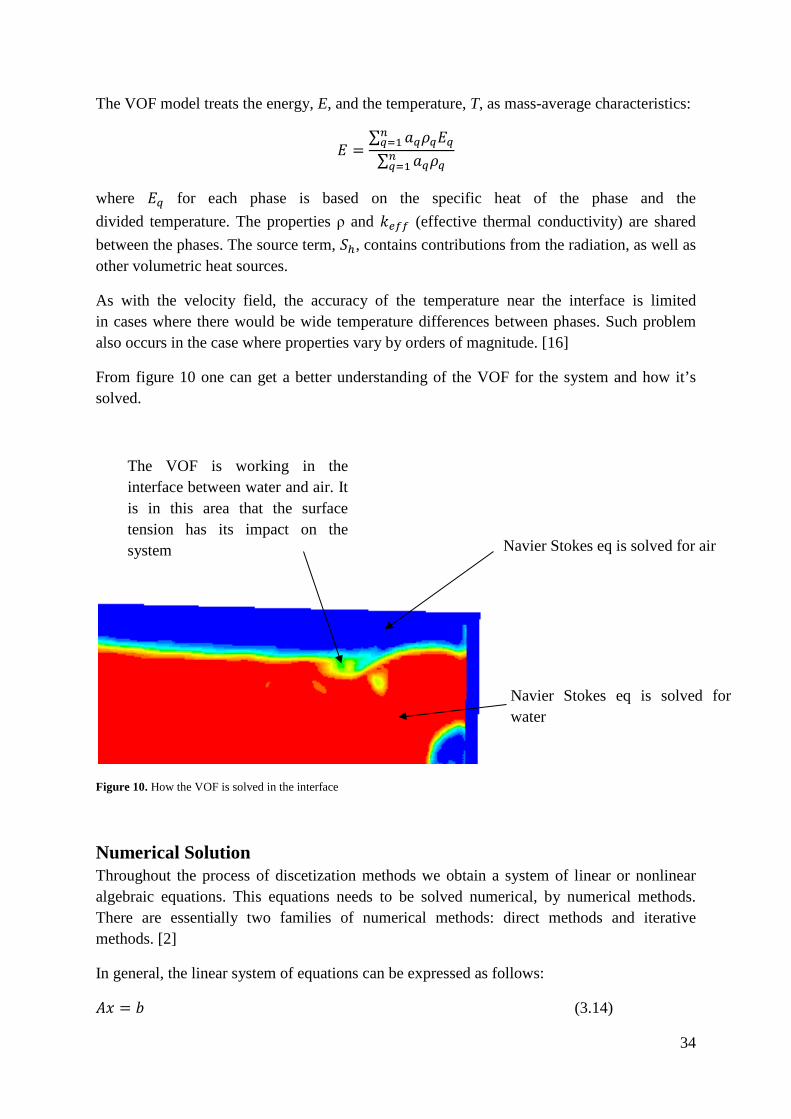
From figure 10 one can get a better understanding of the VOF for the system and how it’s solved.

Figure 10. How the VOF is solved in the interface

Numerical Solution Throughout the process of discetization methods we obtain a system of linear or nonlinear algebraic equations. This equations needs to be solved numerical, by numerical methods. There are essentially two families of numerical methods: direct methods and iterative methods. [2]

In general, the linear system of equations can be expressed as follows:

𝐴𝑥 = 𝑏 (3.14)

Navier Stokes eq is solved for air

Navier Stokes eq is solved for water

The VOF is working in the interface between water and air. It is in this area that the surface tension has its impact on the system

35

Direct/Explicit Solution Methods By definition, in an explicit approach, each difference equation contains only one unknown variable and therefore can be solved explicitly in a simple manner. [2] By explicit time marching schemes, we mean that time discretization algorithms of the coupled FSI problem is solved only once between the fluid and the structure equations within each time step. They can be typically obtained by combining an explicit algorithm for one of the subsystems (either fluid or structure) with an implicit one for the other subsystem. [6]

The Gaussian method and the triangular decomposition are two well-known methods for solving these methods.

Iterative Solution Method By definition, an implicit approach is when the unknown variable must be obtained by means of a simultaneous solution of the difference equations applied at all grid nodal points at a given time level. Implicit methods usually involve the manipulation of large matrices because of the need to solve large systems of algebraic equations.

The Jacobi method, the Gauss-Seidel method and successive over-relaxation method (SOR) are well known methods for solving stationary iterative solution methods. [2]

Consistency, Stability, Convergence and Accuracy These four words are defined as:

Consistency- A discrete approximation is said to be consistent if it approaches the original Partial Difference Equation, PDE, as ∆𝑡 and ∆𝑥 goes to zero.

Stability- A numerical solution method is considered to be stable if it does not magnify the errors that appear in the course of the numerical solution process. All errors decay so to speak.

Convergence- if a numerical method can satisfy the two important properties of consistency and stability, one generally find that the numerical procedure is convergent. Property of a numerical method to produce a solution which approaches the exact solution as the grid spacing is reduced to zero.

Accuracy- The truncation error is the difference between the discretized equation and the exact one, which gives a mean of evaluation in the accuracy of the solution for the partial differential equation.

The order of the truncation error coincides with the order of the solution error if the grid spacing are sufficiently small and if the initial and auxiliary boundary conditions are sufficiently smooth. It is commonly implied that an improvement in accuracy (from the truncation error) of high-order approximations can be achieved for a sufficient fine grid. Accuracy is usually problem dependent; an algorithm that is accurate for one model problem may not necessarily be as accurate for another more complicated problem. A converged solution does not necessarily mean a accurate solution. [2]

36

A study of added- mass effect in the design of partitioned algorithms for fluid-structure problems, made by Causin el al [6] show these results for stability in FSI :

It was observed that for these cases numerical instabilities are found:

• For a given geometry, as soon as the density of the structure is lower than a certain threshold.

• For a given structure density, as soon as the length of the domain is greater than a certain threshold.

By running the solution with “strongly” coupled methods, i.e. we ensures at each time step an exact balance of energy by sub-iterating several times between the fluid and the structure. When the subiterations consist of a relaxed fixed-point method, it was observed that an increasing amount of relaxation is needed when

• The density of the structure decreases • The length of the domain increases

The fact that numerical stability depends on the structure density has a clear physical interpretation. This is not the same for the dependence on the geometry, which is quite amazing; since the main physical phenomena is a wave propagating with a finite velocity, it is surprising that the length of the domain modifies the stability of the algorithm.

The goal is to show that explicit algorithms might be unconditionally unstable in certain cases, depending on the relative mass density of the structure and the fluid and on some geometric properties of the domain.

One conclusion that was made, for the explicit scheme, was if equation (3.15) was fulfilled the system is unconditionally unstable.

𝜌𝑠ℎ𝑠𝜌𝑓𝜇𝑚𝑎𝑥

< 1 (3.15)

where 𝜌𝑓 is the density for the fluid, 𝜌𝑠 the density for the structure, 𝜇𝑚𝑎𝑥 is the largest eigenvalue of the operator 𝑀𝐴 (se the section of FSI for definition of the operator) and ℎ𝑠 is the thickness of the structure.

Thought it appears that even when 𝜌𝑠ℎ𝑠𝜌𝑓𝜇𝑚𝑎𝑥

> 1 , that is when, for example, the structure is

much denser than the fluid, instabilities may occur if the structure is characterized by a large Young’s modulus. Nevertheless, in such a case, the scheme can be stabilized by suitable decreasing the time step.

The added mass effect, when accelerating a particle one immediately accelerates everything around it. This will end up with a system that perceived as heavier. Then equation (3.15) is approaching 1 the added mass effects get a higher impact which leads to complications in the numerical system due to the extra inertia that has been given in the system.

37

Chapter 4 Simulation and Results

FSI-simulation in ANSYS With the knowledge gained from previous work that has been done in this topic, FSI on pouring case, and with a basic model made by Tobias Berg from ANSYS Inc in Gothenburg, an ANSYS model was made and further developed to come as close to the real case as possible. The objective with the ANSYS model for FSI was to evaluate the behaviour of the pouring case and to see if we could cut down the simulation time as much as possible. To evaluate the stability for the system and what affects the different parameters in the numerical solution. One important goal was to come up with a strategy for these kinds of simulations.

The first test was, as mentioned above, the basic case implemented by Tobias Berg where the material for the model was steel with a changed Young’s modulus, which was set to 4 ∗ 108 Pa. The package in this test was smaller, 0.13 litre, than the real one litre TBA package. The surface tension was also neglected for this model. To solve the model an explicit schema was in use with a time step of 0.0005 s. Six sub iterations in Fluent was set and a boundary source coefficient of 0.065 was selected.

The tests which will be represented below are all further developments off the first model, i.e. the basic model presented above, in which some changes has been made to obtain a better understanding of FSI for the pouring case and to get as close to the real model as possible, to end up with a best practise so to speak.

All the graphs have been made in the programming software Python, where a programming script has been made. This script reads in the values of interest and plots them. The FFT for the cases of interest has also in programmed in Python with the help of the built in function fft() in Python.

Modelling The shape of the package that is studied in this thesis is simplified, since this is a basic model of the TBA-package filled with water. Hence, no seals are considered. The modelling procedure is more difficult to solve. Two models have been made for this thesis. This is due to the fact that no solution could be obtained when surface tension included, in the first model. When surface tension was switched on, it was realized that the deformation becomes bigger and a fix cap can no longer be assumed, as it gives rise to negative volumes in the deformed mesh when running the simulation. The package material is made of a linear elastic material with a Young’s modulus of initially 4*108 Pa and a density of 7500 𝑘𝑔

𝑚3.

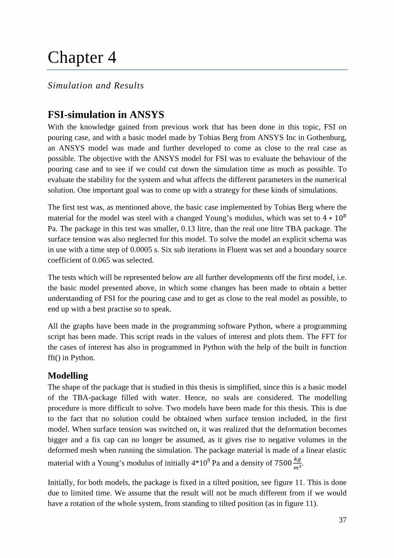
Initially, for both models, the package is fixed in a tilted position, see figure 11. This is done due to limited time. We assume that the result will not be much different from if we would have a rotation of the whole system, from standing to tilted position (as in figure 11).

38

Figure 11. Figure of the simulation of the package

The following settings have been chosen in ANSYS FLUENT for the fluid part. Finite Volume Method is used for the discretization method. The solution methods are:

Pressure-velocity coupling:

Scheme-SIMPLE

Spatial discretization:

Gradient- last squares cell bases

Pressure-PRESTO!

Momentum-bounded central differencing

Volume fraction- modified HRIC/or compressive (used both for different simulations)

The boundary conditions for the model are set to:

The shear condition is set to No slip and the wall condition is set to stationary wall for all of the package walls which are:

Wall_package_bottom, Wall_package_mx, Wall_package_mz, Wall_package_px, Wall_package_px, Wall_package_pz, Wall_package_top.

The modal analysis where done in ANSYS Mechanical by the operator modal. For solving this system the same loads as for the FSI problem was applied. The analysis was done with an

39

empty package due to the fact that one wanted to know the effect of the eigen frequencies of the package for the gulping.

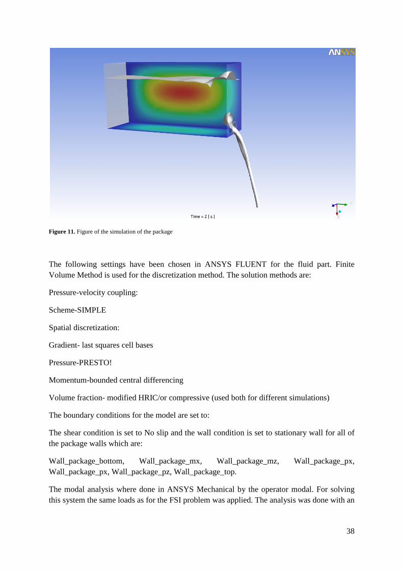
Test 1 Impact of the Boundary Source Coefficients The first test was to see how the boundary source coefficient, c, did affect the numerical stability and result of the simulation. Four values of the coefficients were tested with the values 0.07, 0.065, 0.05 and 0.03. An explicit scheme is set with a time step of 0.0005. The results of the tests are presented below.

Figure 12 shows the result of a close-up of the response graph of static pressure as a function of iterations in fluent. The red curve represent c set to 0.03, the black one set c to 0.05, yellow is set to c 0.065 and the green one is set to c as 0.07.

Figure 12. A close-up of the response graph for static pressure as a function of iterations in fluent

The result from figure 12 showed that the lowest coefficient as possible gave best convergence, and will be used as the reference values throughout the project for the test further on. The figures below, figures 13 to 16, show the results for the reference case. Figure 13 shows that the amplitude of the deformation is 0.15 mm.

40

Figure 13. Deformation in Z-direction as a function of flow time for the reference case.

Figure 14. Close-up of the response graph for static pressure average as a function of iterations in fluent for the reference case.

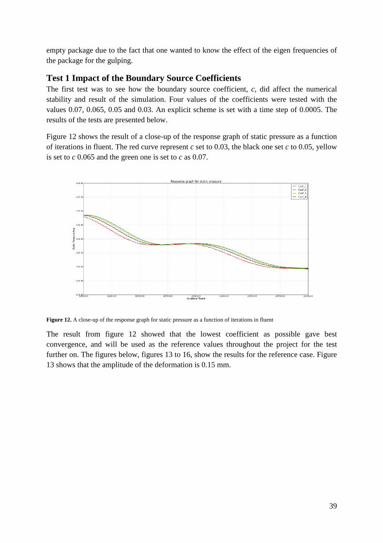
41

Figure 15. Static pressure average as a function of iterations in fluent for the reference case for the reference case.

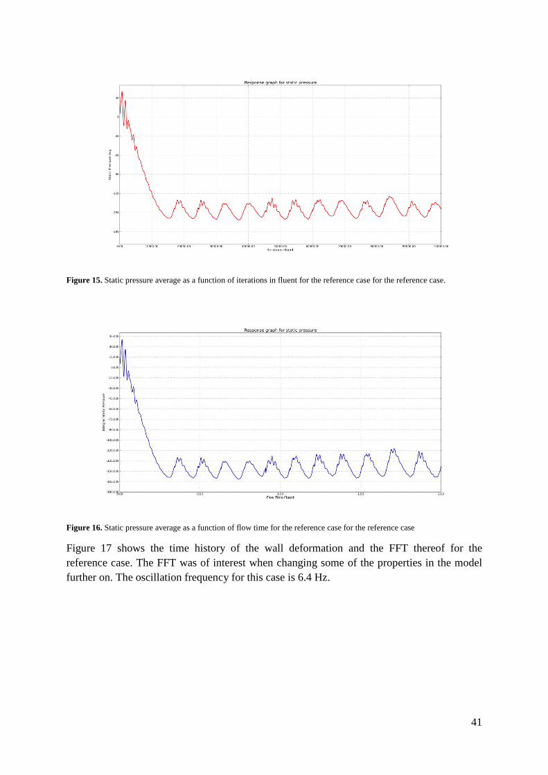
Figure 16. Static pressure average as a function of flow time for the reference case for the reference case

Figure 17 shows the time history of the wall deformation and the FFT thereof for the reference case. The FFT was of interest when changing some of the properties in the model further on. The oscillation frequency for this case is 6.4 Hz.

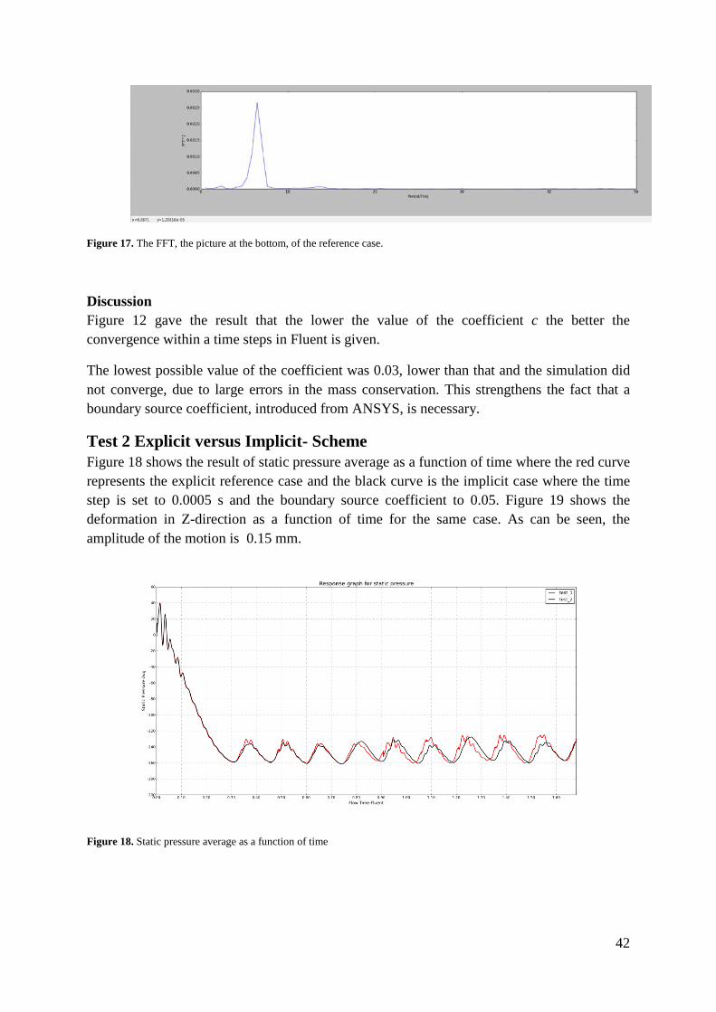
42

Figure 17. The FFT, the picture at the bottom, of the reference case.

Discussion Figure 12 gave the result that the lower the value of the coefficient c the better the convergence within a time steps in Fluent is given.

The lowest possible value of the coefficient was 0.03, lower than that and the simulation did not converge, due to large errors in the mass conservation. This strengthens the fact that a boundary source coefficient, introduced from ANSYS, is necessary.

Test 2 Explicit versus Implicit- Scheme Figure 18 shows the result of static pressure average as a function of time where the red curve represents the explicit reference case and the black curve is the implicit case where the time step is set to 0.0005 s and the boundary source coefficient to 0.05. Figure 19 shows the deformation in Z-direction as a function of time for the same case. As can be seen, the amplitude of the motion is 0.15 mm.

Figure 18. Static pressure average as a function of time

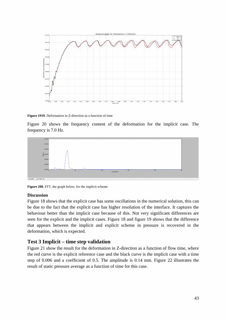
43

Figure 1919. Deformation in Z-direction as a function of time

Figure 20 shows the frequency content of the deformation for the implicit case. The frequency is 7.0 Hz.

Figure 200. FFT, the graph below, for the implicit scheme

Discussion Figure 18 shows that the explicit case has some oscillations in the numerical solution, this can be due to the fact that the explicit case has higher resolution of the interface. It captures the behaviour better than the implicit case because of this. Not very significant differences are seen for the explicit and the implicit cases. Figure 18 and figure 19 shows that the difference that appears between the implicit and explicit scheme in pressure is recovered in the deformation, which is expected.

Test 3 Implicit – time step validation Figure 21 show the result for the deformation in Z-direction as a function of flow time, where the red curve is the explicit reference case and the black curve is the implicit case with a time step of 0.006 and a coefficient of 0.5. The amplitude is 0.14 mm. Figure 22 illustrates the result of static pressure average as a function of time for this case.

44

Figure 21. Deformation in Z-direction as a function of flow time

Figure 22. Static pressure average as a function of flow time

Figure 23 shows a close-up of the response graph for static average pressure as a function of iterations in fluent. Time step is set to 0.004 s with c = 0.08 with a compressive solver for the VOF.

45

Figure 213. Close-up of the response graph for static pressure average as a function of iterations in fluent

Figure 24 shows the static pressure for the implicit scheme with a time step of 0.006 s and a boundary source coefficient of 0.05.

Figure 28. Close-up of the response graph for static pressure average as a function of iterations in fluent

Figure 25 show the frequency spectrum, for the deformation, for the implicit case for the time step 0.006 and boundary source coefficient set to 0.05. The value of the frequency is 6.6 Hz.

46

Figure 225. FFT, the graph below, for the implicit scheme

Discussion Increasing the time step size, which is a necessary criterion for Tetra Pak to lower the simulation time, for a converged solution was only obtained with the implicit scheme. It was possible to increase the time step size by a factor 12.

By looking at the FFT for both cases, implicit and explicit, one realise that the frequency is the same for the explicit case and for the implicit case, which strengthen the argument for running implicit scheme more.

The larger the time step the larger boundary source coefficient is needed. It’s a trade of between time and accuracy.

By looking at figures 21 and 22 we see that a twelve times larger time step gives an acceptable result with a much faster solution. The difference in the result ought to be that the larger time step, results in loss of information in wave propagation due to too large time step will introduce implicit spatial filtering.

By having the time step set to 0.0005 s and run to 0.24 seconds it takes 6 hours. A simulation with a time step of 0.006 s run in 2.88 seconds takes 14.4 hours to run. This means that it takes 25 hours to run 1 second for the time step 0.0005 but just 5 hours to run 1 second with a time step set to 0.006 s. We have got a solution which is 5 times faster. Both cases are run with 60 cores. This is representative result for a small package, for a larger package computational power will be increased.

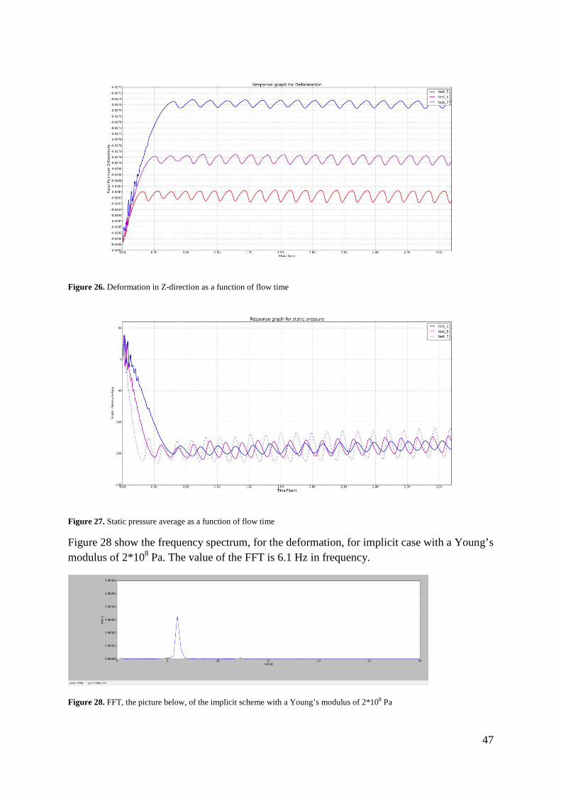
Test 4 Young’s modulus Figure 26 show the response graph for deformation in Z-direction as a function of time for the implicit scheme with a time step of 0.006 and a coefficient of 0.05. All three cases have more or less the same amplitude, which is 0.1 mm. Figure 27 shows the result of static pressure average as a function of time for the same case. In test 5 the Young’s modulus has a value of 2 ∗ 108 , in test 6 the value is 4 ∗ 108 and for test 7 the modulus is 8 ∗ 108.

47

Figure 26. Deformation in Z-direction as a function of flow time

Figure 27. Static pressure average as a function of flow time

Figure 28 show the frequency spectrum, for the deformation, for implicit case with a Young’s modulus of 2*108 Pa. The value of the FFT is 6.1 Hz in frequency.

Figure 28. FFT, the picture below, of the implicit scheme with a Young’s modulus of 2*108 Pa

48

Discussion The larger the Young’s modulus for the package material, the higher the static pressure is in the package, which can also relate to the deformation and shows that the package has smaller contraction for higher values.

If we take a look at figure 26, which shows the deformation, we realize that the amplitudes for the three cases are very similar, although the Young’s modulus differs for each one of them. This should make the pressure different, such that the one with highest Young’s modulus should have the highest pressure. By looking at figure 27 we state that this is correct.

The conclusion of this is that for any chosen Young’s modulus in this interval will not have an impact on the gulping frequency or amplitude.

Test 5 Density validation Figure 29 shows the response graph for deformation in Z-direction as a function of the flow time for the implicit coupling algorithm with a time step of 0.006 s and a boundary source coefficient of 0.065. The green curve shows the result for a density set to 𝜌 = 7500 𝑘𝑔

𝑚3 and

the blue graph has the density 𝜌 = 2000 𝑘𝑔𝑚3. The Young’s modulus is set to 𝐸 = 2 ∗ 108 𝑃𝑎.

The purple curve have a density set to 𝜌 = 800 𝑘𝑔𝑚3 and a Young’s modulus of 𝐸 = 2 ∗

108 𝑃𝑎, the coefficient is set to 0.15. All curves have more or less the same amplitude, which is 0.1 mm. Figure 30 illustrates the result for static pressure average as a function of flow time for the same case.

Figure 29. Deformation in Z-direction as a function of flow time

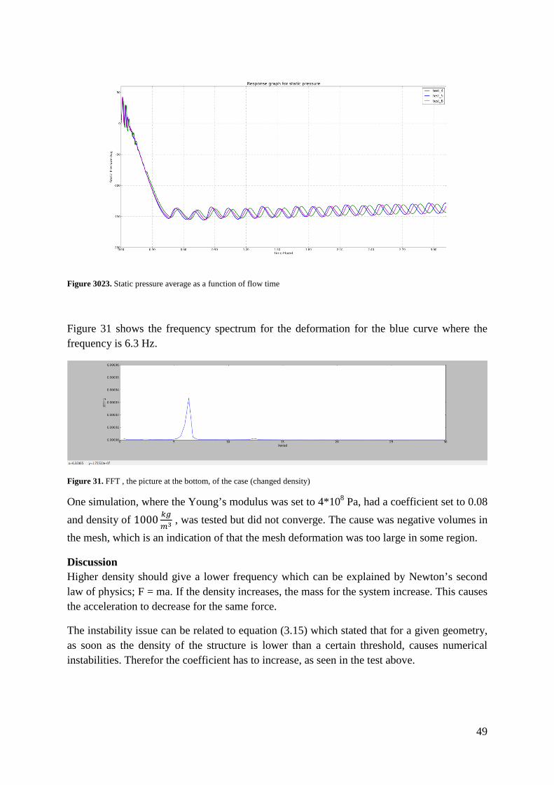
49

Figure 3023. Static pressure average as a function of flow time

Figure 31 shows the frequency spectrum for the deformation for the blue curve where the frequency is 6.3 Hz.

Figure 31. FFT , the picture at the bottom, of the case (changed density)

One simulation, where the Young’s modulus was set to 4*108 Pa, had a coefficient set to 0.08 and density of 1000 𝑘𝑔

𝑚3 , was tested but did not converge. The cause was negative volumes in the mesh, which is an indication of that the mesh deformation was too large in some region.

Discussion Higher density should give a lower frequency which can be explained by Newton’s second law of physics; F = ma. If the density increases, the mass for the system increase. This causes the acceleration to decrease for the same force.

The instability issue can be related to equation (3.15) which stated that for a given geometry, as soon as the density of the structure is lower than a certain threshold, causes numerical instabilities. Therefor the coefficient has to increase, as seen in the test above.

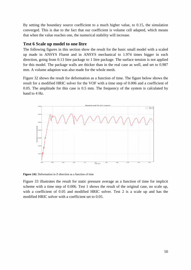
50

By setting the boundary source coefficient to a much higher value, to 0.15, the simulation converged. This is due to the fact that our coefficient is volume cell adapted, which means that when the value reaches one, the numerical stability will increase.

Test 6 Scale up model to one litre The following figures in this section show the result for the basic small model with a scaled up made in ANSYS Fluent and in ANSYS mechanical to 1.974 times bigger in each direction, going from 0.13 litre package to 1 litre package. The surface tension is not applied for this model. The package walls are thicker than in the real case as well, and set to 0.987 mm. A volume adaption was also made for the whole mesh.

Figure 32 shows the result for deformation as a function of time. The figure below shows the result for a modified HRIC solver for the VOF with a time step of 0.006 and a coefficient of 0.05. The amplitude for this case is 0.5 mm. The frequency of the system is calculated by hand to 4 Hz.

Figure 242. Deformation in Z-direction as a function of time

Figure 33 illustrates the result for static pressure average as a function of time for implicit scheme with a time step of 0.006. Test 1 shows the result of the original case, no scale up, with a coefficient of 0.05 and modified HRIC solver. Test 2 is a scale up and has the modified HRIC solver with a coefficient set to 0.05.

51

Figure 33. Static pressure average as a function of time

Discussion Figures 32 and 33 shows that the result of a scale up is possible to simulate and be able to converge, without numerical difficulties. To run this case with surface tension was not possible and therefore model 2 was made, which is presented below in test 7.

Test 7 surface tension on one litre package Test 6 did not converge with surface tension and there for a new model was made. This model has got more grids than the other one and the cap is not fixed as for the old model. To be able to compare the results with Test 6, two models have been tested in this case - one with a thicker wall of the package, the same as for Test 6, 0.987 mm. The other one has a wall thickness of 0.5 mm. This was made because of the fact when a scale up was made in test 6 the walls also got thicker. We want to compare test 7 with test 6, but also come closer to the “real” TBA package (which has a wall thickness of 0.5 mm), and there for two models where tested. The surface tension is set to 0.072 N/m in ANSYS fluent and the Wall Adhesion to 90 degree for x+, y+ and z+. The Young’s modulus is set to 4*108 Pa.

Thicker wall: The response graphs below show the result of an implicit scheme with a compressive scheme for the VOF. The green curve has a time step of 0.004 s and a boundary source coefficient of 0.1. The blue curve has a time step of 0.002 and a coefficient of 0.05. The purple one a time step of 0.002 and a coefficient of 0.08. Figure 34 illustrates the deformation in Z-direction as a function of time whereas figure 35 shows the deformation in X-direction as a function of time. The static pressure average as a function of time is shown in figure 36 and close-up of figure 36 is seen in figure 37. The amplitude, for the deformation in Z-direction, for the three cases is 0.4 mm.

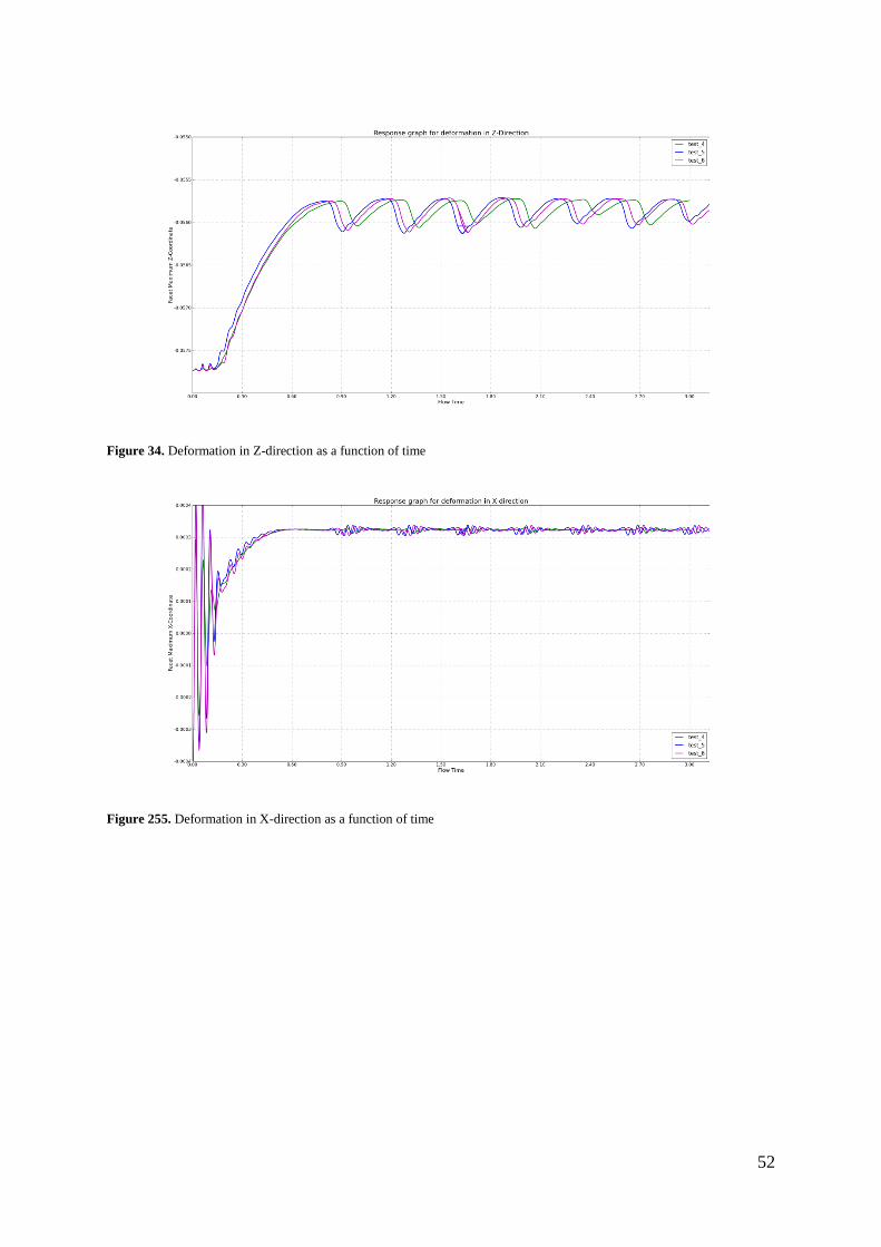
52

Figure 34. Deformation in Z-direction as a function of time

Figure 255. Deformation in X-direction as a function of time

53

Figure 36. Static pressure average as a function of time

Figure 3726. Close up of static pressure average as a function of iterations in fluent

Figure 38 shows the frequency content of the deformation in Z-direction for the thicker wall with a time step of 0.004 and a coefficient of 0.1. The frequency is 1.9 Hz.

Figure 3827. FFT, figure at the bottom, of the case with a time step set to 0.004 and a coefficient set to 0.1

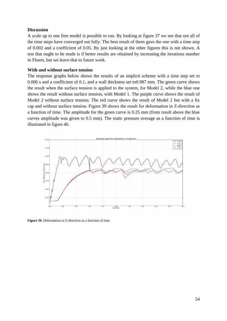
54

Discussion A scale up to one litre model is possible to run. By looking at figure 37 we see that not all of the time steps have converged out fully. The best result of them gave the one with a time step of 0.002 and a coefficient of 0.05. By just looking at the other figures this is not shown. A test that ought to be made is if better results are obtained by increasing the iterations number in Fluent, but we leave that to future work.

With and without surface tension The response graphs below shows the results of an implicit scheme with a time step set to 0.006 s and a coefficient of 0.1, and a wall thickness set to0.987 mm. The green curve shows the result when the surface tension is applied to the system, for Model 2, while the blue one shows the result without surface tension, with Model 1. The purple curve shows the result of Model 2 without surface tension. The red curve shows the result of Model 2 but with a fix cap and without surface tension. Figure 39 shows the result for deformation in Z-direction as a function of time. The amplitude for the green curve is 0.25 mm (from result above the blue curves amplitude was given to 0.5 mm). The static pressure average as a function of time is illustrated in figure 40.

Figure 39. Deformation in Z-direction as a function of time

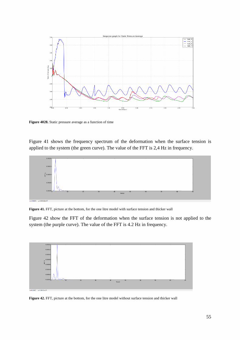
55

Figure 4028. Static pressure average as a function of time

Figure 41 shows the frequency spectrum of the deformation when the surface tension is applied to the system (the green curve). The value of the FFT is 2,4 Hz in frequency.

Figure 41. FFT, picture at the bottom, for the one litre model with surface tension and thicker wall

Figure 42 show the FFT of the deformation when the surface tension is not applied to the system (the purple curve). The value of the FFT is 4.2 Hz in frequency.

Figure 42. FFT, picture at the bottom, for the one litre model without surface tension and thicker wall

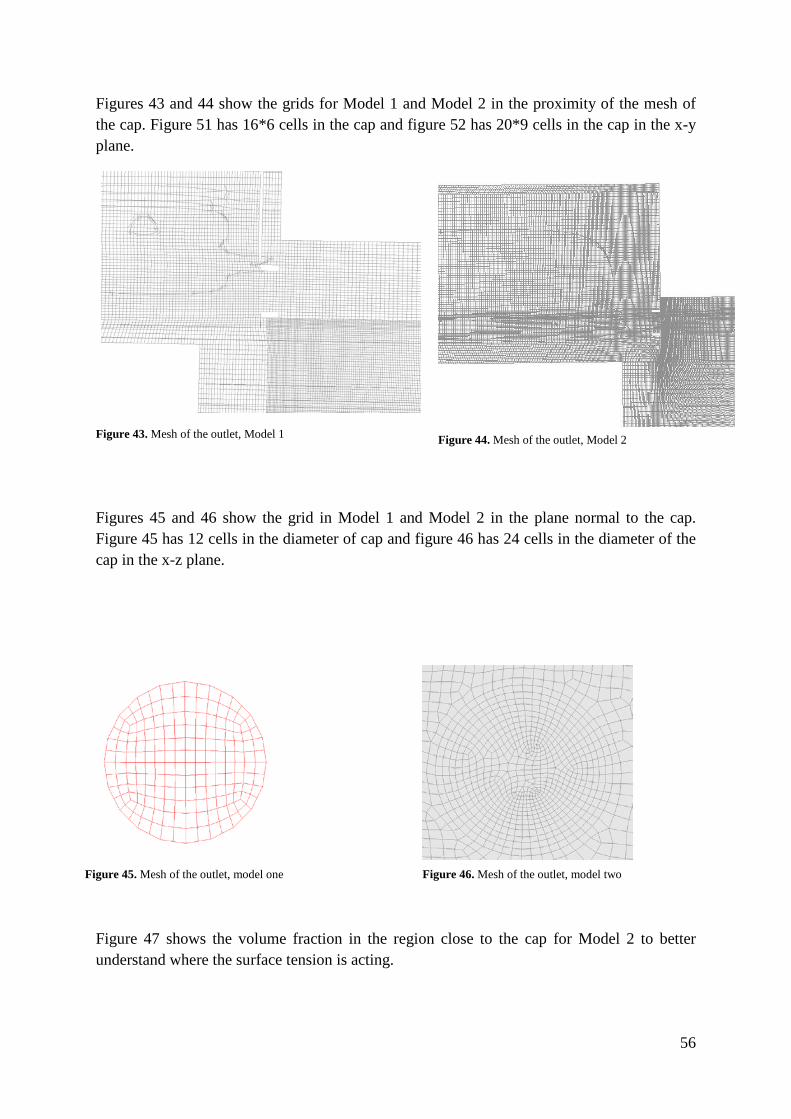
56

Figures 43 and 44 show the grids for Model 1 and Model 2 in the proximity of the mesh of the cap. Figure 51 has 16*6 cells in the cap and figure 52 has 20*9 cells in the cap in the x-y plane.

Figure 43. Mesh of the outlet, Model 1

Figures 45 and 46 show the grid in Model 1 and Model 2 in the plane normal to the cap. Figure 45 has 12 cells in the diameter of cap and figure 46 has 24 cells in the diameter of the cap in the x-z plane.

Figure 47 shows the volume fraction in the region close to the cap for Model 2 to better understand where the surface tension is acting.

Figure 44. Mesh of the outlet, Model 2

Figure 45. Mesh of the outlet, model one Figure 46. Mesh of the outlet, model two

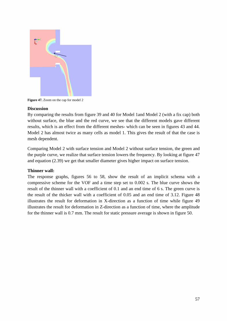
57

Figure 47. Zoom on the cap for model 2

Discussion By comparing the results from figure 39 and 40 for Model 1and Model 2 (with a fix cap) both without surface, the blue and the red curve, we see that the different models gave different results, which is an effect from the different meshes- which can be seen in figures 43 and 44. Model 2 has almost twice as many cells as model 1. This gives the result of that the case is mesh dependent.

Comparing Model 2 with surface tension and Model 2 without surface tension, the green and the purple curve, we realize that surface tension lowers the frequency. By looking at figure 47 and equation (2.39) we get that smaller diameter gives higher impact on surface tension.

Thinner wall: The response graphs, figures 56 to 58, show the result of an implicit schema with a compressive scheme for the VOF and a time step set to 0.002 s. The blue curve shows the result of the thinner wall with a coefficient of 0.1 and an end time of 6 s. The green curve is the result of the thicker wall with a coefficient of 0.05 and an end time of 3.12. Figure 48 illustrates the result for deformation in X-direction as a function of time while figure 49 illustrates the result for deformation in Z-direction as a function of time, where the amplitude for the thinner wall is 0.7 mm. The result for static pressure average is shown in figure 50.

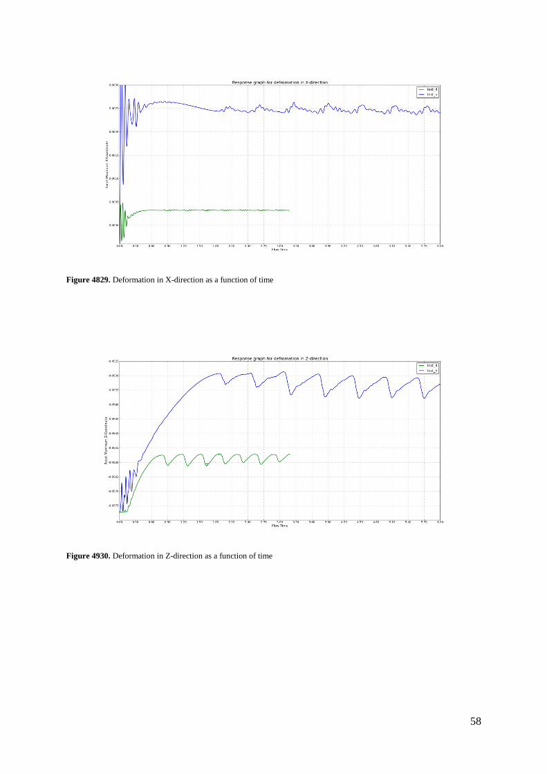
58

Figure 4829. Deformation in X-direction as a function of time

Figure 4930. Deformation in Z-direction as a function of time

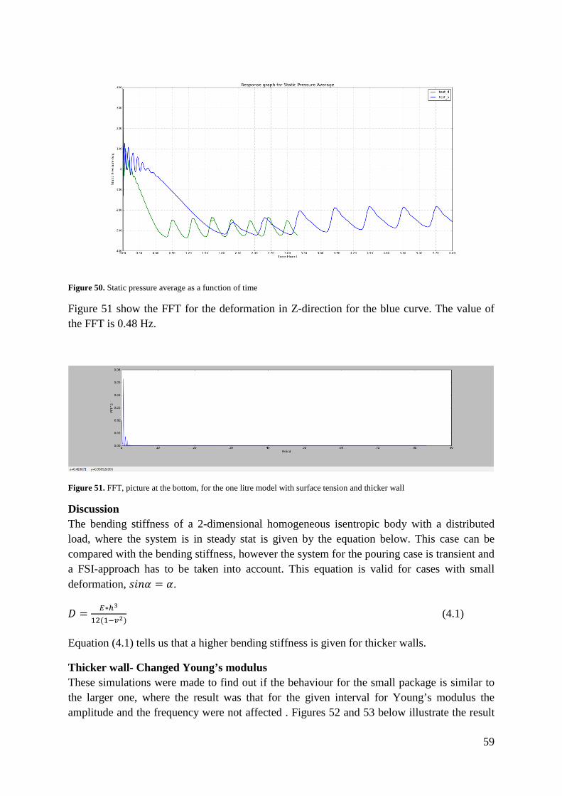
59

Figure 50. Static pressure average as a function of time

Figure 51 show the FFT for the deformation in Z-direction for the blue curve. The value of the FFT is 0.48 Hz.

Figure 51. FFT, picture at the bottom, for the one litre model with surface tension and thicker wall

Discussion The bending stiffness of a 2-dimensional homogeneous isentropic body with a distributed load, where the system is in steady stat is given by the equation below. This case can be compared with the bending stiffness, however the system for the pouring case is transient and a FSI-approach has to be taken into account. This equation is valid for cases with small deformation, 𝑠𝑖𝑛𝛼 = 𝛼.

𝐷 = 𝐸∗ℎ3

12(1−𝑣2) (4.1)

Equation (4.1) tells us that a higher bending stiffness is given for thicker walls.

Thicker wall- Changed Young’s modulus These simulations were made to find out if the behaviour for the small package is similar to the larger one, where the result was that for the given interval for Young’s modulus the amplitude and the frequency were not affected . Figures 52 and 53 below illustrate the result

60

for model 2, one litre package with thicker wall, density set to 7500 𝑘𝑔𝑚3 , time step of 0.006

and a boundary source coefficient of 0.1. The red curve has a Young’s modulus set to 4*108 Pa and the black curve has the value of 8*108 Pa. Figure 52 shows the deformation in Z-direction as a function of time while figure 53 illustrates the result for static pressure average as a function of time for the same case.

Figure 52. Deformation in Z-direction as a function of time

Figure 5331. Static pressure average as a function of time

Figure 54 show the FFT for the deformation in Z-direction for the black curve. The value of the FFT is 4.4 Hz.

61

Figure 54. FFT, picture at the bottom, for the one litre model without surface tension, Young’s modulus 8*108 Pa and thicker wall

Discussion Young’s modulus does not have an impact on the frequency for Model 2 for the given interval. The amplitude is little affected by the change in Young’s modulus, where a Young’s modulus set to 4*108 Pa gives an amplitude difference of 3*10-4 and a Young’s modulus set to 8*108 Pa gives an amplitude difference of 2*10-4.

Test 8 Module Analysis The figures below show the result for the module analysis that was made in ANSYS Mechanical, modal. In figure 55 the Young’s modulus is set to 4*108 Pa and had a density of 7500 𝑘𝑔

𝑚3, whereas in figure 56, for the same Young’s modulus, the density is set to 800 𝑘𝑔𝑚3.

Figure 57 illustrates the result for the module analysis for a Young’s modulus set to 2*108 Pa and had a density of 800 𝑘𝑔

𝑚3. Please note that no effect of water was considered.

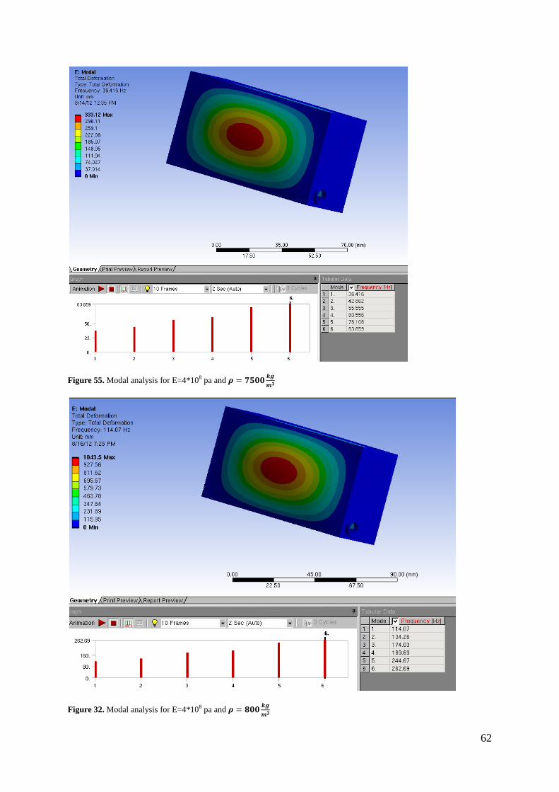
62

Figure 55. Modal analysis for E=4*108 pa and 𝝆 = 𝟕𝟓𝟎𝟎 𝒌𝒈𝒎𝟑

Figure 32. Modal analysis for E=4*108 pa and 𝝆 = 𝟖𝟎𝟎 𝒌𝒈𝒎𝟑

63

Figure 57. Modal analysis for E=2*108 pa and 𝝆 = 𝟖𝟎𝟎 𝒌𝒈𝒎𝟑

Discussion The modal analysis gives the result of that the amplitude and the frequency that is given for the FSI problem is not effected of the eigenvalues of an empty package.

The modal analysis is performed on an empty package, i.e. the results obtained are the in vacou eigenfrequencies. This means that the effect of added mass in the eigenfrequencies is not accounted for. However, even though the added mass effect would lower the eigenfrequencies somewhat they would still be, for the geometries considered, consideranbly higher than the frequencies obtained for the gulping. Hence, one may assume that the eigenmodes of the package does not influence the gulping frequency.

The result in the figures 55 to 57 shows that the lower the density for the system the higher the eigenfrequencies will be. This can be related for the equation for the beam, where the eigenfrequency is given by:

𝑓𝑛 ∝ �𝐸𝜌 (4.2)

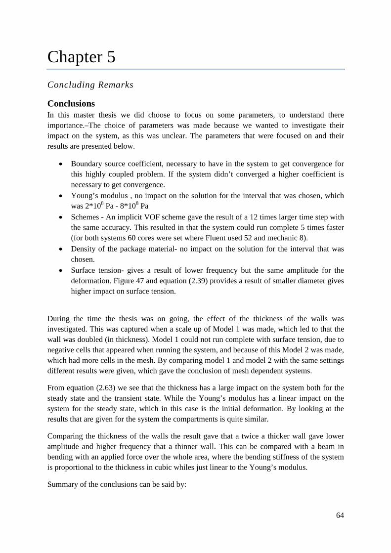
64

Chapter 5 Concluding Remarks

Conclusions In this master thesis we did choose to focus on some parameters, to understand there importance. The choice of parameters was made because we wanted to investigate their impact on the system, as this was unclear. The parameters that were focused on and their results are presented below.

• Boundary source coefficient, necessary to have in the system to get convergence for this highly coupled problem. If the system didn’t converged a higher coefficient is necessary to get convergence.

• Young’s modulus , no impact on the solution for the interval that was chosen, which was 2*108 Pa - 8*108 Pa

• Schemes - An implicit VOF scheme gave the result of a 12 times larger time step with the same accuracy. This resulted in that the system could run complete 5 times faster (for both systems 60 cores were set where Fluent used 52 and mechanic 8).

• Density of the package material- no impact on the solution for the interval that was chosen.

• Surface tension- gives a result of lower frequency but the same amplitude for the deformation. Figure 47 and equation (2.39) provides a result of smaller diameter gives higher impact on surface tension.

During the time the thesis was on going, the effect of the thickness of the walls was investigated. This was captured when a scale up of Model 1 was made, which led to that the wall was doubled (in thickness). Model 1 could not run complete with surface tension, due to negative cells that appeared when running the system, and because of this Model 2 was made, which had more cells in the mesh. By comparing model 1 and model 2 with the same settings different results were given, which gave the conclusion of mesh dependent systems.

From equation (2.63) we see that the thickness has a large impact on the system both for the steady state and the transient state. While the Young’s modulus has a linear impact on the system for the steady state, which in this case is the initial deformation. By looking at the results that are given for the system the compartments is quite similar.

Comparing the thickness of the walls the result gave that a twice a thicker wall gave lower amplitude and higher frequency that a thinner wall. This can be compared with a beam in bending with an applied force over the whole area, where the bending stiffness of the system is proportional to the thickness in cubic whiles just linear to the Young’s modulus.

Summary of the conclusions can be said by:

65

• Success with FSI in ANSYS for a conceptual pouring application due to the fact that the case did run complete

• With the help of the boundary source coefficient we are able to perform strong coupled systems for the pouring application

• FSI coupling has proven robust through different challenging process, by changing density ratios, Young’s modulus, thickness of the wall, package volume

• There are strong indications that the geometry and design have a large impact in the result, while the material properties have less impact on gulping

• With given parameters such as Young’s modulus and density expected results can be made in regarding the gulping of the package.

66

Summary Table 2 shows a summary of all the tests that have been made for frequency and the amplitude that were given for the tests, from the deformation in Z-direction. The Young’s modulus is a factor of x*108 Pa.

Table 1. Summary of the tests made for frequency and amplitude

Future work By having worked with this thesis we realize how much interest Tetra Pak has to retrieve in this topic, FSI in pouring application. This also opens doors for further development, jobs and further master thesis. This thesis is in the interface between numerical models and the real case for the pouring application, and the next step for future work might be:

• Recreate validation pouring case to validate with experimental data • A deeper understanding of the material and egenvalues for the structure • Possible to derive analytical expression for pouring • Next step is to take the model further on to the real pouring application

67

Chapter 6

Reference [1] Young, D. F., Munson, B. R., Okiishi, T. H., Huebsch, W. W.: Introduction to Fluid Mechanics, 5th Edition (SI Version). John Wiley & Sons, 2012, ISBN: 978-0-470-90215-8

[2] Tu, Heng Yeoh, Liu : Computational Fluid Dynamics, A Practical Approach; First edition, Butterworth-Heinemann, 2008 ; ISBN: 978-0-7506-8563-4

[3] Stephen B. Pope : Turbulent Flows ; Cambridge University Press, 2000

[4] Krenk, Steen : Non-linear Modeling and Analysis of Solids and Structures ; First Editon 2009, ISBN: 978-0-521-83054-6

[5] O.C. Zienkiewicz & R.L. Taylor The Finite Element Method, Volume II. Butterworth Heinemann, Fith Edition, 2000.

[6] Causin P, Gerbeau J-F and Nobile Fabio : Added- mass effect in the design of partitioned algorithms for fluid-structure problems ; INRIA Rocquencourt, No5084 Janvier 2004

[7] Nygårds Mikael : Modelling and simulation of paperboard damage and deformation-Executive summaty of the Liquid Paperboard Cluster ; Innventia Report No.:45 December 2009

[8] Shyy Wei : Transport processes in engineering, 5. Computational modelling of fluid flow and interfacial transport ; department of aerospace Engineering, Mechanics and Engineering Science, University of Florida, Gainesville, FL 32611, USA, ELSEVIER

[9] Article provided by Ansys Inc in Gothenburg

[10] http://www.ansys.com/Products

[11] http://en.wikipedia.org/wiki/Ansys

[12] N.S. Ottosen, H. Petterson, “Introduction to Finite Element Method”, PEARSON, Prentice Hall, 1992

[13] http://www.tetrapak.com , Product images

[14] Sundén Bengt, Eriksson Daniel, Yuan Jinliang : Introduction to NUMERICAL HEAT TRANSFER ; Lunds Universitet, Division of heat transfer, Department of Energy Sciencse, August 2010

[15] Vinay R. Gopala : Modeling of Interfacial Flows with Mass-Transfer; Department of Applied Mechanics, Chalmers Univeristy of Technology, Göteborg, Sweden 2008

[16] ANSYS User Guide-Theory Guide- Multiphase Flows

68

[17] The Fast Fourier Transform (FFT); Springer Series in Optical Sciences, 2008, Volume 35, Engineering Optics, Pages 161-179

[18] http://en.wikipedia.org/wiki/Fast_Fourier_transform

[19] http://en.wikipedia.org/wiki/Modal_analysis

[20] Tony L. Schmitz and Kevin S. Smith, Modal Analysis, 2009, Machining Dynamics, Pages 7-57