Fluid Mechanics

Chapter 5 Control Volume Approach and

Continuity Equation

Dr. Amer Khalil Ababneh

Approach to Analyses of Fluid flows

The engineer can find flow properties (pressure and velocity) in a

flow field in one of two ways. One approach is to generate a

series of pathlines or streamlines through the field and

determine flow properties at any point along the lines by

applying equations like those developed in Chapter 4. This is

called the Lagrangian approach. The other way is to solve a

set of equations for flow properties at any point in the flow field.

This is called the Eulerian approach (also called control

volume approach).

The foundational concepts for the Eulerian approach, or control

volume approach, are developed and applied to the

conservation of mass. This leads to the continuity equation, a

fundamental and widely used equation in fluid mechanics.

Control volume is a region in space that allows mass to flow in

and out of it.

5.1 Rate of Flow It is necessary to be able to calculate the flow rates

through a control volume. Also, the capability to calculate flow rates is important in analyzing water supply systems, natural gas distribution networks, and river flows.

Discharge The discharge, Q, often called the volume flow rate, is

the volume of fluid that passes through an area per unit time. For example, when filling the gas tank of an automobile, the discharge or volume flow rate would be the gallons per minute flowing through the nozzle. Typical units for discharge are ft3/s (cfs), ft3/min (cfm), gpm, m3/s, and L/s.

Figure 5.3 Volume of fluid in flow with uniform velocity distribution that passes section A-A in time t.

To develop an equation for the discharge, consider a fluid flow

with a uniform velocity flowing in a pipe, Figure 5.3. The volume of

the fluid indicated that passes section A-A is during time interval Dt

D = A Dl = A (V Dt)

The volume flow rate is the volume indicated per unit time

Taking the limit as Dt → 0 gives

=Dl

Volume flow rate is referred to as discharge and will be given the

symbol Q.

In general the velocity is not uniform and in this case the

discharge is given by

The mean velocity is defined as the discharge divided by the

cross-sectional area,

For laminar flows in circular pipes, the velocity profile is parabolic,

and the mean velocity is half the centerline velocity. For turbulent

pipe flow time-averaged velocity profile is nearly uniformly

distributed across the pipe, so the mean velocity is fairly close to

the velocity at the pipe center. It is customary to leave the bar off

the velocity symbol and simply indicate the mean velocity with V.

In Fig. 5.5 the flow velocity vector is not normal to the surface but

is oriented at an angle θ with respect to the direction that is

normal to the surface. The only component of velocity that

contributes to the flow through the differential area dA is the

component normal to the area, Vn. The differential discharge

through area dA is

Figure 5.5 Velocity vector oriented at angle θ with respect to normal.

dAVdQn

=

Note that the dA is a vector with magnitude and direction normal

to the area. But since Vn dA = abs(V) cos(q) dA = V.dA, then in

general, the discharge is

If the velocity is uniform, the discharge is

Note, if the velocity is tangent to the surface area, then the

discharge is zero.

Mass Flow Rate

The mass flow rate, , is the mass of fluid passing through a

cross-sectional area per unit time. The common units for mass

flow rate are kg/s, lbm/s, and slugs/s. Using the same approach

as for volume flow rate, the mass of the fluid in the marked

volume in Fig. 5.3 is , where ρ is the average

density. The mass flow rate equation is

m

As before in case of discharge, the general form of mass flow

rate is

The mass flow rate also can be expressed in terms of the mean

velocity as,

EXAMPLE 5.1 VOLUME FLOW RATE AND MEAN

VELOCITY

Air that has a mass density of 1.24 kg/m3 flows in a pipe with a

diameter of 30 cm at a mass rate of flow of 3 kg/s. What are

the mean velocity and discharge in this pipe?

Solution

1. Discharge:

2. Mean velocity

EXAMPLE 5.2 FLOW IN SLOPING CHANNEL

Water flows in a channel that has a slope of 30°. If the velocity is

assumed to be constant, 12 m/s, and if a depth of 60 cm is

measured along a vertical line, what is the discharge per meter

of width of the channel?

Solution

EXAMPLE 5.3 DISCHARGE IN CHANNEL WITH NON-

UNIFORM VELOCITY DISTRIBUTION

The water velocity in the channel shown in the accompanying figure

has a distribution across the vertical section equal to u/umax =

(y/d)1/2. What is the discharge in the channel if the water is 2 m

deep (d = 2 m), the channel is 5 m wide, and the maximum

velocity is 3 m/s?

Solution

The discharge equation,

5.2 Control Volume Approach

The control volume (or Eulerian) approach is the method whereby a volume in the flow field is identified and the governing equations are solved for the flow properties associated with this volume. A scheme is needed that allows one to rewrite the equations for a moving fluid particle in terms of flow through a control volume. Such a scheme is the Reynolds transport theorem.

Definition: System and Control Volume

A system is a continuous mass of fluid that always contains the same matter. A system moving through a flow field is shown in Fig. 5.6. The shape of the system may change with time, but the mass is constant since it always consists of the same matter. The fundamental equations, such as Newton's second law and the first law of thermodynamics, apply to a system.

Figure 5.6 System, control surface, and control volume in a flow field.

A control volume is volume located in space and through which matter

can pass, as shown in Fig. 5.6. The indicated system can pass through

the control volume. The selection of the control volume position and

shape is problem dependent. The control volume is enclosed by the

control surface as shown in Fig. 5.6. Fluid mass enters and leaves the

control volume through the control surface. The control volume can

deform with time as well as move and rotate in space and the mass in

the control volume can change with time.

Intensive and Extensive Properties

An extensive property is any property that depends on the amount of matter present. The extensive properties of a system include mass, m, momentum, mv (where v is velocity), and energy, E. Another example of an extensive property is weight because the weight is mg. An intensive property is any property that is independent of the amount of matter present. Examples of intensive properties include pressure and temperature. Many intensive properties are obtained by dividing the extensive property by the mass present. The intensive property for momentum is velocity v, and for energy is e, the energy per unit mass. The intensive property for weight is g.

In this section an equation for a general extensive property, B, will be developed. The corresponding intensive property will be b. The amount of extensive property B contained in a control volume at a given instant is

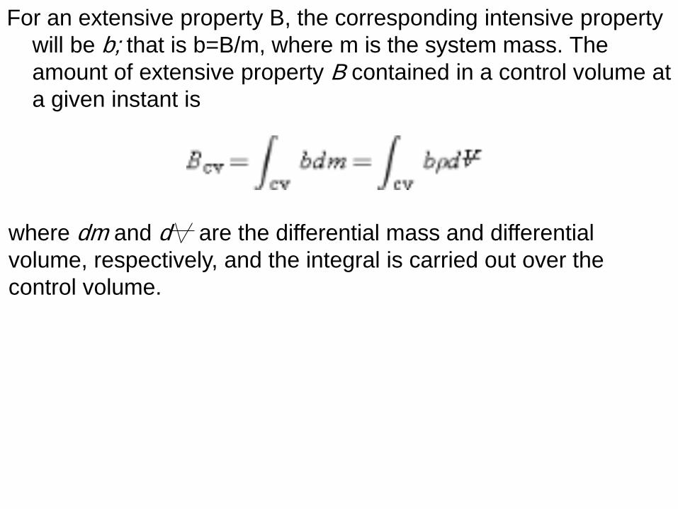
For an extensive property B, the corresponding intensive property

will be b; that is b=B/m, where m is the system mass. The

amount of extensive property B contained in a control volume at

a given instant is

where dm and d are the differential mass and differential

volume, respectively, and the integral is carried out over the

control volume.

Property Transport Across the Control Surface

When fluid flows across a control surface, properties such as mass, momentum, and energy are transported with the fluid either into or out of the control volume. Consider the flow through the control volume in the duct in Fig. 5.7. If the velocity is uniformly distributed across the control surface, the mass flow rate through each cross section is given by

Figure 5.7 Flow through control volume in a duct.

The net mass flow rate out* of the control volume, that is, the

outflow rate minus the inflow rate, is

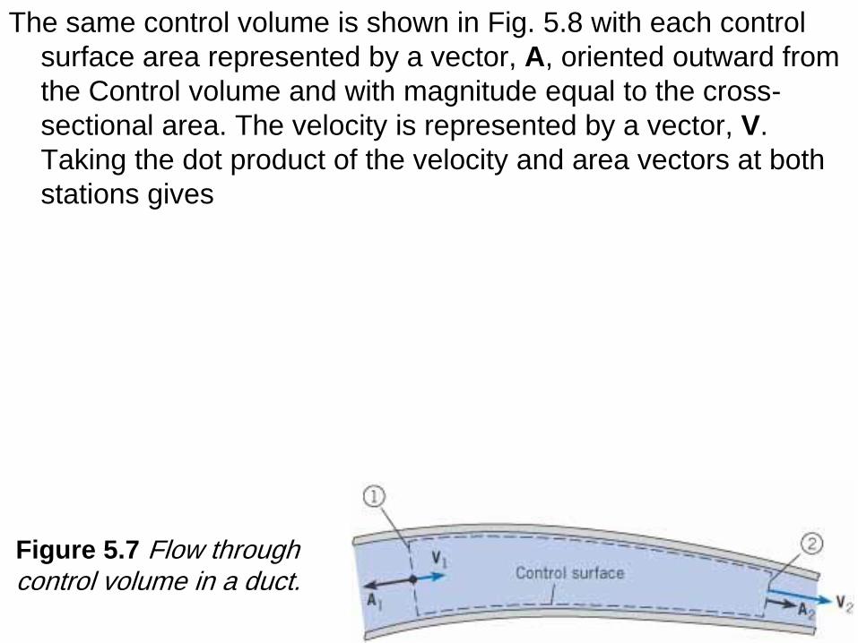
The same control volume is shown in Fig. 5.8 with each control

surface area represented by a vector, A, oriented outward from

the Control volume and with magnitude equal to the cross-

sectional area. The velocity is represented by a vector, V.

Taking the dot product of the velocity and area vectors at both

stations gives

Figure 5.7 Flow through control volume in a duct.

Because at station 1 the velocity and area have the opposite directions while at station 2 the velocity and area vectors are in the same direction. Now the net mass outflow rate can be written a

(5.11)

Equation (5.11) states that if the dot product ρV · A is summed for

all flows into and out of the control volume, the result is the net

mass flow rate out of the control volume, or the net mass efflux. If

the summation is positive, the net mass flow rate is out of the

control volume. If it is negative, the net mass flow rate is into the

control volume. If the inflow and outflow rates are equal, then

there is no change of mass inside the control volume.

Similarly, to obtain the net rate of flow of an extensive property B out of the control volume, the mass flow rate is multiplied by the

intensive property b:

(5.12)

Equation (5.12) is applicable for all flows where the properties are

uniformly distributed across the area. If the properties vary across

a flow section, then it becomes necessary to integrate across the

section to obtain the rate of flow. Specifically,

This is the most general expression for the net rate of flow of an

extensive property from a control volume.

Reynolds Transport Theorem

The Reynolds transport theorem relates the Eulerian and Lagrangian

approaches. The Reynolds transport theorem is derived by

considering the rate of change of an extensive property of a system

as it passes through a control volume. A control volume with a

system moving through it is shown in Fig. 5.9. The control volume is

enclosed by the control surface identified by the dashed line. The

system is identified by the darker shaded region. At time t the system

consists of the material inside the control volume and the material

going in, so the property B of the system at this time is

Figure 5.9

Progression of a system through a control volume.

It can be shown that the final form of the Reynolds Transport

Theorem is,

In words, the theorem can be stated as follows,

5.3 Continuity Equation

The continuity equation derives from the conservation of mass,

which, in Lagrangian form, simply states that the mass of the

system is constant.

The Eulerian form is derived by applying the Reynolds transport

theorem. In this case the extensive property of the system is its

mass, Bcv = msys. The corresponding value for b is the mass per

unit mass, or simply, unity.

General Form of the Continuity Equation

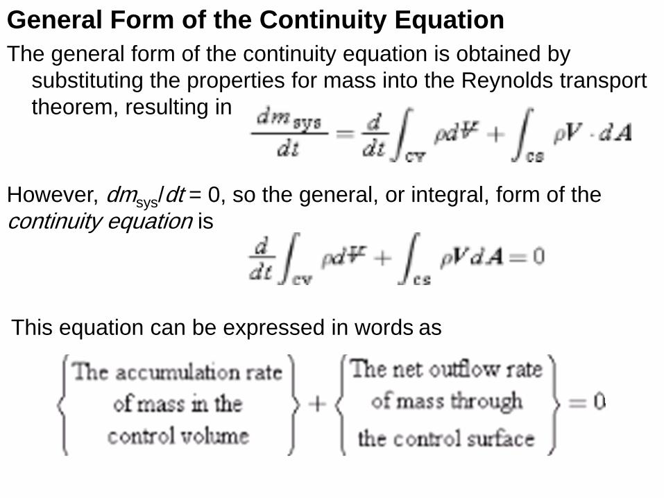
The general form of the continuity equation is obtained by

substituting the properties for mass into the Reynolds transport

theorem, resulting in

However, dmsys/dt = 0, so the general, or integral, form of the

continuity equation is

This equation can be expressed in words as

If the mass crosses the control surface through a number of inlet

and exit ports, the continuity equation simplifies to

where mcv is the mass of fluid in the control volume. Note that the

two summation terms represent the net mass outflow through the

control surface.

EXAMPLE 5.4 MASS ACCUMULATION IN A TANK

A jet of water discharges into an open tank, and water leaves the tank through an orifice in the bottom at a rate of 0.003 m3/s. If the cross-sectional area of the jet is 0.0025 m2 where the velocity of water is 7 m/s, at what rate is water accumulating in (or evacuating from) the tank

Solution 1. Continuity equation

Because there is only one

inlet and one outlet, the

equation reduces to

2. Term-by-term analysis

· The inlet mass flow rate is calculated as follows,

· Outlet flow rate is

3. Accumulation rate:

EXAMPLE 5.5 RATE OF WATER RISE IN

RESERVOIR

A river discharges into a reservoir at a rate of

11,3,00 m3/s, and the outflow rate from the

reservoir through the flow passages in the dam

is 7,000 m3/s. If the reservoir surface area is

100 km2, what is the rate of rise of water in the

reservoir?

Solution

Continuity equation:

Considering the control volume is constant, so dmcv/dt = 0

At the inlet, the mass flow rate is.

There two outlets in this case,

Substitution in the continuity equation,

The rate of rise simply is velocity,

smxxA

QQ

A

QV rise /103.4

10100

000,7300,11 5

6

1

21

1

=

=

==

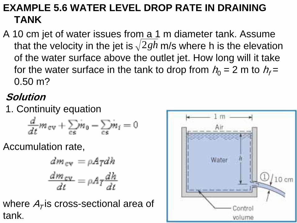
EXAMPLE 5.6 WATER LEVEL DROP RATE IN DRAINING

TANK

A 10 cm jet of water issues from a 1 m diameter tank. Assume

that the velocity in the jet is m/s where h is the elevation

of the water surface above the outlet jet. How long will it take

for the water surface in the tank to drop from h0 = 2 m to hf =

0.50 m?

gh2

Solution 1. Continuity equation

Accumulation rate,

where AT is cross-sectional area of

tank.

Inlet mass flow rate with no inflow is

The mass flow rate leaving is

Substitution of terms into continuity equation

Equation for elapsed time and separating variables

Integrating

Substituting in initial condition, h(0) = h0, and final condition, h(t) =

hf, and solving for time

Evaluating the parameters and calculating time

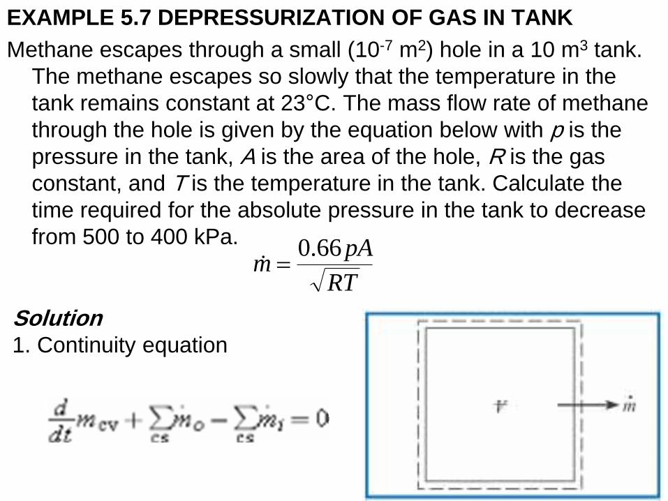
EXAMPLE 5.7 DEPRESSURIZATION OF GAS IN TANK

Methane escapes through a small (10-7 m2) hole in a 10 m3 tank.

The methane escapes so slowly that the temperature in the

tank remains constant at 23°C. The mass flow rate of methane

through the hole is given by the equation below with p is the

pressure in the tank, A is the area of the hole, R is the gas

constant, and T is the temperature in the tank. Calculate the

time required for the absolute pressure in the tank to decrease

from 500 to 400 kPa.

RT

pAm

66.0=

Solution 1. Continuity equation

Rate of accumulation term. The mass in the control volume is the sum of the mass of the tank shell, mshell and the mass of methane in the tank,

where V is the internal volume of the tank which is constant. The

mass of the tank shell is constant, so

= shellcv

mm

There is no mass inflow:

Mass out flow rate is

Substituting terms into continuity equation

Equation for elapsed time and Using ideal gas law for ρ,

Because R, T, A, and V are constant,

or

Integrating equation and substituting limits for initial and final

pressure and computing for time,

Continuity Equation for Flow in a Pipe

Several simplified forms of the continuity equation are used by engineers for flow in a pipe. Consider a control volume inside a pipe, Fig. 5.10. Mass enters through station 1 and exits through station 2. The control volume is fixed to the pipe walls, and its volume is constant. If the flow is steady, then mcv is constant so the mass flow formulation of the continuity equation reduces to

m1 = m2 fix

For flow with a uniform velocity and density distribution, the continuity equation for steady flow in a pipe is

If the flow is incompressible, then

or

Figure 5.10 Flow through a pipe section.

This equation is valid for

both steady and unsteady

incompressible flow.

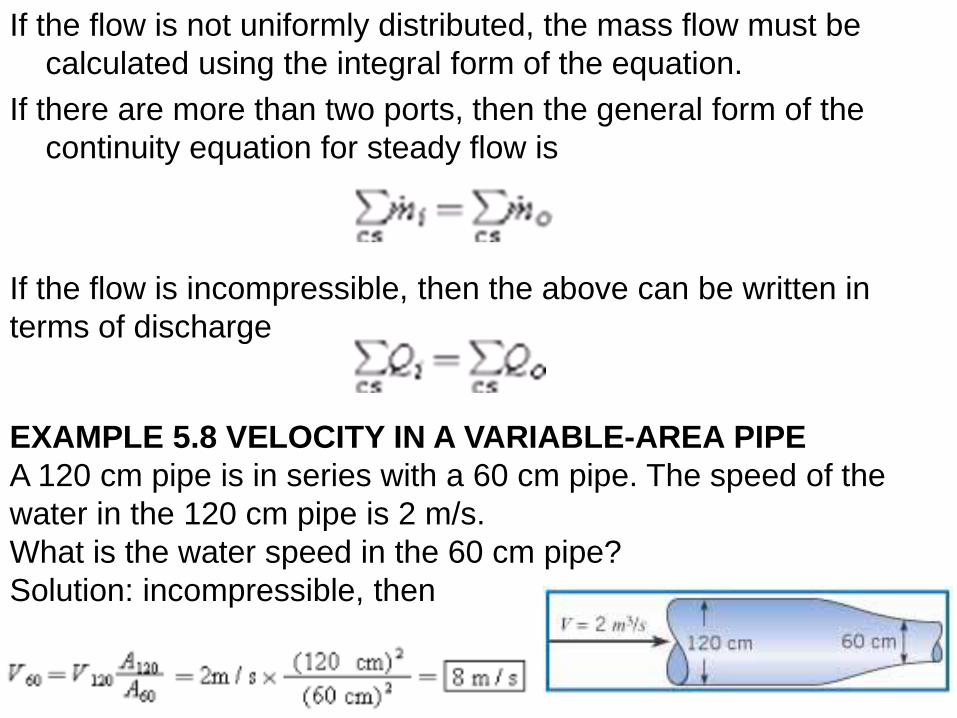
If the flow is not uniformly distributed, the mass flow must be

calculated using the integral form of the equation.

If there are more than two ports, then the general form of the

continuity equation for steady flow is

If the flow is incompressible, then the above can be written in

terms of discharge

EXAMPLE 5.8 VELOCITY IN A VARIABLE-AREA PIPE

A 120 cm pipe is in series with a 60 cm pipe. The speed of the

water in the 120 cm pipe is 2 m/s.

What is the water speed in the 60 cm pipe?

Solution: incompressible, then

EXAMPLE 5.9 WATER FLOW THROUGH A VENTURIMETER

Water with a density of 1000 kg/m3 flows through a vertical

venturimeter as shown. A pressure gage is connected across

two taps in the pipe (station 1) and the throat (station 2). The

area ratio Athroat/Apipe is 0.5. The velocity in the pipe is 10 m/s.

Find the pressure difference recorded by the pressure gage.

Assume the flow has a uniform velocity distribution and that

viscous effects are not important.

Solution:

The Bernoulli equation

Rewrite the equation in terms of

piezometric pressure.

Incompressible, then continuity equation V2/V1 = A1/A2

Gage is located at zero elevation. Apply hydrostatic equation

through static fluid in gage line between gage attachment point

where the pressure is and station 1 where the gage line is tapped

into the pipe,

But,

So,

5.4 Cavitation

Cavitation is the phenomenon that occurs when the fluid pressure is reduced to the local vapor pressure and boiling occurs. Under such conditions vapor bubbles form in the liquid, grow, and then collapse, producing shock waves, noise, and dynamic effects that lead to decreased equipment performance and, frequently, equipment failure. Engineers must design flow systems to avoid potential problems.

However, despite cavitation deleterious effects, cavitation can also be beneficial. Cavitation is responsible for the effectiveness of ultrasonic cleaning

Cavitation typically occurs at locations where the velocity is high. Consider the water flow through the pipe restriction shown in Fig. 5.11. The pipe area decreases, so the velocity increases according to the continuity equation and, in turn, the pressure decreases as dictated by the Bernoulli equation. For low flow rates, there is a relatively small drop in pressure at the restriction, so the water remains well above the vapor pressure and boiling does not occur. However, as the flow rate increases, the pressure at the restriction becomes progressively lower until a flow rate is reached where the pressure is equal to the vapor pressure. At this point, the liquid boils to form bubbles and cavitation ensues. The onset of cavitation can also be affected by the presence of contaminant gases, turbulence and viscosity.

Figure 5.11 Flow through pipe restriction: variation of pressure for three different flow rates.

The formation of vapor bubbles at the restriction is shown in Fig. 5.12a. The vapor bubbles form and then collapse as they move into a region of higher pressure and are swept downstream with the flow. When the flow velocity is increased further, the minimum pressure is still the local vapor pressure, but the zone of bubble formation is extended as shown in Fig. 5.12b. In this case, the entire vapor pocket may intermittently grow and collapse, producing serious vibration problems. Severe damage that occurred on a centrifugal pump impeller is shown in Fig. 5.13. Obviously, cavitation should be avoided or minimized by proper design of equipment and structures and by proper operational procedures.

Figure 5.12 Formation of vapor bubbles in the process of cavitation. (a) Cavitation. (b) Cavitation—higher flow rate.

Figure 5.13 Cavitation damage to impeller of a centrifugal pump.

5.5 Differential Form of the Continuity Equation

In the analysis of fluid flows and the development of numerical models, one of the fundamental independent equations needed is the differential form of the continuity equation. The derivation is accomplished by applying the integral form of the continuity equation to a small control volume and taking the limit as the volume approaches zero. A small control volume defined by the x, y, z coordinate system is shown in Fig. 5.15.

Figure 5.15 Elemental control volume.

When applying the integral form of the continuity to the differential

control volume one can eventually lead to

If the flow is steady, the equation reduces to

And if the fluid is incompressible, the equation further simplifies to

which is valid for both steady and unsteady flow. In vector

notation, Eq. (5.33) is given as

where is the del operator, defined as

Solution Continuity equation for two-dimensional flow:

EXAMPLE 5.10 APPLICATION OF DIFFERENTIAL FORM OF

COBTINUITY EQUATION

The expression V = 10xi - 10yj is said to represent the velocity for

a two-dimensional (planar) incompressible flow. Check to see if

the continuity equation is satisfied.