FLUENT - Compressible Flow in a Nozzle- Problem Specification

Problem Specification

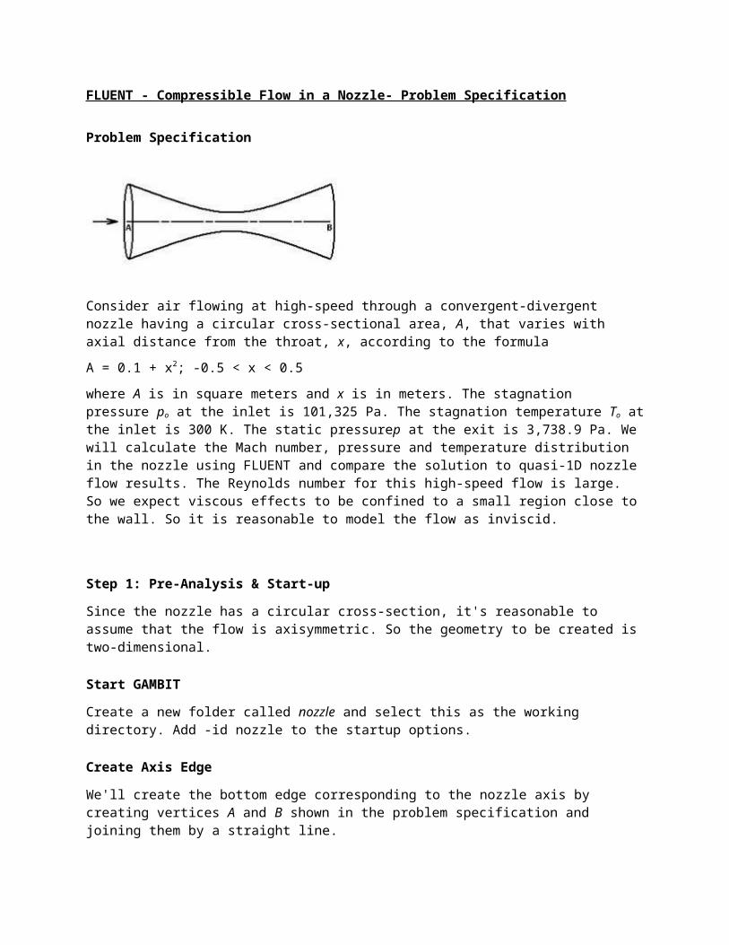
Consider air flowing at high-speed through a convergent-divergent nozzle having a circular cross-sectional area, A, that varies with axial distance from the throat, x, according to the formula

A = 0.1 + x2; -0.5 < x < 0.5

where A is in square meters and x is in meters. The stagnation pressure po at the inlet is 101,325 Pa. The stagnation temperature To at the inlet is 300 K. The static pressurep at the exit is 3,738.9 Pa. We will calculate the Mach number, pressure and temperature distribution in the nozzle using FLUENT and compare the solution to quasi-1D nozzle flow results. The Reynolds number for this high-speed flow is large. So we expect viscous effects to be confined to a small region close to the wall. So it is reasonable to model the flow as inviscid.

Step 1: Pre-Analysis & Start-up

Since the nozzle has a circular cross-section, it's reasonable to assume that the flow is axisymmetric. So the geometry to be created is two-dimensional.

Start GAMBIT

Create a new folder called nozzle and select this as the working directory. Add -id nozzle to the startup options.

Create Axis Edge

We'll create the bottom edge corresponding to the nozzle axis by creating vertices A and B shown in the problem specification and joining them by a straight line.

Operation Toolpad > Geometry Command Button   >Vertex Command Button   

>Create Vertex 

Create the following two vertices:

Vertex 1: (-0.5,0,0)Vertex 2: (0.5,0,0)

Operation Toolpad > Geometry Command Button   > Edge Command Button   > Create Edge 

Select vertex 1 by holding down the Shift button and clicking on it. Next, select vertex 2. Click Apply in the Create Straight Edge window.

Create Wall Edge

We'll next create the bottom edge corresponding to the nozzle wall. This edge is curved. Since

A = Πr2

where r( x ) is the radius of the cross-section at x and

A = 0.1 + x2

for the given nozzle geometry, we get

r( x ) = [(0.1 + x2)/Π]0.5; -0.5 < x < 0.5

This is the equation of the curved wall. Life would have been easier if GAMBIT allowed for this equation to be entered directly to create the curved edge. Instead, one has to create a file containing the coordinates of a series of points along the curved line and read in the file. The more number of points used along the curved edge, the smoother the resultant edge.

The file vert.dat contains the point definitions for the nozzle wall. Take a look at this file. The first line is

21 1

which says that there are 21 points along the edge and we are defining only 1 edge. This is followed by x,r and z coordinates for each point along the edge. The r-value for each x was generated from the above equation for r( x ) . The z-coordinate is 0 for all points since we have a 2D geometry.

Right-click on vert.dat and select Save As... to download the file to your working directory.

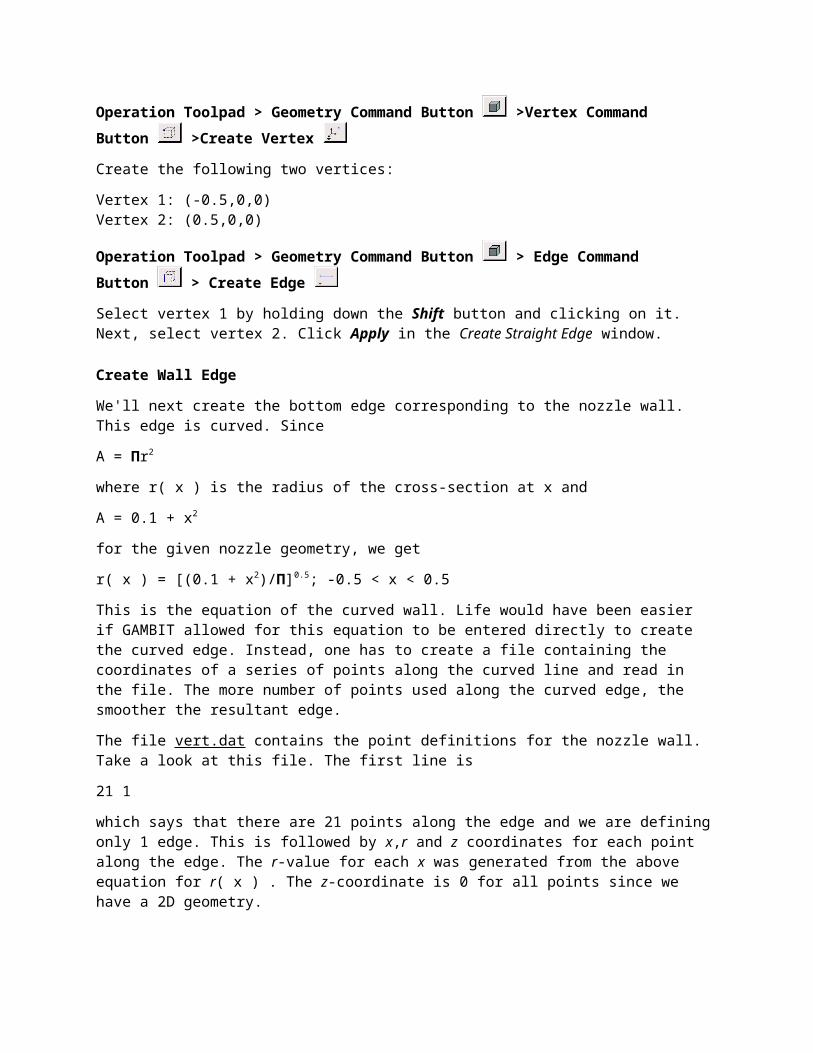
Main Menu > File > Import > ICEM Input ...

Next to File Name:, enter the path to the vert.dat file that you downloaded or browse to it by clicking on the Browse button.

Then, check the Vertices and Edges boxes under Geometry to Create as we want to create the vertices as well as the curved edge.

Click Accept.

This should create the curved edge. Here it is in relation to the vertices we created above:

Higher Resolution Image

Create Inlet and Outlet Edges

Create the vertical edge for the inlet:

Operation Toolpad > Geometry Command Button   > Edge Command Button  > Create Edge

Shift-click on vertex 1 and then the vertex above it to create the inlet edge.

Similarly, create the vertical edge for the outlet.

Higher Resolution Image

Create Face

Form a face out of the area enclosed by the four edges:

Operation Toolpad > Geometry Command Button   >Face Command Button   >Form Face 

Recall that we have to shift-click on each of the edges enclosing the face and then click Apply to create the face.

Save Your Work

Main Menu > File > Save

This will create the nozzle.dbs file in your working directory. Check that it has been created so that you will able to resume from here if necessary.

Step 2: Geometry

Now that we have the basic geometry of the nozzle created, we need to mesh it. We would like to create a 50x20 grid for this geometry.

Mesh Edges

As in the previous tutorials, we will first start by meshing the edges.

Operation Toolpad > Mesh Command Button    > Edge Command Button   > Mesh Edges 

Like the Laminar Pipe Flow Tutorial, we are going to use even spacing between each of the mesh points. We won't be using the Grading this time, so deselect the box next to Grading that says Apply.

Then, change Interval Count to 20 for the side edges and Interval Count to 50 for the top and bottom edges.

Higher Resolution Image

Mesh Face

Now that we have the edges meshed, we need to mesh the face.

Operation Toolpad > Mesh Command Button    > Face Command Button    > Mesh Faces  As before, select the face and click the Apply button.

Higher Resolution Image

Save Your Work

Main Menu > File > Save

Step 3: Mesh

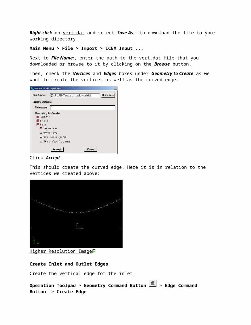
Specify Boundary Types

Now that we have the mesh, we would like to specify the boundary conditions here in GAMBIT.

Operation Toolpad > Zones Command Button    > Specify Boundary Types Command Button 

This will bring up the Specify Boundary Types window on the Operation Panel. We will first specify that the left edge is the inlet. Under Entity:, pick Edges so that GAMBITknows we want to pick an edge (face is default).

Now select the left edge by Shift-clicking on it. The selected edge should appear in the yellow box next to the Edges box you just worked with as well as the Label/Typelist right under the Edges box.

Next to Name:, enter inlet.

For Type:, select WALL.

Click Apply. You should see the new entry appear under Name/Type box near the top of the window.

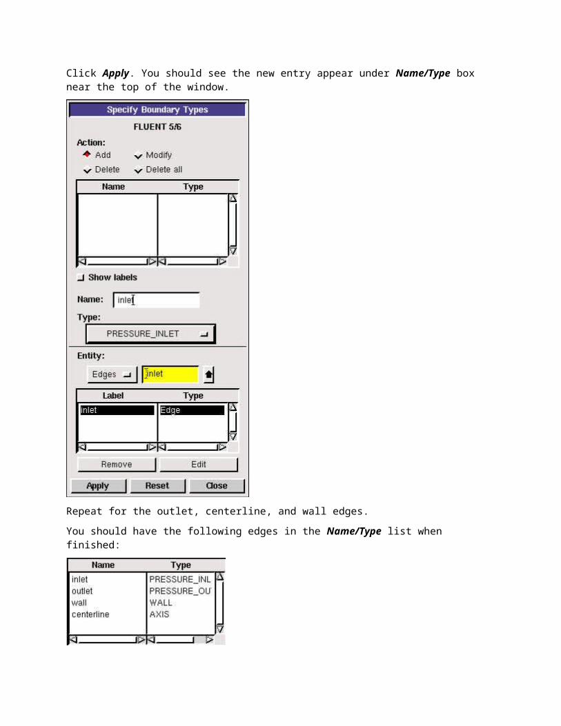
Repeat for the outlet, centerline, and wall edges.

You should have the following edges in the Name/Type list when finished:

Save and Export

Main Menu > File > Save

Main Menu > File > Export > Mesh...

Type in nozzle.msh for the File Name:. Select Export 2d Mesh since this is a 2 dimensional mesh. Click Accept.

Check nozzle.msh has been created in your working directory.

Step 4: Setup (Physics)

Useful InformationIconThese instructions are for FLUENT 6.3.26. Click here for instructions for FLUENT 12.

If you have skipped the previous mesh generation steps 1-3, you can download the mesh by right-clicking on this link. Save the file as nozzle.msh in your working directory. You can then proceed with the flow solution steps below. 

Launch FLUENT

Start > Programs > Fluent Inc > FLUENT 6.3.26 > FLUENT 6.3.26

Select 2ddp from the list of options and click Run.

Import File

Main Menu > File > Read > Case...

Navigate to your working directory and select the nozzle.msh file. Click OK.

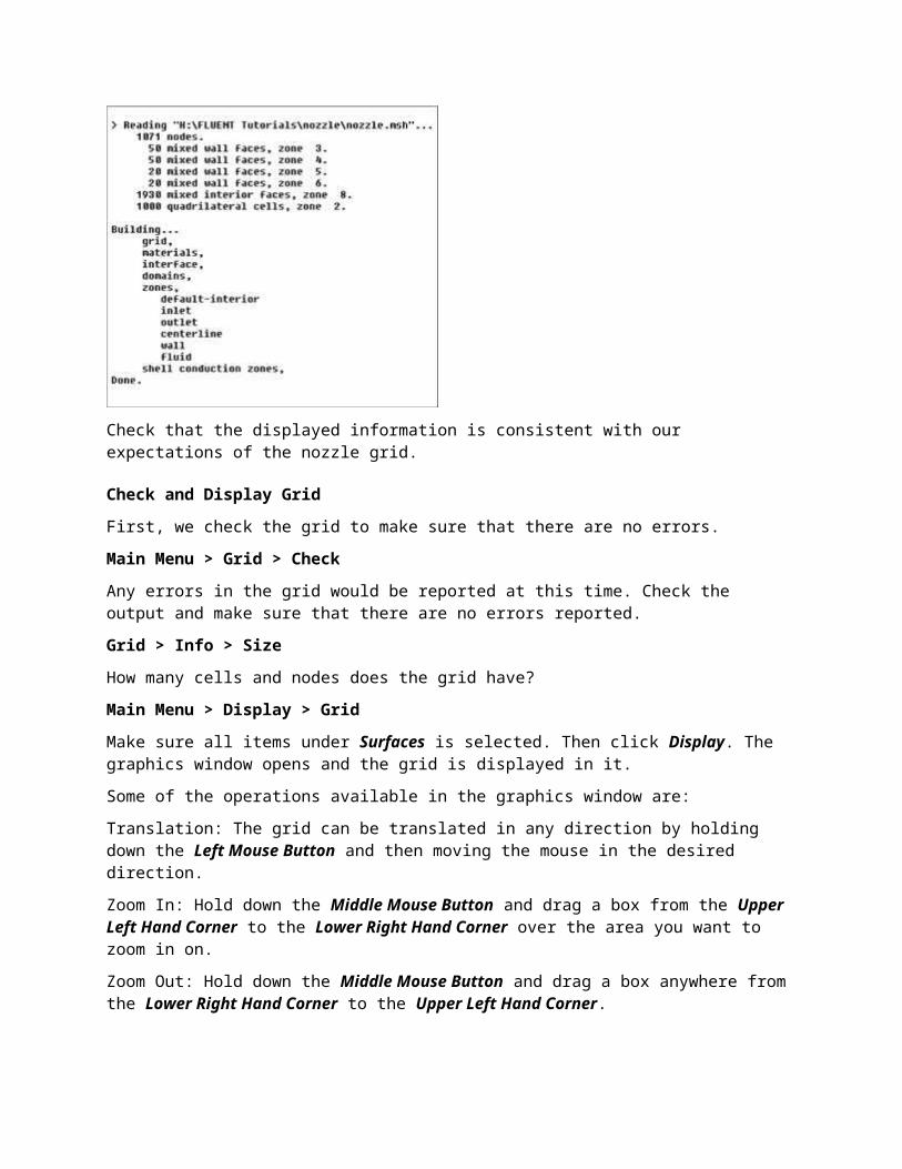
The following should appear in the FLUENT window:

Check that the displayed information is consistent with our expectations of the nozzle grid.

Check and Display Grid

First, we check the grid to make sure that there are no errors.

Main Menu > Grid > Check

Any errors in the grid would be reported at this time. Check the output and make sure that there are no errors reported.

Grid > Info > Size

How many cells and nodes does the grid have?

Main Menu > Display > Grid

Make sure all items under Surfaces is selected. Then click Display. The graphics window opens and the grid is displayed in it.

Some of the operations available in the graphics window are:

Translation: The grid can be translated in any direction by holding down the Left Mouse Button and then moving the mouse in the desired direction.

Zoom In: Hold down the Middle Mouse Button and drag a box from the Upper Left Hand Corner to the Lower Right Hand Corner over the area you want to zoom in on.

Zoom Out: Hold down the Middle Mouse Button and drag a box anywhere from the Lower Right Hand Corner to the Upper Left Hand Corner.

The grid has 50 divisions in the axial direction and 20 divisions in the radial direction. The total number of cells is 50x20=1000. Since we are assuming inviscid flow, we won't be resolving the viscous boundary layer adjacent to the wall. (The effect of the boundary layer is small in our case and can be neglected.) Thus, we don't need to cluster nodes towards the wall. So the grid has uniform spacing in the radial direction. We also use uniform spacing in the axial direction.

Look at specific parts of the grid by choosing each boundary (centerline, inlet, etc) listed under Surfaces in the Grid Display menu. Click to select and click again to deselect a specific boundary. Click Display after you have selected your boundaries.

Define Solver Properties

Define > Models > Solver...

We see that FLUENT offers two methods ("solvers") for solving the governing equations: Pressure-Based and Density-Based. To figure out the basic difference between these two solvers, let's turn to the documentation.

Main Menu > Help > User's Guide Contents ...

This should bring up FLUENT 6.3 User's Guide in your web browser. If not, access the User's Guide from the Start menu: Start > Programs > Fluent Inc Products > Fluent 6.3 Documentation > Fluent 6.3 Documentation. This will bring up the FLUENT documentation in your browser. Click on the link to the user's guide.

Go to chapter 25 in the user's guide; it discusses the Pressure-Based and Density-Based solvers. Section 25.1 introduces the two solvers:

"Historically speaking, the pressure-based approach was developed for low-speed incompressible flows, while the density-based approach was mainly used for high-speed compressible flows. However, recently both methods have been extended and reformulated to solve and operate for a wide range of flow conditions beyond their traditional or original intent."

"In both methods the velocity field is obtained from the momentum equations. In the density-based approach, the continuity equation is used to obtain the density field while the pressure field is determined from the equation of state."

"On the other hand, in the pressure-based approach, the pressure field is extracted by solving a pressure or pressure correction equation which is obtained by manipulating continuity and momentum equations."

Mull over this and the rest of this section. So which solver do we use for our nozzle problem? Turn to section 25.7.1 in chapter 25:

"The pressure-based solver traditionally has been used for incompressible and mildly compressible flows. The density-based approach, on the other hand, was originally designed for high-speed compressible flows. Both approaches are now applicable to a broad range of flows (from incompressible to highly compressible), but the origins of the density-based formulation may give it an accuracy (i.e. shock resolution) advantage over the pressure-based solver for high-speed compressible flows."

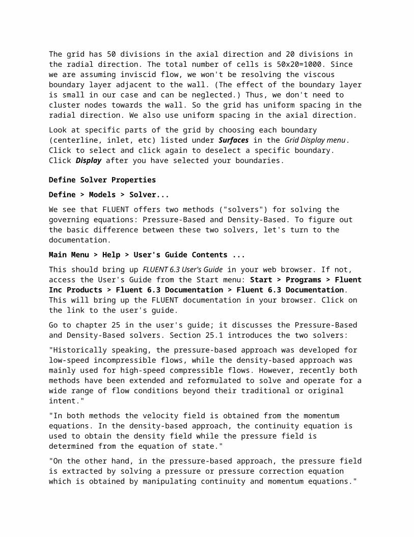
Since we are solving a high-speed compressible flow, let's pick the density-based solver.

In the Solver menu, select Density Based.

Under Space, choose Axisymmetric. This will solve the axisymmetric form of the governing equations.

Click OK.

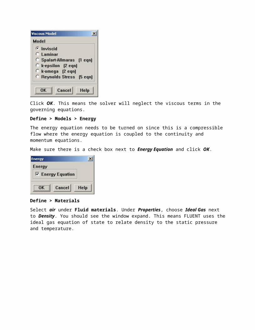
Define > Models > Viscous

Select Inviscid under Model.

Click OK. This means the solver will neglect the viscous terms in the governing equations.

Define > Models > Energy

The energy equation needs to be turned on since this is a compressible flow where the energy equation is coupled to the continuity and momentum equations.

Make sure there is a check box next to Energy Equation and click OK.

Define > Materials

Select air under Fluid materials. Under Properties, choose Ideal Gas next to Density. You should see the window expand. This means FLUENT uses the ideal gas equation of state to relate density to the static pressure and temperature.

Click Change/Create. Close the window.

Define > Operating Conditions

We'll work in terms of absolute rather than gauge pressures in this example. So set Operating Pressure in the Pressure box to 0.

Click OK.

It is important that you set the operating pressure correctly in compressible flow calculations since FLUENT uses it to compute absolute pressure to use in the ideal gas law.

Define > Boundary Conditions

Set boundary conditions for the following surfaces: inlet, outlet, centerline, wall.

Select inlet under Zone and pick pressure-inlet under Type as its boundary condition. Click Set.... The Pressure Inlet window should come up.

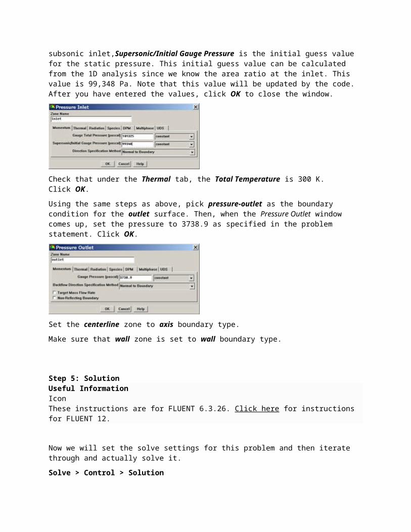
Set the total pressure (noted as Gauge Total Pressure in FLUENT) at the inlet to 101,325 Pa as specified in the problem statement. For a subsonic inlet,Supersonic/Initial Gauge Pressure is the initial guess value for the static pressure. This initial guess value can be calculated from the 1D analysis since we know the area ratio at the inlet. This value is 99,348 Pa. Note that this value will be updated by the code. After you have entered the values, click OK to close the window.

Check that under the Thermal tab, the Total Temperature is 300 K. Click OK.

Using the same steps as above, pick pressure-outlet as the boundary condition for the outlet surface. Then, when the Pressure Outlet window comes up, set the pressure to 3738.9 as specified in the problem statement. Click OK.

Set the centerline zone to axis boundary type.

Make sure that wall zone is set to wall boundary type.

Step 5: SolutionUseful InformationIconThese instructions are for FLUENT 6.3.26. Click here for instructions for FLUENT 12.

Now we will set the solve settings for this problem and then iterate through and actually solve it.

Solve > Control > Solution

We'll just use the defaults. Note that a second-order discretization scheme will be used. Click OK.

Set Initial Guess

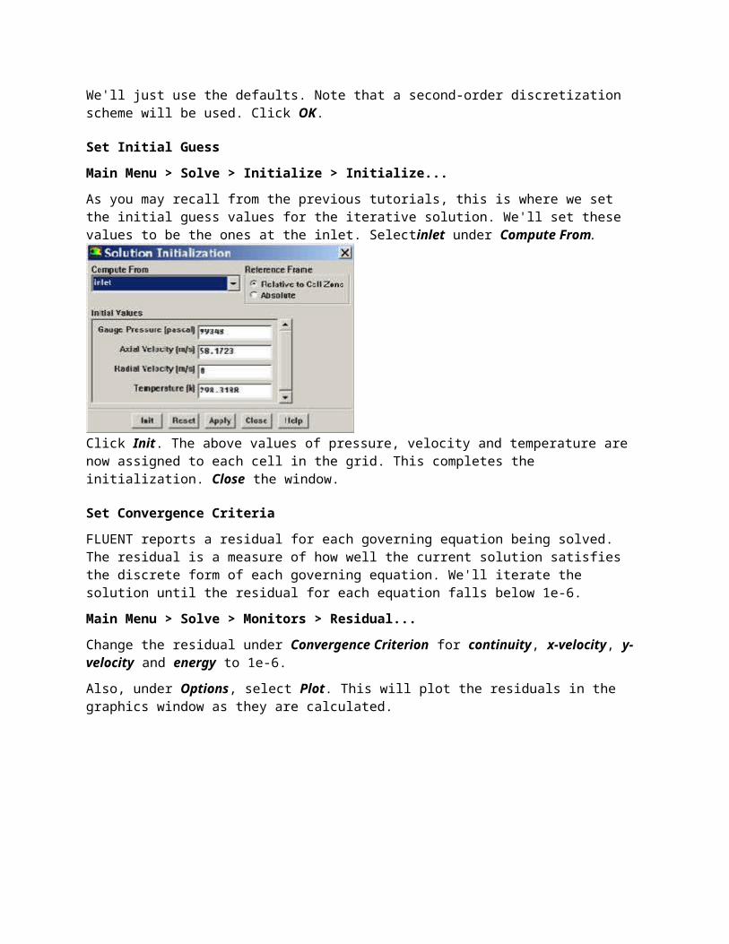
Main Menu > Solve > Initialize > Initialize...

As you may recall from the previous tutorials, this is where we set the initial guess values for the iterative solution. We'll set these values to be the ones at the inlet. Selectinlet under Compute From.

Click Init. The above values of pressure, velocity and temperature are now assigned to each cell in the grid. This completes the initialization. Close the window.

Set Convergence Criteria

FLUENT reports a residual for each governing equation being solved. The residual is a measure of how well the current solution satisfies the discrete form of each governing equation. We'll iterate the solution until the residual for each equation falls below 1e-6.

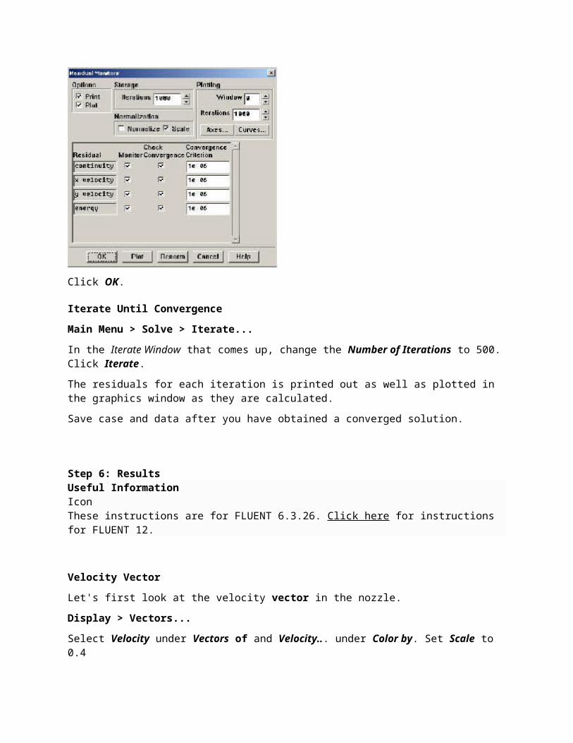
Main Menu > Solve > Monitors > Residual...

Change the residual under Convergence Criterion for continuity, x-velocity, y-velocity and energy to 1e-6.

Also, under Options, select Plot. This will plot the residuals in the graphics window as they are calculated.

Click OK.

Iterate Until Convergence

Main Menu > Solve > Iterate...

In the Iterate Window that comes up, change the Number of Iterations to 500. Click Iterate.

The residuals for each iteration is printed out as well as plotted in the graphics window as they are calculated.

Save case and data after you have obtained a converged solution.

Step 6: ResultsUseful InformationIconThese instructions are for FLUENT 6.3.26. Click here for instructions for FLUENT 12.

Velocity Vector

Let's first look at the velocity vector in the nozzle.

Display > Vectors...

Select Velocity under Vectors of and Velocity... under Color by. Set Scale to 0.4

 Click Display. 

Higher Resolution Image

We see that the flow is smoothly accelerating from subsonic to supersonic.To include the lower half of nozzle, do the following:Icon Display > Views...Select centerline and click ApplyWhite Background on Graphics Window

IconTo get white background go to:Main Menu > File > HardcopyMake sure that Reverse Foreground/Background is checked and select Color in Coloring section. Click Preview. Click No when prompted "Reset graphics window?"

Mach Number Contour

Let's now look at the Mach number

Display > Contours

Select Velocity... under Contours of and select Mach Number. Set Levels to 30. 

 Click Display. 

Higher Resolution Image

  

For 1D case, mach number is a function of x position. For 1D case, we are supposed to see vertical contour of mach numbers that are parallel to each other. 

For 2D case, we are seeing curving contour of mach number. The deviation from vertical indicates the 2D effect. 

Do note that 1D approximation is fairly accurate around the centerline of nozzle.

Pressure Contour Plot

Let's look at how pressure changes in the nozzle.

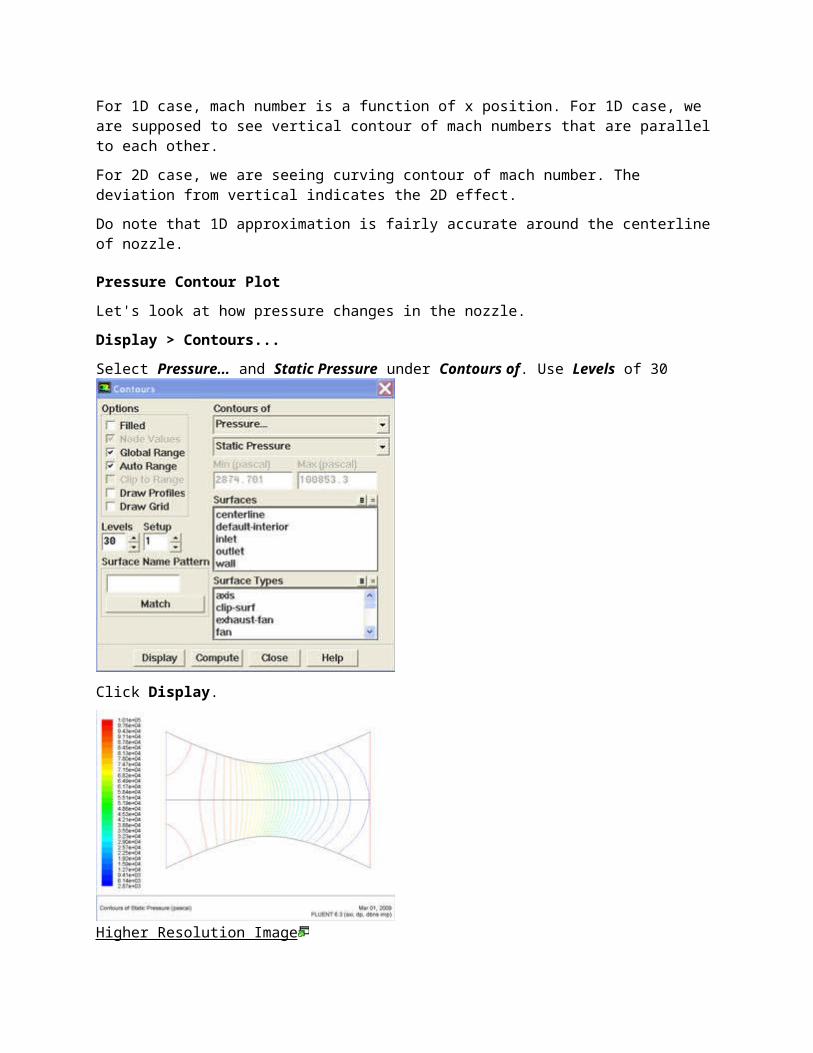
Display > Contours...

Select Pressure... and Static Pressure under Contours of. Use Levels of 30 

Click Display. 

Higher Resolution Image

  

Notice that the pressure decreases as it flows to the right. 

Total Pressure Contour Plot

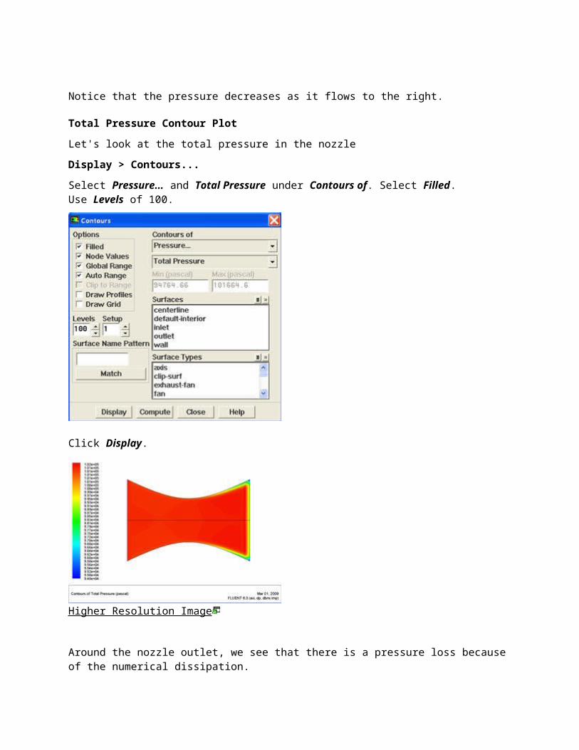
Let's look at the total pressure in the nozzle

Display > Contours...

Select Pressure... and Total Pressure under Contours of. Select Filled. Use Levels of 100.

 Click Display.

Higher Resolution Image

  

Around the nozzle outlet, we see that there is a pressure loss because of the numerical dissipation. 

Temperature Contour Plot

Let's investigate or verify the temperature properties in the nozzle.

Display > Contours...

Select Temperature... and Static Temperature under Contours of. Use Levels of 30.

 Click Display. 

Higher Resolution Image

  

As we can see, the temperature decreases from left to right in the nozzle, indicating a transfer of internal energy to kinetic energy as the fluid speeds up. 

Total Temperature Contour Plot

Let's look at the total pressure in the nozzle

Display > Contours...

Select Temperature... and Total Temperature under Contours of. Select Filled. Use Levels of 100.

 Click Display. 

Higher Resolution Image

  

Looking at the scale, we see that the total temperature is uniform 300 K throughout the nozzle. The contour abnormality at the outlet of the nozzle is due to the round off errors. 

Pressure Plot

Let's look at the pressure along the centerline and the wall. 

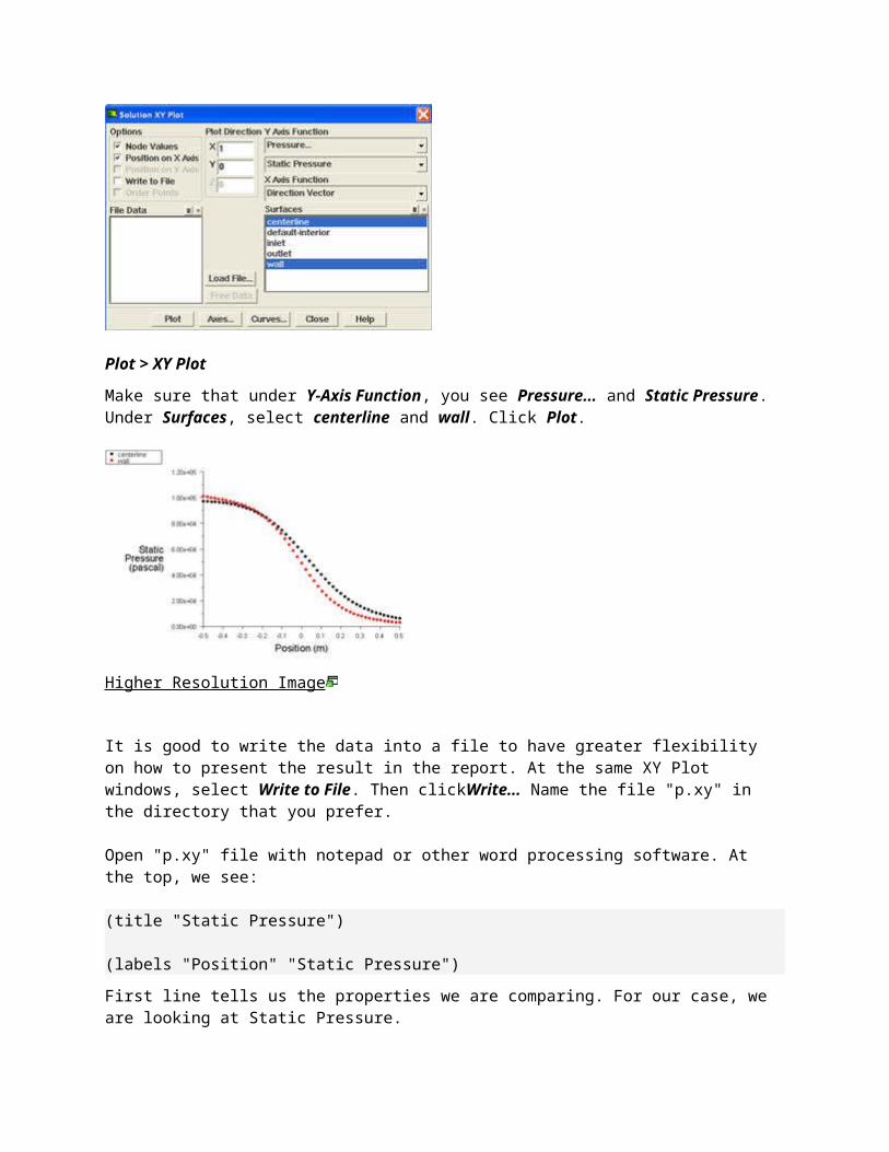
 Plot > XY Plot

Make sure that under Y-Axis Function, you see Pressure... and Static Pressure. Under Surfaces, select centerline and wall. Click Plot. 

Higher Resolution Image

  

It is good to write the data into a file to have greater flexibility on how to present the result in the report. At the same XY Plot windows, select Write to File. Then clickWrite... Name the file "p.xy" in the directory that you prefer. Open "p.xy" file with notepad or other word processing software. At the top, we see: (title "Static Pressure")

(labels "Position" "Static Pressure")

First line tells us the properties we are comparing. For our case, we are looking at Static Pressure.Second line tells us about the x and y label. There is a header at the beginning of each the data sets so that we can differentiate which data sets we are looking at. For our case, we have "centerline" and "wall" data sets.

 Following is an example of two data sets (centerline and wall).

((xy/key/label "centerline")

-0.5    97015.3

-0.48    96949.9

.

.

.

0.5    6012.92

)

((xy/key/label "wall")

-0.5    100853

-0.480911    100496

.

.

.

0.5    2874.7

)

Try copy the appropriate data sets to excel and plot the results.

  

Mach Number Plot

Let's plot the variation of Mach number in the axial direction at the axis and wall. In addition, we will plot the corresponding variation from 1D theory. You can download the file here: mach_1D.xy.Plot > XY PlotUnder the Y Axis Function, select Velocity... and Mach Number.

Also, since we are going to plot this number at both the wall and axis, select centerline and wall under Surfaces.

Then, load the mach_1D.xy by clicking on Load File....

Click Plot. 

Higher Resolution Image

  

How does the FLUENT solution compare with the 1D solution?

Is the comparison better at the wall or at the axis? Can you explain this?

Save this plot as machplot.xy by checking Write to File and clicking Write.... 

Step 7: Verification & Validation

Solve the nozzle flow for the same conditions as used in class on a 80x30 grid. Recall that the static pressure p at the exit is 3,738.9 Pa. The grid for this calculation can be downloaded here.

(a) Plot the variation of Mach number at the axis and the wall as a function of the axial distance x. Also, plot the corresponding results obtained on the 50x20 grid used in class and from the quasi-1D assumption. Recall that the quasi-1D result for the Mach number variation was given to you in the M_1D.xy file. Note all five curves should be plotted on the same graph so that you can compare them. You can make the plots in FLUENT, MATLAB or EXCEL.

(b) Plot the variation of static pressure at the axis and the wall as a function of the axial distance x. Also, plot the corresponding results obtained on the 50x20 grid used in class and from the quasi-1D assumption. Calculate the static pressure variation for the quasi-1D case from the Mach number variation given in M_1D.xy.

(c) Plot the variation of static temperature at the axis and the wall as a function of the axial distance x. Also, plot the corresponding results obtained on the 50x20 grid used in class and from the quasi-1D assumption. Calculate the static temperature variation for the quasi-1D case from the Mach number variation given in M_1D.xy.

Comment very briefly on the grid dependence of your results and the comparison with the quasi-1D results.

Problem 1

Consider the nozzle flow problem solved using FLUENT in the tutorial. Recall that the nozzle has a circular cross-sectional area, A, that varies with axial distance from the throat, x, according to the formula:

A = 0.1 + x2

where A is in square meters and x is in meters. The stagnation pressure poand stagnation temperature To at the inlet are 101,325 Pa and 300 K, respectively.

Using the quasi-1D flow assumption, determine the static pressure at the nozzle inlet and outlet for the following conditions:

(a) Sonic flow at the throat, and supersonic, isentropic flow in the diverging section.(b) Sonic flow at the throat, and subsonic, isentropic flow in the diverging section.(c) Sonic flow at the throat and normal shock at the exit.

Problem 2

Change the exit pressure to 40,000 Pa while keeping all the other boundary conditions the same. What flow regime do you expect for this exit pressure based on the quasi-1D results in problem 1? Re-run the FLUENT calculation with this exit pressure on the 50x20 grid.

(a) Plot contours of the Mach number and static pressure for this case. Is the flow regime as predicted by quasi-1D theory? Explain briefly the possible causes for any similarities or disparities.

(b) Plot the static and stagnation pressures at the axis as a function of the axial distance. Also, plot the corresponding values from the case where the exit pressure is 3,738.9 Pa. (These four curves should be on the same graph.) Explain briefly the salient features of this plot.

(c) Plot the static and stagnation temperatures at the axis as a function of the axial distance. Again provide a brief explanation for the salient features.