Five crisp and fuzzy models for supply chain of an ... crisp and fuzzy models for supply chain of an...

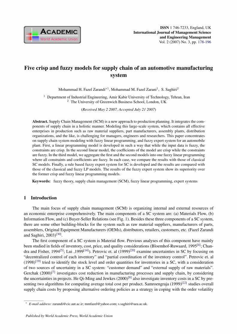
ISSN 1 746-7233, England, UKInternational Journal of Management Science

and Engineering ManagementVol. 2 (2007) No. 3, pp. 178-196

Five crisp and fuzzy models for supply chain of an automotive manufacturingsystem

Mohammad H. Fazel Zarandi∗1, Mohammad M. Fazel Zarani1, S. Saghiri2

1 Department of Industrial Engineering, Amir Kabir University of Technology, Tehran, Iran2 The University of Greenwich Business School, London, UK

(Received May 2 2007, Accepted July 21 2007)

Abstract. Supply Chain Management (SCM) is a new approach to production planning. It integrates the com-ponents of supply chain in a holistic manner. Modeling this large-scale system, which contains all effectiveenterprises in production such as raw material suppliers, part manufacturers, assembly plants, distributionorganizations, and the like, is challenging for managers, engineers and researchers. This paper concentrateson supply chain system modeling with fuzzy linear programming, and fuzzy expert system for an automobileplant. First, a linear programming model is developed in such a way that while the input data is fuzzy, theconstraints are crisp. In the second linear model, the coefficients of the model are crisp while the constraintsare fuzzy. In the third model, we aggregate the first and the second models into one fuzzy linear programmingwhere all constraints and coefficients are fuzzy. In each case, we compare the results with those of classicalSC models. Finally, a rule based fuzzy expert system for SC is developed and the results are compared withthose of the classical and fuzzy LP models. The results of the fuzzy expert system show its superiority overthe former crisp and fuzzy linear programming models.

Keywords: fuzzy theory, supply chain management (SCM), fuzzy linear programming, expert systems

1 Introduction

The main focus of supply chain management (SCM) is organizing internal and external resources ofan economic enterprise comprehensively. The main components of a SC system are: (a) Materials Flow, (b)Information Flow, and (c) Buyer-Seller Relations (see Fig. 1). Besides these three components of a SC system,there are some other building-blocks for the system such as raw material suppliers, manufacturers of parts,assemblers, Original Equipment Manufacturers (OEMs), distributors, retailers, customers, etc. (Fazel Zarandiand Saghiri, 2003)[30].

The first component of a SC system is Material flow. Previous analyses of this component have mainlybeen studied in fields of inventory, cost, price, and quality considerations (Bloemhof-Ruwaard, 1995[4]; Chan-dra and Fisher, 1994[5]; Lui ,1999[14]). Petrovic et. al (1999)[20] examine uncertainties in SC by focusing on“decentralized control of each inventory” and “partial coordination of the inventory control”. Petrovic et. al(1998)[19] tried to identify the stock level and order quantities for inventories in a SC, with a considerationof two sources of uncertainty in a SC system: “customer demand” and “external supply of raw materials”.Gerchak (2000)[7] investigates cost reduction in manufacturing processes and supply chain, by consideringthe uncertainties in projects. He Qi-Ming and Jewkes (2000)[8] also investigate inventory costs in a SC by pre-senting two algorithms for computing average total cost per product. Samroengraja (1999)[22] studies overallsupply chain costs by proposing alternative ordering policies as a strategy in coping with the order volatility

∗ E-mail address: [email protected]; [email protected]; [email protected].

Published by World Academic Press, World Academic Union

International Journal of Management Science and Engineering Management, Vol. 2 (2007) No. 3, pp. 178-196 179

in a SC. Cost analysis, storage and warehousing, and quality management systems are some other interestingareas in SC (Mullins, 1999[17]; Elinger, 2000[1]).

Fig. 1. Material Flow, Information Flow, and Buyer-Seller Relations in a supply chain system (Fazel Zarandi et al.,2002)[32]

The second component of a SC is information flow. Companies’ Information Technology (IT) strategiesin their SC, role of the IT in cost reduction of SCM, and IT-SC inter-relationships are some of the main aspectsof information flow in SC (Lancioni, 2000[12]; Lancioni and Smith, 2000[13])

The third component of a SC system is Buyer-Seller Relations. Monczka et al. (1998)[16] investigatesuccess factors in strategic supplier alliances. Stuart (1993)[24] surveys influencing factors in supplier partner-ships as well as potential and strategic benefits of such a policy. Ohmae (1989)[18] has defined a global logic ofstrategic partnerships and alliances aspects: “World competition”, “need to market expansion and finding ordeveloping new market” and some other related topics in Business Planning Process. Heide and John (1990)[9]

pursue alliances in industrial purchasing that lead supply chains to more unification and harmonized operation.As a matter of fact, in a way to achieving maximum efficiency in performance of its components, SC

could be modeled as a large and complex system. However, modeling real world SC systems are very difficult.The main problems with classical SC models are high complexity, lack of flexibility and uncertainty embeddedin them.

The hypothesis in this paper is that fuzzy system modeling and approximate reasoning are suitable toolsto represent three main aspects of real systems: complexity, flexibility, and reliability. Our approach for thedevelopment of SC models in this paper is to investigate a gradual transition from a totally crisp LP model toa completely fuzzy one and next to a linguistic fuzzy expert system model to see if the behavior of the systemcan better be represented.

The rest of the paper is organized as follows: first, uncertainties in SC systems will be investigated and abrief review of fuzzy logic and fuzzy set theory will be presented. Then, a case study of a SC system will bedemonstrated for an automobile industry. Models for such a system are developed through classical and fuzzyoperation research (OR) models in three steps: (i) a linear programming (LP) model with fuzzy coefficients,(ii) an LP model with fuzzy bounds and objective function, and (iii) an LP model with fuzzy coefficients,fuzzy bounds and objective function. Finally, the same case study will be modeled and analyzed via fuzzyexpert system (FES) approach. The results of all four approaches are compared and their advantages anddisadvantages are articulated.

MSEM email for subscription: [email protected]

180 M. Zarandi & M. Zarani & S. Saghiri: Five crisp and fuzzy models

2 Fuzzy concepts for SCM

Real world production management, planning, and control problems are usually imprecise, complex,and critically depend on human activities. However managers are to interact in an intelligent way with thisenvironment. Thus, they have to reach out for new kind of reasoning based on such situation. (Turksen andFazel Zarandi, 1999)[27]. A SC system usually contains several sub-systems with unlimited relations andinterfaces. Each subsystem and its interfaces with others in the context of Material Flow, Information Flow,and Suppler-Buyer relations naturally contain a lot of uncertainties. It is a challenge to model a SC with anintegrated approach and to capture relations between different elements of such a chain (Chen and Tzeng2000)[6]. Petrovic et al. (1999)[20] demonstrate the uncertainties in SC systems as follows:

“· · · A real SC operates in an uncertain environment. Different sources and types of uncertainty existalong the SC. There are possible events, uncertainties in judgment, some lack of evidence, as well as a lack ofcertainty in available evidence. They appear in customer demand, production processes and supply sources.Each facility in the SC must deal with uncertain demand imposed by succeeding facilities and uncertaindelivery of the preceding facilities in the SC · · · ” (Petrovic et al., 1999)[20].

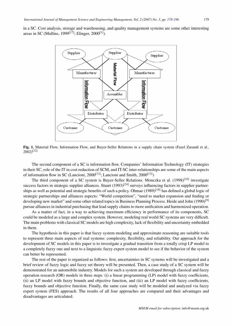
On the other hand, influencing several factors on the performance of a SC system as well as its depen-dence on human activities, make it naturally complex. In a SC system design and modeling, we have to dealwith a large-scale socio-technical system where classical quantitative approaches do not provide satisfactoryanswers–see Fig. 2 (Sugeno and Yasukawa, 1993[26]; Turksen, 1992[28]).

Fig. 2. Relation between SC system fuzziness and flow of material and information in it

Concerning above characteristics of SC system, applying fuzzy concepts and theory seems appropriatein SCM. In mathematical foundations of the fuzzy theory, there exists enough flexibility subject to certainaxioms. In fuzzy systems, it is not difficult to merge hard and soft constraints. Moreover, the main source ofdifficulty for constructing reasonable production planning and scheduling stems from conflicting nature of thecriteria and goals. Fuzzy approach provides tools to satisfy constraints to certain degree and to take into ac-count the relative importance in a format easily understood by human experts (Turksen, 1992[28]; Zimmerman,1996[33]).

Our hypothesis is that SC is a complex system with imprecise parameters and conditions and it canbe analyzed and modeled by using fuzzy set theory, more appropriately. In sum, the fuzzy systems approachdemonstrates many advantages in real world applications like SC systems that could be summarized as follows(Turksen and Fazel Zarandi, 1999)[27].

(1) Fuzzy systems are conceptually easy to understand.(2) Fuzzy systems are flexible, and with any given system, it is easy to mange it or layer more function-

ality on top of it without staring again from scratch.(3) Fuzzy systems can model most nonlinear functions of arbitrary complexity.(4) Fuzzy systems are tolerant of imprecise data.

MSEM email for contribution: [email protected]


(5) Fuzzy systems can be built on top of the experience of experts.(6) Fuzzy systems can be blended with conventional control techniques.(7) Fuzzy systems are based on natural language.(8) Fuzzy systems provide better communication between the experts and the managers.

3 SC modeling for an automotive industry

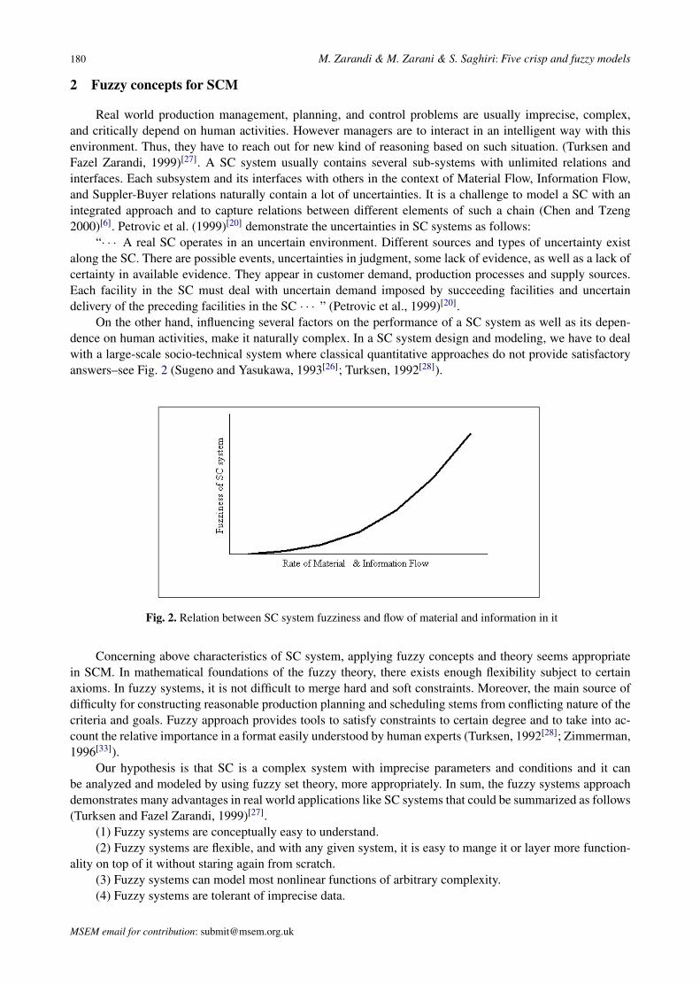
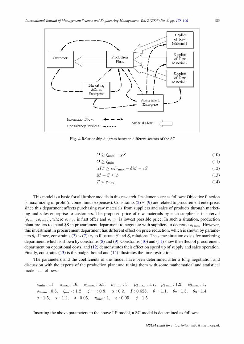
In this section, we develop several models for SC systems of an automotive industry. In these SC systemmodels, there exist 6 components, as shown in Fig. 3. The tasks of each enterprise, as shown in Fig. 4,are: customer, marketing and sales, manufacturing and assembly (production plant), purchasing (procuremententerprise), and parts and raw materials suppliers, where all of them are interconnected.

• The main focus of the research is on the role of marketing and procurement in selling and purchasingof goods in the SC, with a concentration on:

• The role of procurement enterprise in purchasing most proper raw materials, which directly affect theoperational costs of the production plant.

• The role of procurement enterprise in negotiations with suppliers on price, delivery, quality, etc.• The role of marketing enterprise in selling the product with the maximum possible price.• The role of procurement and marketing enterprises in finalizing a deal in minimum time. The stronger

actions of these two enterprise will lead to sails contract for production plant in a shorter time and accordinglythe investment costs of the production plant will be reduced.

Fig. 3. A schematic of the SC example

The goal of modeling the SC is maximization of profit in dollars. The variables and parameters of thesystem are as follows:

P : The price of final product;M : Costs to be paid by production plant in marketing sector;S: Costs to be paid by production plant in procurement sector;O: Operational costs of the production plant;T : Lead time of the arrangement until a contract is finalized with a customer;S1: Price of first raw material;S2: Price of second raw material;S3: Price of third raw material;πmin: The lowest price which is acceptable by production plant to sell its product;πmax: The maximum rate in which the product could be sold; Market situation dictate this rate.



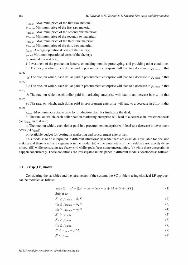
ρ1max: Maximum price of the first raw material;ρ1min: Minimum price of the first raw material;ρ2max: Maximum price of the second raw material;ρ2min: Minimum price of the second raw material;ρ3max: Maximum price of the third raw material;ρ3min: Minimum price of the third raw material;ζmed: Average operational costs of the factory;ζmin: Minimum operational costs of the factory;α: Annual interest rate;I: Investment of the production factory, on making moulds, prototyping, and providing other conditions;θ1: The rate, on which, each dollar paid in procurement enterprise will lead to a decrease in ρ1max in that

rate;θ2: The rate, on which, each dollar paid in procurement enterprise will lead to a decrease in ρ2max in that

rate;θ3: The rate, on which, each dollar paid in procurement enterprise will lead to a decrease in ρ3max in that

rate;β: The rate, on which, each dollar paid in marketing enterprise will lead to an increase in πmin in that

rate;χ: The rate, on which, each dollar paid in procurement enterprise will lead to a decrease in ζmed in that

rate;τmax: Maximum acceptable time for production plant for finalizing the deal;δ: The rate, on which, each dollar paid in marketing enterprise will lead to a decrease in investment costs

(αIτmax) in that rate;ε: The rate, on which, each dollar paid in a procurement enterprise will lead to a decrease in investment

costs (αIτmax);φ: Available budget for costing in marketing and procurement enterprises.This model is to be interpreted in different situations: (i) while there are exact data available for decision

making and there is not any vagueness in the model, (ii) while parameters of the model are not exactly deter-mined, (iii) while constraints are fuzzy, (iv) while goals faces some uncertainties, (v) while these uncertaintieshappen concurrently. These conditions are investigated in this paper in different models developed as follows:

3.1 Crisp (LP) model

Considering the variables and the parameters of the system, the SC problem using classical LP approachcan be modeled as follows:

max Z = P − [(S1 + S2 + S3) + S + M + O + αIT ] (1)

Subjet to:

S1 ≥ ρ1max − θ1S (2)

S2 ≥ ρ2max − θ2S (3)

S3 ≥ ρ3max − θ3S (4)

S1 ≥ ρ1min (5)

S2 ≥ ρ2min (6)

S3 ≥ ρ3min (7)

P ≤ πmin + βM (8)

P ≤ πmax (9)



Fig. 4. Relationship diagram between different sectors of the SC

O ≥ ζmed − χS (10)

O ≥ ζmin (11)

αIT ≥ αIτmax − δM − εS (12)

M + S ≤ φ (13)

T ≤ τmax (14)

This model is a basic for all further models in this research. Its elements are as follows: Objective functionis maximizing of profit (income minus expenses). Constraints (2) ∼ (9) are related to procurement enterprise,since this department affects purchasing raw materials from suppliers and sales of products through market-ing and sales enterprise to customers. The proposed price of raw materials by each supplier is in interval[ρi min, ρi max], where ρi max is first offer and ρi min is lowest possible price. In such a situation, productionplant prefers to spend $S in procurement department to negotiate with suppliers to decrease ρi max. However,this investment in procurement department has different effect on price reduction, which is shown by parame-ters θi. Hence, constraints (2) ∼ (7) try to illustrate S and Si relations. The same situation exists for marketingdepartment, which is shown by constrains (8) and (9). Constrains (10) and (11) show the effect of procurementdepartment on operational costs, and (12) demonstrates their effect on speed up of supply and sales operation.Finally, constrains (13) is the budget bound and (14) illustrates the time restriction.

The parameters and the coefficients of the model have been determined after a long negotiation anddiscussion with the experts of the production plant and tuning them with some mathematical and statisticalmodels as follows:

πmin : 11, πmax : 16, ρ1max : 6.5, ρ1min : 5, ρ2max : 1.7, ρ2min : 1.2, ρ3max : 1,

ρ3min : 0.5, ζmed : 1.2, ζmin : 0.8, α : 0.2, I : 0.625, θ1 : 1.1, θ2 : 1.3, θ3 : 1.4,

β : 1.5, χ : 1.2, δ : 0.05, τmax : 1, ε : 0.05, φ : 1.5

Inserting the above parameters to the above LP model, a SC model is determined as follows:



max Z = P − [(S1 + S2 + S3) + S + M + O + 0.125T ] (15)

Subject to :S1 ≥ 6.5− 1.1S (16)

S2 ≥ 1.7− 1.3S (17)

S3 ≥ 1− 1.4S (18)

S1 ≥ 5 (19)

S2 ≥ 1.2 (20)

S3 ≥ 0.5 (21)

P ≤ 11 + 1.5M (22)

P ≤ 16 (23)

O ≥ 1.2− 1.2S (24)

O ≥ 0.8 (25)

0.125T ≥ 0.125− 0.05M − 0.02S (26)

M + S ≤ 1.5 (27)

T ≤ 1 (28)

P,M,S,O, T, S1, S2, S3 ≥ 0 (29)

We used CPLEX software to solve this crisp linear program. The results of the model are shown in Tab.1.

Table 1. Solution of the crisp LP model

Var. Solution ($)Z 2.5364P 12.67S1 6.077S2 1.2S3 0.5M 1.115S 0.385O 0.8T 0.492

3.2 LP model with fuzzy coefficients

Real world situations are not often crisp. In this section, the former crisp LP model is modified to a fuzzyLP using fuzzy mathematics. For this purpose, we use both linguistic and nonlinguistic variables for gatheringdata from managers and decision makers of industry mentioned above. Thus, changing the linguistic variablesinto the language of the model, fuzzy numbers and fuzzy logic leads model designers to solve a realistic modelin comparison with the crisp LP model (Zimmermann, 1996)[33]. In the following subsections, first the crispmodel will be transferred to the model with fuzzy coefficients. Then, the situation in which bounds and goalsare fuzzy is considered. Finally, the above models will be merged into an aggregated fuzzy model with fuzzyobjectives, bounds and coefficient.

The linguistic input data of the model are transferred into fuzzy numbers. The procedure of this transfor-mation is as follows: First, a new interview has been carried out with associated experts. They were requestedto explain their ideas in more detail. At this stage, because there were additional explanations from the experts,the interviewer determined a wider range for each former crisp variable value. Upper and lower bounds of thisrange were extracted by the acquisition of all hidden points in the decision makers mind.



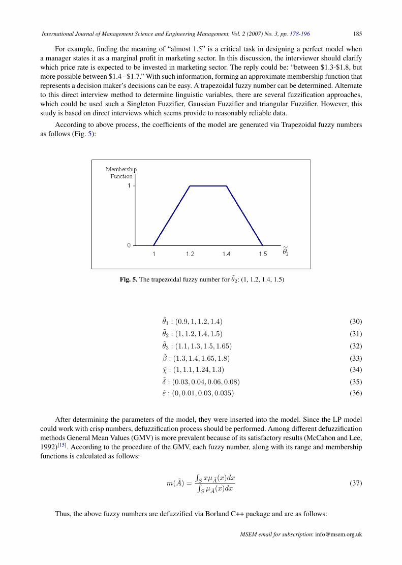
For example, finding the meaning of “almost 1.5” is a critical task in designing a perfect model whena manager states it as a marginal profit in marketing sector. In this discussion, the interviewer should clarifywhich price rate is expected to be invested in marketing sector. The reply could be: “between $1.3-$1.8, butmore possible between $1.4 –$1.7.” With such information, forming an approximate membership function thatrepresents a decision maker’s decisions can be easy. A trapezoidal fuzzy number can be determined. Alternateto this direct interview method to determine linguistic variables, there are several fuzzification approaches,which could be used such a Singleton Fuzzifier, Gaussian Fuzzifier and triangular Fuzzifier. However, thisstudy is based on direct interviews which seems provide to reasonably reliable data.

According to above process, the coefficients of the model are generated via Trapezoidal fuzzy numbersas follows (Fig. 5):

Fig. 5. The trapezoidal fuzzy number for θ2: (1, 1.2, 1.4, 1.5)

θ1 : (0.9, 1, 1.2, 1.4) (30)

θ2 : (1, 1.2, 1.4, 1.5) (31)

θ3 : (1.1, 1.3, 1.5, 1.65) (32)

β : (1.3, 1.4, 1.65, 1.8) (33)

χ : (1, 1.1, 1.24, 1.3) (34)

δ : (0.03, 0.04, 0.06, 0.08) (35)

ε : (0, 0.01, 0.03, 0.035) (36)

After determining the parameters of the model, they were inserted into the model. Since the LP modelcould work with crisp numbers, defuzzification process should be performed. Among different defuzzificationmethods General Mean Values (GMV) is more prevalent because of its satisfactory results (McCahon and Lee,1992)[15]. According to the procedure of the GMV, each fuzzy number, along with its range and membershipfunctions is calculated as follows:

m(A) =

∫S xµA(x)dx∫S µA(x)dx

(37)

Thus, the above fuzzy numbers are defuzzified via Borland C++ package and are as follows:



θ1 : (0.9, 1, 1.2, 1.4) = 1.13 (38)

θ2 : (1, 1.2, 1.4, 1.5) = 1.27 (39)

θ3 : (1.1, 1.3, 1.5, 1.65) = 1.38 (40)

β : (1.3, 1.4, 1.65, 1.8) = 1.54 (41)

χ : (1, 1.1, 1.24, 1.3) = 1.16 (42)

δ : (0.03, 0.04, 0.06, 0.08) = 0.053 (43)

ε : (0, 0.01, 0.03, 0.035) = 0.018 (44)

Next, the fuzzy LP model with fuzzy coefficient is formed as follows:

max Z := P − [(S1 + S2 + S3) + S + M + O + 0.125T (45)

Subject to :

S1 ≥ 6.5− 1.13S (46)

S2 ≥ 1.7− 1.27S (47)

S3 ≥ 1− 1.38S (48)

S1 ≥ 5 (49)

S2 ≥ 1.2 (50)

S3 ≥ 0.5 (51)

P ≤ 11 + 1.54M (52)

P ≤ 16 (53)

O ≥ 1.2− 1.16S (54)

O ≥ 0.8 (55)

0.125T ≥ 0.125− 0.053M − 0.018S (56)

M + S ≤ 1.5 (57)

T ≤ 1 (58)

Tab. 2 shows the solution of this model, where, it is rather improved in comparison to the crisp one. Thatis, while the value of Z in crisp model is equal to 2.54, in fuzzy LP it is 2.64 (Fig. 6).

Table 2. Solution of the LP model with defuzzified coefficients

Var. Solution ($)Z 2.64P 12.704S1 6.055S2 1.2S3 0.5M 1.106S 0.394O 0.8T 0.47

3.3 LP model with fuzzy bounds and objective function

In this section, we assume that the bounds and objective function of the model are fuzzy to examine thebehavior of the model.



Fig. 6. Schematic comparison between crisp LP model and LP model with defuzzified coefficients

LP models are generally stated in the following form:

max f(x) = z = cT x (59)

Subject to :Ax ≤ b (60)

x ≥ 0 (61)

c, x ∈ Rn, b ∈ Rm, A ∈ Rm×n (62)

Having fuzzy objective function G and fuzzy bounds C in variable space X , the fuzzy decision D canbe represented by (Bellman and Zadeh, 1970)[3]:

D = G ∩ C (63)

The “and” composition of goals and bounds should be interpreted as “logical and”, where, the “logicaland” corresponds to the set theoretic intersection (Zimmermann, 1996)[33]. The membership function of Dusing t-norm (Turksen and Fazel Zarandi, 1999[27]; Schweizer and Sklar, 1983[23]) is also as follows:

µD = t(µG, µC) (64)

It should be noted that the Zadeh’s standard t-norm is defined as µD = min(µG, µC). Hence, fuzzystructure of the model resulted from intersection of fuzzy objective functions and fuzzy constraints can berepresented by (Zimmermann, 1996)[33]:

Find x (65)

Subject to :

cT x≥z (66)

Ax≤b (67)

x ≥ 0 (68)

Substituting B =[−cT

A

]and d =

[zb

], the model is changed to



Find x (69)

Subject to :

BT x≥d (70)

x ≥ 0 (71)

Each rows of such a model could be represented by a fuzzy set with membership functionµi(x). Asindicated before, i.e., equation (63) and (64), the membership function of the “decision” represented by theintersection of fuzzy sets as follows (Schweizer and Sklar, 1983)[23]:

µD(x) = mini{µi(x)} (72)

Interpretation of µi(x) is not difficult. That is, when µi(x) is equal to 1 a constraint is completely satisfied,and when it is 0 the bound is totally not satisfied. Thus, µi(x) can be represented as follows:

µi(x) =

1 if Bix ≤ di

∈ [0, 1] if di ≤ Bix ≤ di + pi

0 if Bix ≥ di + pi

(73)

where, pi shows the degree to which the ith constraint could alter. When the membership functions are linear,then,

µi(x) =

1 if Bix ≤ di

1− Bix−dipi

if di ≤ Bix ≤ di + pi

0 if Bix ≥ di + pi

(74)

Now assuming λ to be mini{µi(x)}, the above model can be modified as follows (Zimmermann, 1996):

max λ (75)

Such that : λpi + Bix ≤ di + pi I = 1, · · · ,m + 1 (76)

x ≥ 0 (77)

Thus, our fuzzy SC model where the objective functions and constraints are fuzzy can be illustrated asfollows:

max λ (78)

Such that :

− 0.3λ + S1 ≥ 6.5− 1.1S − 0.3 (79)

− 0.1λ + S2 ≥ 1.7− 1.3S − 0.1 (80)

− 0.1λ + S3 ≥ 1− 1.4S − 0.1 (81)

− 0.2λ + S1 ≥ 5− 0.2 (82)

− 0.1λ + S2 ≥ 1.2− 0.1 (83)

− 0.1λ + S3 ≥ 0.5− 0.1 (84)

0.5λ + P ≤ 11 + 1.5M + 0.5 (85)

0.75λ + P ≤ 16 + 0.75 (86)

− 0.2λ + O ≥ 1.2− 1.2S − 0.2 (87)

− 0.2λ + O ≥ 0.8− 0.2 (88)

− 0.005λ + 0.125T ≥ 0.125− 0.05M − 0.02S − 0.005 (89)

0.3λ + M + S ≤ 1.5 + 0.3 (90)

0.3λ + T ≤ 1 + 0.3 (91)

− 0.2λ + P − S1 − S2 − S3 − M − S − O − 0.125T ≥ Z − 0.2 (92)



It should be noted that italic numbers in each row shows the tolerance of pi. Moreover, (92) is theobjective function of the crisp model, and Z (Solution) is considered to be 3.10 as a lower bound for it.

Therefore, the solution of the problem using CPLEX is shown in Tab. 3.As shown in Fig. 7, this solution shows an improvement obtained from former models.

Table 3. Solution of the LP model with fuzzy constraints and objective function

Var. Solution ($)Z 3.2P 13.067S1 5.95S2 1.16S3 0.458M 1.242S 3.846O 0.715T 0.4245λ 0.576

Z (Solution) 3.10

Fig. 7. Schematic comparison among crisp LP model, LP model with fuzzy coefficient, and LP with fuzzy constraintsand objective function

3.4 LP model with fuzzy coefficients, bounds and objective function

In this section, all of the parameters and constraints of the LP model are assumed to be fuzzy. Theprocedure for the development this model is as follows:

Step 1. Construct the crisp model (as shown in section 3.1).Step 2. Fuzzify of the coefficients of the crisp model (as shown in section 3.2).Step 3. Transfer the last model to a decision making by intersecting objective function with bounds (as

shown in section 3.3).Step 4. Solving the model.



Thus, following the explained step-by-step procedures in section 3.1, 3.2 and 3.3, the final LP model withfuzzy coefficient and constraints can be easily developed as follows:

max λ (93)

Such that :

− 0.3λ + S1 ≥ 6.5− 1.1S − 0.3 (94)

− 0.1λ + S2 ≥ 1.7− 1.3S − 0.1 (95)

− 0.1λ + S3 ≥ 1− 1.4S − 0.1 (96)

− 0.2λ + S1 ≥ 5− 0.2 (97)

− 0.1λ + S2 ≥ 1.2− 0.1 (98)

− 0.1λ + S3 ≥ 0.5− 0.1 (99)

0.5λ + P ≤ 11 + 1.5M + 0.5 (100)

0.75λ + P ≤ 16 + 0.75 (101)

− 0.2λ + O ≥ 1.2− 1.2S − 0.2 (102)

− 0.2λ + O ≥ 0.8− 0.2 (103)

− 0.005λ + 0.125T ≥ 0.125− 0.05M − 0.02S − 0.005 (104)

0.3λ + M + S ≤ 1.5 + 0.3 (105)

0.3λ + T ≤ 1 + 0.3 (106)

− 0.2λ + P − S1 − S2 − S3 − M − S − O − 0.125T ≥ Z − 0.2 (107)

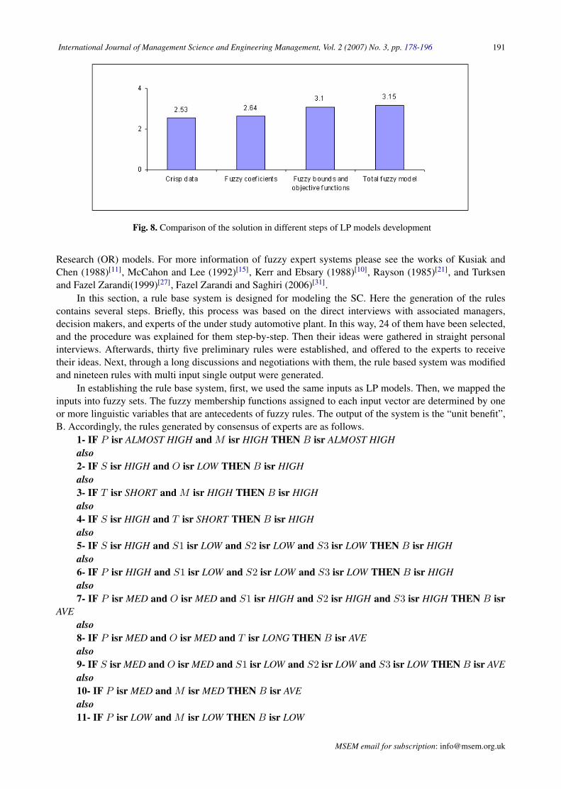
As shown in Tab. 4, the Z (Solution) in this case is equal to 3.154, which has been rather improved incomparison to previous models. The comparison of the solution of different LP models is shown in Fig. 8.

Table 4. Solution of the LP model with fuzzy coefficients, constraints, and objective function

Var. Solution ($)Z 3.2 (as an input)P 13.075S1 5.94S2 1.16S3 0.46M 1.2S 0.39O 0.72T 0.41λ 0.614

Z (Solution) 3.154

This improvement in development of the fuzzy models has several advantages, such as clear benefit insimplifying data gathering and works with linguistic variables. This creates flexibility in model building. Inthis way, more realistic representation of system behavior is also obtained by the introduction of tolerances.

3.5 Fuzzy expert system model for SC

In this section, we first develop a new fuzzy expert system based on rule bases for SC. Then, we comparethe result with those of former crisp and fuzzy LPs developed for SC.

The main problems with mathematical models are their complexity and inability to use natural languages(Turksen, 1992)[28]. Fuzzy expert systems are valuable tools to come up with these problems of Operation



Fig. 8. Comparison of the solution in different steps of LP models development

Research (OR) models. For more information of fuzzy expert systems please see the works of Kusiak andChen (1988)[11], McCahon and Lee (1992)[15], Kerr and Ebsary (1988)[10], Rayson (1985)[21], and Turksenand Fazel Zarandi(1999)[27], Fazel Zarandi and Saghiri (2006)[31].

In this section, a rule base system is designed for modeling the SC. Here the generation of the rulescontains several steps. Briefly, this process was based on the direct interviews with associated managers,decision makers, and experts of the under study automotive plant. In this way, 24 of them have been selected,and the procedure was explained for them step-by-step. Then their ideas were gathered in straight personalinterviews. Afterwards, thirty five preliminary rules were established, and offered to the experts to receivetheir ideas. Next, through a long discussions and negotiations with them, the rule based system was modifiedand nineteen rules with multi input single output were generated.

In establishing the rule base system, first, we used the same inputs as LP models. Then, we mapped theinputs into fuzzy sets. The fuzzy membership functions assigned to each input vector are determined by oneor more linguistic variables that are antecedents of fuzzy rules. The output of the system is the “unit benefit”,B. Accordingly, the rules generated by consensus of experts are as follows.

1- IF P isr ALMOST HIGH and M isr HIGH THEN B isr ALMOST HIGHalso2- IF S isr HIGH and O isr LOW THEN B isr HIGHalso3- IF T isr SHORT and M isr HIGH THEN B isr HIGHalso4- IF S isr HIGH and T isr SHORT THEN B isr HIGHalso5- IF S isr HIGH and S1 isr LOW and S2 isr LOW and S3 isr LOW THEN B isr HIGHalso6- IF P isr HIGH and S1 isr LOW and S2 isr LOW and S3 isr LOW THEN B isr HIGHalso7- IF P isr MED and O isr MED and S1 isr HIGH and S2 isr HIGH and S3 isr HIGH THEN B isr

AVEalso8- IF P isr MED and O isr MED and T isr LONG THEN B isr AVEalso9- IF S isr MED and O isr MED and S1 isr LOW and S2 isr LOW and S3 isr LOW THEN B isr AVEalso10- IF P isr MED and M isr MED THEN B isr AVEalso11- IF P isr LOW and M isr LOW THEN B isr LOW



also12- IF S isr LOW and O isr HIGH and S1 isr HIGH and S2 isr HIGH and S3 isr HIGH THEN B

isr LOWalso13- IF P isr LOW and O isr MED and T isr LONG THEN B isr LOWalso14- IF P isr LOW and S1 isr HIGH and S2 isr HIGH and S3 isr HIGH THEN B isr LOWalso15- IF P isr LOW and O isr HIGH THEN B isr LOWalso16- IF S isr LOW and T isr LONG THEN B isr ALMOST LOWalso17- IF S1 isr HIGH and S2 isr HIGH and S3 isr HIGH THEN B isr LOWalso18- IF P isr ALMOST HIGH and M isr HIGH and T isr SHORT THENB isr ALMOST HIGHalso19- IF S isr HIGH and O isr ALMOST LOW and T isr SHORT and S1 isr LOW and S2 isr LOW and

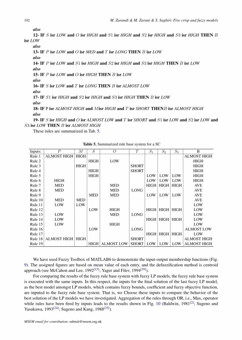
S3 isr LOW THEN B isr ALMOST HIGHThese rules are summarized in Tab. 5.

Table 5. Summarized rule base system for a SC

Inputs: P M S O T S1 S2 S3 BRule 1 ALMOST HIGH HIGH ALMOST HIGHRule 2 HIGH LOW HIGHRule 3 HIGH SHORT HIGHRule 4 HIGH SHORT HIGHRule 5 HIGH LOW LOW LOW HIGHRule 6 HIGH LOW LOW LOW HIGHRule 7 MED MED HIGH HIGH HIGH AVERule 8 MED MED LONG AVERule 9 MED MED LOW LOW LOW AVERule 10 MED MED AVERule 11 LOW LOW LOWRule 12 LOW HIGH HIGH HIGH HIGH LOWRule 13 LOW MED LONG LOWRule 14 LOW HIGH HIGH HIGH LOWRule 15 LOW HIGH LOWRule 16 LOW LONG ALMOST LOWRule 17 HIGH HIGH HIGH LOWRule 18 ALMOST HIGH HIGH SHORT ALMOST HIGHRule 19 HIGH ALMOST LOW SHORT LOW LOW LOW ALMOST HIGH

We have used Fuzzy Toolbox of MATLAB6 to demonstrate the input-output membership functions (Fig.9). The assigned figures are based on mean value of each entry, and the defuzzification method is centroidapproach (see McCahon and Lee, 1992[15]; Yager and Filev, 1994[29]).

For comparing the results of the fuzzy rule base system with fuzzy LP models, the fuzzy rule base systemis executed with the same inputs. In this respect, the inputs for the final solution of the last fuzzy LP model,as the best model amongst LP models, which contains fuzzy bounds, coefficient and fuzzy objective function,are inputed to the fuzzy rule base system. That is, we Choose these inputs to compare the behavior of thebest solution of the LP models we have investigated. Aggregation of the rules through OR, i.e., Max, operatorwhile rules have been fired by inputs leads to the results shown in Fig. 10 (Baldwin, 1981[2]; Sugeno andYasukawa, 1993[24]; Sugeno and Kang, 1988[25]).



Fig. 9. Graphical view of the rule base system

Fig. 10. Result of the rule base system with the inputs which were solution of the LP model

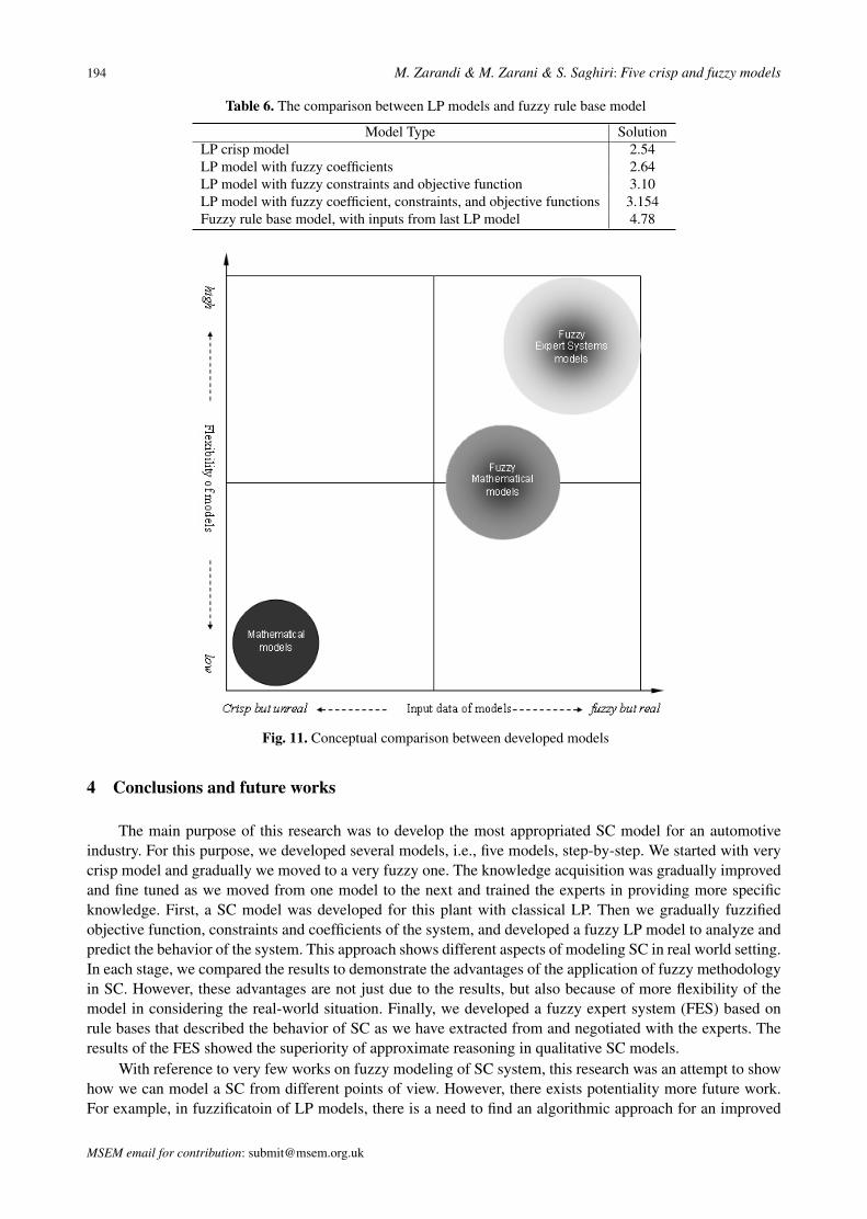
As shown in Tab. 6, while the result of fuzzy LP is 3.154, the result of fuzzy expert system is 4.78, whichis result of considering real situatoin. Tab. 6 represents comparison between all results, produced by differentmethods. Furthermore, Fig. 11, illustrates a schematic comparison between these models.



Table 6. The comparison between LP models and fuzzy rule base model

Model Type SolutionLP crisp model 2.54LP model with fuzzy coefficients 2.64LP model with fuzzy constraints and objective function 3.10LP model with fuzzy coefficient, constraints, and objective functions 3.154Fuzzy rule base model, with inputs from last LP model 4.78

Fig. 11. Conceptual comparison between developed models

4 Conclusions and future works

The main purpose of this research was to develop the most appropriated SC model for an automotiveindustry. For this purpose, we developed several models, i.e., five models, step-by-step. We started with verycrisp model and gradually we moved to a very fuzzy one. The knowledge acquisition was gradually improvedand fine tuned as we moved from one model to the next and trained the experts in providing more specificknowledge. First, a SC model was developed for this plant with classical LP. Then we gradually fuzzifiedobjective function, constraints and coefficients of the system, and developed a fuzzy LP model to analyze andpredict the behavior of the system. This approach shows different aspects of modeling SC in real world setting.In each stage, we compared the results to demonstrate the advantages of the application of fuzzy methodologyin SC. However, these advantages are not just due to the results, but also because of more flexibility of themodel in considering the real-world situation. Finally, we developed a fuzzy expert system (FES) based onrule bases that described the behavior of SC as we have extracted from and negotiated with the experts. Theresults of the FES showed the superiority of approximate reasoning in qualitative SC models.

With reference to very few works on fuzzy modeling of SC system, this research was an attempt to showhow we can model a SC from different points of view. However, there exists potentiality more future work.For example, in fuzzificatoin of LP models, there is a need to find an algorithmic approach for an improved



representation of such models. Also in this paper we used several heuristic approaches for rule generation. Forthis purpose, the application of other approaches such as Neural Networks and/or fuzzy clustering algorithmsmay produce better results.

References

[1] E. Alexander. Improving marketing/logistics cross-functional collaboration in the supply chain. Industrial Mar-keting Management, 2000, 29(1): 86–97.

[2] J. Baldwin. Fuzzy Logic Knowledge Basis and Automated Fuzzy Reasoning. Lasker, 1981.[3] B. Bellman, L. Zadeh. Decision making in fuzzy environment. Management Science, 1970, 141–164.[4] J. Bloemhof-Ruwaard, P. V. Beek, et. al. Interaction between operational research and environmental management.

European Journal of Operation Research, 1995, 85(2): 229–243.[5] P. Chandra, M. Fisher. Coordination of production and distribution planning. European Journal of Operational

Research, 1994, 72(3): 503–517.[6] Y. Chen, G. Tzeng. Fuzzy multi-objective approach to the supply chain model. International Journal of Fuzzy

Systems, 2000, 2(3): 220–228.[7] Y. Gerchak. On the allocation of uncertainty-reduction effort to minimize total variability. IIE Transactions, 2000.[8] Q. He, E. Jewkes. Performance measure of a making-to-order inventory-production system. in: IIE Transactions,

2000.[9] J. Heide, G. John. Alliances in industial purchasing: Determinants of joint action in buyer-supplier relationships.

Journal of Marketing, 1990, 27(1): 24–36.[10] R. Kerr, R. Ebsary. Implementation of an expert system for production scheduling. European Journal of Opera-

tional Research, 1988, 33: 17–29.[11] A. Kusiak, M. Chen. Expert systems for planning and scheduling manufacturing systems. European Journal of

Operational Research, 1988, 34: 113–130.[12] R. Lancioni. New developments in supply chain management for millennium. Industrial Marketing Management,

2000, 29(1): 1–6.[13] R. Lancioni, M. Smith. The role of the internet in supply chain management. Industrial Marketing Management,

2000, 29(1): 45–46.[14] X. Lui. Performance analysis and optimization of supply networks (manufacturing and inventory control). in:

Hong Kong University of SCI and TECH, 1999.[15] C. McCahon, E. Lee. Fuzzy job sequencing for a flow shop. European Journal of Operational Research, 1992, 62:

294–301.[16] M. Monczka, K. Peterson, et. al. Success factors in strategic supplier alliances: The buying company perspective.

Decision Sciences, 1998, 29(3): 53–78.[17] R. Mullins. Expansion of logistics services adds to liability for operators. Journal of Commerce, 1999.[18] K. Ohmae. The global logic of strategic aliances. in: Harvard Business Review, 1989, 143–154.[19] D. Petrovic, R. Dobrila, et. al. Modeling and simulation of a supply chain in an uncertain environment. European

Journal of Operational Research, 1998, (1).[20] D. Petrovic, R. Dobrila, et. al. Supply chain modeling using fuzzy sets. International Journal of Production

Economics, 1999.[21] P. Rayson. A review of expert systems principles and their role in manufacturing systems. Robotica, 1985, 3:

279–287.[22] R. Samroengraja. Staggered ordering policies for twe-echelon production/distribution systems. 1999. Columbia

University.[23] B. Schweizer, A. Sklar. Probablistic metric space. North-Holland, 1983.[24] F. Stuart. Supplier partnerships: Influencing factors and strategic benfits. Internation Journal of Purchasing and

Material Management, 1993, 29(4): 22–28.[25] M. Sugeno, G. Kang. Structure identification of fuzzy model. Fuzzy Set and Systems, 1988, 28: 15–33.[26] M. Sugeno, T. Yasukawa. A fuzzy-logic-based approach to qualitative modeling. IEEE Transaction on Fuzzy

Systems, 1993, 1(1): 7–31.[27] I. Turksen, M. Zarandi. Production planning and scheduling: Fuzzy and crisp approaches. Practical Applications

of Fuzzy Technologies, 1999, 479–529.[28] T. Turksen. Fuzzy expert systems for ie/or/ms. Fuzzy Sets and Systems, 1992, 51: 1–27.[29] R. Yager, D. Filev. Essentials of fuzzy modeling and control. 1994.[30] M. Zarandi, S. Saghiri. A comprehensive fuzzy multi-objective model for supplier selection process. in: Proceed-

ing of the IEEE International Conference on Fuzzy Systems, USA, 2003, 25–28.



[31] M. Zarandi, S. Saghiri. Developing fuzzy expert systems models for supply cahin complex problem: A comparisonwith linear programming. 2006 IEEE World Congress on Computational Intelligence, Canada, 2006.

[32] M. Zarandi, I. Turksen, S. Saghiri. Supply chain: Crisp and fuzzy aspects. International Journal of Applied Math& Computter Science, 2002, 12(3): 423–435.

[33] H. Zimmermann. Fuzzy Set Theory and its Applications. Kluwer Academic Publishers, 1996.


Five crisp and fuzzy models for supply chain of an ... crisp and fuzzy models for supply chain of an...

Documents

Transcript of Five crisp and fuzzy models for supply chain of an ... crisp and fuzzy models for supply chain of an...