Supervisor: Dr. Anders Brandt Examiners: Prof. Anders Östman - Dr. Bo Malmström

DEPARTMENT OF TECHNOLOGY AND BUILT ENVIRONMENT

Comparison of fuzzy and crisp analytic

hierarchy process (AHP) methods for spatial

multicriteria decision analysis in GIS

Maryam Kordi

September 2008

Master’s Thesis in Geomatics

Abstract There are a number of decision making problems in which Geographical Information System (GIS) has employed to organize and facilitate the procedure of analyzing the problem. These GIS-based decision problems which typically include a number of different criteria and alternatives are generally analyzed by Multicriteria Decision Analysis (MCDA).Different locations within a geographical area represent the alternatives by which the overall goal of the project is achieved. The quality of achieving the goal is evaluated by a set of criteria which should be considered in the work. Analytic Hierarchy Process (AHP) which is a powerful method of MCDA generally can organize spatial problems and decides which alternatives are most suitable for the defined problems. However due to some intrinsic uncertainty in the method, a number of authors suggest fuzzifying the method while others are against fuzzification of the AHP.

The debate over fuzzifying AHP is going on and attempt for finding that was mostly in theory, and little, if any; practical comparison between the AHP and fuzzified AHP has done. This work presents a practical comparison of AHP and fuzzy AHP in a GIS-based problem, case study, for locating a dam in Costa Rica, considering different criteria. In order to perform the AHP and fuzzy AHP in the GIS-based problem and calculating weights of the criteria by the methods, some computer codes have written and developed in MATLAB.

The comparisons between the AHP and fuzzy AHP methods are done on result weights and on the result final maps. The comparison between the weights is repeated on different levels of uncertainty in fuzzy AHP then all the results are compared with the result of AHP method. Also this study for checking the effect of fuzzification on results is suggested Chi-Square test as a suitable tool.

Comparisons between the resulting weights of the AHP and fuzzy AHP methods show some differences between the methods. Furthermore, the Chi-Square test shows that the higher level of uncertainty in the fuzzy AHP, the greater the difference in results between the AHP and fuzzy AHP methods.

Keywords: Geographical Information System (GIS), Multicriteria Decision Analysis (MCDA), Analytic Hierarchy Process (AHP).

1

Preface

This thesis is dealing with geographical information system and multicriteria decision analysis. These two areas of research are very interesting to me as my academic background was in Applied Mathematics and Geomatics.

Having a contact with Thomas L. Saaty and Jacek Malczewski, they sent me some related articles that encouraged me to focus on fuzzifying the AHP concept.

According to some natural uncertainty in the AHP, some researchers have used the fuzzy concept to fuzzify the method while other researchers are against it. So far most attempts for fuzzifying the AHP and comparing the fuzzy result with result of AHP have been made in theory and almost no practical examples have been performed. Lack of practical approach in this field, led me to define a practical example of a GIS-based decision making problem. This example was based on a project course where the task was to find the optimum location for a dam in Costa Rica, which I did during my Master studies.

I would like to dedicate this work to my parents in Iran for always supporting and believing in me. Also special thanks go to my sister Masoumeh and my brother in law Hesam who encouraged me to pursue my graduate studies in Sweden. I am also grateful for their help and support when I was in Uppsala, without their help I could not have started my studies comfortably.

I would like to thank my supervisor Anders Brandt for his encouragement from the beginning and enthusiastic support throughout the thesis. I can never thank him enough for his academic support and help, not only in my Master’s thesis but in all the steps of my studies in University of Gävle.

Thanks are due to Stig-Göran Mårtensson, Anders Östman, Pia Ollert-Hallqvist, Peter Fawcett, Lise-Lotte Dahlberg and Bo Malmström because they were great teachers for me during my master study.

For their help in finding the interesting subject for my Master’s thesis and sending me some invaluable articles, Thomas L. Saaty and Jacek Malczewski must be thanked.

I would like to thank Mehdi Ardavan for his help during my thesis work, also for editing and revising my thesis report and MATLAB codes.

I also would like to thank all Personnel in the division of Geomatics in University of Gävle especially Staffan Nygren who helped me with some computer problems and also thanks are due to my friends in the devision Anna Hansson, Ulrika Lindgren and Linda Alm for being the best friends possible.

Also thanks are due to Maryam Mohammadi for her help in preparing some of the figures and Willem Tims for revising some part of my report, also due to Tayyab Hussain and Ioannis Tolikas for helping me with some GIS-software problems at the beginning of the work.

2

Table of contents

Abstract ............................................................................................................................................... 1

Preface................................................................................................................................................. 2

Table of contents .................................................................................................................................. 3

1. Introduction .................................................................................................................................. 5

2. Multicriteria Decision Analysis (MCDA)....................................................................................... 6

2.1. Analytic Hierarchy Process (AHP).............................................................................................. 6

2.2. Calculating weights .................................................................................................................... 8

2.3. Mean of normalized values - Lambda max method ..................................................................... 8

2.4. Geometric mean method............................................................................................................. 8

2.5. Consistency ratio in the AHP ...................................................................................................... 9

2.6. Uncertainty in the AHP .............................................................................................................. 9

2.7. Fuzzy weights .......................................................................................................................... 10

2.8. Consistency ratio in fuzzifying the pairwise ratios ..................................................................... 10

2.9. Employing geometric mean for fuzzy weights ........................................................................... 10

3. Material and method ................................................................................................................... 12

3.1. Study area ................................................................................................................................ 12

3.2. Hydrological modeling ............................................................................................................. 14

3.3. Stream network ........................................................................................................................ 14

3.4. Hydraulic head......................................................................................................................... 15

3.5. Undulation ............................................................................................................................... 15

3.6. Criteria in GIS-MCDA ............................................................................................................. 15

3.7. Factors of Forest and Agriculture .............................................................................................. 16

3.8. Factors of Road and City .......................................................................................................... 17

3.9. Factors of Hydraulic head, Water discharge and Undulation ...................................................... 17

3.10. Constraints in GIS-MCDA...................................................................................................... 17

3

3.11. Constraint of River ................................................................................................................. 18

3.12. Constraints of Reservoir and National Park ............................................................................. 18

3.13. Multicriteria Decision Making in GIS ..................................................................................... 19

3.14. Consistency ratio.................................................................................................................... 22

3.15. Defuzzification....................................................................................................................... 23

4. Results ........................................................................................................................................... 24

4.1. AHP Lambda Max (λmax) .......................................................................................................... 24

4.2. AHP geometric mean ............................................................................................................... 25

4.3. AHP fuzzy triangular................................................................................................................ 26

4.4. AHP fuzzy narrow trapezoidal .................................................................................................. 27

4.5. AHP fuzzy medium trapezoidal ................................................................................................ 28

4.6. AHP fuzzy wide trapezoidal ..................................................................................................... 29

4.7. Percentage difference between weights ..................................................................................... 30

4.8. Chi-Square ( ) test for Independence...................................................................................... 31 2χ

4.9. Comparison between maps ....................................................................................................... 33

5. Discussions and Conclusion ............................................................................................................ 36

References ......................................................................................................................................... 37

Appendix A........................................................................................................................................ 39

Appendix B. ....................................................................................................................................... 40

Appendix C........................................................................................................................................ 45

4

1. Introduction

GIS-based multicriteria decision analysis (GIS-MCDA) is a process of decision making at which geographical data and value judgments are brought together to obtain more information for the decision makers (Malczewski 2006).

Although Analytic Hierarchy Process (AHP) method is a powerful tool in MCDA for spatial problems, some of the researchers believe that the Saaty’s AHP method has some weaknesses. For example as Yang and Chen (2004) have mentioned, the uncertainty associated with the mapping of decision makers judgment to number, is not taken into account by the AHP and also the preference and personal judgment of decision maker have huge effect on the AHP result.

In order to overcome these problems, some researchers and authors made the Saaty’s AHP modified and fuzzified to formulate and control the uncertainty. E.g. Buckley (1985) has considered trapezoidal membership function for comparison ratios in AHP and Chang (1996) has developed a new approach for triangular case. In fact they believe having a defined uncertainty in the form of fuzzy numbers in comparison ratios and then obtaining the weights in fuzzy forms, help the decision-makers to get a better understanding of the final importance of the factors and the uncertainty lying within them.

However, Saaty, the developer of the AHP, is against fuzzification of his method. He believes the AHP by pairwise comparison matrix is already fuzzy because some uncertainty lies in the nature of the method, i.e. he believes that ratios in the method are not absolute or crisp numbers, in fact they are fuzzy numbers, so making the AHP fuzzier not only does not guarantee better results but could make it worse (Saaty & Tran 2007, 2008; Saaty 2008).

So far the attempts and works for comparing the AHP and fuzzy AHP were mostly done in theory and almost not enough practical examples of a GIS-based decision making problem has been done. The main goal of this thesis is to practically compare the results of AHP and fuzzy AHP methods by applying them in a GIS based problem.

In order to practically analyze the probable difference in result of performing AHP and fuzzy AHP methods, in a sophisticated example which is based on GIS, the optimum site for a dam is located and analyzed. The dam is to be investigated over two main upstream tributaries of Reventazon River in Costa Rica, considering different criteria. The comparison between the result of AHP and fuzzy AHP in the work is done in two approaches.

The first comparison approach is done on weights obtained from the AHP and fuzzy AHP methods. Analysis is carried out first in normal and non-fuzzy numbers and then fuzzified AHP is applied on fuzzy comparison ratios which yield weights in fuzzy format. In the fuzzy AHP, pairwise comparison matrix is considered with different degrees of uncertainty for ratios which has not been considered in previous works in this field. For calculating weights of AHP and fuzzy AHP and performing the methods, some computer programs have been created and developed by the author in MATLAB.

The second comparison approach is done in order to analyze the probable difference in the resulted maps from GIS software after performing the AHP and fuzzy AHP methods. Also, this thesis for checking the effect of fuzzification on result maps, suggest and perform the Chi-Square test as a suitable tool. The Chi-Square test, statistically checks the effect of fuzzification on GIS resulted maps in terms of the degree of uncertainty in fuzzy weights. Such a comparison between the AHP and fuzzy AHP, which is based on GIS maps, has not been done in this format before.

5

2. Multicriteria Decision Analysis (MCDA)

Multicriteria decision analysis (MCDA) for structuring decision problem and evaluating alternatives provides a rich collection of methods (Malczewski 2006). In most management and decision-making problems the management team has already a well-defined goal that must be achieved. In order to reach that aim always it is necessary to choose from a number of options. These options, in the field of the MCDA, are referred to as alternatives.

The decision makers or the decision-makers consider the existing alternatives which have different attributes and characteristics and the final job is to choose the best among them. Choosing among the alternatives is done by considering the impact of these alternatives on the quality of the final result alongside with shortcomings of every alternative. Therefore effects of alternatives on different issues such as environmental issues, financial matters or cost and benefit considerations, social considerations, technical problems, etc give rise to consideration of several criteria which play important roles in finalizing the project.

However, the criteria demonstrate the characteristics and important issues which the final goal is evaluated according to them. If a decision maker wants to rank the importance of the alternatives, this only is according to the criteria. But it should be noticed that according to every different criteria the ranking between the alternatives would be different.

For applying MCDA, a tool is needed which takes the ranking and comparison data to processes them and calculates the weights of different alternatives or criteria. The AHP can be served as a powerful tool in calculating weights and pursuing MCDA procedure.

2.1. Analytic Hierarchy Process (AHP)

The AHP which is a powerful tool in applying MCDA was introduced and developed by Saaty in 1980. In the AHP method, obtaining the weights or priority vector of the alternatives or the criteria is required. For this purpose Saaty (1980) has used and developed the Pairwise Comparison Method (PCM), which is explained in detail in next part of the work.

In the AHP the decision making process starts with dividing the problem into a hierarchy of issues which should be considered in the work. These hierarchical orders help to simplify the illustration of the problem and bring it to a condition which is more easily understood. In each hierarchical level the weights of the elements are calculated. The decision on the final goal is made considering the weights of criteria and alternatives.

In Figure 1, where the structure of AHP elements is illustrated, it is shown that the goal is decided through a number of different criteria. These criteria determine the quality of achieving the goal using any of Alternatives ( , i=1... k). The are different options, choices or alternatives that could be used to reach the final aim of the project. Comparing these alternatives and defining their importance over each other are done using the pairwise comparison method. Giving importance ratios for each pair of alternatives, a matrix of pairwise comparison ratios is obtained.

iA iA

6

Figure 1. Structure of the AHP.

The criteria might also have different importance compared to each other. Therefore a pairwise comparison matrix is considered for the criteria. Elements of this matrix are pairwise or mutual importance ratios between the criteria which are decided on the basis that how well every criterion serves and how important it is in reaching the final goal.

For creating the pairwise comparison matrix in the PCM, Saaty (1980) has employed a system of numbers to indicate how much one criterion is more important than the other. These numerical scale values and their corresponding intensities are stated in Table 1.

Table 1. Scales in pairwise comparisons (Adapted from Saaty 1980).

Intensity of importance Verbal judgment of preference

1 Equally Importance

3 Moderate importance

5 Strong importance

7 Extreme importance

9 Extremely more important

2, 4, 6, 8 Intermediate values between adjacent scale values

In order to compare homogeneous elements whose comparison falls within one unit, decimals are used (Saaty 2006). If the elements of the pairwise comparison matrix are shown with , which indicates the importance of i’th criterion over j’th, then could be calculated as 1/ (Boroushaki & Malczewski 2008).

ijc

jic ijc

The AHP method employs different techniques to determine the final weights; two of them are explained and used in his thesis. The first is Lambda Max ( maxλ ) technique and the other is geometric mean. Later, in Result chapter, it is shown that different techniques in the AHP do not yield the same result.

A1 A2

A3

AK

GOAL

A1 A2

A3

AK

Criterion 1 Criterion 2

A1A2

A3

AK

Criterion 3

A1A2

A3

AK

Criterion k

7

2.2. Calculating weights

Saaty (1980) has used the lambda max technique to obtain the weights of the criteria in the pairwise comparison method. Every matrix has a set of eigenvalues and for every eigenvalue there is a corresponding eigenvector. In Saaty’s lambda max technique, a vector of weights is defined as the normalized eigenvector corresponding to the largest eigenvalue λmax. If the weights are shown as a vector w consisted of wi (i=1…n), then the following formula shows how they are calculated.

C × w = λ × w (1)

at which C is the pairwise comparison matrix of the criteria; w is the vector of weights and λ is the eigenvalue that in this method should be the maximum of them, i.e. maxλ .

In this method special mathematical conditions are required to guarantee that a unique answer is yielded. Also difficulties in calculating and finding the eigen values and vectors have led to use of an approximation to the lambda max method. As Malczewski (1999) used in his book an approximation of the eigenvector associated with the maximum eigenvalue is calculated through a simple procedure which is sometimes referred to as mean of normalized values.

2.3. Mean of normalized values – Lambda max method

In mean of normalized values method which gives an approximation of lambda max method, the sum of elements in each column in pairwise comparison matrix is calculated. Then each column elements is divided by the calculated sum at the previous step. Then the arithmetic average of each row of the normalized matrix gives the weight of the corresponding criterion or alternative. The accuracy of this approximation is increased when the pairwise comparison matrix has a low consistency ratio.

2.4. Geometric mean method

Another method of calculating the weights of criteria in the PCM is geometric mean method. In this method as Buckley (1985) explained, the weights in a pairwise comparison matrix of alternatives, , are calculated by following formula.

A

( )∏=

=n

1j

n/1iji ar (2)

and then ∑

=

jj

ii r

rw (3)

at which (i,j=1..n) are the comparison ratios in the pairwise comparison matrix and n is number of alternatives.

ija

8

2.5. Consistency ratio in the AHP

A matrix A is called consistent if and only if ijkjik aa.a = at which is the ij’th element of the matrix (Buckley 1985). However in practice it is unrealistic to expect the decision-makers provide pairwise comparison matrices which are exactly consistent especially in the cases with a large number of alternatives. Expressing the real feelings of the decision makers generally lead to matrices that are not quite consistent. However some matrices might violate consistency very slightly by only two or three elements while others may have values that cannot even be called close to consistency.

ija

A measure of how far a matrix is from consistency is performed by Consistency Ratio (C.R.). Han and Tsay (1998) explained that having the value of maxλ is required in calculating the consistency ratio. This is obtained by calculating matrix product of the pairwise comparison matrix and the weight vectors and then adding all elements of the resulting vector. After that a Consistency Index ( ) is introduced as: .I.C

1nn.I.C max

−−λ

= (4) at which n is the number of criteria and maxλ is the biggest eigenvalue (Han & Tsay 1998; Malczewski 1999).

Random Index (R.I.) is the consistency index of a pairwise comparison matrix which is generated randomly. Random index depends on the number of elements which are compared and as it is shown in Table 2; in each case for every n, the final R.I. is the average of a large numbers of R.I. calculated for a randomly generated matrix. The final consistency ratio is calculated by comparing the C.I. with the Random Index (Malczewski 1999).

.I.R

.I.C.R.C = (5)

The consistency ratio is designed such a way that shows a reasonable level of consistency in the pairwise comparisons if < 0.10 and indicate inconsistent judgments. .R.C 10.0.R.C ≥

Table 2. Random Inconsistency Index (RI) for n = 1, 2,…, 12 (Adapted from Saaty 1980).

n 1 2 3 4 5 6 7 8 9 10 11 12

R.I. 0.00 0.00 0.58 0.90 1.12 1.24 1.32 1.41 1.45 1.49 1.51 1.48

2.6. Uncertainty in the AHP

As it has already been stated in the introduction, Saaty (2008) believes that some uncertainty is lying in the nature of AHP method. Also Buckley (1985) has raised questions about certainty of the comparison ratios used in the AHP. He had considered a situation in which the decision-maker can express feelings of uncertainty while he/she is ranking or comparing different alternatives or criteria. The method he has used to take uncertainties into account is using fuzzy numbers instead of crisp numbers in order to compare the importance between the alternatives or criteria.

9

2.7. Fuzzy weights

As Buckley (1985) has considered, trapezoidal membership functions is adopted for fuzzy numbers in this work to fuzzify the comparison ratios. In specific cases, by selecting accordingly the parameters of membership function, trapezoidal shape is converted to triangular.

Suppose that the a fuzzy number is described as (α,β,γ,δ) where 0<α≤β≤γ≤δ and at which α, β, γ and δ are the four parts of the fuzzy number, the membership function for any given fuzzy number is shown by μ(x) and these two numbers form an ordered pair (x, μ(x)). The description of fuzzy number means that the membership function is 0 to the left of α. Then a line connects the two points (α, 0) and (β, 1). After that it is constant at value 1 between β and γ. Then a line connect the two points (γ, 1) and (δ, 0) and finally membership function equals zero in the right of δ. Figure 2 illustrates a fuzzy membership function of a fuzzy number.

A corresponding fuzzy ratio of is shown with a bar sign above it i.e. ija ),,,(a ijijijijij δγβα= . So from now on, the bar sign above a variable, means that it is fuzzy.

Figure 2. Fuzzy memberships function of a fuzzy number.

2.8. Consistency ratio in fuzzifying the pairwise ratios

Buckley (1985) has proved the following theorem:

Consider ]a[ ijA = where ),,,(a ijijijijij δγβα= and let ijijij a γ≤≤β for all i,j ; If is consistent then ]a[ ijA =

A is also consistent.

In fuzzifying the pairwise ratios ( ), if the conditions mentioned in the theorem are satisfied and also if

consistency ratio of the main matrix is low, then the fuzzified matrix ija

A A can also be considered as a matrix which has low consistency ratio. The mentioned considerations and conditions are satisfied during the fuzzifying of the ratios in all steps of this work so all fuzzified matrices in the study are consistent.

2.9. Employing geometric mean for fuzzy weights

As Buckley (1985) stated, calculating the eigenvector is sometimes problematic in lambda max method and a decision cannot be made on selecting one criterion over another. He suggests geometric mean technique as a method that can easily be applied in the process of fuzzifying the AHP. However, the

10

weights obtained from AHP lambda max and AHP geometric mean are very much close to each other if the consistency ratio is kept small which is satisfied in this thesis.

In Buckley’s (1985) method for fuzzifying the AHP, in order to calculate membership functions and get the exact graph for fuzzy weights the following values should be calculated:

( ) ( )(n/1

n

1jijijiji yyf⎥⎥⎦

⎤

⎢⎢⎣

⎡α+α−β= ∏

=

) (6)

( ) ( )( )n/1

n

1jijijiji yyg⎥⎥⎦

⎤

⎢⎢⎣

⎡δ+δ−γ= ∏

=

for 1y0 ≤≤ (7)

n/1n

1jiji ⎥⎥⎦

⎤

⎢⎢⎣

⎡α=α ∏

=

and (8) ∑=

α=αn

1ii

n/1n

1jiji ⎥⎥⎦

⎤

⎢⎢⎣

⎡β=β ∏

=

and (9) ∑=

β=βn

1ii

n/1n

1jiji ⎥⎥⎦

⎤

⎢⎢⎣

⎡γ=γ ∏

=

and (10) ∑=

γ=γn

1ii

n/1n

1jiji ⎥⎥⎦

⎤

⎢⎢⎣

⎡δ=δ ∏

=

and (11) ∑=

δ=δn

1ii

( ) ( )∑=

=n

1ii yfyf and (12) ( ) ( )∑

=

=n

1ii ygyg

The final fuzzy weights are defined as ⎟⎟⎠

⎞⎜⎜⎝

⎛αδ

βγ

γβ

δα

= iiiii ,,,w (13)

where the graph of the membership function is zero to the left of δα i , on the interval ⎥

⎦

⎤⎢⎣

⎡γβ

δα ii , is defined

by ( )( )ygyfx i= and is a horizontal line at the value of 1 on the interval ⎥

⎦

⎤⎢⎣

⎡βγ

γβ ii , and then on the interval

⎥⎦

⎤⎢⎣

⎡αδ

βγ ii , it is defined by ( )

( )yfygx i= .

Here x-axis is horizontal and y-axis is vertical. Therefore attention should be paid when using the

formulas ( )( )yf

ygx i= and ( )( )ygyfx i= which calculates the x component regarding its corresponding y value.

For y = 0 the graph starts at (δα i , 0) and increases to (

γβi , 1) when y is increasing from 0 to 1.

11

3. Material and method

The coordinate system used in this project is “Cuadricula Lambert, Costa Rica Norte” using the following parameters.

Projection: Lambert Conformal Conic, Datum: NAD83, Planar units: Meters, First standard parallel: 9.933333 (= 9º 56' 00'' N), Second standard parallel: 11 (= 11º 00' 00'' N), Central meridian: -84.33333 (= 84º 20' 00'' W), Origin latitude: 10.466667 (= 10º 28' 00'' N), False easting (m): 500000, False northing (m): 271820.5222

3.1. Study area

A Shuttle Radar Topography Mission (SRTM) 90 m Digital Elevation Model (DEM) of the study area in Costa Rica, which was downloaded from the website of Consortium for Spatial Information at: http://srtm.csi.cgiar.org/, was used as original data for making hydrological features of the work. The SRTM digital elevation data, generated by NASA is available free of charge by USGS.

Costa Rica has a land area of approximately 51,100 Km2 in the Central America with a mountainous topography (Ballestero 2003). The study area which covers a small portion of Costa Rica, approximately 384 Km2, is covered by the DEM and it is located in the middle of the country slightly south of Cartago City. In Figure 3 the study area is illustrated by a red polygon on the map of Costa Rica.

Figure 3. Map of Costa Rica and the study area shown with red polygon.

12

The study area contains some small towns and villages such as Orosi and San Rafael, but also it covers two upstream main tributaries of Reventazon River. Orosi River and Macho River, as shown in Figure 4 with red color, are located in the upper Reventazon River basin and they are the base locations for investigation in the study.

Figure 4. The Reventazon River basin/with the main sub-basin boundaries in gray (Adapted from Brandt, 1999).

The hydroelectric potential in Costa Rica is great (Ballestero 2003) and small-scale hydropower scheme is important for remote small cities, villages or small industries to obtain energy (Gismalla & Bruen 1996). So the case study investigated the possible sites for building dam on the Orosi River and Macho River which are surrounded by the study area. The purpose of establishing the dam is to provide small-scale hydroelectricity for small towns and villages located in the area.

As spatial decision problems typically concern a large set of feasible alternatives and multiple evaluation criteria, they give rise to the GIS-based MCDA (Malczewski 2006). Also the GIS and MCDA can benefit from each other as two areas of research (Malczewski 1999, 2006) therefore, in this work GIS and MCDA were used to locate the dam by employing GIS while using and comparing the results of applied fuzzy and non-fuzzy MCDA methods.

Beside the DEM, land information data was also used in the work (Saborio, no year). The land information data is included in the landuse file in IDRISI file format. The rainfall data for different rain stations along the rivers and runoff data with runoff coefficients in percent were the other land information data, obtained from Vahrson (1992). Topographic maps 1:50,000 and satellite images of the study area were available as reference material during the work. The satellite images were obtained from Free Global Orthorectified Landsat Data via FTP at: http://www.landsat.org/ortho/index.htm . The software used in the project are ArcGis 9.2; Arc View 3.3, IDRISI for converting files, ERDAS Imagine 8.7 and finally MATLAB was employed to create some codes for the work.

13

3.2. Hydrological modeling

Prior to each study several steps are undertaken for different phases of the work. In the study for locating the dam or reservoir some hydrological modeling and GIS analysis was required to obtain the pivotal elements involved in the work. This section of the study describes the steps of deriving hydrologic characteristics and providing GIS layer for them in ArcMap 9.2. The produced layers were used in making criteria maps or were involved in the other parts of the work.

In order to describe morphology and model the basin of the study area the DEM file was converted to a raster format file in ArcMap 9.2. The produced DEM was applied by the project coordinate system as same as the other layers and maps during the rest of the work. In the next step by using Hydrology Modeling toolbar of the software, stream network and its pre-elements are computed from the DEM.

3.3. Stream network

The sinks in DEM could have some effect on computing flow direction so the first step in creating stream network would be using Fill Sink function in the Arc Map 9.2. to clear the problem. The direction of the water flow in all pixels of the study area was shown by the computed flow direction which was derived from the same function in the software. Flow Accumulation is an indirect measurement of amount of accumulated flow at each cell. The raster result of Flow Accumulation function was used in process of creating a raster stream network by applying a threshold value to choose cells with a high accumulated flow (ESRI, Arc GIS Desktop Help 9.2. 2008). After applying different threshold values and comparing results with reference data, the threshold value of 150 was chosen for the work. The raster result of stream network could be a simulation map for reflecting the river streams in the area. Producing water discharge map which is another hydrological element related to the work was the next step.

The creation of water discharge layer requires creation of two sub element grids: flow direction and runoff. As the runoff is related to rainfall, evaporation and transpiration which are the climate factors (Gismalla & Bruen 1996); making precipitation and evaporation grids are the prerequisites for making runoff grid. Surfer 8 was used to obtain the spatial distribution of the rainfall by interpolating the rain station data which was in Excel file format. The rain station data was not dense and the Kriging method has a better result on scattered data so the Kriging interpolation method was applied. The output grid was referred to as precipitation. To create an evaporation grid the land use data in IDRISI file format was imported in Erdas Imagine file format in order to make it possible to add the runoff coefficient, mentioned in the runoff data file, to its attribute table. The evaporation grid was obtained by reclassifying the new land use file through the runoff coefficients in ArcMap 9.2. Finally the runoff grid was calculated by multiplying the generated evaporation and precipitation grids.

For calculation of water discharge a script, which is mentioned in the Appendix A, was compiled and ran in Arcview 3.3. The unit of the result is in mm/year the same as unit of water runoff. In order to have the unit in m3/s, formula 14 was applied on the result.

m3/s = ( Weighted runoff grid [mm] * 0.001 * cell area [m2] ) / (60*60*24*365 [s]). (14)

The relation between steps of creating water discharge is illustrated in Figure 5.

14

Land use data

Precipitation

EvaporationMultiply Runoff Flow direction

Run the ScriptWater discharge

Rain fall data

Figure 5. Steps of creating water discharge grid.

3.4. Hydraulic head

The other hydrological factor that is important in building a dam is hydraulic head or the difference in elevation on river courses. The hydraulic head is necessary in determining how much energy can be produced in a certain place by a dam. To calculate hydraulic head, the DEM and water flow grid was used with weighted flow greater than 3m3/s to secure minimum water discharge that is needed for making small-scale hydropower. The water discharge is important to specify the hydrologic balance in a certain area. The resulted water course grid was multiplied by the DEM grid to produce a minimum value grid. The generated grid was analyzed using the Neighborhood Statistics function in ArcView 3.3 to assign to each cell the least value among its neighboring cells within a random radius of 1000 m. The output map was multiplied with the water course grid. The final hydraulic head grid was produced by subtracting the generated map of the DEM grid.

3.5. Undulation

Undulation, or steepness of the terrain, is the other considerable factor in the work. A high undulation represents the possibilities for building a shorter dam wall that is supported by higher terrain at its sides. So the Neighborhood Statistics function in ArcView 3.3 again was used on DEM grid. The function, by assigning the largest value to each cell among its neighboring cells, located the places with the highest undulation. The final undulation grid was computed by subtracting the highest undulation grid from the DEM grid.

3.6. Criteria in GIS-MCDA

Multicriteria decision analysis is based on a number of pivotal evaluation criteria, defined according to conditions of the case study that should be considered. The process of selecting evaluation criteria for the work is described in the next part.

Locating the optimum location for the dam or reservoir involves several evaluation criteria. For selecting the evaluation criteria the general rule is that they should be recognized with respect to the problem situation (Malczewski 1999). No universal techniques are available for considering a set of criteria although the desirable properties of objectives can yield guidelines for selecting a set of evaluation criteria (Malczewski 1999). For a particular decision making problem, the set of evaluation criteria may be developed through an examination of the relevant literature, analytical study and opinions (Malczewski 1999). As Baban and Wan-Yusof (2003) have mentioned, the evaluation criteria influencing dam and reservoir selection include; (I) Economy, (II) Hydrology and hydraulics, (III) Topography, (IV) Geology, (V) Points of abstraction and supply or technical issues and (VI) Environmental considerations. In this study most of the mentioned evaluation criteria were considered although the chief goal of the project was not to build the dam after locating the optimum position; if else one could have considered a few more factors which might be of some importance in building the dam.

15

To combine MCDA and GIS each of the criteria should be represented as a map in the GIS database (Malczewski 1999; Baban & Wan-Yusof 2003). It should be noticed that two types of criteria maps, factor maps and constraint maps, are not the same. A factor map represents the quality of achieving an objective through a spatial distribution (Malczewski 1999). However a constraint map represents restrictions or limitations on decision making problem that these restrictions do not allow certain actions to be taken (Malczewski 1999).

For the study due to mentioned considerations for building dam, seven factor maps and three constraint maps were defined. Prior to describing the reason of considering each of criteria and explaining the process of making maps for them, all factor maps considered in the work, are itemized and described in Table 3.

Table 3. Factor types considered in the work.

Factor type Description Undulation The more undulated, the better

Road The closer to the road, the better City The closer to the cities, the better

Water discharge The larger mean of water discharge, the better The higher the value of hydraulic head (the steeper), the better Hydraulic head

Agriculture The farther from agricultural land, the better Forest The farther from forest, the better

There are some common steps for making all factor maps which are described before the individually explanation of each factor map.

The IDRISI landuse file was imported in Erdas Imagine and recoded considering which factor map was produced. In should be mentioned that the topographic map was used for digitizing the roads which were used for making factor map. For each factor map value one was assigned to the class corresponded to the feature and the value zero to the other classes. Threshold for the factor are areas too small to support the factor map. For considering threshold is needed to group the separate pixels into continuous areas by Clump operator in the software. By setting connected neighbors to eight pixels, the whole neighborhood around each pixel was identified. Then by performing Sieve operator and setting minimum size of pixels for each factor map, the threshold area was eliminated. The Recode operator was used to assign value 1 to all areas larger than the minimum cell size and value 0 to the other. After the Recode process, the output map was analyzed using the GIS Analysis’s Search function to calculate the distances for any place to the proper place for the criterion. The resulting map was stretched linearly for each factor using General Contrast operator and enhanced radiometrically to have values ranging from 0 to 255 grey levels. It should be mentioned that in making all the factor maps, objects lying outside of the study area were not considered in the work. In Appendix B, Figure 20 shows the different kinds of landuse in the study area.

3.7. Factors of Forest and Agriculture

Due to environmental considerations that include flooding agricultural land, drowning wildlife (Baban & Wan-Yusof 2003) and laws protecting the nature, the dam cannot built close to large virgin forest and agricultural lands. In the generated factor maps; the higher values represent areas farther from the feature. So for agriculture and forest, the produced factor maps satisfy the conditions of the study, i.e. the farther, the better.

16

3.8. Factors of Road and City

One of the important items, particular to building dam for small-scale hydroelectricity, is distribution of hydropower to users (Gismalla & Bruen 1996). Locating a reservoir site close to demand points is more usable (Baban & Wan-Yusof 2003). Also building a special power line over a noticeable distance to distribute small-scale hydroelectricity is not economical (Gismalla & Bruen 1996) and constructing roads from urban areas to dam is expensive. Thus the power should be used close to the area that it is produced (Gismalla & Bruen 1996). So the City factor and Road factor were developed in the work to be used in the MCDA. The city and road factor maps were based on the assumption that the dam should be built close to cities and close to roads. That was opposite to the obtained factor maps. To change the values, so that the higher values represent areas closer to the feature, a blank map covering the same areas with a single class was produced. All pixels in the blank map had the value of 255. By using the Operator function in the software, the radiometrically enhanced maps of the factors were subtracted from the blank map. The produced maps in the last process were the final factor maps for city and road which comply with the condition of the study.

3.9. Factors of Hydraulic head, Water discharge and Undulation

The available power at a certain location is directly related to the water discharge and hydraulic head with following formula (Gismalla & Bruen 1996).

ghqP ηρ= (15)

where P = power in (Watts), η = overall efficiency of the installation, ρ = density of water in (Kgm-3), g = acceleration due to gravity, h = hydraulic head difference in (m) and q = water discharge in (m3s-1).

Therefore, the areas with large runoff potentials and/or with large ground slopes are suitable (Gismalla & Bruen 1996). In order to deliver water by gravity, high water discharge, high undulation and high hydraulic head are needed to result in gravitational pressure (Baban & Wan-Yusof 2003). Also due to the economical reasons, the dam would be built in the area with high elevation and irregular topography e.g. mountains at the sides of the river in order to dam’s wall does not have to be too long. The next step is developing the factor maps for the three mentioned items. The already produced water discharge, hydraulic head and undulation grids were imported to Erdas Imagine 9.1 and were stretched linearly by using the Radiometric Enhancement function in the software. This would make the factor maps have values ranging from 0 to 255, of which 255 represents the best value. All the factor maps which are created for the study can be found in Appendix B.

3.10. Constraints in GIS-MCDA

Constraint maps take the form of boolean (or logical) maps which contain only the values of either One or Zero. The values, corresponding to the condition of the study, represent the suitability or unsuitability of a certain place for the work. Table 4 shows the description for each three different considered constraint maps in the work.

17

Table 4. Constraint types considered in the work.

Constraint Map Description

River The dam must be built on a river

River = 1 others = 0 Reservoir The dam cannot be built over the existing reservoir.

Reservoir = 0 others = 1 National Park Tapanti National Park is a protected area and the dam cannot

be built in it.

Tapanti National Park = 0 others = 1

3.11. Constraint of River

For making a dam the basic consideration is that the dam should be built on a river not on dry land. So this criterion was used as a constraint map with value one for suitable places for building the dam, i.e. river, and zero for the rest area. For making the constraint map for river the following steps was performed.

From the hydraulic head map, a river map was generated and exported to Erdas Imagine. By using the recode function of the software, value of one was assigned to the river and zero to the other area of the map which are inappropriate for the river criterion.

3.12. Constraints of Reservoir and National Park

During the past years Costa Rica has been creating a widespread protected areas system which protects almost 25% of the national territory from the activities that could damage resources (Sánchez-Azofeifa et al. 2003). Tapanti national park located in Orosi Valley is one of these protected portions which covers the area of 5,100 Hectares and the Orosi River runs through the middle of it (www.costarica.com 2008). The Tapanti national park is located in the study area and due to the laws protecting the nature should be eliminated of the study area. Also topographic maps of the study area show that there is a small reservoir which is near the Macho River at the north of the study area that should be excluded from this work because another dam could not be built over the existing reservoir.

Generating map for mentioned constraints was done in ArcMap 9.2 by digitizing and making polygon around the already existing reservoir and around the Tapanti national park. By reclassifying the produced maps, the value zero was assigned to the constraint feature area i.e. classes that represent existing reservoir and Tapanti national park and value of one was assigned to the other areas.

The satellite Images and topographic map of the area were used to collate the areas. The coordinate system of Costa Rica was applied on all produced factor maps and the constraint map to prevent encountering errors in the data processing for performing MCDA. The Constraint maps created in the work are shown in the Appendix B.

18

3.13. Multicriteria Decision Making in GIS

How to combine the several criteria maps to form a single index of evaluation is the primary issue in the multicriteria decision making problem (Eastman 2003). As the solution lies in the intersection, logical AND, of the conditions (Eastman 2003); the constraint maps simply are multiplied together.

i.e. C = ∏ cj where cj = constraint map j (16)

In the case of continuous factor maps, a weighted linear combination (Eastman 2003) is used. In this method, the factor maps are multiplied by a certain weight which is assigned to each of them and then the summation of the resulted maps, product an overall suitability map (Eastman 2003).

i.e. S = ∑ wi xi where S = suitability, wi = weight of factor i and xi = factor map i. (17)

The Result map is derived by multiplying the overall factor map and overall constraint map.

i.e. R = S × C where R = Resul map (18)

The model of MCDA in GIS used in this work is illustrated in Figure 6.

Factor map 1

Multiply

Multiply by Corresponding Weights

Summation of the weighted maps

Overall Factor Map

Overall Constraint map

Multiply

Constraint map 1

Constraint map 3

Weighted map 3

Weighted map 1

Weighted map 6

Weighted map 5

Weighted map 4

Weighted map 2

Weighted map 7

Factor map 7

Factor map 6

Factor map 5

Factor map 4

Factor map 3

Factor map 2

Constraint map 2

Result Map

Figure 6. Model of MCDA in GIS.

As explained earlier, a pairwise comparison matrix for criteria is a fundamental issue in AHP and fuzzy AHP. In the pairwise comparison matrix comparison ratios are derived from a judgment range. The judgment range goes from equality to extreme importance of one factor over another. They correspond to the numerical judgments (1, 3, 5, 7, 9) and compromises between the values (Saaty, 1990). The comparison ratios should be set regarding the goal of the project and characteristics it might involve.

Selecting any final use for the dam in this work was completely arbitrary. Here the dam is chosen to be used for hydroelectric power production which simplifies the procedure of determining comparison ratios for pairwise comparison matrix. These characteristics may include the distance from the cities, distance from the forests, distance from the agricultural lands, distance from the roads, the amount of water discharge, the value of hydraulic head and the amount of the undulation. In fact the mentioned characteristics are the factors which are the essential parts of the AHP respective of the study purpose.

19

Importance of the factors and their priorities on each other, as the values of comparison ratios, will be determined considering their impact on the quality of the dam as a hydroelectricity power station, and the personal experience and knowledge of the decision makers.

Mostly economic conditions are emphasized in the site selection for a reservoir or a dam, thus it seems undulation is the most important factor between all because of its economical impact on the work and its direct influence on the generation of energy. Once more due to economical reasons distance from roads and distance from cities have the second and third priorities. The distance from roads has precedence over the distance from cities because the cost of building roads is much more than constructing power line to distribute electricity for cities.

Factors which are directly related to the construction of the dam and energy generation also are significant. The water discharge factor because of its relation to runoff and power generation has the fourth priority. Also hydraulic head by considering its exact effect on the power available at a given location takes the fifth priority.

The environmental factors are relatively new considerations for decision makers in locating the optimum place for dam or reservoir. So due to the environmental consideration and the laws protecting the nature, agriculture factor and forest factor take sixth and seventh priorities respectively. The reason for priority of agriculture over forest is the consideration of croplands.

By considering the mentioned priorities for factors and contemplating different consideration issues also through personal experience, knowledge and understanding of the decision making problem, the suggested pairwise comparison matrix is presented in Table 5. It should be noticed that if aij is the element of matrix stated in row i and column j then the formula of aji = 1/aij calculates the corresponding element of aji in the symmetric pairwise comparison matrix

Table 5. Pairwise comparison matrix for crisp ratios.

Forest Agriculture Hydraulic head

Water discharge City Road Undulation

Forest 1 1/3 1/4 1/4 1/5 1/6 1/7

Agriculture 3 1 1/3 1/3 1/4 1/4 1/5

Hydraulic head 4 3 1 1/2 1/3 1/4 1/4

Water discharge 4 3 2 1 1/3 1/2 1/3

City 5 4 3 3 1 1/2 1/2

Road 6 4 4 2 2 1 1/2

Undulation 7 5 4 3 2 2 1

Afterwards the comparison ratios in table should be fuzzified in order to start the fuzzy AHP and to calculate its fuzzy weights. Fuzzification means instead of the exact or crisp number , a fuzzy number in the form of

ija

),,,(a ijijijijij δγβα= be used which indicates a trapezoidal membership function. However if

ijij γ=β , it results in a triangular membership function. Triangular membership function gives a sense of simplicity to the decision-maker because could easily be considered as the upper vertex. In this work the condition

ija

ijijija γ=β= is one of the cases considered in fuzzifying the AHP.

20

According to the last equality the highest density of the possibility of the fuzzy number is collected at this point ijij γ=β . By separating these two variables it is possible to spread the distribution of the fuzzy number in order to add to uncertainty. As soon as ijij β−γ becomes greater than zero it gives more uncertainty. Larger ijij β−γ , results in higher uncertainty. Therefore it gives opportunity to analyze the difference between AHP and fuzzy AHP with three more options; one is low ijij β−γ with value of 1 while the second is a higher ijij β−γ with value equal to 1.5 and the last is the highest ijij β−γ equal to 2.

So far four groups of fuzzy pairwise comparison ratios are presented; triangular fuzzy ratios, narrow trapezoidal ratios, medium trapezoidal ratios and wide trapezoidal ratios. The matrices of these groups of ratios are presented in Tables 6, 7, 8 and 9 respectively.

It should be noticed that these pairwise comparison matrices are fuzzy positive reciprocal matrices. A fuzzy positive reciprocal matrix is an n×n matrix with elements [ ]ijijijijij ,,,a δγβα= where

1ijji )a(a −= [ ] [1

ij1

ij1

ij1

ij ,,, −−−− αβγδ= and ]1,1,1,1aii for all i=1…n (Buckley 1984). =

Table 6. Pairwise comparison matrix for triangular fuzzy ratios.

Forest Agriculture Hydraulic

head Water

discharge City Road Undulation

Forest [1,1,1,1]

Agriculture [2,3,3,4] [1,1,1,1] Hydraulic

head [3,4,4,5] [2,3,3,4] [1,1,1,1] Water

discharge [3,4,4,5] [2,3,3,4] [1,2,2,3] [1,1,1,1]

City [4,5,5,6] [3,4,4,5] [2,3,3,4] [2,3,3,4] [1,1,1,1]

Road [5,6,6,7] [3,4,4,5] [3,4,4,5] [1,2,2,3] [1,2,2,3] [1,1,1,1]

Undulation [6,7,7,8] [4,5,5,6] [3,4,4,5] [2,3,3,4] [1,2,2,3] [1,2,2,3] [1,1,1,1]

Table 7. Pairwise comparison matrix for narrow trapezoidal fuzzy ratios.

Forest Agriculture Hydraulic

head Water

discharge City Road Undulation

Forest [1,1,1,1]

Agriculture [2,2.5,3.5,4] [1,1,1,1] Hydraulic head [3,3.5,4.5,5] [2,2.5,3.5,4] [1,1,1,1] Water discharge [3,3.5,4.5,5] [2,2.5,3.5,4] [1,1.5,2.5,3] [1,1,1,1]

City [4,4.5,5.5,6] [3,3.5,4.5,5] [2,2.5,3.5,4] [2,2.5,3.5,4] [1,1,1,1]

Road [5,5.5,6.5,7] [3,3.5,4.5,5] [3,3.5,4.5,5] [1,1.5,2.5,3] [1,1.5,2.5,3] [1,1,1,1]

Undulation [6,6.5,7.5,8] [4,4.5,5.5,6] [3,3.5,4.5,5] [2,2.5,3.5,4] [1,1.5,2.5,3] [1,1.5,2.5,3] [1,1,1,1]

21

Table 8. Pairwise comparison matrix for medium trapezoidal fuzzy ratios.

Forest Agriculture Hydraulic

head Water

discharge City Road Undulation Forest [1,1,1,1]

Agriculture [1.5,2.25,3.75,4.5] [1,1,1,1]

Hydraulic head

[2.5,3.25,4.75,5.5]

[1.5,2.25,3.75,4.5] [1,1,1,1]

Water discharge

[2.5,3.25,4.75,5.5]

[1.5,2.25,3.75,4.5]

[0.5,1.25, 2.75,3.5] [1,1,1,1]

City [3.5,4.25,5.75,6.5]

[2.5,3.25,4.75,5.5]

[1.5,2.25, 3.75,4.5]

[1.5,2.25, 3.75,4.5] [1,1,1,1]

Road [4.5,5.25,6.75,7.5]

[2.5,3.25,4.75,5.5]

[2.5,3.25, 4.75,5.5]

[0.5,1.25, 2.75,3.5]

[0.5,1.25, 2.75,3.5] [1,1,1,1]

Undulation [5.5,6.25,7.75,8.5]

[3.5,4.25,5.75,6.5]

[2.5,3.25, 4.75,5.5]

[1.5,2.25, 3.75,4.5]

[0.5,1.25 ,2.75,3.5]

[0.5,1.25, 2.75,3.5] [1,1,1,1]

Table 9. Pairwise comparison matrix for wide trapezoidal fuzzy ratios.

Forest Agriculture Hydraulic

head Water

discharge City Road Undulation

Forest [1,1,1,1]

Agriculture [1.5,2,4,4.5] [1,1,1,1] Hydraulic

head [2.5,3,5,5.5] [1.5,2,4,4.5] [1,1,1,1] Water

discharge [2.5,3,5,5.5] [1.5,2,4,4.5] [0.5.1,1,3,3.5] [1,1,1,1]

City [3.5,4,6,6.5] [2.5,3,5,5.5] [1.5,2,4,4.5] [1.5,2,4,4.5] [1,1,1,1]

Road [4.5,5,7,7.5] [2.5,3,5,5.5] [2.5,3,5,5.5] [0.5.1,1,3,3.5] [0.5.1,1,3,3.5] [1,1,1,1]

Undulation [5.5,6,8,8.5] [3.5,4,6,6.5] [2.5,3,5,5.5] [1.5,2,4,4.5] [0.5.1,1,3,3.5] [0.5.1,1,3,3.5] [1,1,1,1]

Once pairwise comparison matrices of AHP and all fuzzy AHPs are produced, the corresponding weights can be calculated as it is explained in Chapter 2. However before calculating the weights it is necessary to check the consistency ratio parameter in the fuzzified matrices.

3.14. Consistency ratio

The procedure for calculating consistency ratio of a pairwise comparison matrix was explained in chapter 2. However, as Saaty (1980) has shown, having a comparison matrix of very low C.R. does not necessarily indicate realistic feeling of the decision-makers. Actual feelings of a decision-maker might result in a matrix that does not have a very low C.R.

Here the C.R. has been kept as low as possible while the judgment on the ratios is not bound on the consistency matter. This value as resulted from running the MATAB codes of AHP is equal to 0.055 for non-fuzzy pairwise comparison matrix presented in Table 5.

In Chapter 2, a theorem for consistency of a fuzzy matrix i.e. ijijij a γ≤≤β through the consistency of the normal matrix is stated. Since this condition of the theorem is satisfied completely and also C.R. is kept fairly low it is expected that the fuzzy pairwise comparison matrix should also be consistent to the same

22

degree as the normal pairwise comparison matrix is. So here for the fuzzy pairwise comparison matrix the same consistency ratio is used. This C.R. was calculated before fuzzifying the pairwise comparison matrix.

Once consistency ratio is checked, the next step is to calculate the corresponding weights. MATLAB codes which were mentioned before are run in order to determine the weights of AHP and fuzzy AHP. The calculated weights are presented in the chapter 4.

In order to use the obtained fuzzy weights in GIS software or even to compare them with the non-fuzzy AHP method, it is necessary to convert the fuzzy weights to crisp numbers. This procedure is referred to as deffuzification.

3.15. Defuzzification

It has already been stated that the weights of a normal AHP with crisp numbers may contain some uncertainty. Therefore comparing an exact number with membership graph of its fuzzy number might not be a good idea especially the comparison is more difficult when the exact number lies somewhere near the middle of the graph. Therefore, in the software developed for this work a defuzzification method is used to approximate a fuzzy number. Specifically speaking the defuzzified number is in fact a Mathematical Expectation from the membership function which is considered as a probability function. The defuzzified number is calculated from the following formula (Zimmermann 1934):

( )

( )∫

∫∞+

−∞=

+∞

−∞=

μ

μ

=

xX

xX

0

dxx

dxx.x

x (19)

in which is the membership function of the fuzzy number. Since this function is equal to zero for and in this study, the limits of the integrals can be changed to:

( )xXμ

α<x δ>x

( )

( )∫

∫δ

α=

δ

α=

μ

μ

=

xX

xX

0

dxx

dxx.x

x (20)

The weights obtained from defuzzification procedure, were employed in GIS software in order to make maps to show the best location of the dam. Although all GIS software have the basic tools for evaluating such a model for multicriteria decision problem (Eastman 2003), in this study processing the model was done in the ArcMap 9.2 by using functions in the Raster Calculator of the software. It should be noticed that the projection of Costa Rica was assigned to all produced layers and maps during the work. The represented locations by AHP and also fuzzy AHPs methods are compared in chapter 4.

23

4. Results

In previous chapters, AHP and the pairwise comparison method have been described in detail. Also the necessary factors and constraints for the case study have been determined. The importance of these factors over each other has been analyzed and the comparison ratios have been assigned to form the pairwise comparison matrix. GIS software was employed to obtain final maps of the optimum location of the dam in the study area by using weights calculated from the pairwise comparison matrix.

Final maps exhibit some difference in specifying the optimum location of the dam. This difference is due to the difference in the weights imported in the model of MCDA in GIS. The weights imported to GIS software are obtained from different methods of AHP. First the weights are calculated by lambda max method in the AHP. Then geometric mean method in AHP is used to obtain the corresponding weights. These two vectors of weights are computed through normal and non-fuzzy methods. Afterwards, as it is stated in previous chapter, the geometric mean method is fuzzified and applied to get the weights in which some certain degrees of uncertainty are considered. Four different levels of uncertainty give rise to four types of membership functions of comparison ratios which are triangular, narrow trapezoidal, medium trapezoidal and wide trapezoidal. All weights were calculated by MATLAB m-files which are specifically written by the author for this purpose. In order to be able to compare the resulted maps of different methods, they were divided in five priority classes to show the five priority locations of the dam. In the following section, the results of the applied methods are discussed first in terms of obtained weights and then in terms of resulted maps.

4.1. AHP Lambda Max (λmax)

The AHP Lambda max (λmax) method results in the weights for each factor which are shown in Table 10.

Table 10. Weights obtained of AHP lambda max

Rank Factors AHP lambda max 1 Undulation 0.3069 2 Road 0.2259 3 City 0.1869 4 Water discharge 0.1132 5 Hydraulic head 0.0846 6 Agriculture 0.0526 7 Forest 0.0298

Applying these weights in the model of MCDA in GIS, the final map shows the optimum location of the dam in the case study area. This map is shown in Figure 7 and later it is compared with other maps to discuss about the differences between the different applied methods.

24

Figure 7. Map resulted from AHP lambda max

4.2. AHP geometric mean

The weights obtained from applying the AHP geometric mean method which is not yet fuzzified, are shown in Table 11.

Table 11. Weights obtained of AHP geometric mean.

Rank Factors AHP geometric mean 1 Undulation 0.3126 2 Road 0.2293 3 City 0.1864 4 Water discharge 0.1128 5 Hydraulic head 0.0804 6 Agriculture 0.0495 7 Forest 0.0290

The final map showing the optimum location for the dam after applying the weights to model of MCDA in GIS is shown in Figure 8.

25

Figure 8. Map resulted from AHP geometric mean method.

4.3. AHP fuzzy triangular

The triangular membership functions in fuzzy AHP, that is a special case of trapezoidal membership function at which ijij γ=β , results in fuzzy weights for factors. These weights and the membership functions of them are represented in Appendix C. Running the MATLAB code, the fuzzy weights are defuzzified and normalized. The resulting weights are shown in Table 12.

Table 12. Defuzzified weights obtained of AHP fuzzy triangular.

Rank Factors AHP fuzzy triangular 1 Undulation 0.3022 2 Road 0.2292 3 City 0.1919 4 Water discharge 0.1159 5 Hydraulic head 0.0822 6 Agriculture 0.0498 7 Forest 0.0288

The obtained weights are used in GIS software, ArcMap 9.2, to get the final map. This map which shows the best location of the dam in the case study area is presented in Figure 9.

26

Figure 9. Map resulted from AHP fuzzy triangular.

4.4. AHP fuzzy narrow trapezoidal

The narrow trapezoidal fuzzy membership functions in AHP fuzzy, at which 1ijij =γ−β , results fuzzy

weights for factors. These fuzzy weights with their membership functions are shown in Appendix C. The defuzzified and normalized weights are shown in Table 13.

Table 13. Defuzzified weights obtained of AHP fuzzy narrow trapezoidal

Rank Factors AHP fuzzy narrow trapezoidal 1 Undulation 0.2953 2 Road 0.2292 3 City 0.1961 4 Water discharge 0.1179 5 Hydraulic head 0.0833 6 Agriculture 0.0498 7 Forest 0.0285

The final map showing the optimum location for the dam after applying the defuzzified weights to model of MCDA in GIS is shown in Figure 10.

27

Figure 10. Map resulted from AHP fuzzy narrow trapezoidal

4.5. AHP fuzzy medium trapezoidal

The medium trapezoidal fuzzy membership functions in AHP fuzzy, at which 5.1ijij =γ−β , results fuzzy weights for factors. These fuzzy weights with their membership function are represented in the Appendix C and the defuzzied weights are shown in Table 14.

Table 14. Defuzzified weights obtained of AHP fuzzy medium trapezoidal

Rank Factors AHP fuzzy medium trapezoidal 1 Undulation 0.2833 2 Road 0.2292 3 City 0.2039 4 Water discharge 0.1211 5 Hydraulic head 0.0851 6 Agriculture 0.0495 7 Forest 0.0279

The obtained weights are used in GIS software, ArcMap 9.2, to get the final map. The final map showing the optimum location for the dam is shown in Figure 11.

28

Figure 11. Map resulted from AHP fuzzy medium trapezoidal

4.6. AHP fuzzy wide trapezoidal

The wide trapezoidal fuzzy membership functions in AHP fuzzy, at which 2ijij =γ−β , result in fuzzy weights for factors. These fuzzy weights with their membership functions are shown in Appendix C and the defuzzied weights are shown in Table 15.

Table 15. Defuzzified weights obtained of AHP fuzzy wide trapezoidal

Rank Factors AHP fuzzy wide trapezoidal1 Undulation 0.27662 Road 0.22913 City 0.20754 Water discharge 0.12325 Hydraulic head 0.08626 Agriculture 0.04967 Forest 0.0277

The resulted and defuzzified weights are imported in GIS software, ArcMap 9.2, and the map obtained from the model of MCDA in GIS shows the optimum location of the dam in the study area. This map is presented in Figure 12.

29

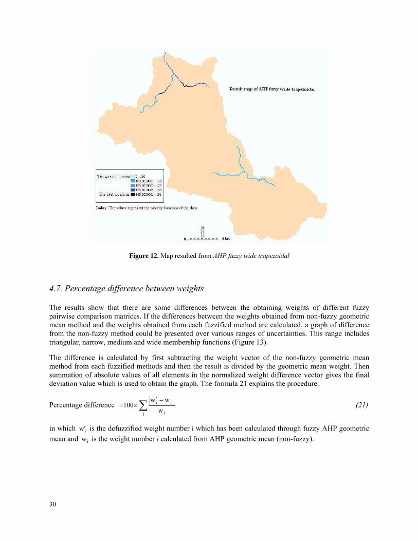
Figure 12. Map resulted from AHP fuzzy wide trapezoidal

4.7. Percentage difference between weights

The results show that there are some differences between the obtaining weights of different fuzzy pairwise comparison matrices. If the differences between the weights obtained from non-fuzzy geometric mean method and the weights obtained from each fuzzified method are calculated, a graph of difference from the non-fuzzy method could be presented over various ranges of uncertainties. This range includes triangular, narrow, medium and wide membership functions (Figure 13).

The difference is calculated by first subtracting the weight vector of the non-fuzzy geometric mean method from each fuzzified methods and then the result is divided by the geometric mean weight. Then summation of absolute values of all elements in the normalized weight difference vector gives the final deviation value which is used to obtain the graph. The formula 21 explains the procedure.

Percentage difference ∑ −′×=

i i

ii

www

100 (21)

in which is the defuzzified weight number i which has been calculated through fuzzy AHP geometric mean and is the weight number i calculated from AHP geometric mean (non-fuzzy).

iw′

iw

30

Figure 13. Percentage difference between the weights obtained from various levels of uncertainty in the fuzzy AHP

and Non-fuzzy AHP geometric mean.

4.8. Chi-Square ( χ ) test for Independence 2

The differences between the weights obtained from different methods led to use Chi-Square ( ) test to examine if there is any statistical relationship between the degree of uncertainty in fuzzification and the resulting map. All the obtained maps of different methods have five classes to show the priority of the locations. Each of the classes contains a number of pixels e.g. the resulted map of AHP geometric mean, contains 6 pixels in the class of priority one while the resulted map of fuzzy AHP by degree of uncertainty as triangular, contains 9 pixels in the class of priority one.

2χ

This difference raises the question: Is there any relationship between the degree of uncertainty and the number of pixels in each priority class of the maps. In fact the Chi-Square test was used to examine the question.

In Chi-Square test, the comparison between the maps is performed through comparing the number of pixels of river in each priority class at AHP and fuzzy AHP. Therefore for every uncertainty level there is a set of integer numbers which indicate the number of pixels of the river at every priority class. This set of numbers is compared, by Chi-Square test, with the corresponding set of AHP geometric mean.

The final judgment is performed by comparing the results of Chi-Square tests for all levels of uncertainty. This comparison is presented later after obtaining the results of all Chi-Square tests.

The Chi-Square test for examining the independence of two variables starts with a Null Hypothesis and an Alternative Hypothesis. The Null Hypothesis defined as there is no relationship between the variables. The Alternative Hypothesis indicates existence of some relationship between the variables (Dowdy et.al 2004). Here in this case the Null and Alternative Hypothesizes are defined as:

Null Hypothesis: H0 : The level of uncertainty has no effect on difference between the under testing map and the AHP geometric mean map.

Alternative Hypothesis: H1: The level of uncertainly can have some effects on difference between the under testing map and the AHP geometric mean map.

31

The Chi-Square statistic value is calculated by the following formula (Dowdy et.al 2004).

( )∑ −=χ

i i

2ii2

EEO (22)

in which is the observed value. Here in this case O is equal to the vector which indicates the number of pixels in each class of the examining map and

[ ]iOO =

[ ]iEE = is the expected value. Here E is equal to the vector which indicates the number of pixels in each priority class of the map related to AHP geometric mean method.

If the Null Hypothesis is correct, then EO = for each class and . So there is no relationship between the degree of uncertainty and difference between the maps. If the Alternative Hypothesis is correct then and the overall value of the test is large. If the obtained value is small then the Null Hypothesis cannot be rejected.

02 =χ

EO ≠ 2χ 2χ

For finding whether the obtained value is small or large, some items are considered. One of the items is Degree of Freedom (DF) which, in this case, is number of priority classes in each map i.e. 5, mines one; multiplied by number of examining maps i.e. 2, mines one; which finally is (5-1)×(2-1) =4. Significance level is another item of distribution which should be selected in the work. Traditionally researchers use level of 0.05 which is sometimes referred to as %5 significance level. In this work the same level has chosen as it provides a good reference point for final judgment.

2χ

2χ

From the table of distribution, the critical value can be determined when the significance level and the degree of freedom are known. In this case, with 4 degrees of freedom and 0.05 levels of significance, for the critical value the number of 9.488 is extracted from the distribution table. If the value obtained from the test is bigger than the critical value then the Null Hypothesis is rejected and if the value reported of the test is smaller than the critical value, the Null Hypothesis of no relationship between the variables cannot be rejected (Dowdy et.al 2004).

2χ 2χ

2χ 2χ 2χ2χ

2χ 2χ

The number of pixels in each priority class of the maps was required for performing the Chi-Square test and they are shown in Table 16.

Table 16. Number of pixels in each priority class of the maps with different levels of uncertainty.

priority 1 Number of pixels priority 2 priority 3 priority 4 priority 5 Total AHP geometric mean 6 38 69 152 13 278 AHP fuzzy triangular 9 38 68 152 11 278

AHP fuzzy narrow trapezoidal 11 38 66 152 11 278 AHP fuzzy medium trapezoidal 12 41 69 144 12 278

AHP fuzzy wide trapezoidal 13 42 61 151 11 278

For performing the test, a MATLAB code was written. After applying that for different level of uncertainty in fuzzy AHP, obtained Chi-Square values are mentioned in Table 17.

32

Table 17. The Chi-Square test values for different level of uncertainty in fuzzy AHP and AHP geometric mean.

Method AHP fuzzy triangular

AHP fuzzy narrow trapezoidal

AHP fuzzy medium trapezoidal

AHP fuzzy wide trapezoidal

Chi-Square test value 1.8222 4.6048 6.7348 9.8295

As it is shown in the Table 17, three of calculated values were smaller than 9.488 which is the critical value in the study i.e. AHP fuzzy triangular, AHP fuzzy narrow trapezoidal and AHP fuzzy medium trapezoidal .So for them, the observed values were similar to the expected values and the Null Hypothesis cannot be rejected. But in AHP fuzzy wide trapezoidal, the value is bigger than the critical value and it means that the Null Hypothesis must be rejected and the Alternative Hypothesis should be accepted. So test in this case shows that there is some relationship between degree of uncertainty and difference between the maps.

2χ2χ

2χ2χ

2χ

4.9. Comparison between maps

In order to analyze the optimum locations for the dam represented by maps with different degrees of uncertainty in AHP fuzzy, the result maps were compared with the maps obtained by AHP geometric mean which was the basic method of AHP for defuzzification. The comparison shows some differences in representing optimum locations for the dam in different maps. Moreover the comparisons between the AHP lambda max and AHP geometric mean maps also show some differences e.g., as is shown in Figure 14, in the AHP geometric mean map there are three pixels in the North part, shown with arrow, that show the best location for the dam while in AHP lambda max map these three pixels are not in the first priority class.

Figure 14. The comparison between the result maps of AHP geometric mean and AHP lambda max.

As it is stated in Table 16, the numbers of pixels in each priority class of the different maps are not the same so there could be some differences between the presented optimum locations of the dam in different maps. All the obtained maps of different methods are shown in previous part and it is easily possible to compare the presented locations in different priorities of the dam in more detail.

Focusing on a small section of the river, it is much easier to compare the resulted priority classes of all fuzzy AHP groups with AHP geometric mean. This small section is presented by a circle around it in

33

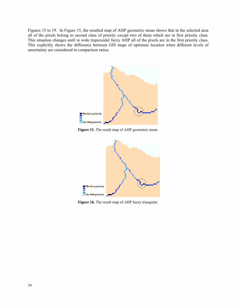
Figures 15 to 19. In Figure 15, the resulted map of AHP geometric mean shows that in the selected area all of the pixels belong to second class of priority except two of them which are in first priority class. This situation changes until in wide trapezoidal fuzzy AHP all of the pixels are in the first priority class. This explicitly shows the difference between GIS maps of optimum location when different levels of uncertainty are considered in comparison ratios.

Figure 15. The result map of AHP geometric mean.

Figure 16. The result map of AHP fuzzy triangular.

34

Figure 17. The result map of AHP fuzzy narrow trapezoidal.

Figure 18. The result map of AHP fuzzy medium trapezoidal.

Figure 19. The result map of AHP fuzzy wide trapezoidal.

35

5. Discussions and Conclusion

Having the resulting weights and final maps, the next step is to compare the results in a more conceptual manner. Earlier it was mentioned that Saaty (2008) is against fuzzifying the AHP. He concludes that fuzzification of the process does not give much different results. He also believes AHP is already a fuzzy process because most ratios for ranking are not absolute or crisp numbers. In fact, they are already fuzzy numbers and there is no theoretical proof that fuzzifying the comparison data leads to better results therefore it cannot be proved that fuzzifying AHP is a confident idea.

The above mentioned statement that AHP is already a fuzzy process is acceptable. The resulting weights and resulting maps of geometric mean and lambda max methods of the AHP are not the same. Comparing the weights obtained from lambda max and geometric mean methods, it can be seen that there is some difference between the two methods. There is no proof that which one is more acceptable or even closer to a reference vector of weights. In fact such a reference vector does not exist and the weights obtained from different methods are both equally acceptable. However it should be noticed that these differences between these two methods, and also between a numbers of other methods, are enough to conclude that there is some intrinsic uncertainty in the AHP which is in good agreement with Saaty’s considering AHP as an already fuzzy process.

Another issue which makes developing a pairwise comparison matrix in the AHP difficult is the fact that the comparison ratios are not exact numbers. It is known that AHP is developed to help decision-makers to evaluate the importance of some criteria or some alternatives. Mixing concepts of importance and exact numbers is difficult. The numbers 1,3,5,7 and 9 used in pairwise comparison matrix only indicate the importance of the corresponding factors. The way that the ratios in pairwise comparison matrix are defined is different from the meaning of numbers in algebra. For example if an arbitrary point A on the river is compared to point B , according to the economic criterion, by the number 3; it does not mean that economic benefits of point A is 3 times that of point B.What can be extracted from this number 3 is that point A has moderately higher economic benefits. Therefore any interpretation of the comparison ratios or even weights should be done considering this fact.

However till now little work, if any, has been done about the level of uncertainty. In most of the previous works AHP and fuzzy AHP have been compared when the uncertainty in comparison ratios was constant. But adding some more uncertainty to the comparison ratios makes the results much more different i.e. the higher level of uncertainty added to comparison ratios, results in more differences between AHP and fuzzy AHP. However in this work, by Chi-Square test, it has been shown that this difference grows slowly by increasing the level of uncertainty. In the first three levels of uncertainty, the effect of increasing the level of uncertainty on difference between the maps is insignificant although by increasing the level of uncertainty the Chi-Square test values are also growing. But the Chi-Square test values are still smaller than the critical value which indicate the result maps are almost similar to map resulted of AHP geometric mean. However in the AHP fuzzy wide trapezoidal, the Chi-Square test value is larger than the critical value so the influence of increasing the level of uncertainty is considerable and the result map of the method and the map resulted by AHP geometric mean are not the same.

2χ

2χ

The Chi-Square test was repeated for every different uncertainty levels of fuzzy AHP in the work. It should be mentioned that the result of each individual test is slightly dependent on the number of priority classes and how they are defined and also on the significance level chosen. However the overall conclusion remains intact and comparing the results it is concluded that the difference between the result maps of AHP geometric mean and the fuzzy AHP grows by increasing the uncertainty level.

36

References

Baban S. J. and Wan-Yusof K. 2003, Modelling Optimum Sites for Locating Reservoirs in Tropical Environments, Water Resources Management, Vol. 17, pp. 1–17.

Ballestero, M., 2003, Tárcoles River Basin Costa Rica. Background paper prepared for the World Bank research project “Integrated River Basin Management and the Principle of Managing Water Resources at the Lowest Appropriate Level – When and Why Does It (Not) Work in Practice?”, vi+114 p. Available at: http://siteresources.worldbank.org/INTSAREGTOPWATRES/Resources/CostaRica_Tarcoles_Background_FINAL.pdf

Boroushaki S. and Malczewski J. 2008, Implementing an extension of the analytical hierarchy process using ordered weighted averaging operators with fuzzy quantifiers in ArcGIS, Computers and Geosciences, Vol. 34, pp. 399–410

Brandt, S.A., 1999, Reservoir desiltation by means of hydraulic flushing: Sedimentological and Geomorphological Effects in Reservoirs and Downstream Reaches As Illustrated by the Cachí Reservoir and the Reventazón River, Costa Rica.Geographica Hafniensia, Vol. A8, pp. 231.

Buckley J.J. 1985, Fuzzy Hierarchical Analysis, Fuzzy sets and systems, Vol. 17, No. 3, pp. 233-247.

Chang D. Y. 1996, Application of the extent analysis method on fuzzy AHP, European Journal of Operational Research, Vol. 95, pp. 649-655.

Costa Rica, Tapanti National Park. 2008. Available at:

http://www.costarica.com/Places-To-See/Parks,-Reserves-and-Protected-Areas/Tapanti-National-Park/ [accessed 10 August 2008].

Dowdy Sh., Wearden S. and Chilko D., 2004, Statistics for Research. 3rd ed. New Jersey: John Wiley & Sons, Inc. Eastman J. R. 2003, IDRISI Kilimanjaro Guide to GIS and Image Processing, Idrisi Source Code. ESRI 2008, Arc GIS Desktop Help 9.2. [Online]. Avalable at: http://webhelp.esri.com/arcgisdesktop/9.2/index.cfm?TopicName=welcome [accessed 10 August 2008].

Gismalla Y.A. and Bruen M. 1996, Use of a GIS in reconnaissance studies for small-scale hydropower development in a developing country: a case study from Tanzania, Application of Geographic Information System in Hydrology and Water Resources Management, Vol. 235.

Han W.J. and Tsay W.D. 1998, Formulation of Quality Strategy Using Analytic Hierarchy Process, Twenty Seven Annual Meeting of the Western Decision Science Institute, University of Northern Colorado, USA, pp. 580–583.

Malczewski J. 1999, GIS and Multicriteria Desision Analysis, New York: John Willey and Sons, Inc.

Malczewski J. 2006, GIS-based multicriteria decision analysis: a survey of the literature, International Journal of Geographical Information Science, Vol. 20, No. 7, pp. 703–726.

Saaty L.T. (1980), The Analytic Hierarchy Process, New York, McGraw-Hill International.

37

Saaty L.T. 1990, How to make a decision: The Analytic Hierarchy Process, European Journal of Operational Research, Vol. 48, pp. 9-26.

Saaty L.T. 2006, Rank from comparisons and from ratings in the analytic hierarchy/network processes, European Journal of Operational Research, Vol. 168, pp. 557-570.

Saaty T.L. and Tran L.T. 2007, On the invalidity of fuzzifying numerical judgments in the Analytic Hierarchy Process, Mathematical and Computer Modelling, Vol. 46, pp. 962–975.

Saaty T.L. and Tran L.T. 2008, Fuzzy Judgments and Fuzzy Sets, Unpublished report. Saaty T.L. 2008, There is no Mathematical Validity for Using Fuzzy Number Crunching in the Analytic Hierarchy Process, Unpublished report. Saborio, J., no year, Mapeo digital del potencial de erosion, cuenca Río Reventazón, Costa Rica, Unpuplished report, Instituto Costarricence de Electricidad.

Sánchez-Azofeifa G.A., Daily G.C., Pfaff A.S.P. and Busch Ch. 2003, Integrity and isolation of Costa Ricas national parks and biological reseves:examining the dynamics of land-cover change, Biological Conservation, Vol. 109, pp. 123-135.

Vahrson, W.-G., 1992: Tropische Starkregen und ihre Verteilung - das Beispiel des Einzugsgebietes des Río Reventazón, Costa Rica (Spatial distribution of heavy rainfalls in the tropics - the example of the Río Reventazón catchment, Costa Rica). Die Erde, Vol. 123, No.1, pp. 1-15. Yang Ch.Ch. and Chen B.Sh. 2004, Key Quality Performance Evaluation Using Fuzzy AHP, Journal of the Chinese Institute of Industrial Engineers, Vol. 21, No. 6, pp. 543-550.

Zimmermann H.J., 1934. Fuzzy Set Theory—and Its Applications. 3rd ed. Boston/Dordrecht/London: Kluwer Academic Publishers.

38

Appendix A

The Script for Making the Water discharge:

theView = av.GetActiveDoc

thegTheme = theView.getactivethemes.get(0)

agrid = thegtheme.getgrid

theGrid = theView.FindTheme("flow direction").GetGrid

thePrj = theView.GetProjection

runoff = agrid * 1.asgrid

flowAccGrid = thegrid.FlowAccumulation(runoff)

theGTheme = Gtheme.Make(flowaccgrid)

if(flowaccgrid.HasError)then

return(NIL)

end

theView.addTheme(theGtheme)

39

Appendix B: The landuse of study area, factor and constraint maps of the project.

Figure 20. Different landuse of study area.

Figure 21. Factor map of Undulation.

40

Figure 22. Factor map of Road.

Figure 23. Factor map of City.

41

Figure 24. Factor map of Road Water flow.

Figure 25. Factor map of Hydraulic head.

42

Figure 26. Factor map of Agriculture.

Figure 27. Factor map of Forest.

43

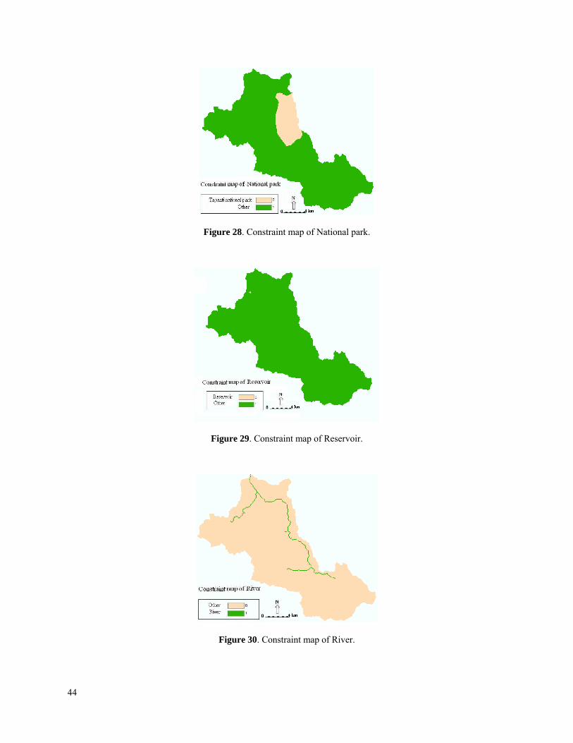
Figure 28. Constraint map of National park.

Figure 29. Constraint map of Reservoir.

Figure 30. Constraint map of River.

44

Appendix C: Fuzzy weights for fuzzy membership functions.

Fuzzy weights for fuzzy triangular membership functions.

0 0.1 0.2 0.3 0.4 0.5 0.6 0.7 0.8 0.9 10

0.5

1

1.5Weight1 for aTriangular membership function

Figure 31. Weight 1 of the fuzzy AHP trangular: (0.0183, 0.0290, 0.0290, 0.0500)

0 0.1 0.2 0.3 0.4 0.5 0.6 0.7 0.8 0.9 10

0.5

1

1.5Weight2 for aTriangular membership function

Figure 32. Weight 2 of the fuzzy AHP trangular: (0.0294, 0.0495, 0.0495, 0.0897)

45

0 0.1 0.2 0.3 0.4 0.5 0.6 0.7 0.8 0.9 10

0.5

1

1.5Weight3 for aTriangular membership function

Figure 33. Weight 3 of the fuzzy AHP trangular: (0.0463, 0.0804, 0.0804, 0.1520)

0 0.1 0.2 0.3 0.4 0.5 0.6 0.7 0.8 0.9 10

0.5

1

1.5Weight4 for aTriangular membership function

Figure 34. Weight 4 of the fuzzy AHP trangular: (0.0602, 0.1128, 0.1128, 0.2204)

0 0.1 0.2 0.3 0.4 0.5 0.6 0.7 0.8 0.9 10

0.5

1

1.5Weight5 for aTriangular membership function

Figure 35. Weight 5 of the fuzzy AHP trangular: (0.1029, 0.1864, 0.1864, 0.3616)

46

0 0.1 0.2 0.3 0.4 0.5 0.6 0.7 0.8 0.9 10

0.5

1

1.5Weight6 for aTriangular membership function

Figure 36. Weight 6 of the fuzzy AHP trangular: (0.1192, 0.2293, 0.2293, 0.4285)

0 0.1 0.2 0.3 0.4 0.5 0.6 0.7 0.8 0.9 10

0.5

1

1.5Weight7 for aTriangular membership function

Figure 37. Weight 7 of the fuzzy AHP trangular: (0.1647, 0.3126, 0.3126, 0.5465)

Fuzzy weights for fuzzy narrow trapezoidal membership fanctions.

0 0.1 0.2 0.3 0.4 0.5 0.6 0.7 0.8 0.9 10

0.5

1

1.5Weight1 for aNarrow Trapezoidal membership function

Figure 38. Weight 1 of the AHP fuzzy narrow trapezoidal: (0.0162, 0.0230, 0.0373, 0.0593)

47

0 0.1 0.2 0.3 0.4 0.5 0.6 0.7 0.8 0.9 10

0.5

1

1.5Weight2 for aNarrow Trapezoidal membership function

Figure 39. Weight 2 of the AHP fuzzy narrow trapezoidal: (0.0256, 0.0381, 0.0653, 0.1079)

0 0.1 0.2 0.3 0.4 0.5 0.6 0.7 0.8 0.9 10

0.5

1

1.5Weight3 for aNarrow Trapezoidal membership function

Figure 40. Weight 3 of the AHP fuzzy narrow trapezoidal: (0.0399, 0.0611, 0.1080, 0.1864)

0 0.1 0.2 0.3 0.4 0.5 0.6 0.7 0.8 0.9 10

0.5

1

1.5Weight4 for aNarrow Trapezoidal membership function

Figure 41. Weight 4 of the AHP fuzzy narrow trapezoidal: (0.0501, 0.0831, 0.1545, 0.2719)

48

0 0.1 0.2 0.3 0.4 0.5 0.6 0.7 0.8 0.9 10

0.5

1

1.5Weight5 for aNarrow Trapezoidal membership function

Figure 42. Weight 5 of the AHP fuzzy narrow trapezoidal: (0.0872, 0.1391, 0.2535, 0.4487)

0 0.1 0.2 0.3 0.4 0.5 0.6 0.7 0.8 0.9 10

0.5

1

1.5Weight6 for aNarrow Trapezoidal membership function

Figure 43. Weight 6 of the AHP fuzzy narrow trapezoidal: (0.0968, 0.1687, 0.3098, 0.5164)

0 0.1 0.2 0.3 0.4 0.5 0.6 0.7 0.8 0.9 10

0.5

1

1.5Weight7 for aNarrow Trapezoidal membership function

Figure 44. Weight 7 of the AHP fuzzy narrow trapezoidal: (0.1333, 0.2327, 0.4124, 0.6364)

49

Fuzzy weights for fuzzy medium trapezoidal membership fanctions.

0 0.1 0.2 0.3 0.4 0.5 0.6 0.7 0.8 0.9 10

0.5

1

1.5Weight1 for aMedium Trapezoidal membership function

Figure 45. Weight 1 of the AHP fuzzy medium trapezoidal: (0.0142, 0.0205, 0.0429, 0.0722)

0 0.1 0.2 0.3 0.4 0.5 0.6 0.7 0.8 0.9 10

0.5

1

1.5Weight2 for aMedium Trapezoidal membership function

Figure 46. Weight 2 of the AHP fuzzy medium trapezoidal: (0.0219, 0.0335, 0.0760, 0.1337)

0 0.1 0.2 0.3 0.4 0.5 0.6 0.7 0.8 0.9 10

0.5

1

1.5Weight3 for aMedium Trapezoidal membership function

Figure 47. Weight 3 of the AHP fuzzy medium trapezoidal: (0.0339, 0.0533, 0.1271, 0.2386)

50

0 0.1 0.2 0.3 0.4 0.5 0.6 0.7 0.8 0.9 10

0.5

1

1.5Weight4 for aMedium Trapezoidal membership function

Figure 48. Weight 4 of the AHP fuzzy medium trapezoidal: (0.0403, 0.0711, 0.1831, 0.3499)

0 0.1 0.2 0.3 0.4 0.5 0.6 0.7 0.8 0.9 10

0.5

1

1.5Weight5 for aMedium Trapezoidal membership function

Figure 49. Weight 5 of the AHP fuzzy medium trapezoidal: (0.0724, 0.1200, 0.3001, 0.5874)

0 0.1 0.2 0.3 0.4 0.5 0.6 0.7 0.8 0.9 10

0.5

1

1.5Weight6 for aMedium Trapezoidal membership function

Figure 50. Weight 6 of the AHP fuzzy medium trapezoidal: (0.0747, 0.1429, 0.3624, 0.6448)

51

0 0.1 0.2 0.3 0.4 0.5 0.6 0.7 0.8 0.9 10

0.5

1

1.5Weight7 for aMedium Trapezoidal membership function

Figure 51. Weight 7 of the AHP fuzzy medium trapezoidal: (0.1022, 0.1976, 0.4737, 0.7548)

Fuzzy weights for fuzzy wide trapezoidal membership fanctions.

0 0.1 0.2 0.3 0.4 0.5 0.6 0.7 0.8 0.9 10

0.5

1

1.5Weight1 for aWide Trapezoidal membership function

Figure 52. Weight 1 of the AHP fuzzy wide trapezoidal :( 0.0142, 0.0152, 0.0651, 0.0722)

0 0.1 0.2 0.3 0.4 0.5 0.6 0.7 0.8 0.9 10

0.5

1

1.5Weight2 for aWide Trapezoidal membership function

Figure 53. Weight 2 of the AHP fuzzy wide trapezoidal: (0.0219, 0.0238, 0.1195, 0.1337)

52

0 0.1 0.2 0.3 0.4 0.5 0.6 0.7 0.8 0.9 10

0.5

1

1.5Weight3 for aWide Trapezoidal membership function

Figure 54. Weight 3 of the AHP fuzzy wide trapezoidal: (0.0339, 0.0369, 0.2094, 0.2386)

0 0.1 0.2 0.3 0.4 0.5 0.6 0.7 0.8 0.9 10

0.5

1

1.5Weight4 for aWide Trapezoidal membership function

Figure 55. Weight 4 of the AHP fuzzy wide trapezoidal: (0.0403, 0.0452, 0.3062, 0.3499)

0 0.1 0.2 0.3 0.4 0.5 0.6 0.7 0.8 0.9 10

0.5

1

1.5Weight5 for aWide Trapezoidal membership function

Figure 56. Weight 5 of the AHP fuzzy wide trapezoidal: (0.0724, 0.0797, 0.5087, 0.5874)

53

0 0.1 0.2 0.3 0.4 0.5 0.6 0.7 0.8 0.9 10

0.5

1

1.5Weight6 for aWide Trapezoidal membership function

Figure 57. Weight 6 of the AHP fuzzy wide trapezoidal: (0.0747, 0.0858, 0.5735, 0.6448)

0 0.1 0.2 0.3 0.4 0.5 0.6 0.7 0.8 0.9 10

0.5

1

1.5Weight7 for aWide Trapezoidal membership function

Figure 58. Weight 7 of the AHP fuzzy wide trapezoidal: (0.1022, 0.1178, 0.6908, 0.7548)

54