FISCAL SUSTAINABILITY CONVERGENCE:

HOW THE CRISIS CAUGHT ‘OLD’ EUROPE UNPREPARED

Ivaylo A. Nikolov*

Bulgarian National Bank

This version: 15 January 2010

Abstract

Previous studies disagree on the fiscal sustainability of ‘old’ Europe but the topic has regained importance during the recent economic crisis. This paper proposes a way to assess fiscal sustainability convergence over time, addressing two sequential research questions: has long-run fiscal sustainability been achieved, and if so has more sustainability been derived from the European fiscal rules. The method can also be used to track any future progress towards sustainability. The empirical results provide robust evidence against fiscal sustainability. Neither Maastricht, nor the Stability and Growth Pact, nor the actual advent of the Euro seem to have mattered in streamlining any efforts to run public finances in keeping with the intertemporal budget constraint. The post-2007 crisis has caught ‘old’ Europe fiscally unprepared, policy changes were required earlier, and the impending fiscal consolidations will need to be faster and more ambitious than currently considered.

Keywords: Fiscal Sustainability; Convergence; Stability and Growth Pact; European Union.

JEL Classification: C22; E62; H30.

Correspondence to: Ivaylo A. Nikolov, Bulgarian National Bank, 1 Knyaz Alexander І sq., Sofia 1000, Bulgaria. Tel: +359 (2) 9145 1937; Fax: +359 (2) 9145 1795; E-mail: Nikolov.I@bnbank.org

*I am indebted to Andrey Vassilev, Christopher J. Green, Dimitar Vasilev and Slavi T. Slavov for constructive ideas, comments and suggestions on an earlier version of this paper. The usual disclaimer applies.

1

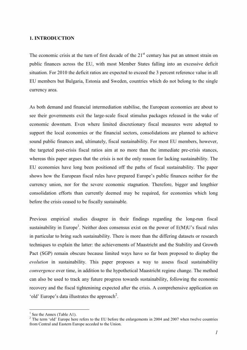
1. INTRODUCTION

The economic crisis at the turn of first decade of the 21st century has put an utmost strain on

public finances across the EU, with most Member States falling into an excessive deficit

situation. For 2010 the deficit ratios are expected to exceed the 3 percent reference value in all

EU members but Bulgaria, Estonia and Sweden, countries which do not belong to the single

currency area.

As both demand and financial intermediation stabilise, the European economies are about to

see their governments exit the large-scale fiscal stimulus packages released in the wake of

economic downturn. Even where limited discretionary fiscal measures were adopted to

support the local economies or the financial sectors, consolidations are planned to achieve

sound public finances and, ultimately, fiscal sustainability. For most EU members, however,

the targeted post-crisis fiscal ratios aim at no more than the immediate pre-crisis stances,

whereas this paper argues that the crisis is not the only reason for lacking sustainability. The

EU economies have long been positioned off the paths of fiscal sustainability. The paper

shows how the European fiscal rules have prepared Europe’s public finances neither for the

currency union, nor for the severe economic stagnation. Therefore, bigger and lengthier

consolidation efforts than currently deemed may be required, for economies which long

before the crisis ceased to be fiscally sustainable.

Previous empirical studies disagree in their findings regarding the long-run fiscal

sustainability in Europe1. Neither does consensus exist on the power of E(M)U’s fiscal rules

in particular to bring such sustainability. There is more than the differing datasets or research

techniques to explain the latter: the achievements of Maastricht and the Stability and Growth

Pact (SGP) remain obscure because limited ways have so far been proposed to display the

evolution in sustainability. This paper proposes a way to assess fiscal sustainability

convergence over time, in addition to the hypothetical Maastricht regime change. The method

can also be used to track any future progress towards sustainability, following the economic

recovery and the fiscal tightenining expected after the crisis. A comprehensive application on

‘old’ Europe’s data illustrates the approach2.

1 See the Annex (Table A1). 2 The term ‘old’ Europe here refers to the EU before the enlargements in 2004 and 2007 when twelve countries from Central and Eastern Europe acceded to the Union.

2

At first sight the analysis of historical data should reveal whether or not EU members are in

fact compliant with the intertemporal budget constraint (IBC): and then Maastricht/SGP

might automatically be (dis)credited for the results. This seems to have been the research

route followed so far in the European fiscal sustainability literature. Using this approach

however, it could be argued that the exact contribution of the E(M)U to fiscal sustainability

may never be extracted unless the stages in any convergence towards sustainability are

identified.

The rules of the E(M)U seek to impose fiscal discipline on the road to and then within the

monetary union and, as the next section shows, the 1990s do point to significant fiscal

adjustments in some countries. Whereas the ‘backward-looking’ statistical analysis is not

directly compatible with those rules, it can nonetheless test the hypothesis if fiscal

sustainability has been achieved; hence whether the Maastricht Treaty and SGP definitions

correspond to the notion of long-run fiscal sustainability. Moreover, the statistical tests can

reveal when historical sustainability of fiscal policies has been attained.

How sustainability is achieved or changes over time, are issues almost never discussed in the

empirical literature. Some studies note that more complex dynamics with particular instances

of structural breaks exist (e.g. Tanner and Liu, 1994, Liu and Tanner, 1995, Quintos, 1995,

Arghyrou and Luintel, 2007, or for all the EU15 countries Afonso, 2005). De Bandt and

Mongelli (2000) use ‘convergence’ in a different context to measure the correlation between

key fiscal variables and also the existing pairwise cointegration among country and group

(European) averages. Blot and Serranito (2006) analyse convergence in certain EMU fiscal

policy indicators but not in the sustainability of fiscal policy in the IBC sense.

A notable contribution is Prazmowski’s (2005) study of the Dominican Republic based on

recursive cointegration but his approach differs in that he uses the Kalman filter and also does

not validate the method and its results across more (or European) countries. Before that

Hatemi-J (2002b) also applies the Kalman filter on Swedish quarterly data from 1963 till

2000 to estimate a time varying coefficient model. While my research agenda also involves

the recursive estimation of a slope parameter, I draw on a simple and transparent dynamic

OLS cointegration analysis and a dataset covering almost the entire ‘old’ Europe. That is

3

complemented by an explicit treatment of the Maastricht shift, further highlighting the

performance in the 1990s and beyond, up until the current economic crisis.

In summary, this paper addresses the two sequential research questions: have the EU14

countries achieved long-run fiscal sustainability over the period in question, and if so have

they become more sustainable due to Maastricht and the SGP3? The empirical applications

examine the hypothetical gradual convergence towards or away from fiscal sustainability, as

well as the particular effect from the Maastricht Treaty. The narrative goes as follows. The

next section reviews the fiscal experience of Western Europe, based on the two Maastricht

fiscal rules, in the run-up to the EMU and in the first years of its existence. The research

methods and strategy are outlined then, followed by the section with the data and empirical

findings. A brief summary of results and policy implications concludes the paper. Annex

Table A1 provides a detailed summary of empirical works on Europe belonging to the

econometric ‘backward looking’ approach to fiscal sustainability.

2. FISCAL POLICY BEFORE AND AFTER THE EURO

This section presents the main fiscal aggregates from the EU comprising the members before

the two enlargement waves in 2004 and 2007. This provides an intuitive view of the

hypothesis for convergence towards sustainability since the Maastricht Treaty was signed in

1992 and before the onset of crisis, as a background for the more formal analysis later.

2.1. General government fiscal balances

Article 104 of the Maastricht Treaty declares that EU member states should avoid excessive

deficits. Article 1 of the Protocol on the excessive deficit procedure (EDP) to the Treaty

stipulates that the reference value is 3 percent for the ratio of planned or actual government

deficit to GDP at market prices. The SGP in 1997 re-stated that limit, emphasising that within

it ‘dealing with normal cyclical fluctuations’, hence also the operation of automatic fiscal

stabilisers, is still possible. The enforcement mechanism is stronger for EMU members than

for non-Euro member countries. When the latter have excessive deficits, recommendations are

3 EU14 denotes ‘old’ Europe without Luxembourg. Historical data for that country are scarcer. Omitting it would hardly alter the overall conclusions about fiscal sustainability in Europe, as the size of Luxembourg’s economy is relatively negligible (in 2008 its GDP at market prices was 0.3 percent of the total of ‘old’ Europe).

4

made by the Council. These recommendations according to Article 104(7) are not made

public unless no effective measures are taken by the member country. However, the notices

under Article 104(9) and the sanctions under Article 104(11) are not applied to non-Euro

members (EC, 2006, p. 40, Box I.1).

Figures 1 illustrates the dynamics of general government budget balances and gross debt, both

as percent of GDP, in the pre-2004-enlargement EU.

[Figure 1 about here]

Following the deterioration in the overall budget stance since the mid-1970s (arguably due to

the oil shocks in that decade: see Fatás and Mihov, 2003, p. 116), Figure 1 reveals the fiscal

turbulences starting from the early 1990s. Concerning the budget balances, individual country

experiences differ substantially, yet a common pattern of fiscal adjustment is observed with

the best fiscal positions achieved around the turn of the century in nearly all countries.

It is also evident that the three non-EMU members performed rather similarly to the rest. One

conjecture would be that all countries have been well integrated through common trade, cross-

border investments and perhaps synchronisation of the business cycles. Hence national

budgets have reflected that. Such a surmise deserves a separate study and may not be equally

valid for each country, but the experiences of Denmark, Sweden and the United Kingdom

indirectly challenge any straightforward explanation that it was just the signing of the

Maastricht Treaty that set off the improvement in fiscal sustainability throughout the nineties.

Yet the Maastricht convergence criteria must have mattered for countries eager to adopt the

single currency. Indirect evidence for that is the widespread deterioration in fiscal balances

right after 1999. It may intuitively be implied that, having joined the EMU, countries found

the SGP fiscal burdens less binding. For some such as Germany the time had come for

structural reforms while for others such as Portugal the Euro exposed the lack of

competitiveness of the economy. In many cases the result was higher deficits or at least looser

fiscal policies.

5

2.2. General government debt

The second fiscal provision stemming from Maastricht is that the gross general government

consolidated debt at nominal value should not exceed 60 percent of GDP at market prices.

That criterion is taken into account when reviewing the performance of candidates for full-

EMU membership. In their ‘convergence programmes’ debt data and projected debt paths are

reported, whereas the current EMU members report those in their ‘stability programmes’

(Council Regulation 1466/97). Thus compliance is monitored for all EU members under the

surveillance based on the Excessive Deficit Procedure, however in practice no binding

disciplinary action can be taken if the debt limits are breached by existing EMU members or

by the two ‘old’ members with the ‘opt-out’ clause (Denmark and the United Kingdom).

Even in the run-up to the third stage of the EMU, the Maastricht debt criterion was viewed

more flexibly and considered with greater scope for discretion. Against the very high

debt/GDP ratios for some European countries, the Treaty allowed for exceeding the reference

value in cases when ‘the ratio is sufficiently diminishing and approaching the reference value

at a satisfactory pace’ (Article 104).

It should therefore not necessarily be expected for the debt/GDP ratios to have declined

before 1999 or afterwards, although convergence towards the 60 percent value is likely. And

that is indeed the overall message of Figure 1 which shows debt defined according to the

Maastricht definition.

It can be seen that the years just before the Euro witnessed a dominant decline in the general

government debt/GDP ratio, although the Euro area was formed in 1999 with an overall ratio

still above the 60 percent threshold. Debt/GDP for the whole Euro area remained higher than

in the EU14. Certainly individual countries differ: the United Kingdom had lower

indebtedness while some Euro area countries (notably Italy, Belgium and Greece) exhibited

very high debt/GDP ratios. Ireland managed to reduce its Maastricht debt from over 90

percent of GDP in 1990 to 54 percent of GDP in 1998; after joining the EMU, debt reduction

there continued to reach as low as 25 percent of GDP in 2006.

Declining debt in the late 1990s generally reflects the improvement in budget balances. That

may be implied for most individual countries, though with exceptions such as Greece, with a

6

continually high debt, and Austria, where budget deficits shrank while debt as a share of GDP

did not change significantly in the years just before the Euro. Germany and France similarly

did not succeed in reducing debt despite some budget consolidation right in the run-up to the

single currency. Although high, the debt/GDP ratio of Belgium from Figure 1 shows a

declining trend throughout most of the period.

3. THE FISCAL SUSTAINABILITY CONVERGENCE FRAMEWORK

3.1. Between Maastricht and the long-run fiscal sustainability criteria

The overall budget balances and general government debt data from Europe present varied

degrees of compliance with the fiscal criteria from Maastricht and the SGP, both before and

after the countries adopted the Euro. A tentative suggestion is therefore that despite efforts to

ensure the sustainable public finances required (in a Ricardian sense4) in a monetary union,

evidence has been mixed.

Yet even for countries with seemingly successful short-term adjustments an open question

remains: have fiscal outcomes even within the Maastricht bounds contributed to long-run

fiscal sustainability? From that perspective, the analysis of fiscal sustainability in ‘old’

Europe should resort to more formal methods.

Fiscal sustainability is associated with the ability of a government to bear the costs of existing

debt, that is to stay solvent, and with any constraints over time needed to keep or restore that

solvency. The current fiscal stance is deemed sustainable when it does not lead to bankruptcy

in the future, even if solvency is not an imminent issue. More technically, fiscal sustainability

is present when the current government debt equals the present value of the future budget

surpluses or their excess over deficits: and historical data can be analysed for compliance with

such an intertemporal constraint.

4 See McCallum (1984).

7

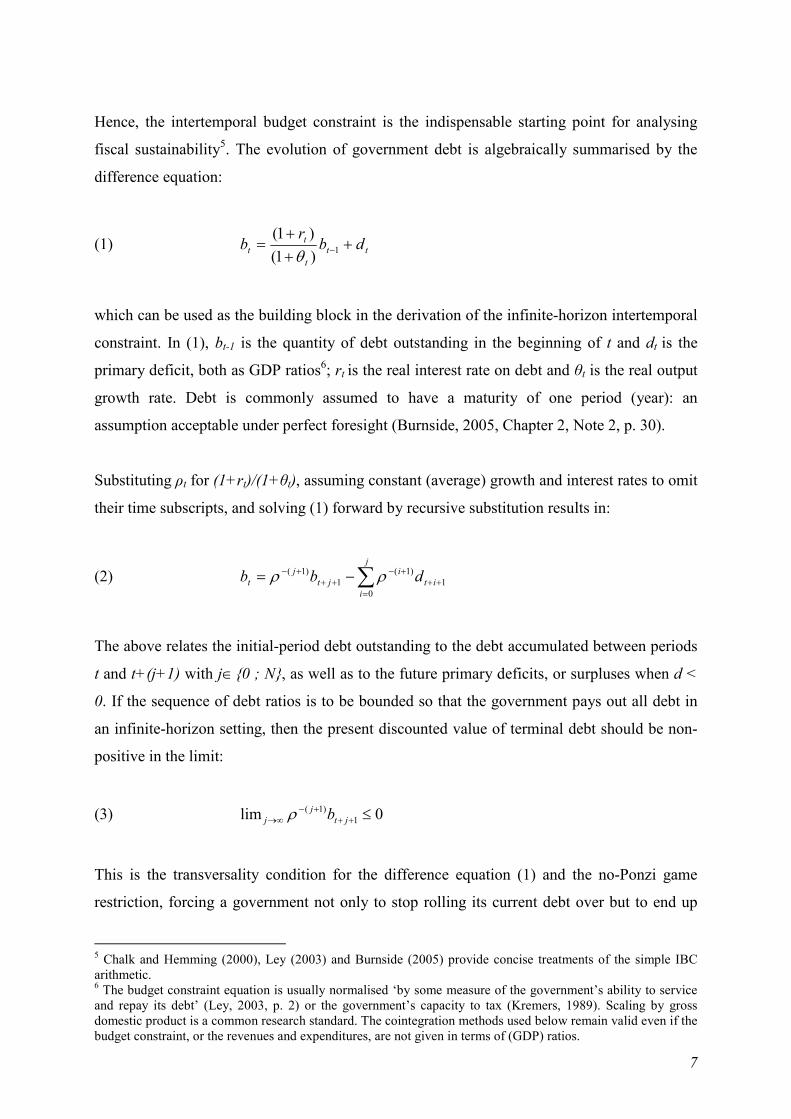
Hence, the intertemporal budget constraint is the indispensable starting point for analysing

fiscal sustainability5. The evolution of government debt is algebraically summarised by the

difference equation:

(1) ttt

tt db

rb +

++

= −1)1()1(

θ

which can be used as the building block in the derivation of the infinite-horizon intertemporal

constraint. In (1), bt-1 is the quantity of debt outstanding in the beginning of t and dt is the

primary deficit, both as GDP ratios6; rt is the real interest rate on debt and θt is the real output

growth rate. Debt is commonly assumed to have a maturity of one period (year): an

assumption acceptable under perfect foresight (Burnside, 2005, Chapter 2, Note 2, p. 30).

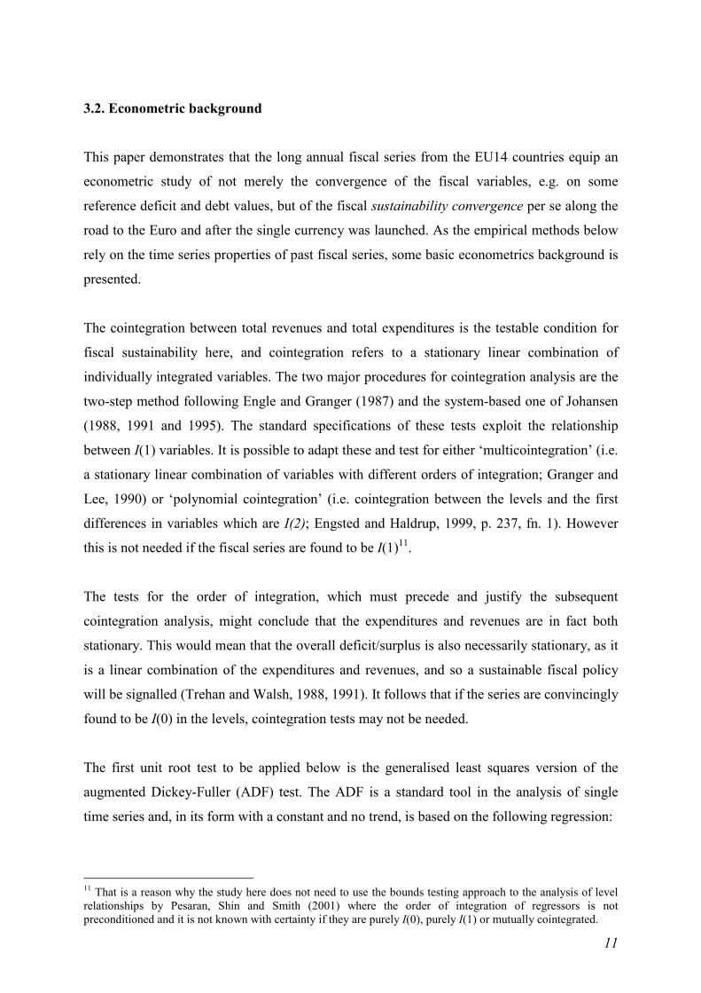
Substituting ρt for (1+rt)/(1+θt), assuming constant (average) growth and interest rates to omit

their time subscripts, and solving (1) forward by recursive substitution results in:

(2) ∑=

+++−

+++− −=

j

iit

ijt

jt dbb

01

)1(1

)1( ρρ

The above relates the initial-period debt outstanding to the debt accumulated between periods

t and t+(j+1) with j∈{0 ; N}, as well as to the future primary deficits, or surpluses when d <

0. If the sequence of debt ratios is to be bounded so that the government pays out all debt in

an infinite-horizon setting, then the present discounted value of terminal debt should be non-

positive in the limit:

(3) 0lim 1)1( ≤++

+−∞→ jt

jj bρ

This is the transversality condition for the difference equation (1) and the no-Ponzi game

restriction, forcing a government not only to stop rolling its current debt over but to end up

5 Chalk and Hemming (2000), Ley (2003) and Burnside (2005) provide concise treatments of the simple IBC arithmetic. 6 The budget constraint equation is usually normalised ‘by some measure of the government’s ability to service and repay its debt’ (Ley, 2003, p. 2) or the government’s capacity to tax (Kremers, 1989). Scaling by gross domestic product is a common research standard. The cointegration methods used below remain valid even if the budget constraint, or the revenues and expenditures, are not given in terms of (GDP) ratios.

8

without any outstanding debt. Provided that (3) holds as equality, (2) turns into the

intertemporal constraint of the form7:

(4) ∑∞

=++

+−−=0

1)1(

iit

it db ρ

If taken as an accounting identity, the constraint of (4) may be considered to hold permanently

or, more precisely, ex post (Blanchard, 1990, p. 13). The latter consideration is fundamental

for the research approaches to fiscal sustainability, although interpretations vary. One may

focus on the specific changes required ex ante in order to satisfy the IBC, and may also

‘augment’ them by further collateral constraints (like the fiscal rule limiting the debt/GDP

ratio). Another approach is to test empirically the past fiscal performance: to see if the IBC

has actually been observed, and if not whether some fiscal adjustments are inevitable in the

future. Broadly speaking, those two attitudes have inspired two distinct strands of the fiscal

sustainability literature.

This paper belongs to the ‘backward-looking’ strand which econometrically examines the past

fiscal stance. Although the IBC should always hold ex post, for shorter time series there may

be deviations from it. Correspondingly, the theory of fiscal sustainability has distilled

empirically testable conditions. If these conditions are met by the past data, the government

will be able to pay out its debt, hence it is fiscally sustainable. Such methods assume that the

fiscal policies will remain unchanged and the data from the past are regarded as representative

of the long-run infinite future. When the sequence of fiscal variables from the past, if

supposed to be continued into the future, suggests to be satisfying an intertemporal present-

value constraint, the fiscal position is regarded as sustainable. Thus in the context of Europe,

this paper discusses whether fiscal policies, if looking back at historical data, satisfied the IBC

- before the advent of the current crisis - without any need for future changes in policy.

Hamilton and Flavin’s (1986) pioneering work yields the stationarity of government debt as

the condition for fiscal sustainability. Later papers have developed alternative models based

on stationarity conditions. Thus Trehan and Walsh (1988) proved that stationarity of the first

difference of the stock of debt is sufficient for fiscal sustainability, as is the stationarity of the

7 A negative sign in (3) implies that individuals can be left on the borrowing side, enabling them to run ‘rational Ponzi schemes’ against the government (see O’Connell and Zeldes, 1988, p. 437).

9

overall deficit. Others based their sustainability conditions on cointegration theory. In Haug

(1991) fiscal sustainability requires that debt and primary deficit be cointegrated.

Cointegration between revenues and total expenditures, along with unitary cointegrating

parameter on the latter, suffice according to Hakkio and Rush (1991a) and the ‘strong’

sustainability condition defined by Quintos (1995).

Hakkio and Rush (1991a) start with a budget equation of the form8:

(5) jtjtjti

itjtt BGTB +−

+∞→

∞

+=

−+ +−= ∑ 1

1

1 )(lim)()( ρρ

where the B is debt and T and G, respectively, stand for total revenue and expenditures. The

interest rate is allowed to vary and ρ is a discount factor. IBC implies that the limit term in (5)

equals zero.

Hakkio and Rush (1991a) explore the stochastic properties of the processes of primary

balance components that would condition the expected value of the limiting discounted debt

to be zero9. They first assume that the interest rate is stationary around an unconditional mean

r. Then a new relation is constructed:

(6) Et = Gt + (rt – r)Bt-1

which represents government expenditures plus that part of interest payments on previous-

period debt that corresponds to the deviation of current interest rate from its mean value. Total

government expenditures (denoted GGt = Gt + rtBt-1) are shown to form the following

intertemporal constraint:

(7) jtj

jjjtjt

jtt BrETrTGG +

+−∞

=∞→++

−− ++∆−∆++= ∑ )1(

0

)1( )1(lim)()1(

8 The original notation is adapted here. 9 Hakkio and Rush (1991a, p. 431) note a generic shortcoming of the statistical tests approach to fiscal sustainability analysis: ‘… since we often know things about the future that are not included in the historical record … [and] … this drawback exists in all work that focuses on the time series behavior of data.’

10

Ruling out Ponzi-type attempts to issue new debt in order to finance deficits, and further

imposing a repayment of all government debt, will in (7) be satisfied if the limit term equals

zero. Hakkio and Rush (1991a) prove that the IBC holds when total expenditures and

revenues are cointegrated and the estimate of the coefficient on total expenditures (when

regressing revenues on expenditures) equals 1.

Quintos (1995) has left the fiscal sustainability literature with an option to permit a more

relaxed definition: revenues and total expenditures need not be cointegrated as long as the

independent variable’s parameter estimate in the bivariate regression lies between 0 and 1. It

is admitted however that although the deficit process may be ‘integrated or even mildly

explosive and the deficit will still be sustainable’ that ‘has serious policy implications because

a government that continues to spend more than it earns has a high risk of default’ (ibid., p.

410). The ‘weak’ sustainability condition may potentially strain an economy with a rising

debt; therefore it will be safer if the data support the ‘stronger’ sustainability case.

The above testable conditions nest a special case when the IBC is satisfied: if the total

expenditures and revenues series are individually I(0).

A further argument for resorting to the cointegration analysis of fiscal sustainability stems

from Ahmed and Rogers (1995). They show that, under some very general conditions

cointegration between total revenue and total expenditures is necessary and sufficient for

sustainability even in a stochastic environment. This paper extends that body of literature

where the revenue-expenditure cointegration criterion is applied. Leaving aside the ‘weak’

condition by Quintos (1995) commented below, total revenues and expenditures, if not

stationary in their levels, should be cointegrated with a vector (1, -1) to claim fiscal

sustainability in the EU14 sample10.

10 More recently Bohn (2007) challenged the necessity to have first-difference stationary debt or cointegration between expenditures and revenues; although he still allows these conditions, if not rejected, to be sufficient for fiscal sustainability. But for practical purposes the cointegration analysis remains justifiable because Bohn’s (2007) proposition that sustainability is in place when debt is integrated of any higher order is equivalent to allowing at least quadratic debt growth. The latter will hardly be welcome by potential government-bond holders, hence fiscal sustainability will be at risk. Furthermore, Bohn (2007) criticises Quintos (1995) for her assuming that expenditures and revenues are I(1) but, previewing the results below, the series of interest here are found to be I(1) if not even I(0). With series of such integration order, if they are not cointegrated, Bohn (2007) proves that the first difference of debt is I(1), which suffices for fiscal sustainability in his framework. The latter also equals Quintos’s (1995) ‘weak’ sustainability condition when the regression coefficient estimate on the total expenditures lies between 0 and 1.

11

3.2. Econometric background

This paper demonstrates that the long annual fiscal series from the EU14 countries equip an

econometric study of not merely the convergence of the fiscal variables, e.g. on some

reference deficit and debt values, but of the fiscal sustainability convergence per se along the

road to the Euro and after the single currency was launched. As the empirical methods below

rely on the time series properties of past fiscal series, some basic econometrics background is

presented.

The cointegration between total revenues and total expenditures is the testable condition for

fiscal sustainability here, and cointegration refers to a stationary linear combination of

individually integrated variables. The two major procedures for cointegration analysis are the

two-step method following Engle and Granger (1987) and the system-based one of Johansen

(1988, 1991 and 1995). The standard specifications of these tests exploit the relationship

between I(1) variables. It is possible to adapt these and test for either ‘multicointegration’ (i.e.

a stationary linear combination of variables with different orders of integration; Granger and

Lee, 1990) or ‘polynomial cointegration’ (i.e. cointegration between the levels and the first

differences in variables which are I(2); Engsted and Haldrup, 1999, p. 237, fn. 1). However

this is not needed if the fiscal series are found to be I(1)11.

The tests for the order of integration, which must precede and justify the subsequent

cointegration analysis, might conclude that the expenditures and revenues are in fact both

stationary. This would mean that the overall deficit/surplus is also necessarily stationary, as it

is a linear combination of the expenditures and revenues, and so a sustainable fiscal policy

will be signalled (Trehan and Walsh, 1988, 1991). It follows that if the series are convincingly

found to be I(0) in the levels, cointegration tests may not be needed.

The first unit root test to be applied below is the generalised least squares version of the

augmented Dickey-Fuller (ADF) test. The ADF is a standard tool in the analysis of single

time series and, in its form with a constant and no trend, is based on the following regression:

11 That is a reason why the study here does not need to use the bounds testing approach to the analysis of level relationships by Pesaran, Shin and Smith (2001) where the order of integration of regressors is not preconditioned and it is not known with certainty if they are purely I(0), purely I(1) or mutually cointegrated.

12

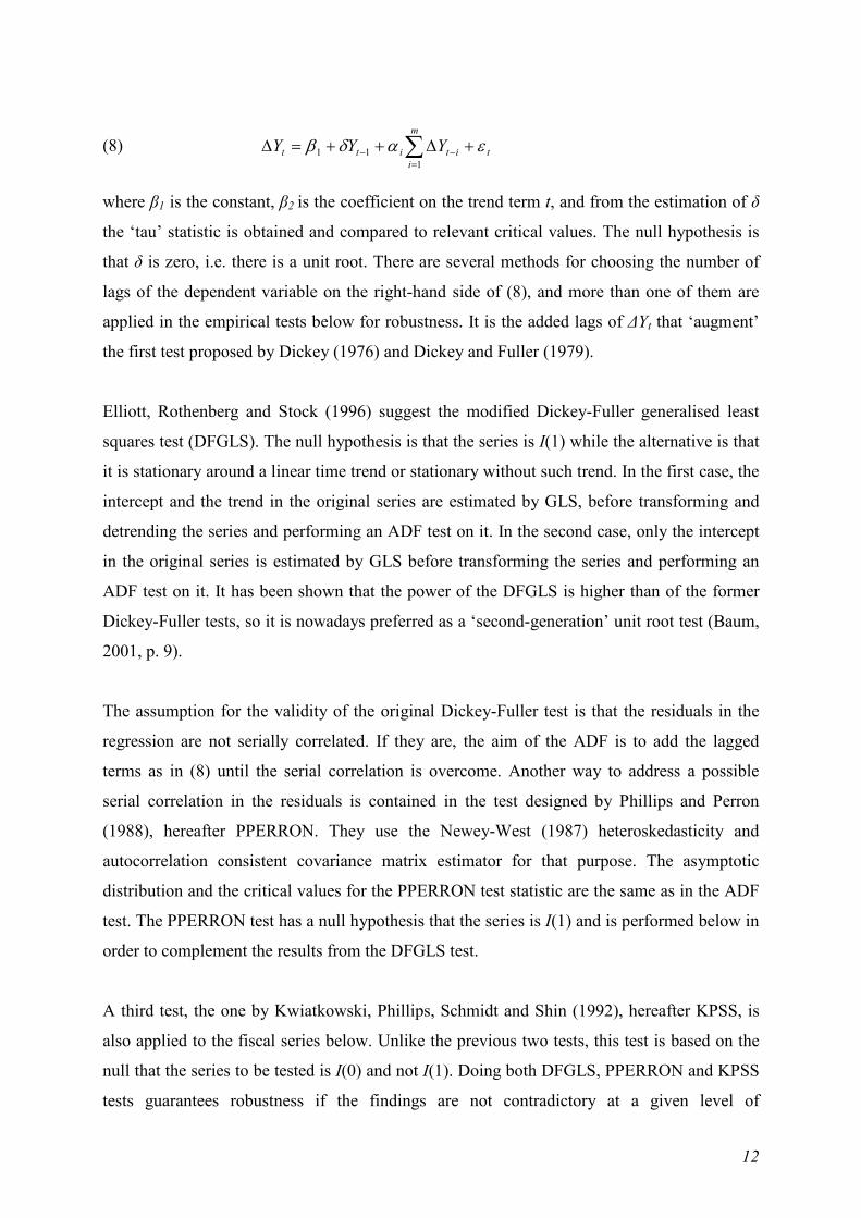
(8) ∑=

−− +∆++=∆m

itititt YYY

111 εαδβ

where β1 is the constant, β2 is the coefficient on the trend term t, and from the estimation of δ

the ‘tau’ statistic is obtained and compared to relevant critical values. The null hypothesis is

that δ is zero, i.e. there is a unit root. There are several methods for choosing the number of

lags of the dependent variable on the right-hand side of (8), and more than one of them are

applied in the empirical tests below for robustness. It is the added lags of ∆Yt that ‘augment’

the first test proposed by Dickey (1976) and Dickey and Fuller (1979).

Elliott, Rothenberg and Stock (1996) suggest the modified Dickey-Fuller generalised least

squares test (DFGLS). The null hypothesis is that the series is I(1) while the alternative is that

it is stationary around a linear time trend or stationary without such trend. In the first case, the

intercept and the trend in the original series are estimated by GLS, before transforming and

detrending the series and performing an ADF test on it. In the second case, only the intercept

in the original series is estimated by GLS before transforming the series and performing an

ADF test on it. It has been shown that the power of the DFGLS is higher than of the former

Dickey-Fuller tests, so it is nowadays preferred as a ‘second-generation’ unit root test (Baum,

2001, p. 9).

The assumption for the validity of the original Dickey-Fuller test is that the residuals in the

regression are not serially correlated. If they are, the aim of the ADF is to add the lagged

terms as in (8) until the serial correlation is overcome. Another way to address a possible

serial correlation in the residuals is contained in the test designed by Phillips and Perron

(1988), hereafter PPERRON. They use the Newey-West (1987) heteroskedasticity and

autocorrelation consistent covariance matrix estimator for that purpose. The asymptotic

distribution and the critical values for the PPERRON test statistic are the same as in the ADF

test. The PPERRON test has a null hypothesis that the series is I(1) and is performed below in

order to complement the results from the DFGLS test.

A third test, the one by Kwiatkowski, Phillips, Schmidt and Shin (1992), hereafter KPSS, is

also applied to the fiscal series below. Unlike the previous two tests, this test is based on the

null that the series to be tested is I(0) and not I(1). Doing both DFGLS, PPERRON and KPSS

tests guarantees robustness if the findings are not contradictory at a given level of

13

significance. This approach to testing for unit roots/stationarity in the total revenue and total

expenditures series is pursued below.

These tests are fairly standard in applied research today but their sometimes low power and

size properties are also admitted. The literature in that respect is vast. Haldrup and Jansson

(2005) review some criticisms of unit root tests and the theoretical advances in increasing

their power and size. Later, Jönsson (2006) and Carrion-i-Silvestre and Sansó (2006) have

discussed the size and power properties of the KPSS stationarity test. Unit root tests with a

null of nonstationarity may lack the power to reject a wrong null when the root of the time

series is ‘close to’ but less than unity. In addition, misspecification regarding a trend or the

numbers of lags may distort the size of the test, in which case a true null may be rejected. This

is a reason why various specifications and tests are compared below.

The revenue-expenditure fiscal sustainability condition may be explored via a number of

cointegration methods, once the individual series are found to be I(1)12. The analysis of long-

run relationships in accordance with the IBC requires an estimation of the cointegrating

vector. Johansen (1988, 1991 and 1995) and Ahn and Reinsel (1990) have considered

efficient estimation based on cointegrated systems fitted in vector error-correction models

(VECM). An alternative model for cointegrated systems, the ‘triangular’ representation,

yields other efficient estimators such as in Saikkonen (1991) and Stock and Watson (1993).

The empirical analysis below employs the dynamic OLS (DOLS) and the dynamic GLS

(DGLS) estimators as proposed by Stock and Watson (1993)13. These estimators are simple to

compute and, in the case when the individual series are I(1) and there is a single cointegrating

vector, they are asymptotically equivalent to the Johansen/Ahn-Reinsel estimator (ibid., p.

784).

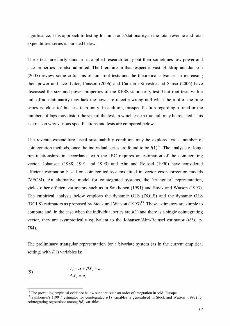
The preliminary triangular representation for a bivariate system (as in the current empirical

setting) with I(1) variables is:

(9) tt

ttt

uX

XY

=∆

++= εβα

12 The prevailing empirical evidence below supports such an order of integration in ‘old’ Europe. 13 Saikkonen’s (1991) estimator for cointegrated I(1) variables is generalised in Stock and Watson (1993) for cointegrating regressions among I(d) variables.

14

where (εt′, ut′)′ is a stationary stochastic process14. In order to control for any correlation

between εt and ut, Saikkonen (1991) and Stock and Watson (1993) suggest augmenting (9)

with differenced leads and lags of the regressor, i.e. the following DOLS regression is

estimated:

(10) t

K

Kkktktt XXY εγβα +∆++= ∑

−=−

where k is the lead/lag order. K should be such that the correlation between εt and ut

disappears for Kk > . There is no unique method for determining the lead/lag order

(Arghyrou and Luintel, 2007, p. 393) but the least-squares estimation of (10) is ‘not feasible if

K is too large compared with the sample size’ (Saikkonen, 1991, p. 13). Stock and Watson

(1993) choose K = 2 or K = 3 for their Monte Carlo samples with 100 or 300 observations,

respectively (ibid., p. 797), and both K = 2 and K = 3 for their empirical data with over 80

years of annual observations (ibid., p. 802). In view of the shorter series of annual data from

the EU14, below the lead/lag order is set to 1.

If the residuals in (10) are autocorrelated, then the DGLS is the correct cointegrating

regression estimator. The construction of the GLS estimator assumes that εt follows an AR(p)

process. Stock and Watson (1993, p. 797 and p. 802) set p = K and that is also the general

approach in the application here, i.e. p = 1. In few cases where the first-order autoregressive

correction is not sufficient to capture the autocorrelation in the errors, the latter are modelled

as an AR(2) for the GLS transformation. The estimation of the autocorrelation structure thus

follows Campbell and Perron (1991, p. 51).

In (10), α and β are the cointegrating parameters; hence the estimated vector, V̂ , is given by

tt XYV βα ˆˆˆ −−= and ‘its stationarity can be checked through any standard unit root test’

(Arghyrou and Luintel, 2007, p. 393).

14 This follows equations (2.1a) and (2.1b) in Stock and Watson (1993, p. 785); an analogous but more general system nesting (9) is presented in Saikkonen (1991, p. 3).

15

3.3. The research strategy

Using the econometric techniques just described, the assessment of fiscal sustainability in

Europe involves the following stages. First, the orders of integration of the series of total

revenues and total expenditures are examined. In the cointegrating equation then the total

revenues are regressed on the total expenditures, applying either the DOLS or, if the residuals

are serially correlated, the DGLS estimators. The null hypothesis of a unit root in the

cointegrating equation is tested, and a number of diagnostic tests are also performed to check

the model specification.

Fiscal sustainability strictly requires a cointegrating vector of (1, -1), so the convergence in

sustainability over time can be inferred from the recursive estimation of the cointegrating

(slope) parameter. That is why the recursive estimates of the coefficient of total expenditures

along with the 95% confidence band are reported, treating 1985 as the start date for the

recursion. If there were any Maastricht/SGP effects or other structural breaks in the

cointegrating relationship, they should be visually detected. The recursive estimation of the

cointegrating (slope) parameter delineates the current study from previous fiscal sustainability

literature and forms an essential part of the research strategy15.

Finally, the Maastricht effect can be tested by estimating the total multiplier of Maastricht

effect through an overall slope dummy for the whole period following the Treaty16. The

analytical framework at this stage mirrors Arghyrou and Luintel (2007). Other things being

equal, a positive coefficient of the slope dummy ‘implies a move towards … strong-form

sustainability because the bubble term converges faster to zero when β � 1 rather than when β

< 1’ (ibid., p. 400); the converse interpretation applies when the same coefficient is estimated

negative.

15 Hatemi-J (2002b) takes a related yet distinctly different step: he provides time varying estimates of the slope coefficient but in a state-space model and where expenditures are regressed on revenues; his empirical analysis covers only one European economy. 16 Thus the break date is exogenously selected.

16

4. DATA AND EMPIRICAL RESULTS

This section demonstrates the empirical analysis of fiscal sustainability in the EU14, the

hypothesized convergence in sustainability over time and the Maastricht effect. The relevant

fiscal data are discussed first.

4.1. Data

The paper uses data on total revenue and total expenditures, both as percent of GDP at market

price. The choice of the two series corresponds to the revenue-expenditure cointegration as

the preferred empirically testable condition for the convergence study strategy.

A key consideration about the data concerns the level of government. The fiscal sustainability

literature often prefers the general government as the most comprehensive level of

government, best revealing the fiscal stance of a country. The Maastricht and SGP deficit and

debt criteria, which are a natural context for ‘old’ Europe’s fiscal sustainability assessment in

a historical perspective, not coincidentally are also set in terms of the general government.

Another consideration regards the frequency of the fiscal series. The choice of annual data is

backed by an econometric argument. Unit root/stationarity and cointegration tests are of little

value if the series are too short to allow for the reversion to a mean or trend equilibrium. The

small-sample bias in traditional time series econometrics is well-documented but some

simulation studies (Hakkio and Rush, 1991b, and Otero and Smith, 2000) have shown that

increasing the frequency of the sample does not significantly raise the test power and a false

null hypothesis is still easily accepted. Neither are the size distortions of the tests alleviated by

increasing the frequency while staying at a relatively short time span: a true null hypothesis is

still easily rejected. With those limitations in mind, annual general government fiscal data are

used here.

Finally, the cut-off date for the series is 2006, being the last year without any traces of the

ensuing financial crisis. In 2007, the French BNP Paribas bank closed three of its hedge funds

which had suffered from their exposures to the US ‘subprime’ mortgage lending markets. The

prices of ‘subprime’-related mortgage backed securities were falling after the collapse of the

housing market, inflicting losses upon financial companies across the globe, including

17

Europe. In August 2007 the European Central Bank started to inject liquidity into the banking

sector. In September 2007 the British bank Northern Rock asked for financial support from

the Bank of England, stirring a bank run in the United Kingdom. The UK government in 2007

raised significantly the deposit guarantees. But as early as in 2006 the fiscal authorities still

had not encountered the coming cyclical downturn, falling tax revenue and rising crisis-

related spending.

The current deep economic crisis is also expected to have affected potential output growth,

causing structural changes in the macroeconomic series. There is insufficient number of

recent observations, however, to estimate the precise nature and timing of any such structural

shifts. All in all, ending the empirical series in 2006 provides for a ‘purer’ data environment

to test if the economies of ‘old’ Europe have in fact been prepared by the Maastricht/SGP

rules for the burden of the forthcoming crisis.

Table 1 presents descriptive statistics for the fiscal variables. The original series were at

current prices and in millions of national currency units. Pre-1999 data for the Euro area

countries are fixed to the Euro at the country’s irrevocable Euro conversion rate.

[Table 1 about here]

4.2. Unit root/stationarity results

The first results from the unit root and stationarity tests are presented in Table 2. A battery of

specifications and tests were applied for robustness. At the conventional confidence intervals

the evidence suggests overwhelmingly that the series of total expenditures and total revenues

in the levels are not stationary for the fourteen countries of this sample. Table 3 displays the

evidence from the same tests but this time performed on the first-differenced series. The

results suggest that the differenced series are I(0) rather than I(1).

[Tables 2 and 3 about here]

18

4.3. Cointegration results

The cointegration analysis is to provide the main evidence for or against fiscal sustainability.

Having established that the fiscal series are I(1), the regression specification from (10) is

applied to the EU14 data, with total revenue the dependent variable and total expenditures the

regressor. The results from the DOLS (DGLS) regression, the unit-root tests for the estimated

cointegrating vector and the set of diagnostics are presented in Table 4, following the research

strategy outlined previously.

[Table 4 about here]

In Austria, Belgium, Denmark, Finland, France, Greece, Ireland, Italy and Spain the

cointegrating coefficient on the expenditures (β) is statistically significant but the unity null is

strongly rejected. The slope parameter is estimated positive and less than 1, and the unit root

in the cointegrating vector is not rejected: hence, weak-form sustainability is confirmed for

these countries.

Non-stationarity of the cointegrating vector is rejected, at various significance levels, in

Germany, the Netherlands, Sweden and the United Kingdom but the cointegrating

coefficients are statistically different from unity, positive and less than 1. Thus, again

evidence for only weak-form sustainability is provided there.

For Portugal, even though the unity null of the slope coefficient cannot be rejected at the 5%

level and its actual estimate is close to 1, the cointegrating vector is not stationary. Portugal

therefore satisfies another weak-form sustainability definition as per Quintos (1995).

The DGLS transformations employ up to second-order autocorrelation corrections. The

diagnostic tests rarely indicate specification problems at the conventional significance levels:

the residuals are normal, serially uncorrelated, homoskedastic and without ARCH effects.

In summary, ‘old’ Europe appears to be no more than weak-form fiscally sustainable. This

evidence broadly confirms Arghyrou and Luintel’s (2007) results from a previous,

geographically more limited, European study exploring Quintos’s (1995) fiscal sustainability

conditions. In view of such results, however, it is important to remember that ‘weak’ fiscal

19

sustainability may in practice place an undue fiscal burden on the public finances of a country

and lead to fiscal unsustainability eventually17. All in all therefore, the full samples from the

last four decades from ‘old’ Europe hardly offer any evidence in favour of the hypothesis that

fiscal sustainability, in a historical perspective, has been achieved before the crisis set in.

The recursive estimation of the cointegrating (slope) coefficient (β) in the DOLS (DGLS)

regression of total revenue on total expenditures is set to uncover evidence for fiscal pressures

and adjustment towards sustainability. In this way, the cointegration analysis incorporates an

assessment of possible gradual convergence in fiscal sustainability in Western Europe18.

Figures 2 - 15 display the recursive estimation of the slope coefficients, including the 95%

confidence bands. The recursions start from 1985, so as to disentangle any positive influence

of Maastricht/SGP on fiscal sustainability: if sustainability has emerged only after 1992, then

such effects can plausibly be confirmed.

[Figures 2 - 15 about here]

The recursive cointegration evidence indicates weak-form sustainability across most of the

countries, with the estimated 95% confidence bands for the coefficients varying between 0

and 1. As long as the upper end of the confidence range for the cointegrating parameter

suffices for such a conclusion, the results suggest possible strong-form sustainability in

Finland in the mid-1980s (Figure 5), France shortly after the start of the recursions ((Figure

6), and Portugal after 1994 (Figure 12). If minding that the 95% confidence band partly lies

outside the (0, 1) interval, however, the charts imply absence of fiscal sustainability in

Portugal during the first half of the recursive period and in the United Kingdom (Figure 15)

before 1991.

17 A note of caution is in order when interpreting the ‘weak’ sustainability evidence. Unless the non-cointegration results come from the low power of the tests, with I(1) series any correlation indicated by the slope coefficient from the revenue-expenditure regression may rather be spurious (see Phillips, 1986). Quintos (1995) ignores this and proves that non-stationarity of the residuals in the revenue-expenditure regression, hence an I(1) debt, is compatible with the IBC. Sustainability may also be in place with debt integrated of order 1, or even higher, in the framework of Bohn (2007) but there, indicatively, the slope coefficient restriction is immaterial. That issue gives a further a reason to regard ‘weak’ sustainability as no sustainability whatsoever: as is the approach adopted in this paper. The weak-form results in Table A1 are too documented as a lack of sustainability. 18 Note that a unity slope coefficient is necessary, but insufficient, to prove (strong-form) fiscal sustainability. Thus, the research strategy here assesses whether the minimum requirement is fulfilled.

20

The estimates of the slope coefficient show that the fiscal stance in Germany generally

improved, despite a slight deterioration after the launch of the Euro (Figure 7). Greece

likewise displays steady improvement throughout the 1990s (Figure 8)19. Again just within

Quintos’s (1995) weak-form definition, there is a marked improvement in fiscal sustainability

in Spain after the country joined the EU in 1986 (Figure 13). For the rest of ‘old’ Europe, the

results demonstrate little or no signs of convergence in fiscal sustainability since 1985.

As for a particular 1992 regime change, only Austria (Figure 2), Germany, Greece and

Portugal display any more visible jumps in the estimated coefficient of the expenditures,

suggesting that Maastricht at least initially spurred a convergence in fiscal sustainability. No

clear positive effect can be seen in Denmark (Figure 4), Ireland (although Figure 9 hints that

the Maastricht Treaty may have stopped the deviation from fiscal sustainability), Italy (Figure

10), the Netherlands (Figure 11), Spain, Sweden (Figure 14), and the United Kingdom.

Conversely, a negative Maastricht effect is rather observed in the cases of Belgium (Figure 3),

Finland and France.

To sum up, no country belonging to ‘old’ Europe satisfies the IBC in the ‘strong’ sense

defined by Quintos (1995) because either the revenue and expenditures are not cointegrated,

or the estimated cointegrating vector is not (1, -1), or both. Such is the evidence from the

cointegration analysis over the full sample periods; the recursive estimation of the coefficient

on the expenditures signifies no convergence in sustainability either.

The recursions also showed little empirical support for a Maastricht Treaty effect. The

hypothesis of a regime change can be addressed explicitly with the estimation of the total

multiplier of Maastricht effect through an overall slope dummy for the whole period after the

(exogenously selected) break in 1992. As in Arghyrou and Luintel (2007), a significantly

positive slope coefficient will then suggest that Maastricht has induced fiscal adjustment

towards the strong-form sustainability. This further view on the EU14 is illustrated by the

empirical results in Table 5, where the specification from (10) is augmented by the structural

shift dummies.

[Table 5 about here]

19 The quality of Greek fiscal data has recently become a target of scepticism.

21

The total multiplier associated with Maastricht turns out to be significantly positive, but its

estimated value suggests only a modest regime change to improve the fiscal outlook after

1992, in Austria, Belgium, Denmark, Germany, Ireland, Portugal, and Spain. The same

Maastricht effect seems only slightly stronger in the cases of Greece and Italy. Finland,

France, the Netherlands and Sweden (a non-EMU country) show a statistically insignificant

total multiplier, thus indicating no fiscal sustainability effect from the Maastricht Treaty. The

estimated Maastricht slope dummy appears significantly negative in the United Kingdom,

confirming the move away from strong-form sustainability after 1992. The UK did not have

to conform to the European convergence criteria in order to adopt the Euro; hence the

Maastricht Treaty may have not been the cause for the negative post-1992 effect on the

country’s government finances.

In all countries except the UK, the overall slope (β + φ) is statistically different from zero and

positive but less than 1, thus implying weak-form fiscal sustainability regardless of whether

the cointegrating vector residuals appear stationary (Austria, Germany, the Netherlands) or

not.

The UK evidence stands out with an estimated coefficient of the overall slope which is

statistically insignificant. Hence, despite rejecting the unit root null in the residuals from the

cointegrating vector, the evidence from this country poses a challenge even to the weak-form

fiscal sustainability definition of Quintos (1995).

All in all, the combined results from Table 4 and Table 5 provide evidence against fiscal

sustainability which is fairly uniform across the fourteen countries and robust in terms of

whether the Maastricht effect is explicitly considered or not. In most cases in ‘old’ Europe,

the Treaty of 1992 has encouraged only negligible adjustments to satisfy the strong-form

definition of long-run fiscal sustainability; sometimes the Maastricht effect is absent or even

significantly negative.

22

5. CONCLUDING REMARKS

A comprehensive statistical assessment of the fiscal performance of ‘old’ Europe during the

last almost four decades hardly offers any evidence in favour of the hypothesis that fiscal

sustainability, in a historical perspective, has been achieved. This verdict conforms to the

majority of previous European-based studies documented in the Annex (Table A1). However,

the recursive cointegration methodology in this paper makes it possible to examine if there

was any convergence in fiscal sustainability over time. It may now be acknowledged that the

fiscal rules imposed to ensure the successful launching and functioning of the monetary union

have not in fact induced national policies compliant with the IBC. This conclusion is all the

more robust since the analysis here is among the few really pan-European fiscal sustainability

studies.

There has always been keen academic interest in the fiscal side of the EMU, the literature

both spurring and shadowing the policies in the run-up to the Euro in the 1990s and the SGP

reform debate in the current decade. As the E(M)U enlarges further and new economies

experience some old compliance challenges, public finances in Europe will remain an area

where theory and policy intersect. The area of public finance sustainability is also topical in

the midst of the economic crisis. What are the policy implications then, if neither Maastricht,

nor the Pact, nor the actual advent of the Euro seem to have mattered in streamlining any

efforts to run public finances in keeping with the intertemporal constraint?

The first implication to note is that the post-2007 crisis has caught ‘old’ Europe fiscally

unprepared. Since the countries over most of the period reviewed have failed the IBC

condition, policy changes were required earlier if the authorities had been keen to restore

long-run sustainability. From today on, the fiscal consolidations will need to be faster and

more ambitious than currently considered.

Unfortunately this suggestion may be alerting but is not straightforwardly translatable into

concrete budgetary policies. Policymakers may intuitively expect that reducing the

government debt is required, implying an increase in revenue or cut in expenditures. But

hardly anything is clear about the size and sign of adjustments needed to achieve a stationary

linear combination between revenues and total expenditures.

23

Whereas the evidence here may be judged more narrowly as just an empirical application of

the proposed sustainability convergence method, it nonetheless sheds new light on the

rationale behind the European fiscal rules. Opponents of the current fiscal regime in Europe

might be tempted to arm themselves with the findings from this paper. A possible neutral

argument, however, could be that the results above do not immediately relate to the efficacy

of the fiscal rules: but rather bear on a claim that the Maastricht and SGP fiscal arrangements

differ from some definitions of long-run sustainability.

24

REFERENCES

Afonso, António (2005) Fiscal Sustainability: The Unpleasant European Case. FinanzArchiv

61, 19-44.

Afonso, António and Christophe Rault (2007a) Should We Care for Structural Breaks When

Assessing Fiscal Sustainability? Economics Bulletin 3, 1-9.

Afonso, António and Christophe Rault (2007b) What Do We Really Know about Fiscal

Sustainability in the EU? A Panel Data Diagonostic. Working Paper Series No. 820:

European Central Bank.

Ahmed, Shaghil and John H. Rogers (1995) Government Budget Deficits and Trade Deficits:

Are Present Value Constraints Satisfied in Long-Term Data? Journal of Monetary

Economics 36, 351-374

Ahn, Sung K. and Gregory C. Reinsel (1990) Estimation for Partially Nonstationary

Multivariate Autoregressive Models. Journal of the American Statistical Association

85, 813-823.

Arghyrou, Michael G. and Kul B. Luintel (2007) Government Solvency: Revisiting Some

EMU Countries. Journal of Macroeconomics 29, 387-410.

Artis, Michael and Massimiliano Marcellino (1998) Fiscal Solvency and Fiscal Forecasting in

Europe. CEPR Discussion Papers No. 1836: CEPR.

Baglioni, Angelo and Umberto Cherubini (1993) Intertemporal Budget Constraint and Public

Debt Sustainability: The Case of Italy. Applied Economics 25, 275-283.

Bajo-Rubio, Oscar, Carmen Díaz-Roldán and Vicente Esteve (2004) Searching for Threshold

Effects in the Evolution of Budget Deficits: An Application to the Spanish Case.

Economics Letters 82, 239-243.

Bajo-Rubio, Oscar, Carmen Díaz-Roldán and Vicente Esteve (2006) Is the Budget Deficit

Sustainable When Fiscal Policy is Non-linear? The Case of Spain. Journal of

Macroeconomics 28, 596-608.

Baum, Christopher F. (2001) Stata: The Language of Choice for Time-Series Analysis? The

Stata Journal 1, 1-16.

Blanchard, Olivier Jean (1990) Suggestions for a New Set of Fiscal Indicators. OECD

Economics Department Working Papers No. 79: OECD.

Blot, Christophe and Francisco Serranito (2006) Convergence of Fiscal Policies in EMU: A

Unit-Root Tests Analysis with Structural Break. Applied Economics Letters 13, 211-

216.

25

Bohn, Henning (2007) Are Stationarity and Cointegration Restrictions Really Necessary for

the Intertemporal Budget Constraint? Journal of Monetary Economics 54, 1837-1847.

Bravo, Ana Bela Santos and Antonio Luis Silvestre (2002) Intertemporal Sustainability of

Fiscal Policies: Some Tests for European Countries. European Journal of Political

Economy 18, 517-528.

Burnside, Craig (2005) Fiscal Sustainability in Theory and Practice: A Handbook. The World

Bank.

Campbell, John Y. and Pierre Perron (1991) Pitfalls and Opportunities: What

Macroeconomists Should Know about Unit Roots. NBER Working Papers Series

Technical Working Paper No. 100.

Caporale, Guglielmo Maria (1995) Bubble Finance and Debt Sustainability: A Test of the

Government's Intertemporal Budget Constraint. Applied Economics 27, 1135-1143.

Carrion-i-Silvestre, Josep Lluís and Andreu Sansó (2006) Testing the Null of Cointegration

with Structural Breaks. Oxford Bulletin of Economics and Statistics 68, 623-646.

Chalk, Nigel Andrew and Richard Hemming (2000) Assessing Fiscal Sustainability in Theory

and Practice. Working Paper No. 00/81: International Monetary Fund.

Cipollini, Andrea (2001) Testing For Government Intertemporal Solvency: A Smooth

Transition Error Correction Model Approach. The Manchester School 69, 643-655.

Claeys, Peter (2007) Sustainability of EU Fiscal Policies: A Panel Test. Journal of Economic

Integration 22, 112 - 127.

Considine, John and Liam A. Gallagher (2008) UK Debt Sustainability: Some Nonlinear

Evidence and Theoretical Implications. The Manchester School 76, 320-335.

Corsetti, Giancarlo and Nouriel Roubini (1991) Fiscal Deficits, Public Debt, and Government

Solvency: Evidence from OECD Countries. Journal of the Japanese and International

Economies 5, 354-380.

De Bandt, Olivier and Francesco Paolo Mongelli (2000) Convergence of Fiscal Policies in the

Euro Area. Working Paper Series No. 20: European Central Bank.

De Haan, Jakob, Jan-Egbert Sturm and Olaf De Groot (2004) Policy Adjustments and

Sustainability of Public Finances in the Netherlands. paper presented at the

CESifo/LBI conference on Sustainability of Public Debt in Munich, 22-23 October

2004.

Dickey, David A. (1976) Estimation and Hypothesis Testing in Nonstationary Time Series.

PhD thesis, Iowa: Iowa State University.

Dickey, David A. and Wayne A. Fuller (1979) Distribution of the Estimators for

26

Autoregressive Time Series With a Unit Root. Journal of the American Statistical

Association 74, 427-431.

EC (2006) Public Finances in EMU - 2006. European Economy 3.

Elliott, Graham, Thomas J. Rothenberg and James H. Stock (1996) Efficient Tests for an

Autoregressive Unit Root. Econometrica 64, 813-836.

Engle, Robert F. and Clive W. J. Granger (1987) Co-integration and Error Correction:

Representation, Estimation, and Testing. Econometrica 55, 251-276.

Engsted, Tom and Niels Haldrup (1999) Multicointegration in Stock-Flow Models. Oxford

Bulletin of Economics and Statistics 61, 237-254.

Fatás, Antonio and Ilian Mihov (2003) On Constraining Fiscal Policy Discretion in EMU.

Oxford Review of Economic Policy 19, 112-131.

Feve, Patrick and Pierre-Yves Henin (2000) Assessing Effective Sustainability of Fiscal

Policy within the G–7. Oxford Bulletin of Economics and Statistics 62, 175-195.

Getzner, Michael, Ernst Glatzer and Reinhard Neck (2001) On the Sustainability of Austrian

Budgetary Policies. Empirica 28, 21-40.

Granger, Clive W. J. and T.H. Lee (1990) Multicointegration. In G.F. Rhodes and T.B.

Fomby (eds.), Advances in Econometrics: Cointegration, Spurious Regression, and

Unit Roots, pp. 71-84. Greenwich: JAI Press.

Green, Christopher J., Mark J. Holmes and Tadeusz Kowalski (2001) Poland: A Successful

Transition to Budget Sustainability? Emerging Markets Review 2, 161-183.

Greiner, Alfred and Willi Semmler (1999) An Inquiry Into the Sustainability Of German

Fiscal Policy: Some Time-Series Tests. Public Finance Review 27, 220-238.

Hakkio, Craig S. and Mark Rush (1991a) Is the Budget Deficit 'Too Large?' Economic

Inquiry 29, 429-445.

Hakkio, Craig S. and Mark Rush (1991b) Cointegration: How Short is the Long Run? Journal

of International Money and Finance 10, 571-581.

Haldrup, Niels and Michael Jansson (2005) Improving Size and Power in Unit Root Testing.

Working Papers No. 2: Department of Economics, University of Aarhus.

Hamilton, James D. and Marjorie A. Flavin (1986) On the Limitations of Government

Borrowing: A Framework for Empirical Testing. The American Economic Review 76,

808-819

Hatemi-J, Abdulnasser (2002a) Fiscal Policy in Sweden: Effects of EMU Criteria

Convergence. Economic Modelling 19, 121-136.

Hatemi-J, Abdulnasser (2002b) Is the Government's Intertemporal Budget Constraint Fulfilled

27

in Sweden? An Application of the Kalman Filter. Applied Economics Letters 9, 433 -

439.

Haug, Alfred A. (1991) Cointegration and Government Borrowing Constraints: Evidence for

the United States. Journal of Business and Economic Statistics 9, 97-101.

Johansen, Søren (1988) Statistical Analysis of Cointegration Vectors. Journal of Economic

Dynamics and Control 12, 231-254.

Johansen, Søren (1991) Estimation and Hypothesis Testing of Cointegration Vectors in

Gaussian Vector Autoregressive Models. Econometrica 59, 1551-1580.

Johansen, Søren (1995) Likelihood-based inference in cointegrated vector autoregressive

models. Oxford University Press.

Jönsson, Kristian P. (2006) Finite-Sample Stability of the KPSS Test. Working Papers No.

23: Lund University, Department of Economics.

Kalyoncu, Hüseyin (2005) Fiscal Policy Sustainability: Test of Intertemporal Borrowing

Constraints. Applied Economics Letters 12, 957 - 962.

Kirchgässner, Gebhard and Silika Prohl (2006) Sustainability of Swiss Fiscal Policy. CESifo

Working Paper No. 1689: March.

Konstantinou, Panagiotis T. (2004) Balancing the Budget Through Revenue or Spending

Adjustments? The Case of Greece. Journal of Economic Development 29, 81-105.

Kremers, Jeroen J. M. (1989) U.S. Federal Indebtedness and the Conduct of Fiscal Policy.

Journal of Monetary Economics 23, 219-238.

Kwiatkowski, Denis, Peter C. B. Phillips, Peter Schmidt and Yongcheol Shin (1992) Testing

the Null Hypothesis of Stationarity Against the Alternative of a Unit Root. Journal of

Econometrics 54, 159-178.

Leachman, Lori, Alan Bester, Guillermo Rosas and Peter Lange (2005) Multicointegration

and the Sustainability of Fiscal Practices. Economic Inquiry 43, 454-466.

Ley, Eduardo (2003) Fiscal (and External) Sustainability. Public Economics No. 0310007:

EconWPA.

Liu, Peter and Evan Tanner (1995) Intertemporal Solvency and Breaks in the US Deficit

Process: A Maximum-Likelihood Cointegration Approach. Applied Economics Letters

2, 231-235.

Llorca, Matthieu and Srdjan Redzepagic (2008) Debt Sustainability in the EU New Member

States: Empirical Evidence from a Panel of Eight Central and East European

Countries. Post-Communist Economies 20, 159 - 172.

MacDonald, Ronald and AEH Speight (1990) The Intertemporal Government Budget

28

Constraint in the U.K., 1961-1986. The Manchester School 58, 329-347.

MacKinnon, James G. (1991) Critical Values for Cointegration Tests. In Robert F. Engle and

Clive W. J. Granger (eds.), Long-Run Economic Relationships: Readings in

Cointegration, pp. 267-276. Oxford: Oxford University Press.

Makrydakis, Stelios, Elias Tzavalis and Athanassios Balfoussias (1999) Policy Regime

Changes and the Long-Run Sustainability of Fiscal Policy: An Application to Greece.

Economic Modelling 16, 71-86.

Marinheiro, Carlos Fonseca (2006) The Sustainability of Portuguese Fiscal Policy from a

Historical Perspective. Empirica 33, 155-179.

McCallum, Bennett T. (1984) Are Bond-Financed Deficits Inflationary? A Ricardian

Analysis. Journal of Political Economy 92, 123-135.

Newey, Whitney K. and Kenneth D. West (1987) A Simple, Positive Semi-Definite,

Heteroskedasticity and Autocorrelation Consistent Covariance Matrix. Econometrica

55, 703-708.

O'Connell, Stephen A. and Stephen P. Zeldes (1988) Rational Ponzi Games. International

Economic Review 29, 431-450.

Otero, Jesus and Jeremy Smith (2000) Testing for Cointegration: Power versus Frequency of

Observation-Further Monte Carlo Results. Economics Letters 67, 5-9.

Papadopoulos, Athanasios P. and Moise G. Sidiropoulos (1999) The Sustainability of Fiscal

Policies in the European Union. International Advances in Economic Research 5, 289-

307.

Payne, James E. (1997) International Evidence on the Sustainability of Budget Deficits.

Applied Economics Letters 4, 775 - 779.

Pesaran, M. Hashem, Yongcheol Shin and Richard J. Smith (2001) Bounds Testing

Approaches to the Analysis of Level Relationships. Journal of Applied Econometrics

16, 289-326.

Phillips, Peter C. B. (1986) Understanding Spurious Regressions in Econometrics. Journal of

Econometrics 33, 311-340.

Phillips, Peter C. B. and Pierre Perron (1988) Testing for a Unit Root in Time Series

Regression. Biometrika 75, 335-346.

Prazmowski, Peter A. (2005) A Recursive Cointegration Test Using the Kalman Filter and Its

Application to Fiscal Equilibrium in the Dominican Republic. Applied Economics

Letters 12, 155 - 160.

Prohl, Silika and Friedrich G. Schneider (2006) Sustainability of Public Debt and Budget

29

Deficit: Panel cointegration analysis for the European Union Member countries.

Economics working papers 2006-10: Department of Economics, Johannes Kepler

University Linz, Austria.

Quintos, Carmela E. (1995) Sustainability of the Deficit Process with Structural Shifts.

Journal of Business and Economic Statistics 13, 409-417.

Saikkonen, Pentti (1991) Asymptotically Efficient Estimation of Cointegration Regressions.

Econometric Theory 7, 1-21.

Stock, James H. and Mark W. Watson (1993) A Simple Estimator of Cointegrating Vectors in

Higher Order Integrated Systems. Econometrica 61, 783-820.

Tanner, Evan and Peter Liu (1994) Is the Budget Deficit "Too Large"?: Some Further

Evidence. Economic Inquiry 32, 511-518.

Trehan, Bharat and Carl E. Walsh (1988) Common Trends, the Government's Budget

Constraint, and Revenue Smoothing. Journal of Economic Dynamics and Control 12,

425-444.

Trehan, Bharat and Carl E. Walsh (1991) Testing Intertemporal Budget Constraints: Theory

and Applications to U.S. Federal Budget and Current Account Deficits. Journal of

Money, Credit and Banking 23, 206-223.

Uctum, Merih, Thom Thurston and Remzi Uctum (2006) Public Debt, the Unit Root

Hypothesis and Structural Breaks: A Multi-Country Analysis. Economica 73, 129-

156.

Uctum, Merih and Michael Wickens (2000) Debt and Deficit Ceilings, and Sustainability of

Fiscal Policies: An Intertemporal Analysis. Oxford Bulletin of Economics and

Statistics 62, 197-222.

Vanhorebeek, Filip and Paul Van Rompuy (1995) Solvency and Sustainability of Ffiscal

Policies in the EU. De Economist 143, 457-473.

Vieira, Carlos (1999) The Sustainability of Fiscal Policy: An Application to the European

Union. unpublished PhD thesis, Loughborough: Loughborough University.

Westerlund, Joakim and Silika Prohl (2008) Panel Cointegration Tests of the Sustainability

Hypothesis in Rich OECD Countries. Applied Economics, First published on: 08

January 2008 (iFirst), 1-10.

30

ANNEX: EUROPEAN FISCAL SUSTAINABILITY STUDIES Table A1 here documents the emerging European fiscal sustainability literature. It contains

empirical works within the econometric ‘backward-looking’ strand of literature. Research into

fiscal sustainability in Europe began only after the North American studies and gained

momentum since the 1990s. The existing findings are based on diverse research strategies and

are often contradictory across papers and samples.

As long as this paper aims to expand the eclectic empirical evidence for Europe, the selection

follows the geographical criterion. As such, Table A1 intends to serve as a comprehensive

European fiscal sustainability catalogue, enriching similar attempts in Vieira (1999) and

Afonso (2005).

31

Table A1.

Som

e ex

istin

g em

piri

cal e

vide

nce

abou

t fis

cal s

usta

inab

ility

in E

urop

e Pa

per

Cou

ntry

(per

iod)

D

ata

freq

uenc

y E

cono

met

ric

test

s(1)

Sust

aina

bilit

y(2)

Afo

nso

(200

5)

EU

15 (1

970-

2003

) A

nnua

l U

nit r

oot t

ests

for f

irst

dif

fere

nce

of d

ebt,

unit

root

s w

ith b

reak

s fo

r deb

t, co

inte

grat

ion

for r

even

ues

and

expe

nditu

res

(inc

ludi

ng

stru

ctur

al s

hift

test

s)

No

Afo

nso

and

Rau

lt (2

007a

) E

U15

(197

0-20

06)

Ann

ual

Coi

nteg

ratio

n fo

r rev

enue

s an

d ex

pend

iture

s (w

ith a

nd

with

out b

reak

s)

Yes

Afo

nso

and

Rau

lt (2

007b

) E

U15

(197

0-20

06)

Ann

ual

Coi

nteg

ratio

n fo

r rev

enue

s an

d ex

pend

iture

s,

unit

root

test

s fo

r fir

st d

iffe

renc

e of

deb

t (w

ith a

nd

with

out b

reak

s)

Yes

: for

the

pane

l N

o: fo

r som

e te

sts

for t

he

indi

vidu

al c

ount

ries

A

hmed

and

Rog

ers

(199

5)

US

(179

2-19

92) a

nd U

K

(169

2-19

92)

Ann

ual

Coi

nteg

ratio

n fo

r rev

enue

s, e

xpen

ditu

res

and

debt

Y

es

Arg

hyro

u an

d L

uint

el (2

007)

G

reec

e (1

970:

1-19

98:3

), It

aly

(196

2:2-

1997

:4),

Irel

and

and

Net

herl

ands

(1

957:

1-19

98:4

)

Qua

rter

ly

Coi

nteg

ratio

n fo

r rev

enue

s an

d ex

pend

iture

s (w

ith a

nd

with

out b

reak

s)

Yes

Art

is a

nd M

arce

llino

(199

8)

EU

15 w

ithou

t Gre

ece

and

Lux

embo

urg

(per

iod

vari

es a

cros

s co

untr

ies

betw

een

1963

and

199

4)

Ann

ual

Uni

t roo

t tes

ts fo

r (un

)dis

coun

ted

debt

(gro

ss/n

et)

Yes

: for

dis

coun

ted

debt

in

Bel

gium

, Spa

in a

nd It

aly

(net

) and

in A

ustr

ia,

Bel

gium

, Net

herl

ands

and

U

K (g

ross

) N

o: a

ll ot

her c

ount

ries

/deb

t de

fini

tions

B

aglio

ni a

nd C

heru

bini

(199

3)

Ital

y (1

979:

1-19

91:5

) M

onth

ly

Uni

t roo

t tes

ts fo

r deb

t N

o B

ajo-

Rub

io, D

íaz-

Rol

dán

and

Est

eve

(200

4)

Spai

n (1

964-

2001

) A

nnua

l T

hres

hold

aut

oreg

ress

ive

mod

el o

f the

ove

rall

budg

et

bala

nce/

GD

P ra

tio

Yes

Baj

o-R

ubio

, Día

z-R

oldá

n an

d E

stev

e (2

006)

Sp

ain

(196

4-20

03, 1

982:

1-20

04:1

)

Ann

ual a

nd

quar

terl

y N

onlin

ear t

hres

hold

coi

nteg

ratio

n fo

r rev

enue

s an

d ex

pend

iture

s Y

es

Bra

vo a

nd S

ilves

tre

(200

2)

11 E

U c

ount

ries

(196

0-20

00)

Ann

ual

Coi

nteg

ratio

n fo

r rev

enue

s an

d ex

pend

iture

s N

o

Cap

oral

e (1

995)

10

EU

cou

ntri

es (p

erio

d va

ries

acr

oss

coun

trie

s be

twee

n 19

60 a

nd 1

991)

Ann

ual a

nd s

emi-

annu

al (f

or th

e di

ffer

ent c

ount

ries

)

Uni

t roo

t tes

ts fo

r deb

t N

o: D

enm

ark,

Ger

man

y,

Gre

ece

and

Ital

y Y

es: t

he re

st

Cip

ollin

i (20

01)

UK

(196

3:1-

1997

:3)

Qua

rter

ly

Uni

t roo

t tes

ts fo

r ove

rall

bala

nce,

co

inte

grat

ion

for r

even

ues

and

expe

nditu

res

(and

a re

gim

e sw

itch

to a

djus

t tow

ards

line

ar c

oint

egra

ting

rela

tions

hip)

No

(unl

ess

regi

me

shif

t in

the

face

of l

arge

imba

lanc

es)

Cla

eys

(200

7)

EU

15 w

ithou

t L

uxem

bour

g (1

970-

2001

) A

nnua

l U

nit r

oot t

ests

for d

ebt,

unit

root

test

s fo

r ove

rall

bala

nce,

co

inte

grat

ion

for r

even

ues,

exp

endi

ture

s an

d in

tere

st

paym

ents

Yes

: for

the

pane

l N

o: fo

r som

e te

sts

for t

he

indi

vidu

al c

ount

ries

32

Pape

r C

ount

ry (p

erio

d)

Dat

a fr

eque

ncy

Eco

nom

etri

c te

sts(1

) Su

stai

nabi

lity(2

) C

onsi

dine

and

Gal

lagh

er (2

008)

U

K (1

919-

2001

) A

nnua

l E

xpon

entia

l sm

ooth

tran

sitio

n au

tore

gres

sive

mod

el o

f th

e de

bt/G

DP

ratio

Y

es

Cor

setti

and

Rou

bini

(199

1)

18 O

EC

D c

ount

ries

(1

960-

1989

) A

nnua

l U

nit r

oot t

ests

for d

isco

unte

d de

bt,

unit

root

test

s fo

r unc

ount

ed d

ebt,

unit

root

test

s fo

r ove

rall

bala

nce

No:

Bel

gium

, Gre

ece,

Ir

elan

d, It

aly

and

Net

herl

ands

Y

es: t

he re

st

De

Haa

n, S

turm

and

De

Gro

ot

(200

4)

Net

herl

ands

(194

8-20

03)

Ann

ual

Uni

t roo

t tes

ts fo

r def

icit,

co

inte

grat

ion

for r

even

ues

and

expe

nditu

res

Yes

Feve

and

Hen

in (2

000)

G

7 (v

ario

us, u

nspe

cifi

ed)

Sem

i-an

nual

U

nit r

oot t

ests

for d

ebt

Yes

: UK

N

o: th

e re

st

Get

zner

, Gla

tzer

and

Nec

k (2

001)

A

ustr

ia (1

960-

1999

) A

nnua

l U

nit r

oot t

ests

for d

isco

unte

d de

bt,

unit

root

test

s fo

r dis

coun

ted

prim

ary

and

over

all d

efic

it Y

es: 1

960-

1974

N

o: 1

975-

1999

G

reen

, Hol

mes

and

Kow

alsk

i (2

001)

Po

land

(199

1:1-

1998

:3)

Mon

thly

U

nit r

oot t

ests

for o

vera

ll ba

lanc

e,

coin

tegr

atio

n fo

r rev

enue

s an

d ex

pend

iture

s Y

es

Gre

iner

and

Sem

mle

r (19

99)

Ger

man

y (1

955-

1994

) A

nnua

l U

nit r

oot t

ests

for d

isco

unte

d de

bt,

unit

root

test

s fo

r dis

coun

ted

prim

ary

and

over

all d

efic

it N

o

Hat

emi-

J (2

002a

) Sw

eden

(196

3:1-

2000

:1)

Qua

rter

ly

Coi

nteg

ratio

n fo

r rev

enue

s, e

xpen

ditu

res,

deb

t and

pri

vate

co

nsum

ptio

n Y

es

Hat

emi-

J (2

002b

) Sw

eden

(196

3:1-

2000

:1)

Qua

rter

ly

Coi

nteg

ratio

n fo

r tax

es a

nd e

xpen

ditu

res

incl

udin

g in

tere

st p

aym

ents

(tim

e va

ryin

g co

effi

cien

t mod

el)

Yes

Kal

yonc

u (2

005)

T

urke

y (1

970-

2001

), M

exic

o, S

outh

Afr

ica,

So

uth

Kor

ea a

nd th

e Ph

ilipp

ines

(per

iod

vari

es

acro

ss c

ount

ries

bet

wee

n 19

70 a

nd 2

003)

Ann

ual (

Tur

key)

an

d qu

arte

rly

(the

re

st)

Coi

nteg

ratio

n fo

r rev

enue

s an

d ex

pend

iture

s N

o

Kir

chgä

ssne

r and

Pro

hl (2

006)

Sw

itzer

land

(190

0-20

02)

Ann

ual

Uni

t roo

t tes

ts fo

r deb

t and

def

icit

(with

and

with

out a

br

eak)

, co

inte

grat

ion

for r

even

ues

and

expe

nditu

res

Yes

: ove

r ent

ire

peri

od

No:

bef

ore

1940

and

aft

er

1945

K

onst

antin

ou (2

004)

G

reec

e (1

970:

1-19

97:1

) Q

uart

erly

U

nit r

oot t

ests

for d

efic

it,

coin

tegr

atio

n fo

r rev

enue

s an

d ex

pend

iture

s N

o

Lea

chm

an, B

este

r, R

osas

and

L

ange

(200

5)

15 in

dust

rial

ised

cou

ntri

es

(196

0-19

98)

Ann

ual

Coi

nteg

ratio

n (a

nd m

ultic

oint

egra

tion)

for r

even

ues

and

expe

nditu

res

Yes

: fro

m m

ultic

oint

egra

tion

test

s, N

orw

ay a

nd U

K

No:

all

othe

r cou

ntri

es/te

sts

Llo

rca

and

Red

zepa

gic

(200

8)

8 E

U a

cces

sion

cou

ntri

es

(199

9:1-

2006

:1)

Qua

rter

ly

Uni

t roo

t tes

ts fo

r deb

t, un

it ro

ot te

sts

for o

vera

ll ba

lanc

e,

unit

root

test

s fo

r rev

enue

s an

d ex

pend

iture

s,

Coi

nteg

ratio

n fo

r rev

enue

s an

d ex

pend

iture

s

Yes

Mac

Don

ald

and

Spei

ght (

1990

) U

K (1

961-

1986

) A

nnua

l C

oint

egra

tion

for d

ebt a

nd p

rim

ary

defi

cit

Inco

nclu

sive

M

akry

daki

s, T

zava

lis a

nd

Bal

fous

sias

(199

9)

Gre

ece

(195

8-19

95)

Ann

ual

Uni

t roo

t tes

ts fo

r dis

coun

ted

debt

(with

/with

out a

bre

ak)

No

33

Pape

r C

ount

ry (p

erio

d)

Dat

a fr

eque

ncy

Eco

nom

etri

c te

sts(1

) Su

stai

nabi

lity(2

) M

arin

heir

o (2

006)

Po

rtug

al (1

852-

2003

) A

nnua

l U

nit r

oot t

ests

for f

irst

dif

fere

nce

of d

ebt,

unit

root

test

s fo

r def

icit,

co

inte

grat

ion

for r

even

ues

and

expe

nditu

res

(inc

ludi

ng

stru

ctur

al s

hift

test

s)

Yes

: 190

3-20

03

No:

bef

ore

1903

N

o: a

fter

197

5

Papa

dopo

ulos

and

Sid

irop

oulo

s (1

999)

B

elgi

um, G

reec

e, It

aly,

Po

rtug

al a

nd S

pain

(per

iod

vari

es a

cros

s co

untr

ies

betw

een

1961

and

199

5)

Ann

ual

Uni

t roo

t tes

ts fo

r def

icit

(with

and

with

out b

reak

s),

coin

tegr

atio

n fo

r rev

enue

s an

d ex

pend

iture

s Y

es: G

reec

e, P

ortu

gal a

nd

Spai

n N

o: B

elgi

um a

nd It

aly

Payn

e (1

997)

G

7 co

untr

ies

(per

iod

vari

es a

cros

s co

untr

ies

betw

een

1949

and

199

4)

Ann

ual

Coi

nteg

ratio

n fo

r rev

enue

s an

d ex

pend

iture

s Y

es: G

erm

any

No

or in

conc

lusi

ve: t

he re

st

Proh

l and

Sch

neid

er (2

006)

E

U15

(197

0-20

04)

Ann

ual

Coi

nteg

ratio

n fo

r rev

enue

s an

d ex

pend

iture

s N

o U

ctum

, Thu

rsto

n an

d U

ctum

(2

006)

G

7 an

d se

lect

ed L

atin

A

mer

ica

and

Asi

a co

untr

ies

(197

0-20

02)

Ann

ual

Uni

t roo

t tes

ts fo

r dis

coun

ted

debt

(with

and

with

out a

br

eak)

Y

es: w

ith a

bre

ak, F

ranc

e,

Ital

y, T

urke

y an

d U

K

No:

all

othe

r Eur

opea

n co

untr

ies

with

or w

ithou

t te

stin

g fo

r uni

t roo

ts w

ith a

br

eak

Uct

um a

nd W

icke

ns (2

000)

11

EU

cou

ntri

es a

nd U

S (p

erio

d va

ries

acr

oss

coun

trie

s be

twee

n 19

65

and

1994

)

Ann

ual

Uni

t roo

t tes

ts fo

r (di

scou

nted

) deb

t Y

es: D

enm

ark,

Fra

nce,

Ir

elan

d an

d N

ethe

rlan

ds

No:

the

rest

Van

hore

beek

and

Van

Rom

puy

(199

5)

8 E

U c

ount

ries

(197

0-19

94),

and

Bel

gium

se

para

tely

(187

0-19

93)

Ann

ual

Uni

t roo

t tes

ts fo

r deb

t, un

it ro

ot te

sts

for o

vera

ll de

fici

t

Yes

: Ger

man

y an

d Fr

ance

N

o or

inco

nclu

sive

: the

rest

Vie

ira

(199

9)

Bel

gium

, Ger

man

y,

Fran

ce, I

taly

, Net

herl

ands

an

d U

K (p

erio

d va

ries

ac

ross

cou

ntri

es b

etw

een

1950

and

199

6)

Ann

ual a

nd

quar

terl

y U

nit r

oot t

ests

for d

efic

it (w

ith a

nd w

ithou

t bre

aks)

, co

inte

grat

ion

for r

even

ues

and

expe

nditu

res

Yes

: Ger

man

y N

o: th

e re

st

Wes

terl

und

and

Proh

l (20

08)

8 O

EC

D c

ount

ries

Q

uart

erly

C

oint

egra

tion

for r

even

ues

and

expe

nditu

res

(with

bre

aks)

Y

es

Not

es:

(1) F

urth

er te

sts

depe

ndin

g on

the

pape

r’s

rese

arch

que

stio

ns m

ay h

ave

been

per

form

ed.

(2) T

he c

oncl

usio

n re

gard

ing

only

Eur

opea

n su

stai

nabi

lity

if th

e sa

mpl

e al

so c

ompr

ises

non

-Eur

ope

coun

trie

s. W

here

test

ed f

or, w

eak-

form

sus

tain

abili

ty f

ollo

win

g Q

uint

os (1

995)

is h

ere

docu

men

ted

as a

lack

of s

usta

inab

ility

.

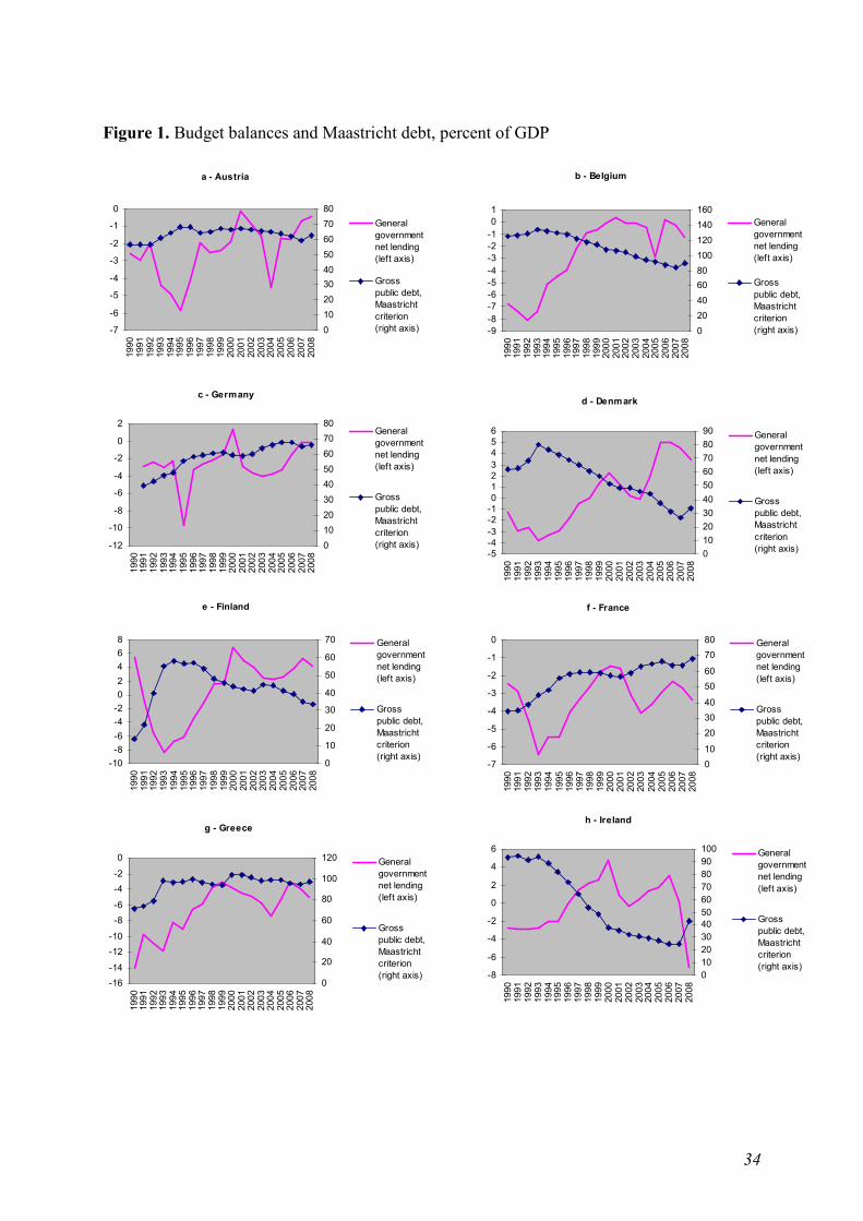
34

Figure 1. Budget balances and Maastricht debt, percent of GDP

a - Austria

-7

-6

-5

-4

-3

-2

-1

0

1990

1991

1992

1993

1994

1995

1996

1997

1998

1999

2000

2001

2002

2003

2004

2005

2006

2007

2008

0

10

20

30

40

50

60

70

80

Generalgovernmentnet lending(left axis)

Grosspublic debt,Maastrichtcriterion(right axis)

b - Belgium

-9-8-7-6-5-4-3-2-101

1990

1991

1992

1993

1994

1995

1996

1997

1998

1999

2000

2001

2002

2003

2004

2005

2006

2007

2008

0

20

40

60

80

100

120

140

160Generalgovernmentnet lending(left axis)

Grosspublic debt,Maastrichtcriterion(right axis)

c - Germany

-12

-10

-8

-6

-4

-2

0

2

1990

1991

1992

1993

1994

1995

1996

1997

1998

1999

2000

2001

2002

2003

2004

2005

2006

2007

2008

0

10

20

30

40

50

60

70

80Generalgovernmentnet lending(left axis)

Grosspublic debt,Maastrichtcriterion(right axis)

d - Denmark

-5-4-3-2-10123456

1990

1991

1992

1993

1994

1995

1996

1997

1998

1999

2000

2001

2002

2003

2004

2005

2006

2007

2008

010203040

5060708090 General

governmentnet lending(left axis)

Grosspublic debt,Maastrichtcriterion(right axis)

e - Finland

-10-8-6

-4-202

468

1990

1991

1992

1993

1994

1995

1996

1997

1998

1999

2000

2001

2002

2003

2004

2005

2006

2007

2008

0

10

20

30

40

50

60

70 Generalgovernmentnet lending(left axis)

Grosspublic debt,Maastrichtcriterion(right axis)

f - France

-7

-6

-5

-4

-3

-2

-1

0

1990

1991

1992

1993

1994

1995

1996

1997

1998

1999

2000

2001

2002

2003

2004

2005

2006

2007

2008

0

10

20

30

40

50

60

70

80 Generalgovernmentnet lending(left axis)

Grosspublic debt,Maastrichtcriterion(right axis)

g - Greece

-16

-14

-12

-10

-8

-6

-4

-2

0

1990

1991

1992

1993

1994

1995

1996

1997

1998

1999

2000

2001

2002

2003

2004

2005

2006

2007

2008

0

20

40

60

80

100

120 Generalgovernmentnet lending(left axis)

Grosspublic debt,Maastrichtcriterion(right axis)

h - Ireland

-8

-6

-4

-2

0

2

4

6

1990

1991

1992

1993

1994

1995

1996

1997

1998

1999

2000

2001

2002

2003

2004

2005

2006

2007

2008

0102030405060708090100 General

governmentnet lending(left axis)

Grosspublic debt,Maastrichtcriterion(right axis)

35

Figure 1. Budget balances and Maastricht debt, percent of GDP (continued)

Source: OECD.

i - Italy

-14

-12

-10

-8

-6

-4

-2

0

1990

1991

1992

1993

1994

1995

1996

1997

1998

1999

2000

2001

2002

2003

2004

2005

2006

2007

2008

0

20

40

60

80

100

120

140 Generalgovernmentnet lending(left axis)

Grosspublic debt,Maastrichtcriterion(right axis)

j - Netherlands

-10

-8

-6

-4

-2

0

2

4

1990

1991

1992

1993

1994

1995

1996

1997

1998

1999

2000

2001

2002

2003

2004

2005

2006

2007

2008

0

10

2030

40

50

6070

80

90 Generalgovernmentnet lending(left axis)

Grosspublic debt,Maastrichtcriterion(right axis)

k - Portugal

-8

-7

-6

-5

-4

-3

-2

-1

0

1990

1991

1992

1993

1994

1995

1996

1997

1998

1999

2000

2001

2002

2003

2004

2005

2006

2007

2008

0

10

20

30

40

50

60

70Generalgovernmentnet lending(left axis)

Grosspublic debt,Maastrichtcriterion(right axis)

l - Spain

-8

-6

-4

-2

0

2

4

1990

1991

1992

1993

1994

1995

1996

1997

1998

1999

2000

2001

2002

2003

2004

2005

2006

2007

2008

0

10

20

30

40

50

60

70

80Generalgovernmentnet lending(left axis)

Grosspublic debt,Maastrichtcriterion(right axis)

m - Sweden

-12

-10

-8

-6

-4

-2

0

2

4

6

1990

1991

1992

1993

1994

1995

1996

1997

1998

1999

2000

2001

2002

2003

2004

2005

2006

2007

2008

0

10

20

30

40

50

60

70

80Generalgovernmentnet lending(left axis)

Grosspublic debt,Maastrichtcriterion(right axis)

n - United Kingdom

-10

-8

-6

-4

-2

0

2

4

6

1990

1991

1992

1993

1994

1995

1996

1997

1998

1999

2000

2001

2002

2003

2004

2005

2006

2007

2008

0

10

20

30

40

50

60Generalgovernmentnet lending(left axis)

Grosspublic debt,Maastrichtcriterion(right axis)

36

Figure 2. Austria: convergence in fiscal sustainability

0

0.1

0.2

0.3

0.4

0.5

0.6

0.7

0.8

0.9

1985 1986 1987 1988 1989 1990 1991 1992 1993 1994 1995 1996 1997 1998 1999 2000 2001 2002 2003 2004 2005 2006

Cointegrating parameter(total expenditures/GDP)

95% confidence band

Figure 3. Belgium: convergence in fiscal sustainability

-0.2

-0.1

0

0.1

0.2

0.3

0.4

0.5

0.6

1985 1986 1987 1988 1989 1990 1991 1992 1993 1994 1995 1996 1997 1998 1999 2000 2001 2002 2003 2004 2005 2006

Cointegrating parameter(total expenditures/GDP)

95% confidence band

`

Figure 4. Denmark: convergence in fiscal sustainability

0

0.2

0.4

0.6

0.8

1

1.2

1985 1986 1987 1988 1989 1990 1991 1992 1993 1994 1995 1996 1997 1998 1999 2000 2001 2002 2003 2004 2005 2006

Cointegrating parameter(total expenditures/GDP)

95% confidence band

`

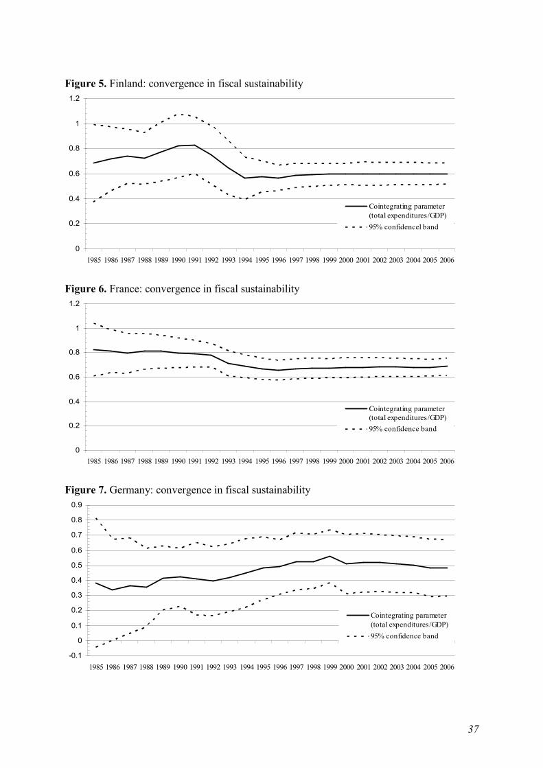
37

Figure 5. Finland: convergence in fiscal sustainability

0

0.2

0.4

0.6

0.8

1

1.2

1985 1986 1987 1988 1989 1990 1991 1992 1993 1994 1995 1996 1997 1998 1999 2000 2001 2002 2003 2004 2005 2006

Cointegrating parameter(total expenditures/GDP)

95% confidencel band

Figure 6. France: convergence in fiscal sustainability

0

0.2

0.4

0.6

0.8

1

1.2

1985 1986 1987 1988 1989 1990 1991 1992 1993 1994 1995 1996 1997 1998 1999 2000 2001 2002 2003 2004 2005 2006

Cointegrating parameter(total expenditures/GDP)

95% confidence band

Figure 7. Germany: convergence in fiscal sustainability

-0.1

0

0.1

0.2

0.3

0.4

0.5

0.6

0.7

0.8

0.9

1985 1986 1987 1988 1989 1990 1991 1992 1993 1994 1995 1996 1997 1998 1999 2000 2001 2002 2003 2004 2005 2006

Cointegrating parameter(total expenditures/GDP)

95% confidence band

38

Figure 8. Greece: convergence in fiscal sustainability

0

0.1

0.2

0.3

0.4

0.5

0.6

0.7

0.8

1985 1986 1987 1988 1989 1990 1991 1992 1993 1994 1995 1996 1997 1998 1999 2000 2001 2002 2003 2004 2005 2006

Cointegrating parameter(total expenditures/GDP)

95% confidence band

Figure 9. Ireland: convergence in fiscal sustainability

0

0.1

0.2

0.3

0.4

0.5

0.6

0.7

0.8

0.9

1985 1986 1987 1988 1989 1990 1991 1992 1993 1994 1995 1996 1997 1998 1999 2000 2001 2002 2003 2004 2005 2006

Cointegrating parameter(total expenditures/GDP)

95% confidence band

Figure 10. Italy: convergence in fiscal sustainability

0

0.2

0.4

0.6

0.8

1

1.2

1985 1986 1987 1988 1989 1990 1991 1992 1993 1994 1995 1996 1997 1998 1999 2000 2001 2002 2003 2004 2005 2006

Cointegrating parameter(total expenditures/GDP)

95% confidence band

39

Figure 11. Netherlands: convergence in fiscal sustainability

0

0.1

0.2

0.3

0.4

0.5

0.6

0.7

0.8

0.9

1985 1986 1987 1988 1989 1990 1991 1992 1993 1994 1995 1996 1997 1998 1999 2000 2001 2002 2003 2004 2005 2006

Cointegrating parameter(total expenditures/GDP)

95% confidence band

Figure 12. Portugal: convergence in fiscal sustainability

0

0.2

0.4

0.6

0.8

1

1.2

1.4

1985 1986 1987 1988 1989 1990 1991 1992 1993 1994 1995 1996 1997 1998 1999 2000 2001 2002 2003 2004 2005 2006

Cointegrating parameter(total expenditures/GDP)

95% confidence band

Figure 13. Spain: convergence in fiscal sustainability

0

0.1

0.2

0.3

0.4

0.5

0.6

0.7

0.8

0.9

1985 1986 1987 1988 1989 1990 1991 1992 1993 1994 1995 1996 1997 1998 1999 2000 2001 2002 2003 2004 2005 2006

Cointegrating parameter(total expenditures/GDP)

95% confidence band

40

Figure 14. Sweden: convergence in fiscal sustainability

0

0.1

0.2

0.3

0.4

0.5

0.6

0.7

1985 1986 1987 1988 1989 1990 1991 1992 1993 1994 1995 1996 1997 1998 1999 2000 2001 2002 2003 2004 2005 2006

Cointegrating parameter(total expenditures/GDP)

95% confidence band

Figure 15. United Kingdom: convergence in fiscal sustainability

-1.5

-1

-0.5

0

0.5

1

1.5

2

2.5

3

3.5

1985 1986 1987 1988 1989 1990 1991 1992 1993 1994 1995 1996 1997 1998 1999 2000 2001 2002 2003 2004 2005 2006

Cointegrating parameter(total expenditures/GDP)

95% confidence band

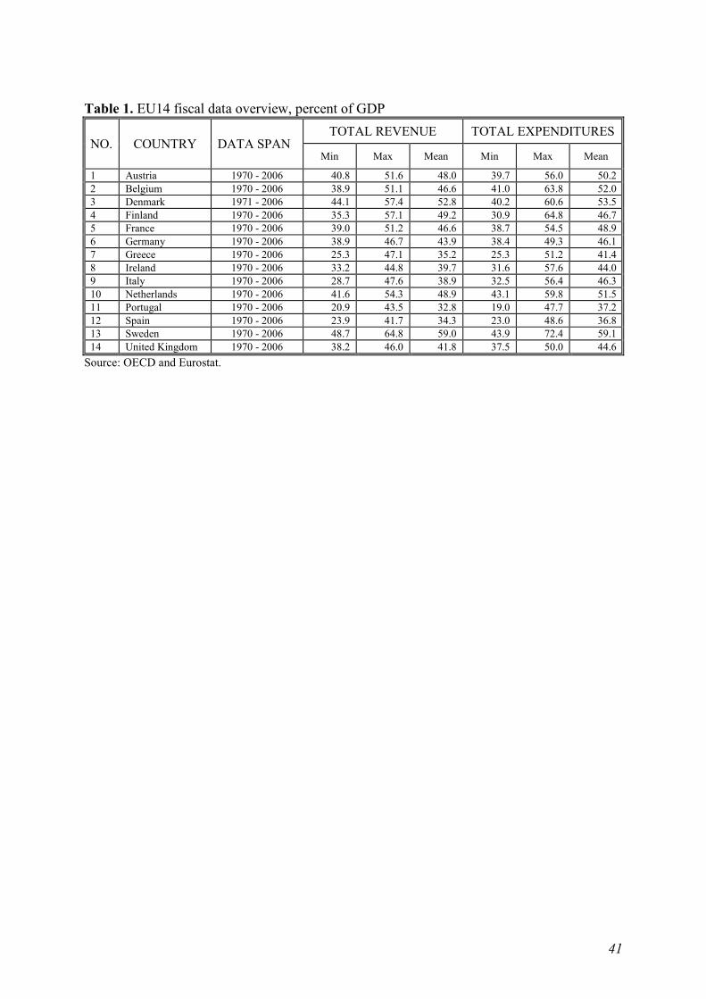
41

Table 1. EU14 fiscal data overview, percent of GDP

NO. COUNTRY DATA SPAN TOTAL REVENUE TOTAL EXPENDITURES

Min Max Mean Min Max Mean

1 Austria 1970 - 2006 40.8 51.6 48.0 39.7 56.0 50.2 2 Belgium 1970 - 2006 38.9 51.1 46.6 41.0 63.8 52.0 3 Denmark 1971 - 2006 44.1 57.4 52.8 40.2 60.6 53.5 4 Finland 1970 - 2006 35.3 57.1 49.2 30.9 64.8 46.7 5 France 1970 - 2006 39.0 51.2 46.6 38.7 54.5 48.9 6 Germany 1970 - 2006 38.9 46.7 43.9 38.4 49.3 46.1 7 Greece 1970 - 2006 25.3 47.1 35.2 25.3 51.2 41.4 8 Ireland 1970 - 2006 33.2 44.8 39.7 31.6 57.6 44.0 9 Italy 1970 - 2006 28.7 47.6 38.9 32.5 56.4 46.3 10 Netherlands 1970 - 2006 41.6 54.3 48.9 43.1 59.8 51.5 11 Portugal 1970 - 2006 20.9 43.5 32.8 19.0 47.7 37.2 12 Spain 1970 - 2006 23.9 41.7 34.3 23.0 48.6 36.8 13 Sweden 1970 - 2006 48.7 64.8 59.0 43.9 72.4 59.1 14 United Kingdom 1970 - 2006 38.2 46.0 41.8 37.5 50.0 44.6

Source: OECD and Eurostat.

42

Table 2. Unit root/stationarity tests: total expenditures and total revenues (levels)

Country Series Tests with trend(1) Tests without trend(1) DFGLS (2,6) DFGLS

(3,6) KPSS(4) PPERRON

(4,5) DFGLS

(2,6) DFGLS

(3,6) KPSS (4) PPERRON

(4,5) Austria te -0.495 (1) -0.495 (1) 0.424* -1.969 -0.542 (1) -0.542 (1) 1.07* -4.345

tr -0.426 (1) -0.426 (1) 0.421* -2.133 -0.352 (1) -0.352 (1) 1.39* -4.187

Belgium te -1.580 (2) -1.580 (2) 0.254* -4.190 -1.405 (2) -1.405 (2) 0.254 -5.266

tr -1.410 (1) -1.410 (1) 0.248* -4.844 -0.008 (1) -0.008 (1) 1.23* -3.937

Denmark te -1.474 (1) -1.474 (1) 0.347* -3.307 -1.186 (1) -1.186 (1) 0.902* -4.722

tr -1.447 (1) 0.893 (2) 0.249* -5.991 -0.654 (1) -0.350 (2) 1.06* -2.306

Finland te -2.119 (1) -1.276 (2) 0.204** -4.675 -0.800 (2) -0.800 (2) 0.881* -4.077

tr -0.272 (1) -0.272 (1) 0.345* -5.135 0.153 (1) 0.153 (1) 1.51* -3.959

France te -1.574 (1) -0.823 (4) 0.345* -4.978 -0.203 (1) -0.368 (9) 1.61* -2.496

tr -1.266 (1) -1.266 (1) 0.333* -5.025 0.685 (1) 0.685 (1) 1.64* -1.855

Germany te -1.777 (1) -1.777 (1) 0.125*** -10.011 -0.877 (1) -0.877 (1) 0.576** -10.116

tr -1.621 (1) -1.621 (1) 0.128*** -9.886 -0.706 (1) -0.706 (1) 0.74* -9.510

Greece te -0.611 (1) -0.611 (1) 0.41* -0.979 -0.152 (1) -0.152 (1) 1.71* -2.088

tr -2.284 (1) -2.284 (1) 0.118 -9.677 -0.082 (1) -0.082 (1) 1.79* -0.929

Ireland te -1.462 (1) -1.462 (1) 0.364* -4.891 -0.947 (1) -0.947 (1) 1.16* -1.446

tr -1.536 (1) -1.536 (1) 0.366* -6.271 -1.045 (1) -1.045 (1) 0.763* -4.417

Italy te -0.999 (1) -0.999 (1) 0.444* -2.750 -0.229 (1) -0.229 (1) 1.27* -3.331

tr -1.330 (1) -1.330 (1) 0.31* -4.028 0.197 (1) 0.197 (1) 1.81* -1.207

Netherlands te -0.867 (1) -0.867 (1) 0.429* -3.853 -0.961 (1) -0.961 (1) 0.497** -3.489

tr -1.258 (1) -1.258 (1) 0.411* -5.383 -1.204 (1) -1.204 (1) 0.493** -4.876

Portugal te -1.072 (1) -1.072 (1) 0.365* -5.007 0.340 (1) 0.340 (1) 1.65* -2.539

tr -3.087*** (1) -1.867 (2) 0.193** -16.249*** 0.482 (1) 0.482 (1) 1.88* -0.912

Spain te -0.847 (1) -0.847 (1) 0.448* -1.161 -0.479 (1) -0.479 (1) 1.26* -2.798

tr -0.938 (1) -0.938 (1) 0.439* -1.960 0.364 (1) 0.364 (1) 1.64* -1.668

Sweden te -0.806 (1) -0.806 (1) 0.376* -4.025 -0.771 (1) -0.771 (1) 0.673** -5.425

tr -0.403 (1) -0.403 (1) 0.424* -4.084 -0.543 (1) -0.543 (1) 0.881* -5.725

United Kingdom

te -2.349 (1) -2.349 (1) 0.128*** -10.629 -2.104 (1) -2.104 (1) 0.548** -8.288

tr -3.021 (1) -1.950 (2) 0.0987 -13.985 -1.207 (2) -1.207 (2) 0.544** -11.619***

Notes: te and tr stand for total expenditures and total revenues, respectively, as shares of GDP. *, ** and *** denote rejection of the null at 1%, 5% and 10%. In DGFLS, the 5% and 10% critical

values are from Cheung and Lai (1995), while the 1% critical values are interpolated from the ones presented by Elliott, Rothenberg and Stock (1996). In KPSS, the critical values are taken from Kwiatkowski et al. (1992). In PPERRON, the critical values are linearly interpolated from the ones in Fuller (1976).

(1) Both tests with and without a trend include a constant term. (2) Lag order selected according to the minimum Schwarz information criterion

(3) Lag order selected according to the minimum Ng-Perron (2001) modified Akaike information criterion. (4) Same lag order used as determined by either the modified Akaike information criterion if lag at most 3 there, or if otherwise: by the minimum Schwarz information criterion from the DFGLS test. In PPERRON, that is set to correspond to Newey-West truncation lags window used in calculating the standard error (i.e. correction for serial correlation of up to that lag order). (5) The rho statistic in the PPERRON test, H0: rho = 1. (6) The brackets report the number of lags selected for each test statistic.

43

Table 3. Unit root/stationarity tests: total expenditures and total revenues (first differences)

Country Series Tests with trend(1) Tests without trend(1) DFGLS (2,6) DFGLS (3,6) KPSS(4) PPERRON

(4,5) DFGLS

(2,6) DFGLS

(3,6) KPSS (4) PPERRON

(4,5) Austria ∆te -3.740**(1) -3.740** (1) 0.0348 -37.359* -2.817* (1) -1.093 (6) 0.699** -30.013*

∆tr -5.840* (1) -5.840* (1) 0.0298 -39.287* -3.648* (1) 0.087 (7) 0.606** -33.880*

Belgium ∆te -2.347 (1) -2.347 (1) 0.131*** -37.363* -2.051 (1) -2.051 (1) 0.531** -32.455*

∆tr -3.201***(1) -2.079 (2) 0.0926 -39.520* -3.196* (1) -2.019 (2) 0.276 -38.191*

Denmark ∆te -3.895* (1) -3.895* (1) 0.0434 -24.464* -3.908* (1) -3.908* (1) 0.349*** -21.789*

∆tr -4.093* (1) -0.963 (8) 0.0805 -38.255* -3.733* (1) -0.862 (8) 0.15 -38.370*

Finland ∆te -3.391** (1) -3.391** (1) 0.0677 -18.409*** -3.046* (1) -3.046* (1) 0.24 -17.174**

∆tr -4.397* (1) -4.397* (1) 0.0357 -33.346* -2.720* (1) -0.055 (8) 0.311 -30.813*

France ∆te -3.657** (3) -2.731 (1) 0.0435 -23.723** -2.583** (1) -2.583** (1) 0.199 -22.341*

∆tr -3.608** (1) -2.544 (2) 0.0631 -30.413* -3.136* (1) -2.15*** (2) 0.164 -30.565*

Germany ∆te -3.259*** (1) -1.462 (5) 0.091 -29.115* -2.600** (1) -0.848 (5) 0.278 -26.838*

∆tr -3.330*** (1) -1.445 (6) 0.0931 -33.907* -2.362***(1) -0.464 (6) 0.29 -31.169*

Greece ∆te -4.056* (1) -0.890 (8) 0.0924 -43.209* -3.378* (1) -0.537 (8) 0.401*** -40.932*

∆tr -3.279*** (1) -2.343 (2) 0.0811 -30.431* -3.220* (1) -1.067 (7) 0.0845 -30.828*

Ireland ∆te -3.346*** (1) -3.346***(1) 0.0908 -25.961* -2.934* (1) -1.796 (4) 0.22 -25.232*

∆tr -3.998* (1) -2.683 (2) 0.081 -37.935* -3.039* (1) -1.053 (5) 0.095 -38.117*

Italy ∆te -2.809 (1) -2.022 (2) 0.0893 -34.205* -2.081 (1) -1.443 (2) 0.446*** -30.847*

∆tr -3.407** (1) -1.626 (5) 0.0998 -34.115* -3.303* (1) -1.504 (5) 0.178 -33.275*

Netherlands ∆te -3.026 (1) -2.371 (2) 0.115 -35.242* -2.308***(1) -0.781 (7) 0.533** -30.602*

∆tr -2.981 (1) -0.896 (7) 0.154** -29.746* -2.302***(1) -0.726 (5) 0.485** -25.735*

Portugal ∆te -4.168* (1) -4.168*(1) 0.0405 -30.670* -4.036* (1) -4.036* (1) 0.286 -28.605*

∆tr -5.376* (1) -1.037 (8) 0.0446 -33.810* -4.334* (1) -0.723 (8) 0.0607 -33.806*

Spain ∆te -2.958 (1) -2.958 (1) 0.0909 -24.790* -2.14***(1) -0.578 (7) 0.6** -20.500*

∆tr -2.925 (1) -1.944 (3) 0.1 -32.963* -2.864* (1) -1.908 (3) 0.299 -32.165*

Sweden ∆te -3.246*** (1) -3.246***(1) 0.0442 -34.009* -2.506**(1) -2.051 (2) 0.354*** -31.132*

∆tr -3.651**(1) -3.651** (1) 0.0299 -30.380* -1.747 (1) 0.595 (8) 0.493** -26.608*

United Kingdom

∆te -2.871 (1) -2.871 (1) 0.0806 -22.270** -2.871* (1) -2.871* (1) 0.0901 -22.093*

∆tr -3.932* (1) -3.932* (1) 0.0453 -26.336* -2.918* (1) -1.087 (6) 0.0768 -26.115

Notes: ∆te and ∆tr stand for the first differences of total expenditures and total revenues, respectively, as shares of GDP.

*, ** and *** denote rejection of the null at 1%, 5% and 10%. In DGFLS, the 5% and 10% critical values are from Cheung and Lai (1995), while the 1% critical values are interpolated from the ones presented by Elliott, Rothenberg and Stock (1996). In KPSS, the critical values are taken from Kwiatkowski et al. (1992). In PPERRON, the critical values are linearly interpolated from the ones in Fuller (1976).

(1) Both tests with and without a trend include a constant term. (2) Lag order selected according to the minimum Schwarz information criterion

(3) Lag order selected according to the minimum Ng-Perron (2001) modified Akaike information criterion. (4) Same lag order used as determined by either the modified Akaike information criterion if lag at most 3 there, or if otherwise: by the minimum Schwarz information criterion from the DFGLS test. In PPERRON, that is set to correspond to Newey-West truncation lags window used in calculating the standard error (i.e. correction for serial correlation of up to that lag order). (5) The rho statistic in the PPERRON test, H0: rho = 1. (6) The brackets report the number of lags selected for each test statistic.

44

Table 4. C

oint

egra

tion

anal

ysis

with

out b

reak

s C

OU

NTR

Y A

T

BE

D

K

FI

FR

DE

G

R

IE

IT

NL

PT

E

S SE

G

B

D

GL

S (1

)1 DG

LS

(2)1

DG

LS

(1)1 D

GL

S (1

)1 DG

LS

(1)1 D

GL

S (1

)1 DG

LS

(1)1 D

GL

S (1

)1 DG

LS

(1)1 D

GL

S (2

)1 D

GL

S (1

)1 DG

LS

(1)1 D

GL

S (2

)1 D

GL

S (2

)1 E

stim

ated

equ

atio

n:

TRt =

α +

βTE

t + ε

t

α

0.16

0 (0

.026

)*

0.40

1 (0

.021

)*

0.18

6 (0

.047

)*

0.21

5 (0

.020

)*

0.13

5 (0

.017

)*

0.21

7 (0

.042

)*

0.08

4 (0

.017

)*

0.21

9 (0

.012

)*

0.01

5 (0

.026

) 0.

156

(0.0

21)*

-0

.021

(0

.017

) 0.

075

(0.0

13)*

0.

374

(0.0

31)*

0.

200

(0.0

36)*

TE

0.64

0 (0

.050

)*

0.14

0 (0

.039

)*

0.64

7 (0

.085

)*

0.60

1 (0

.041

)*

0.68

5 (0

.034

)*

0.48

3 (0

.091

)*

0.66

0 (0

.037

)*

0.40

0 (0

.025

)*

0.82

2 (0

.053

)*

0.64

6 (0

.039

)*

0.92

9 (0

.040

)*

0.73

8 (0

.033

)*

0.37

6 (0

.051

)*

0.48

6 (0

.081

)*

F

-Wal

d te

st, H

0: β

= 0

[p-v

alue

] 16

3.03

[0

.00]

* 12

.71

[0.0

0]*

57.4

1 [0

.00]

* 21

1.74

[0

.00]

* 41

0.91

[0

.00]

* 28

.36

[0.0

0]*

321.

37

[0.0

0]*

245.

92

[0.0

0]*

237.

87

[0.0

0]*

267.

54

[0.0

0]*

529.

61

[0.0

0]*

486.

52

[0.0

0]*

55.3

0 [0

.00]

* 35

.84

[0.0

0]*

F

-Wal

d te

st, H

0: β

= 1

[p-v

alue

] 51

.54

[0.0

0]*

477.

45

[0.0

0]*

17.1

3 [0

.00]

* 93

.06

[0.0

0]*

87.0

7 [0

.00]

* 32

.44

[0.0

0]*

85.6

1 [0

.00]

* 55

5.00

[0

.00]

* 11

.11

[0.0

0]*

80.5

1 [0

.00]

* 3.

06

[0.0

9]**

* 61

.29

[0.0

0]*

152.

76

[0.0

0]*

40.0

1 [0

.00]

*

t-A

DF

on

tε̂

{la

g or

der}

[5%

cri

tical

val

ue]

-2.7

16

{0}

[-3.

510]

-1.9

15

{0}

[-3.

510]

-2.3

37

{1}

[-3.

521]

-2.5

93

{0}

[-3.

510]

-2.6

98

{1}

[-3.

516]

-3.8

61**

{0

} [-

3.51

0]

-1.1

54

{0}

[-3.

510]

-2.5

44

{0}

[-3.

510]

-1.0

35

{0}

[-3.

510]

-4.5

66*

{3}

[-3.

527]

-2.8

06

{0}

[-3.

510]

-0.5

04

{0}

[-3.

510]

-3.1

81**

* {2

} [-

3.52

1]

-3.6

56**

{1

} [-

3.51

6]

Mis

spec

ific

atio

n te

sts

(p-v

alue

s)

B

reus

ch-G

odfr

ey L

M F

-tes

t

for 1

st o

rder

aut

ocor

rela

tion

0.94

0.

25

0.62

0.

67

0.85

0.

76

0.39

0.

92

0.26

0.

07

0.68

0.

69

0.25

0.

22

Ja

rque

-Ber

a C

hi2 te

st

fo

r nor

mal

ity

0.61

0.

13

0.21

0.

45

0.58

0.

83

0.95

0.

89

0.90

0.

89

0.49

0.

00

0.77

0.

81

E

ngle

’s L

M C

hi2 te

st

fo

r AR

CH

0.

09

0.94

0.

36

0.69

0.

08

0.42

0.

51

0.52

0.

75

0.03

0.

52

0.87

0.

46

0.85

W

hite

’s C

hi2 te

st

fo

r het

eros

keda

stic

ity

0.58

0.

30

0.93

0.

38

0.60

0.

32

0.16

0.

23

0.28

0.

23

0.31

0.

12

0.33

0.

31

Su

stai

nabi

lity

infe

renc

e W

eak-

form

Wea

k-fo

rm W

eak-

form

Wea

k-fo

rm W

eak-

form

Wea

k-fo

rm W

eak-

form

Wea

k-fo

rm W

eak-

form

Wea

k-fo

rm W

eak-

form

Wea

k-fo

rm W

eak-

form

Wea

k-fo

rm

Not

es:

Stan

dard

err

ors

in p

aren

thes

es. A

nnua

l dat

a fr

om 1

970

(197

1 in

Den

mar

k) to

200

6.

1 DG

LS

orde

r of t

he a

utoc

orre

latio

n co

rrec

tion.

*,

**

and

***

deno

te s

igni

fica

nce

at th

e 1%

, 5%

and

10%

leve

l, re

spec

tivel

y.

TR

and

TE

sta

nd fo

r tot

al re

venu

e an

d to

tal e

xpen

ditu

res,

resp

ectiv

ely,

as

shar

es o

f GD

P.

AD

F is

the

Aug

men

ted

Dic

key-

Fulle

r te

st (

lag

orde

r se

lect

ed u

sing

the

min

imum

Sch

war

z in

form

atio

n cr

iteri

on;

coin

tegr

atio

n te

st c

ritic

al v

alue

s fr

om

Mac

Kin

non,

199

1, T

able

1).

45

Table 5. C

oint

egra

tion

anal

ysis

with

a b

reak

C

OU

NTR

Y A

T

BE

D

K

FI

FR

DE

G

R

IE

IT

NL

PT

E

S SE

G

B

D

GL

S (1

)1 DG

LS

(1)1

DG

LS

(1)1 D

GL

S (1

)1 DG

LS

(1)1 D

GL

S (1

)1 DG

LS

(1)1 D

GL

S (1

)1 DG

LS

(1)1 D

GL

S (2

)1 D

GL

S (2

)1 DG

LS

(1)1 D

GL

S (2

)1 D

GL

S (1

)1 E

stim

ated

equ

atio

n:

TRt =

α +

βTE

t + φ

(DtT

E t) +

ε t

α

0.18

3 (0

.024

)*

0.28

6 (0

.029

)*

0.25

1 (0

.045

)*

0.20

8 (0

.029

)*

0.12

3 (0

.024

)*

0.27

7 (0

.051

)*

0.17

2 (0

.020

)*

0.18

8 (0

.022

)*

0.07

9 (0

.023

)*

0.18

9 (0

.028

)*

0.03

3 (0

.024

) 0.

097

(0.0

12)*

0.

368

(0.0

32)*

0.

322

(0.0

55)*

TE

0.58

6 (0

.047

)*

0.32

6 (0

.052

)*

0.50

4 (0

.085

)*

0.61

9 (0

.067

)*

0.71

1 (0

.049

)*

0.34

7 (0

.110

)*

0.37

6 (0

.052

)*

0.45

7 (0

.043

)*

0.62

8 (0

.050

)*

0.59

0 (0

.050

)*

0.74

0 (0

.063

)*

0.65

6 (0

.032

)*

0.39

1 (0

.052

)*

0.22

9 (0

.118

)***

D

*TE

(D =

1 in

199

2-20

06,

0

othe

rwis

e)

0.02

0 (0

.006

)*

0.06

9 (0

.009

)*

0.04

9 (0

.012

)*

-0.0

07

(0.0

21)

-0.0

05

(0.0

07)

0.01

6 (0

.006

)**

0.13

2 (0

.018

)*

0.03

1 (0

.018

)***

0.

105

(0.0

15)*

-0

.018

(0

.011

) 0.

087

(0.0

15)*

0.

044

(0.0

11)*

-0

.014

(0

.010

) -0

.045

(0

.013

)*

F

-Wal

d te

st, H

0: β

+ φ

= 0

[p-v

alue

] 17

9.64

[0

.00]

* 47

.98

[0.0

0]*

47.1

9 [0

.00]

* 13

5.00

[0

.00]

* 25

2.37

[0

.00]

* 11

.69

[0.0

0]*

144.

07

[0.0

0]*

69.7

5 [0

.00]

* 25

7.95

[0

.00]

* 97

.63

[0.0

0]*

239.

55

[0.0

0]*

548.

66

[0.0

0]*

52.0

1 [0

.00]

* 2.

07

[0.1

6]

F

-Wal

d te

st, H

0: β

+ φ

= 1

[p-v

alue

] 76

.00

[0.0

0]*

113.

34

[0.0

0]*

30.8

2 [0

.00]

* 53

.99

[0.0

0]*

43.9

4 [0

.00]

* 35

.79

[0.0

0]*

135.

44

[0.0

0]*

76.4

4 [0

.00]

* 34

.19

[0.0

0]*

54.7

7 [0

.00]

* 10

.44

[0.0

0]*

101.

41

[0.0

0]*

141.

48

[0.0

0]*

40.6

3 [0

.00]

*

t-A

DF

on

tε̂

{la

g or

der}

[5%

cri

tical

val

ue]

-3.9

88**

* {1

} [-

3.99

2]

-2.2

83

{0}

[-3.

985]

-2.6

37

{1}

[-4.

000]

-2.5

57

{0}

[-3.

985]

-2.6

65

{1}

[-3.

992]

-3.9

60**

* {0

} [-

3.98

5]

-2.5

45

{0}

[-3.

985]

-2.8

32

{0}

[-3.

985]

-2.5

15

{0}

[-3.

985]

-5.0

37*

{3}

[-4.

008]

-3.1

87

{0}

[-3.

985]

-0.8

88

{0}

[-3.

985]

-3.0

08

{2}

[-4.

000]

-3.7

67**

* {1

} [-

3.99

2]

Mis

spec

ific

atio

n te

sts

(p-v

alue

s)

B

reus

ch-G

odfr

ey L

M F

-tes

t

for 1

st o

rder

aut

ocor

rela

tion

0.83

0.

34

0.48

0.

67

0.88

0.

63

0.68

0.

95

0.69

0.

07

0.78

0.

57

0.19

0.

46

Ja

rque

-Ber

a C

hi2 te

st

fo

r nor

mal

ity

0.06

0.

00

0.00

0.

48

0.55

0.

84

0.40

0.

72

0.03

0.

14

0.53

0.

06

0.80

0.

98

E

ngle

’s L

M C

hi2 te

st

fo

r AR

CH

0.

26

0.64

0.

45

0.66

0.

08

0.70

0.

79

0.88

0.

36

0.76

0.

23

0.97

0.

32

0.34

W

hite

’s C

hi2 te

st

fo

r het

eros

keda

stic

ity

0.38

0.

20

0.27

0.

23

0.39

0.

27

0.27

0.

20

0.21

0.

42

0.42

0.

25

0.42

0.

45

Su

stai

nabi

lity

infe

renc

e W

eak-

form

Wea

k-fo

rm W

eak-

form

Wea

k-fo

rm W

eak-

form

Wea

k-fo

rm W

eak-

form

Wea

k-fo

rm W

eak-

form

Wea

k-fo

rm W

eak-

form

Wea

k-fo

rm W

eak-

form

N

o su

stain

abili

ty

Not

es:

Stan

dard

err

ors

in p

aren

thes

es. A

nnua

l dat

a fr

om 1

970

(197

1 in

Den

mar

k) to

200

6.

1 DG

LS

orde

r of t

he a

utoc

orre

latio

n co

rrec

tion.

*,

**

and

***

deno

te s

igni

fica

nce

at th

e 1%

, 5%

and

10%

leve

l, re

spec

tivel

y.

TR

and

TE

sta

nd fo

r tot

al re

venu

e an

d to

tal e

xpen

ditu

res,

resp

ectiv

ely,

as

shar

es o

f GD

P.

AD

F is

the

Aug

men

ted

Dic

key-

Fulle

r te

st (

lag

orde

r se

lect

ed u

sing

the

min

imum

Sch

war

z in

form

atio

n cr

iteri

on;

coin

tegr

atio

n te

st c

ritic

al v

alue

s fr

om

Mac

Kin

non,

199

1, T

able

1).