Fiscal policy, entry and capital accumulation:hump-shaped responses.

Paulo Brito∗and Huw Dixon†.

Revised: December 15, 2012

Abstract

In this paper we consider the entry and exit of firms in a Ramsey modelwith capital and an endogenous labour supply. At the firm level, there is a fixedcost combined with increasing marginal cost, which gives a standard U-shapedcost curve with optimal firm size. The costs of entry (exit) are quadratic in theflow of new firms. The number of firms becomes a second state variable andthe entry dynamics gives rise to a richer set of dynamics than in the standardcase: in particular, there is likely to be a hump shaped response of output toa fiscal shock with maximum impact after impact and before steady-state isreached. Output and capital per firm are also likely to be hump shaped.

JEL Classification: E22, D92, E32, D92.Keywords: Entry, Ramsey, fiscal policy, macroeconomic dynamics.

∗Universidade Tecnica de Lisboa, ISEG, UECE, Rua Miguel Lupi, 20, 1249-078 Lisboa, Por-tugal. pbrito@iseg.utl.pt. This paper has been presented at the SAET 2011 Conference (Ancao,Portugal) and at the 7th Meeting of the Portuguese Economic Journal. Financial support by FCT isgratefully acknowledged. This article is part of projects POCTI/ECO/46580/2002 and PTDC/EGE-ECO/104659/2008 which are both co-funded by EFRD.†Cardiff Bussines School, Aberconwy Building, Column Drive, Cardiff CF12 3EU, UK.

dixonh@Cardiff.ac.uk

1

1 Introduction

Stephen Turnovsky developed the Ramsey (1928) continuous time representativeagent model to include an endogenous labour supply1 in order to explore the effectsof fiscal policy2 ( Brock and Turnovsky (1981), Turnovsky (1990), Turnovsky (1995),Turnovsky and Sen (1991)). When applied to fiscal policy, this model is essentiallyRicardian in nature: for every government expenditure flow there is an equivalent taxshadow in the form of current or future taxes. This is an income effect which servesto reduce consumption (crowding out) and increase the labour supply (when leisureis normal). If we look at the dynamics, we find that the impact on consumption isgreater in the short-run than the long-run: consumption falls a lot on impact and thenincreases gradually to the new steady-state (this increasing pathway is determined bythe fact that the marginal product of capital exceeds the discount rate, but the gap isdiminishing as capital is accumulated). This ”overshooting” of consumption is alsopresent in the response of output: there is a big initial response, with output fallingto its new higher level. If we look at empirical studies of macroeconomic time-seriesin the form of VARs, we find a different story3. The impulse-responses implied byVARs indicate that output follows a hump shaped response: the maximum impact onoutput is not on impact, but some time later (3-4 quarters) - see for example Mount-ford and Uhlig (2009). This sort of response is ruled out in the standard Ramseymodel, which is clearly missing some vital ingredient. In this paper, we argue that ifwe include a process of entry (and exit) then we can keep the basic structure of theRamsey model and move towards understanding the processes giving rise to the sortsof behavior we find in the data as represented by empirical VARs. More specifically,we find that output can have a hump-shaped response to a fiscal shock with the peakeffect being after some time. Furthermore, this is not a special case at all, but ageneral (although not universal) feature. Whilst we do find that consumption canhave a non-monotonic path, this is more exceptional.

In this paper we analyze a continuous-time model of entry in which firms produceoutput with capital and labour. The creation or destruction of firms (both flows)is determined endogenously as in Das and Das (1996) and Datta and Dixon (2002):the cost of entry (exit) is determined by the flow of firms into (out of) the market, sothat the equilibrium price of entry (exit) equals the net present value of incumbency.

1The model with an exogenous labour supply is often known as the Cass-Koopmans model afterCass (1965) and Koopmans (1965) - see Takayama (1994) for a discussion and exposition.

2This mirrored what was also being done in the discrete time real business cycle approach,although fiscal policy was not incorporated until Baxter and King (1993).

3Of course, the VAR methodology is inherently reduced form and in that sense it has proven veryproblematic to uncover and differentiate between exogenous and endogenous fiscal shocks as well asacross shocks.

2

The marginal cost of entry may vary with the flow due to a congestion effect involvedin setting up new firms. We use this to explore the response of the economy to fiscalpolicy in terms of a permanent unanticipated change in government expenditure. Wefind that the presence of an endogenous labour supply allows for a variety of localdynamics. In particular, the stable eigenvalues can both be real or complex. Withreal eigenvalues, the adjustment path of either or both capital and the number offirms can be hump-shaped. With complex eigenvalues, the adjustment path of bothcapital and the number of firms are oscillatory. However, when we analyze the effectsof fiscal policy, we find that only the number of firms can be non-monotonic. Thisis because the ”initial position” also matters, and there is a linear relation betweenthe number of firms and the capital stock as Government expenditure varies whichrestricts the dynamics to be monotonic for capital. However, whilst the dynamics ofconsumption and capital are monotonic, we find that there can be a non-monotonic”hump shaped” response of output and employment to fiscal policy, taking the forman initial jump response, followed by a smooth hump shaped overshooting of the newsteady-state. Moreover, we find that in addition the impact effect of fiscal policy canbe greater then or less than the long-run effect. Hence the introduction of entry intothe Ramsey model enables a theoretical understanding of output and consumptionresponses that are more in line with the empirical evidence than the classic Ramseymodel.

In the classic Ramsey model, all that matters for determining aggregate outputand productivity is the aggregate labour and capital: how it is organized at thefirm level does not matter. This approach is justified if there is constant returnsto scale at the firm level. However, in this paper we assume an explicit firm-leveltechnology which gives rise to the text-book U-shaped average cost with strictlyincreasing marginal cost. In the long-run with zero-profits, the aggregate economywill display constant returns in capital and labour4. However, in the short-run aswe move towards steady-state, output at the firm level will deviate from the efficientminimum AC output. This is important, because it means that capacity5 utilizationand hence the marginal products of labour and capital will vary: for a given level ofcapital, more firms means less capital per-firm which increases the marginal productof capital. With entry, the dynamics of the number of firms can act to counteractthe effect of capital accumulation on reducing the marginal product of capital. Itis this crucial difference which enables the model in this paper to display behaviorwhich is more in line with the broad outline of the empirical data.

4Since zero-profits in the long-run means that the number of firms rises proportionately withcapital and labour, so firms remain at efficient scale with average and marginal cost equalized.

5Note that we use capacity utilisation in its standard sense to mean the level of actual outputrelative to the reference level of efficient output. Some authors have used this to mean capitalutilisation, which has to do with the intensity of how capital is used.

3

The model of entry we employ can be contrasted with the Melitz (2003) modelused in trade. In the Melitz model, the cost of entry is constant and does not dependon the flow of entry. However, there is post-entry heterogeneity in the productivityof firms, unlike in the Ramsey framework we adopt where all firms have access to thesame technology. Another important difference is that there are increasing returnsto scale at the firm level in the Melitz model, not the U-shaped average cost curvesin this paper. In our steady-state, all firms are efficient irrespective of the number offirms: inefficiency occurs out of steady-state as (all) firms operate at an output aboveor below efficient capacity. In the Melitz model, the steady state is not optimal inefficiency terms: there is excess entry due to the monopolistic post-entry equilibrium,and the model is incompatible with perfect competition. The entry model also differsfrom Jaimovich and Floetotto (2008), where there are no sunk entry costs and thereis a zero profit condition that flow operating profits cover the flow overheads. Asin Yang and Heijdra (1993) and Linneman (2001), the elasticity of demand variesdue to the effect of market share on firm elasticity. Again, this is an essentiallymonopolistic framework which is not generally efficient in equilibrium: in the absenceof love of variety, there will be excess entry and each firm has an increasing returnsto scale technology.

It should be stressed that we are providing a theoretical framework and not anempirical model: we present numerical calibrations merely to illustrate the generalresults. If we look at empirical DGSE models that are currently popular, they havemany ingredients that are absent in our theoretical model. In Smets and Wouters(2003), Burnside et al. (2004), Christiano et al. (2005) there are a combination offactors determining the dynamic response of policy: habit formation in consumption,capital adjustment costs, capital utilization as well as new Keynesian price and wagenominal rigidity. Indeed, as Woodford (2011) points out, the reaction to monetarypolicy may be a crucial factor, something which is totally absent in our real model.However, theory is still useful in providing a general understanding that calibratednumerical models cannot (even when they appear to ”fit” the data). In particular,we are able to show in our model that a hump shaped response of output is a general(although not universal) feature that can be understood in terms of a phase diagram,and is not just the outcome of particular sets of parameter values.

The outline of the paper is as follows. In section 2 we outline the basic model ofthe consumer, firm and the entry process. In section 3 we determine the equilibriumin the economy in terms of the social planner’s problem. In section 6.1 we analyzethe steady-state and present a graphical analysis of the long-run fiscal multiplier.Section 5 provides a general analysis of the local dynamics. Section 6 then appliesthe previous section to the dynamics of the economy in response to fiscal policy andin particular non-monotonic trajectories in state and non-state variables. Section 6concludes.

4

2 The model

In this paper we model a perfectly competitive dynamic general equilibrium economywith endogenous entry/exit of firms and accumulation of capital as a Social Planningoptimum. We will first lay out the model in terms of household preferences, firmlevel and aggregate technology, and the costs of entry and exit. We will then derivethe optimality conditions for the first-best optimum.

In each instant, households consume and supply labour (C(t), L(t)), with theintertemporal utility function defined by the flow utility and discount rate ρ > 0 :

U =

∫ ∞0

U(C(t), L(t))e−ρtdt

Assumption 1. Representative Household Preferences. The instantaneousutility function: is increasing in C, is decreasing in L, is additively separable andconcave in (C,L) (UC > 0, UL > 0, UCC < 0, ULL < 0, and UCL = 0); Inadaconditions on consumption and labour supply hold: lim

C→0+UC = +∞, lim

C→+∞UC = 0

limL→∞

UL = −∞, and limL→0+

UL = 0.

Output is produced by capital and labour which is distributed across a continuumof firms i ∈ R+. At instant t, there is a measure n(t) such that i ∈ [0, n(t)] areactive (incumbent) and i > n(t) are inactive (potential entrants). An active firmi ∈ [0, n(t)] incurs a fixed overhead cost and produces output y(i) according to thefollowing technology:

y(i, t) = AF (k(i, t), l(i, t))− φ

Assumption 2. Firm level technology. The active firm’s production function:is increasing in k and l and is concave in (k, l) (Fk > 0, Fl > 0, Fkk < 0, Fll < 0,Fkl ≥ 0, and FkkFll − F 2

lk > 0); it is homogeneous of degree ν, where ν ∈ (0, 1); andstandard Inada conditions hold. There is a (flow) overhead cost φ > 0.

Firms which are inactive produce no output, employ no labour and capital andincur no overhead. Note that even if an active firm produces no output, it will stillincur the overhead6. Under assumption 2, the firm level technology corresponds tothe Marshallian U−shaped average cost curve with increasing marginal cost. Asoutlined in Brito and Dixon (2009), the corresponding efficient level of production is:

ye =φν

1− ν(1)

6We do not impose the restriction that y(i, t) ≥ 0; for example, if the firm hires no labour orcapital, it will have to pay the overhead φ, which is a negative output corresponding to negativeprofits. The only way it can avoid the overhead is by exiting the market.

5

which is increasing in φ and ν, and independent of A.Now, for a given measure of active firms n(t), production is maximized if aggregate

capital K(t) and labour L(t) are divided equally between the active firms, so that wehave

k(i, t) =K(t)

n(t), l(i, t) =

L(t)

n(t).

Hence the aggregate output produced by active firms (dropping the time subscript):

Y =

∫ n

0

y(i)di = n

[AF

(K

n,L

n

)− φ], (2)

where Y = Y (K,L, n,A, φ) is the aggregate production function. Y is homogenousof degree 1 in (K,L, n) and we have the following marginal products:

YK = YK(K−, L+, n+

) = AFk

(K

n,L

n

)YL = YL(K

+, L−, n+

) = AFl

(K

n,L

n

)Yn = Yn(K

+, L+, n−, A+, φ−

) = (1− ν)AF

(K

n,L

n

)− φ

The derivatives are in appendix A. Because capital and labour are distributedequally across firms, the marginal products of labour and capital at the aggregatelevel are equal to the marginal products at the firm level.

The marginal product of n corresponds to the profit or surplus per firm, π = Yn:total production less the cost of capital and labour when they are valued at theirmarginal products, which can be positive or negative. An additional firm means thatcapital and labour per firm are lower which raises the marginal products; however,an additional overhead is also incurred. The marginal product of n is zero whenoutput per firm is equal to the efficient level (1). Hence zero profits correspondsto an efficient scale of production at the firm level, ye. Profits are positive whenfirms produce more than ye and negative when below. Using this we can define the”efficient” production function:

Y e(K,L,A, φ) = maxn

Y (K,L, n,A, φ) (3)

Assumption 3. Entry: There is a quadratic adjustment cost in the flow of entry(exit).

The total cost of entry Z(t) is the integral

Z(t) = γ

∫ e(t)

0

i di =γ

2e(t)2.

6

The model of entry is represented in the decentralized form in Brito and Dixon(2009) and is based on Das and Das (1996) and Datta and Dixon (2002). Here wepresent it in the equivalent form for the Social Planner. There is a (marginal) costq(t) to setting up a new firm which is a linear function of the flow of entry e(t) = n(t).Likewise, there is a cost of −q(t) to dismantle an existing firm. The marginal costof entry depends on the flow of entry

q(t) = γe(t) (4)

This relationship (4) results from the existence of a congestion effect or a fixed factorinvolved in the process of setting up or dismantling a firm.

The output of firms is used for consumption, government spending and the settingup new firms or dismantling existing ones and investment. We assume for simplicitythat there is no depreciation of capital I(t) = K(t). Hence:

Y (t) = C(t) + I(t) + Z(t) +G(t)

Hence from (2) we get the capital accumulation equation:

K = n

[AF

(K

n,L

n

)− φ]− C − γ e

2

2−G. (5)

We assume that the government demands output G which is financed by a Lump-sum tax T . Since there is Ricardian equivalence in this model, we assume the budgetis balanced instant by instant:

T (t) = G(t).

3 The social planner’s problem

In Brito and Dixon (2009) we analyzed the market (decentralized) equilibrium andshowed that it is equivalent to the social planner’s problem. In this paper we adoptthe social planner’s problem of maximizing the utility of the representative household:

maxC,L,e

∫ +∞

0

U(C,L)e−ρtdt

subject to equation (5) and n = e, given K(0) = K0 and n(0) = n0. There are twostate variables (K,n), there are three control (jump) variables (C,L, e) and the usualboundedness properties for the state variables are assumed to hold. We treat A andG as exogenous parameters: later on we will derive how the system responds in thelong and short run to variations in G.

7

As both the utility function and the constraints of the problem are concave func-tions of the controls, then (if the transversality conditions hold) the Pontriyagin max-imum principle will give us necessary and sufficient conditions for optimality. Thecurrent value Hamiltonian is,

H ≡ U(C,L) + pK

{n

[AF

(K

n,L

n

)− φ]− C − γ e

2

2−G

}+ pne

where pK and pn are the co-state variables associated to the aggregate capital stockand the number of firms. The static arbitrage condition for labour supply is:

UL(L) + UC(C)AFL

(K

n,L

n

)= 0 (6)

From equation (6) the optimal choice of labour can be represented as a functionof (C,K, n,A) 7

L = L(C−, K+, n+, A+

). (7)

Note that G does not affect L independently of C: for a given wage w, there is anIncome Expansion path (IEP ) which is strictly monotonic and hence there is a 1− 1relation of C to L. Changes in G simply move the household up and down the IEPand hence given C there is a unique L.

Using (7), we can represent the marginal product of capital r and the profitper firm π and gross output Y as ”reduced form” functions of (C,K, n,A, φ) bysubstituting out the labour supply L = L:

r = r(C−, K−, n+, A+

) = AFk

(K

n,L

n

)(8)

π = π(C−, K+, n−, A+, φ−

) = (1− ν)AF

(K

n,L

n

)− φ (9)

Y = Y (C−, K+, n±, A+, φ−

) = n

[AF

(K

n,L

n

)− φ

](10)

Note that the effect of n on output is in general ambiguous because Yn = π+wLn,where π can be negative or positive whilst wLn is positive. However, around the

7By using the implicit function theorem we have: LC = −wUCC/HLL < 0, LK =−wKUC/HLL > 0, Ln = −wnUC/HLL > 0 and LA = −wAUC/HLL > 0. where HLL =ULL + UCwL.

8

steady-state it is unambiguously (strictly positive) since π = 0: hence we only havethe indirect positive effect of entry on the real wage and labour supply8.

The optimality condition for entry is

γe = q (11)

where q = pn/pK is the relative cost associated with the number of firms. If we definethe inverse of the elasticity of intertemporal substitution σ(C) = −UCC(C)C/UC(C),we get the Euler equation for consumption

C =C

σ(C)(r(C,K, n,A)− ρ). (12)

The relative co-state variable associated to the number of firms, verifies the dif-ferential equation in q :

q + π = r(C,K, n,A)q (13)

Integrating this gives us:

q(t) =

∫ ∞t

π(s)e−∫ st r(τ)dτds,

so that along the optimal path the marginal cost of entry (exit) is equated to the netpresent value of profits. Furthermore, (13) can be written as:

r =π

q− q

q.

which is an arbitrage condition between expanding total capital stock, K = nk,through increasing the capital stock per firm or through entry. Investing one unit ofthe consumption good in capital per firm yields the marginal product of capital r.Investing one unit in a new firm yields a share q−1 of the profit flow π of the new firmand a capital gain/loss q. Along the optimal path, these two will be equated.

From equation (11), then eγ = q, and we obtain

e = r(C,K, n,A)e− π(C,K, n,A, φ)

γ. (14)

Hence the dynamic general equilibrium is represented by the paths (C, e,K, n)which solve the system (suppressing the parameters (A, φ)) (12) -(14) and

K = Y (C,K, n,A, φ)− C − γ

2e2 −G, (15)

n = e (16)

8This indirect effect would not happen if F was homogenous to degree 1 (ν = 1), since then themarginal product would depend only on the ratio of capital to labour at the firm level which wouldnot vary as n varies.

9

together with the initial conditions K(0) = K0 and n(0) = n0, and the transversalityconditions

limt→∞

e−ρtUC(C(t))K(t) = limt→∞

e−ρtUC(C(t))e(t)n(t) = 0. (17)

We have the two equations (15) and (16) governing the state variables (K,n),andthe two optimality conditions for the controls (C, e) (12) and (14).

Perfect foresight equilibrium trajectories converge to the steady state of the systemcomposed by equations (12), (14), (15) and (16). Therefore, the stable manifold ofthis system is the set of all equilibrium trajectories. In the next section we determinethe steady state and discuss how it changes in fiscal policy, and in section 5 wecharacterize the stable manifold by presenting a method for dealing with short-rundynamics in the present four-dimensional system. In particular, we establish theconditions under which we will have non-monotonic equilibrium paths.

4 The Steady-State and long-run effects of fiscal

policy.

For a given level of Government expenditure, a unique steady state (C∗, e∗, K∗, n∗)exists and satisfies 9:

r∗ ≡ r(C∗, K∗, n∗, A) = ρ, (18)

π∗ ≡ π(C∗, K∗, n∗, A, φ) = 0, (19)

e∗ = 0, (20)

C∗ +G = Y ∗ ≡ Y (C∗, K∗, n∗, A, φ), (21)

with the following relation between the number of firms and total output

Y ∗ = n∗y∗ = n∗(

φν

1− ν

). (22)

Therefore, in the steady state profits are zero, there is no net entry, the real rateof return is equated to the rate of time preference and output is only used for (privateand government) consumption purposes. Since profits are zero, output per firm is atthe efficient level and hence from (1) the number of firms is proportional to output. Inorder to see how the steady-state operates, it is useful to provide a simple illustration(which we will use in later sections):

9A simple proof of the uniqueness of the steady state results from the fact that the partialderivatives of the functions r and π as regards C, K, n are globally non-zero and the application ofthe inverse function theorem. Equations (18) and (19) can be solved for K and n to get K∗ and n∗as a function of C. Then substituting in equation (21) we get C∗.

10

Example: benchmark case We consider a Cobb-Douglas technology and a sep-arable isoelastic instantaneous utility function:

F (K,L) = KαLβ, 0 < α, β < 1, (23)

U(C,L) =C1−σ − 1

1− σ− ξ L

1+η

1 + η, (24)

where σ > 0, ξ > 0, η ≥ 0 and ν = α + β ∈ (0, 1).The unique steady state for the benchmark case is given by K∗ = k∗n∗, L∗ = l∗n∗

where the firm level stock of capital k∗ and labour input l∗ are dependent on thetechnological parameters 10

k∗ =αφ

ρ(1− ν), l∗ =

(1

A

( ρα

)α( φ

1− ν

)1−α)1/β

, y∗ =νφ

1− ν.

We determine consumption as a function of n,

C(n) =

(β

ξy∗(l∗)−(1+η)(n)−η

)1/σ

.

Then steady state consumption is C∗ = C(n∗) where n∗ cannot be determined inclosed form, but is implicitly given by:

n∗ = {n : ny∗ = C(n) +G} ,

If G = 0 then we can determine C∗ and n∗ explicitly:

C∗ =

(ξν

βl∗(y∗)1+η

)1/(η+σ)

and n∗ = C∗/y∗.�

The purpose of this paper is to focus on the dynamic effects of fiscal policy interms of the effects over the aggregate variables, in particular (C,K, n). However, asa useful preliminary, we will first develop a simple graphical analysis of the long-run(steady-state) effects of changes in G on these variables. The dynamic system hasfour dimensions with two state variables (K,n) and two controls (e, C). We canlook at this graphically by projecting the system onto two-dimensional subspaces. Inour analysis of the dynamics we will focus on (K,n). However, for the purposes of

10See appendix B for its derivation.

11

focussing on the steady-state, we also look at consumption-labour space (C,L) . Theformal derivation of the long-run multipliers is given in Proposition 4 below.

Turning first to (K,n) space, we can take the two equations (18)-(19) and definethe two locii:

r(K,L∗(n,K,G), n, A) = ρ

π(K,L∗(K,n,G), n, A, φ) = 0

The first locus r = ρ defines the combinations of (K,n) which equate the marginalproduct of capital with ρ given steady-state labor supply L∗(G) and technology pa-rameter A. This is upward sloping, since by diminishing marginal productivity atthe firm level, an increase in K (given n) reduces r, whilst an increase in n increasesit. The second locus π = 0 is the combinations of (K,n) which yield zero-profitsgiven (L∗(G), A, φ). As we will see later, this locus may be positively or negativelysloped in the (K,n)-space when the labour supply is allowed to vary. However, inany case the locus π = 0 (equivalent to e = 0) is always less steep than locus r = ρ(equivalent to C = 0): 11

dn

dK

∣∣∣∣r∗=ρ

>dn

dK

∣∣∣∣π∗=0

.

Steady-state occurs where the two locii intersect. See Figure 1 for the benchmarkcase and for the case featuring a positively slopped π = 0 locus 12.

Secondly, we look at the steady-state in consumption-labour space to see howlabour supply L(G) and consumption C(G) are determined given G. First, note thatthe steady-state equilibrium conditions (18), (19) define the steady-state real wagew∗ (marginal product of labour). This is because output per firm is at the efficientlevel (19), and the marginal product of capital is equal to ρ. Since the function Fis homogeneous of degree ν in (K/n,L/n), (18) determines the capital-labour ratioand hence the marginal product of labour in steady-state. In (C,L) space, we cantrace out the steady-state Income Expansion Path (IEP ) for consumption and labourgiven w∗ at different levels of non-labour income13. The IEP is downward sloping(since consumption and the absence of work are normal goods). The convex slopeof the IEP results from diminishing marginal utility of consumption and increasingdisutility of labour with additive separability. The Inada conditions (Assumption1(b)) ensure that C goes to infinity as L reaches 0 and vice versa.

11The inequality is demonstrated in the proof of Lemma 6 in the Appendix A12The derivation of the curves is in Appendix B.13Note that in standard microeconomics, the IEP is defined in terms of leisure and consumption.

The format is slightly different here, because we have labour supply as a bad in the utility functionwithout any explicit reference to leisure, and is defined from (6) by UL + UCw = 0.

12

Furthermore, given the steady-state capital labour ratio, we also know output-per-unit labour in steady-state Y ∗/L∗. Hence, we can depict the aggregate trade-offbetween consumption and leisure in steady-state, or the Euler Frontier14 (EF)15: (21)become C+G = L. (Y ∗/L∗). The EF is an upward sloping line, with C = −G whenL = 0. The economy is in steady-state where the IEP and EF intersect, as depictedin Figure 1.

[ Figure 1 here]

We can now trace the effects of a permanent increase in G : the initial equilibriumis A, and the equilibrium after the increase is B. Turning first to consumption-leisure space, the EF shifts down by a vertical distance equal to the increase ingovernment expenditure. As in the new Keynesian analysis of fiscal policy ( Dixon(1987), Mankiw (1988), Startz (1989)), this income effect leads to a move down theIEP with consumption falling and labour supply (and output) increasing. Hencethe fiscal multiplier is strictly positive but less than 1 due to the crowding out ofconsumption. The function C∗(G) traces out the steady-state relation between Cand G, and is strictly decreasing with a derivative above −1. Turning next to (K,n)space, since we know that the increase in G has decreased C∗, and for a given (K,n)the steady-state labour supply L∗(G) has increased. This results in a rightward shiftin the r∗ = ρ locus and an upward shift in the π∗ = 0 locus. The new equilibrium isat point B, to the north-west A. Indeed, since the steady-state equations define thecapital-labour ratio, the steady-state ratio (n/K)∗ is also determined. As we varyG , in (K,n) the steady-state moves along a ray through the origin n = K/k∗, thedotted line passing thought A and B. We denote this linear steady-state locus ”thedG line”.

With an exogenous labour supply, fiscal policy is very simple to analyze. Ineffect, the labour supply function (7) becomes fixed at some level L = L, and all ofthe derivatives of L = 0. In terms of consumption-labour space, the IEP becomesvertical at L. There is 100% crowding out: so the function C∗(G) takes the simplelinear form C∗(G) = C∗(0)−G where C∗(0) is the level of consumption when there isno government expenditure. In terms of (K,n) space, the two loci r = ρ and π = 0become fixed since it was the change in L∗(G) which shifted them in the endogenouslabour case depicted in Figure 2.

14We use the term ”Euler Frontier” because it means that for a given labour supply L, with zero-profits (efficient production), capital has accumulated to equate the marginal product of capital withρ. The resultant output can be divided between C and G. Note that the real wage in steady stateis less than the slope of the EF, since wages form only part of total income (the rest being capital’sshare). Hence the EF is not tangential to the indifference curve at equilibrium.

15See Costa and Dixon (2011)

13

5 Local Dynamics

We now analyze the behavior of the perfect foresight equilibrium paths away fromthe steady state, by characterizing the local stable manifold of system (12), (14), (15)and (16) around the steady-state (corresponding to a particular value of G) given byequations (18), (19), (20) and (21). Besides having a high dimensionality, the systemdoes not have a closed form solution (even in the case in which have specific utilityand production functions). Next, we will go as far as possible in characterizing thedynamics arbitrarily close to the steady state.

The introduction of the number of firms as an additional state variable whilekeeping the saddle-path dynamics increases its dimension to two. The stable mani-fold is two-dimensional. We proved, for the exogenous labour supply case, in Britoand Dixon (2009), that this could be a source of non-monotonic transitional dynam-ics. In that paper we found that the Jacobian had two negative real eigenvalues,and if the initial values of the state variables, K(0) and n(0), verify certain con-ditions then a particular hump-shaped transition path can occur, although just forone state variable. The extension to endogenous labour supply allows not only fora hump-shaped transition for a single variable, but also for other different types ofnon-monotonic transitional dynamics: non-monotonic hump-shaped transitions or os-cillatory behavior for both state variables. The first case occurs when both eigenvaluesof the Jacobian are real and the second occurs when they are complex conjugate. Inorder to systematically determine the conditions under which all the previous typesof non-monotonicity may occur we use and extend the geometrical method for dealingwith the mechanics of non-monotonicity within our four-dimensional dynamic systemwhich was introduced in Brito and Dixon (2009). Essentially, the method consists inprojecting the transition paths in the space of the state variables (K,n), and parti-tioning that space according to the initial points that generate several different typesof the transition paths. In section 6 we show that this method simplifies a lot thecharacterization time-response of the model to fiscal policy shocks.

5.1 The local stable manifold

The local stable manifold, W s, is defined as the set of (C, e,K, n) such that, ifthe economy starts from there, there is asymptotic convergence to the steady state(C∗, e∗, K∗, n∗). It can be approximated locally by the stable eigenspace, Es, which isthe linear space that is tangent to, W s, at the steady state. In spite of the dimensionof the system we conclude next that the stable manifold is always two-dimensional,which means that the dynamics can be projected in the two-dimensional space ofthe pre-determined variables (K,n), and we can prove general results concerning theslopes of the equilibrium trajectories in its neighborhood.

14

The linearized system has the Jacobian

J :=

C∗r∗C/σ 0 C∗r∗K/σ C∗r∗n/σ−π∗C/γ ρ −π∗K/γ −π∗n/γY ∗C − 1 0 Y ∗K Y ∗n

0 1 0 0

. (25)

where the partial derivatives refer to the capital return, profit and aggregate outputoptimal functions, i.e, which consider the optimal response of labour supply, evaluatedat the steady state16

The eigenvalues of Jacobian J are (see Lemma 1 in Appendix A)

λs,u1 =ρ

2∓[(ρ

2

)2− T

2−∆

12

] 12

, λs,u2 =ρ

2∓[(ρ

2

)2− T

2+ ∆

12

] 12

(26)

where ∆ = (T /2)2 −D is the ”inner” discriminant and T is the sum of the principalminors of J minus ρ2 and D = det (J). Defining

O ≡ C∗

σ(r∗nπ

∗K + Y ∗n (r∗Cπ

∗K − r∗Kπ∗C)) , (27)

Q ≡ C∗

σ(r∗CY

∗K − r∗K(Y ∗C − 1)) (28)

we get

T = Q+π∗nγ, D =

π∗nγQ− O

γ

and the ”inner” discriminant becomes

∆ =

[1

2

(Q− π∗n

γ

)]2+Oγ. (29)

Because π∗n < 0, and Q < 0 17 we have T < 0, then , (ρ/2)2 − T /2 > (ρ/2)2. Asthe sign of O is ambiguous then the sign of the ”inner” discriminant is ambiguous aswell. However, as we show in the proof of Proposition 1, the determinant is alwayspositive, D > 0, which implies that the stable manifold is of dimension two andthe discriminant ∆ < (T /2)2. This was not the case in the exogenous labour case(see Brito and Dixon (2009)) where O > 0 and the ”inner” discriminant was alwayspositive. This ambiguity is related to the endogeneity of labour supply and introducesa richer set of dynamics as compared with that model.

Next we prove that the stable manifold is always two dimensional:

16For example for the derivatives for the interest rate function we set r∗j = ∂rj(C,K, n, .)/∂j forj = K,n,C, evaluated at the steady state values K = K∗, n = n∗ and C = C∗.

17This is because r∗CY∗K − r∗KY ∗C = LC(YLKYK − YKKYL) < 0.

15

Proposition 1 (Characterization of the eigenvalues). Let assumptions 1, 2 and3 hold. Then the Jacobian J has always two eigenvalues with negative real parts.In particular: (a) if O < 0 and ∆ < 0, then it has one pair of complex conjugateeigenvalues with negative real part, Re(λs2) = Re(λs1) < 0; (b) if O ≤ 0 and ∆ = 0,

then it has two negative multiple real eigenvalues, λs2 = λs1 = ρ/2−((ρ/2)2 − T /2)1/2

<0; (c) if O > 0, or if O < 0 and ∆ > 0, then it has two real and distinct negativeeigenvalues, λs2 < λs1 < 0.

See Appendix A for the proofs.

This means that in a properly chosen projection space the model behaves like asink (if the eigenvalues are real) or a stable node (if they are complex conjugate).

The result on the dimension of the stable manifold is explained by the presence ofstabilizing forces acting independently over the two state variables, the stock of capitaland the number of firms. We may identify, in the expression for T the three mainchannels: (1) the negative effect of the number of firms on profits, (2) the negativeeffect of capital accumulation on the real interest rate, and (3) the interaction betweenthe indirect effects of consumption on labour supply and both the direct and indirecteffects of the capital stock over the real interest rate and aggregate output. The firsteffect acts over the number of firms and the other effects will dampen shocks exertedon the stock of capital. In a model with exogenous labour only the direct componentsof the first two will be present.

From Proposition 1 we can note that a necessary condition for the existence ofcomplex eigenvalues is O < 0, and a sufficient condition for the existence of realdistinct real eigenvalues is O > 0. If we look inside (27) we see there are twoparts. The first effect is r∗nπ

∗K captures the stabilizing effects of capital on entry and

entry on capital as discussed before: both terms are positive. The second termsY ∗n (r∗Cπ

∗K − r∗Kπ∗C) explicitly capture the effects of consumption on the labour supply,

and hence on profits and the return on capital: from (7) more consumption meansless labour which reduces π and r). Hence the sign of the second terms in brackets isambiguous: it can be negative and so can result in complex eigenvalues. A sufficientcondition for the non-existence of complex roots is that O is positive, when the firsteffect dominates the second. In an exogenous labour model the second effect isswitched off r∗C = π∗C = 0: hence O > 0, ∆ > 0 and there can be no complex roots.

We can now understand how an endogenous labour supply can lead to complexdynamics (non-monotonicity in both variables along the equilibrium path). Con-sumption influences the labour supply, which has an effect of the same sign on boththe entry and the return on capital. This can push both (K,n) in the same directionwhich can overcome (for some time) the natural tendency towards the steady-state.However, as consumption itself converges to the steady-state, its effect will diminish

16

leading the two state-variables to reverse direction and fall back to steady-state. Inthe case of fiscal policy, which we examine below in section 6, the impact effect ofan increase in government expenditure is to decrease consumption which boosts thelabour supply and hence boosts the marginal product of capital and the profitabilityof entry. This can be sufficient to make total output overshoot the new steady-stateand converge back down to it as consumption converges.

The possibility of complex eigenvalues with an endogenous labour supply arisesfrom this effect which is absent with an exogenous labour supply (where eigenvaluesare only real Brito and Dixon (2009)).

As there are no eigenvalues with zero real part, the equilibrium dynamics be-longing to the stable manifold associated to the unique stationary equilibrium point(C∗, e∗;K∗, n∗), W s, can be qualitatively approximated by the eigenspace Es whichis tangent to stable manifold.

The trajectories of the variables in the model belonging to space Es are given bythe following equation:

C(t)− C∗e(t)− 0K(t)−K∗n(t)− n∗

= zs1

vs1,1λs1vs3,11

eλs1t + zs2

vs1,2λs2vs3,21

eλs2t, t ≥ 0 (30)

where (see Lemma 3 in Appendix A)

vs1,1 ≡C∗

σ(r∗KY

∗n − r∗nY ∗K + r∗nλ

s1)

l2 − π∗nγ

, vs3,1 ≡C∗

σ((Y ∗C − 1)r∗n − Y ∗n r∗C) + Y ∗n λ

s1

l2 − π∗nγ

(31)

vs1,2 ≡C∗

σ(r∗KY

∗n − r∗nY ∗K + r∗nλ

s2)

l1 − π∗nγ

, vs3,2 ≡C∗

σ((Y ∗C − 1)r∗n − Y ∗n r∗C) + Y ∗n λ

s2

l1 − π∗nγ

, (32)

and

zs1 ≡(K(0)−K∗)− vs3,2(n(0)− n∗)

vs3,1 − vs3,2, zs2 ≡ −

(K(0)−K∗)− vs3,1(n(0)− n∗)vs3,1 − vs3,2

.

We denote l1 = λs1λu1 and l2 = λs2λ

u2 . Equation (30) is formally valid for any type

of eigenvalue with negative real part, real or complex. However, If the eigenvaluesare complex then l1 = T /2 + |∆|1/2i and l2 = T /2 − |∆|1/2i are complex, and theexponential is a complex function with coefficients dependent on time, because eλ

s1t =

e(θs+ϑi)t = eθst (cos(ϑt) + sin(ϑt)i) and eλs2t = e(θs−ϑi)t = eθst (cos(ϑt)− sin(ϑt)i).

Every variable in equation (30) is a weighted sum of the two time-dependentexponential factors, eλ

s1t and eλ

s2t. The weighting factors are given by the eigenspaces

Es1 and Es

2 and by two components which ensure that the transversality conditions

17

zs1 and zs2 hold. The first component governs the co-movement of the variables andthe second can be used to describe the dynamics by projecting it into the state space(K,n).

The eigenspaces (which can be obtained from the solutions of (30) for zs2 = 0 andzs1 = 0),

Es1 := {(C, e,K, n) : C−C∗ = vs1,1(n−n∗), e = λs1(n−n∗), (K−K∗) = vs3,1(n−n∗)}

and

Es2 := {(C, e,K, n) : C−C∗ = vs1,2(n−n∗), e = λs2(n−n∗), (K−K∗) = vs3,2(n−n∗)}

span the stable eigenspace Es, which is tangent to the stable sub-manifold. As in(Brito and Dixon, 2009, p. 345) equilibrium trajectories starting at an initial posi-tion far away from the steady state, will initially be parallel to Es

2 and will convergeasymptotically to Es

1. Therefore, the slope of the two eigenspaces will give a quali-tative characterization of the correlation between the variables far away and close tothe steady state.

Proposition 2 (Eigenvalues). Let the eigenvalues, λs1 and λs2, be real numbers.Then K and n are asymptotically positively correlated if O > 0 or if O < 0 andπ∗n > γQ, and they are asymptotically negatively correlated if O < 0 and π∗n < γQ.Far away from the steady state, K and n are negatively correlated if O > 0 or ifO < 0 and π∗n < γQ and are positively correlated if O < 0 and π∗n > γQ.

5.2 A taxonomy for transitional dynamics

From Propositions 1 and 2 we derive a taxonomy for the main types of transitiondynamics. First, we distinguish case C, when ∆ < 0 and the eigenvalues are complex,from cases R, when ∆ ≥ 0 and the eigenvalues are real. Second, we can split R intothree different cases: case R1, if O > 0, in which the the state variables K and nare negatively correlated far away from the steady state and positively correlatedasymptotically; case R2, if O < 0, ∆ > 0 and π∗n > γQ, in which the state variablesare positively correlated both far away and close to the steady state; and R3, if O < 0,∆ > 0 and π∗n < γQ, in which they are negatively correlated both away and close tothe steady state. In the exogenous labour case in Brito and Dixon (2009) only caseR1 exists.

The sign of the discriminant is an important element in characterizing the differ-ent types of transition, by separating complex-eigenvalue generated, non-monotonic,

18

dynamics from real-eigenvalue, potentially non-monotonic, dynamics. Furthermore,as ∆ < 0 only if O < 0 then, in some sense, case C separates R2 from R3.

The discriminant can be written as a polynomial over 1/γ,

∆ =1

(2γ)2{Q2γ2 + 2(2O − π∗nQ)γ + (π∗n)2

}We find the following roots of the polynomial equation ∆(γ) = 0: if there is only oneroot

γ ≡( σC∗

)( π∗nr∗K(1− Y ∗C) + r∗CY

∗K

)> 0 (33)

and, if there are two roots

γ1,2 = (π∗n)2{π∗nQ− 2O ± 2 [O(O − π∗nQ)]

12

}−1. (34)

Then from (29),(27) and (28): ∆ < 0 if and only if γ ∈ (γ1, γ2), ∆ = 0 if and only ifγ = γ and ∆ > 0 if and only if γ /∈ (γ1, γ2).

As O independent from γ, in order to conduct a complete bifurcation analysis weneed to choose another parameter or a combination of parameters. A natural choiceis σ (the inverse of the elasticity of intertemporal substitution).

Example: benchmark model Let us consider how the parameters (γ, σ) deter-mine the dynamics in the case of the benchmark model of the previous section. Inthe benchmark model, the explicit formula for O is:

O =ρ2(1− ν)φ

(1− β + η)2n∗

(ν(1 + η)2

σ

C∗(G)

C∗(G) +G− φβ2

α

).

In order to derive critical conditions for the existence of fluctuations, let us takeσ as a first critical parameter and call σ to the value of σ such that O(σ) = 0, that is

σ ≡

{σ : σ

(C∗(G, σ) +G

C∗(G, σ)

)≤ ν

α

(1 + η

β

)2}

If G = 0 then we can determine explicitly

σ = αν

(1 + η

β

)2

Then O ≤ 0 is equivalent to σ ≥ σ, which is a necessary condition for the existenceof complex eigenvalues.

19

The following expressions,

Q = − ρ2

(1− β + η)α

(C∗(1− ν)(1− ν + η(1− α))

n∗σφ+ β

)< 0

π∗n =φ

n∗

(β − ν(1 + η)

1− β + η

)< 0

and

2O − π∗nQ = −(

ρ2

αn∗(1− β + η)2

){βφ[2β(1− ν) + α + νη]+

+(1− ν)[α(1 + η)2(ν − 1) + βη(1− β + η)C∗]

σn∗

}.

enter the definition of the critical values for γ such that ∆ = 0 in equation (34) .Figure 2 depicts the partitions in the domain of (γ, σ), corresponding to the four

cases R1, R2, R3 and C, which are separated by schedules O = 0 and ∆ = 0, forthe case in which G = 0. We have O > 0 below the first curve and ∆ < 0 insidethe parabola defined by the second curve. The figure also presents the loci whereQ − π∗/γ = 0 and the combinations of parameter values such that it is negative(above) and positive (below).

[ Figure 2 here]

In Table 1 we pick parameter values that lead to the dynamics being in each ofthe four regions, by fixing the technology and preference parameters (α, β, ρ) and byvarying all the other parameters (σ, ρ, ξ, η, φ).

Table 1: Cobb-Douglas - isoelastic utility caseγ φ σ ξ η σ/η O ∆ Q− π∗/γ

R1 3 0.3 1 0.01 0.5 2 + +R2 50 0.4 2.2 0.02 0.01 220 - + -R3 1 0.1 4 0.01 0.3 13.33 - + +C 15 0.2 3 2 0.02 150 - -

Common parameters: α = 0.3, β = 0.5 and ρ = 0.025

Case R1 occurs for relatively high elasticity of intertemporal substitution, for anyvalue of γ, given the value of the other parameters. For lower levels of the elasticity

20

of intertemporal substitution we will tend to have all the other cases. Negativeasymptotic correlations between the aggregate stock of capital and the number offirms tend to occur for low levels of the adjustment costs and of the elasticity ofintertemporal substitution.γ. If ξ → 0 there is convergence to the exogenous labourcase, which corresponds to case R1. If the disutility of labour ξ increases the complex-eigenvalue case C becomes likelier.

The dynamics results from a general equilibrium interaction which depends onmany factors: technology, preferences, entry costs and so on. However, it is therelationship between consumption and labour supply that creates the possibility ofR2, R3 and C. The sensitivity of labour supply to consumption depends on the ratio: for a given wage, this is the elasticity of the labour supply to consumption. Henceif this ratio is large, it implies that the labour supply responds a lot to changes inconsumption. If we look at Table 1, we can see that this ratio is much higher in casesR2, R3 and C than in case R1 which is what we would expect. On an empirical level,we would expect a low value of η around 0.2 and a value of σ in the range 2−4 whichgives an elasticity of 10 − 20 which is high and consistent with cases other than R118.

�

5.3 Geometrical characterisation of the solution paths

Next we apply a geometrical method introduced in Brito and Dixon (2009) which al-lows us to characterise the time paths of the solutions. Although the dynamical systemis four-dimensional we use the fact that it has a two-dimensional stable manifold tostudy qualitatively its dynamics in the two-dimensional space for the pre-determinedvariables. As in the geometrical theory of differential equations we can characterise,analytically and qualitatively, the local dynamics by stratifying the two-dimensionalprojected space by the (projected) isoclines and the stable eigenspaces. The mainresults are gathered in Proposition 3 where we show there are four main types ofdynamics, depending upon the values of the parameters and the initial values, for thestock of capital and the number of firms. Transitional dynamics can be: oscillatory,hump-shaped for one variable, hump-shaped for two variables, or monotonous.

The solution space to the planner’s problem is the stable manifold which is atwo-dimensional surface in the four-dimensional domain of (C, e,K, n). If we can finda mapping (K,n) 7→ (C, e) we can project it into the space (K,n) and the optimal

18For instance, if we consider the values for the other parameters for case R1 in Table 1, with theexception of η = 0.2 and σ = 3 and φ > 0.4608, we would have O < 0, which is the value for casesother than R1.

21

solutions are obtained from

K = K(K,n) = K(C(K,n), K, n)

n = n(K,n) = e(K,n).

and we can get recursively the optimal trajectories for C and e.That mapping cannot be determined explicitly. However, we can approximate it

locally in the neighborhood of the steady state by the linear system(C − C∗e− e∗

)= S

(K −K∗n− n∗

), S ≡

(SCK SCnSeK Sen

). (35)

Matrix S is a real matrix and its coefficients satisfy: SCK > 0, Sen < 0, for any valueof the parameters, and SCn < 0 and SeK > 0 if O > 0, or SCn > 0 and SeK < 0 ifO < 0. (see Lemma 4 in the Appendix A). Then in case R1 the coefficients verifySCK > 0, Sen < 0, SCn < 0, and SeK > 0 and in cases R2, R3 and C we haveSCK > 0, Sen < 0, SCn > 0, and SeK < 0. For all cases det (S) < 0.

The projection of the phase diagrams in space (K,n) have generic properties andcorrespond to sinks for cases R1, R2 and R3, and to a stable node for case C. This isproved in Lemmas 5 and 6 in Appendix A and is illustrated in Figure 3. This Figuredisplays the projections of the stable eigenspaces and of the isoclines. The projectionsof the stable eigenspaces Es

1 and Es2 have slopes given by

dn

dK

∣∣∣∣Es

1

=1

vs3,1,dn

dK

∣∣∣∣Es

2

=1

vs3,2.

The transitional dynamics trajectories tend to behave as regards those projectionsas they do in the phase diagram for two-dimensional ordinary differential equationswhen the steady state is a sink: trajectories are parallel to Es

2 when they are far awayfrom the steady state and are tangent asymptotically to Es

1 (see Proposition 2).Figure 3 also displays the two-dimensional projections of the isoclines, which are

the geometrical loci where one variable changes the direction of movement. In ourcase we have: the projections of the tangent to the isoclines K = 0 and n = 0,evaluated close to the steady state, have slopes given by

dn

dK

∣∣∣∣K=0

= −Y∗K + (Y ∗C − 1)SCKY ∗n + (Y ∗C − 1)SCn

=λs2v

s3,2 − λs1vs3,1

(λs2 − λs1)vs3,1vs3,2

anddn

dK

∣∣∣∣n=0

= −SeKSen

=λs2 − λs1

λs2vs3,1 − λs1vs3,2

;

22

and the projections of the isoclines C = 0 (or r(K,n) = ρ) and e = 0 (or π(K,n) = 0),have slopes given by

dn

dK

∣∣∣∣C=0

= −r∗K + r∗CSCKr∗n + r∗CSCn

=λs2v

s1,2 − λs1vs1,1

λs2vs3,1v

s1,2 − λs1vs1,1vs3,2

dn

dK

∣∣∣∣e=0

= −π∗K + π∗CSCK − ργSeKπ∗n + π∗CSCn − ργSen

=(λs2)

2 − (λs1)2

(λs2)2vs3,1 − (λs1)

2vs3,2.

We can also determine and depict the projection for the locus corresponding to achange in the direction of movement of the aggregate product, Y = 0, which hasslope

dn

dK

∣∣∣∣Y=0

= −(Y ∗K + Y ∗CSCK)(Y ∗K + (Y ∗C − 1)SCK) + (Y ∗n + Y ∗CSCn)SeK(Y ∗K + Y ∗CSCK)(Y ∗n + (Y ∗C − 1)SCn) + (Y ∗n + Y ∗CSCn)Sen

=(1− ν)Y ∗n (λs2 − λs1) + γn∗(λs1(l1 −Q)− λs2(l2 −Q))

(1− ν)γY ∗n (n∗(λu2 − λu1)− (1− ν)(C∗/σ)(l2 − l1)− (1− ν)Y ∗n (λu1(l2 −Q)− λu2(l1 −Q))).

The slopes of the isoclines for K are always positive and the slope for n is positivefor case R1 and is negative for the others. The isocline Y = 0 has a negative slope forcase R1 and is ambiguous for the others19. Given any initial value for the two statevariables (K(0), n(0)), the transition path is initially parallel to Es

2 and convergesasymptotically to line Es

1. If the projection of a trajectory ”hits” one of the isoclines,the corresponding variable varies non-monotonically. In case C, depending on howfar the initial point is from the steady state, there are several ”hits” along the way, forevery isocline. and therefore the trajectory is oscillatory for all variables. However, asshown in Brito and Dixon (2009) non-monotonic trajectories may also occur for casesR associated to sinks. However, in the last cases there can only be one ”hit” at oneor more isoclines, which produces a hump-shaped trajectory, but only under certainconditions. There are four main types of trajectories when the eigenvalues are real:first, the initial value is lower than the steady state level and the variable increasesmonotonically over time, second, U hump-shaped non-monotonic trajectories initiallydecreasing and later increasing over time; third, the initial value is above the steadystate level and the variable decreases monotonically over time; and, fourth, an IUhump-shaped non-monotonic trajectories initially increasing and later decreasing overtime towards the steady state.

In order to characterize non-monotonicity, we use the same method as in Britoand Dixon (2009). First, we define the following subsets of the domain of (K,n):

19We can only sign the denominator for case R2, which is positive, and the numerator for caseR3, which is negative. For the specific forms and parameters in Figure 3 the slopes are positive forcases in which O < 0.

23

MK = NK ∪ SK and Mn = En ∪Wn such that

NK ≡{

(K,n) : n− n∗ > max

{1

vs32,λs2v

s32 − λs1vs31

(λs2 − λs1)vs31vs32

}· (K −K∗)

}SK ≡

{(K,n) : n− n∗ < min

{1

vs32,λs2v

s32 − λs1vs31

(λs2 − λs1)vs31vs32

}· (K −K∗)

}En ≡

{(K,n) : K −K∗ > max

{vs32 ,

λs2vs31 − λs1vs32λs2 − λs1

}· (n− n∗)

}Wn ≡

{(K,n) : K −K∗ < min

{vs32 ,

λs2vs31 − λs1vs32λs2 − λs1

}· (n− n∗)

}.

Geometrically set MK lies between the projected isocline K = 0 and the eigenspaceEs

2 and set Mn lies between the projected isocline n = 0 and the eigenspace Es2.

Then the fundamental result on non-monotonic dynamics follows:

Proposition 3 (Non-monotonic dynamics). Non-monotonic dynamics over space(K,n). Let (K(0), n(0)) 6= (K∗, n∗).

1. If the eigenvalues are complex then the trajectories are always oscillatory androtate clockwise for any (K(0), n(0)).

2. If the eigenvalues are real then: (1) if sets MK and Mn are disjoint then threecases can occur: (a) if (K(0), n(0)) does not belong to MK∪Mn then trajectoriesfor both K and n are monotonic; (b) if (K(0), n(0)) belongs to MK then thetrajectory for K is hump-shaped; (c) if (K(0), n(0)) belongs to Mn then thetrajectory for n is hump-shaped; (2) if sets MK ∩Mn is not empty then, inaddition to the previous three cases, (a), (b) and (c), if (K(0), n(0)) belongs toMK ∩Mn then trajectories for both K and n are hump-shaped.

Hence there are sixteen combinations of transition dynamics for variables K andn. Next we highlight the most important cases referring to non-monotonic types ofadjustment. We start with the cases involving real eigenvalues. As MK ∪Mn ⊂ R2

+

then the complementary set (MK ∪Mn) is non-empty, which means that there arealways solution paths in which both variables K and n converge monotonically. Inaddition, from Lemma 6 we can see that: if O > 0 (case R1) then the sets MK andMn are disjoint but there can be non-empty intersections if O < 0: if O < 0 andQ−π∗n/γ < 0 (case R2) then En ⊂ NK and Wn ⊂ SK ; and if O < 0 andQ−π∗n/γ > 0(case R3) then NK ⊂ En and SK ⊂Wn.

If O > 0 then, in the transition to the steady state, just one variable may havea humped-shaped trajectory and will change direction only once. This can be seenin the phase diagram for case R1 depicted in panel NW of Figure 3, which displays

24

the non-empty and disjoint sets NK and SK , between curves Es2 and K = 0, and

En and Wn, between curves Es2 and n = 0, and the rest of the domain in which no

monotonic trajectories are associated. If the initial point is in area NK K will followan IU -hump shape and n will decrease monotonically, if it is in area SK K will followa U -hump shape and n will increase monotonically, if it is in area Wn K will increasemonotonically and n will follow an IU - hump shape adjustment, and if it is in areaEn K will decrease monotonically and n will follow a U - hump shape adjustment.

Phase diagrams associated to O < 0, also shown in the NE and SW panels ofFigure 3 for cases R2 and R3, also have the same subsets, with the similar typesof dynamics. However, there are two main differences as regards case R1. First,set Wn (En) is associated with an IU -hump shaped (U -hump shape) adjustmentfor n. Second, there are non-empty intersections between the previous sets: in thephase diagram for R2 there are U - or IU -hump-shaped (IU -hump) adjustments forn only if there are U - or IU -hump-shaped adjustments for K (because En ⊂ NK

and Wn ⊂ SK ), and in the phase diagram for R3 there are U - or IU -hump-shapedadjustments for K only if there are IU - or U -hump-shaped adjustments for n (becauseNK ⊂ En and SK ⊂Wn).

Some representative trajectories are shown in the phase diagrams in Figure 3.

[ Figure 3 here ]

Phase diagram R3 is in the of SW panel Figure 3. We can see that all trajectoriesoriginating in NK and SK have both a hump-shaped response first for K and lateron for n as well. Along the way they also cross Y = 0. Take the first case. As bothcurves Es

1 and Es2 are negatively sloped, K grows initially while n diminishes, then the

capital stock and output will eventually diminish, and finally close to the steady statethere will be net entry and the number of firms will increase. Note that as the Y = 0curve is less steep than the K = 0 isocline the hump in capital peaks before the humpin output, or there is no hump for capital if the dynamics originates in En or Wn.In any of this cases the trajectories cross the n = 0 isocline, indicating an increase inentry close to the steady state. Phase diagram C, associated with the existence ofcomplex eigenvalues, is depicted in Figure 3, SE panel and is qualitatively similar toR3, however the number of crossings depends upon the distance of the initial pointfrom the steady state. Phase diagram R1 is depicted in Figure 3, NW panel. Itsmain features are the following. First, asymptotically the aggregate capital stock andthe number of firms are positively related in the neighborhood of the steady state,and will be tangent asymptotically to Es

1. However, since Es2 is negatively slopped the

initial co-movement is negative. If we take trajectories originating in NK a sequenceof crossings first of Y = 0 and then of K = 0 is possible, meaning that initially output

25

and the capital stock increase and the number of firms decrease, then output crossedthe hump down followed by the capital stock. Asymptotically, the trajectories ofn,K, and Y all move together down (this is the same as the exogenous labour caseBrito and Dixon (2009)). The number of firms do not have a hump, differently fromcase R3. Phase diagram R2 is depicted in Figure 3, NE panel. It shares some similarproperties with the phase diagram R1, in particular, the positive co-movement of thetwo state variables and Y in the neighborhood of the steady state. However, thetiming of the crossings of K = 0 and Y = 0 are the opposite. Far away from thesteady state an initial positive correlation is also possible, when the origin is in Wn,as Es

2 has a positive slope.

6 Fiscal policy.

Now we consider unanticipated and permanent variations if public expenditures Gwhich perturbs an economy which is at a steady state.

We consider the locally projected space (K,n) and its perturbation by G

K = K(SC(K,n), K, n,G) (36)

n = Se(K,n) (37)

Then we can determine if there are hump-shaped or general non-monotonic responsesto a permanent unanticipated shock, dG, if (K,n) happens to be initially placed in thesubsets MK or Mn, relative to the new steady state. We can trace out the locationof the initial and by considering the steady state projection

dn =dn

dK

∣∣∣∣dG

dK =∂n/∂G

∂K/∂GdK

determined from the long run multipliers of the projected system (36)-(37). First weneed to determine the long run and impact multipliers.

6.1 Long run and impact responses.

Proposition 4 (Fiscal policy multipliers). Long run multipliers: they are negativefor consumption, positive for the stock of capital and the number of firms. Impactmultipliers: they are always positive for entry. For consumption they are negative ifO < 0 and undershoot the long run variation, and they are ambiguous for O > 0.

Long run multipliers for G (a permanent shock) were described in section : their

26

explicit expression is given by:

dC∗

dG= −(r∗Kπ

∗n − r∗nπ∗K)C∗

σγD< 0 (38)

de∗

dG= 0 (39)

dK∗

dG=

(r∗Cπ∗n − r∗nπ∗C)C∗

σγD> 0 (40)

dn∗

dG= −(r∗Cπ

∗K − r∗Kπ∗C)C∗

σγD> 0 (41)

This implies the long-run employment and output multipliers:

dL∗

dG= LC

dC∗

dG+ LK

dK∗

dG+ Ln

dn∗

dG> 0,

dY ∗

dG= Y ∗K

dK∗

dG+ Y ∗n

dn∗

dG> 0

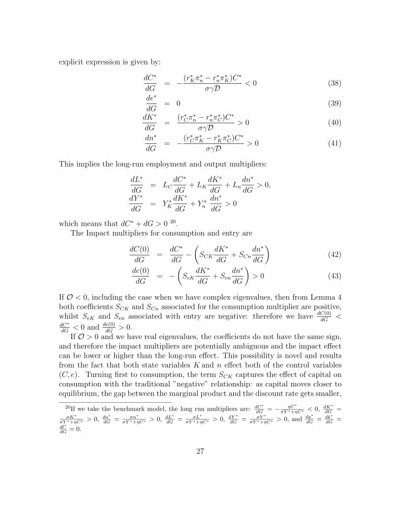
which means that dC∗ + dG > 0 20.The Impact multipliers for consumption and entry are

dC(0)

dG=

dC∗

dG−(SCK

dK∗

dG+ SCn

dn∗

dG

)(42)

de(0)

dG= −

(SeK

dK∗

dG+ Sen

dn∗

dG

)> 0 (43)

If O < 0, including the case when we have complex eigenvalues, then from Lemma 4both coefficients SCK and SCn associated for the consumption multiplier are positive,whilst SeK and Sen associated with entry are negative: therefore we have dC(0)

dG<

dC∗

dG< 0 and de(0)

dG> 0.

If O > 0 and we have real eigenvalues, the coefficients do not have the same sign,and therefore the impact multipliers are potentially ambiguous and the impact effectcan be lower or higher than the long-run effect. This possibility is novel and resultsfrom the fact that both state variables K and n effect both of the control variables(C, e). Turning first to consumption, the term SCK captures the effect of capital onconsumption with the traditional ”negative” relationship: as capital moves closer toequilibrium, the gap between the marginal product and the discount rate gets smaller,

20If we take the benchmark model, the long run multipliers are: dC∗

dG = − ηC∗

σY ∗+ηC∗ < 0, dK∗

dG =σK∗

σY ∗+ηC∗ > 0, dn∗

dG = σn∗

σY ∗+ηC∗ > 0, dL∗

dG = σL∗

σY ∗+ηC∗ > 0, dY ∗

dG = σY ∗

σY ∗+ηC∗ > 0, and dy∗

dG = dk∗

dG =dl∗

dG = 0.

27

hence consumption continues to grow but at a slower rate, implying the monotonictrajectory of consumption rising alongside capital accumulation. However, the termSCn captures the effect of entry on the Euler equation for consumption. More firmscan counteract the increase in capital leading to a non-monotonic trajectory in themarginal product of capital (which depends on capital per firm k, not aggregatecapital) and hence also non-monotonicity in consumption. This leads to an ambigu-ous relation between initial consumption and its long-run value if the entry flow islarge initially so that capital per firm decreases and the marginal product of capi-tal increases. This sort of consumption undershooting response is impossible in theclassic Ramsey model where the marginal product depends only on the aggregatecapital stock and the impact response of consumption always overshoots the long-runresponse21.

6.2 Hump-shaped responses.

The short run dynamics is similar to the one generated by equation (30). The exis-tence of non-monotonic adjustment trajectories depend both on the parameters andon the type magnitude of the shock. If we take the after-shock levels of capital andnumber of firms as K∗ and n∗ and the pre-shock values as initial values, we cancompare the variation with the expressions for the expressions in Proposition 4.

[ Figure 4 here]

Proposition 5. Assume there is a permanent fiscal policy shock. If ∆ > 0 then theadjustment for K is always monotonic and the adjustment for n is hump-shaped forcase R3 and monotonic for cases R1 and R2. If ∆ < 0 the adjustment is oscillatoryfor both variables.

In Figure 3 we have already shown the four possible cases of short-run dynamics.We see that there is a monotonic adjustment of both (K,n) for cases R1 and R2, anda non-monotonic adjustment for cases C and R3. Since we are looking at the responseof changes to fiscal policy the initial position will lie on the dG line: hence. Figure 4superposes the dG line. We can see that if we started from an initial steady-state andit is peturbed by dG, the initial steady-state will belong to to sets Wn and En of thenew steady-state. and only the number of firms can adjust non-monotonously. Thisis an ”initial condition effect”, and would not hold if we were to consider technologyshocks. Whilst for all cases R1,R2, R3 and C capital will adjust monotonically inresponse to fiscal policy, capital stock per firm may be non-monotonic in all cases. If

21In the classic Ramsey model in (C,K), the saddlepath is upwards sloping so (C,K) movetogether with an endogenous labour supply.

28

we turn to output, in case R1 the Y = 0 isocline is downward sloping, which impliesthat output always responds monotonically to fiscal policy. However, the Y = 0isocline is upward sloping and flatter than the dG line in the other cases: output willalways be non-monotonic in cases R3 and C and may be in case R2.

Phase diagram R3 is depicted in Figure 3, SW panel. In this case both curves Es1

and Es2 are negatively sloped. Since Es

1 < 0 there is a negative co-movement betweenthe two state variables (K,n) as we approach the steady-state. Furthermore, sincedG lies in between the K = 0 and n = 0 isoclines, the initial co-movement is positive.The trajectories also cross the n = 0 isocline, indicating an overshooting hump shapefor n. The other point to note is that the Y = 0 line is positively sloped. This meansthat any trajectory originating from the dG line must pass through Y = 0: henceoutput must have a hump shape response. Phase diagram C, associated with theexistence of complex eigenvalues, is depicted in Figure 4, SE panel and is qualitativelysimilar to R3: the reason for this is that all trajectories starting on dG must start offwith positive co-movement (in order to get negative co-movement initially, we wouldneed to start from a point the ”other side” of the K = 0 isocline which is off the dGline).

Phase diagram R1 is depicted in Figure 4, NW panel. Its main features are thefollowing. First, asymptotically the aggregate capital stock and the number of firmsare positively related in the neighborhood of the steady state, and will be tangentasymptotically to Es

1. Since the initial position lies on dG, the initial co-movementwill also be positive. Since the trajectory cannot cross any of the n,= K = Y = 0lines, along the trajectory of n,K, and Y all move together (this is the same as theexogenous labour case Brito and Dixon (2009)). Phase diagram R2 is depicted inFigure 4, NE panel. It shares some similar properties with the phase diagram R1, inparticular, the positive co-movement of the two state variables in the neighborhoodof the steady state. However, it differs in that trajectories originating from dG maycross the Y = 0 line. Hence there may be a hump shaped response of output to fiscalpolicy.

Another way of looking at the dynamics is through the impulse-response functionsfor the main variables to a fiscal shock in this model, (C, Y,K,L, n, e, k, I) wherek = K/n is capital per firm and I is investment in new firms and capital (see Figures5 to 8). The impulse-response functions for all cases show that capital-per firm kis non-monotonic. However, we also observe that whilst consumption and capitalin all cases follow monotonic trajectories (in this benchmark case), this is not so foroutput Y and employment L. In the case of phase diagram C, where there are twocomplex eigenvalues and n adjusts non-monotonically, we can see that both outputand employment have a hump-shaped response function: output and employment”jump” up, but continue upwards for a time overshooting the long-run effect, peakingand then converging to the new steady-state.

29

[ Figures 5 to 8 here]

Whilst we have not found an example of a non-monotonic trajectory for con-sumption in the benchmark model, we can determine what it would look like if itwere to happen. Since the marginal product of capital will fall as we approach closeto the steady-state, we know that consumption and capital will then have a positiveco-movement. In the classical Ramsey model, with overshooting, the positive co-movement occurs all along the path. However, if there is undershooting on impact,then consumption will at first fall to below (in the case of a fiscal expansion) the newsteady-state, so that it can then increase with capital. There will thus be an initialphase of negative co-movement resulting in a hump shape.

7 Conclusion

In this paper we have analyzed Ricardian fiscal policy in the context of the classicRamsey model extended to include an endogenous labour supply and a real timeentry and exit process. Both of these extensions have been done on their own:entry was developed in Brito and Dixon (2009) and an endogenous labour supply in(Turnovsky, 1995, ch.9). We find that with both extensions together we are able toobtain a much richer set of possible dynamic responses to fiscal policy. Whilst thelong-run dynamics are similar to standard models, the short-run can be very different.The dynamics allows for complex eigenvalues so that both state variables (capital andthe number of firms) can be non-monotonic.

However, in the analysis of fiscal policy there is an ”initial condition” effect thatimplies that only the number of firms will be non-monotonic as we move from theinitial steady-state to the new one. Whilst the response of capital to fiscal policywill be monotonic, we find that there can be a hump shaped response of output in awide range of cases. This is analyzed in terms of a phase diagram in the state-spaceof capital and the number of firms, where we are able to define the isocline for output(the combinations of capital and the number of firms at which the time derivative ofoutput is zero). We are able to show that in certain well defined cases the trajectoryof the economy in response to a fiscal shock will pass through this isocline and thusexhibit a hump shaped response.

Much of macroeconomics today is thought of in terms of calibrated or estimatednumerical models. Whilst theory has its limitations in being limited to sheddinglight on relatively simple models, theoretical models allow us to understand the gen-eral mechanisms underlying macroeconomic relationships in a way that numericalsimulation cannot. We have extended the standard Ramsey model by introducinga real time model of entry. Whilst the analysis is complex and four dimensional,

30

we are able to interpret the results in terms of two dimensional phase diagrams withrelatively clear economic interpretation.

The profile of the trajectories generated by a dynamic model is determined bythe number of independent dynamic mechanisms, which can be measured by thedimension of the stable manifold. Sometimes calibrated DSGE models are largein terms of the dimension but they are not large in terms of the dimension of thestable manifold. An analytical approach has the advantage of rendering the dynamicmechanisms transparent. In this paper we have learned that in order to have hump-shaped trajectories the dimension of the stable manifold should be two and that thetwo dynamic driving forces are the decreasing marginal productivity of capital inproduction and the decreasing marginal profit on entry.

References

Baxter, M. and King, R. G. (1993). Fiscal policy in general equilibrium. The AmericanEconomic Review, 83(3):pp. 315–334.

Brito, P. and Dixon, H. (2009). Entry and the accumulation of capital: a two state-variable extension to the Ramsey model. International Journal of Economic The-ory, 5(4):333–357.

Brock, W. A. and Turnovsky, S. J. (1981). The analysis of macroeconomic policiesin perfect foresight equilibrium. Internationl Economic Review, 22(1):179–209.

Burnside, C., Eichenbaum, M., and Fisher, J. D. M. (2004). Fiscal shocks and theirconsequences. Journal of Economic Theory, 115(1):89 – 117.

Cass, D. (1965). Optimum growth in an aggregative model of capital accumulation.Review of Economic Studies, 32:233–40.

Christiano, L. J., Eichenbaum, M., and Evans, C. L. (2005). Nominal rigidities andthe dynamic effects of a shock to monetary policy. Journal of Political Economy,13(1):1–45.

Costa, L. and Dixon, H. D. (2011). Fiscal policy under imperfect competition withflexible prices: An overview and survey. Economics: The Open-Access, Open-Assessment E-Journal, 5(3).

Das, S. and Das, S. (1996). Dynamics of entry and exit of firms in the presence of entryadjustment costs. International Journal of Industrial Organization, 15:217–241.

31

Datta, B. and Dixon, H. (2002). Technological change, entry, and stock marketdynamics: an analysis of transition in a monopolistic economy. American EconomicReview, 92(2):231–235.

Dixon, H. (1987). A simple model of imperfect competition with Walrasian features.Oxford Economic Papers, 39(1):pp. 134–160.

Jaimovich, N. and Floetotto, M. (2008). Firm dynamics, markup variations, and thebusiness cycle. Journal of Monetary Economics, 55:1238–1252.

Koopmans, T. (1965). On the concept of optimal economic growth. In The Econo-metric Approach to Development Planning. Pontificiae Acad. Sci., North-Holland.

Linneman, L. (2001). The price index effect, entry, and endogenous markups in amacroeconomic model of monopolistic competition. Journal of Macroeconomics,23:441–458.

Mankiw, N. G. (1988). Imperfect competition and the Keynesian cross. EconomicsLetters, 26(1):7 – 13.

Melitz, M. J. (2003). The impact of trade on intra-industry reallocations and aggre-gate industry productivity. Econometrica, 71(6):1695–1725.

Mountford, A. and Uhlig, H. (2009). What are the effects of fiscal policy shocks?Journal of Applied Econometrics, 24(6):960–992.

Ramsey, F. P. (1928). A mathematical theory of saving. Economic Journal,38(Dec):543–59.

Smets, F. and Wouters, R. (2003). An estimated dynamic stochastic general equi-librium model of the Euro area. Journal of the European Economic Association,1(5):1123–1175.

Startz, R. (1989). Monopolistic competition as a foundation for Keynesian macroe-conomic models. The Quarterly Journal of Economics, 104(4):pp. 737–752.

Takayama, A. (1994). Analytical Methods in Economics. Harvester Wheatsheaf.

Turnovsky, S. (1990). The effects of taxes and dividend policy on capital accumulationand macroeconomic behaviour. Jounal of Economic Dynamics and Control, 14(3-4):491–521.

Turnovsky, S. (1995). Methods of Macroeconomic Dynamics. MIT Press.

32

Turnovsky, S. and Sen, P. (1991). Fiscal policy, capital accumulation, and debt in anopen economy. Oxford Economic Papers, 43(1):1–24.

Woodford, M. (2011). Simple analytics of the government expenditure multiplier.American Economic Journal: Macroeconomics, 3(January):1–35.

Yang, X. and Heijdra, B. J. (1993). Monopolistic competition and optimum productdiversity: comment. The American Economic Review, 83(1):295–301.

33

A Appendix: proofs and auxiliary results

Partial derivatives of function (2) The first partial derivetione of function (2)are

YK = AFk

(K

n,L

n

), YL = AFl

(K

n,L

n

), Yn = (1− ν)AF

(K

n,L

n

)− φ

where YK = ∂Y/∂K, etc. The last equation results from the application of Euler’sLemma. The second partial derivatives are:

YKK =AFkkn

< 0, YKL = YLK =AFkln

> 0, YLL =AFlln

< 0

and

YnK = YKn = (1−ν)AFkn

> 0, YnL = YLn = (1−ν)AFln

> 0, Ynn = −ν(1− ν)AF

n< 0.

Partial derivatives of function (7) Assuming that UCL 6= 0 the optimal laboursupply function has partial derivatives:

LC = − YLUCCUCYLL + ULL

< 0

LK = − YLKUCUCYLL + ULL

> 0

Ln = − YLnUCUCYLL + ULL

> 0.

Partial derivations of functions (8), (9) and (10) The partial derivatives forthe optimal rate of return are

rC = YKLLC < 0

rK = YKK + YKLLK =(YKKYLL − YKLYLK)UC + YKKULL

UCYLL + ULL< 0

rn = YKn + YKLLn > 0

we use the following facts (resulting from the concavity of the production function)

YKKYLL − YKLYLK =

(A

n

)2

(FkkFll − F 2kl) > 0

34

The partial derivatives for the optimal profits are

πC = YnLLC < 0

πK = YnK + YnLLK > 0

πn = Ynn + YnLLn =(YnnYLL − YnLYLn)UC + YnnULL

UCYLL + ULL< 0

we use the following facts (resulting from the concavity and rhe homogeneity of degreeν of the production function)

YnnYLL−YnLYLn =

(A

n

)2K

n((ν−1)FkFll−(ν−1)FlFlk) =

(AK

n2

)2

(FkkFll−F 2kl) > 0

The partial derivatives for the optimal output are

YC = YLLC = wLC < 0

YK = YK + YLLK = r + wLK > 0

Yn = Yn + YLLn = π + wLn

which is ambiguous, but Yn > 0 at the steady state because π∗ = 0.

Propositions 1 and 2: auxiliary results and proofs

Lemma 1. Let D = det (J), T = M2 − ρ2, where M2 is the sum of the principalminors of order 2 of J Then, the eigenvalues of Jacobian J , are

λs,u1 =ρ

2∓[(ρ

2

)2− T

2−∆

12

] 12

, λs,u2 =ρ

2∓[(ρ

2

)2− T

2+ ∆

12

] 12

(44)

where the discriminant is ∆ ≡(T2

)2 −D.

Proof. The characteristic polynomial for a four dimensional system of ODEs is:

c(λ) = λ4 −M1λ3 +M2λ

2 −M3λ+M4

where Mj is the sum of the principal minors of order j = 1, . . . , 4. In infinite horizonoptimal control problems with two state variables the following constraints on thevalue of the sums of the principal minors hold: M2 = 2ρ, which is the trace, andM3 = ρ(M2 − ρ2). Therefore, there are only two independent coefficients involvingthe sums of the principal minors of even order: T ≡M2 − ρ2 and D ≡M4 = det(J).Then the characteristic polynomial can be written as

c(λ) =(ρ

2

)4 [ω2 +

((ρ2

)−2T − 2

)ω +

((ρ2

)−4M4 −

(ρ2

)−2T + 1

)],

35

where ω ≡(λ− ρ

2

)2 (ρ2

)−2. Then we get the eigenvalues as

(λ− ρ

2

)s,u1,2

= ∓[(

ρ2

)ω1,2

] 12 .

Then, by solving the polynomial equation c(λ) = 0, we get the eigenvalues in equation(44).

Lemma 2. If the discriminant is non-negative, ∆ ≥ 0, then the four eigenvalues arereal and verify

λs2 ≤ λs1 < 0 < λu1 ≤ λu2 .

If the discriminant is negative, ∆ < 0, then there are two pairs of complex conjugateeigenvalues

λs1 = θs + ϑi, λs2 = θs − ϑi, λu1 = θu − ϑi, λu2 = θu + ϑi

where i2 = −1, and θs < 0 < θu:

θs,u =ρ

2∓(

1

2

)1/2{[(ρ

2

)4−(ρ

2

)2T +D

]1/2+(ρ

2

)2− T

2

}1/2

and

ϑ =

(1

2

)1/2{[(ρ

2

)4−(ρ

2

)2T +D

]1/2−(ρ

2

)2+T2

}1/2

> 0.

Furthermore, the following relationships hold:

1. λsi + λui = ρ > 0 (if they are complex we have αs + αu = ρ);

2. λs1λu1 = l1 and λs2λ

u2 = l2,

l1 =

{T2

+ ∆12 , if ∆ ≥ 0

T2

+ (|∆|) 12 i, if ∆ < 0

, l2 =

{T2−∆

12 , if ∆ ≥ 0

T2− (|∆|) 1

2 i, if ∆ < 0

verify l2 ≤ l1 < 0 are real if ∆ ≥ 0 and are complex conjugate with a negativereal part, if ∆ < 0

3. l1 + l2 = T < 0 and l1l2 = D > 0 are real for any type of eigenvalue, real orcomplex.

Proof. Proof of Lemma 2 The first part of the Lemma is obvious from Lemma 1.When ∆ < 0 we use the fact that given the complex number y = a + bi it is knownthat

√y =√a+ bi = 1/2

{√r + a+ sign(b)

√r − ai

}where r ≡

√a2 + b2. The rest

of the proof is obvious.

36

Proof. Proof of Proposition 1 We start by proving that the conditions of Lemma1 on the sums of the principal minors hold.

First, as C∗

σYKLLC + YLLK = 0 then

C∗r∗Cσ

+ Y ∗K = ρ which implies that the trace

is M1 = ρ +C∗r∗Cσ

+ Y ∗K = 2ρ. Second, the sum of the principal minors of order twoand three are

M2 = ρ

(C∗r∗Cσ

+ Y ∗K

)+C∗

σ(r∗CY

∗K − r∗K(Y ∗C − 1)) +

π∗nγ

and

M3 = ρ(M2 − ρ2)−1

γ

(C∗

σr∗nπ

∗C + π∗KY

∗n

)But as C∗

σr∗nπ

∗C + π∗KY

∗n = 0 then M3 = ρ(M2 − ρ2). Then, we can use Lemma 1 to

determine the eigenvalues, noting that

T ≡M2 − ρ2 =C∗

σ(r∗CY

∗K − r∗KY ∗C) +

C∗r∗Kσ

+π∗nγ

(45)

and

D ≡M4 =C∗

σγ[(1− Y ∗C)(π∗nr

∗K − π∗Kr∗n) + Y ∗K(π∗nr

∗C − π∗Cr∗n)− Y ∗n (π∗Kr

∗C − π∗Cr∗K)]

(46)In order to obtain the dimension of the stable manifold, we have to determine the

signs of T and D. From the signs of the partial derivatives, r∗K < 0, π∗n < 0 and asr∗CY

∗K − r∗KY ∗C = LC(YLKYK − YKKYL) < 0 then T < 0. As

D =C∗

σγ

(L∗

n∗

)(1

UCYLL + ULL

)(AFYLUCC + ULL

L∗

n∗

)(YKKYLL − YKLYLK) > 0

(47)From the fundamental theorem of algebra (i.e., on the relationship between the eigen-values and the coefficients of the characteristic polynomial) it is easy to see that thereare two eigenvalues with negative real parts (and always two eigenvalues with positivereal parts): D > 0 implies that there are no zero eigenvalues and that the number ofeigenvalues with negative real part is even; but as M1 > 0 they should be reduced tozero or two; and, finally as M3 = ρT < 0 then we should have one pair of negativeeigenvalues (M2 is ambiguous, in general).

Next, we apply the results in Lemma 2. For finding the conditions under whichthose three cases can occur let z ≡ 1/γ. The ”inner” discriminant can be written asa quadratic function of z:

∆(z) =

(π∗n2

)2[z2 + 2

(2O − π∗nQ

(π∗n)2

)z +

(Qπ∗n

)2]. (48)

37

Then ∆(z) = 0 if and only if δ(z) = z2 + a1z + a0 = 0, such that z > 0, where

a1 ≡ 2(

2O−π∗nQ(π∗n)

2

)and a0 ≡

(Qπ∗n

)2. The sign of a1 is ambiguous but a0 > 0.

Function δ(z) has a minimum for z > 0 such that δ′(z) = 0. If δ(z) = 0 then

if z = z then there will be multiple real eigenvalues and if z 6= z there will be realdistinct eigenvalues. If δ(z) < 0 this means that the polynomial has two roots, z1 andz2 such that z1 > z2 > 0. Then there are related values for γ, γ1 < γ2. This impliesthat ∆(z) < 0 for z1 > z > z2 and the eigenvalues, λji for j = s, u and i = 1, 2 will becomplex conjugate.

Therefore, we have only to investigate if there are any positive real roots for thepolynomial equation δ(z) = 0. Its roots are

z1 = (π∗n)−2{π∗nQ− 2O + 2 [O(O − π∗nQ)]

12

},

z2 = (π∗n)2{π∗nQ− 2O − 2 [O(O − π∗nQ)]

12

}.

Observe that as a0 > 0 then the two roots, z1, z2, have the same sign, but may bereal or complex.

Let ∆z ≡ O(O − π∗nQ). Three cases may occur:(a) ∆z = 0 if O = 0 or O = π∗nQ > 0. In each of those cases there is only one

multiple solution for δ(z) = 0. In the first case, we get z = z = Q/π∗n > 0, given inequation (33). In the second case we get z = −Q/π∗n < 0 which does not belong tothe domain of z.

(b) ∆z < 0 if O−π∗nQ < 0 < O (another formally possible case where O−π∗nQ >0 > O is not admissible because π∗nQ > 0). In this case z1 and z2 are complexconjugate and therefore do not belong to the domain of z.

(c) ∆z > 0 if O < 0, implying that O − π∗nQ < 0, or if O > O − π∗nQ > 0. In thefirst case, as a1 is positive because πnQ− 2O > 0, and as a0 is positive, then the tworoots for δ(z) = 0 are real and positive. In the second case, as π∗nQ−O < −O < 0then a1 < 0 and the two roots are real but negative, and, therefore do not belong tothe domain of z.

Summing up, O < 0 is a necessary condition for ∆(z) < 0 because z > 0. Thiscase occurs if and only if z1 < z < z2. In all the other cases the eigenvalues are real.

The rest of the proof follows from Lemma 2.

Lemma 3. If there is no multiplicity then is the eigenvector associated to eigenvalueλsj, j = 1, 2 of matrix J is

V sj = (vs1,j, λ

sj , v

s3,j, 1)>, j = 1, 2 (49)

38

where

vs1,1 ≡C∗

σ(r∗KY

∗n − r∗nY ∗K + r∗nλ

s1)

l2 − π∗nγ

, vs3,1 ≡C∗

σ((Y ∗C − 1)r∗n − Y ∗n r∗C) + Y ∗n λ

s1

l2 − π∗nγ

(50)

vs1,2 ≡C∗

σ(r∗KY

∗n − r∗nY ∗K + r∗nλ

s2)

l1 − π∗nγ

, vs3,2 ≡C∗

σ((Y ∗C − 1)r∗n − Y ∗n r∗C) + Y ∗n λ

s2

l1 − π∗nγ

(51)

Proof. Eigenvector V ij is obtained as the non-zero solution of the homogeneous system

(J − λijI4)V ij = 0,

V ij =

[C∗

σ

(r∗KY

∗n − r∗n(Y ∗K − λij)

)(C∗

σ− λij)(r∗K − λij)− C∗

σr∗K(Y ∗C − 1)

, λij,C∗

σr∗n(Y ∗C − 1)− Y ∗n

(C∗

σr∗C − λij

)(C∗

σr∗C − λij)(r∗K − λij)− C∗

σr∗K(Y ∗C − 1)

, 1

],

for i = s, u and j = 1, 2. But (C∗

σ−λij)(r∗K −λij)− C∗

σr∗K(Y ∗C − 1) = (λij)

2−λij(C∗

σr∗C +

Y ∗K) + C∗

σr∗CY

∗K − C∗

σr∗K(Y ∗C − 1) = λij(λ

ij − ρ) + T − π∗n

γ= −li + l1 + l2 − π∗n

γ, because

T = l1+l2 and λsi+λui = ρ. Then, for V s

1 and V u1 the denominator becomes l2− π∗n

γand

for V s2 and V u

2 the denominator becomes l1 − π∗nγ

. Then equation (49) results. If the

eigenvalues are complex, then l1 = λs1λu1 = (θs+ϑi)(θu−ϑi) = θsθu+ϑ2−ϑ(θu−θs)i =

T /2 + |∆|1/2i and l2 is its complex conjugate l2 = T /2− |∆|1/2i.

Proof. Proof of Proposition 2We start with the determination of the slopes of the (K,n) projections of the

eigenspaces in space (K,n), for the ∆ > 0 case: dndK

∣∣Es

1= 1/vs3,1 and dn

dK

∣∣Es

2=

1/vs3,2. The numerators of the vs1,i and vs3,i, for i = 1, 2, in equations (50)-(51),are negative. In order to determine the sign of the denominators observe that l1 −π∗nγ

= 12

(Q− π∗n

γ+ ∆

12

)and l2 − π∗n

γ= 1

2

(Q− π∗n

γ−∆

12

)where Q < 0, π∗n < 0, and

∆ =(Q− π∗n

γ

)2+ 4O

γ. As the sign of O is ambiguous then the signs of ∆, l1 − π∗n

γ

and l2 − π∗nγ

are also ambiguous. However, if we want to guarantee that ∆ > 0 we

readily conclude that, three cases may occur: (1) if O > 0 then the second memberis larger in absolute value and therefore l1 − π∗n

γ> 0 > l2 − π∗n

γ. To see this note that

we have

[(Q− π∗n

γ

)2+ 4O

γ

] 12

>∣∣∣Q− π∗n

γ

∣∣∣ ≥ Q− π∗nγ

. Then vs1,1 > 0 and vs3,1 > 0, and

vs1,2 < 0 and vs3,2 < 0. If O < 0 and ∆ > 0, the first member is larger in absolutevalue and therefore the sign of the denominators are equal and are the same as the

39

sign of Q − π∗nγ

. Therefore, we have two cases: (2) if O < 0, and Q − π∗nγ< 0, then

vs1,1 > 0, vs3,1 > 0, vs1,2 > 0 and vs3,2 > 0; or (3) if O < 0, and Q− π∗nγ> 0 then vs1,1 < 0,

vs3,1 < 0, vs1,2 < 0 and vs3,2 < 0.

Then, the signs of dndK

∣∣Es

1and dn

dK

∣∣Es

2are clear. In addition, we have a relationship

between those slopes

dn

dK

∣∣∣∣Es

1

− dn

dK

∣∣∣∣Es

2

=C∗

σr∗n(l1 − l2) + Y ∗n (λs2 − λs1)(Q− λu1λu2)

(C∗

σr∗n + Y ∗n λ

u1)(C

∗

σr∗n + Y ∗n λ

u2)

> 0

for any case of the three previous cases. Then: 1. If O > 0 then dndK

∣∣Es

1> 0 and

dndK

∣∣Es

2< 0; 2. If O < 0 and π∗n > γQ then dn

dK

∣∣Es

1> dn

dK

∣∣Es

2> 0; 3. If O < 0 and

π∗n < γQ then 0 > dndK

∣∣Es

1> dn

dK

∣∣Es

2.

Proposition 3: auxiliary results and proof

Lemma 4. (Local projection of (C, e) on the stable eigenspace). The linear spacewhich is tangent to the stable manifold is given by

Es ≡{

(C, e,K, n) : (C − C∗, e)> = S(K −K∗, n− n∗)>}

where

SCK =C∗

σ(r∗KY

∗n − r∗nY ∗K)(l1 − l2) + C∗

σr∗n(λs1 − λs2)(Q− λs1λs2)

C∗

σr∗n(l2 − l1) + Y ∗n (λu2 − λu1)(Q− λu1λu2)

> 0 (52)

SCn =C∗

σr∗n(λs1 − λs2)O/γ

π∗Kγ

[C∗

σr∗n(l2 − l1) + Y ∗n (λu2 − λu1)(Q− λu1λu2)

] (53)

SeK =(λs2 − λs1)O/γ

C∗

σr∗n(l2 − l1) + Y ∗n (λu2 − λu1)(Q− λu1λu2)

(54)

Sen =

C∗

σ((Y ∗C − 1)r∗n − Y ∗n r∗C) (λs2 − λs1)(λs1λs2 −

π∗nγ

) + Y ∗n λs1λ

s2(l1 − l2)

C∗

σr∗n(l2 − l1) + Y ∗n (λu2 − λu1)(Q− λu1λu2)

< 0(55)

If O > 0 then SCn < 0, SeK > 0 and SCK/SCn < SeK/Sen < 0. If O < 0 thenSCn > 0, SeK < 0 and SCK/SCn > SeK/Sen > 0.

Proof. Following the same method as in Brito and Dixon (2009) we prove this bysolving the last two equations of (30) for the two constants, zs1 and zs2 as

zs1 =

(K(t)−K∗ − vs3,2(n(t)− n∗)

vs3,1 − vs3,2

)e−λ

s1t

zs2 =

(−(K(t)−K∗) + vs3,1(n(t)− n∗)vs3,1 − vs3,2

)e−λ

s2t

40

and substitute in the solutions for C and e in equation (30) to get (C(t)−C∗, e(t)−e∗)> = S(K(t)−K∗, n(t)− n∗)> where

S ≡ 1

vs3,1 − vs3,2

(vs1,1 − vs1,2 vs1,2v

s3,1 − vs3,2vs1,1

λs1 − λs2 λs2vs3,1 − λs1vs3,2

).

After some algebra we get equations (52) to (55). We already know, from the concav-ity properties of the production and utility functions, that r∗n > 0, Y ∗n > 0, π∗K > 0and π∗n < 0. Also r∗KY

∗n − r∗nY ∗K < 0 and (Y ∗C − 1)r∗n − Y ∗n r∗C < 0 because

Y ∗Cr∗n − Y ∗n r∗C = LC (YL(YKn + YKLLn)− YKLYLLn) = LCYLYKn < 0.

If the eigenvalues are real then all the denominators are negative because l2− l1 < 0,Q < 0, and because of the relationships between the eigenvalues, λs2 < λs1 < 0 < λu1 <λu2 . The numerator of SCK is negative and the numerator of Sen is positive. At last,we see that the signs of the numerators of SCn and SeK are symmetric. Note that, ifO > 0 then l2−Q < 0 < l1−Q and if O < 0 then the signs of l2−Q and l1−Q arethe same. On the other hand (l1 −Q)(l2 −Q) = −O/γ. Then the sign of SeK is thesame as O and is the symmetric of SCn.

If the eigenvalues are complex we can prove that all the coefficients are of type(ai)/(bi) = a/b and they are also real. The denominator is a complex number withzero real part and a negative coefficient to the complex part l2 − l1 = −2|∆|1/2i and(λu2 − λu1)(Q − λu1λ

u2) = (Q − (θu)

2 − ϑ2)2ϑi have both negative coefficients. Thenumerator of SCK is also complex number with negative coefficient to the complexpart as (λs1 − λs2)(Q − λs1λs2) = (Q − (θs)

2 − ϑ2)2ϑi. If we apply the same methodto the other coefficients we observe that the numerator of all the other coefficientsare complex numbers with zero real part and SCn has a negative coefficient to thecomplex part and SeK and Sen have positive coefficients to the complex part.

At last, as

det (S) =λs2v

s1,1 − λs1vs1,2vs3,1 − vs3,2

=

=

C∗

σ(r∗KY

∗n − r∗nY ∗K)((λs1 − λs2)

π∗nγ

+ λs2λs1(λ

u1 − λu2)) + r∗nλ

s2λ

s1(l1 − l2)

C∗

σr∗n(l2 − l1) + Y ∗n (λu2 − λu1)(Q− λu1λu2

,

which is negative because

r∗KY∗n − r∗nY ∗K = Ln(YKKYL − YKLYK)− YKn(YK + YLLK) < 0,

then det (S) = SCKSen − SCnSeK < 0.

41

Lemma 5. (Slopes of the isoclines in the projected space) The isoclines and theirrelative slopes in the projected space (K,n) verify:

1. if O > 0 then dndK

∣∣K=0

> dndK

∣∣C=0

> dndK

∣∣e=0

> dndK

∣∣n=0

> 0;

2. if O < 0 then dndK

∣∣C=0

> dndK

∣∣K=0

> 0 > dndK

∣∣n=0

> dndK

∣∣e=0

.

Proof. The projection of the intersection of the isoclines with the stable eigenspaceover the space (K,n) have the following slopes:

dn

dK

∣∣∣∣K=0

= −Y∗K + (Y ∗C − 1)SCKY ∗n + (Y ∗C − 1)SCn

=λs2v

s3,2 − λs1vs3,1

vs3,1vs3,2(λ

s2 − λs1)

=

=C∗

σr∗n(λs1 − λs2)(Q− λs1λs2) + Y ∗nQ(l1 − l2)

(λs2 − λs1)(C∗

σr∗n + Y ∗n λ

u2)(C

∗

σr∗n + Y ∗n λ

u1)

> 0

dn

dK

∣∣∣∣C=0

= −r∗K + r∗CSCKr∗n + r∗CSCn

=λs2v

s1,2 − λs1vs1,1

λs2vs3,1v

s1,2 − λs1vs1,1vs3,2

=

=(r∗KY

∗n − r∗nY ∗K)(λs2 − λs1)(Q− λs1λs2) + r∗n((λs1)

2(l2 −Q)− (λs2)2(l1 −Q))

(r∗KY∗n − r∗nY ∗K)(λs1 − λs2)(C

∗

σr∗n) + r∗n(C

∗

σ((λs1)

2 − (λs2)2) + Y ∗n (λu2(λs1)

2 − λu1(λs2)2))

> 0

dn

dK

∣∣∣∣n=0

= −SCKSCn

=λs2 − λs1

λs2vs3,1 − vs3,2λs1

=

=(λs2 − λs1)(l1 −Q)(l2 −Q)

C?

σ((Y ?

C − 1)r?n − Y ?n r

?C)(λs2 − λs1)(λs1λs2 −

π?n

γ+ Y ?

n λs1λ

s2(l1 − l2)

and

dn

dK

∣∣∣∣e=0

= −π∗K + π∗CSCK − ργSeKπ∗n + π∗CSCn − ργSeK

=(λs2)

2 − (λs1)2

vs3,1(λs2)

2 − vs3,2(λs1)2=

=((λs1)

2 − (λs2)2)(l1 −Q)(l2 −Q)

C∗

σr?n((λs2)

2(l2 −Q)− (λs1)2(l1 −Q)) + Y ?

n (λu1(λs2)2(l2 −Q)− λu2(λs1)

2(l1 −Q))

have both the same sign as −(l1 −Q)(l2 −Q), then they have both the same sign ofO (see the proof of Lemma 4).

We can also determine the relationships between the projected isoclines. In somecases we can sign unambiguously:

dn

dK

∣∣∣∣K=0

− dn

dK

∣∣∣∣n=0

= −λs1λ

s2(v

s3,1 − vs3,2)2

(λs2 − λs1)vs3,1vs3,2(λs2vs3,1 − λs1vs3,2)> 0

42

because both the numerator and the denominator are negative because the sign ofvs3,1v

s3,2(λ

s2vs3,1 − λs1vs3,2) is the same as the sign of (l1 −Q)2(l2 −Q)2 > 0

dn

dK

∣∣∣∣C=0

− dn

dK

∣∣∣∣e=0

=λs1λ

s2(v

s3,1 − vs3,2)(λs1vs1,2 − λs2vs1,1)

(λs2vs1,2v

s3,1 − λs1vs1,1vs3,2)((λs2)2vs3,1 − (λs1)

2vs3,2)> 0

because both the numerator and the denominator are fractions with positive numer-ators and denominators equal to (l1 −Q)2(l2 −Q)2 > 0,

dn

dK

∣∣∣∣C=0

− dn

dK

∣∣∣∣n=0

=λs1λ

s2(v

s3,1 − vs3,2)(vs1,2 − vs1,1)

(λs2vs1,2v

s3,1 − λs1vs1,1vs3,2)(λs2vs3,1 − λs1vs3,2)

> 0

because both the numerator and the denominator are fractions with negative numer-ators and denominators equal to (l1 −Q)2(l2 −Q)2 > 0, and

dn

dK

∣∣∣∣K=0

− dn

dK

∣∣∣∣e=0

=λs1λ

s2(v

s3,1 − vs3,2)(λs2vs3,1 − λs1vs3,2)

vs3,1vs3,2(λ

s1 − λs2)((λs2)2vs3,1 − (λs1)

2vs3,2)> 0

because both the numerator and the denominator are fractions with negative numer-ators and denominators equal to (l1 −Q)2(l2 −Q)2 > 0.

Other relationships depend on the sign of O:

dn

dK

∣∣∣∣C=0

− dn

dK

∣∣∣∣K=0

=λs1λ

s2(v

s3,1 − vs3,2)(vs1,2vs3,1 − vs1,1vs3,2)

vs3,1vs3,2(λ

s2 − λs1)(λs2vs1,2vs3,1 − λs1vs1,1vs3,2)

anddn

dK

∣∣∣∣e=0

− dn

dK

∣∣∣∣n=0

=λs1λ

s2(λ

s2 − λs1)(vs3,1 − vs3,2)

(λs2vs3,1 − λs1vs3,2)((λs2)2vs3,1 − (λs1)

2vs3,2)

have both the sign of vs3,1 − vs3,2 which has the symmetric sign of (l1 −Q)(l2 −Q) =−O/γ then the difference in the slopes has the sign of O.

Lemma 6. (Phase diagrams over the projected space) If the eigenvalues are real,then the projections of the isoclines and of the eigenspaces over space (K,n) verifythe following relationships:

R1 if O > 0 then dndK

∣∣K=0

> dndK

∣∣C=0

> dndK

∣∣Es

1> dn

dK

∣∣e=0

> dndK

∣∣n=0

> 0 >dndK

∣∣Es

2,

43

R2 If O < 0, ∆ > 0 and π∗n > γQ then dndK

∣∣C=0

> dndK

∣∣K=0

> dndK

∣∣Es

1> dn

dK

∣∣Es

2>

0 > dndK

∣∣n=0

> dndK

∣∣e=0

;

R3 If O < 0, ∆ > 0 and π∗n < γQ then dndK

∣∣C=0

> dndK

∣∣K=0

> 0 > dndK

∣∣n=0

>dndK

∣∣e=0

> dndK

∣∣Es

1> dn

dK

∣∣Es

2.

Proof. The slopes of the eigenspaces in space (K,n) and the slopes of the projectionsin (K,n) of the intersections of the isoclines with the stable manifold projections werealready determined in Proposition 2, and 5. We use the same method as in the proofof the last result to get their relative position. This can only be done for the casein which the eigenvalues are real, because the eigenvectors associated to the complexeigenvalues are also complex: the slopes of the eigenvectors as regards the projectionsof the isoclines K = 0 and C = 0 can be unambiguously signed,

dn

dK

∣∣∣∣K=0

− dn

dK

∣∣∣∣Es

j

= λsjvs3,2 − vs3,1

vs3,1vs3,2(λ

s2 − λs1)

> 0, j = 1, 2

and

dn

dK

∣∣∣∣C=0

− dn

dK

∣∣∣∣Es

j

=λsjv

s1,j

vs3,j

(vs3,2 − vs3,1

λs2vs3,1v

s1,2 − λs1vs3,2vs1,1

)> 0, j = 1, 2;

however, they are ambiguous as regards the projections of the isoclines e = 0 andn = 0

dn

dK

∣∣∣∣e=0

− dn

dK

∣∣∣∣Es

j

=,(λsj)

2

vs3,j

(vs3,2 − vs3,1

(λs2)2vs3,1 − (λs1)

2vs3,2

)j = 1, 2

anddn

dK

∣∣∣∣n=0

− dn

dK

∣∣∣∣Es

j

=,λsjvs3,j

(vs3,2 − vs3,1

λs2vs3,1 − λs1vs3,2

)j = 1, 2

however, they have both the sign of lj − π∗/γ. Then: the differences as regards Es1

are negative for O > 0 or O < 0 and π∗ > γQ (i.e., cases R1 and R2) and are positivefor O < 0 and π∗ < γQ (i.e., case R3 ); and he differences as regards Es

2 are positivefor O > 0 or O < 0 and π∗ < γQ (i.e., cases R1 and R3) and are negative for O < 0and π∗ > γQ (i.e., case R2 ).

Proof. Proof of Proposition 3 Consider equation (30) and the that the initial pointis not the steady state (K(0), n(0)) 6= (K∗, n∗). First, if the eigenvalues are complexthen the transition dynamics is oscillatory and convergent. As the the coefficient of

44

the complex part is positive ϑ > 0 then the trajectories rotate clockwise (see proof ofLemma 2). Next we deal with the case in which the eigenvalues are real.

First, consider the equation for K: K(t)−K∗ = zs1vs3,1e

λs1t + zs2vs3,2e

λs2t. As eλs1t >

eλs2t ≥ 0 if 0 ≤ t ≤ ∞ then the trajectories for K(t) are monotonic if sign(zs1v

s3,1) =

sign(zs2vs3,2) and they are non-monotonic if sign(zs1v

s3,1) 6= sign(zs2v

s3,2). There are four

types of trajectories: trajectory type I if K(0)−K∗ > 0 and K(t)−K∗ is decreasingtowards zero (K(∞) = K∗); trajectory type II if K(0)−K∗ is decreasing (it can bepositive, zero or negative) initially, reaches a level at time tK , K(tK) −K∗ < 0 andthen increases towards zero; trajectory type III if K(0) − K∗ < 0 and K(t) − K∗is increasing towards zero; and trajectory type IV if K(0)−K∗ is increasing (it canbe positive, zero or negative) initially, reaches a level at time tK , K(tK) − K∗ > 0and then decreases towards zero. Type II trajectory is a U hump-shaped trajectoryand type IV a IU hump-shaped trajectory. Hump-shaped trajectories only if tK ≡{t : d(K(t)−K∗)/dt = 0} > 0, while type II trajectories are convex at K(tK) andtype IV trajectories are concave at time K(tK). As

tK =1

λs1 − λs2ln

(−λs2z

s2vs3,2

λs1zs1vs3,1

)and

d2(K(t)−K∗)dt2

∣∣∣∣t=tK

= (λs1 − λs2)λs1zs1vs3,1eλs1tK

then, we have the following conditions for the four types of trajectories:

• trajectory I if λs1zs1vs3,1 + λs2z

s2vs3,2 < 0 and zs1v

s3,1 > 0;

• trajectory II if λs1zs1vs3,1 + λs2z

s2vs3,2 < 0 and zs1v

s3,1 < 0;

• trajectory III if λs1zs1vs3,1 + λs2z

s2vs3,2 > 0 and zs1v

s3,1 < 0;

• trajectory IV if λs1zs1vs3,1 + λs2z

s2vs3,2 > 0 and zs1v

s3,1 > 0.

In order to translate those conditions over a partition of the domain for variables(K,n), two facts are useful: first

λs1zs1vs3,1 + λs2z

s2vs3,2 =

(λs1vs3,1 − λs2vs3,2)(K(0)−K∗) + (λs2 − λs1)vs3,1vs3,2(n(0)− n∗)

vs3,1 − vs3,2= 0

if and only if (see proof of Lemma 5)

n(0)− n∗ =λs2v

s3,2 − λs1vs3,1

(λs2 − λs1)vs3,1vs3,2(K(0)−K∗) =

dn

dK

∣∣∣∣K=0

(K(0)−K∗)

45

that it (K(0), n(0)) are located along the projected isocline for K over space (K,n);second

zs1vs3,1 =

vs3,1((K(0)−K∗)− vs3,2(n(0)− n∗)

)vs3,1 − vs3,2

if and only if (see proof of Proposition 2)

n(0)− n∗ =1

vs3,2(K(0)−K∗) =

dn

dK

∣∣∣∣Es

2

(K(0)−K∗)

that is (K(0), n(0)) is located along the projected eigenspace Es2 over space (K,n).

Therefore, the projections of isocline K = 0 and of the eigenspace Es2 perform a

partition over the domain (K,n) which are associated to the four types of trajectoriesthat were mentioned. Using the previous results, and, in particular, the fact that ifO > 0 then vs3,1 − vs3,2 > 0 and vs3,1 > 0 and vs3,2 < 0 and if O < 0 then vs3,1 − vs3,2 < 0and sign(vs3,1) = sign(vs3,2), then we have:

• trajectory I if K(0) > K∗ and dndK

∣∣Es

2(K(0)−K∗) < n(0)−n∗ < dn

dK

∣∣K=0

(K(0)−K∗) ;

• trajectory II if n(0)− n∗ < min{

dndK

∣∣K=0

, dndK

∣∣Es

2

}(K(0)−K∗) ;

• trajectory III ifK(0) < K∗ and dndK

∣∣Es

2(K(0)−K∗) > n(0)−n∗ > dn

dK

∣∣K=0

(K(0)−K∗) ;

• trajectory IV if n(0)− n∗ > max{

dndK

∣∣K=0

, dndK

∣∣Es

2

}(K(0)−K∗).

Now, we consider the equation for n: n(t)−n∗ = zs1eλs1t+zs2e

λs2t. As eλs1t > eλ

s2t ≥ 0

if 0 ≤ t ≤ ∞ then the trajectories for n(t) are monotonic if sign(zs1) = sign(zs2) andthey are non-monotonic if sign(zs1) 6= sign(zs2). There are four types of trajectories:trajectory type I if n(0)−n∗ > 0 and n(t)−n∗ is decreasing towards zero (n(∞) = n∗);U hump-shaped trajectory of type II if n(0) − n∗ is decreasing (it can be positive,zero or negative) initially, reaches a level at time tn, n(tn)−n∗ < 0 and then increasestowards zero; trajectory type III if n(0)−n∗ < 0 and n(t)−n∗ is increasing towardszero; and IU hump-shaped of type IV if n(0) − n∗ is increasing (it can be positive,zero or negative) initially, reaches a level at time tn, n(tn)−n∗ > 0 and then decreasestowards zero. Hump-shaped trajectories only if tn ≡ {t : d(n(t)− n∗)/dt = 0} > 0,while type II trajectories are convex at n(tn) and type IV trajectories are concaveat time n(tn). As

tn =1

λs1 − λs2ln

(−λ

s2zs2

λs1zs1

)46

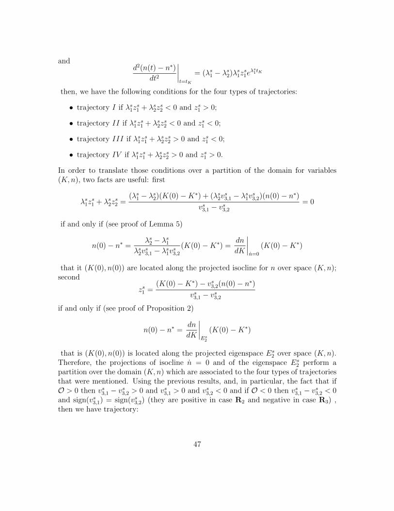
andd2(n(t)− n∗)

dt2

∣∣∣∣t=tK

= (λs1 − λs2)λs1zs1eλs1tK

then, we have the following conditions for the four types of trajectories:

• trajectory I if λs1zs1 + λs2z

s2 < 0 and zs1 > 0;

• trajectory II if λs1zs1 + λs2z

s2 < 0 and zs1 < 0;

• trajectory III if λs1zs1 + λs2z

s2 > 0 and zs1 < 0;

• trajectory IV if λs1zs1 + λs2z

s2 > 0 and zs1 > 0.

In order to translate those conditions over a partition of the domain for variables(K,n), two facts are useful: first

λs1zs1 + λs2z

s2 =

(λs1 − λs2)(K(0)−K∗) + (λs2vs3,1 − λs1vs3,2)(n(0)− n∗)

vs3,1 − vs3,2= 0

if and only if (see proof of Lemma 5)

n(0)− n∗ =λs2 − λs1

λs2vs3,1 − λs1vs3,2

(K(0)−K∗) =dn

dK

∣∣∣∣n=0

(K(0)−K∗)

that it (K(0), n(0)) are located along the projected isocline for n over space (K,n);second

zs1 =(K(0)−K∗)− vs3,2(n(0)− n∗)

vs3,1 − vs3,2if and only if (see proof of Proposition 2)

n(0)− n∗ =dn

dK

∣∣∣∣Es

2

(K(0)−K∗)

that is (K(0), n(0)) is located along the projected eigenspace Es2 over space (K,n).

Therefore, the projections of isocline n = 0 and of the eigenspace Es2 perform a

partition over the domain (K,n) which are associated to the four types of trajectoriesthat were mentioned. Using the previous results, and, in particular, the fact that ifO > 0 then vs3,1 − vs3,2 > 0 and vs3,1 > 0 and vs3,2 < 0 and if O < 0 then vs3,1 − vs3,2 < 0and sign(vs3,1) = sign(vs3,2) (they are positive in case R2 and negative in case R3) ,then we have trajectory:

47

• trajectory I if n(0) > n∗ and, if we have case R1 and dKdn

∣∣Es

2(n(0)−n∗) < K(0)−

K∗ < dKdn

∣∣n=0

(n(0)−n∗) or if we have cases R2 and R3 and dKdn

∣∣n=0

(n(0)−n∗) <K(0)−K∗ < dK

dn

∣∣Es

2(n(0)− n∗);

• trajectory II if we have case R1 and K(0)−K∗ < min{

dKdn

∣∣Es

2, dKdn

∣∣∣n=0

}(n(0)−

n∗) or if we have cases R2 and R3 andK(0)−K∗ > max{

dKdn

∣∣Es

2, dKdn

∣∣∣n=0

}(n(0)−

n∗);

• trajectory III if n(0) < n∗ and, if we have case R1 and dKdn

∣∣Es

2(n(0) − n∗) >

K(0)−K∗ > dKdn

∣∣n=0

(n(0)−n∗) or if we have cases R2 and R3 and dKdn

∣∣n=0

(n(0)−n∗) > K(0)−K∗ > dK

dn

∣∣Es

2(n(0)− n∗);

• trajectory IV if we have case R1 andK(0)−K∗ > max{

dKdn

∣∣Es

2, dKdn

∣∣∣n=0

}(n(0)−

n∗) or if we have cases R2 and R3 andK(0)−K∗ < min{

dKdn

∣∣Es

2, dKdn

∣∣∣n=0

}(n(0)−

n∗).

If we consider the definitions of sets NK , SK , Wn and En, then set NK is associatedto trajectories of type IV , set SK is associated to trajectories of type II, both forvariable K, and set Wn is associated to trajectories of type II for case R1 and oftype IV for cases R2 and R3 , and set En is associated to trajectories of type IVfor case R1 and of type II for cases R2 and R3, for variable n. Using the previousresults we also see that: (1) if we have case R1 the sets NK , SK , Wn and En are alldisjoint; (2) if we have case R2 then En ⊂ SK and Wn ⊂ NK ; and (3) if we havecase R3 then NK ⊂ En and SK ⊂Wn.

Propositions 4 and 5: proofs

Proof. Proof of Proposition 4 First, we linearise the system (12), (14), (15) and(16) around an initial steady state and introduce a variation in G, dG, to get thevariational system

X(t) = JdX(t) + JGdG

where X = (x1, x2, x3, x4)> ≡ (C, e,K, n)>, J is the Jacobian in equation (25) and

JG = (0, 0,−1, 0)>. Second, given the fact the steady state is hyperbolic, we get thelong run multipliers as dX∗/dG = −J−1JG. If we perform the matrix operation andobserve that det (J) = D > 0 then we get the expressions and the signs in equations(38)-(41). Third, to calculate the short-run multipliers we solve the linearised system,

48

along the stable manifold. We get, for the case in which the eigenvalues are real

dxi(t)

dG=dx∗idG−

vsi,1vs3,1 − vs3,2

(dK∗

dG− vs3,2

dn∗

dG

)eλ

s1t−

vsi,2vs3,1 − vs3,2

(−dK

∗

dG+ vs3,1

dn∗

dG

)eλ

s2t, i = 1, . . . , 4, (56)

and for the case in which the eigenvalues are complex conjugate

dxi(t)

dG=dx∗idG− 1

vs3,1 − vs3,2eθst{(

(vs1,1 − vsi,2)dK∗

dG− (vsi,1v

s3,2 − vsi,2vs3,1)

dn∗

dG

)cos (ϑt)+

+

((vsi,1 + vsi,2)

dK∗

dG− (vsi,1v

s3,2 + vsi,2v

s3,1)

dn∗

dG

)sin (ϑt)

}, i = 1, . . . , 4 (57)

If we evaluate the previous expressions at time t = 0, we get the same expressions forboth real and complex eigenvalues: dK(0)/dG = dn(0)/dG = 0 and equations (42)and (43) for dC(0)/dG and de(0)/dG. From Lemma 4, on the signs of the componentsof matrix S and the signs for the long run multipliers, we readily conclude that: ifO < 0 then SCK > 0 and SCn > 0 and SeK < 0 and Sen < 0 then dC(0)/dG <dC∗/dG < 0 and de(0)/dG > 0 and if O > 0 then SCK > 0 and SCn < 0 and SeK > 0and Sen < 0 and then the relationship both the values of the impact multipliers andtheir relationship with the long run multipliers are ambiguous.

Proof. Proof of Proposition 5 Observe that, in the (K,n)-graphs, the pre- andpost-shock levels of those variables will be located on the linear schedule n = K. (n/K)∗

with a positive slope:dn

dK

∣∣∣∣dG

= −r∗Cπ∗K − r∗Kπ∗C

r∗Cπ∗n − r∗nπ∗C

> 0,

passing through the initial and ex-post steady-states. The pre-shock initial pointfollowing a positive (negative) variation of G will be located below (above) the post-shock steady state along the dG line. This means that using the results in Proposition4 we can have a geometric determination of the existence of non-monotonic effects offiscal policy by comparing the dG line with the projections of the isoclines for K andn and with curve Es

2. Interestingly we have:

sign

(dn

dK

∣∣∣∣K=0

− dn

dK

∣∣∣∣dG

)= sign

(1− (Y ∗C − 1)

dC(0)

dG

)

sign

(dn

dK

∣∣∣∣n=0

− dn

dK

∣∣∣∣dG

)= −sign

(de(0)

dG

)

49

We find that

dn

dK

∣∣∣∣dG

>dn

dK

∣∣∣∣n=0

,dn

dK

∣∣∣∣dG

<dn

dK

∣∣∣∣K=0

,dn

dK

∣∣∣∣dG

>dn

dK

∣∣∣∣Es

2

That is: the long-run relation represented by the dG line is less steep than theprojection of the isocline K = 0 but is steeper than the projection of the isoclinen = 0 and the eigenspace Es

2. This means that we that schedule dn/dK|dG can onlybelong to sets Wn and En, for case R3 that is we will only find the case in whichthe number of firms can evolves non-monotonically. Capital will always respond ina monotonic manner to fiscal policy, except for the case in which there are complexeigenvalues, case C.

B A benchmark model

In this section we assume the benchmark case where production function is Cobb-Douglas and the benchmark utility function as in equations (23)-(24).

B.1 Steady state

The steady state (C∗, K∗, L∗, n∗, e∗) is determined from equations (6), (12)- (16) ,when the time derivatives are set to zero. Then e∗ = 0 and the other variables solvethe system

βAKαLβ−1−ηn1−α−β = ξCσ (58)

αAKα−1Lβn1−α−β = ρ (59)

(1− α− β)AKαLβn−(α+β) = φ (60)

n(AKαLβn−(α+β) − φ

)= C +G (61)

From equation (59) and (60) we obtain k∗ = K∗/n∗ and l∗ = L∗/n∗, as

k∗ =

(φ

1− ν

)α

ρ

l∗ =

(1

A

(φ

1− ν

)1−α(α

ρ

)α)1/β

.

Then

y∗ = Ak∗l∗ − φ =νφ

1− ν.

50

If we substitute k∗ and l∗ in equation (58) we get the steady state consumption levelas a function of n,

C∗ = C(n) =

(βνφ

ξ(1− ν)(l∗)−(1+η)

)1/σ

n−η/σ.

The steady state number of firms can be determined from the good market equilibriumcondition, equation (61),

n∗ = {n : νφn = (1− ν) (C(n) +G)} .

B.2 Derivation of the income expansion path and of the Eu-ler frontier

In Figure 1 we trace out two curves. In this section we derive them. The long runincome expansion path

IEP ≡ {(L,C) : UL(L) = UC(C)w(K,L, n), r(K,n, L) = ρ, π(K,n, L) = 0}

is given by the scheduleC = µCL

−η/σ

where

µC =

{βA

ξµαK µ1−α−β

n

}1/σ

and

µK =

[φ

A(1− α− β)µα+βn

]1/αand

µn =

[ (φ

A(1− α− β)

)1/α ( ρ

αA

)1/(1−α)]α(α−1)/βThe short run income expansion path is defined for a given pair (C,L) as

IEP (K,n) ≡ {(L,C) : UL(L) = UC(C)w(K,L, n)}

is parameterized by (K,n) and is

C =

(βA

ξKαn1−ν

)1/σ

L−(1+η−β)/σ

51

The Euler frontier is

EF (G) = { (L,C) : UL(L) = UC(C)w(K,L, n), r(K,n, L) = ρ, Y (L,K, n) = C +G}

becomes

C = A

(αA

ρ

)1/(1−α)

L−G

Figure 1: Steady state in (K,n) and (L,C) before ( A) and after ( B) a permanentincrease in G for the case in which the isocline π = 0 has a positive slope at thesteady state.

52

Figure 2: Bifurcation diagram on the (γ, σ)-space for α = 0.3, β = 0.5, ρ = 0.025,φ = 0.1, ξ = 0.01, η = 0.4 and G = 0, displaying the values for the parametersassociated with the four main types of phase diagrams: phase diagram R1, for O > 0,phase diagram R2 for O < 0, ∆ > 0 and π∗n > γQ, phase diagram R3 for O < 0,∆ > 0 and π∗n < γQ and C for ∆ < 0.

53

Figure 3: Two-dimensional projections of the phase diagrams in (K,n)-space, forcases R1, R2 in the upper panels, R3 and C, in the lower panel. Each panel displaysthe isoclines K = 0, n = 0 for the state variables and the isoclines C = 0 (r = ρ) ande = 0 (π = 0), the projections of the two eigenspaces Es

1 and Es2 and the four areas

Nk and Sk, between isocline for K and Es2 and Wn and En, between isocline for n

and Es2.

54

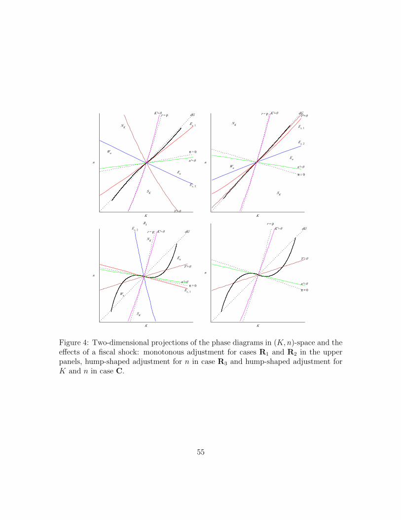
Figure 4: Two-dimensional projections of the phase diagrams in (K,n)-space and theeffects of a fiscal shock: monotonous adjustment for cases R1 and R2 in the upperpanels, hump-shaped adjustment for n in case R3 and hump-shaped adjustment forK and n in case C.

55

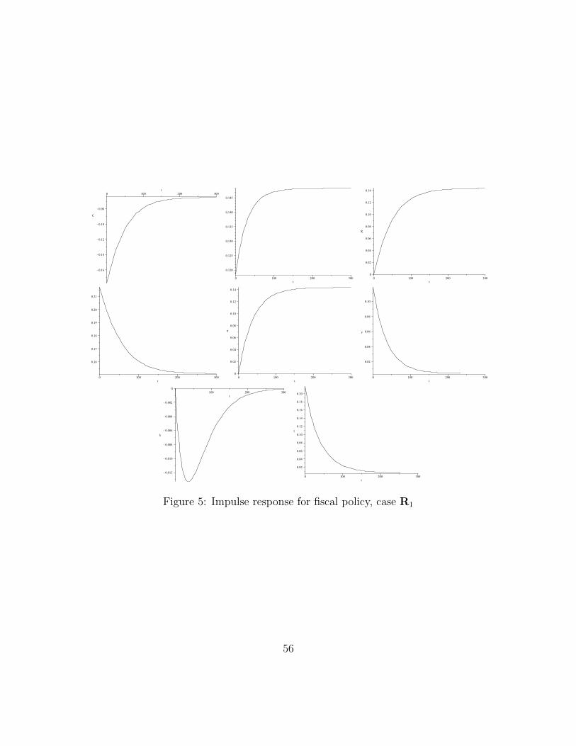
Figure 5: Impulse response for fiscal policy, case R1

56

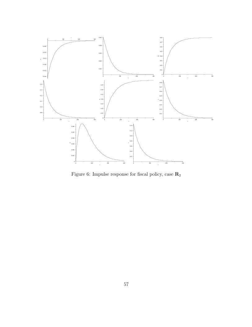
Figure 6: Impulse response for fiscal policy, case R2

57

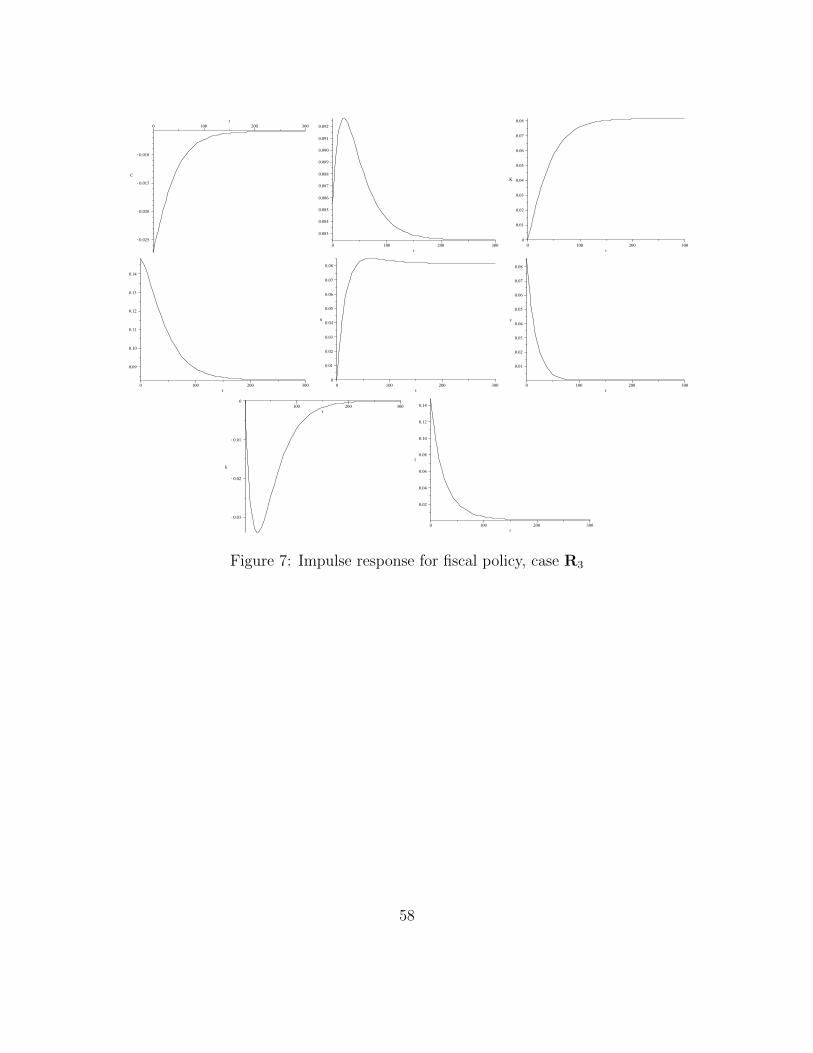
Figure 7: Impulse response for fiscal policy, case R3

58

Figure 8: Impulse response for fiscal policy, case C

59