Fiscal Policy and Economic Growth in Ethiopia

International Journal of African and Asian Studies www.iiste.org ISSN 2409-6938 An International Peer-reviewed Journal Vol.38, 2017

43

Fiscal Policy and Economic Growth in Ethiopia Getachew Petros Osebo Lecturer , Department of the economics, wolaita sodo university P. O Box 138 , wolaita sodo, Ethiopia ABSTRACT The purpose of the paper is to examine the impact of fiscal policy variables on economic growth for Ethiopia over the period 1974/75 – 2013/14, a period spanning 40 years. The fiscal policy variables considered components of government expenditure, revenue, and budget balance. To serve the objectives of the study Johnson’s Co integration test, VAR and VECM approaches are employed. The study result indicates that, economic growth and fiscal policy variables have long run relationship. Moreover the capital expenditure, direct tax and budget balance have positive relationship with economic growth in the long run. The main finding other tax has significance and positive impact on the country’s economic growth, In the short run, the error correction term come up with the expected sign and 43% of disturbances corrected each year. Based on the findings the study highlights some policy issues that policy makers should due attention. Key words : fiscal plicy ,economic growth , VAR model 1. INTRODUCTION 1.1 Background of the Study Ethiopia has currently become among one of the world’s fastest growing economies for numerous years, being driven by public sector investments and government supported growth initiatives. This has led to a remarkable improvement in the living standards of many peoples in the country, and the country’s infrastructure and overall domestic production is improving. Although, as indicated by KPMG (2014), the government’s growth strategy has received some criticism for crowding out private investment, and consequently hampering development of the private sector, the country’s overall growth prospects are still positive. Fiscal policy is one of those different variables that determine economic growth. According to Cristina and Michaela (2009), fiscal policy is defined as the deliberate manipulation of government income and expenditure to achieve economic and social objectives and sustain the country’s growth. In line with the above definition, Ethiopia’s growth strategy has focused towards economic and social development. Hence, pro-poor economic growth over the last decade has led to a considerable increase in per capita GDP and decrease in the national poverty rate. Significant progress has been made in achieving the MDGs, including: increased immunization and reduced child mortality; higher enrollment rates in primary schools; and better water sources and sanitation facilities (IMF, 2014). In recent years, the fiscal policy measures of the government has mainly focused on strengthening of domestic revenue mobilization and increasing on pro–poor spending. During 2010/11, the overall revenue mobilized by the government was Birr 85.6 billion, which was 99% of that indicated in the budget. The domestic revenue and grant components performed 104.5% and 82.5% of their corresponding annual plan, respectively. Particularly, tax revenue exhibited a good performance becoming 11.5% of the GDP compared to what it was in 2009/10 (11.3%); after showing a declining trend for the previous five years. Looking at the spending side, in 2010/11, a total of 40.5 billion Birr recurrent spending has been effected at the general government level, which constitutes 94% of the budget. During this period capital spending amounted to Birr 53.3 billion, making up 97% of the annual budget and showing an increase of Birr 32.3 billion (33%) compared with the performance in 2009/10. Capital spending has also constituted for about 57% of the total government budget in 2010/11. The overwhelming share of the expenditure (66%) was made to finance pro-poor spending. This resulted in a fiscal deficit of Birr 8.2 billion: a deficit that was well below the plan. The deficit was financed by 7.9 billion Birr (that is 1.5% of GDP) from external sources, while domestic financing was only 111millionBirr (that is 0.02% of GDP).Similarly, the total labor force of the country has increased by an average of about 2.2% per year between 1994/95 and 2007/08, which is slightly lower than the population growth rate. The urban labor force, taking the upper hand, increased at a higher rate (4.9%) than the rural labor force (1.9%). Thus, the share of urban labor force in total labor force increased from 10.4% in 1994/95 to 14.6% in 2007/08. Employed population increased from 25.8 million in1994/95 to 34 million in 2007/08 showing an average annual growth rate of 2.2%. This means, the rate of increase in the urban employment (5.4%) was higher than that of rural employment (1.8%); and the share of urban employment to total employment in the country has increased suggesting that more employment opportunities have been created in urban areas (MoFED, 2010). For the above achievements of the country, fiscal policy plays an important role as government uses fiscal policy as a method to influence and monitor the country’s economy by adjusting taxes and/or public spending. In doing so, the government can aim to find a balance between lowering unemployment and reducing the inflation rate. It is used by a government in an attempt to influence the direction of the economy through changes


44

in government taxes, or through some spending (fiscal allowances). Hence it can impact on the following variables in the economy: aggregate demand and the level of economic activity, the pattern of resource allocation and the distribution of income, also it has an impact on overall effect of the budget outcome on economic activity of the country (Badreldin, 2011). Furthermore, fiscal policy can play an important role in fostering economic growth in a view that government’s support for knowledge accumulation, research & development, productive investment, the maintenance of law and order and the provision of other public goods and services can stimulate growth in both the short-run and the long run (Easterly and Ribera, 1993; Mauro, 1995; Falster and Henderson, 1999).On the other hand, as pointed out by Matthew Kofi Oran (2009), fiscal policy is thought to stifle economic growth by distorting the effect of tax and inefficient government spending in the view that governments are inherently bureaucratic and less efficient and as a result they tend to hinder rather than facilitate growth if they get involved in the productive sectors of the economy. Hence, it is logical to empirically investigate the role or effect of fiscal policy on Ethiopia’s economic growth. 1.2 Objectives of the Study 1.2.1 General Objective of the Study The general objective of this study is to empirically investigate the effects of Ethiopia’s fiscal policies on the country’s economic growth for the period 1974/75-2013/14 fiscal years using, a period spanning 40 years. 1.2.2 Specific Objectives of the Study

Ø To identify whether fiscal policy variables has long run relationship with economic growth. Ø To examine the impact of fiscal policy on economic growth. Ø To examine the short run dynamics among fiscal policy variables on economic growth. Ø To forward feasible policy implications.

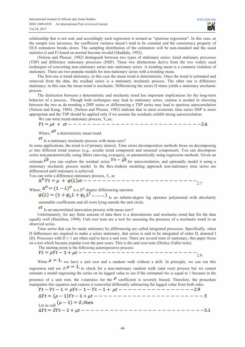
2. DATA AND METHODOLOGY This study aims at investigating the impact of fiscal policy instruments and economic growth relationship in Ethiopia and shall predict the cumulative effects taking into account the dynamic response among fiscal policy variables (tax revenue and expenditure components as well as budget deficit). To this end the study will use econometrics method known as the Johansen multivariate co integration model. The model specification, data sources and description, and estimation technique to be followed are described below. 2.1 Data sources and descriptions To carry out the estimation, annual time series data on labor force, gross capital formation, government revenue, and expenditure categories covering the period between 1974/75 and 2013/14 will be used. The secondary data included in this study were obtained from NBE (2013/14), and World Bank (WDI) data base (2013). 2.2 Data Analysis 2.3 Model Specification The estimated real GDP equation is specified based on endogenous growth models. That is, a model in which taxation and government spending can have effect on the rate of growth of per capita income, a proxy for economic growth. If output (Y) in the economy depends on the inputs of labor (L) and capital (K) and fiscal policy instrument (Z), then the production function for aggregate output can be presented as: ),,( tttt ZKLfY = -------------------------------------------------- (2.1) Kneller et al (1999:174) stated that “…in the empirical literature a specification issue has been frequently overlooked.” That is, previous researches used only one-side instruments of fiscal policy. Thus, they suggested that all fiscal policy variables have to be included in the regression. The importance is that the explicit and implicit financing of a unit change in an element of the government budget will affect the estimated coefficient. To put the point formally, growth, Ygit in country i at time t is a function of conditioning (non–fiscal) variables, L and K and a vector of fiscal variables, Zjt.

it

m

jjtjititogit uZKLY ++++= å

=121 bgga --------------------------- (2.2) When all elements of the budget (including the deficit/surplus) are included, then 01 =å=

m

jjtZ One element of Z in the estimation of equation (2.1 ) must be omitted in order to avoid perfect collinearity. In order to avoid perfect collinearity one element of Z in the estimation of equation (2.2) must be omitted. The


45

omitted variable is effectively the assumed compensating elements within the government’s budget constraint. Thus, we write equation (2.2) as å-

=

+++++=11210 m

jitmtmjtjititgit UZZKLY bbgga ----------------- (2.3) When we omit Zmtto avoid multicollinearity; then the identity 01 =å

=

m

jjtZ implies that the equation being actually estimated is

itjtmjititgit UZKLY ++++= å )_(210 bbgga --------------- (2.4) The standard hypothesis test of a zero coefficient of jtZ is in fact testing the null hypothesis that 0)( =- mj bb rather that 0=jb .The implication that it is possible to test only the different between the b values, and not each b individually does not exclude the possibility of testing weather two b values are equal. This is appropriate when theory suggests that there is more than one neutral category, in which case both b values are expects to be zero. If the hypothesis of equality cannot be rejected, then more precise parameter estimate can be obtained by omitting both categories. In this case, the correct interpretation of the coefficient on each fiscal category is that the effect of a unit change in the relevant variable offset by a unit change in the omitted category, which is the implicit financing element. However, if this is not done, and (for example) all expenditure variables are omitted from the regression and only tax variables are included (as in Mendoza et al, 1997) then the result will be biased because of the implicit partial financing by non-neutral elements of the government budget. On the other hand, if only some expenditure elements (such as capital expenditures) and budget deficit/surplus are omitted from the regression, then the result assumes implicitly that all included expenditures (i.e. recurrent/consumption expenditures) are equally unproductive; and all omitted capital expenditure and the budget surplus/deficit are “neutral” with respect to growth. In general, the appropriate procedure is to test down from the most complete specification of the government budget constraint to less complete specifications by ensuring to omit only those elements which theory suggests will have negligible (neutral) growth effect. Given the above justification for the inclusion of fiscal policy variables in the growth model, the complete real GDP equation is specified as ( )????? /ln,/ln,/ln,/ln,/ln,/ln,ln,lnln YBDYREYCEYOTYITYDTKLfRY

-++= . .. (2.5) Where: RGDP = growth domestic product L=Labor force actually engaged in production K=the ratio of private investment to nominal GDP

YDT / =The ratio of direct tax to nominal GDP YIT / =The ratio of indirect tax to nominal GDP YOT / =The ratio of other revenue (it includes foreign tax revenue, non-tax revenue and grants) to nominal GDP. YCE / = The ratio of public capital expenditure to nominal GDP YRE / =The ratio of public recurrent expenditure to nominal GDP YBE / =The ratio of primary budget deficit to nominal GDP All the variables are in logarithm form where there were some negative values in the all the years (eg budget deficits, the series were transformed in to positive value by adding scalar across the observations if were need to take logs. The variables and symbols are as defined above and the equation is linear in parameter. The expected signs of each variable is shown below the variable and “?” indicates an ambiguous sign. Economic growth is represented by real per capita income GDP.

2.2.2. Estimation Technique: 2.2.2.1 Unit Root Tests The classical time series regression model is based on the assumption that the data generating processes are stationary, i.e., the moments of the variables under consideration are time invariant. However, as the economy grows and evolves over time, most macroeconomic variables are likely to grow over time rendering them non-stationary (Granger and New bold, 1974). Regression using non-stationary variables will only reflect a


46

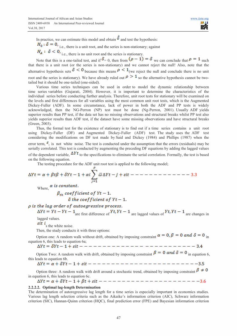
relationship that is not real, and accordingly such regression is termed as “spurious regression”. In this case, as the sample size increases, the coefficient variance doesn’t tend to be constant and the consistency property of OLS estimators breaks down. The sampling distribution of the estimators will be non-standard and the usual statistics (t and F) based on normal become invalid (Maddala, 1992). (Nelson and Plosser, 1982) distinguish between two types of stationary series: trend stationary processes (TSP) and difference stationary processes (DSP). These two distinctions derive from the two widely used techniques of converting non-stationary series into stationary series. A trending mean is a common violation of stationary. There are two popular models for non-stationary series with a trending mean. The first one is trend stationary; in this case the mean trend is deterministic. Once the trend is estimated and removed from the data, the residual series is a stationary stochastic process. The other one is difference stationary; in this case the mean trend is stochastic. Differencing the series D times yields a stationary stochastic process. The distinction between a deterministic and stochastic trend has important implications for the long-term behavior of a process.. Though both techniques may lead to stationary series, caution is needed in choosing between the two as de-trending a DSP series or differencing a TSP series may lead to spurious autocorrelation (Nelson and Kang, 1984). (Nelson and Plosser, 1982) indicate that in most economic time series DSP is more appropriate and the TSP should be applied only if we assume the residuals exhibit strong autocorrelation.We can write trend-stationary process, Yt,as; Where, a deterministic mean trend. Is a stationary stochastic process with mean zero? In some applications, the trend is of primary interest. Time series decomposition methods focus on decomposing μt into different trend sources (e.g., secular trend component and seasonal component). You can decompose series non-parametrically using filters (moving averages), or parametrically using regression methods. Given an estimate pa you can explore the residual series ag ), for autocorrelation, and optionally model it using a stationary stochastic process model. In the Box-Jenkins modeling approach non-stationary time series are differenced until stationary is achieved. You can write a difference-stationary process, Yt, as ry pr s, 2.7 Where, is a Dth-degree differencing operator. gr Is an infinite-degree lag operator polynomial with absolutely summable coefficients and all roots lying outside the unit circle. Is an uncorrelated innovation process with mean zero? Unfortunately, for any finite amount of data there is a deterministic and stochastic trend that fits the data equally well (Hamilton, 1994). Unit root tests are a tool for assessing the presence of a stochastic trend in an observed series. Time series that can be made stationary by differencing are called integrated processes. Specifically, when D differences are required to make a series stationary, that series is said to be integrated of order D, denoted I (D). Processes with D ≥ 1 are often said to have a unit root. There are several tests of stationary, this paper focus on a test which became popular over the past years: This is the unit root tests (Dickey-Fuller tests). The starting point is the following autoregressive process: ng po g gr pr 2.8. When we have a unit root and a random walk without a drift. In principle, we can run this regression and see ifif to check for a non-stationary random walk (unit root) process but we cannot estimate a model regressing the series on its lagged value to see if the estimated rho is equal to 1 because in the presence of a unit root, the t-statistics for the coefficient is severely biased. Therefore, the procedure manipulate this equation and express it somewhat differently subtracting the lagged value from both sides. Let us call


47

In practice, we can estimate this model and obtain and test the hypothesis: pr , i.e., there is a unit root, and the series is non-stationary; against i.e., there is no unit root and the series is stationary. Note that this is a one-tailed test, and if = 0, then from ry we can conclude that such that there is a unit root (or the series is non-stationary) and we cannot reject the null! Also, note that the alternative hypothesis sets because this means ry) (we reject the null and conclude there is no unit root and the series is stationary). We have already ruled out so the alternative hypothesis cannot be two-tailed but it should be one-tailed (one-sided). Various time series techniques can be used in order to model the dynamic relationship between time series variables (Gujarati, 2004). However, it is important to determine the characteristics of the individual series before conducting further analysis. Therefore, unit root tests for stationary will be examined on the levels and first differences for all variables using the most common unit root tests, which is the Augmented Dickey-Fuller (ADF). In some circumstance, lack of power in both the ADF and PP tests is widely acknowledged, then the NG-Perron (NP) test must be done (Ng-Perron, 2001). Usually ADF yields superior results than PP test, if the data set has no missing observations and structural breaks whilst PP test also yields superior results than ADF test, if the dataset have some missing observations and have structural breaks (Green, 2003). Thus, the formal test for the existence of stationary is to find out if a time series contains a unit root using Dickey-Fuller (DF) and Augmented Dickey-Fuller (ADF) test. The study uses the ADF test considering the modifications on DF test made by Said and Dickey (1984) and Phillips (1987) when the error term, g t is not white noise. The test is conducted under the assumption that the errors (residuals) may be serially correlated. This test is conducted by augmenting the preceding DF equations by adding the lagged values of the dependent variable, to the specifications to eliminate the serial correlation. Formally, the test is based on the following equation. The testing procedure for the ADF unit root test is applied to the following model; Where, are first difference of are lagged values of are changes in lagged values. gg s the white noise. Then, the study conducts it with three options: Option one: A random walk without drift, obtained by imposing constraint in equation 6, this leads to equation 6a; Option Two: A random walk with drift, obtained by imposing constraint in equation 6, this leads to equation 6b. Option three: A random walk with drift around a stochastic trend, obtained by imposing constraint in equation 6, this leads to equation 6c. 2.2.2.2. Optimal lag-length Determination The determination of autoregressive lag length for a time series is especially important in economics studies. Various lag length selection criteria such as the Aikaike’s information criterion (AIC), Schwarz information criterion (SIC), Hannan-Quinn criterion (HQC), final prediction error (FPE) and Bayesian information criterion


48

(BIC) have been employed. As the outcomes of these criteria may influence the ultimate findings of a study, a throughout understanding on the empirical performance of these criteria is warranted. As a result, another key element in a model specification process is to determine the correct lag length. Several studies in this area demonstrate the importance of selecting a correct lag length. Estimates of the model would be inefficient and inconsistence if the selected lag length is different from the true lag length (Brooks, 2004). Selecting a higher order lag length than the true one over estimates the parameter values and increases the forecasting errors and selecting a lower lag length usually underestimate the coefficients and generates auto-correlated errors. Therefore, accuracy of parameters and forecasts heavily depend on selecting the true lag length. Though, there are so many criteria usedin the literature to determine the lag length of an AR process. Criteria’s the study uses are as follows. Criteria one: Akaike’s Information Criterion Criteria two: Schwarz Information criterion Criteria three: Hannan-Quinn criterion Criteria four: Final prediction error Where, is the sample size, Is the model’s residual. Akaike Information Criterion (AIC) developed by Hirotugu Akaike in 1971 (Greene, 2003) ,has been found to be nearly unbiased estimator of selecting lag order and also it’s a large sample size measure of thirty and more items, while the Schwarz Information Criterion (SIC) is a small sample measure of less than thirty observations. (Liew& Venus Khim−Sen, 2004), provide useful insights for empirical researchers. First, these criteria managed to pick up the correct lag length at least half of the time in small sample. Second, this performance increases substantially as sample size grows. Third, with relatively large sample (120 or more observations), HQC is found to outdo the rest in correctly identifying the true lag length. In contrast, AIC and FPE should be a better choice for smaller sample. Fourth, AIC and FPE are found to produce the least probability of under estimation among all criteria under study. Finally, the problem of over estimation, however, is negligible in all cases. As many econometric testing procedures such as unit root tests, causality tests, Cointegration tests and linearity tests involved the determination of autoregressive lag lengths, the findings in this simulation study may be taken as useful guidelines for future economic researches. Hence, the ability to correctly locating the true lag length depends on IC the ordinary least Squares regression model has been run starting with lag zero upwards, since according to (Engle et al, 1995) it is the mostly used and recommended methodology used to determine the lag length. Accordingly, lag that provides the minimum value is chosen as the optimal lag length, in other words, among the IC that provides majority lag has been chosen as optimal lag length. 2.2.2.2 Cointegration tests: Johansen’s procedure On the basis of the theory that integrated variables of order one, I(1), may have a Cointegration relationship, it is crucial to test for the existence of such a relationship. If a group of variables are individually integrated of the same order and there is at least one linear combination of these variables that is stationary, then the variables are said to be co integrated. The co integrated variables will never move far apart, and will be attracted to their long-run relationship. Testing for Cointegration implies testing for the existence of such a long-run relationship between economic variables. This study considers a number of Co integration tests, namely the Engle-Granger method commonly known as the two-step estimation procedure, the Phillips-Ouliaris methods and the Johansen's procedure. This study used Johansen’s procedure in order to determine long run relationship between series. Since the influential work of (Granger &New bold, 1974) and (Engle and Granger, 1987) on the treatment of integrated time series data, many studies have been conducted using the co-integration methodology in order to yield consistent results and avoid the spurious regression problems, particularly in causality testing. The purpose of co-integration test in this study is to examine whether economic growth and tax revenue share a common stochastic trend, that is, whether they move on the same wave-length in the long-run though there might be some disequilibrium in the short-run. This research will employ (Johansen’s, 1988) approach to determine whether any combinations of the variables are co-integrated.


49

(Johansen & Juselius, 1990) recommend the trace test and the maximum Eigen-value t-statistics in making the inference of the number of co-integrating vectors. Johansen’s methodology takes its starting point in the Vector Autoregression (VAR) of order given by: Where Yt is an vector of variables that are integrated of order one-commonly denoted I(1) and is an vector of innovations. Reparameterising equation 6, that is, subtracting Yt-1 on both sides leads to Where, and, If the coefficient matrix Π has reduced rank r < n, then there exist n x r matrices α and β each with rank r such that Π = ’ and is stationary. Is the number of cointegrating relationships, the elements of are known as the adjustment parameters in the vector error correction model and each column of is a cointegrating vector. It can be shown that for a given r, the maximum likelihood estimator of defines the combination of that yields the r largest canonical correlations of with after correcting for lagged differences and deterministic variables when present. Johansen proposes two different likelihood ratio tests of the significance of these canonical correlations and thereby the reduced rank of the Π matrix: the trace test and maximum eigenvalue test, shown in equations (5) and (6) respectively. Here is the sample size and is the largest canonical correlation. The trace test tests the null hypothesis of cointegrating vectors against the alternative hypothesis of cointegrating vectors. The maximum eigenvalue test, on the other hand, tests the null hypothesis of co integrating vectors against the alternative hypothesis of 1 + cointegrating vectors. For trace statistic, the null hypothesis is the number of co-integrating vectors is less than or equal to co-integrating vectors (r) against an unspecified alternative. In the case of maximum Eigen-value co-integration test, the null hypothesis is the number of co-integrating vectors (r) against the alternative of 1 + r (Ng et al, 2008). If the trace statistic is greater that the Eigen-value (critical value), we conclude that the model contains at least one co-integrating equation. Where this condition is violated at a higher order, determines the maximum number of co-integrating equations. Therefore, procedures in accordance with Johansen approach will be used in this study. Finally, since the long run equilibrium may rarely be observed the short run dynamic/evolution of the variables under consideration is considered. For this reason, an ECM is extended to the multivariate scenario by defining all the variables to be potentially endogenous. In order to arrive at the short run final preferred model, a one period lag of the Cointegration vector saved from the long run estimation enters in ECM estimation using OLS. Therefore, we can use the t-distribution of the parameter estimate of the VECM as the conventional properties of the distribution hold asymptotically.

2.2.2.4 Short-Run Co-Integration: Vector Error Correction Model (VECM) The dynamic relationship includes the lagged value of the residual from the co integrating regression ( 1-tECT ) in addition to the first difference of variables which appear in the right hand side of the long-run relationship in model (3.5). The inclusion of the variables from the long-run relationship would capture short-run dynamics. In order to arrive at the short-run final preferred model, a one period lag of the co integration vector saved from the


50

long run estimation will enter in ECM estimation using OLS. The dynamic specification of the model allows the deletion of the insignificant variables, while the error correction term is retained. The final form of the vector error-correction model (VECM) will be selected according to the general to specific methodology suggested by Harris (1995).The size of the error correction term indicates the speed of adjustment of any disequilibrium towards a long-run equilibrium state (Engle and Granger, 1987). The general form of the vector error correction model (VECM) for the growth model is specified as follows: åå ååå== ==

-

=

+D+D+D++D+D+=Dk

i

k

i

k

it

dt

k

iit

k

iYOTYITYDTkLy 1 51 1 431 21 10 /ln/ln/lnlnln bbbbba

tt

k

i

k

i

k

iECTYBDYREYCE ebbb ++D+D+D -

===

ååå 11 81 71 6 /ln/ln/ln --------- (7 ) Where D is the first difference operator, 1-tECT is the error correction term lagged one period,g is the short-run coefficient of the error correction term )01( <<- g , te and tv are the white noise terms of respective models. At the end of each short-run models the stability of the parameters will be examined using recursive technique.

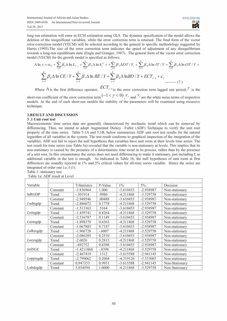
3.RESULT AND DISCUSSION 3 .1 Unit root test Macroeconomic time series data are generally characterized by stochastic trend which can be removed by differencing. Thus, we intend to adopt Augmented Dickey –Fuller (ADF) Technique to verify the unit root property of the time series. Table 5.1A and 5.1B, below summarizes ADF unit root test results for the natural logarithm of all variables in the system. The test result conforms to graphical inspection of the integration of the variables. ADF test fail to reject the null hypothesis that variables have unit roots at their levels time series. The test result for time series (see Table 3a) revealed that the variable is non-stationary at levels. This implies that its non-stationary is caused by the presence of a deterministic time trend in its process, rather than by the presence of a unit root. In this circumstance the series does not need differencing to make it stationary, just including as additional variable in the test is enough. As indicated in Table 1b, the null hypotheses of unit roots at first differences are soundly rejected at 1% and 5% critical values for all-time series variable. Hence the series are integrated of order one i.e. I (1). Table 1: stationary test Table 1a: ADF result at Level Variable T-Statistics P-Value 1% 5% Decision lnRGDP Constant -3.836964 1.000 -3.610453 -2.938987 Non-stationary Trend -.301914 .9980 -4.211868 -3.529758 Non-stationary Lndtsgdp Constant -2.949546 .00488 -3.610453 -2.938987 Non-stationary Trend -2.886072 0.1778 -4.211868 -3.529758 Non-stationary Lnitsgdp Constant -1.513363 .5164 -3.610453 -2.938987 Non-stationary Trend -1.459741 0.8264 -4.211868 -3.529758 Non-stationary Lnotsgdp Constant -2.536787 0.1149 -3.610453 -2.938987 Non-stationary Trend -1.898379 0.6363 -4.211868 -3.529758 Non-stationary LnResgdp Constant -1.067885 0.7187 -3.610453 -2.938987 Non-stationary Trend -1.966728 -.6007 -4.211868 -3.529758 Non-stationary Lncesgdp Constant -2.086285 0.2510 -3.610453 -2.938987 Non-stationary Trend -2.6026 0.2813 -4.211868 -3.529758 Non-stationary lnSSGE Constant -.692752 0.8398 -3.610453 -2.938987 Non-stationary Trend -1.4211868 -.8398 -4.211868 -3.529758 Non-stationary Lnppisgdp Constant -2.467419 .1312 -3.615588 -2.941145 Non-stationary Trend -2.799062 0.2064 -4.219126 -3.533083 Non-stationary Lnbdsgdp Constant 0.947353 0.9951 -3.615588 -2.941145 Non-Stationary Trend 5.034594 1.0000 -4.211868 -3.529758 Non-Stationary


51

Table 1b: ADF result at first difference Variable T-Statistics P-Value 1% 5% Decision ∆lnRGDP Constant -4.278287* 0.0017** -3.615588 -2.941145 I(1) Trend -6.285638* 0.0000** -4.226815 -3.536601 I(1) ∆lndtsgdp Constant -8.124615* 0.00000** -3.615588 -2.941145 I(1) Trend -8.079984* 0.0000** -4.219126 -3.533083 I(1) ∆lnitsgdp Constant -5.386521* 0.00001** -3.615588 -2.941145 I(1) Trend -5.302275* 0.0006** -4.219126 -3.533083 I(1) ∆lnotsgdp Constant -5.309939* 0.0001** -3.615588 -2.941145 I(1) Trend -5.584056* 0.0003** -4.219126 -3.533083 I(1) ∆lnResgdp Constant -5.400513* 0.0001** -3.615588 -2.941145 I(1) Trend -5.624126* 0.0002** -4.219126 -3.533083 I(1) ∆lncesgdp Constant -5.706773* 0.0000** -3.615588 -2.941145 I(1) Trend -5.673157* 0.0002** -4.219126 -3.533083 I(1) ∆lnSSGE Constant -6.559788* 0.0000** -3.615588 -2.941145 I(1) Trend -6.616673* 0.0000** -4.219126 -3.533083 I(1) ∆lnppisgdp Constant -12.53498* 0.0000** -3.615588 -2.941145 I(1) Trend -12.53918* 0.0000** -4.219126 -3.533083 I(1) ∆lnbdsgdp Constant -10.38628* .0000** -3.615588 -2.941145 I(1) Trend -10.58645* 0.000** -4.219126 -3.198312 I(1)

Source: own computation using EVIews version 6 Note: * indicates level of significance (rejection of the null hypothesis) at 1 and 5%, while ** indicates level of significance (rejection of the null hypothesis) at both 1 & 5%. Therefore, from the above table one can conclude that all the variables are non-stationary at level. That is, the test conducted fails to reject the null hypothesis of unit root both constant and with trend. However, the ADF test shows that their first difference is stationary at conventional 1% and 5% level of significance. So the variables are, integrated of order one I (1).Then, since all the variables are I(1), Johansen multivariate co-integration test can be used to find out whether there exist a long-run relationship between the variables or not. The linear combination of I(1) variables will be stationary if variables are co-integrated (Harris, 1995).

3.2. Lag Length Selection Table below summarizes results of standard lag length selection criteria in unrestricted VAR model adopting a general to specific procedure. While SBIC criteria select one lags, the remaining four criteria suggest two lags. Despite the fact that SBIC will deliver the correct model with few lags as compared to AIC we must make sure that lags with significance information. Table 2: Lag length selection VAR Lag Order Selection Criteria Endogenous variables: LNRGDP LNRESGDP LNCESGDP LNDTSGDP LNITSGDP LNOTSGDP LNPISGDP LNSSGE LNBDSGDP Exogenous variables: C Sample: 40 Included observations: 38 Lag LogL LR FPE AIC SC HQ 0 -22.61632 NA 4.27e-11 1.664017 2.051866 1.802011 1 216.1840 351.9163 1.18e-14 -6.641263 -2.762770* -5.261325 2 333.4520 117.2680* 3.80e-15* -8.550105* -1.180967 -5.928222* Note: * indicates lag order selected by the criterion FPE: Final prediction error


52

4.3. Long run Relationship-Johansen Co integration test Johansen co integration test result in order to avoid spurious estimates, we intend to established long run relation among the variable. Having detected the non-stationary behavior of all the series and chosen the optimal lag length, the test of co-integration was conducted for the variables under investigation. Table 3a shows the results obtained from applying the Johansen co integration tests for all the variables under study. To determine the number of co integration vectors two test statistics called the maximum eigenvalue (λmax) and trace statistics (trace) are computed. Table 3: Johansen co integration Series: LNRGDP LNRESGDP LNCESGDP LNBDSGDP LNDTSGDP LNITSGDP LNOTSGDP LNPISGDPLNSSGE Lags interval (in first differences): 1 to 1 Unrestricted Co integration Rank Test (Maximum Eigen value) Hypothesized Max-Eigen 0.05 No. of CE(s) Eigenvalue Statistic Critical Value Prob.** None * 0.938737 106.1177 58.43354 0.0000 At most 1 * 0.855410 73.48645 52.36261 0.0001 At most 2 0.664899 41.54633 46.23142 0.1460 At most 3 0.622070 36.97571 40.07757 0.1073 At most 4 * 0.590748 33.95016 33.87687 0.0490 At most 5 0.370560 17.59116 27.58434 0.5295 At most 6 0.227651 9.816136 21.13162 0.7617 At most 7 0.147220 6.051642 14.26460 0.6066 At most 8 5.24E-05 0.001990 3.841466 0.9610 Max-eigenvalue test indicates 2 co integrating eqn(s) at the 0.05 level * denotes rejection of the hypothesis at the 0.05 level **MacKinnon-Haug-Michelis (1999) p-values From the Johansen maximum Eigen statistics perspective, the result suggests that the null hypothesis of one co integration vector can be rejected at the 5 per cent significant level. The maximum Eigen value test makes the confirmation of this result that led to the conclusion of two ranks, i.e. two co integration relationships for model under investigation implying the variables included in the model have long-run or equilibrium relationship among the variables. This result therefore is in agreement with similar study in Nigeria conducted by amin u and anono (2012). The above Table 3a, shows that, in the long run economic growth has a positive relationship with capital expenditure, private investment, primary budget balance, direct tax, school enrollment and has a negative relationship with , indirect tax , other tax , recurrent expenditure .The results suggest by elasticity concepts that’s one percent increase in capital expenditure , direct tax ,private investment, primary budget deficit and school enrollment leads to increase in the real GDP by80% ,16%,44%,63%and 17% respectively.


53

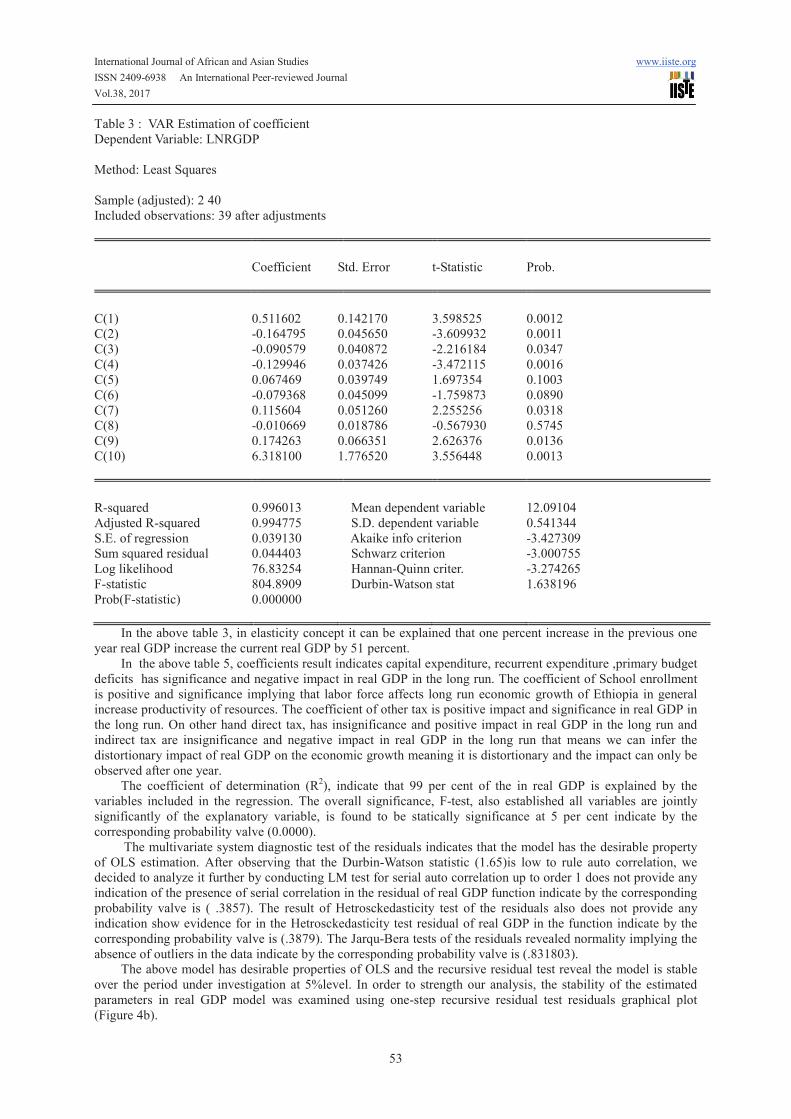
Table 3 : VAR Estimation of coefficient Dependent Variable: LNRGDP Method: Least Squares Sample (adjusted): 2 40 Included observations: 39 after adjustments Coefficient Std. Error t-Statistic Prob. C(1) 0.511602 0.142170 3.598525 0.0012 C(2) -0.164795 0.045650 -3.609932 0.0011 C(3) -0.090579 0.040872 -2.216184 0.0347 C(4) -0.129946 0.037426 -3.472115 0.0016 C(5) 0.067469 0.039749 1.697354 0.1003 C(6) -0.079368 0.045099 -1.759873 0.0890 C(7) 0.115604 0.051260 2.255256 0.0318 C(8) -0.010669 0.018786 -0.567930 0.5745 C(9) 0.174263 0.066351 2.626376 0.0136 C(10) 6.318100 1.776520 3.556448 0.0013 R-squared 0.996013 Mean dependent variable 12.09104 Adjusted R-squared 0.994775 S.D. dependent variable 0.541344 S.E. of regression 0.039130 Akaike info criterion -3.427309 Sum squared residual 0.044403 Schwarz criterion -3.000755 Log likelihood 76.83254 Hannan-Quinn criter. -3.274265 F-statistic 804.8909 Durbin-Watson stat 1.638196 Prob(F-statistic) 0.000000 In the above table 3, in elasticity concept it can be explained that one percent increase in the previous one year real GDP increase the current real GDP by 51 percent. In the above table 5, coefficients result indicates capital expenditure, recurrent expenditure ,primary budget deficits has significance and negative impact in real GDP in the long run. The coefficient of School enrollment is positive and significance implying that labor force affects long run economic growth of Ethiopia in general increase productivity of resources. The coefficient of other tax is positive impact and significance in real GDP in the long run. On other hand direct tax, has insignificance and positive impact in real GDP in the long run and indirect tax are insignificance and negative impact in real GDP in the long run that means we can infer the distortionary impact of real GDP on the economic growth meaning it is distortionary and the impact can only be observed after one year. The coefficient of determination (R2), indicate that 99 per cent of the in real GDP is explained by the variables included in the regression. The overall significance, F-test, also established all variables are jointly significantly of the explanatory variable, is found to be statically significance at 5 per cent indicate by the corresponding probability valve (0.0000). The multivariate system diagnostic test of the residuals indicates that the model has the desirable property of OLS estimation. After observing that the Durbin-Watson statistic (1.65)is low to rule auto correlation, we decided to analyze it further by conducting LM test for serial auto correlation up to order 1 does not provide any indication of the presence of serial correlation in the residual of real GDP function indicate by the corresponding probability valve is ( .3857). The result of Hetrosckedasticity test of the residuals also does not provide any indication show evidence for in the Hetrosckedasticity test residual of real GDP in the function indicate by the corresponding probability valve is (.3879). The Jarqu-Bera tests of the residuals revealed normality implying the absence of outliers in the data indicate by the corresponding probability valve is (.831803). The above model has desirable properties of OLS and the recursive residual test reveal the model is stable over the period under investigation at 5%level. In order to strength our analysis, the stability of the estimated parameters in real GDP model was examined using one-step recursive residual test residuals graphical plot (Figure 4b).


54

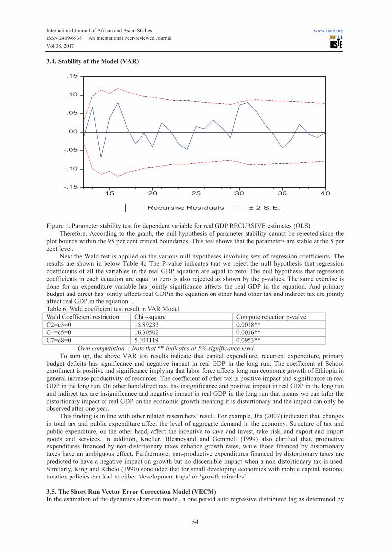
3.4. Stability of the Model (VAR)

-.15-.10-.05.00.05.10.15

15 20 25 30 35 40Recursive Residuals ± 2 S.E. Figure 1. Parameter stability test for dependent variable for real GDP RECURSIVE estimates (OLS) Therefore, According to the graph, the null hypothesis of parameter stability cannot be rejected since the plot bounds within the 95 per cent critical boundaries. This test shows that the parameters are stable at the 5 per cent level. Next the Wald test is applied on the various null hypotheses involving sets of regression coefficients. The results are shown in below Table 4c The P-value indicates that we reject the null hypothesis that regression coefficients of all the variables in the real GDP equation are equal to zero. The null hypothesis that regression coefficients in each equation are equal to zero is also rejected as shown by the p-values. The same exercise is done for an expenditure variable has jointly significance affects the real GDP in the equation. And primary budget and direct has jointly affects real GDPin the equation on other hand other tax and indirect tax are jointly affect real GDP.in the equation. . Table 6: Wald coefficient test result in VAR Model Wald Coefficient restriction Chi –square Compute rejection p-valve C2=c3=0 15.89233 0.0018** C4=c5=0 16.30502 0.0016** C7=c8=0 5.104119 0.0953** Own computation : Note that ** indicates at 5% significance level. To sum up, the above VAR test results indicate that capital expenditure, recurrent expenditure, primary budget deficits has significance and negative impact in real GDP in the long run. The coefficient of School enrollment is positive and significance implying that labor force affects long run economic growth of Ethiopia in general increase productivity of resources. The coefficient of other tax is positive impact and significance in real GDP in the long run. On other hand direct tax, has insignificance and positive impact in real GDP in the long run and indirect tax are insignificance and negative impact in real GDP in the long run that means we can infer the distortionary impact of real GDP on the economic growth meaning it is distortionary and the impact can only be observed after one year. This finding is in line with other related researchers’ result. For example, Jha (2007) indicated that, changes in total tax and public expenditure affect the level of aggregate demand in the economy. Structure of tax and public expenditure, on the other hand, affect the incentive to save and invest, take risk, and export and import goods and services. In addition, Kneller, Bleaneyand and Gemmell (1999) also clarified that, productive expenditures financed by non-distortionary taxes enhance growth rates, while those financed by distortionary taxes have an ambiguous effect. Furthermore, non-productive expenditures financed by distortionary taxes are predicted to have a negative impact on growth but no discernible impact when a non-distortionary tax is used. Similarly, King and Rebelo (1990) concluded that for small developing economies with mobile capital, national taxation policies can lead to either ‘development traps’ or ‘growth miracles’. 3.5. The Short Run Vector Error Correction Model (VECM) In the estimation of the dynamics short-run model, a one period auto regressive distributed lag as determined by


55

the information criteria was initially imposed on all variables. The vector error term saved from the long run equation also entered in its first lag. Since all the variables are statistically significant in the long run Johansen co integration test no variable is conditioned in the short-run model. Then, the Hendry general to specific (Gets) procedure, which involves simplifying the model into a more interpretable characterization of the data by reducing sequentially insignificant variables based on t-value was used. At each stage of reduction F-test for model evaluation and diagnostic test are carried out to check that the reduction is reasonable. Table 3a above presents the results of the VECM for the real GDP in the function. The results reveal that all the variables included in the dynamic short-run model except the lag of change in real GDP are statistically in significant in affecting real GDP in the function. In the above table 5a show that the indirect tax, recurrent expenditure, capital expenditure has statistically insignificant and has negative impact on economic growth in the short-run , the direct tax ,other tax has statistically significant and has positive impact on economic growth in the short-run . The speed of adjustment has also a negative sign and its magnitude is not greater than unity. It implies that 43 per cent of the disturbance in the short run will be corrected each year. The coefficient of determination (R2), indicate that 66 per cent of the growth in real GDP is explained by the variables included in the regression. The overall significance, F-test, also established all variables are jointly significantly of the explanatory variable, is found to be statically significance at 5 per cent indicate by the corresponding probability valve (0.000604*). The multivariate system diagnostic test of the residuals indicates that the model has the desirable property of OLS estimation. For instance, the LM test for serial autocorrelation does not provide any indication of the presence of serial correlation in the residual of real GDP function. Indicate by the corresponding probability a valve (0.4511) how that does not provide any indication of the presence of serial correlation in the residual of real GDP in the function.).The result of Hetrosckedasticity test of the residuals also does not provide any indication show evidence for in the Hetrosckedasticity test residual of real GDP function. Indicate by the corresponding probability valve (0.522279) The Jarqu-Bera tests of the residuals revealed normality implying the absence of outliers in the data. Indicate by the corresponding probability valve (0.4008). 4. CONCLUSION AND POLICY IMPLICATION 4.1 Conclusion The main purpose of this study was to empirically examine the impact of fiscal policy variables on economic growth in Ethiopia over the period 1974/75-2013/14. In order to avoid spurious estimates, the unit roots of the series, were verified using Augmented Dickey –Fuller (ADF) technique after which Co integration was conducted. The study has employed the Johansen approach to test for the likelihood of long run relation among the variables. After the long run relation among the variable verified, both VAR and VECM approaches followed in order to capture the long run as well as short run dynamics of the variables. The long run (VAR) test result showed that, real GDP has positive relation with capital expenditure, direct tax, government budget balance, private investment and school enrollments while negatively related with other tax, indirect tax as well as recurrent expenditure with economic growth. The outcome indicates two findings: first other tax has significance and positive impact on the economic growth in the long run. Second school enrollment has significance and positive impact on economic growth in the long run .on other hand, in the short run: first, other tax has significant and positive impact on the economic growth. Second direct tax has significant and positive impact on the economic growth. 4.2 Recommendation Based on the above findings, the following are the recommendations of the study: Considering the current state of Ethiopia’s economy, capital expenditure should be greater than recurrent expenditure in order to lay the foundation for sustainable development and growth. There is need for rational utilization of the nation’s resources. Furthermore, expenditures on items/activities that are irrelevant or have no significant linkage to growth should be avoided. Higher budgetary allocation to capital formation is not just what is needed. Utilization of disbursed funds meant for capital projects should be closely monitored, especially in the area of procurement (of goods, services and works). Strong (effective and efficient) mechanism should be put on ground to ensure that the poor who are in the majority benefit from the expenditures of the federal government, as the state exists for the common good and none should be excluded from the benefits it offers. This is necessary to enhance improved welfare as the welfare of the people is a veritable ingredient for a robust economy. Transparency, rationality, responsiveness, equity, accountability, efficiency, adherence to the rule of law, economy, should be the guiding principles in the utilization of public funds. Until these are observed, the intended objectives and goals of government expenditure will not be realized.


56

References ABC of Taxes in Ethiopia (1942-1996). Addis Ababa: Planning & Research Department, Ministry of Finance. AfDB (2004). “African Economic Outlook, African Development Bank.” Pp 133- 146. Alan J.Auerbach (2005).“The Effectiveness of Fiscal Policy as Stabilization Policy.”University of California, Berkeley. Alemayehu.G & Abebe.S. (2005). Tax and Tax Reform in Ethiopia, 1990-2003. UN WIDER, Research paper No.2005/65. Alemayehu Geda and KibromTafere (2008). “The Galloping Inflation in Ethiopia: A Cautionary Tale for Aspiring ‘Developmental States’ in Africa.” Working Paper Series No. A01/2011, Institute of African Economic Studies (IAES) and Addis Ababa University (2008). Alesina, A. and S. Ardagna (1998). Tales of Fiscal Contractions. Economic Policy, vol.27, 487—545. Aminu, U. and A.Z. Anono (2012).An empirical Analysis of The Relationship between Unemployment and Inflation in Nigeria from 1977-2009. Business Journal, Economics and Review, Vol.1 (12), pp 42-61. Global Research Society. Pakistan. Ardagna, S. (2007). Fiscal policy in unionized labor markets. Journal of Economic Dynamics and Control 31, 1498/1534. Badreldin Mohamed Ahmed Abdurrahman, Fiscal Policy and Economic Growth in Sudan, 1996-2011 Barro, R. (1990) Government Spending in a Simple Model of Endogenous Growth. Journal of Political Economy Barro, R. J. (1989). The Ricardian Approach to Budget Deficits. The Journal of Economic Perspectives Barro, R.andSala-i-Martins, X. (1991).Convergence across States and Regions. Brooks Paper son Economic Activities,1, 107-182. Beetsma, 2009 Beetsma, R. (2008). “A survey of the effects of discretionary fiscal policy."Working Paper University of Amsterdam. Bailey J (2002). Public sector economics: theory, policy and Practice. Great Britain: Palgrave Macmillan. 2nd Ed. Ministry of Finance (1997). Blinder, A.S. and Solow, R.M., (2005), “Does fiscal policy matter? In A. Bagchi, ed., Readings in Public Finance. New Delhi:Oxford University Press, 283-300. Carvalho, M. et al. (2009). Non-Keynesian Effects of Fiscal Policy in a New Keynesian General Equilibrium Model for the Euro Area. Doctoral Thesis, Faculdade de Economia da Universidade do Port Demirew, Getachew (2004). Tax Reform in Ethiopia & Progress to Date. Addis Ababa: Ethiopian Economics Association. International Conference on Ethiopian Economy June 3-4. Devereux, Michael B., Head, Allan C. and Beverly J.Lapham (1996). Monopolistic Competition, Increasing Returns, and the Effects of Government Spending. Journal of Money, Credit, and Banking 28, 2, 233-254. Dickey D.A and Fuller W.A (1979). Distribution of the Estimators for Autoregressive Time series with a unit root. Journal of American Statistical Association, Volume 74. Easterly, W., and Rebelo, S. (1993) Fiscal Policy and Economic Growth. Journal of Monetary Economics Engle, RF & Granger, CWJ. (1987). Co-integration and error correction: representation, estimation and testing. Econometrica, vol. 55, no. 2, pp. 251-276. Fatás, A., and Mihov, I. (2001) The Effects of Fiscal Policy on Consumption and Employment: Theory and Evidence [online]. Available from: http://www.insead.edu/facultyresearch/faculty/personal/imihov/documents/FPandConsumptionAug2001.pdf Feldstein, M. (1982). Government Deficits and Aggregate Demand. Journal of Monetary Economics, vol. 9(1), 1—20. Galí, Jordi, Vallés, Javier, and J.D. López-Salido (2007). Understanding the Effects of Government Spending on Consumption. Journal of the European Economic Association 5, 1, 227-70. Gemmell, N., R. Kneller and I. Sanz (2006). Fiscal Policy Impacts on Growth in the OECD: Are They Long- or Short-Term?. Mimeo, University of Nottingham 2006. Geoffrey et al., (2006). “Macroeconomic Effects of Fiscal Policies: Empirical Evidence fromBangladesh, People’s Republic of China, Indonesia, and Philippines.” Working Paper Series No.85 ADB Granger, CWJ & Newbold, P. (1974). Spurious regressions in econometrics. Journal of Econometrics, vol. 2, no. 2, pp. 111-120. Greeen W.H. (2003). Econometric Analysis, 5th edition, prentice Hall, N.J Gujarati, D.N, 2004, Basic Econometrics, 4th ed. Harris R. (1995). “Using Cointegration Analysis in Econometric Modeling.” London, New York, Prentice Hall


57

/Harvastor Wheat Sheaf. Hassan, M.K., Waheeduzzaman, M. and Rahman, A. (2003). Defense Expenditure and Economic Growth in the SAARC Countries. The Journal of Social, Political, and Economic Studies, 28(3), 275-293. International Monetary Fund. (2014). Guideline for Fiscal Adjustment. phamphletNo.49. Islam, A. (2001). Issues in Tax Reforms. Asia-Pacific Development Journal, Vol. 8, 13. Johansen, S. & Juselius, K. (1990). Maximum likelihood estimation and inference on cointegration with applications to the demand for money. Oxford Bulletin of Economics & Statistics, vol. 52, no. 2, pp. 169-210 Keynes, J.M. (1935) The General Theory of Employment, Interest and Money. Australia. Col Choat. Project Gutenberg of Australia eBooks [online]. Available from: http://gutenberg.net.au/ebooks03/0300071h/0-index.html Khosravi, A. andKarimi, M. S.(2010). To Investigate the Relationship between Monetary Policy, Fiscal Policy and Economic Growth in Iran: Autoregressive Distributed Lag Approach to Cointegration. American Journal of Applied Sciences, 7(3), 420 - 424. Kneller, R., M.F. Bleaney, and N. Gemmell (1999). Fiscal Policy and Growth: Evidence from OECD Countries. Journal of Public Economics, 74, pp. 171-190. KPMG cutting through complexity (2014). Monitoring African sovereign risk. NKH independent economist. KPMg Africa limited. Kukk, K. (2008), Fiscal policy effects on economic growth: Short-run vs long run, TTUWPE No. 167, Department of Economics, Tallinn University of Technology, Estonia. Maddala, G, S., 1992, introduction to econometrics, 2nd edition, MACMILLAN publishing company, New York. Matthew Kofi Oran, Fiscal Policy and Economic Growth in South Africa, 2009. McGraw-Hill Companies Johansen, S. (1988). Statistical Anal ysis of Cointegration Vectors. Journal of Economic Dynamics and Control, Vol. 12, No. 2–3, pp. 231–254. Ministry of Finance and Economic Development (MoFED), 2014, Annual Reports on Various Issues. Ng, S., and P. Perron (2001). Lag Length Selection and the Construction of Unit Root Tests with Good Size and Power. Econometrica, Vol. 69, pp. 1519-1554. Perotti, R. (2002). Estimating the effects of fiscal policy in OECD countries. Florence, European University Institute, mimeo. Perotti, Roberto (2007). In Search of the Transmission Mechanism of Fiscal Policy. NBER Working Paper, No. 13143. Ravn, et al. (2006). Deep Habits. Review of Economic Studies 73, 1, 195-218. Solow, R. M. (1956) A Contribution to the Theory of Economic Growth. The Quarterly Journal of Economics. Spencer, R. W., and Yohe, W. P. (1970). The Crowding Out of Private Expenditures by Fiscal Policy Actions. Federal Reserve Bank of St. Louis Review. Tanzi, V. (2008). The Role of the State and Public Finance in the Next Generation. OECD Journal on Budgeting, Vol. 8, No 2. Teshome K. (2006). The impact of government spending on Economic Growth in Ethiopia. School of Graduate studies, Addis Ababa University. Valmont, B. (2006). Understanding Fiscal Policy. Central Bank of Seycheles Quarterly Review, Vol. XXIV, No. 2.Accessed on 28/5/2010 from www.cenbankseycheles.org. Weeks, John (2009). The Global Financial Crisis and Countercyclical Fiscal Policy. Key presentation at the 2009 African Caucus on The Global Crisis and Africa: Responses, Lessons Learnt and the Way Forward. Freetown, Sierra Leone.

Fiscal Policy and Economic Growth in Ethiopia

Documents

Transcript of Fiscal Policy and Economic Growth in Ethiopia