By Nora Lustig and Sean Higgins

FISCAL INCIDENCE, FISCAL MOBILITY AND

THE POOR: A NEW APPROACH

Working Paper No. 4

September 2012

2

Fiscal Incidence, Fiscal Mobility and the Poor: A New Approach

Nora Lustig and Sean Higgins*

CEQ Working Paper

September 2012

Abstract Taxes and transfers can have significant impacts on poverty and inequality. All standard measures are by definition anonymous in the sense that we do not know the identity of winners and losers. That a given combination of taxes and transfers makes some of the poor poorer, however, may be important information to incorporate into a fiscal incidence analysis. The directional mobility literature provides a useful framework to identify which individuals are adversely/favorably impacted by a particular policy. This paper introduces a “fiscal mobility matrix” to identify winners and losers. We show that taxes and transfers can lower inequality and poverty (including the severity of poverty) but still make a subgroup of the poor worse off. We use Brazilian data to illustrate how indirect taxes make around 11 percent of the non-poor poor, 15 percent of the moderate poor extremely poor, and 4 percent of the extremely poor “ultra-poor” despite any cash transfers they receive, even when standard poverty and inequality indicators decline and overall taxes are progressive. Keywords: fiscal incidence, taxes and transfers, inequality, poverty, redistribution, mobility JEL Codes: H22, D31, D63, I32, I38

* Nora Lustig is Samuel Z. Stone Professor of Latin American Economics, Tulane University and nonresident fellow at the Center for Global Development and Inter-American Dialogue (nlustig@tulane.edu). Sean Higgins is a Ph.D. student in the Department of Economics at Tulane University.

3

1. INTRODUCTION

Taxes and transfers can have significant impacts on poverty and inequality. All standard measures of inequality and poverty are by definition anonymous: the identity of winners and losers is not known. In fact, the anonymity axiom is considered a desirable property of inequality and poverty indicators. However, that a given combination of taxes and transfers makes some of the poor poorer may be important information to incorporate into a fiscal incidence analysis. The directional mobility literature provides a useful framework to identify which individuals are adversely/favorably impacted by a particular policy.1

Although mobility is usually conceived as the transformation of an income vector in an initial period into another income vector in a second period for the same individuals (or their descendants), the concept of mobility can be applied to any “before/after” comparison where the actual trajectory of identified individuals matters, even if this comparison takes place within the same period. (Lustig, 2011a) For example, the concept of directional mobility can be used to identify the winners and losers of taxes and transfers, trade reform or food price increases. Note that in order to measure mobility for a before/after situation within the same period, one needs information (for example, a household survey) for just one point in time. In fact, one can always have a perfect panel since the same individuals are observed in the before (taxes and transfers) and after (taxes and transfers) situations by definition.

Fiscal mobility is defined here as the directional movement between the before and after taxes and transfers situation among pre-defined income categories. The categories can be whichever one chooses—for example: the extreme poor, the moderate poor, the near poor and the non-poor. Fiscal mobility is measured using income transition matrices called Fiscal Mobility Matrices. A Fiscal Mobility Matrix measures the proportion of individuals that move from a before taxes and transfers income group (e.g., non-poor) to another income group (e.g., poor) after their income is changed by taxes and transfers. Note that taxes and transfers can cause individuals to move up or down the income categories.

This paper is divided into four sections. In the next section, we use an example to show that the tax and transfer system can lower inequality and poverty (including the severity of poverty) and perform well by various other indicators while simultaneously making a subgroup of the poor worse off. In other words, standard measures of inequality, poverty, first order stochastic dominance, fiscal incidence, and progressivity often fail to capture downward fiscal mobility among the poor. These measures will not necessarily reveal situations in which a subgroup of the poor becomes substantially poorer. In Section 3, we use Brazilian household survey data to illustrate how indirect taxes make a share of the poor significantly poorer even after all cash transfers are considered. This downward mobility among the poor, which would be an important piece of information for policymakers, would be

1 For the definition of the directional mobility concept see, for example, Fields (2008).

4

completely missed if we relied only on standard incidence indicators. In Section 4, we compare the actual situation to a “neutral tax”. Section 5 concludes.

2. DEFINING AND MEASURING FISCAL MOBILITY

Mobility is a slippery concept as there are many definitions, measures and interpretations. This is not the place to discuss the well-endowed list of definitions and their properties; Fields (2008) provides a comprehensive summary. Here we use the concept of directional mobility as it provides a useful framework for analyzing fiscal mobility.2

a. Fiscal Mobility: Definition We define fiscal mobility as the directional movement between the before and after net taxes situations among k pre-defined income categories.

Formally, fiscal mobility can be represented by the �� transition matrix P, where the ijth element of P, denoted ���, can be interpreted as the probability of moving to income group j after net taxes for individuals who were in income group i before net taxes. Hence, P is a stochastic matrix with ����

�!! = 1 for all � ∈ {1,… ,�}. Let’s define z as the vector of poverty lines between zmin and zmax. These poverty lines will

determine a subset � of the � income categories (� < �) for which ��� denotes the probability of moving into more severe poverty (poverty) after net taxes, for individuals who were less poor (not poor) before net taxes. In the poverty analysis literature, � is usually equal to two to distinguish between the extreme and moderate poor.

It is clear that if any element that is both in the strictly lower triangle of P (i.e., below the

diagonal of P) and an element of one of the first � columns of P, is unequal to zero, then there is downward mobility among the poor (or from the non-poor to the poor). Formally, if ��� > 0 for some � ∈ 1,… ,� and some � ∈ {1,… ,�} such that � < �, then there is downward mobility among the poor (or, in the case where � ≤ � < �, from the non-poor into poverty, which is also undesirable).

While this is a necessary and sufficient condition for downward fiscal mobility among the poor,

some poor could lose income without losing enough to push them into a lower income group. Moreover, we are probably interested in knowing not only what percentage of the poor (non-poor) becomes poorer (poor) but also how much they lose on average. Let’s define L as the matrix of matrix of average proportional losses. L is also partitioned into before and after income groups 1,… ,�, with ijth element ��� equal to the average percent decrease in income of those who began in group i and lost. income due to taxes and transfers, ending in group � ≤By construction, L is 2 Directional mobility is a subcategory of the “mobility as movement” definition (as opposed to the time independence definition). See Fields (2008).

5

negative semidefinite and weakly lower-triangular. There is income loss among the poor if and only if ��� < 0 for some � ≤ �.

b. Downward Mobility Among the Poor and First-Order Stochastic Dominance

Note that the absence of first-order stochastic dominance between the “after” net taxes cumulative distribution function (CDF) over the “before” CDF is not a necessary condition for downward mobility among the poor to occur.3 Consider the example where the poorest group is defined as having an income between 0 and 1.25, and the next poorest (still poor) group is defined as having an income between 1.25 and 2.50. Person A has income of 1.00 before and 1.50 after net taxes. Person B has income of 1.30 before and 1.10 after net taxes. The after situation exhibits weak first-order stochastic dominance over the before situation, despite downward mobility among the poor: person B moves from the less poor to the poorest group. Note that re-ranking among the poor has occurred in this example. A sufficient condition for downward mobility among the poor to have occurred is that the two CDFs cross between the lowest poverty line (i.e., the cut-off for the poorest group) and the maximum poverty line.

If there is downward mobility among the poor, either the absence of first-order stochastic dominance or re-ranking among the poor (or from the non-poor to the poor) must take place. Thus, downward mobility implies that we will observe no first-order stochastic dominance only if there is also no re-ranking. In addition, if the “after” distribution first order stochastic dominates the “before” distribution and no re-ranking of the poor has occurred, then no downward mobility among the poor has taken place. In the presence of re-ranking, however, we could observe first-order stochastic dominance despite downward mobility.

There is a relationship between downward mobility among the poor and Bourguignon’s (2011b) �(�,�) function (called the “incomplete mean income gain among the p poorest individuals in the status quo distribution and the lowest q income gainers in reform j”). If � �,� < 0 for any � < ℎ and any �, where ℎ represents the before taxes and transfers headcount index, then downward mobility among the poor has occurred for some choice of groups. Furthermore, if downward mobility among the poor (excluding downward mobility from the non-poor into poverty) has occurred, then � �,� < 0 for some � < ℎ and some �.

c. Fiscal Mobility Dominance: Definition

The fiscal mobility matrix can provide us with a useful framework for answering the following question: in terms of fiscal mobility, is an alternative scenario (scenario in time t0 or country a) more desirable for the poor than the actual scenario (scenario in time t1 or country b)?

Let’s define � and �′ as the fiscal mobility matrices representing two alternative scenarios. Following the suggestions made in Lustig (2011a), we define strong downward mobility dominance,

3 A cumulative distribution function for income plots income per capita on the horizontal axis and the cumulative percent of the population on the vertical axis.

6

denoted by the binary relation ℳ�, as follows. Situation � ℳ� �′ if � exhibits less downward mobility among the poor (and from the non-poor into poverty) relative to �!. Formally, strong downward mobility dominance means that ��� ≤�

�!! �′����!! for � ∈ 2,… ,� and

� ≤ � < �, with strict inequality for some i.4

3. FISCAL MOBILITY, INEQUALITY AND POVERTY: AN ILLUSTRATION FOR BRAZIL

In this section we use Brazilian data to show how standard indicators of inequality, poverty, incidence, and progressiveness of the tax (direct and indirect) and cash transfer system would lead us to conclude that Brazil’s tax and transfer system is overall favorable to the poor. However, our conclusions may be less favorable when fiscal mobility and income loss among the poor is taken into account.5 The analysis uses the Pesquisa de Orçamentos Familiares (POF) 2008-2009. We compare market income (before taxes and transfers) to post-fiscal income (after direct and indirect taxes and direct cash transfers and indirect subsidies).6

In terms of inequality, the tax and transfer system is equalizing. The Gini coefficient before taxes and transfers of .573 falls to .539 after taxes and transfers—a fall of 5.9%. Furthermore, the after taxes and transfers income distribution Lorenz dominates the before taxes and transfers distribution, as shown in Figure 1.

Figure 1. Lorenz curves before and after taxes and transfers in Brazil

Source: Authors’ calculations based on POF (2008-2009).

4 A technical discussion of strong mobility dominance, and a scalar measure to compare downward mobility (using a weaker definition of mobility dominance for situations in which there is no strong mobility dominance), are given in a technical companion paper by Chakravarty et al., 2012. 5 The results in this section are discussed in more detail in Pereira and Higgins (2012). 6 The exact definitions of these income concepts and other methodological considerations are discussed in detail in Lustig (2011b and 2011c).

7

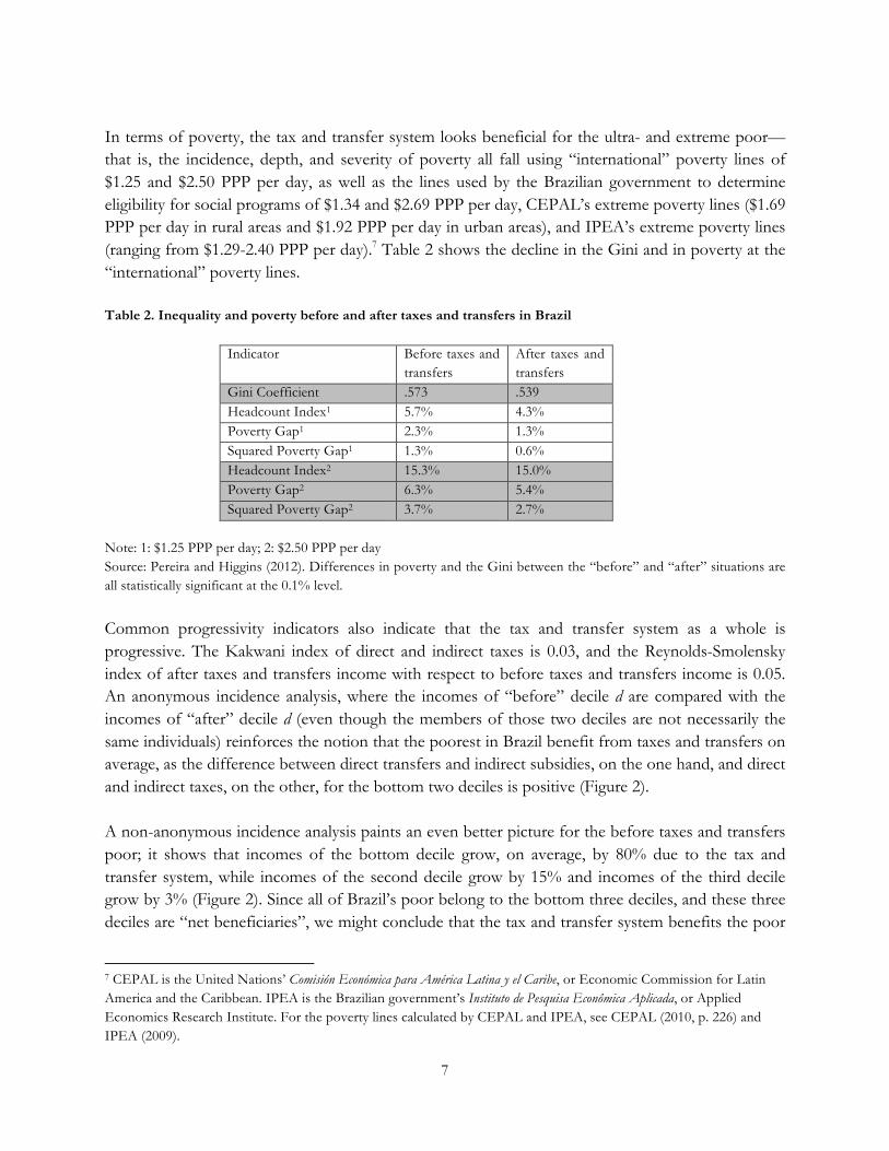
In terms of poverty, the tax and transfer system looks beneficial for the ultra- and extreme poor—that is, the incidence, depth, and severity of poverty all fall using “international” poverty lines of $1.25 and $2.50 PPP per day, as well as the lines used by the Brazilian government to determine eligibility for social programs of $1.34 and $2.69 PPP per day, CEPAL’s extreme poverty lines ($1.69 PPP per day in rural areas and $1.92 PPP per day in urban areas), and IPEA’s extreme poverty lines (ranging from $1.29-2.40 PPP per day).7 Table 2 shows the decline in the Gini and in poverty at the “international” poverty lines. Table 2. Inequality and poverty before and after taxes and transfers in Brazil

Indicator Before taxes and transfers

After taxes and transfers

Gini Coefficient .573 .539 Headcount Index1 5.7% 4.3% Poverty Gap1 2.3% 1.3% Squared Poverty Gap1 1.3% 0.6% Headcount Index2 15.3% 15.0% Poverty Gap2 6.3% 5.4% Squared Poverty Gap2 3.7% 2.7%

Note: 1: $1.25 PPP per day; 2: $2.50 PPP per day Source: Pereira and Higgins (2012). Differences in poverty and the Gini between the “before” and “after” situations are all statistically significant at the 0.1% level.

Common progressivity indicators also indicate that the tax and transfer system as a whole is progressive. The Kakwani index of direct and indirect taxes is 0.03, and the Reynolds-Smolensky index of after taxes and transfers income with respect to before taxes and transfers income is 0.05. An anonymous incidence analysis, where the incomes of “before” decile d are compared with the incomes of “after” decile d (even though the members of those two deciles are not necessarily the same individuals) reinforces the notion that the poorest in Brazil benefit from taxes and transfers on average, as the difference between direct transfers and indirect subsidies, on the one hand, and direct and indirect taxes, on the other, for the bottom two deciles is positive (Figure 2).

A non-anonymous incidence analysis paints an even better picture for the before taxes and transfers poor; it shows that incomes of the bottom decile grow, on average, by 80% due to the tax and transfer system, while incomes of the second decile grow by 15% and incomes of the third decile grow by 3% (Figure 2). Since all of Brazil’s poor belong to the bottom three deciles, and these three deciles are “net beneficiaries”, we might conclude that the tax and transfer system benefits the poor

7 CEPAL is the United Nations’ Comisión Económica para América Latina y el Caribe, or Economic Commission for Latin America and the Caribbean. IPEA is the Brazilian government’s Instituto de Pesquisa Econômica Aplicada, or Applied Economics Research Institute. For the poverty lines calculated by CEPAL and IPEA, see CEPAL (2010, p. 226) and IPEA (2009).

8

overall. However, this again ignores downward mobility among the poor. Even though this incidence analysis is non-anonymous (i.e., deciles are defined by before taxes and transfers income), the individual losers are masked by decile averages. Figure 2. Anonymous and non-anonymous fiscal incidence curves by deciles for Brazil

Source: Authors’ calculations based on POF (2008-2009).

In sum, taxes and transfers in Brazil reduce inequality and extreme poverty, are progressive and increase the incomes of the first two (three) deciles on average for the anonymous (non-anonymous) comparison.8 However, this resoundingly positive picture hides the fact that a non-trivial share of the non-poor/moderate poor/extreme poor become poor/extreme poor/ultra-poor, respectively.

Table 3 shows the transition matrix for Brazil—the fiscal mobility matrix P; the added last two rows and two columns show the population shares of each group and the mean income of members of that group. Our income groups in this example are six in total. The poor are divided into three groups: less than $1.25 PPP per day (the “ultra-poor”), between $1.25 and $2.50 PPP per day (the extreme poor), and between $2.50 and $4 PPP per day (the moderately poor). The three non-poor groups are: between $4 and $10 PPP per day (the vulnerable), between $10 and $50 PPP per day (the middle class), and above $50 PPP per day.9 As a result of indirect taxes,10 11 percent of those

8 These two curves are analogous to those used by Van Kerm (2009) in the context of growth. Also, see, Bourguignon (2011a). 9 The $1.25 PPP per day line approximately represents the average national poverty line of the bottom fifteen low-income, less-developed countries (Chen and Ravallion, 2010); thus in the context of middle-income Brazil we call those living on less than $1.25 PPP per day the “ultra poor”. The $2.50 and $4 PPP per day poverty lines are commonly used as extreme and moderate poverty lines for Latin America, and roughly correspond to the median official extreme and moderate poverty lines in those countries (CEDLAS and World Bank, 2010). The $10 PPP per day line is the upper bound of those vulnerable to falling into poverty in three Latin American countries, calculated by Lopez-Calva and Ortiz-Juarez (2011) and the lower bound of the middle class used by Kharas (2010) and Ferreira et al. (2012,

‐40%

‐20%

0%

20%

40%

60%

80%

100%

1 2 3 4 5 6 7 8 9 10

Increasewith

respecttoMarketIncom

e

Deciles

Non‐anonymous

Anonymous

9

vulnerable to poverty become poor, 15 percent of the moderate poor become extremely poor, and 4 percent of the extremely poor become ultra-poor despite any cash transfers they receive.11 As noted above, this downward mobility is not captured by the standard measures of inequality, poverty, progressivity, and incidence.

Table 3. Fiscal Mobility Matrix for Brazil Post-Fiscal Income groups

Market Income groups

y < 1.25 1.25 <= y < 2.50

2.50 <= y < 4.00

4.00 <= y < 10.00

10.00 <= y < 50.00

50.00 <= y

Percent of pop-ulation

Mean income

y < 1.25 69% 21% 6% 3% 5.7% $0.74

1.25 < = y < 2.50

4% 81% 10% 4% 9.6% $1.89

2.50 <= y < 4.00

15% 75% 9% 1% 11.3% $3.24

4.00 <= y < 10.00

11% 86% 3% 33.6% $6.67

10.00 <= y < 50.00

15% 85% 35.3% $19.90

50.00 <= y 32% 68% 4.5% $94.59

Percent of population

4.3% 10.7% 13.5% 35.8% 32.5% 3.2% 100% $14.15

Mean income

$0.86 $1.91 $3.25 $6.61 $19.34 $88.70 $12.17

Note: Mean incomes are in US$ PPP per day. Rows may not sum to exactly 100% due to rounding. Zeroes are omitted from the matrix for enhanced readability. Differences in group shares between the “before” and “after” scenarios are all statistically significant from zero at the 0.1% significance level. Source: Authors’ calculations based on POF (2008-2009).

While extreme poverty declines, moderate poverty increases when we compare the before and after taxes and transfers situations. Thus, comparing poverty indicators for moderate poverty would have alerted us to the downward mobility from the non-poor to the poor. In fact, in the presence of increased poverty, we can be assured of downward mobility. The problem is that, as we have shown for the extreme and ultra-poor, downward mobility can occur while poverty is reduced. An increase in poverty is thus a sufficient but not a necessary condition for downward mobility among the poor.

forthcoming). The $50 PPP per day line is the upper bound of the middle class proposed by Ferreira et al. (2012, forthcoming). 10 That this downward mobility is primarily a result of indirect rather than direct taxes can be shown a number of ways but will not be discussed further here; see Pereira and Higgins (2012) and Lustig (2011a). 11 Note that although some of the poor lose in terms of monetary income, tax revenues may benefit the poor in terms of access to public education, health and infrastructure, benefits that are not captured here.

10

Would checking for first-order stochastic dominance of the CDFs of before and after taxes and transfers income have alerted us to the downward mobility shown above? Graphing the CDFs of the “before” and “after” scenarios reveals that, over the entire income distribution, there is no weak first-order stochastic dominance; the two curves cross. Figure 2 graphs the CDFs up to $5 PPP per day (beyond that point the “before” situation lies always below the “after” situation; we choose this cut-off so that we can view the graph with sufficient detail). The dotted vertical lines represent our income group cutoffs: $1.25, $2.50, and $4 PPP per day. Note that the CDFs cross somewhere between $2.50 and $4 PPP per day. Thus, if we define everyone with income below $4 PPP per day as poor and define our poorest group as having income below $1.25 PPP per day, as we have above, we have no weak first-order stochastic dominance with the CDFs crossing to the left of the maximum poverty line and to the right of one of our income group cut-offs, which is a sufficient condition for downward mobility among the poor. Nevertheless, suppose instead that we considered those with income above $2.50 PPP per day as non-poor, and thus had two poor income groups: those with income less than $1.25 PPP per day and those with income between $1.25 and $2.50 PPP per day. In this case, the “after” situation exhibits strict first-order stochastic dominance over the “before” situation to the left of the poverty line, and hence we might conclude, even after checking for first order stochastic dominance, that the poor are better off after taxes and transfers. Again, we would be overlooking the fact that 4% of those with income between $1.25 and $2.50 PPP per day are becoming “ultra-poor” after taxes and transfers.

Figure 2. Cumulative distribution functions of “before” and “after” incomes in Brazil

Note: The y-axis is re-ranked by income concept. Source: Authors’ calculations based on POF (2008-2009).

This illustrates the importance of the fiscal mobility matrix: without it, we would be unable to identify downward fiscal mobility among the poor using standard indicators and analytical methods.

11

Now that we have established that taxes and transfers induce downward mobility among the poor, the next step is to ask how much the downwardly mobile poor lose. For this, we use the income loss matrix L, shown in Table 4. The income loss matrix shows us the average loss of losers, by their “before” and “after” income groups, as a proportion of their before taxes and transfers incomes. In addition, we include the average before taxes and transfers incomes of each of these groups. A couple of factors are striking. The ultra-poor who lose see their before transfer incomes—which begin at a meager $0.83 PPP per day, reduced by 10% on average. The extremely poor who become ultra-poor have before transfers income of $1.34 and lose 13% of their income on average. The moderately poor who become extremely poor have before transfers income of $2.71 PPP per day and lose 14% of their income on average.

Table 4. Income loss matrix for “losers” in Brazil Post-Fiscal Income groups

Market Income groups

y < 1.25 1.25 < = y < 2.50

2.50 <= y < 4.00

4.00 <= y < 10.00

10.00 <= y < 50.00

50.00 <= y

Percent of pop-ulation

Group average

y < 1.25 -10% $0.83

5.7% -10% $0.83

1.25 < = y < 2.50

-13% $1.34

-10% $2.01

9.6% -10% $1.96

2.50 <= y < 4.00

-14% $2.71

-11% $3.40

11.3% -11% $3.27

4.00 <= y < 10.00

-15% $4.36

-14% $7.04

33.6% -14% $6.70

10.00 <= y < 50.00

-16% $10.98

-16% $21.76

35.3% -16% $20.03

50.00 <= y -22% $56.66

-21% $113.30

4.5% -21% $94.99

Percent of population

4.3% 10.7% 13.5% 35.8% 32.5% 3.2% 100%

Group average

-11% $0.95

-11% $2.20

-12% $3.73

-14% $7.73

-16% $23.46

-21% $113.30

-14.5% $16.10

Note: All monetary amounts are using before taxes and transfers income and are in PPP-adjusted dollars per day. Zeroes are omitted from the matrix for enhanced readability. Differences in group shares between the “before” and “after” scenarios are all statistically significant from zero at the 0.1% significance level. Source: Authors’ calculations based on POF (2008-2009).

In sum, the fiscal mobility matrix and income loss matrix provide us with valuable information—that would not have been available using standard measures and techniques—about how many of the poor lose and how much they lose.

12

4. AN ALTERNATIVE SCENARIO FOR BRAZIL: A NEUTRAL TAX SYSTEM

Next, we might wish to compare the actual tax and transfer system to various counterfactual alternatives. These alternatives could ignore behavioral and general equilibrium effects or attempt to account for them; the one presented here will assume them away.

Consider the alternative of a “neutral tax” in which the government abolishes the current tax system but keeps tax revenue fixed at the current value by levying a tax on each individual proportional to their income. We call this a “neutral tax” because (ignoring behavioral and general equilibrium effects) it does not affect inequality—each individual is left with the same proportion of national income as they started with. In our counterfactual scenario, transfers remain equal to observed transfers received. The fiscal mobility matrix for this scenario is presented in Table 5, which can be compared to the actual scenario above (see Table 3).

Table 5. Fiscal Mobility Matrix for Counterfactual Neutral Tax in Brazil Post-Fiscal Income groups

Market Income groups

y < 1.25 1.25 < = y < 2.50

2.50 <= y < 4.00

4.00 <= y < 10.00

10.00 <= y < 50.00

50.00 <= y

Percent of population

Mean income

y < 1.25 69% 20% 7% 4% 1% 5.7% $0.74

1.25 < = y < 2.50

7% 78% 9% 5% 1% 9.6% $1.89

2.50 <= y < 4.00

22% 67% 9% 1% 11.3% $3.24

4.00 <= y < 10.00

16% 81% 3% 33.6% $6.67

10.00 <= y < 50.00

19% 81% 35.3% $19.90

50.00 <= y 29% 71% 4.5% $94.59

Percent of population

4.7% 11.1% 14.2% 35.4% 31.3% 3.3% 100% $14.15

Mean income

$0.86 $1.90 $3.25 $6.61 $19.40 $91.54 $12.17

Note: Mean incomes are in US$ PPP per day. Rows may not sum to exactly 100% due to rounding. Zeroes are omitted from the matrix for enhanced readability. Differences in group shares between the “before” and “after” scenarios are all statistically significant from zero at the 0.1% significance level. Source: Authors’ calculations based on POF (2008-2009). It is easy to see that there is higher downward mobility among the poor in the neutral tax scenario than in the actual case: for row 2, the actual downward mobility vector (.04) < the neutral tax downward mobility vector (.07). For row 3, the actual cumulative downward mobility vector (0, .15) < the neutral tax cumulative downward mobility vector (0, .22). For row 4, the actual cumulative downward mobility vector (0, 0, .11) < the neutral tax cumulative downward mobility vector (0, 0,

13

.16). For rows 4, 5, and 6, there is no downward mobility into columns � ≤ � = 3, so the downward mobility vectors for those rows are equal. Formally, there is strong downward mobility dominance (as defined in Section 2) of the actual scenario over the neutral tax. Thus, we can conclude that a neutral tax would be detrimental to a large portion of the poor.

In addition to alternative tax scenarios, the government could consider attempting to compensate the losing poor for their losses, and to prevent any non-poor from becoming poor (by compensating them up to the point that they remain non-poor). The cost of this would amount to about $6.5 billion reais per year; to put this amount in perspective, it is 0.2% of GDP, or around half the total transfers paid by Bolsa Família. Of course, this amount underestimates the true cost of offsetting downward fiscal mobility among the poor, as it assumes perfect knowledge about who is losing and how much they are losing; nevertheless, it can be thought of as a lower bound of the cost of preventing downward mobility among the poor.

5. CONCLUDING REMARKS

We have shown that a country can perform well by standard indicators of inequality, poverty, first order stochastic dominance, fiscal incidence, and progressivity despite having a non-trivial sub-section of the poor experience downward fiscal mobility into a lower income group (and having a non-trivial sub-section of the non-poor experience downward mobility into poverty). Anonymous indicators, such as the Gini, headcount, poverty gap, and squared poverty gap indices, overlook downward fiscal mobility among the poor because they do not concern themselves with who the before transfers poor are. Fiscal mobility matrices are a useful tool for identifying how much downward fiscal mobility occurs among the poor. In the case of Brazil we saw that 11 percent of the non-poor become poor, 15 percent of the moderate poor become extremely poor, and 4 percent of the extremely poor become ultra-poor despite any cash transfers they receive. Meanwhile, we would not have been aware of this downward fiscal mobility if we relied on standard tools; extreme poverty and inequality declines, there is first order stochastic dominance to the left of the $2.50 PPP per day line, and taxes and transfers are progressive and increase the incomes of the poorest deciles.

14

REFERENCES

Bourguignon, Francois. 2011a. “Non-Anonymous Growth Incidence Curves, Income Mobility and Social Welfare Dominance,” Journal of Economic Inequality 9(4): 605-627. Bourguignon, François. 2011b. “Status Quo in the Welfare Analysis of Tax Reforms.” Review of

Income and Wealth 57(4): 603-621. Chakravarty, Satya, Nora Lustig, Nachiketa Chattopadhyay and Sean Higgins. 2012. “Directional

Movement and Welfare Dominance in Alternative States,” mimeo, work in progress. CEDLAS (Centro de Estudios Distributivos, Laborales y Sociales) and World Bank. 2010. “A Guide

to the SEDLAC Socio-Economic Database for Latin America and the Caribbean.” http://www.depeco.econo.unlp.edu.ar/cedlas/sedlac/pdfs/guide_sedlac.pdf

Chen, Shaohua and Martin Ravallion. 2010. “The Developing World is Poorer than We Thought, but No Less Successful in the Fight Against Poverty.” The Quarterly Journal of Economics 125(4): 1577-1625.

Ferreira, Francisco, Julián Messina, Jamele Rigolini and Renos Vakis. 2012 (forthcoming). Socio-Economic Mobility and the Rise of the Middle Class in Latin America and the Caribbean. World Bank Regional Flagship Report for Latin America and the Caribbean.

Fields, Gary S. 2008. “Income mobility.” In The New Palgrave Dictionary of Economics, Second Edition, edited by Lawrence Blume and Stephen Durlauf.

Kharas, Homi. 2010. “The Emerging Middle Class in Developing Countries.” OECD Development Centre Working Paper 285. http://www.oecd.org/dataoecd/12/52/44457738.pdf

Lopez-Calva, Luis F. and Ortiz-Juarez, Eduardo. 2011. “A Vulnerability Approach to the Definition of the Middle Class.” Policy Research Working Paper 5902. Washington, D.C.: World Bank.

Lustig, Nora (coordinator). 2011a. “Fiscal Policy, ‘Fiscal Mobility,’ the Poor, the Vulnerable and the Middle Class in Latin America.” Argentina (Carola Pessino), Bolivia (George Gray-Molina, Wilson Jimenez, Veronica Paz and Ernesto Yañez), Brazil (Claudiney Pereira and Sean Higgins) and Peru (Miguel Jaramillo. Background paper for World Bank, Vicepresidency for Latin America and the Caribbean “From Opportunity to Achievement: Socioeconomic Mobility and the Rise of the Middle Class in Latin America.

___________. 2011b. Fiscal Policy and Income Redistribution in Latin America: Challenging the Conventional Wisdom. Argentina (Carola Pessino), Bolivia (George Gray-Molina, Wilson Jimenez, Veronica Paz and Ernesto Yañez), Brazil (Claudiney Pereira and Sean Higgins), Mexico (John Scott) and Peru (Miguel Jaramillo), Working Paper, Tulane University.

___________. 2011c. “Commitment to Equity Assessment (CEQ) A Diagnostic Framework to Assess Governments’ Fiscal Policies Handbook.” Working Paper No. 1119, Dept. of Economics, Tulane University, April. http://econ.tulane.edu/RePEc/pdf/tul1119.pdf

Pereira, Claudiney and Sean Higgins. 2012. “Fiscal Policy, Urban-Rural Inequality and Rural Poverty in Brazil.” Report prepared for the International Fund for Agricultural Development.

Van Kerm, Philippe. 2009. “Income Mobility Profiles.” Economics Letters 102(2): 93-95.

15

CEQ WORKING PAPER SERIES “Commitment to Equity Assessment (CEQ): Estimating the Incidence of Social Spending, Subsidies

and Taxes. Handbook,” by Nora Lustig and Sean Higgins, CEQ Working Paper No. 1, July 2011; revised January 2013.

“Commitment to Equity: Diagnostic Questionnaire,” by Nora Lustig, CEQ Working Paper No. 2, 2010; revised August 2012.

“The Impact of Taxes and Social Spending on Inequality and Poverty in Argentina, Bolivia,Brazil, Mexico and Peru: A Synthesis of Results,” by Nora Lustig, George Gray Molina, Sean Higgins, Miguel Jaramillo, Wilson Jiménez, Veronica Paz, Claudiney Pereira, Carola Pessino, John Scott, and Ernesto Yañez, CEQ Working Paper No. 3, August 2012.

“Fiscal Incidence, Fiscal Mobility and the Poor: A New Approach,” by Nora Lustig and Sean Higgins, CEQ Working Paper No. 4, September 2012.

“Social Spending and Income in Argentina in the 2000s: the Rising Role of Noncontributory Pensions,” by Nora Lustig and Carola Pessino, CEQ Technical Paper No. 5, January 2013.

“Explaining Low Redistributive Impact in Bolivia,” by Verónica Paz Arauco, George Gray Molina, Wilson Jiménez Pozo, and Ernesto Yáñez Aguilar, CEQ Working Paper No. 6, January 2013.

“The Effects of Brazil’s High Taxation and Social Spending on the Distribution of Household Income,” by Sean Higgins and Claudiney Pereira, CEQ Working Paper No.7, January 2013.

“Redistributive Impact and Efficiency of Mexico’s Fiscal System,” by John Scott, CEQ Working Paper No. 8, January 2013.

“The Incidence of Social Spending and Taxes in Peru,” by Miguel Jaramillo Baanante, CEQ Working Paper No. 9, January 2013.

“Social Spending, Taxes, and Income Redistribution in Uruguay,” by Marisa Bucheli, Nora Lustig, Máximo Rossi and Florencia Amábile, CEQ Working Paper No. 10, January 2013.

“Social Spending, Taxes and Income Redistribution in Paraguay,” Sean Higgins, Nora Lustig, Julio Ramirez (CADEP), Billy Swanson, CEQ Working Paper No. 11, February 2013.

16

The CEQ logo is a stylized graphical representation of a Lorenz curve for a fairly unequal distribution of income (the bottom part of the C, below the diagonal) and a concentration curve for a very progressive transfer (the top part of the C).

What is CEQ?

Led by Nora Lustig (Tulane University) and Peter Hakim (Inter-American Dialogue), the Commitment to Equity (CEQ) project is designed to analyze the impact of taxes and social spending on inequality and poverty, and to provide a roadmap for governments, multilateral institutions, and nongovernmental organizations in their efforts to build more equitable societies. CEQ/Latin America is a joint project of the Inter-American Dialogue (IAD) and Tulane University’s Center for Inter-American Policy and Research (CIPR) and Department of Economics. The project has received financial support from the Canadian International Development Agency (CIDA), the Development Bank of Latin America (CAF), the General Electric Foundation, the Inter-American Development Bank (IADB), the International Fund for Agricultural Development (IFAD), the Norwegian Ministry of Foreign Affairs, the United Nations Development Programme’s Regional Bureau for Latin America and the Caribbean (UNDP/RBLAC), and the World Bank. http://commitmenttoequity.org