Kalman Filter Based Algorithms for Fast Training of Multilayer Perceptrons: Implementation and Applications

ECE 539 Project

• Dan Li• Spring, 2000

IntroductionIntroduction

• Multilayer perceptron (MLP) – A feedforward neural network model– Extensively used in pattern classification– Essential issue: training/learning algorithm

• MLP training algorithms– Error backpropogation (EBP)

• A conventional iterative gradient algorithm• Easy to implement• Long and uncertain training process

– An algorithm proposed by Scalero and Tepedelenlioglu [1]: S.T. Algorithm (based on Kalman filter techniques)

– Modified S.T. algorithm proposed by Wang and Chen [2] : Layer-by-layer (LBL) Algorithm (based on Kalman filter techniques)

EBP AlgorithmEBP Algorithm

x1

x2

xM

1

1

Fh(.)

Fh(.)

Fh(.)

Fo(.)

Fo(.)

Fo(.)

u1

u2

uH

y1

y2

yH

z1

z2

zN

v1

v2

vH

.

.

.

.

.

.

.

.

.

.

.

.

.

.

.

.

.

.

N

k

Okj

Okjh

Hj

Hji

Hji

Hj

Hji

Hji

nwnnuFn

nwnwnnwnw

1

)()(')(

)()()()()(

)()())(()(

)]1()([)()()1(

)]()([))(()(

)]1()([)()()1(')(

)()()()()(

nzntnvFn

nwnwnnwnw

jjjooj

oji

oji

oj

oji

oji

For the hidden layer For the output layer

S.T. AlgorithmS.T. Algorithm

x1

x2

xM

1

1

Fh(.)

Fh(.)

Fh(.)

Fo(.)

Fo(.)

Fo(.)

u1

u2

uH

y1

y2

yH

z1

z2

zN

F-1o(.)

t1

t2

tN

F-1o(.)

F-1o(.)

v1

v2

vN

-+

ev1

*

-+

e

-+

e

v2*

vN*

-+

e

-+

e

-+

e

u1*

u2*

uM*

.

.

....

.

.

.

.

.

.

.

.

.

.

.

.

For the hidden layer For the output layer

)()())(()(

)())(())(()(

)()()1()(

')(

)()(')(

)()()(

nzntnvFn

nwnnuFn

nknnwnw

jjjooj

Oj

Tojh

Hj

HHj

Hj

Hj

)())(()()()(

)()()1()(1*

)()(

nvntFnvnvne

nenknwnw

jjojjj

jooj

oj

LBL AlgorithmLBL Algorithm

x1

x2

xM

1

Fh()

Fh()

Fh()

Fo()

Fo()

Fo()

u1

u2

uH

y1

y2

yH

z1

z2

zN

F-1o()

t1

t2

tN

F-1o()

F-1o()

v1

v2

vN

-+

ev1

*

-+

e

-+

e

v2*

vN*

-+

e

F-1h()

F-1h()

F-1h()

-+

e

-+

e

u1*

u2*

uN*

y1*

y2*

yH*

1

.

.

.

.

.

....

.

.

....

.

.

.

For the hidden layer For the output layer

)()1())(()()()(

)()()1()(*1* nxnWnyFnunune

nenknWnW

ohH

THHHH

)1()1())1(()1()1()1(

)1()()1()(1*

nnWntFnvnvne

nenknWnW

ooo

Toooo

Experiment #1: 4-4 Encoding/DecodingExperiment #1: 4-4 Encoding/Decoding

0 0 0 0 0 0 0 00 0 0 1 0 0 0 10 0 1 0 0 0 1 00 0 1 1 0 0 1 10 1 0 0 0 1 0 00 1 0 1 0 1 0 10 1 1 0 0 1 1 00 1 1 1 0 1 1 11 0 0 0 1 0 0 01 0 0 1 1 0 0 11 0 1 0 1 0 1 01 0 1 1 1 0 1 11 1 0 0 1 1 0 01 1 0 1 1 1 0 11 1 1 0 1 1 1 01 1 1 1 1 1 1 1

Input Target

0 200 400 600 800 10001

1.5

2

2.5

3

3.5

4

4.5Learning Curve

Epoch

MSEEBP

S.T.

LBL

      

# of Epochs CPU time (sec) Learning error Correct rate

EBP 1000 73.906 >1.4 62.50%S.T. 1000 85.473 >1.4 75%LBL 42 4.164 1.2 87.50%

• MLP Structure: 4-3-4; =0.16 • EBP: =0.3; =0.8; S.T.: =0.3; H= o=0.9; LBL: =0.15; H= o=0.9;

Experiment #2: Pattern Classification (IRIS)Experiment #2: Pattern Classification (IRIS)

      

4 input features3 classes (001, 010, 100)75 training patterns75 testing patterns

0 200 400 600 8000

1

2

3

4

5

6Learning Curve

EpochM

SE

EBP S.T.

# of epochs CPU time (s) Correct rate (Training) Correct rate (Testing)

EBP 800 339.178 96.00% 88.00%S.T. 800 393.045 98.67% 93.33%

• MLP Structure: 4-3-3; =0.01• EBP: =0.3; =0.8; S.T.: =20; H= o=0.9;

Experiment #3: Pattern Classification (wine)Experiment #3: Pattern Classification (wine)

13 input features3 classes (001, 010, 100)60 training patterns118 testing patterns

• MLP Structure: 13-15-3; • EBP: =0.3; =0.8; S.T.: =20; H= o=0.9; LBL: =0.2; H= o=0.9;

0 100 200 300 400 5000

1

2

3

4

5

6

7Learning Curve

EpochM

SE

EBP

LBL

S.T.

# of epochs CPU time (s) Correct rate (Training) Correct rate (Testing)

EBP 500 201.469 30.00% 27.97%S.T. 500 254.156 100.00% 70.34%LBL 500 301.814 55.00% 48.33%

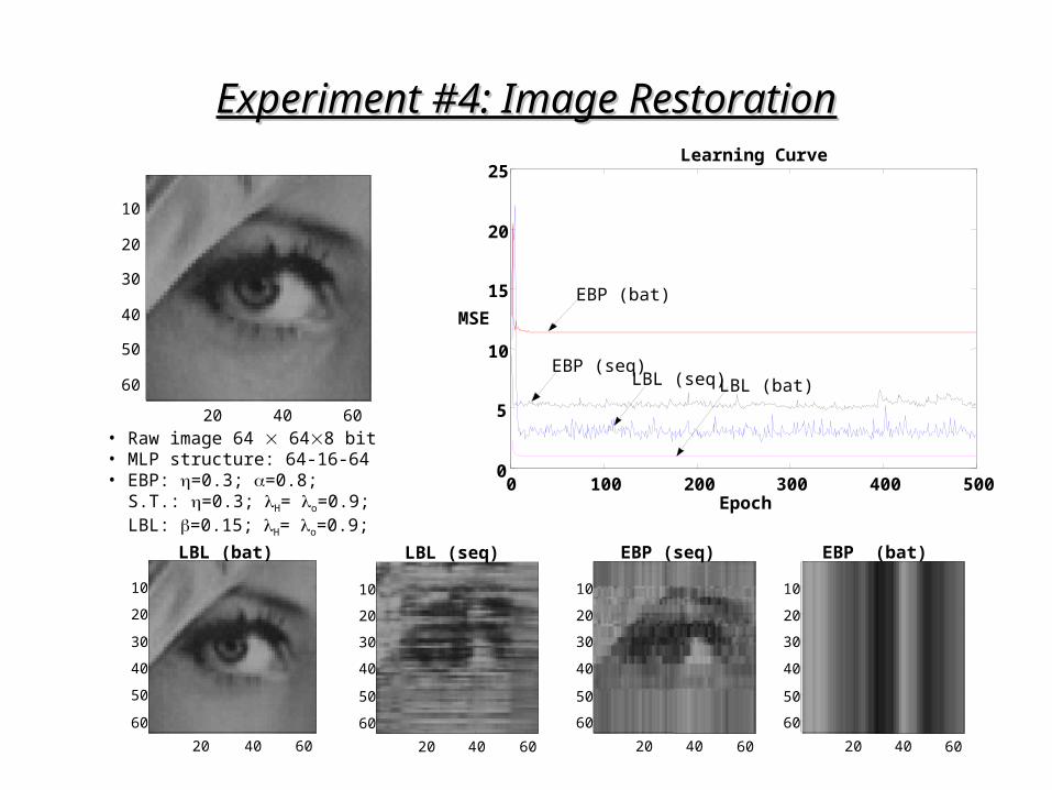
Experiment #4: Image RestorationExperiment #4: Image Restoration

20 40 60

10

20

30

40

50

60

0 100 200 300 400 5000

5

10

15

20

25Learning Curve

Epoch

MSEEBP (bat)

EBP (seq) LBL (seq) LBL (bat)

• Raw image 64 648 bit • MLP structure: 64-16-64• EBP: =0.3; =0.8; S.T.: =0.3; H= o=0.9; LBL: =0.15; H= o=0.9;

20 40 60

10

20

30

40

50

60

LBL (bat)

20 40 60

10

20

30

40

50

60

LBL (seq)

20 40 60

10

20

30

40

50

60

EBP (bat)

20 40 60

10

20

30

40

50

60

EBP (seq)

Experiment #5: Image Reconstruction Experiment #5: Image Reconstruction (I)(I)

Original Image(2562568 bit)

* Schemes of selecting training subsets (shaded area)

11

32

256

32 256 11

64

256

64 256A 32 input features B 64 input features

Experiment #5: Image Reconstruction Experiment #5: Image Reconstruction (II)(II)

Epoch

0 50 100 150 2000

10

20

30

40

50

60

MS

E

EBP (bat)

LBL (bat) LBL (seq) EBP (seq)

Restored: LBL (bat) Restored: LBL (seq) Restored: EBP (seq)

• MLP structure: 32-16-32• Convergence threshold: MSE=5• EBP: =0.3; =0.8; LBL: =0.15; H= o=0.9;

Scheme A

# of epchs CPU time

EBP (seq) 200 1237.789EBP(bat) 200 66.806LBL (seq) 200 2406.661LBL (bat) 7 4.376

0 50 100 150 2000

10

20

30

40

50

60

70

80

90

Epoch

MS

E

EBP (bat)

EBP (seq)

LBL (bat) LBL (seq)

Restored: LBL (bat) Restored: LBL (seq) Restored: EBP (seq)

Experiment #5: Image Reconstruction Experiment #5: Image Reconstruction (III)(III)

• MLP structure: 64-32-64• Convergence threshold: MSE=5• EBP: =0.3; =0.8; LBL: =0.15; H= o=0.9;

# of epchs CPU time

EBP (seq) 200 2587.361EBP(bat) 200 166.039LBL (seq) 200 7058.199LBL (bat) 6 9.123

Scheme B

Experiment #5: Image Reconstruction Experiment #5: Image Reconstruction (IV)(IV)

Restored: LBL (seq)Restored: S.T. (seq)Restored: EBP (seq)

0 20 40 60 80 1000

10

20

30

40

50

60

70

80

Epoch

MS

E

ST (seq) EBP (seq) EBP (seq) LBL (seq)

LBL (bat) EBP (bat)

Scheme A, Noisy Image for Training

• MLP structure: 32-16-32• Convergence threshold: MSE=5• EBP: =0.3; =0.8; LBL: =0.15; H= o=0.9;

ConclusionsConclusions

• Compared with EBP algorithm, Kalman-filter-based S.T. and LBL algorithms generally induce a lower MSE in the training process in a significantly smaller number of epochs.

• However, the CPU time needed to run one iteration is longer for the S.T. and LBL algorithms, due to the computation of Kalman gain, the inverse of correlation matrices and the (pseudo)inverse of the output in each layer. LBL often required even longer computation time than the S.T. algorithm.

• Therefore, the total computation time required is determined by the user’s demand: how well the training result would you like? This is in fact the issue of assigning the “convergence threshold of MSE”. Our examples showed that in various applications, the choice of this threshold generally results a shorter overall training time for the Kalman-filter-based method than for the EBP method.

• There is no definite answer to the question “which algorithm converges faster, the LBL or the S.T.?”. Essentially it is case-related. Especially in the S.T. algorithm, the learning rate has a more flexible range not bounded to [0, 1], in contrast to the EBP algorithm.

ReferencesReferences

1. Robert S. Scalero and Nazif Tepedelenlioglu, “A fast new algorithm for training feedforward neural networks”, IEEE Transactions on Signal Processing, Vol. 40, No. 1, pp. 202-210, 1992.

2. Gou-Jen Wang and Chih-Cheng Chen, “A fast multilayer neural-network training algorithm based on the layer-by-layer optimizing procedures”, IEEE Transactions on Neural Networks, Vol. 7, No. 3, pp. 768-775, 1996.

3. Brijesh Verma, “Fast training of multilayer perceptrons”, IEEE Transactions on Neural Networks, Vol. 8, No. 6, pp. 1314-1320, 1997.

4. Adriana Dumitras and Vasile Lazarescu, “The influence of the MLP’s output dimension on its performance in image restoration”, ISCAS ’96, Vol. 1, pp. 329-332