First-principle calculations of the Berry curvature of ... · First-principle calculations of the...

First-principle calculations of the Berry curvature of Bloch states for charge and spin transport

of electrons

This article has been downloaded from IOPscience. Please scroll down to see the full text article.

2012 J. Phys.: Condens. Matter 24 213202

(http://iopscience.iop.org/0953-8984/24/21/213202)

Download details:

IP Address: 160.45.66.65

The article was downloaded on 16/10/2012 at 13:16

Please note that terms and conditions apply.

View the table of contents for this issue, or go to the journal homepage for more

Home Search Collections Journals About Contact us My IOPscience

http://iopscience.iop.org/page/terms

http://iopscience.iop.org/0953-8984/24/21

http://iopscience.iop.org/0953-8984

http://iopscience.iop.org/

http://iopscience.iop.org/search

http://iopscience.iop.org/collections

http://iopscience.iop.org/journals

http://iopscience.iop.org/page/aboutioppublishing

http://iopscience.iop.org/contact

http://iopscience.iop.org/myiopscience

IOP PUBLISHING JOURNAL OF PHYSICS: CONDENSED MATTER

J. Phys.: Condens. Matter 24 (2012) 213202 (23pp) doi:10.1088/0953-8984/24/21/213202

TOPICAL REVIEW

First-principle calculations of the Berrycurvature of Bloch states for charge andspin transport of electrons

M Gradhand1,2, D V Fedorov1,3, F Pientka3,4, P Zahn3,5, I Mertig1,3 andB L Gyorffy2

1 Max Planck Institute of Microstructure Physics, Weinberg 2, 06120 Halle, Germany2 H H Wills Physics Laboratory, University of Bristol, Bristol BS8 1TH, UK3 Institute of Physics, Martin Luther University Halle-Wittenberg, 06099 Halle, Germany4 Dahlem Center for Complex Quantum Systems and Fachbereich Physik, Freie Universitat Berlin,14195 Berlin, Germany5 Institute of Ion Beam Physics and Materials Research, Helmholtz-Zentrum Dresden-Rossendorf e.V.,PO Box 510119, 01314 Dresden, Germany

E-mail: [email protected]

Received 15 February 2012, in final form 3 April 2012Published 11 May 2012Online at stacks.iop.org/JPhysCM/24/213202

AbstractRecent progress in wave packet dynamics based on the insight of Berry pertaining to adiabaticevolution of quantum systems has led to the need for a new property of a Bloch state, theBerry curvature, to be calculated from first principles. We report here on the response to thischallenge by the ab initio community during the past decade. First we give a tutorialintroduction of the conceptual developments we mentioned above. Then we describe fourmethodologies which have been developed for first-principle calculations of the Berrycurvature. Finally, to illustrate the significance of the new developments, we report someresults of calculations of interesting physical properties such as the anomalous and spin Hallconductivity as well as the anomalous Nernst conductivity and discuss the influence of theBerry curvature on the de Haas–van Alphen oscillation.

(Some figures may appear in colour only in the online journal)

Contents

1. Introduction: semiclassical electronic transport insolids, wave packet dynamics, and the Berrycurvature 21.1. New features of the Boltzmann equation 21.2. Berry phase, connection and curvature of Bloch

electrons 31.3. Abelian and non-Abelian curvatures 41.4. Symmetry, topology, codimension and the

Dirac monopole 51.5. The spin polarization gauge 6

2. First-principle calculations of the Berry curvature forBloch electrons 82.1. KKR method 82.2. Tight-binding model 102.3. Wannier interpolation scheme 132.4. Kubo formula 15

3. Intrinsic contribution to the charge and spinconductivity in metals 17

4. De Haas–van Alphen oscillation and the Berry phases 205. Conclusion 21

Acknowledgments 22References 22

10953-8984/12/213202+23$33.00 c© 2012 IOP Publishing Ltd Printed in the UK & the USA

http://dx.doi.org/10.1088/0953-8984/24/21/213202

mailto:[email protected]

http://stacks.iop.org/JPhysCM/24/213202

J. Phys.: Condens. Matter 24 (2012) 213202 Topical Review

1. Introduction: semiclassical electronic transport insolids, wave packet dynamics, and the Berrycurvature

Some recent, remarkable advances in the semiclassicaldescription of charge and spin transport by electrons insolids motivate a revival of interest in a detailed k-point byk-point study of their band structure. A good summary ofthe conceptual developments and the experiments they havestimulated has been given by Di Xiao et al [1]. Here wewish to review only the role and prospects of first-principleelectronic structure calculations in this rapidly moving field.

1.1. New features of the Boltzmann equation

Classically, particle transport is considered to take place inphase space, whose points are labeled by the position vectorr and the momentum p, and is described by the distributionfunction f (r,p, t), which satisfies the Boltzmann equation.Electrons in solids fit into this framework if we view theparticles as wave packets constructed from the Bloch waves,9nk (r) = eik·run(r,k), eigenfunctions of the unperturbedcrystal Hamiltonian H0 with band index n and the dispersionrelation Enk. If such a wave packet is strongly centered atkc in the Brillouin zone, it predominantly includes Blochstates with quantum numbers k close to kc and the particlecan be said to have a momentum hkc. Then, if we call itsspatial center rc its position, the transport of electrons canbe described by an ensemble of such quasiparticles. One ofthem is described by the distribution function fn(rn

c,knc, t).

For simplicity, the band index n is dropped in the followingfor f , rc, and kc. As f (rc,kc, t) evolves in phase space, theusual form of the Boltzmann equation, which preserves thetotal probability, is given by

∂tf + rc ·∇rc f + kc ·∇kc f =

(δf

δt

)scatt

. (1)

Here the first term on the left hand side is the derivative withrespect to the explicit time dependence of f , the next twoterms account for the time dependence of rc and kc, and theterm on the right-hand side describes the scattering of electronstates, by defects and other perturbations, in and out of theconsidered phase space volume centered at rc and kc. Thetime evolution of rc(t) and kc(t) is given by semiclassicalequations of motion, which in the presence of external electricE and magnetic B fields take conventionally the followingform:

rc =1h

∂Enk

∂k

∣∣∣∣k=kc

= vn(kc), (2)

hkc = −eE− erc × B. (3)

Here, the group velocity vn(kc) involves the unperturbedband structure. In the presence of a constant electric E =(Ex, 0, 0) and magnetic B= (0, 0,Bz) field, the solution of theabove equations yields the Hall resistivity ρxy ∝ Bz. However,for a ferromagnet with magnetization M = (0, 0,Mz)

the above theory cannot account for the experimentally

observed (additional) anomalous contribution ρxy ∝ Mz. Fora necessary correction of the theory, one needs to construct awave packet [2]

Wkc,rc(r, t) =∑

k

ak(kc, t)9nk(r), (4)

carefully taking into account the phase of the weightingfunction ak(kc, t). Requiring the wave packet to becentered at rc = 〈Wkc,rc |r|Wkc,rc〉 and considering zeroorder in the magnetic field only, it follows that ak(kc, t) =|ak(kc, t)|ei(k−kc)·An(kc)−ik·rc [2], where

An(kc) = i∫

u.c.d3r u∗n(r,kc)∇kun(r,kc) (5)

is the Berry connection, as will be discussed in detail insection 1.2. Note that the integral is restricted to only one unitcell (uc). Now, using the wave packet of equation (4), one canconstruct the Lagrangian

L(t) = 〈W| ih∂t − H |W〉 (6)

and minimize the action functional S[rc(t),kc(t)] =∫ tdt′L(t′)

with respect to arbitrary variations in rc(t) and kc(t).This maneuver replaces the quantum mechanical expectationvalues with respect to Wkc,rc(r, t) by the classical equationsof motion for rc(t) and kc(t). From the Euler–Lagrangeequations

ddt

∂L

∂kc−∂L

∂kc= 0 and

ddt

∂L

∂ rc−∂L

∂rc= 0, (7)

one gets

rc =1h

∂Enk

∂k|k=kc − kc ×Ωn (kc) , (8)

hkc = −eE− erc × B. (9)

Here Ωn(kc) is the so-called Berry curvature, defined as

Ωn(kc) = ∇k × An(k)|k=kc , (10)

the main subject of this review. For simplicity, several furtherterms in equations (8) and (9) were neglected. These are fullydiscussed in [1, 2]. For the purpose of this review the aboveform is sufficient to highlight the occurrence of the Berrycurvature in the equations of motion.

In comparison to equation (2), the new equation ofmotion for rc(t) given by equation (8) has an additional termproportional to the electric field called the anomalous velocity

van(kc) =

e

hE×Ωn (kc) . (11)

The presence of this velocity provides the anomalouscontribution to the Hall current jHy = jH,↑y + jH,↓y , where thespin-resolved currents may be written as

jH,↑y = −e∫

BZ

d3kc

(2π)3ry

c↑(kc)f↑(kc) = σ↑yx(Mz)Ex. (12)

jH,↓y = −e∫

BZ

d3kc

(2π)3ry

c↓(kc)f↓(kc) = σ↓yx(Mz)Ex. (13)

2


Figure 1. (a) The anomalous Hall effect and (b) the spin Hall effect.

In this notation f↑(kc) and f↓(kc) are the spin-resolveddistribution functions which are solutions of equation (1).Here rc and t are dropped due to homogeneous andsteady state conditions. In the limit of no scattering theyreduce to the equilibrium distribution functions and only theintrinsic mechanism, governed by the anomalous velocity ofequation (11), contributes to the Hall component. In general,jH,↑y and jH,↓y have opposite signs because of rc↓(kc) andrc↑(kc). However, the resulting charge current is nonvanishing(see figure 1(a)) due to the fact that the numbers of spin-upand spin-down electrons differ in ferromagnets with a finitemagnetization M 6= 0. In contrast to the anomalous Hall effect(AHE) in ferromagnets, the absence of the magnetizationin normal metals leads to the presence of time inversionsymmetry and, as a consequence, jH,↑y =−jH,↓y . This implies avanishing charge current, i.e. Hall voltage, but the existence ofa pure spin current as depicted in figure 1(b), which is knownas the spin Hall effect (SHE).

1.2. Berry phase, connection and curvature of Blochelectrons

Here we introduce briefly the concept of such relatively novelquantities as the Berry phase, connection, and curvature whicharise in the case of an adiabatic evolution of a system.

1.2.1. Adiabatic evolution and the Berry phase. Let usconsider an eigenvalue problem of the following form:

H(r, λ1, λ2, λ3)8n(r; λ1, λ2, λ3)

= En(λ1, λ2, λ3)8n(r; λ1, λ2, λ3), (14)

where H is a differential operator, 8n and En are the ntheigenfunction and eigenvalue, respectively, the vector r isa variable, and λ1, λ2, λ3 are parameters. A mathematicalproblem of general interest is the way such eigenfunctionschange if the set λ = (λ1, λ2, λ3) changes slowly withtime. If it is assumed that the process is adiabatic, thatis to say there is no transition from one to another state,then for a long time it was argued that a state 8n(r, λ, t)evolves in time as 8n(r, λ, t) = 8n(r, λ) exp(− i

h

∫ t0 dt′En

(λ1(t′), λ2(t′), λ3(t′)) + iγn(t)), where the phase γn(t) ismeaningless as it can be gauged away. In 1984 Berry [3]discovered that, while this is true for an arbitrary open pathin the parameter space, for a path that returns to the startingvalues λ1(0), λ2(0), and λ3(0) the accumulated phase isgauge invariant and is therefore a meaningful and measurable

Figure 2. A closed path in the parameter space.

quantity. In particular, he showed that for a closed path,labeled C in figure 2, the phase γn, called the Berry phasetoday, can be described by a line integral as

γn =

∮C

dλ ·An(λ), (15)

where the connection An(λ) is given by

An(λ) = i∫

d3r 8∗n(r, λ)∇λ8n(r, λ). (16)

The surprise is that, although the connection is not gaugeinvariant, γn and even more interestingly the curvature

Ωn(λ) = ∇λ × An(λ) (17)

are. As will be shown presently, these ideas are directlyrelevant for the dynamics of wave packets in the transporttheory discussed above.

1.2.2. Berry connection and curvature for Bloch states.Somewhat surprisingly, the above discussion has a numberof interesting things to say about the wave packets in thesemiclassical approach for spin and charge transport ofelectrons in crystals. Its relevance becomes evident if we takethe Schrodinger equation for the Bloch state(

−h2

2m∇

2r + V(r)

)9nk(r) = Enk9nk(r) (18)

3


and rewrite it for the periodic part of the Bloch function(−

h2

2m(∇r + ik)2 + V(r)

)un(r,k) = Enkun(r,k). (19)

The point is that the differential equation for 9nk(r), asimultaneous eigenfunction of the translation operator and theHamiltonian, does not depend on the wave vector, since k onlylabels the eigenvalues of the translation operator. However, inequation (19) k appears as a parameter and hence the abovediscussion of the Berry phase, the corresponding connection,and curvature applies directly to the periodic part of thewave function un(r,k). In short, for each band n there is aconnection associated with every k given by

An(k) = i∫

ucd3r u∗n(r,k)∇kun(r,k). (20)

Furthermore, the curvature

Ωn(k) = ∇k × An(k)

= i∫

ucd3r∇ku∗n(r,k)×∇kun(r,k) (21)

is the quantity that appears in the semiclassical equationof motion for the wave packet in equation (8). Thus,the curvature and the corresponding anomalous velocity inequations (11) associated with the band n are properties ofun(r,k). To emphasize this point, we note that the Blochfunctions 9nk(r) are orthogonal to each other

〈9nk|9n′k′〉 =

∫crystal

d3r 9∗nk(r)9n′k′(r) = δk,k′δn,n′ , (22)

and hence k is not a parameter. In contrast, un(r,k) isorthogonal to un′(r,k) but not necessarily to un(r,k′), as thisis an eigenfunction of a different Hamiltonian.

The observation that the above connection and curvatureare properties of the periodic part of the Bloch functionprompts a further comment. Note that for vanishing periodicpotential the Bloch functions would reduce to plane waves.Constructing the wave packet from plane waves meansun(r,k) = 1. Evidently, this means that Ωn(k) and An(k)vanish, and this fact is consistent with the general notion thatthe connection and the curvature arise from including onlyone or in any case a finite number of bands in constructingthe wave packet. The point is that the neglected bands are the‘outside world’ referred to in the original article of Berry [3].In contrast, the expansion in terms of plane waves does notneglect any bands since there is just one band. Thus, thephysical origin of the connection and the curvature is due tothe periodic crystal potential breaking up the full spectrum ofthe parabolic free particle dispersion relation into bands. Theyare usually separated by gaps, and we select states only froma limited number of such bands to represent the wave packet.

1.3. Abelian and non-Abelian curvatures

So far we have introduced the Berry connection andcurvature for a nondegenerate band. In the case of degeneratebands the conventional adiabatic theorem fails. In the

semiclassical framework a correct treatment incorporates awave packet constructed from the degenerate bands [4, 5].As a consequence, the Berry curvature must be extended toa tensor definition in analogy to non-Abelian gauge theories.This extension is originally due to Wilczek and Zee [6].

Let us consider the eigenspace |ui(k)〉 : i ∈ 6 of someN-fold degenerate eigenvalue. For Bloch states the elements

of the non-Abelian Berry connection ¯A(k) read

Aij(k) = i〈ui(k)|∇kuj(k)〉 i, j ∈ 6, (23)

where 6 = 1, . . . ,N contains all indices of the degenerate

subspace. The definition of the curvature tensor ¯Ω(k) in anon-Abelian gauge theory has to be extended by substitutingthe curl with the covariant derivative as [5]

¯Ω(k) = ∇k ×¯A(k)− i ¯A(k)× ¯A(k),

Ωij(k) = i⟨∂ui(k)∂k

∣∣∣∣× ∣∣∣∣∂uj(k)∂k

⟩+ i

∑l∈6

⟨ui(k)

∣∣∣∣∂ul(k)∂k

⟩×

⟨ul(k)

∣∣∣∣∂uj(k)∂k

⟩.

(24)

The subspace of degenerate eigenstates is subject to a U(N)gauge freedom and observables should be invariant withrespect to a gauge transformation of the basis set∑

i

Uji(k) |ui(k)〉 : i ∈ 6

with ¯U(k) ∈ U(N).

(25)

Consequently, the Berry connection and curvature aretransformed according to

¯A′

(k) = ¯U†(k) ¯A(k) ¯U(k)+ i ¯U

†(k)∇k

¯U(k), (26)

¯Ω′

(k) = ¯U†(k) ¯Ω(k) ¯U(k). (27)

The curvature is now a covariant tensor and thus not directlyobservable. However, there are gauge invariant quantities thatmay be derived from it. From gauge theories it is known thatthe connection and the curvature must lie in the tangent spaceof the gauge group U(N), i.e., the Lie algebra u(N). The abovedefinition of the Lie algebra differs by an unimportant factorof i from the mathematical convention.

The most prominent example of a non-Abelian Berrycurvature appears in materials with time-reversal (T) andinversion (I) symmetry. For each k point there exist twoorthogonal states |9n↑k〉 and |9n↓k〉 = TI|9n↑k〉 with thesame energy, the Kramers doublet. In general, a choice for|9n↑k〉 determines the second basis state |9n↓k〉 only upto a phase. However, the symmetry transformation fixes thephase relationship between the two basis states. This reducesthe gauge freedom to SU(2) and, consequently, the Berryconnection will be an su(2) matrix, which means the traceof the 2× 2 matrix vanishes. This is verified easily

〈un↓(k)|∇kun↓(k)〉 = 〈TI un↑(k)|∇kTI un↑(k)〉

= 〈TI un↑(k)|TI∇kun↑(k)〉

= −〈un↑(k)|∇kun↑(k)〉. (28)

4


Figure 3. Left: conical intersection of energy surfaces. Right: direction of the monopole field Ω+(k).

For the Kramers doublet the Berry curvature must always bean su(2) matrix even in the case of a u(2) connection becausea gauge transformation induces a unitary transformationof the curvature which does not alter the trace. Indeed,TI Ωn↑↑(k) = −Ωn↑↑(k) = Ωn↓↓(k), which proves that thetrace is equal to zero. Therefore, in contrast to the spinlesscase, discussed in the next section, the Berry curvature maybe nontrivial even in nonmagnetic materials with inversionsymmetry.

Despite the Berry curvature being gauge covariant, wemay derive several observables from it. As we have seen,the trace of the Berry curvature is gauge invariant. Inthe multiband formulation of the semiclassical theory, theexpectation value of the curvature matrix with respect to thespinor amplitudes enters the equations of motion [4, 5]. In the

context of the spin Hall effect one is interested in Tr( ¯Sα¯β),

where ¯Sα

is the αth component of the vector-valued su(2) spinmatrix (cf section 2.4.2).

1.4. Symmetry, topology, codimension and the Diracmonopole

It is expedient to exploit symmetries of the Hamiltonian forthe evaluation of the Berry curvature. From equations (20)and (21) we may easily determine the behavior of Ωn(k)under symmetry operations. In crystals with a center ofinversion, the corresponding symmetry operation leaves Enkinvariant while r, r,k, and k change sign, and hence Ωn(k) =Ωn(−k). On the other hand, when time-reversal symmetry ispresent, Enk, r, and k remain unchanged while r and k areinverted, which leads to an antisymmetric Berry curvatureΩn(k) = −Ωn(−k). Thus, if time-reversal and inversionsymmetry are present simultaneously the Berry curvaturevanishes identically [7]. This is true for spinless particlesonly. Taking into account spin, we have to acknowledge thepresence of a twofold degeneracy of all bands throughout theBrillouin zone [8, 9], the Kramers doublet, discussed in theprevious section.

As was mentioned already in section 1.2.2, the Berrycurvature of a band arises due to the attempt of a single-banddescription; e.g., in the semiclassical theory it keeps the

information about the influence of other adjacent bands.If a band is well separated from all other bands by anenergy scale large compared to one set by the time scale ofthe adiabatic evolution, the influence of the other bands isnegligible. In contrast, degeneracies of energy bands deservespecial attention, since the conventional adiabatic theoremfails in this case. Special attention has been paid to point-likedegeneracies, where the intersection of two energy bands isshaped like a double cone or a diabolo. These degeneraciesare called diabolical points [10]. A typical one, studied withina tight-binding model in [11], is shown in figure 3.

In general, a Hermitian Hamiltonian H(k) with threeparameters kx, ky, kz has degeneracies (band crossings) atpoints k∗. Taking k∗ as the origin and assuming thatH(k) depends linearly on the k measured from k∗, a genericexample for two bands crossing can be constructed as follows.

At k = k∗ there are two orthogonal states |a〉 and |b〉whose energies are the same, Ea = Eb = 0, which we taketo be the energy zero. In the vicinity of the point k∗ we canexpress the eigenstates in terms of the two states

|un(k)〉 = can(k) |a〉 + cbn(k) |b〉 (29)

where n = +,− and the coefficients can(k) and cbn(k) aredetermined by the eigenvalue problem

H(k) |un(k)〉 = Enk |un(k)〉 . (30)

Using the expansion of equation (29), little is lost in generalityby taking H(k) in the representation of the two states |a〉 and|b〉 to be of the form [3]

H(k) =

(kz kx − iky

kx + iky −kz

), (31)

and hence the eigenvalue equation can be written as(kz kx − iky

kx + iky −kz

)(can(k)

cbn(k)

)= Enk

(can(k)

cbn(k)

). (32)

The solution of this eigenvalue problem is

E±k = ±

√k2

z + k2x + k2

y = ± |k| = ±k (33)

5


and the two eigenvectors are

u+(k) ≡(

ca+(k)cb+(k)

)=

√

k + kz

2ke−i δ+2√

k − kz

2ke+i δ+2

(34)

δ+ = tan−1(

ky

kx

)(35)

u−(k) ≡(

ca−(k)cb−(k)

)=

√

k − kz

2ke−i δ−2

−

√k + kz

2ke+i δ−2

(36)

δ− = tan−1(

ky

kx

)(37)

where we used the shortcut u±(k) for the two componenteigenvectors representing the expansion coefficients of|un(k)〉. Clearly, δ+ = δ− ≡ δ holds.

Calculating the connection

A+(k) = i u†+(k)∇ku+(k) (38)

and the curvature as

Ω+(k) = −Imu†+(k)∇kH(k)u−(k)× u†

−(k)∇kH(k)u+(k)(E+k − E−k)2

(39)

one finds

Ω±(k) = ∓12

kk3 . (40)

This is precisely the form of the magnetic field due to aDirac monopole, if k is replaced by the real space vectorr, with the magnetic charges ∓ 1

2 [3] (see figure 3, right).Diabolical points always have this charge, while nonlinearintersections may have higher charges [12]. In general, themonopole charge is a topological invariant and quantizedto integer multiples of 1/2. This is a consequence of thequantization of the Dirac monopole [13].

In more general language, the Berry curvature fluxthrough a closed two-dimensional manifold ∂M is the firstChern number Cn of that manifold and thus an integer.Since the (Abelian) curvature is defined as the curl ofthe connection, it must be divergence free except for themonopoles. We can then exploit Gauss’s theorem

Cn =1

2π

∫∂M

dσ Ωn(k)n(k)

=1

2π

∫M

d3k∇k ·Ωn = m, m ∈ N. (41)

Here n is the normal vector of the surface element. If weassume that each monopole contributes a Chern number of±1 the above equation implies for the Berry curvature ∇k ·

Ω(k) = 4π∑

jgjδ(k−k∗j ), where gj = ±1/2. The solution ofthis differential equation yields the source term of the Berry

curvature

Ω(k) =∑

j

gjk− k∗j|k− k∗j |

3 +∇k × A(k), (42)

which proves that there are monopoles with a chargequantized to 1/2 times an integer.

The mathematical interpretation of the Berry cur-vature in terms of the theory of fiber bundles andChern classes and the connection to the theory of thequantum Hall effect, where the Chern number appearsas the Thouless–Kohmoto–Nightingale–den Nijs (TKNN)integer [14] was first noticed by Simon [15].

However, monopoles are interesting not only in amathematical sense but also for actual physical quantitiessuch as the anomalous Hall conductivity. On the one hand,singularities of the Berry curvature near the Fermi surfacegreatly influence the numerical stability of calculations ofphysical properties. On the other hand, as Haldane [16] haspointed out, the Chern number and thus the anomalous Hallconductivity can be changed by creation and annihilation ofBerry curvature monopoles.

To identify monopoles in a parameter space, one isinterested in degeneracies that do not occur on account ofany symmetry and have thus been called accidental. For asingle Hamiltonian without symmetries the occurrence ofdegeneracies in the discrete spectrum is infinitely unlikely.For Hamiltonians that depend on a set of parameters one canask how many parameters are needed in order to encountera twofold degenerate eigenvalue. This number is called thecodimension. According to a theorem by von Neumann andWigner [17], for a generic Hamiltonian the answer is three. Inother words, degeneracies are points in a three-dimensionalparameter space like the Brillouin zone. For this reasonaccidental degeneracies are diabolical points.

If the Hamiltonian is real, which is equivalent tobeing invariant with respect to time reversal, the number ofparameters we have to vary reduces to two [18]. However,we have seen that in the case of nonmagnetic crystals withinversion symmetry each band is twofold degenerate. Thisdegeneracy arises due to a symmetry and is not accidental.The theorem of von Neumann and Wigner does not apply. Asa consequence, accidental degeneracies of two different bandswould have to be fourfold. In this case the codimension is fiveand the occurrence of an accidental degeneracy is infinitelyunlikely in the Brillouin zone. This is the reason why weonly observe avoided crossings for nonmagnetic crystals withinversion symmetry. All accidental crossings are lifted byspin–orbit coupling. In order to encounter accidental twofolddegeneracies of codimension three, we would, thus, needto consider a nonmagnetic band structure without inversionsymmetry of the lattice.

1.5. The spin polarization gauge

As has been discussed in the previous sections, in spinlesscrystals with time-reversal and inversion symmetry the Berrycurvature vanishes at every k point [7]. If spin degrees offreedom are taken into account the band structure is twofold

6


degenerate throughout the Brillouin zone due to Kramersdegeneracy plus inversion symmetry, and consequently theBerry curvature is represented by an element of the Liealgebra su(2). In contrast to the Abelian case, this matrixis gauge covariant and hence not observable. However, atleast two gauge invariant quantities can be derived fromthe Berry curvature matrix. First of all, the trace is gaugeinvariant but equal to zero at all k points in the consideredsituation of nonmagnetic, inversion symmetric systems. Inaddition, the determinant of the covariant matrix is gaugeinvariant, which might be used to visualize the non-AbelianBerry curvature. Since this quantity is gauge invariant itshould be observable. In general, a correct non-Abelian theoryfor physical observables must be derived to make use ofthe full Berry curvature matrix. Nevertheless a simplifiedsingle-band picture, where just the diagonal elements of theBerry curvature are used, might be helpful if an approximatetheory is applied. Then a certain gauge has to be chosen.For example, in the case of the spin Hall conductivity itwas shown [19] that the diagonal element of the Berrycurvature in a certain gauge leads to good approximation tothe results from full quantum mechanical approaches. Withrespect to first-principle calculations the necessary choice ofgauge was discussed in the literature [20–22]. The idea of thissection is to discuss two possible gauges and to compare theirimplications for matrix quantities such as the spin polarizationand the Berry curvature.

One natural choice of a gauge, let us call it gauge I, is toensure that the spin polarization of one Kramers state |9↑k〉 isparallel to the z direction and positive [22], that is

〈9↑k|σx|9↑k〉 = 0,

〈9↑k|σy|9↑k〉 = 0,

〈9↑k|σz|9↑k〉 > 0.

(43)

This means that for the second Kramers state |9↓k〉

〈9↓k|σz|9↓k〉 = −〈9↑k|σz|9↑k〉 < 0. (44)

More generally, we will discuss the spin polarization as an

su(2) matrix ( ¯Sn(k))ij = 〈9ik|σ|9jk〉 with i, j =↑,↓, as itappears in the context of the spin Hall effect. Conditions (43)then imply that the diagonal elements are aligned along the zdirection in this gauge. The positiveness of the first diagonalelement is essential, since in this way we can distinguishthe two degenerate states. However, this fails when the spinpolarization goes to zero within this gauge.

As a result of the theorem by von Neumann andWigner [17] discussed in section 1.4, we do not expectaccidental degeneracies in nonmagnetic materials. They arelifted by spin–orbit coupling. When two bands get close atsome point in the Brillouin zone they ‘repel’ each otherdepending on the strength of spin–orbit coupling. The liftingof accidental degeneracies by spin–orbit coupling, at a certainpoint Q in momentum space, is illustrated in figure 4 withand without spin–orbit interaction, displayed in red and black,respectively. Similar to real crossings in the magnetic case,there are peaks of the Berry curvature at these points, sincethe two degenerate bands under consideration are significantly

Figure 4. Band structure with (red) and without (black) spin–orbitcoupling around point Q obtained within tight-bindingcalculations [11]. The fourfold accidental degeneracy of thenonmagnetic band structure is lifted.

influenced by the neighboring bands. However, in contrast tothe magnetic case, the curvature remains finite.

When introducing gauge I, we remarked that it isnecessary to enforce a positive sign of 〈9↑k|σz|9↑k〉 inaddition to the alignment of the spin polarization along thez axis. By doing so one can distinguish the two degenerateKramers states |9↑k〉 and |9↓k〉 according to their spinpolarization. This criterion becomes useless once there isa point where the spin polarization vanishes in the chosengauge. This is exactly the case when the avoided crossingoriginates from an accidental degeneracy lifted by spin–orbitcoupling.

This situation is illustrated in figure 5, where thespin polarization for both Kramers states of the lowerdoublet is shown. The spin polarization becomes zero at theavoided crossing. In fact, the picture suggests that the spinpolarizations of both states change sign, which means thatby enforcing gauge I we have changed from the first to thesecond Kramers state while crossing point Q. Indeed, thisis verified by the graph of the first diagonal element of theBerry curvature in this gauge presented in figure 5. Exactlyat the point where the spin polarization vanishes, the Berrycurvature changes sign, jumping from one degenerate stateof the band to the other. This jump is unsatisfactory, since itdoes not allow us to follow the Berry curvature consistentlythroughout the BZ without adjustment by hand. A way out isprovided by a different gauge.

This new gauge (let us call it gauge II) describes thenonmagnetic crystal as the limit of vanishing exchangesplitting in a magnetic crystal. The task is then to findthe unitary transformation that diagonalizes the perturbationoperator Hxc in the degenerate subspace of the Kramersdoublet. This amounts to the condition

〈9↑k|Hxc|9↓k〉 ∝ 〈9↑k|σz|9↓k〉 = 0. (45)

The above equation accounts for the two free parameters wehave to fix. Furthermore, we choose the sign as

〈9↑k|σz|9↑k〉 > 0. (46)

In gauge II the diagonal elements of the nonmagnetic spinexpectation value of each state represent the analytical

7


Figure 5. The band structure of two bands (black dotted lines) near an avoided crossing at point Q in momentum space (see figure 4). Left:both diagonal elements of the su(2) spin polarization (blue full lines) of the Kramers doublet of the lower band in gauge I. Right: the firstdiagonal element of the su(2) Berry curvature ↑↑,z (red full lines) of the same band jumps in gauge I. a denotes the lattice parameter. Seealso [23].

Figure 6. The band structure of two bands (black dotted lines) near an avoided crossing at point Q in momentum space (see figure 4). Left:both diagonal elements of the nonmagnetic spin polarization (blue) of the lower doublet in gauge II. Right: the first diagonal element of thesu(2) Berry curvature—see figure 5 (red)—remains continuous in gauge II. See also [23].

continuation of the magnetic spin polarizations with vanishingexchange splitting.

In figure 6 the same avoided crossing as in figure 5 isshown while gauge II has been imposed. The spin polarizationnow remains finite and the Berry curvature is continuous,thus we have resolved the ambiguity. This result is clearly anadvantage of gauge II in comparison to gauge I. Furthermore,it can be shown that gauge II maximizes the diagonal elementof the σz operator [23] with respect to all possible gauges.This implies that, for a proper discussion of spin hot spots,the vanishing of the spin expectation value, gauge II has to bechosen. A comparative study of the implications of the gaugechoice in actual first-principle calculation will be presentedelsewhere [23].

2. First-principle calculations of the Berrycurvature for Bloch electrons

2.1. KKR method

2.1.1. Berry connection. In this section we describe themost recent of four methods developed for calculating theBerry curvature within first-principle computational schemes.This approach [19] is based on the screened version ofthe venerable Korringa–Kohn–Rostoker (KKR) method [24,25] and is motivated by the fact that in the multiple

scattering theory the wave vector k enters the problem onlythrough the structure constants Gs

QQ′(E;k). These dependon the geometrical arrangement of the scatterers but noton the scattering potentials at the lattice sites. Hence thesort of k derivative that occur in the definition of theconnection in equation (20) should involve only the derivative∇kGs

QQ′(E;k), easy to calculate within the screened KKRmethod. In what follows we demonstrate that such anexpectation can indeed be realized, and an efficient algorithmis readily constructed which takes full advantage of thesefeatures.

As is clear from equations (20) and (21), the connectionAn(k) and the curvature Ωn(k) are the properties of theperiodic component un(r,k) of the Bloch state 9nk(r).However, as in most band theory methods, in the KKR onecalculates the Bloch wave. Thus, to facilitate the calculation ofAn(k) and Ωn(k) from 9nk(r), one must recast the problem.A useful way to proceed with it is to rewrite

An(k) = i∫

ucd3r u†

n(r,k)∇kun(r,k)

= i∫

ucd3r 9∗nk(r)∇k9nk(r)

+

∫uc

d3r 9∗nk(r)r9nk(r), (47)

where the integrals are performed over the unit cell.

8


Since the most interesting physical consequences of theBerry curvature occur in spin–orbit coupled systems, thetheory is developed in terms of a fully relativistic multiplescattering theory based on the Dirac equation. In short, thefour component Dirac Bloch wave [26] is expanded aroundthe sites within the unit cell in terms of the local scatteringsolutions 8Q(E; r) of the radial Dirac equation as [19]

9nk(r) =∑

Q

Cn,Q(k)8Q(E; r), (48)

where Q comprises site and spin-angular momentum indices.In such a representation the expansion coefficients Cn,Q(k) aresolutions of the eigenvalue problem

¯M(E;k)Cn(k) = λn(E;k)Cn(k)

with Cn(k) = Cn,Q(k) (49)

for the KKR matrix [19]

MQQ′(E;k) = GsQQ′(E;k)1tsQ′(E)− δQQ′ , (50)

where GsQQ′(E;k) are the relativistic screened structure

constants, 1tsQ′(E) is the corresponding t matrix ofthe reference system with respect to the system underconsideration [24] and the eigenvalues λn(E,k) vanish forE = Enk.

Note that the eigenvalue problem equation (49) dependsparametrically on k. Therefore, one can formally deploy theoriginal arguments of Berry [3] to derive an expression forthe curvature associated with this problem. Namely, one finds(here for the sake of simplicity we assume the matrix ¯M to beHermitian) [3, 19]

ΩKKRn (k) = −Im

∑m6=n

C†n∇k¯MCm × C†

m∇k¯MCn

(λn − λm)2

. (51)

The rhs has to be evaluated at an energy E = Enk, so λn isequal to zero. Evidently, this curvature is a property of theKKR matrix ¯M(E;k). What is important about this result isthe fact that the k derivative operates only on ¯M(E;k) andtherefore it can be expressed simply by

∂ ¯Gs(E;k)/∂k = i

∑R

R eikR ¯Gs(E;R), (52)

which can be easily evaluated since the screened real space

structure constants ¯Gs(E;R) are short ranged. While this is

reassuringly consistent with the expectation at the beginningof this section, it is not the whole story. The curvature of theKKR matrix is not that of the Hamiltonian

Hk(r) = e−ik·rH(r) eik·r, (53)

whose eigenfunctions are the periodic components un(r,k).In fact, when we evaluate equation (47) we find

An(k) = Akn(k)+ Ar

n(k) = AKKRn (k)+ Av

n(k)+ Arn(k). (54)

Here we have the KKR part

AKKRn (k) = iC†

n∇kCn = −ImC†n∇kCn, (55)

the velocity part

Avn(k) = ihvnC†

n¯1Cn = −hvnImC†

n¯1Cn, (56)

with

( ¯1)QQ′(E) = δQQ′

∫uc

d3r 8†Q(E; r)

∂8Q′(E; r)∂E

, (57)

and the dipole part

Arn(k) = C†

n(k) ¯rCn(k), (58)

with the matrix elements of the position operator

( ¯r)QQ′(E) =∫

ucd3r 8†

Q(E; r)r8Q′(E; r). (59)

As will be shown, the contribution from the first term of therhs of equation (54) provides the curvature associated with theKKR matrix in equation (51), while the velocity term Av

n(k)and dipole term Ar

n(k) lead to small corrections.

2.1.2. Abelian Berry curvature. Starting from the Berryconnection introduced above it is straightforward to extend themethod to the Berry curvature expressions. For the Abeliancase the Berry curvature is given by three contributions

Ωn(k) = ∇k × An(k) = Ωkn(k)+Ωr

n(k)

= ΩKKRn (k)+Ωv

n(k)+Ωrn(k), (60)

stemming from the analog terms in equation (54). Here,the KKR part, which is shown to be the dominantcontribution [19], takes the simple form

ΩKKRn (k) = i∇kC†

n ×∇kCn = −Im∇kC†n ×∇kCn, (61)

where just the expansion coefficients are involved. Now,an important step is to shift the k derivative towards thek-dependent KKR matrix. Actually, because of the chosenKKR-basis set in equation (48), one has to deal with anon-Hermitian KKR matrix. However, in order to simplify thefurther discussion and to have a clear insight into the presentedapproach, here the matrix ¯M is assumed to be Hermitian.Then, introducing a complete set of eigenvectors of the KKRmatrix leads to equation (51), which is quite similar to thatobtained in the original paper of Berry [3]. The differenceis just that the k-dependent Hamiltonian is replaced by thek-dependent KKR matrix of finite dimension. As was alreadydiscussed, the partial k derivative of the KKR matrix can becalculated analytically within the screened KKR method. Ina similar way the velocity and the dipole terms, v

n(k) andr

n(k), can be treated. Both contributions are typically oneorder of magnitude smaller than the KKR part [19]. Moreover,the velocity part of the Berry curvature is always strictlyperpendicular to the group velocity. This fact is a technicallyvery important feature, since for a Fermi surface integral overthe Berry curvature this contribution vanishes.

2.1.3. Non-Abelian Berry curvature. For a treatment ofthe non-Abelian Berry curvature not only the conventionalconnection has to be taken into account, but also the

9


Figure 7. The absolute value (in a.u.) of the determinant of the non-Abelian Berry curvature |Det|Ωij(k)|| for the Fermi surface of severalmetals. From left to right, Al (second and third bands), Cu (sixth band), Au (sixth band) and Pt (fifth and sixth bands). For Al we used alogarithmic scale to enhance the important regions.

commutator, which is provided by the requirement of thegauge invariant theory, has to be considered [5]. As aconsequence, the Berry curvature is defined as

Ωij(k) = i〈∇kui(k)| × |∇kuj(k)〉

− i∑l∈6

〈∇kui(k)|ul(k)〉 ×⟨ul(k)|∇kuj(k)

⟩. (62)

Here, as has been discussed in section 1.3, 6 contains allindices of the degenerate subspace. Rewriting it in terms ofthe Bloch states yields

Ωij(k) = i〈∇k9ik| × |∇k9jk〉 + 〈∇k9ik × r|9jk〉

− 〈9ik|r×∇k9jk〉

−

∑l∈6

i〈∇k9ik|9lk〉 × 〈9lk|∇k9jk〉

− 〈9ik|r|9lk〉 × 〈9lk|∇k9jk〉

+ 〈∇k9ik|9lk〉 × 〈9lk|r|9jk〉

+ i〈9ik|r|9lk〉 × 〈9lk|r|9jk〉, (63)

and a similar decomposition into the KKR, velocity and dipoleparts

Ωij(k) = ΩKKRij (k)+Ωv

ij(k)+Ωrij(k) (64)

can be performed.In figure 7 the absolute value of the determinant

|Det|zij(k)|| of the non-Abelian (vector-valued matrix) Berry

curvature over the Fermi surface of several metals is shown.This quantity is gauge invariant as has been discussed insection 1.5 and is convenient to visualize for a Kramersdegenerate band. Near degeneracies at the Fermi level leadto enhanced Berry curvatures, as can be seen for Al and Pt.Interestingly, the values for Al are much larger than in Au,even though it is much lighter than the noble metal. Theorigins are the mentioned near degeneracies of Al at the Fermilevel, which have been discussed in the literature [22, 20].Furthermore, the energy resolved Berry curvature (here S(E)is the constant energy E surface in the k space)

z(E) =∑

n

1h

∫S(E)

d2k

|vn(k)|z,↑

n (k) (65)

is shown in figure 8. Here z,↑n (k) = z

n,11(k) denotes thefirst diagonal element of the Berry curvature in gauge II asdiscussed in section 1.5 with the positive spin polarization

Figure 8. The energy resolved Berry curvature z(E) for Audivided into the parts KKR(E) and r(E) according toequation (64). The part v(E) is negligibly small and not shown.Reproduced with permission from [19]. Copyright 2011 AmericanPhysical Society.

〈9↑k|β6z|9↑k〉 > 0 of the considered state. It proves that theKKR part of equation (64) is the dominant contribution to theBerry curvature. Clearly visible is the quite spiky structure ofthe curvature as a function of the energy. As discussed in theliterature, this makes the integration of the Berry curvaturecomputationally demanding, requiring a large number of kand energy points.

2.2. Tight-binding model

The tight-binding (TB) model provides a convenientframework for studying the geometric quantities in bandtheory. We will briefly introduce the tight-binding methodwith spin–orbit coupling and exchange interaction. Theusefulness of this model is then illustrated by discussinginteresting features of the Berry curvature of a simple bandstructure, studied in [11].

2.2.1. Definition of the TB Hamiltonian. The tight-bindingmodel assumes that the electronic wave function at eachlattice site is well localized around the position of the atom.For this purpose one assumes the crystal potential to consist ofa sum of spherically symmetric, somewhat strongly attractivepotentials located at the core positions. The idea is to treat the

10


overlap matrix elements as a perturbation and consequentlyexpand the wave function in a basis of atomic orbitals φα(r−R). The ansatz

9nk(r) =1√

NR

∑R

eikR∑α

Cnα(k)φα(r− R) (66)

ensures that 9nk fulfils the Bloch theorem with the latticevectors R. The simplest case involves neglecting the overlapmatrix elements of the wave function

〈φβ(r− R)|φα(r− R′)〉 ∼ δα,βδR,R′ . (67)

The normalized eigenfunctions in this on-site approximationare subject to the eigenvalue problem 〈9nk|H|9nk〉 =

Enk. The solution to this problem in the tight-bindingformulation of equation (66) requires the diagonalization ofthe tight-binding matrix

Hαβ(k) =∑R,R′

eik(R−R′)〈φα(r− R′)|H|φβ(r− R)〉. (68)

Then the coefficients Cnα(k) are obtained as the componentsof the eigenvector of this matrix and thus the eigenstatesnecessary for the evaluation of the Berry curvature are easilyaccessible.

The matrix elements in equation (68) can be parametrizedby the method of Slater and Koster [27]. In order to observea nontrivial Berry curvature we need to take into accountspin degrees of freedom. This doubles the number of bandscompared to the spinless case. Within the scope of thetight-binding model the spin–orbit interaction is treated as aperturbation

VSOC =h

4m2c2 (∇rV(r)× p)S =2λ

h2 LS (69)

to the Hamiltonian. Here a spherically symmetric potential isassumed and the parameter λ is considered to be small withrespect to the on-site and hopping energies in equation (68).The matrix elements of this operator have been listedelsewhere for basis states of p, d and f symmetry [28] in anon-site approximation, although the formalism presented heredoes not require this approximation.

Furthermore, one can use this model to describea ferromagnetic material by incorporating an exchangeinteraction term. The simplest formulation originates fromthe mean-field theory. Without taking into account anytemperature dependence, a constant exchange field is assumedand the z axis is chosen as the quantization direction

Hxc = −Vxc σ = −Vxcσz, (70)

where Vxc is a positive real number.

2.2.2. Berry curvature. As in the case of the KKRmethod discussed in section 2, solving the eigenproblemof the tight-binding matrix gives the Bloch wave |9nk〉

instead of the periodic function |un(k)〉. Hence, one alsoneeds to consider the two parts, Ωk(k) and Ωr(k), of theBerry curvature introduced by equation (60). Exploiting theon-site approximation of equation (67) and the normalization

condition for the coefficients, one gets the first term for theAbelian case in a well known form

Ωkn(k) = i 〈∇k9nk| × |∇k9nk〉uc = i∇kC

†n(k)×∇kCn(k)

= − Im∑m6=n

C†n(k)∇k

¯H(k)Cm(k)×C†m(k)∇k

¯H(k)Cn(k)(Enk−Emk)2

.

(71)

The second, the dipole term, is given by

Ωrn(k) = ∇k × 〈9nk|r|9nk〉cell = ∇k × (C

†n(k) ¯r Cn(k))

=

∑m6=n

2 Re

[C

†n(k)∇k

¯H(k)Cm(k)Enk − Emk

× (C†m(k) ¯r Cn(k))

], (72)

where we have introduced the vector-valued matrix ¯r with thecomponents rαβ = 〈φβ(r)|r|φα(r)〉. Similar to the screened

KKR method, the k derivative of ¯H(k) in the equations abovemay be performed analytically and no numerical derivative isneeded.

In the case of degenerate bands, the non-Abelian Berrycurvature Ωij(k) = Ωk

ij(k) + Ωrij(k) is expressed in the

following terms (according to section 1.3, 6 contains allindices of the degenerate subspace):

Ωkij(k) = i

∑m6∈6

C†i (k)∇k

¯H(k)Cm(k)×C†m(k)∇k

¯H(k)Cj(k)(Eik−Emk)(Ejk−Emk)

,

(73)

Ωrij(k) =

∑m6∈6

[−(C

†i (k) ¯r Cm(k))×

C†m(k)∇k

¯H(k)Cj(k)Ejk − Emk

+C

†i (k)∇k

¯H(k)Cm(k)Eik − Emk

× (C†m(k) ¯r Cj(k))

]

− i∑l∈6

(C†i (k) ¯r Cl(k))× (C

†l (k) ¯r Cj(k)). (74)

Here only the last term is not a direct generalization of theAbelian Berry curvature. Again it is possible to circumventthe numerical derivative by a summation over all states thatdo not belong to the degenerate subspace. The last term doesnot involve any derivative, therefore the sum runs only overthe degenerate bands.

2.2.3. Diabolical points. To illustrate the behavior of theBerry curvature near degeneracies, we present calculationsof a simple band structure using the tight-binding method.We consider a ferromagnetic simple cubic crystal witheight bands including one band with s symmetry and threebands with p symmetry for each spin direction. Due to theexchange interaction there is no time-reversal symmetry andthe codimension of degeneracies is three.

Regions of the parameter space with a higher symmetry(e.g. high-symmetry lines in the Brillouin zone) aremore likely to support accidental degeneracies because the

11


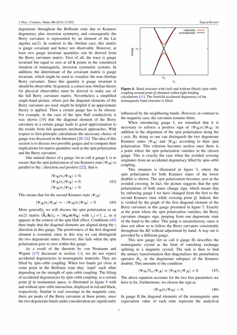
Figure 9. Left: the crossing of some p bands of a ferromagnetic simple cubic band structure near the center of the Brillouin zone. Right:conical intersection of energy surfaces near point P. The z axis represents the energy dispersion of two intersecting bands over an arbitraryplane in k space through the diabolical point. The color scale denotes the spin polarization corresponding to each band.

Figure 10. Left: absolute value of the Berry curvature |Ω| plotted over a plane in k space through the degeneracy point P. Right: inversesquare root of the absolute value, i.e. 1/

√|Ω|.

symmetry possibly reduces the codimension only in thisregion. Level crossings on a high-symmetry line in theBrillouin zone do not necessarily occur on account ofsymmetry as long as the bands are not degenerate at pointsnearby which have the same symmetry.

As an example, in figure 9 a few bands of the bandstructure near the 0 point along a high-symmetry lineare plotted. There occur three crossings between differentbands. On the right-hand side, the energy dispersion in aplane through the degeneracy marked by P is displayedin order to show the cone shape of the intersection. Thecolor scale represents the spin polarization 〈9|σz|9〉 of thecorresponding band. Within one band the spin polarizationrapidly changes in the vicinity of the degeneracy. At thedegeneracy itself it jumps due to the cusp of the correspondingband. However, when passing the intersection along a straightline in k space and jumping from the lower to the upper bandapparently the spin polarization does not change at all. Thisis a clear indication that the character of the two bands isexchanged at the intersection.

The behavior of the spin polarization near the diabolicalpoint illustrates how observables are influenced by otherbands nearby. The Berry curvature can be viewed as a measureof this coupling, which becomes evident from equations (71)and (72), where a sum over all other bands is performedweighted by the inverse energy difference. Hence, the Berrycurvature of a single Bloch band generally arises due tothe restriction to this band and it becomes large when other

bands are close. As we have seen before, a degeneracyproduces a singularity of the Berry curvature and the adiabaticsingle-band approximation fails.

In our case, the origin of the Berry curvature is thespin–orbit coupling. Since degenerate or almost degeneratepoints in the band structure produce large spin mixing of theinvolved bands, a peak in the Berry curvature can also beunderstood from this point of view.

As discussed in section 1.4, we would expect thecurvature around the degeneracy to obey the 1/|k − k∗|2 lawof a Coulomb field. The asymptotic behavior becomes evidentwhen plotting 1/

√|Ω| in a plane in which the degeneracy is

located (see figure 10 with k∗ = (0, 0, kP)). We observe anabsolute value function |k− k∗|, which proves that the Berrycurvature really has the form of the monopole field strengthgiven by equation (40).

Besides the absolute value we can also examine thedirection of the Berry curvature vector. In figure 11, werecognize the characteristic monopole field. In the lower bandthe monopole is a source, in the upper band a drain, of theBerry curvature. This has been expected because a monopolein one band has to be matched by a monopole of oppositecharge in the other band involved in the degeneracy.

In general, we may assign a ‘charge’ g to the monopoleas in equation (42). This charge is quantized to be eitherinteger or half integer. In order to determine the chargenumerically one could perform a fit of the numerical data withthe monopole field strength. However, there is no reason to

12


Figure 11. Normalized Berry curvature vector around P (compare figure 9, right panel).

Figure 12. The value of the integral equation (75) over a sphericalsurface for the upper band is plotted against the radius of the sphere.

believe that all directions in k space must be equivalent. Somedistortion in a certain direction might result in ellipsoidalisosurfaces of |Ω| instead of spherical ones. A differentapproach, independent from the coordinate system, exploitsequation (41)∫

Vd3k∇k ·Ωn(k) =

∫∂V

ds n ·Ωn(k) = 2πm m ∈ Z,

(75)

where the vector n is normal on the bounding surface ∂V ofsome arbitrary volume V . Performing the numerical surfaceintegration causes no problem since the Berry curvature isanalytical on the surface, unlike the case at the degeneracy. Soas to validate this formula, the Berry curvature flux througha sphere of radius |k − k0| centered at a generic point k0 inthe Brillouin zone near P (see figure 9) is evaluated. This fluxdivided by 2π as a function of the sphere’s radius is plotted infigure 12.

The integral is observed to be quantized to integermultiples of 2π . When increasing the radius of the spherethe surface crosses various diabolical points. Each time thishappens the flux jumps by ±2π depending on whetherthe charge of the Berry curvature monopole is positive ornegative. According to equation (75), this confirms thatthe charges of the monopoles created by the point-likedegeneracies are g = ±1/2. Altogether there are six jumps,

which means there are six diabolical points in the vicinity ofthe point P (see figure 9). Two of the monopoles in the upperband have a negative, the other four a positive, charge of 1/2.A generic point such as the center of the integration sphere ischosen to avoid crossing more than one diabolical point at atime. The deviations from a perfect step function are due to thediscretization of the integral, which increases the error whenthe surface crosses a monopole. The step functions also verifythe statement that monopoles are the only possible sources ofthe Berry curvature.

Haldane [16] describes the dynamics of these degenera-cies with respect to the variation of some control parameter,including the creation of a pair of diabolical points andtheir recombination after relative displacement of a reciprocallattice vector. In the considered case an obvious choice for thecontrol parameters would be λ or Vxc, regulating the strengthof spin–orbit coupling or exchange splitting, respectively.

Thus, the tight-binding code provides an excellent tool foran investigation of the effects connected with the accidentaldegeneracy of bands (see for instance, [16]) since one mayscan through a whole range of parameters without consumingmany computational resources and still obtain qualitativelyreliable results.

2.3. Wannier interpolation scheme

The first method developed specifically for calculating theBerry curvature of Bloch electrons using the full machineryof the density functional theory (DFT) was based on theWannier interpolation code of Marzari et al [29]. As in thecase of the KKR method presented in section 2.1, the essenceof this approach by Wang et al [21] is that it avoids takingthe derivative of the periodic part of the Bloch functionun(r,k) with respect to k numerically by finite differences.A second almost equally important feature is that it offersvarious opportunities to interpolate between different k pointsin the Brillouin zone and hence reduces the number of pointsat which full ab initio calculations need to be performed.

Note that the formulas, naturally arising in wave packetdynamics, for the Berry connection and curvature, given byequations (20) and (21), involve the real space integrals over aunit cell only. Extending them to cover all space by using the

13


Wannier functions defined as

|Rn〉 =Vuc

(2π)3

∫BZ

d3k e−ik·R|9nk〉 , (76)

the Bloch theorem and some care with the algebra, one findsthe following remarkably simple results [21, 30]:

An(k) =∑

R

〈0n| r |Rn〉 eik·R and

Ωn(k) = i∑

R

〈0n|R× r |Rn〉 eik·R.(77)

The matrix elements with respect to the Wannier states,as usual, involve integrals over all space. These formulasturn up and play a central role in the method of Wanget al [21] and make the Wannier interpolation approachlook different from that based on the KKR method, whichmakes use of expansions and integration within a singleunit cell only. The lattice sums in equations (77) do nothave convenient convergence properties, as they depend onthe tails of the Wannier functions in real space. Importantto note is the fact that the phase freedom of the Blochstates allows for an optimization of these tails to reducethe numerical effort. By now an efficient procedure giving‘maximally localized’ Wannier functions [29, 30] has beendeveloped to deal with this issue. Interestingly, in thisprocedure matrix elements of both ∇k and r, as in the KKRmethod discussed in section 2.1, occur. Reassuringly, it isfound that in both approaches an easy to evaluate matrixelement of ∇k dominates over what is frequently calledthe dipole contribution involving matrix elements of r. TheWannier orbitals are localized but, unlike the orbitals inthe tight-binding method, exact representations of the bandstructure of a periodic solid within this method are possibleonly for a limited energy range. For metals, its use in modernfirst-principle calculations is based on the unique ‘maximallylocalized orbitals’ and its power and achievements are wellsummarized in [29]. Here we wish to recall only the bareoutline of the new development occasioned by the currentinterest in the geometrical and topological features of theelectronic structure of crystals.

The method based on the Wannier interpolation scheme,fully described in [21], starts with a conventional DFTcalculation of Bloch states |9nq〉 in a certain energy rangeand on a selected mesh of q points based on a plane-waveexpansion. Then the matrix elements of various operators maybe constructed with respect to a set of maximally localizedWannier states |Rn〉. It should be mentioned that generallythese states are distinct from the Wannier states defined inequation (76) since they are solutions of a procedure tominimize the real space spread of the Wannier functions [30].The minimization is always possible due to the freedomchoosing an arbitrary phase in the definition of Bloch statesas mentioned above. In general, this freedom in defining theBloch states can be written in terms of a unitary operator. Ifwe assume a set of Wannier states chosen according to thisprocedure, the phase sum of these states

〈r|uWn (k)〉 =

∑R

e−ik·(r−R)〈r|Rn〉 (78)

can be defined for an arbitrary k point, which may be at orin between the first-principle q-point mesh. It can be regardedas a ‘Wannier gauge’ representation of the periodic part ofa Bloch state but they are generally no eigenstates of thek-dependent Hamiltonian. In the following one has to evaluatethe matrix elements with respect to the constructed states

HWnm(k) =

∑R

e+ik·R〈0n| H |Rm〉 ,

∇HWnm(k) =

∑R

e+ik·RiR 〈0n| H |Rm〉 ,

AWnm(k) =

∑R

e+ik·R〈0n| r |Rm〉 ,

ΩWnm(k) = i

∑R

e+ik·R〈0n|R× r |Rm〉 .

(79)

Actually, all of them are given in the same ‘Wannier gauge’.The indices n and m refer to the full bundle of Wannier statesselected to represent the real bands up to a certain energyabove the Fermi level.

The next step is to find unitary matrices ¯U(k) such that

¯U†(k) ¯H

W(k) ¯U(k) = ¯H

H(k) with

HHnm(k) = Enkδnm, (80)

where the eigenvalues Enk should agree with the first-principledispersion relation of the bands chosen to be represented. Thecorresponding eigenfunctions

|uHn (k)〉 =

∑m

Unm(k)|uWm (k)〉 (81)

should reproduce the periodic part of these states.Thus, |uH

n (k)〉 can be used to evaluate equations (20)and (21) for the Berry connection and the curvature in thestandard way. However, such direct calculations are preciselynot what one would like to do. The point of Wang et al is thatthe above preamble offers an alternative. Namely, the unitarytransformation ¯U(k) transforms all states and operators fromthe ‘Wannier gauge’ to another gauge which is called the‘Hamiltonian (H) gauge’ and one can transform all the easy toevaluate ‘Wannier gauge’ operators in equation (79) into their‘Hamiltonian gauge’ form. Of course, ΩH

nm(k) is of particularinterest. Unfortunately, due to the k dependence of Unm(k) theform of equations (20) and (21) is not covariant under such atransformation. For instance, the connection is given by

AH= U†AWU + iU†

∇U = AH+ iU†

∇U, (82)

where for clarity the momentum dependency has beendropped as we will mainly do within this section. All productsare matrix multiplications and the gradient is taken withrespect to k. A similar, but more complicated formula can

be derived for ΩH. The matrices AH,Ω

H, and H

Hdenote

the covariant components, that is to say the part of thetransformed operator which does not contain U†∇U, of AH

and HH, respectively. If we write ΩH= U†ΩWU and

DHnm = (U

†∇U)nm =

(U†∇HWU)nm

Em − En(1− δnm), (83)

14


Figure 13. Left: Berry curvature z(k) of Fe along symmetry lines with a decomposition into three different contributions of equation (84)(note the logarithmic scale). Right: Fermi surface in the (010) plane (solid lines) and the total Berry curvature −z(k) in atomic units (colormap). Reproduced with permission from [21]. Copyright 2006 American Physical Society.

the final formula for the total Berry curvature Ω(k) =∑nfnΩn(k), including the sum over all occupied states, reads

as follows:

Ω(k) =∑

nfnΩ

Hnn +

∑n,m

(fm − fn)DHnm × A

Hmn +ΩDD, (84)

where the last term takes the form

ΩDD= i/2

∑n,m(fn − fm)

(U†∇HWU)nm × (U†∇HWU)mn

(Em − En)2.

(85)

Here fn ≡ fn(k) and fm ≡ fm(k) are the equilibriumdistribution functions for bands n and m, respectively. Thesums in equation (84) run over all Wannier states used for anaccurate description of the occupied states. Interestingly, thisis the standard form of the Berry curvature for a Hamiltonianwhich depends parametrically on k and it also shows up asone of the contributions in the KKR and the tight-bindingapproaches discussed in sections 2.1 and 2.2. Reassuringly,computations by all three methods find the contributionfrom such terms as equation (85) dominant and almostexclusively responsible for the spiky features as functions ofk. As noted in the introduction, these features originate fromband crossings or avoided crossings and have a variety ofinteresting physical consequences.

For instance, the Berry curvature calculated by Wanget al [21, 31], shown in figure 13, leads directly to agood quantitative account of the intrinsic contribution to theanomalous Hall effect in Fe. The left panel of figure 13shows the decomposition of the Berry curvature in differentcontributions arising from the expansion of the states intoa Wannier basis (see equation (84)). Noting the logarithmicscale, it is evident that the dominant contribution stems fromthe Berry curvature ΩDD(k) of the k-dependent HamiltonianH

H(k) according to equation (85). The other terms including

matrix elements of the position operator r are negligible,which is similar to what turned out to be the case within theKKR method. Further applications of the considered methodto the cases of fcc Ni and hcp Co [31, 32] are equallyimpressive.

2.4. Kubo formula

2.4.1. Anomalous Hall conductivity and the Berry curvature.Most conventional approaches to the electronic transport insolids are based on the very general linear response theoryof Kubo [33]. Indeed, the first insight into the cause ofthe anomalous Hall effect by Karplus and Luttinger [34]was gained by deploying the Kubo formula for a simplemodel Hamiltonian of electrons with spin. In this sectionwe review briefly the first-principle implementation of theKubo formula in aid of calculating the Berry curvature. Thesimple observation which makes this possible is that boththe semiclassical description and the Kubo formula approachyield the same expression for the intrinsic contribution to theanomalous Hall conductivity (AHC). Hence, by comparingthe two, a Kubo-like expression for the Berry curvature canbe extracted. Here we examine the formal connection betweenthe two formulas for the Berry curvature and demonstratethat they are equivalent, as was mentioned already by Wanget al [21].

The Kubo formula for the AHC in the static limit fordisorder-free noninteracting electrons is given by [35]

σxy = e2h∫

BZ

d3k

(2π)3∑

n

∑m6=n

fn(k)

×Im[〈9nk|v|9mk〉 × 〈9mk|v|9nk〉]z

(Enk − Emk)2, (86)

whereas in the semiclassical approach it is expressed in termsof the Berry curvature [7, 14, 34, 41]

σxy = −e2

h

∑n

∫BZ

d3k

(2π)3fn(k)z

n(k). (87)

Assuming the equivalence of the two approaches, acomparison of equations (86) and (87) yields a Kubo-likeformula for the Berry curvature. However, the equivalence isnot a priori evident and has to be proven, which will be donein the following.

The starting point is the Berry curvature written in termsof the periodic part of the Bloch function

Ωn(k) = i 〈∇kun(k)| × |∇kun(k)〉 . (88)

15


Let us follow the route given by Berry [3] to rewrite thisexpression. Introducing the completeness relation with respectto the N present bands, 1 =

∑Nm=1|um〉〈um|, excluding the

vanishing term with m = n and using the relation

〈∇un(k)|um(k)〉 =〈un(k)|∇kH(k) |um(k)〉

Enk − Emk, (89)

which follows from 〈un(k)|H(k)|um(k)〉 = Emk〈un(k)|um(k)〉= 0, yields

Ωn(k) =

i∑m6=n

〈un(k)|∇kH(k) |um(k)〉 × 〈um(k)|∇kH(k)|un(k)〉(Enk − Emk)2

.

(90)

If we reformulate it with respect to the Bloch functions

Ωn(k) = i∑m6=n

〈9nk|eikr∇kH(k)e−ikr

|9mk〉

× 〈9mk|eikr∇kH(k)e−ikr

|9nk〉

× (Enk − Emk)2−1

(91)

and use the relations

H(k) = e−ikrHeikr, (92)

∇kH(k) = ie−ikr[Hr− rH

]eikr= h e−ikrveikr, (93)

we end up with a Kubo-like formula widely used in theliterature [37, 38]

Ωn(k) = ih2∑m6=n

〈9nk|v|9mk〉 × 〈9mk|v|9nk〉

(Enk − Emk)2 . (94)

This formula proves the equivalence of the two approachesfor calculating the AHC as given by equations (86) and(87). In principle, all occupied and unoccupied states have tobe accounted for in the sum of equation (94). However, inpractice only states with energies close to Enk play a role. Animportant feature of this form is that it is expressed in termsof the off-diagonal matrix elements of the velocity operatorwith respect to the Bloch states. To deal with them a techniquewas adopted, which served well for computing the opticalconductivities [39, 40], where the same matrix elements havebeen required.

The first ab initio calculation of the Berry curvature wasactually performed for SrRuO3 by Fang et al [36] usingequation (94). The authors nicely illustrate the existence ofa magnetic monopole in the crystal momentum space, whichis shown in figure 14. The origin of this sharp structureis the near degeneracy of bands. It acts as a magneticmonopole. A similar effect was found for Fe by Yao et al [41].They demonstrate that for k points near the spin–orbitdriven avoided crossings of the bands the Berry curvatureis extremely enhanced as shown in figure 15. In addition,the agreement between the right panels of figures 13 and 15shows impressively the equivalence between the two differentmethods.

Figure 14. Calculated Berry curvature (in [36] called flux bz)z(k) =

∑n∈t2g

zn(k) distribution in k space for t2g bands as a

function of (kx, ky) with kz = 0 for SrRuO3 with cubic structure.Reproduced with permission from [36]. Copyright 2003 AAAS.

2.4.2. Spin Hall conductivity and the Berry curvature. Ofcourse, the fact that the results of the semiclassical transporttheory and the quantum mechanical Kubo formula agreeexactly, as was shown above, is surprising. In general, itcannot be expected for all transport coefficients. Indeed, aswe shall now demonstrate, the situation is quite different forthe spin Hall conductivity.

Evidently, the Kubo approach is readily adopted tocalculate the spin-current response to an external electric fieldE. Although there is still a controversy about an expressionfor the spin-current operator to be taken [42–45], frequentlythe following tensor product of the relativistic spin operatorβΣ and the velocity operator v is used:

JSpin= βΣ⊗ v, βΣ =

(σ 0

0 −σ

). (95)

Furthermore, the symmetrized version of the tensor productis often used in literature and the spin-current response iscalculated as the expectation value of the operator JSpin.However, within the Dirac approach we have

v = cα = c

(0 σ

σ 0

)and

β6ivj − vjβ6i = 0, if i 6= j.

(96)

Similar to the formula for the charge Hall conductivity, onefinds for the spin Hall conductivity with spin polarization inthe z direction [43, 37, 38]

σ zxy =

e2

h

∑k,n

σ zxy;n(k)fn(k), (97)

where the k and band resolved conductivity σ zxy;n(k) in the

framework of the Kubo formula (Kubo) is given by

σ zxy;n(k)Kubo =

− h2∑m6=n

Im[〈9nk|β6zvx|9mk〉〈9mk|vy|9nk〉]

(Enk − Emk)2. (98)

16


Figure 15. Left: band structure of bulk Fe near Fermi energy (upper panel) and Berry curvature z(k) (lower panel) along symmetry lines.Right: Fermi surface in (010) plane (solid lines) and Berry curvature −z(k) in atomic units (color map). Reproduced with permissionfrom [41]. Copyright 2004 American Physical Society.

In the literature, this quantity is sometimes even called spinBerry curvature [38], analogously to the AHE. This notationis misleading and should not be used.

Let us tackle the same problem from the point of view ofthe semiclassical theory (sc). This suggests that one shouldtake the velocity in equations (95) to be the anomalousvelocity given by equation (11). This argument leads to [5,42]

σ zxy;n(k)sc = Tr[ ¯S

z

n(k)¯

zn(k)]. (99)

Here ( ¯Sz

n(k))ij = 〈9nik|β6z|9njk〉 is the spin matrix for a

Kramers pair labeled by i, j and ¯zn(k) is the non-Abelian

Berry curvature [19] introduced in section 1.3. The pointwe wish to make here is that this formula is not equivalentto the Kubo form in equation (98). The reason is thatthe band off-diagonal terms of the spin matrix wereneglected in the derivation from the wave packet dynamicsof equation (99) [5].

Evidently, σ zxy;n(k)Kubo cannot be written as a single-band

expression, in contrast to the case of the AHC, which turnedout to be exactly the conventional Berry curvature (seesection 2.4.1). The contributions of equation (98) which wereneglected in equation (99) are of quantum mechanical originand are not accounted for in the semiclassical derivation.Culcer et al [42] tackled the problem and identified theneglected contributions, without giving up the wave packetidea, as spin and torque dipole terms. Nevertheless, it wasshown that under certain approximations a semiclassicaldescription may result in quantitatively comparable results tothe Kubo approach [19]. This will be discussed in section 3.

3. Intrinsic contribution to the charge and spinconductivity in metals

Here we discuss applications of the computational methodsfor the Berry curvature discussed in section 2. We will focuson first-principle calculations of the anomalous and spin Hall

conductivities. The anomalous Nernst conductivity, closelyrelated to it, will be also discussed briefly.

The first ab initio studies of the AHE, based onequation (87) with Ωn(k) defined by equation (94), werereported in [36, 46]. As is well known, the conventionalexpression for the Hall resistivity

ρxy = R0Bz + 4πRsMz (100)

(where Bz is the magnetic field in the z direction and R0and Rs are the normal and the anomalous Hall coefficient,respectively) assumes a monotonic behavior of ρxy as wellas σxy as a function of the magnetization M. By meansof first-principle calculations based on the pseudopotentialmethod (STATE code), Fang et al [36] have shown that theunconventional nonmonotonic behavior of the AHC measuredin SrRuO3 (figure 16, left) is induced by the presence of amagnetic monopole (MM) in momentum space (see figure 14and the corresponding discussion in section 2.4.1). Theexistence of MMs causes the sharp and spiky structure of theAHC as a function of the Fermi-level position, shown in theright panel of figure 16. At the self-consistently determinedFermi level, the calculated value σxy = −60 ( cm)−1 iscomparable with the experimentally observed conductivityof about −100 ( cm)−1. Obviously, a small change in theFermi level would cause dramatic changes in the resultingAHC. Indeed, as was shown in [46], the calculated AHCof ferromagnetic Gd2Mo2O7 and Nd2Mo2O7 is stronglychanged by the choice of the Coulomb repulsion U varied inthe used mean-field Hartree–Fock approach.

A year later, results for the intrinsic AHC in ferromag-netic bcc Fe, based on the full-potential linearized augmentedplane-wave method (WIEN2K code), were published [41].The authors used the same Kubo formula approach to describethe transversal transport. In particular, a close agreementbetween theory, σxy = 751 ( cm)−1, and experiment, σxy =

1032 ( cm)−1, was found, that points to the dominance ofthe intrinsic contribution in Fe. A slow convergence of thecalculated value for the AHC with respect to the numberof k points was reported. The reason for the convergence

17


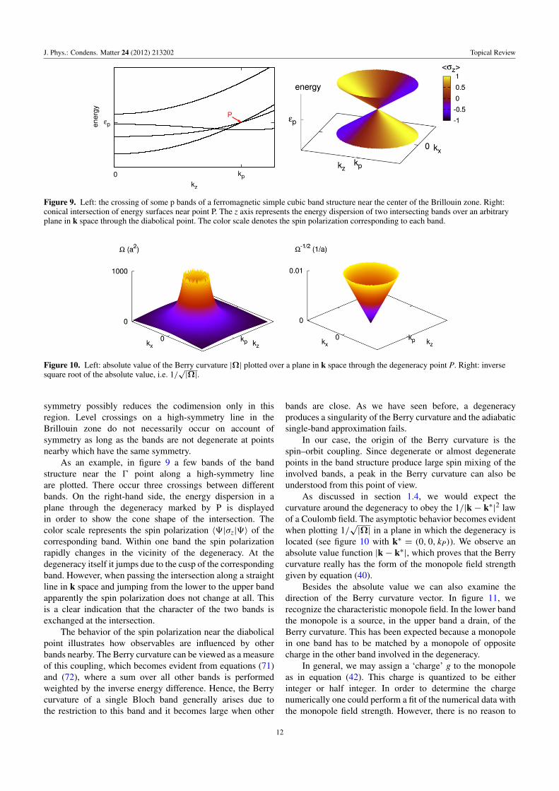
Figure 16. Left: the Hall conductivity σ zxy of SrRuO3 as a function of the magnetization along z. Right: σ z

xy as a function of the Fermi-levelposition for the orthorhombic structure of SrRuO3. Reproduced with permission from [36]. Copyright 2003 AAAS.

Figure 17. Left, (a) relativistic band structure and (b) spin Hall conductivity for variable Fermi level of fcc Pt (reproduced with permissionfrom [47]. Copyright 2008 American Physical Society); right, (a) relativistic band structure and (b) spin Hall conductivity of fcc Au(reproduced with permission from [48]. Copyright 2009 American Institute of Physics). The dashed curves in the left panel represent thescalar-relativistic band structure. The real Fermi level is set as the zero of the energy scale.

problems is given by small regions in momentum spacearound avoided crossings and enhanced spin–orbit coupling.In the behavior of the Berry curvature these points causestrong peaks, which is shown in figure 15. If both relatedstates of the avoided crossing are occupied, their combinedcontribution to the AHC is negligible since they compensateeach other. However, when the Fermi level lies in a spin–orbitinduced gap, the occupied state, which acts now as an isolatedmagnetic monopole, causes a peak in the AHC. Consequently,it was necessary to use millions of k points in the firstBrillouin zone to reach convergence.

To avoid such demanding computational efforts, theWannier interpolation scheme, discussed in section 2.3,was suggested and applied for Fe in [21]. The authorsstarted with the relativistic electronic structure obtained bythe pseudopotential method (PWSCF code) at a relativelycoarse k mesh. Using maximally localized Wannier functions,constructed from the obtained Bloch states, all quantitiesof interest were expressed in the tight-binding like basisand interpolated onto a dense k mesh. Finally, this newmesh was used to calculate the AHC. The obtained value of756 ( cm)−1 is in good agreement with the result of [41].

The same scheme was used further on to calculatethe AHC applying Haldane’s formula [16] which meansintegration not over the entire Fermi sea, as is required by

the Kubo formula, but only over the Fermi surface. Theresults obtained for Fe, Co, and Ni [31] agreed very well forboth procedures and with previous theoretical studies [41].Moreover, the work done by the group of Vanderbilt [21]has stimulated further first-principle calculations as will beshown below. The first ab initio calculations of the spin Hallconductivity (SHC) were performed for semiconductors andmetals [37, 38]. The description of the electronic structurein [38] was based on the full-potential linearized augmentedplane-wave method (WIEN2K code) and in [37] on theall-electron linear muffin-tin orbital method, but both relyon the solution of the Kubo formula given by equation (98)to describe the SHC. Later, in [47] the relatively large SHCmeasured in Pt was explained by the contribution of thespin–orbit split d bands at the high-symmetry points L andX near the Fermi level (figure 17, left). In contrast, Au [48]shows similar contributions to the SHC, but at lower energieswith respect to the Fermi level EF, since the extra electron ofAu with respect to Pt causes full occupation of the d bands(figure 17, right).

The spin–orbit coupling is the origin of the AHE andthe SHE. In particular, the avoided crossings significantlyincrease these effects. In addition, the spin–orbit couplinglinks the spin degree of freedom to the crystal lattice,which is the source of the anisotropy with respect to

18


Figure 18. Spin Hall conductivities σ xyz and σ z

xy for several hcp nonmagnetic metals and for antiferromagnetic Cr. Reproduced withpermission from [49]. Copyright 2010 American Physical Society.

Figure 19. The intrinsic spin Hall conductivity for fcc Pt (left) and Au (right) [19]. The Fermi level is set to zero on the energy scale.Reproduced with permission from [19]. Copyright 2011 American Physical Society.

the chosen quantization axis; this means σ xyz and σ z

xy maydiffer. This was demonstrated first for the AHE in hcpCo [32] and later for the SHE in several nonmagnetic hcpmetals [49] (figure 18). Here, the pseudopotential method(PWSCF code) and the full-potential linearized augmentedplane-wave method (FLEUR code) were used for the AHEand SHE, respectively. To reduce the computational efforts,the Berry curvature calculations were based on the Wannierinterpolation scheme according to [21]. These methods wereapplied to several situations in ordered alloys [50] where theanisotropy of the AHC [51] was discussed as well and theroles of spin-conserving and non-spin-conserving parts of theSOC were discussed in detail [52]. Very recently the samegroup calculated the scattering-independent contribution tothe side jump mechanism for the anomalous Hall effect [53].The used approach is based on a model assuming short-rangeuncorrelated disorder and involves the Berry connection of theBloch states as an essential part [54].

Finally, an approach for calculating the SHC based onthe KKR method was proposed ([19], section 2.1). Forthe description of the transversal spin transport the authorsapplied an approach different from the widely used Kuboformula. Their calculations are based on the expression forthe SHC in the non-Abelian case suggested in [5]. Thisexpression was simplified further by the approximation thatthe expectation value of the β6z operator is assumed tobe +1 and −1 for the two spin degenerate states, arising

in nonmagnetic crystals with inversion symmetry. Thus, thesemiclassical treatment was reduced to the two current modelwith the final expression for the SHC in terms of the usualformula for the AHC at zero temperature

σ zxy =

e2

h(2π)3

∫ EF

dE z(E), (101)

where z(E) is defined by equation (65). The spin Hallconductivities σ z

xy(E) considered for a variable Fermi level,and calculated for Pt and Au in such an approach (figure 19),are quantitatively in good agreement with the ones obtainedby the Kubo-like formula (see figure 17).

Related to the already discussed calculation of theintrinsic spin and anomalous Hall conductivities is theintrinsic mechanism of the anomalous Nernst effect. It isdriven by an applied thermal gradient instead of the appliedelectric field. The two driving forces are of physicallydifferent nature. The electric field is a mechanical force incontrast to the statistical force of a temperature gradient.Nevertheless, as was shown by Xiao et al [55], the finalexpression for the anomalous Nernst conductivity αxy at lowtemperatures is simply given by the Mott relation

αxy =π2

3

k2BT

eσ ′xy(EF). (102)

Here σ ′xy(EF) is the first energy derivative at EF of theintrinsic anomalous Hall conductivity, defined in terms of

19


Figure 20. The intrinsic anomalous Nernst conductivity (dividedby the temperature T) of the CuCr2Se4−xBrx alloy as a function ofthe Br content x. Reproduced with permission from [55]. Copyright2006 American Physical Society.

the Berry curvature in equation (87). All the above methodsto calculate the Berry curvature can be applied to computethe anomalous Nernst conductivity as well. In figure 20 acomparison between experimental results and first-principlecalculations for the alloy CuCr2Se4−xBrx are shown. Theconcentration dependence is described by using a rigid bandmodel. The agreement is relatively good despite the factthat the experiment cannot resolve the peak–valley structurearound x = 0.2.

4. De Haas–van Alphen oscillation and the Berryphases

Other phenomena related to the topic of this review arevarious quantum oscillations. For their proper descriptiontypically the Berry phase accumulated along a closed orbit inparameter space is needed, which can be expressed via theBerry curvature of the system. For instance, in the case ofthe de Haas–van Alphen effect, the semiclassical formula forthe quantized energies of the Landau levels includes a terminvolving the Berry phase of the corresponding orbits in kspace. This was pointed out by Mikitik and Sharlai [56, 57],who have discussed a number of interesting experiments inthese terms [58, 59]. They argue that the quasiparticles whichmove along closed orbits in response to an external magneticfield B are wave packets, in the sense of the semiclassicaltheory, and therefore their semiclassical equations (8) and(9) are subject to corrections arising from Berry phasesand curvatures. In short, a closed orbit is defined by therequirement that the energy of the wave packet Enk −M(k)Bis equal to E = constant for all k along the orbit. Here M(k)is the spin plus the orbital magnetic moment of the electronalong the path. Then the Bohr–Sommerfeld quantizationcondition for E = Eν to be a Landau level is [1, 57, 60]

S(Eν, kz) = 2π heBz

(ν +

12−γn

2π

), (103)

where S(Eν, kz) is the area enclosed by the orbit in k space.The Berry phase accumulated along the orbit labeled by C is

given by

γn =

∮C

dk ·An(k) =∫∫

Sc

dS ·Ωn(k), (104)

where Sc is any surface in k space whose boundary is C.Clearly, the presence of the orbital magnetization in the theoryindicates that the change of the band energy due to spin andorbital motion is taken into account. This important fact ismore evident if equation (103) is recast as

S0(Enk, kz) = 2π heBz

×

(ν +

12−γn

2π−

12π

∮C0

Mz(k) dk|∂Enk/∂k⊥|

),

(105)

where S0(Enk, kz) is the area enclosed by an orbit C0 on aniso-energetic surface of the actual band structure. From thepoint of view of analyzing the high quality data availablefrom de Haas–van Alphen measurements, the physical contentof the above formula is of considerable general interest,and shows the necessary correction of the common theory.However, to calculate the loop integral in equation (105) forthe general case with spin–orbit coupling is a real challenge,which has been, so far, only partially implemented6.

The full theory has already been presented by Roth in1966 [61], although never applied to analyze experimentaldata. Only recently the formulas have been revisited in viewof the new light cast on them by advances in describing wavepackets driven by external fields and the associated Berryphases.

To highlight the significance of the Berry phase andcurvature in the present context, we shall now consider thesimple case where the spin, and therefore the spin–orbitcoupling, is altogether neglected and it is assumed that thesystem is time-reversal and inversion symmetric. In this caseone might think that the Berry phase would vanish since theBerry curvature is zero over the full Brillouin zone. However,as was shown by Mikitik and Sharlai [56, 57], this is not trueif the semiclassical orbit encloses a line of degeneracy. As wasshown in [58, 59] for several materials, such lines exist in theabsence of spin–orbit coupling and have a significant effect onthe observable de Haas–van Alphen frequencies.

Here we focus on two hexagonal systems, Mg and Tl, anddiscuss the results for γn, given by equation (104), obtainedwith the KKR method [22, 19]. In figure 21 the band structureof Mg along the 0M direction clearly shows an accidentaldegeneracy, which is actually part of a full line in the kz = 0plane as shown in the right panel of figure 21. Furthermore,this line is enclosed by one sheet of the Fermi surface, whichallows us to study the effect. If the magnetic field is applied indifferent directions as shown in figure 22, orbits either enclosethe line of degeneracy, as in the case shown in red, or they donot, shown in black. We have evaluated the integrals over aselection of those loops numerically and found γn = π forall orbits which enclose the line and γn = 0 for all thosewhich do not. The important fact is that the integral value

6 See for example [63] and citations [9–30] in [62].

20


Figure 21. Left panel: band structure of hcp Mg along the 0M direction. The accidental degeneracy of two bands is part of a line ofdegeneracy in the kz = 0 plane. The inset shows the lifting of the degeneracy due to spin–orbit coupling. Right panel: the full line ofdegeneracy which is enclosed by the Fermi surface of the second band.

Figure 22. Fermi surfaces for Cu (a) and Mg (b) with extremal orbits for different directions of the applied magnetic field. For Tl (c) aconstant energy surface slightly above the Fermi energy (EF + 0.02 Ryd) was chosen to create extremal orbits enclosing a line of contactpoints. These orbits on tiny ellipsoids in the 0M direction are shown in red and black for B fields parallel and perpendicular to the hcp baseplane respectively. The lines of degeneracy are shown as blue dashed lines.

is independent of the actual form of the loop. The effect istopological since only whether the line penetrates the orbit ornot is relevant. This result dramatically affects the analysisof de Haas–van Alphen experiments since the quantizationcondition of equation (103) will be either

S(Eν, kz) = 2π heBzν (106)

or

S(Eν, kz) = 2π heBz(ν +12 ) (107)

depending on whether the orbit encloses a line of degeneraciesor not, respectively.

Clearly, what happens to such lines of degeneracies inthe presence of spin and spin–orbit coupling is an interestingand fundamental question, since in that case the bandsare formed from states that are Kramers doublets and twosuch doublets are infinitely unlikely to be degenerate. Inthe limit of small spin–orbit coupling this question wasinvestigated by Mikitik and Sharlai [62]. They found that theBerry phase contribution becomes zero, but for nonmagneticinversion symmetric systems there is a contribution to the areaenclosed by a Landau orbit arising from the magnetization

part of equation (105). However, the case of strong spin–orbitcoupling remains an open problem.

5. Conclusion

In the presence of a periodic crystal potential the free electron

spectrum Ek =h2k2

2m breaks up into bands with nontrivialdispersion relations Enk. It turns out that the adiabaticdynamics of wave packets, constructed by superpositionof all k states but a limited number of bands n, featuresa Berry connection An(k) and a corresponding curvatureΩn(k), which account for the influence of the neglectedbands [6, 7]. Moreover, these geometrical properties of theband structure play an essential role in describing a numberof important physical phenomena such as spin and chargetransport, electric polarization and orbital magnetization [1].What makes these remarkable developments particularlyinteresting from the point of view of first-principle electronicstructure calculations is the fact that the curvature Ωn(k) is avery rapidly varying function of k and it depends on intricatedetails of the band structure. Consequently, devising methodsfor computing Ωn(k) have recently become a very active

21


field of research. In this paper we sketched three approachesto the problem: one is based on multiple scattering theory(KKR, similarly LMTO), another one on the Wannier functionrepresentation of first-principle bands and the third one ondirect evaluation of a Kubo-like formula. We pointed outthe differences and highlighted the similarities in the waythe derivatives with respect to the wave vector k enter theproblem. We stressed the importance of level crossings whichgive rise to curvatures Ωn(k) whose k dependence is that ofthe Dirac monopole and the more exotic avoided crossings ofKramers degenerate bands whose curvature is a non-Abeliangauge field. As illustrations of results by the various methods,we presented calculations of the intrinsic contribution to theanomalous and spin Hall conductivity and the Berry curvaturefor a variety of systems as well as the manifestation of theBerry phase in de Haas–van Alphen oscillations.

In that review we concentrated on the Berry curvaturecaused by the parameter k in the Hamiltonian for Blochelectrons. However, from the general point of view any slowlychanging parameter in a Hamiltonian causes curvatures whichmight be of interest in future considerations. From thatperspective, curvatures associated with spatial or temporalparameters will represent new computational challenges.

Very recently, after finalizing this manuscript, anothermethod calculating the Berry curvature was published [64]. Itis based on a finite-differences approach within the augmentedspherical wave scheme. The method was originally developedfor calculating directly the Z2 invariants of topologicalinsulators and not for expressing the Berry curvature k-pointby k-point [65, 66]. This is the reason why we missed it. Wewould like to thank Professor Jurgen Kubler for discussingthis new method with us.

Acknowledgments

One of us (BLG) would like to thank Professor Michael Berryfor many fruitful conversations on the topic of this article. MGacknowledges support from the German Research Foundation(DFG) via a Research Fellowship (GR 3838/1-1). In addition,this work was supported by the DFG via SFB 762.

References

[1] Xiao D, Chang M-C and Niu Q 2010 Berry phase effects onelectronic properties Rev. Mod. Phys. 82 1959

[2] Marder M P 2000 Condensed Matter Physics (New York:Wiley)

[3] Berry M V 1984 Quantal phase factors accompanyingadiabatic changes Proc. R. Soc. A 392 45

[4] Culcer D, Yao Y and Niu Q 2005 Coherent wave-packetevolution in coupled bands Phys. Rev. B 72 085110

[5] Shindou R and Imura K-I 2005 Noncommutative geometryand non-Abelian Berry phase in the wave-packet dynamicsof Bloch electrons Nucl. Phys. B 720 399–435

[6] Wilczek F and Zee A 1984 Appearance of gauge structure insimple dynamical systems Phys. Rev. Lett. 52 2111

[7] Sundaram G and Niu Q 1999 Wave-packet dynamics in slowlyperturbed crystals: gradient corrections and Berry-phaseeffects Phys. Rev. B 59 14915

[8] Kramers H A 1930 General theory of paramagnetic rotation incrystals Proc. R. Acad. Sci. Amsterdam 33 959

[9] Elliott R J 1954 Theory of the effect of spin–orbit coupling onmagnetic resonance in some semiconductors Phys. Rev.96 266

[10] Berry M V and Wilkinson M 1984 Diabolical points in thespectra of triangles Proc. R. Soc. A 392 15

[11] Pientka F 2010 Geometrical concepts in the band theory ofsolids Diploma Thesis University Halle-Wittenberg http://www.physik.uni-halle.de/theorie/ag/qtfk/mitarbeiter/pientka/

[12] Hals K M D, Nguyen A K, Waintal X and Brataas A 2010Effective magnetic monopoles and universal conductancefluctuations Phys. Rev. Lett. 105 207204

[13] Dirac P A M 1948 The theory of magnetic poles Phys. Rev.74 817

[14] Thouless D J, Kohmoto M, Nightingale M P andden Nijs M 1982 Quantized Hall conductance in atwo-dimensional periodic potential Phys. Rev. Lett. 49 405

[15] Simon B 1983 Holonomy, the quantum adiabatic theorem, andBerry’s phase Phys. Rev. Lett. 51 2167

[16] Haldane F D M 2004 Berry curvature on the Fermi surface:anomalous Hall effect as a topological Fermi-liquidproperty Phys. Rev. Lett. 93 206602

[17] von Neumann J and Wigner E 1929 Uber das verhalten voneigenwerten bei adiabatischen prozessen Phys. Z. 30 467

[18] Bohm A, Mostafazadeh A, Koizumi H, Niu Q andZwanziger J 2003 The Geometric Phase in QuantumSystems (Berlin: Springer)

[19] Gradhand M, Fedorov D V, Pientka F, Zahn P, Mertig I andGyorffy B L 2011 On calculating the Berry curvature ofBloch electrons using the KKR method Phys. Rev. B84 075113

[20] Fabian J and Das Sarma S 1998 Spin relaxation of conductionelectrons in polyvalent metals: theory and a realisticcalculation Phys. Rev. Lett. 81 5624

[21] Wang X, Yates J R, Souza I and Vanderbilt D 2006 Ab initiocalculation of the anomalous Hall conductivity by Wannierinterpolation Phys. Rev. B 74 195118

[22] Gradhand M, Czerner M, Fedorov D V, Zahn P,Yavorsky B Yu, Szunyogh L and Mertig I 2009 Spinpolarization on Fermi surfaces of metals by the KKRmethod Phys. Rev. B 80 224413

[23] Pientka F, Gradhand M, Fedorov D V, Mertig I andGyorffy B L 2012 Gauge freedom for degenerate Blochstates Phys. Rev. B submitted

[24] Zeller R, Dederichs P H, Ujfalussy B, Szunyogh L andWeinberger P 1995 Theory and convergence properties ofthe screened Korringa–Kohn–Rostoker method Phys. Rev.B 52 8807

[25] Szunyogh L, Ujfalussy B, Weinberger P and Kollar J 1994Self-consistent localized KKR scheme for surfaces andinterfaces Phys. Rev. B 49 2721

[26] Strange P 1998 Relativistic Quantum Mechanics withApplications in Condensed Matter and Atomic Physics(Cambridge: Cambridge University Press)

[27] Slater J C and Koster G F 1954 Simplified LCAO method forthe periodic potential problem Phys. Rev. 94 1498

[28] Jones M D and Albers R C 2009 Spin–orbit coupling in anf-electron tight-binding model: electronic properties of Th,U, and Pu Phys. Rev. B 79 045107

[29] Marzari N, Souza I and Vanderbilt D 2003 An introduction tomaximally-localized wannier functions Psi-k Newsletter57 129 (Scientific Highlight of the Month) http://www.psi-k.org/newsletters/News 57/Highlight 57.pdf

[30] Marzari N and Vanderbilt D 1997 Maximally localizedgeneralized Wannier functions for composite energy bandsPhys. Rev. B 56 12847

[31] Wang X, Vanderbilt D, Yates J R and Souza I 2007Fermi-surface calculation of the anomalous Hallconductivity Phys. Rev. B 76 195109

22

http://dx.doi.org/10.1103/RevModPhys.82.1959

http://dx.doi.org/10.1103/RevModPhys.82.1959

http://dx.doi.org/10.1098/rspa.1984.0023


http://dx.doi.org/10.1103/PhysRevB.72.085110


http://dx.doi.org/10.1016/j.nuclphysb.2005.05.019

http://dx.doi.org/10.1016/j.nuclphysb.2005.05.019

http://dx.doi.org/10.1103/PhysRevLett.52.2111




http://dx.doi.org/10.1103/PhysRev.96.266




http://www.physik.uni-halle.de/theorie/ag/qtfk/mitarbeiter/pientka/





























































































http://www.psi-k.org/newsletters/News_57/Highlight_57.pdf






























































[32] Roman E, Mokrousov Y and Souza I 2009 Orientationdependence of the intrinsic anomalous Hall effect in hcpCobalt Phys. Rev. Lett. 103 097203

[33] Kubo R 1957 Statistical–mechanical theory of irreversibleprocesses J. Phys. Soc. Japan 12 570

[34] Karplus R and Luttinger J M 1954 Hall effect inferromagnetics Phys. Rev. 95 1154

[35] Sinova J, Jungwirth T, Kucera J and MacDonald A H 2003Infrared magneto-optical properties of (III,Mn)Vferromagetic semiconductors Phys. Rev. B 67 235203

[36] Fang Z, Nagaosa N, Takahashi K S, Asamitsu A, Mathieu R,Ogasawara T, Yamada H, Kawasaki M, Tokura Y andTerakura K 2003 The anomalous Hall effect and magneticmonopoles in momentum space Science 302 92

[37] Guo G Y, Yao Y and Niu Q 2005 Ab initio calculation of theintrinsic spin Hall effect in semiconductors Phys. Rev. Lett.94 226601

[38] Yao Y and Fang Z 2005 Sign changes of intrinsic spin Halleffect in semiconductors and simple metals: first-principlescalculations Phys. Rev. Lett. 95 156601

[39] Wang C S and Callaway J 1974 Band structure of nickel:spin–orbit coupling, the Fermi surface, and the opticalconductivity Phys. Rev. B 9 4897

[40] Guo G Y and Ebert H 1995 Band-theoretical investigation ofthe magneto-optical Kerr effect in Fe and Co multilayersPhys. Rev. B 51 12633

[41] Yao Y, Kleinman L, MacDonald A H, Sinova J, Jungwirth T,Wang D, Wang E and Niu Q 2004 First principlescalculation of anomalous hall conductivity in ferromagneticbcc Fe Phys. Rev. Lett. 92 037204

[42] Culcer D, Sinova J, Sinitsyn N A, Jungwirth T,MacDonald A H and Niu Q 2004 Semiclassical spintransport in spin–orbit-coupled bands Phys. Rev. Lett.93 046602

[43] Sinova J, Culcer D, Niu Q, Sinitsyn N A, Jungwirth T andMacDonald A H 2004 Universal intrinsic spin Hall effectPhys. Rev. Lett. 92 126603

[44] Vernes A, Gyorffy B L and Weinberger P 2007 Spin currents,spin-transfer torque, and spin-Hall effects in relativisticquantum mechanics Phys. Rev. B 76 012408

[45] Lowitzer S, Gradhand M, Kodderitzsch D, Fedorov D V,Mertig I and Ebert H 2011 Extrinsic and intrinsiccontributions to the spin Hall effect of alloys Phys. Rev.Lett. 106 056601

[46] Solovyev I V 2003 Effects of crystal structure and on-siteCoulomb interactions on the electronic and magneticstructure of A2Mo2O7 (A = Y, Gd, and Nd) pyrochloresPhys. Rev. B 67 174406

[47] Guo G Y, Murakami S, Chen T-W and Nagaosa N 2008Intrinsic spin Hall effect in platinum: first-principlescalculations Phys. Rev. Lett. 100 096401

[48] Guo G Y 2009 Ab initio calculation of intrinsic spin Hallconductivity of Pd and Au J. Appl. Phys. 105 07C701

[49] Freimuth F, Blugel S and Mokrousov Y 2010 Anisotropic spinHall effect from first principles Phys. Rev. Lett. 105 246602

[50] Seemann K M, Mokrousov Y, Aziz A, Miguel J, Kronast F,Kuch W, Blamire M G, Hindmarch A T, Hickey B J,Souza I and Marrows C H 2010 Spin–orbit strength drivencrossover between intrinsic and extrinsic mechanisms of theanomalous Hall effect in the epitaxial L10-orderedferromagnets FePd and FePt Phys. Rev. Lett. 104 076402

[51] Zhang H, Blugel S and Mokrousov Y 2011 Anisotropicintrinsic anomalous Hall effect in ordered 3dPt alloys Phys.Rev. B 84 024401

[52] Zhang H, Freimuth F, Blugel S and Mokrousov Y 2011 Roleof spin–flip transitions in the anomalous Hall effect of FePtalloy Phys. Rev. Lett. 106 117202

[53] Weischenberg J, Freimuth F, Sinova J, Blugel S andMokrousov Y 2011 Ab initio theory of thescattering-independent anomalous Hall effect Phys. Rev.Lett. 107 106601

[54] Kovalev A A, Sinova J and Tserkovnyak Y 2010 AnomalousHall effect in disordered multiband metals Phys. Rev. Lett.105 036601

[55] Xiao D, Yao Y, Fang Z and Niu Q 2006 Berry-phase effect inanomalous thermoelectric transport Phys. Rev. Lett.97 026603

[56] Mikitik G P and Sharlai Yu V 1998 Semiclassical energylevels of electrons in metals with band degeneracy linesJ. Exp. Theor. Phys. 87 747

[57] Mikitik G P and Sharlai Yu V 1999 Manifestation of Berry’sphase in metal physics Phys. Rev. Lett. 82 2147

[58] Mikitik G P and Sharlai Yu V 2004 Berry phase andde Haas–van Alphen effect in LaRhIn5 Phys. Rev. Lett.93 106403

[59] Mikitik G P and Sharlai Yu V 2007 The phase of theHaas–van Alphen oszillations, the Berry phase, andband-contact lines in metals Low Temp. Phys. 33 439

[60] Gosselin P, Boumrar H and Mohrbach H 2008 Semiclassicalquantization of electrons in magnetic fields: the generalizedPeierls substitution Europhys. Lett. 84 50002

[61] Roth L M 1966 Semiclassical theory of magnetic energy levelsand magnetic susceptibility of Bloch electrons Phys. Rev.145 434

[62] Mikitik G P and Sharlai Yu V 2002 g factor of conductionelectrons in the de Haas–van Alphen effect Phys. Rev. B65 184426

[63] Erikson O, Ohlsen H and Calais J L 1989 Conduction-electronZeeman splitting in the noble metals Phys. Rev. B 40 5961

[64] Kubler J and Felser C 2012 Berry curvature and the anomalousHall effect in Heusler compounds Phys. Rev. B 85 012405

[65] Xiao D, Yao Y, Feng W, Wen J, Zhu W, Chen X,Stocks G M and Zhang Z 2010 Half-Heusler compounds asa new class of three-dimensional topological insulatorsPhys. Rev. Lett. 105 096404

[66] Fukui T and Hatsugai Y 2007 Quantum spin Hall effect inthree dimensional materials: lattice computation of Z2topological invariants and its application to Bi and SbJ. Phys. Soc. Jap. 76 053702

23



http://dx.doi.org/10.1143/JPSJ.12.570






http://dx.doi.org/10.1126/science.1089408

http://dx.doi.org/10.1126/science.1089408























http://dx.doi.org/10.1063/1.3054362

http://dx.doi.org/10.1063/1.3054362















http://dx.doi.org/10.1134/1.558717

http://dx.doi.org/10.1134/1.558717





http://dx.doi.org/10.1063/1.2737555

http://dx.doi.org/10.1063/1.2737555

http://dx.doi.org/10.1209/0295-5075/84/50002

http://dx.doi.org/10.1209/0295-5075/84/50002













First-principle calculations of the Berry curvature of ... · First-principle calculations of the...

Documents

Transcript of First-principle calculations of the Berry curvature of ... · First-principle calculations of the...