1

First-and second-best allocations under economic and environmental uncertainty

by

Konstantinos Angelopoulos+, George Economides# and Apostolis Philippopoulos*

First draft: October 29, 2010. Accepted: April 25, 2012.

Abstract: This paper uses a micro-founded DSGE model to compare second-best optimal environmental policy, and the resulting Ramsey allocation, to first-best allocation. The focus is on the source and size of uncertainty, and how this affects optimal choices and the comparison between second- and first-best. While higher economic volatility is bad for social welfare in all cases studied, the welfare effects of higher environmental volatility depend on its size and the effectiveness of public abatement policy. The Ramsey environmental tax is pro-cyclical when there is an economic shock, while it is counter-cyclical when there is an environmental shock.

Keywords: General equilibrium; uncertainty; environmental policy; second best. JEL classification: C68; D81; H23.

+ University of Glasgow # Athens University of Economics and Business * Athens University of Economics and Business; CESifo, Munich Corresponding author: Apostolis Philippopoulos, Department of Economics, Athens University of Economics and Business, 76 Patission street, Athens 10434, Greece. Tel: +30-210-8203357. Fax: +30-210-8203301. Email: aphil@aueb.gr

Acknowledgements: We thank two anonymous referees and the two guest editors, Thiess Buettner and Christos Kotsogiannis, for many constructive criticisms and suggestions. We thank Nick Hanley, Saqib Jafarey, Ioana Moldovan, Elissaios Papyrakis, Hyun Park and Tassos Xepapadeas for comments and discussions. We also thank seminar participants at the CESifo workshop on the “Fiscal implications of climate change”, held in Venice, July, 2010. Any remaining errors are ours. This research has been co-financed by the European Union (European Social Fund – ESF) and Greek national funds through the Operational Program "Education and Lifelong Learning" of the National Strategic Reference Framework (NSRF) - Research Funding Program THALIS.

2

1. Introduction

In the presence of environmental externalities, the resulting allocation of resources is

not efficient and hence there is justification for government intervention. In the real

world, where only distorting policy instruments are available, the government has to

choose a second-best optimal policy and therefore a second-best allocation. In the

relevant literature, such second-best policy often takes the form of distorting taxes on

polluting generating activities like output.1

The goal of this paper is to study the importance of the source and size of

uncertainty to second-best environmental tax policy and social welfare, and then

compare this to the associated first-best allocation. As far as we know, this is novel.

We focus on uncertainty because it is a big concern in environmental policy. In

particular, in assessing the risks from climate change and the costs of averting it, there

is a variety of uncertainties that contribute to big differences of opinion as to how, and

how much, to limit emissions (on uncertainty and the environment, see e.g. the

Congressional Budget Office paper prepared for the Congress of the US, 2005).2

Our setup is the standard stochastic neoclassical growth model augmented with

the assumptions that pollution occurs as a by-product of output produced and that

environmental quality has a public good character. Within this setup, there is reason

for policy intervention, which here takes the form of taxes on polluting activities and

use of the collected tax revenues to finance public abatement policy. There are two

exogenous stochastic processes that create extrinsic uncertainty about future outcomes

and drive the stochastic dynamics of the model.3 The first is uncertainty about

production technology (standard shocks to total factor productivity, TFP) and the second

arises from uncertainty about the impact of economic activity on the environment.

Loosely speaking, we call the former shock “economic” and the latter “environmental”.4

We study the implications of extrinsic uncertainty for macroeconomic

outcomes, environmental quality and, ultimately, social welfare in both a second-best

and a first-best framework. Social welfare is defined as the conditional expectation of

the discounted sum of household’s lifetime utility. Regarding second-best allocations,

1 For environmental policy instruments, see the survey by Bovenberg and Goulder (2002). For environmental tax rates in growth models, see the survey by Xepapadeas (2004). 2 There is a rich literature on the role of uncertainty in environmental policy that goes back to Weitzman (1974). For a review of this literature, see Bovenberg and Goulder (2002). 3 Higher extrinsic volatility means a mean-preserving higher standard deviation of shocks to these exogenous processes. 4 The recent BP oil leak in the Gulf of Mexico is an example of such environmental shock.

3

and since the decentralized equilibrium solution depends on the value of the tax rate

employed, we study the case in which the chosen path of tax rates maximizes social

welfare. In particular, we solve for Ramsey tax policy. We then compare second-best

optimal tax policy, and the resulting allocation, to the first-best outcome derived by

solving a fictional social planner’s problem. To solve the model and compute the

associated welfare in each case, we follow Schmitt-Grohé and Uribe (2004) by

approximating both the equilibrium solution and the welfare criterion to second-order

around their non-stochastic long-run. A second-order approximation allows us, among

other things, to take into account the risk that economic agents face.

Regarding the second-best optimal regime, it should be noted that when

choosing its distorting policy, the Ramsey government aims at correcting pollution

externalities, creating revenues to finance public abatement in the least distorting way

and reducing macro volatility. Hence, second-best optimal policy will reflect all these

tasks.

Our main results are as follows. First, while higher economic volatility is bad

for social welfare in all cases studied, the welfare effects of higher environmental

volatility depend on its size and the effectiveness of public abatement spending. In

particular, environmental uncertainty stimulates a type of precautionary behavior that

pushes agents towards investment in physical capital. This, in turn, increases output

and generates resources for both clean up and consumption, which can lead to an

improvement in welfare in the presence of higher environmental volatility, as long as

the effectiveness of public abatement spending is sufficiently high. This happens in

both second- and first-best setups. On the other hand, when the effectiveness of public

abatement spending is relatively low, the same precautionary motive cannot generate

strong enough beneficial effects to outweigh the adverse effects from higher volatility.

Second, the Ramsey environmental tax is pro-cyclical when there is an

economic shock, while it is counter-cyclical when there is an environmental shock. In

other words, when there is an adverse supply shock, the Ramsey government finds it

optimal to cut the tax rate so as to stimulate the real economy, while, when there is a

pollution shock, it finds it optimal to increase the tax rate and clean up spending so as

to counter the adverse environmental effect, and this hurts the real economy. The

social planner reacts similarly by choosing allocations directly.

The rest of the paper is organized as follows. Section 2 presents a

decentralized economy with Ramsey taxes. Section 3 solves the benchmark social

planner’s problem. Section 4 presents impulse response functions for economic and

4

environmental shocks. Section 5 studies allocations and welfare for different levels

and sources of uncertainty. Section 6 concludes.

2. Decentralized economy given taxes

We augment the basic stochastic neoclassical growth model with natural resources

and environmental policy. The economy is populated by private agents and the

government. For simplicity, there is a single private agent. The private agent

consumes, saves and produces a single good. Output produced generates pollution and

this damages environmental quality. Since the private agent does not internalize the

effect of his/her actions on the environment, the decentralized equilibrium is

inefficient. Hence, there is room for government intervention, which here takes the

form of taxes on polluting output.5

2.1 Private agent

The private agent’s expected utility is defined over stochastic sequences of private

consumption, tc , and the economy’s beginning-of-period environmental quality, tQ :

00

( , )tt t

t

E u c Q

(1a)

where 10 is a time preference rate and 0E is an expectations operator based on

the information available at time zero. Notice that quantities with small letters denote

private choices, while capital letters denote the associated aggregate quantities taken

as given by private agents.

Following e.g. Conesa et al. (2009), we use for convenience an additively

separable period utility function of the form:

1 21 1

1 2

( , )1 1

t tt t

c Qu c Q

(1b)

where 0 1 is the weight given to environmental quality relative to private

consumption and 1 2, 1 are measures of risk aversion. 5 See also e.g. Economides and Philippopoulos (2008). See Angelopoulos et al. (2010) for other forms of second-best environmental policy.

5

The private agent’s within-period budget constraint is:

1 (1 ) (1 ) (1 )kt t t t t t t tk k c y A k (2)

where t t ty A k is current output,6 1tk is the end-of-period capital stock, tk is the

beginning-of-period capital stock, tA is total factor productivity (whose stochastic

motion is defined below), 10 and 0 1k are usual parameters, and

10 t is the tax rate on polluting output.

The agent chooses 1 0{ , }t t tc k to maximize (1a-b) subject to (2) taking policy

variables and environmental quality as given. The exogeneity of environmental

quality from the point of view of the private agent is justified by the open-access and

public-good features of the environment.

2.2 Natural resources and pollution

The stock of environmental quality evolves over time according to:7

1 (1 )q qt t t tQ Q Q P G (3)

where the parameter 0Q represents environmental quality without pollution, tP is

the current pollution flow, tG is public spending on abatement activities, and

0 1q and 0 are parameters measuring respectively the degree of

environmental persistence and how public spending is translated into actual units of

renewable natural resources.

Pollution flow, tP , is modeled as a linear by-product of output produced, ty :

t t t t t tP y A k (4)

where t is an index of pollution technology or a measure of emissions per unit of

output. We assume that t is stochastic (its motion is defined below).

6 We abstract from labor-leisure choices to keep the model simpler. 7 The motion of natural resources in (3) is as in Jouvet et al. (2005); see p. 1599 in their paper for further details. The inclusion of the parameter 0Q is helpful when we solve the model numerically.

6

2.3 Government budget constraint

Assuming a balanced budget for the government in each period, we have:

t t t t t tG y A k (5)

2.4 Exogenous stochastic variables

The two technologies, tA and t , follow (1)AR stochastic processes of the form:

1(1 )1

aa a t

t tA A A e (6a)

1(1 )

1t

t t e

(6b)

where A and are constants, 0 , 1a are auto-regressive parameters and

,at t

are Gaussian i.i.d. shocks with zero means and known variances, 2a and 2

.

2.5 Decentralized competitive equilibrium (given taxes)

The Decentralized Competitive Equilibrium (DCE) of the above economy is

summarized by the following equations at 0t (see Appendix A for details):

1 (1 ) (1 )kt t t t t tK K C A K (7a)

1 1 11 1 1 1[1 (1 ) ]k

t t t t t tC E C A K (7b)

1 (1 ) ( )q qt t t t t tQ Q Q A K (7c)

where (7a) and (7c) are the economy’s resource constraint and the motion of

environmental quality respectively, while (7b) is a standard Euler condition for the

private agent. Notice that, since t tc C and t tk K in equilibrium, from now on we

use capital letters for equilibrium quantities.

We thus have a three-equation system in 1 1 0{ , , }t t t tC K Q , given the path of

tax rates, 0{ }t t , initial conditions for the state variables, 0K and 0Q , and processes

7

for the exogenous stochastic variables, tA and t . We next choose policy as

summarized by the path of tax rates.8

2.6 Second-best policy and Ramsey equilibrium

The Ramsey government chooses the paths of policy instruments once-and-for-all at

the beginning of the time horizon to maximize the household’s welfare subject to the

DCE equations (7a-c). Following the so-called dual approach to the Ramsey problem

(see e.g. Chamley, 1986, and Ljungqvist and Sargent, 2004, chapter 15), the

government chooses 1 1 0{ , , }t t t tC K Q and 1tt to maximize the Lagrangian:9

1 21 11

0 10 1 2

[ {(1 ) (1 ) }1 1

t kt tt t t t t t t

t

C QE A K K K C

(8)

1 12 1

1 1 1 1{ [1 (1 ) ] }kt t t t t tC A K C

31{(1 ) ( ) }]q q

t t t t t t tQ Q A K Q

where 1t , 2

t and 3

t are dynamic multipliers associated with (7a-c) respectively.

At 1t , the first-order conditions for 1 1, , ,t t t tC K Q are respectively:

1 1 11 11 2 2 11 1 1 [1 (1 ) ]k

t t t t t t t t tC C C A K (9a)

1 1 11 1 1 1[1 (1 ) ]k

t t t t t tE A K

12 2 3 11 1 1 1 1 1 1 1 1(1 ) ( 1) ( )t t t t t t t t t t t tE C A K E A K

(9b)

23 31 1

qt t t tQ E

(9c)

13 1 2 11t t t t tC K (9d)

where (9a) equates the marginal utility of consumption to its marginal cost, (9b)

equates the social valuation of inherited capital to the expected marginal benefit from

8 In an earlier version of this paper, optimal policy was computed by finding the flat over time tax rate that maximized expected discounted lifetime utility. In the present version, we solve for standard Ramsey tax policy as in Chamley (1986). We report that our main qualitative results are not affected. This is similar to the finding in Schmitt-Grohé and Uribe (2005) although in a different model. 9 As is known, the Ramsey government finds it optimal to confiscate initial capital. To avoid this feature of optimal policy that makes the problem trivial, it is usually assumed that the initial tax rate,

0 , is given. It is also known that 0t choices differ from 1t ones. In what follows, we focus on

1t .

8

having a higher capital tomorrow net of environmental damage caused by higher

economic activity, (9c) equates the social valuation of inherited environmental quality

to its expected marginal benefit tomorrow, and (9d) equates the marginal benefit from

distorting taxation to its marginal cost.

(9a-d), together with the three DCE equations, (7a-c), give a seven-equation

system in 1 2 31 1 1{ , , , , , , }t t t t t t t tC K Q given initial conditions for the state variables

and processes for the exogenous stochastic variables. This is the Ramsey equilibrium.

See below for numerical solutions.

3. Social planner’s solution (used as a benchmark)

We now solve the associated social planner’s problem. This serves as a benchmark.

The planner chooses 1 1 0{ , , , }t t t t tC K Q G to maximize (1a-b) subject to resource

constraints only. The solution is summarized by (see Appendix B for details):

1 (1 )kt t t t t tK K C G A K (10a)

1

1 1 1 111 1 1 1 1 1(1 )k t

t t t t t t t t

CC E C A K A K

(10b)

1 (1 )q qt t t t t tQ Q Q A K G (10c)

1 1

2 11

qt tt t

C CE Q

(10d)

where (10a) and (10c) are the economy’s resource constraint and the motion of

environmental quality respectively, (10b) equates the marginal cost of saving today to

the marginal benefit from having a higher capital tomorrow net of environmental

damage, and (10d) equates the marginal cost of allocating resources to protect the

environment today to the marginal benefit from enjoying a better environment

tomorrow taking into account the depreciation of environmental quality.

(10a-d) give a four-equation system in 1 1 0{ , , , }t t t t tC K Q G , given initial

conditions for the state variables and processes for the exogenous stochastic variables.

This is the social planner’s solution. See below for numerical solutions.

9

4. Optimal response to economic and environmental shocks

In this section, we characterise the optimal response of the Ramsey government to

shocks to total factor productivity (what we call economic shocks) and the pollution

technology (what we call environmental shocks). We also compare the response of the

Ramsey government to that of the social planner; this allows us to evaluate how

closely, and in which way, a Ramsey second-best government can mimic the social

planner. We start by describing the model’s parameterization.

4.1 Parameter values used

The parameter values used are reported in Table 1.

Table 1 around here

The values of economic parameters are standard in the literature on real

business cycles. In particular, the time preference rate ( ), the depreciation rate of

capital ( k ), the capital share in output ( ), the curvature parameters in the utility

function ( 1 and 2 ), the constant term ( A ) and the persistence parameter ( a ) in

the TFP process, are set as in most dynamic stochastic general equilibrium calibration

and estimation studies (see e.g. King and Rebelo, 1999). Concerning the standard

deviation of the TFP process, , we will experiment with various values.

There is less empirical evidence and consensus on the value of environmental

parameters. Regarding the value of , which is the weight given to environmental

quality vis-à-vis private consumption in the utility function, we set it at 0.4. The latter

is at the higher bound of the values given usually to public goods in related utility

functions. Regarding the parameters in the exogenous stochastic process for the

pollution technology in (6b), we set the persistence parameter as in the TFP shock,

namely 933.0 , set the constant term, , at 0.5, and experiment with

different values of the standard deviation, . Regarding the parameters in the motion

for environmental quality in (3), we choose a relatively high persistence parameter,

9.0q , and normalize its constant term (i.e. the level of environmental quality

without economic activity) to unity, 1Q . Finally, we start by setting v (i.e. how

public abatement spending is translated into actual units of environmental quality) at 5

10

meaning a rather efficient public abatement technology (see subsection 5.3 below for

lower values of v ).

4.2 Impulse response functions

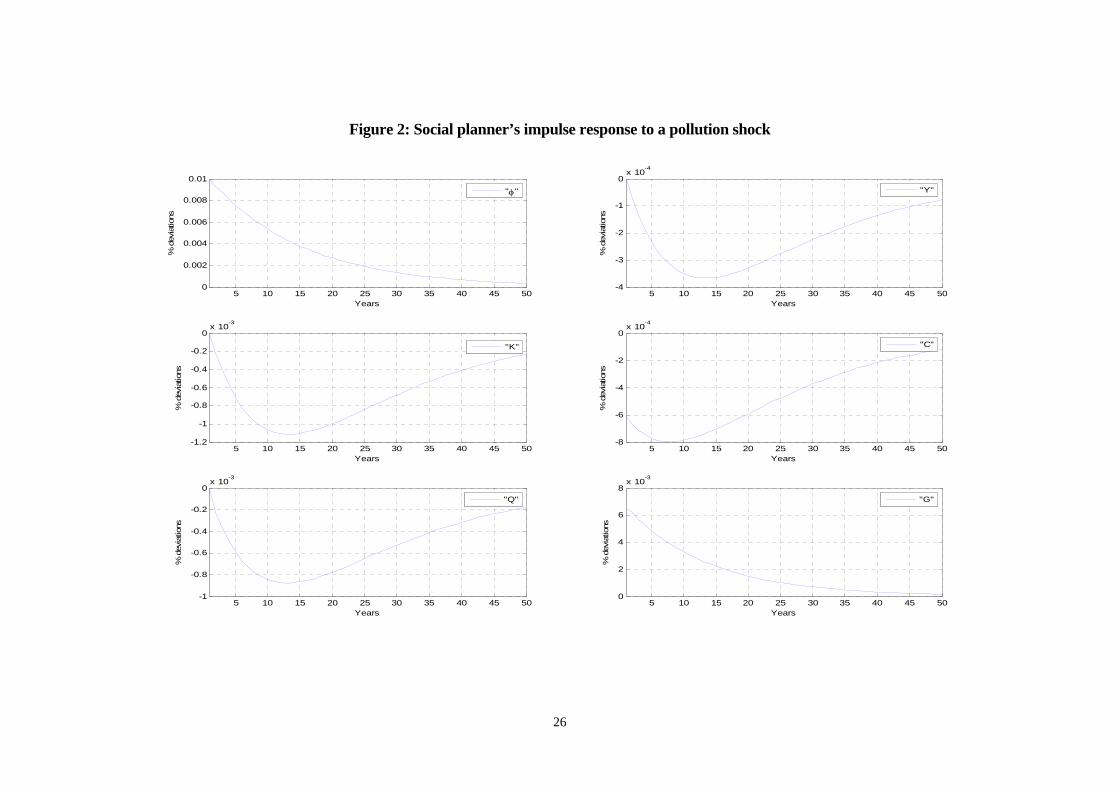
We now present impulse response functions.10 It is convenient to start with the social

planner. The responses of the social planner to a temporary shock to total factor

productivity and the pollution technology are shown in Figures 1 and 2 respectively.

Figures 1 and 2 around here

A positive shock to TFP allows the planner to allocate more resources to clean

up, so that spending on abatement, tG , increases.11 Thus, all allocation decisions

(consumption, tC , capital, 1tK , output, tY , and clean up, tG ) move pro-cyclically.

Notice that, thanks to higher tG , environmental quality, tQ , also improves, despite the

detrimental effect from higher economic activity.

In the case of an adverse pollution shock (a positive shock to t ) things are

different. The planner finds it optimal to increase tG to counter the adverse effect

from a higher t and this is at the cost of lower tC , 1tK and tY . Notice that, despite

the rise in tG , environmental quality, tQ , falls. Thus, while abatement was pro-

cyclical after an economic shock, it is counter-cyclical after an environmental shock.

Also, notice that, while consumption increases by less than output after a positive TFP

shock, as is commonly found in neoclassical models given the consumption

smoothing effect, consumption falls by more than output after an adverse

environmental shock. The latter happens because the planner finds it optimal to

allocate more (less) resources to abatement, despite output falling (increasing) after an

adverse (beneficial) shock to the pollution process.

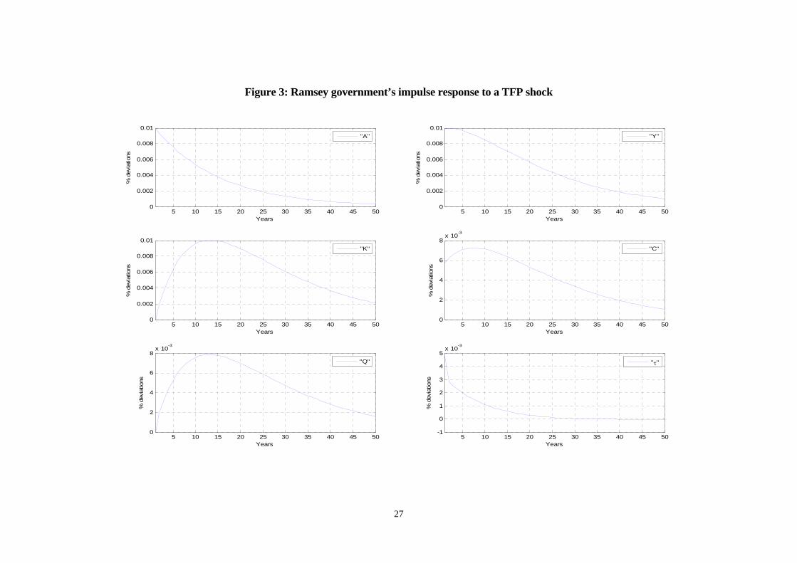
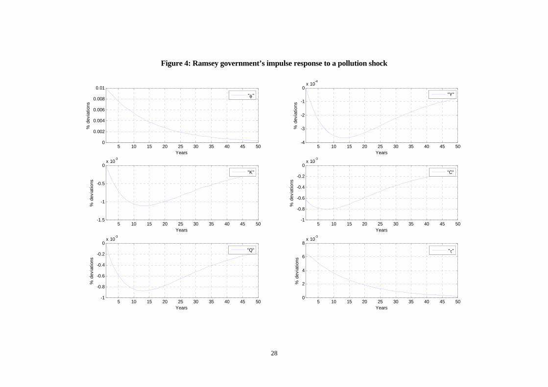
The responses of the Ramsey government to economic and environmental

shocks are shown in Figures 3 and 4 respectively. In both cases, the Ramsey

government finds it optimal to increase the tax rate. In particular, the optimal

environmental tax is pro-cyclical after a TFP shock, while it is counter-cyclical after a

pollution shock. The idea is that, in the former case, the Ramsey government can 10 We report that first- and second-order approximate solutions produce similar impulse responses. This is as in e.g. Schmitt-Grohé and Uribe (2005). The impulse response functions presented here are based on linear approximations around the associated non-stochastic long-run equilibrium. 11 An adverse TFP shock has symmetrically opposite effects.

11

afford a higher tax thanks to better technology, while, in the latter case, the Ramsey

government needs to intervene to counter the adverse environmental shock and this is

at the cost of the real economy. Therefore, in general, the Ramsey government mimics

the behavior of the social planner.

Figures 3 and 4 around here

Notice that our results regarding second-best Ramsey policy reaction to TFP

shocks in the presence of an environmental externality are similar to those obtained by

Heutel (2011). Heutel (2011) also finds that, in the presence of TFP shocks,

environmental quality and the environmental tax should be pro-cyclical. However,

Heutel (2011) does not consider the case of environmental shocks. As we have seen,

in this case, optimal tax policy is counter-cyclical.

5. Allocation and welfare under economic and environmental volatility

We next examine the effect of extrinsic (economic and environmental) volatility on

optimal choices and in turn on social welfare. Extrinsic volatility is measured by the

standard deviation of economic and environmental shocks. Social welfare is measured

by the conditional expectation of the discounted sum of household’s lifetime utility in

(1a-b) above. Our interest is again in examining how optimal responses and social

welfare might differ depending on the source of uncertainty. Also, we look again at

how results in a second-best policy environment differ from those of the social

planner.

To compute the above, we approximate the equilibrium equations in each case

(i.e. in a Ramsey equilibrium with second-best policy and in a social planner

problem), as well as the welfare criterion in (1a-b), to second-order around the

respective non-stochastic steady state solution. Regarding the equilibrium equations,

we compute and simulate their second-order approximations following Schmitt-Grohé

and Uribe (2004). Regarding the welfare criterion, (1a-b), its second-order

approximation is:

1 21 1

00 1 2

1( , )

(1 ) 1 1t

t tt

C QE u C Q

12

1 2 1 21 1 1 12 20 1 2

0

1 1ˆ ˆ ˆ ˆ[ ( ) ( ) ]2 2

tt t t t

t

E C C Q Q C C Q Q

(11)

where, for any variable tx , ˆ ( ) / ln( / )t t tx x x x x x and x is the long-run value of

tx . The values of ˆtC and ˆ

tQ used in (11) are obtained by taking a second-order

approximation to the equilibrium equations of the Ramsey equilibrium with second-

best policy and the social planner problem (see subsection 2.6 and section 3

respectively).

We assume that the economy is initially at its non-stochastic steady state and,

starting from 0t , there are shocks to tA or t , which are the exogenous stochastic

autoregressive processes for production and pollution technologies in (6a)-(6b). We

simulate 300 periods/years, as, because of discounting, later periods do not contribute

to lifetime welfare. We compute the expected first and second moments of the

variables of interest over the lifetime and the expected value of lifetime utility by

calculating the average values of these quantities over 1000 simulations. We do so for

varying degrees of uncertainty, as summarized by the standard deviations of the

production and pollution technologies, a and .

5.1 Optimal policy and welfare under uncertainty

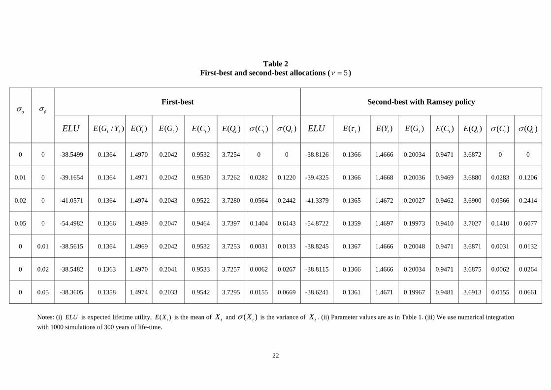
Results for first- and second-best environments are shown in Table 2 under varying

degrees of economic and environmental uncertainty. To understand the consequences

of each type of uncertainty, we study one source of uncertainty at a time. Thus, we

switch off TFP shocks when we consider shocks to the pollution technology, and vice

versa. We report results for three degrees of uncertainty, captured by standard

deviations of 1%, 2% and 5%, for each shock.

Table 2 around here

Table 2 reveals that, in all cases, the Ramsey government achieves economic

outcomes that are inferior to the social planner’s. To contextualize the effects of

uncertainty, we first present results for the non-stochastic steady state, 0a .

The Ramsey tax rate is 13.66%, which is slightly higher than the implicit output share

of the resources earmarked for the protection of environment in the case of the social

planner, which is / 13.64t tG Y .

13

Then, the introduction of uncertainty has two implications at least. First, as

economic uncertainty, a , increases, social welfare falls monotonically in both the

first- and second-best setup. By contrast, the effects of environmental uncertainty, ,

are not clear. In this particular parameterization, a higher lowers welfare at

relatively low levels of volatility but, after a point, welfare appears to increase with

.

Second, although the Ramsey tax rate, t , falls as volatility increases, these

changes in t appear to be rather small in magnitude. As we explain below, this

happens because the Ramsey government also needs to stimulate output as volatility

increases. In other words, although one cannot exclude Ramsey tax cycles (see e.g.

Hagedorn, 2010), our results imply a kind of Barro’s (1979) tax-smoothing effect, in

the sense that the expected mean of the distorting tax rate remains relatively flat

across different volatilities of the exogenous shocks.

In the next subsection, we discuss the incentives behind the above results.

5.2 Precautionary motive and intuition

As the second-order approximation to the utility function in equation (11) indicates,

lifetime utility is affected (positively) by the levels of consumption and environmental

quality, and (negatively) by their standard deviations. Therefore, to understand how

increases in uncertainty affect welfare, Table 2 also presents the first and second

moments of consumption and environmental quality in the social planner and the

Ramsey economy respectively.

As is known from the literature on uncertainty (see e.g. Ljungqvist and

Sargent, 2004, chapter 17, and Aghion and Howitt, 2009, chapter 14), a higher mean-

preserving extrinsic volatility can lead to higher or lower savings, and hence to higher

or lower expected output. The general principle, in the case where higher uncertainty

leads to higher savings and output, is that agents find it optimal to respond to higher

volatility in the exogenous stochastic processes by increasing their precautionary

savings; this works as a buffer against unknown future realizations in general and

unknown future asset returns in particular.12

We again start with the social planner in Table 2. Increases in either type of

uncertainty ( a and ) increase the standard deviation of tC and tQ , which affects

12 Recall that, by using a second-order approximation to equilibrium equations, we allow for the agents’ optimal policies to respond to volatility.

14

welfare negatively. On the other hand, the precautionary behavior is expected to push

the planner to increase asset accumulation resulting in higher levels of consumption

and/or environmental quality in the medium- and long-run. As discussed below, this

depends crucially on the type of the shock hitting the economy.

Recall that there are two “assets” in this model, the stock of physical capital

and the stock of environmental quality. As TFP volatility ( a ) increases, the

precautionary principle suggests that the agent should save more. But, since the return

to physical capital is now relatively more uncertain (because TFP volatility, a , is

higher than environmental volatility, ), the planner finds it optimal to give priority

to environmental protection at the cost of lower consumption. Under the present

parameterization, environmental protection implies higher spending on public

abatement. The adverse effect from a lower tC , in combination with the clear increase

in the volatility of both tC and tQ , imply that the overall welfare is reduced.

On the contrary, as environmental volatility ( ) increases, the precautionary

principle, together with the relatively lower uncertainty in the return to physical

capital, suggest that now the social planner finds it optimal to increase investment in

physical capital and output. Since this allows for more resources to be used for

abatement, and the latter are efficient in improving environmental quality, this

increase in output is good not only for consumption, tC , but also for environmental

quality, tQ . The improvements in both tC and tQ work in opposite direction from the

adverse effects from higher volatility of tC and tQ so the final effect on social

welfare is, in general, not clear. Nevertheless, notice that, in this parameterization,

welfare increases as increases, especially when the degree of environmental

volatility is relatively high. A high value of strongly pushes the agent towards

investing in physical capital, so that the beneficial effects from higher tC and tQ

outweigh the adverse effects from higher volatility.

Inspection of the results in Table 2 reveal that the Ramsey government mimics

the precautionary behavior of the social planer having, however, distorting tax

instruments at its disposal and hence doing worse than the planner. Notice that the

Ramey government finds it optimal to reduce the tax rate, and hence increase output,

as environmental volatility ( ) increases. This is consistent with the precautionary

motive discussed above.

15

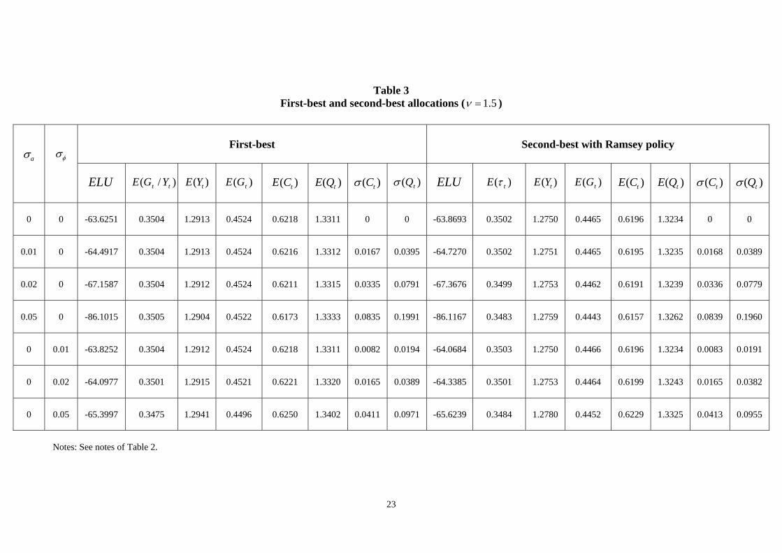
5.3 The importance of the effectiveness of public abatement spending

In this subsection, we check the robustness of our results to changes in the

effectiveness of public abatement technology, (see equations (3) and (4) above). In

the baseline parameterization used so far, we assumed a value for equal to 5

which, in combination with 0.5 and the tax choice made by the Ramsey

government, , implied that the expression was positive in equilibrium. But

what happens when the expression is negative? This would mean that the

beneficial effects from more public abatement spending are outweighed by the

detrimental effects from higher polluting output.13

We now study the effects of lower values of . In particular, we study two

cases. In the first case, we set 1.5 , which means a rather moderate degree of

effectiveness of public abatement policy and, in the second case, we set 0.6 ,

which implies poor effectiveness.14 All other parameter values, including the value of

, remain as before. Results for the two new cases are reported in Tables 3 and 4

respectively.

Tables 3 and 4 around here

Comparison of Tables 2, 3 and 4 reveals that the Ramsey government reacts to

worse public abatement technology (lower ) by increasing the distorting tax rate ( )

in an effort to maintain a positive quantity. This (namely, 0 ) is still

possible in Table 3 where 1.5 , while it is not possible (namely, 0 ) in

Table 4 where 0.6 .15 Thus, when public abatement technology is poor, the

Ramsey government cannot maintain a positive condition any more. In this

case, the precautionary channel does not work under higher economic volatility, so

that both consumption and environmental quality fall. However, the precautionary

channel still works under higher environmental volatility, so that both consumption

and environmental quality rise.

13 We thank one of the referees for pointing this out. 14 Notice that at the level of Decentralized Competitive Equilibrium in subsection 2.5 above, which was for given tax policy, and if we use 31.0 which is close to the EU average for the effective income tax rate, we have 0 for both 5.1 and 6.0 . 15 Similarly, the social planner finds it optimal to increase spending on public abatement as a share of output as decreases. In this section, we focus on the second-best. The results for the social planner are generally similar.

16

Comparison of Tables 2, 3 and 4 also reveals that the higher the equilibrium

value of , the higher the possibility that higher environmental volatility raises

social welfare. Under a lower , the environmental distortion is stronger and this

results in worse economic and environmental outcomes and lower social welfare. In

such a distorted economy, the exogenous shocks have a stronger detrimental effect on

the volatility of endogenous variables. In particular, the standard deviations of both

consumption and environmental quality are much higher under a lower , especially

relative to the mean values of these quantities. In other words, a lower acts as an

amplification mechanism for the exogenous shocks. In turn, this implies that the

welfare gains arising from precautionary behavior are outweighed by the increase in

volatility.

6. Concluding remarks and possible extensions

We compared second-best optimal environmental policy and the resulting allocation

to first-best allocation in a micro-founded dynamic stochastic general equilibrium

model. We focused on the role of uncertainty and showed that the source and

magnitude of extrinsic uncertainty matter to optimal choices and welfare under both

first- and second-best optimal allocations.

We showed that, while higher economic volatility is bad for social welfare, the

effects of higher environmental volatility depend on its size and the effectiveness of

public abatement policy. For instance, when the effectiveness of public abatement

spending is relatively low, the precautionary motive cannot generate strong enough

beneficial effects to outweigh the adverse effects from higher volatility, so that

environmental volatility is also bad for social welfare. We also showed that the

Ramsey environmental tax is pro-cyclical when there is an economic shock, while it is

counter-cyclical when there is an environmental shock. The idea is that when there is

an adverse supply shock, the Ramsey government cuts the tax rate to stimulate the

real economy. On the other hand, when there is a pollution shock, it increases the tax

rate and clean up spending to counter the adverse environmental effect, and this is at

the cost of the real economy.

In this paper, we focused on taxes on polluting output in the second-best case.

An extension could be to study other distorting policy instruments, like pollution

permits and emission targets, and compare the attractiveness of various second-best

17

policies under uncertainty. Another extension could be to study policy and welfare

under model uncertainty, so as to compare optimal and robust environmental policies.

18

APPENDICES

Appendix A: DCE given taxes

The first-order conditions of the individual’s problem include the budget constraint in

(2) and the Euler equation (7b). Using (4)-(5) into (3), we get (7c). All this gives (7a-

c) in the text.

Appendix B: Social planner’s solution

The planner chooses 1 1 0{ , , , }t t t t tC G K Q to maximize (1a-b) subject to:

1 (1 )kt t t t t tK K C G A K (B.1a)

1 (1 )q qt t t t t tQ Q Q A K G (B.1b)

The optimality conditions include the two constraints above and:

1 111 1 1 1 1 1

1

(1 )kt tt t t t t t

t t

u uA K A K

C C

(B.2a)

11

1

qtt t

t

u

Q

(B.2b)

tt

t

u

C

(B.2c)

where 0t is the multiplier associated with (B.1b), 1tt

t

uC

C

and 2tt

t

uQ

Q

.

Using (B.2c) to substitute out t , we get (10a-d) in the text.

19

REFERENCES

Aghion P. and P. Howitt (2009): The Economics of Growth, MIT Press, Cambridge, Mass. Angelopoulos K., G. Economides and A. Philippopoulos (2010): Which is the best environmental policy? Taxes, permits and rules under economic and environmental uncertainty, CESifo, Working Paper, no. 2980, 2010, Munich. Barro R. (1979): On the determination of public debt, Journal of Political Economy, 87, 940-971. Bovenberg A. L. and L. H. Goulder (2002): Environmental taxation and regulation, in Handbook of Public Economics, volume 3, edited by A. Auerbach and M. Feldstein, North-Holland, Amsterdam. Chamley C. (1986): Optimal taxation of capital income in general equilibrium with infinite lives, Econometrica, 54, 607-622. Conesa J. C., S. Kitao and D. Krueger (2009): Taxing capital? Not a bad idea after all!, American Economic Review, 99, 25-48. Congressional Budget Office (2005): Uncertainty in analyzing climate change: policy implications, The Congress of the United States, Congressional Budget Office Paper, January, Washington. Cooley T. F. and G. D. Hansen (1992): Tax distortions in a neoclassical monetary economy, Journal of Economic Theory, 58, 290-316. Economides G. and A. Philippopoulos (2008): Growth enhancing policy is the means to sustain the environment, Review of Economic Dynamics, 11, 207-219. Hagedorn M. (2010): Ramsey tax cycles, Review of Economic Studies, 77, 1042-1071. Heutel G. (2011): How should environmental policy respond to business cycles? Optimal policy under persistent productivity shocks, Review of Economic Dynamics, forthcoming. Jouvet P. A., P. Michel and G. Rotillon (2005): Optimal growth with pollution: how to use pollution permits, Journal of Economic Dynamics and Control, 29, 1597-1609. King R. and S. Rebelo (1999): Resuscitating real business cycles, in Handbook of Macroeconomics, volume 1B, edited by J. Taylor and M. Woodford, North Holland, Amsterdam. Leland H. (1968): Saving and uncertainty: The precautionary demand for saving, Quarterly Journal of Economics, 82, 465-473. Ljungqvist L. and T. Sargent (2004): Recursive Macroeconomic Theory, MIT Press, second edition, Cambridge, Mass.

20

Lucas R. E. (1990): Supply-side economics: an analytical review, Oxford Economic Papers, 42-293-316. Mendoza E. and L. Tesar (1998): The international ramifications of tax reforms: supply side economics in a global economy, American Economic Review, 88, 226-245. Sandmo A. (1970): The effect of uncertainty on saving decisions, Review of Economic Studies, 37, 353-360. Schmitt-Grohé S. and M. Uribe (2004): Solving dynamic general equilibrium models using a second-order approximation to the policy function, Journal of Economic Dynamics and Control, 28, 755-775. Schmitt-Grohé S. and M. Uribe (2005): Optimal fiscal and monetary policy in a medium-scale macroeconomic model: Expanded version, NBER, Working Paper, no. 11417, Cambridge, Mass. Weitzman M. (1974): Prices vs. quantities, Review of Economic Studies, 41, 477-491. Xepapadeas A. (2004): Economic growth and the environment, in Handbook of Environmental Economics volume 3, edited by K. G. Mäler and J. R. Vincent, North-Holland, Amsterdam.

21

Table 1 Baseline parameter values

Parameter

Description Value

capital share in production 0.33

k

Capital depreciation rate 0.1

1 2

curvature parameters in utility function 2

time discount factor 0.97

environment’s weight in utility function 0.4

Q

Environmental quality without pollution 1

q

persistence of environmental quality 0.9

A

long-run total factor productivity 1

a

persistence of total factor productivity 0.933

long-run pollution technology 0.5

persistence of pollution technology 0.933

transformation of spending into units of nature 5, 1.5 and 0.6

22

Table 2 First-best and second-best allocations ( 5 )

Notes: (i) ELU is expected lifetime utility, ( )tE X is the mean of tX

and ( )tX is the variance of tX . (ii) Parameter values are as in Table 1. (iii) We use numerical integration

with 1000 simulations of 300 years of life-time.

a

First-best

Second-best with Ramsey policy

ELU

)/( tt YGE

)( tYE

)( tGE

( )tE C

)( tQE

( )tC

)( tQ

ELU

)( tE

)( tYE

)( tGE

( )tE C

)( tQE

( )tC

)( tQ

0

0

-38.5499

0.1364

1.4970

0.2042

0.9532

3.7254

0

0

-38.8126

0.1366

1.4666

0.20034

0.9471

3.6872

0

0

0.01

0

-39.1654

0.1364

1.4971

0.2042

0.9530

3.7262

0.0282

0.1220

-39.4325

0.1366

1.4668

0.20036

0.9469

3.6880 0.0283

0.1206

0.02 0

-41.0571

0.1364

1.4974

0.2043

0.9522

3.7280

0.0564

0.2442

-41.3379

0.1365

1.4672

0.20027

0.9462

3.6900 0.0566

0.2414

0.05 0

-54.4982

0.1366

1.4989

0.2047

0.9464

3.7397

0.1404

0.6143

-54.8722

0.1359

1.4697

0.19973

0.9410

3.7027 0.1410

0.6077

0

0.01

-38.5615

0.1364

1.4969

0.2042

0.9532

3.7253

0.0031

0.0133

-38.8245

0.1367

1.4666

0.20048

0.9471

3.6871 0.0031

0.0132

0

0.02

-38.5482

0.1363

1.4970

0.2041

0.9533

3.7257

0.0062

0.0267

-38.8115

0.1366

1.4666

0.20034

0.9471

3.6875 0.0062

0.0264

0

0.05

-38.3605

0.1358

1.4974

0.2033

0.9542

3.7295

0.0155

0.0669

-38.6241

0.1361

1.4671

0.19967

0.9481

3.6913

0.0155

0.0661

23

Table 3 First-best and second-best allocations ( 5.1 )

Notes: See notes of Table 2.

a

First-best

Second-best with Ramsey policy

ELU

)/( tt YGE

)( tYE

)( tGE

( )tE C

)( tQE

( )tC

)( tQ

ELU

)( tE

)( tYE

)( tGE

( )tE C

)( tQE

( )tC

)( tQ

0

0

-63.6251

0.3504

1.2913

0.4524

0.6218

1.3311

0

0

-63.8693

0.3502

1.2750

0.4465

0.6196

1.3234

0

0

0.01

0

-64.4917

0.3504

1.2913

0.4524

0.6216

1.3312

0.0167

0.0395

-64.7270

0.3502

1.2751

0.4465

0.6195

1.3235

0.0168

0.0389

0.02

0

-67.1587

0.3504

1.2912

0.4524

0.6211

1.3315

0.0335

0.0791

-67.3676

0.3499

1.2753

0.4462

0.6191

1.3239

0.0336

0.0779

0.05

0

-86.1015

0.3505

1.2904

0.4522

0.6173

1.3333

0.0835

0.1991

-86.1167

0.3483

1.2759

0.4443

0.6157

1.3262

0.0839

0.1960

0

0.01

-63.8252

0.3504

1.2912

0.4524

0.6218

1.3311

0.0082

0.0194

-64.0684

0.3503

1.2750

0.4466

0.6196

1.3234

0.0083

0.0191

0

0.02

-64.0977

0.3501

1.2915

0.4521

0.6221

1.3320

0.0165

0.0389

-64.3385

0.3501

1.2753

0.4464

0.6199

1.3243

0.0165

0.0382

0

0.05

-65.3997

0.3475

1.2941

0.4496

0.6250

1.3402

0.0411

0.0971

-65.6239

0.3484

1.2780

0.4452

0.6229

1.3325

0.0413

0.0955

24

Table 4 First-best and second-best allocations ( 6.0 )

Notes: See notes of Table 2.

a

First-best

Second-best with Ramsey policy

ELU

)/( tt YGE

)( tYE

)( tGE

( )tE C

)( tQE

( )tC

)( tQ

ELU

)( tE

)( tYE

)( tGE

( )tE C

)( tQE

( )tC

)( tQ

0

0

-213.4196

0.64786

0.6523

0.4226

0.2023

0.2739

0

0

-215.1013

0.6965

0.8764

0.61041

0.1990

0.2802

0

0

0.01

0

-213.9065

0.64781

0.6522

0.4225

0.2023

0.2739

0.0020

0.0031

-215.7479

0.6963

0.8763

0.61017

0.1990

0.2802

0.0022

0.0034

0.02

0

-215.4460

0.64769

0.6517

0.4221

0.2023

0.2739

0.0040

0.0062

-217.7755

0.6957

0.8757

0.60922

0.1989

0.2801

0.0043

0.0068

0.05

0

-226.4325

0.64630

0.6480

0.4188

0.2018

0.2736

0.0102

0.0157

-232.2111

0.6914

0.8718

0.60276

0.1982

0.2797

0.0109

0.0170

0

0.01

-219.4311

0.64660

0.6511

0.4210

0.2026

0.2746

0.0099

0.0153

-224.0466

0.6965

0.8771

0.61090

0.1991

0.2808

0.0107

0.0166

0

0.02

-233.6553

0.64284

0.6490

0.4172

0.2037

0.2771

0.0199

0.0307

-246.8265

0.6963

0.8799

0.61267

0.1997

0.2832

0.0212

0.0332

0

0.05

-328.9778

0.62181

0.6383

0.3969

0.2124

0.2969

0.0504

0.0798

-403.9609

0.6937

0.9023

0.62593

0.2048

0.3015

0.0517

0.0830

25

Figure 1: Social planner’s impulse response to a TFP shock

5 10 15 20 25 30 35 40 45 500

0.002

0.004

0.006

0.008

0.01%

dev

iatio

ns

Years

"A"

5 10 15 20 25 30 35 40 45 500

0.002

0.004

0.006

0.008

0.01

% d

evia

tions

Years

"Y"

5 10 15 20 25 30 35 40 45 500

0.002

0.004

0.006

0.008

0.01

0.012

% d

evia

tions

Years

"K"

5 10 15 20 25 30 35 40 45 500

2

4

6

8x 10-3

% d

evia

tions

Years

"C"

5 10 15 20 25 30 35 40 45 500

2

4

6

8x 10-3

% d

evia

tions

Years

"Q"

5 10 15 20 25 30 35 40 45 500

0.005

0.01

0.015

% d

evia

tions

Years

"G"

26

Figure 2: Social planner’s impulse response to a pollution shock

5 10 15 20 25 30 35 40 45 500

0.002

0.004

0.006

0.008

0.01%

dev

iatio

ns

Years

""

5 10 15 20 25 30 35 40 45 50-4

-3

-2

-1

0x 10-4

% d

evia

tions

Years

"Y"

5 10 15 20 25 30 35 40 45 50-1.2

-1

-0.8

-0.6

-0.4

-0.2

0x 10-3

% d

evia

tions

Years

"K"

5 10 15 20 25 30 35 40 45 50-8

-6

-4

-2

0x 10-4

% d

evia

tions

Years

"C"

5 10 15 20 25 30 35 40 45 50-1

-0.8

-0.6

-0.4

-0.2

0x 10-3

% d

evia

tions

Years

"Q"

5 10 15 20 25 30 35 40 45 500

2

4

6

8x 10-3

% d

evia

tions

Years

"G"

27

Figure 3: Ramsey government’s impulse response to a TFP shock

5 10 15 20 25 30 35 40 45 500

0.002

0.004

0.006

0.008

0.01%

dev

iatio

ns

Years

"A"

5 10 15 20 25 30 35 40 45 500

0.002

0.004

0.006

0.008

0.01

% d

evia

tions

Years

"Y"

5 10 15 20 25 30 35 40 45 500

0.002

0.004

0.006

0.008

0.01

% d

evia

tions

Years

"K"

5 10 15 20 25 30 35 40 45 500

2

4

6

8x 10

-3

% d

evia

tions

Years

"C"

5 10 15 20 25 30 35 40 45 500

2

4

6

8x 10

-3

% d

evia

tions

Years

"Q"

5 10 15 20 25 30 35 40 45 50-1

0

1

2

3

4

5x 10

-3

% d

evia

tions

Years

""

28

Figure 4: Ramsey government’s impulse response to a pollution shock

5 10 15 20 25 30 35 40 45 500

0.002

0.004

0.006

0.008

0.01%

dev

iatio

ns

Years

""

5 10 15 20 25 30 35 40 45 50-4

-3

-2

-1

0x 10

-4

% d

evia

tions

Years

"Y"

5 10 15 20 25 30 35 40 45 50-1.5

-1

-0.5

0x 10-3

% d

evia

tions

Years

"K"

5 10 15 20 25 30 35 40 45 50-1

-0.8

-0.6

-0.4

-0.2

0x 10-3

% d

evia

tions

Years

"C"

5 10 15 20 25 30 35 40 45 50-1

-0.8

-0.6

-0.4

-0.2

0x 10

-3

% d

evia

tions

Years

"Q"

5 10 15 20 25 30 35 40 45 500

2

4

6

8x 10

-3

% d

evia

tions

Years

""