FIR Filters for Online Trajectory Planning

with Time- and Frequency-Domain Specifications

Luigi Biagiottia,∗, Claudio Melchiorrib

aDepartment of Information Engineering (DII), University of Modena and ReggioEmilia, Via Vignolese 905, 41100 Modena, Italy

bDepartment of Electronics, Informatics and Systems (DEIS), University ofBologna, Viale Risorgimento 2, 40136 Bologna, Italy

Abstract

In this paper, the use of FIR (Finite Impulse Response) filters for plan-

ning minimum-time trajectories for robots or automatic machines under

constraints of velocity, acceleration, etc. is presented and discussed. In

particular, the relationship between multi-segment polynomial trajectories,

i.e. trajectories composed of several polynomial segments, each one pos-

sibly characterized by constraints on one or more specific derivatives (i.e.

velocity, acceleration, jerk, etc.), and FIR filters disposed in a cascade con-

figuration is demonstrated and exploited in order to design a digital filter for

online trajectory planning. The connection between analytic functions and

dynamic filters allows a generalization of these trajectories, usually obtained

by second- or third-order polynomial functions (e.g. trapezoidal velocity and

double S velocity trajectories), to a generic order with only a modest in-

crease of the complexity. As a matter of fact, the computation of trajectories

∗Corresponding author. Tel.:+390592056315; fax:+390592056329.Email addresses: luigi.biagiotti@unimore.it (Luigi Biagiotti),

claudio.melchiorri@unibo.it (Claudio Melchiorri)

Preprint submitted to Control Engineering Practice May 18, 2012

with higher degree of continuity simply requires additional FIR filters in the

chain. Moreover, the modular structure of the planner provides a direct fre-

quency characterization of the motion law. In this way, it is possible to define

the trajectories by considering constraints expressed in the frequency-domain

besides the classical time-domain specifications, such as bounds on velocity,

acceleration, and so on. Two examples illustrate the main features of the

proposed trajectory planner, in particular with respect to the problems of

multi-point trajectories generation and residual vibrations suppression.

Keywords: Trajectory planning, Multi-segment trajectories, Shaping

filters, Digital filters

1. Introduction

The growing need of planning trajectories online has led to the develop-

ment of a number of filters able to produce motion profiles with the desired

degree of smoothness simply starting from rough reference signals, such as

step functions, which set the desired final position. Examples of these tra-

jectory planners have been presented e.g. in Zanasi et al. (2000); Zanasi and

Morselli (2003) or, more recently, in Zheng et al. (2009), where minimum-

time trajectory planners with bounds on velocity, acceleration, and jerk have

been proposed. Basically, these planners are composed by a chain of integra-

tors (whose output represents the desired trajectory) with a proper nonlinear

feedback controller so that the reference input is tracked in the fastest pos-

sible manner while remaining compliant with the given constraints. These

trajectory generators allow to consider even asymmetric positive and negative

limits, that can be changed in runtime. Moreover, the filters can be applied

2

to reference signals different from simple step functions. In this case, the

output follows the input with no changes and no delay if the input is com-

pliant with the constraints, otherwise the output tracks the input at best

under the imposed limits. This kind of filters has been successfully applied

in the robotics field, in order to cope with the speed limits that character-

ize mobile robots, see Bonfe and Secchi (2010), and to take into account

the torque limits affecting mechanical manipulators, see Gerelli and Guarino

Lo Bianco (2008), besides the usual kinematic bounds on velocity and accel-

eration, as in Gerelli and Guarino Lo Bianco (2009). However, although very

versatile, these trajectory planners are characterized by an high complexity

and therefore are rather demanding from a computational point of view. A

simpler solution to the problem of online trajectory planning and trajectory

smoothing consists in the application to the reference commands, provided

by a coarse interpolator, of one or more linear filters. In motion control of

CNC machines, FIR (Finite Impulse Response) filters are generally adopted

because their efficiency and the possibility to be easily implemented by hard-

ware. The acceleration/deceleration circuit proposed in Nozawa et al. (1985)

is nothing but a moving average filter that produces as output the mean of

the last n input samples (of the reference velocity). In Kim et al. (1994)

the convolution of the reference signal, representing the velocity along the

desired path, with various kinds of digital filters is proposed for properly

shaping the acceleration/deceleration profile; again, a single moving average

filter is used to obtain a constant acceleration but it is recognized that a

chain of such filters would make the motion smoother and smoother. In Jeon

and Ha (2000) the use of a single FIR filter for smoothing a given feedrate

3

signal is generalized to any kind of acceleration profile, by properly comput-

ing coefficients of the filter. A similar approach, but based on continuous

filters, is represented by the so-called input shaping, that consists in filtering

the reference input by convolving it with a train of impulses in order to form

a new command that causes little or no vibrations on the mechanical plant,

see Singer and Seering (1990); Tuttle and Seering (1994). This technique has

been adopted for reduction of crane oscillations, see Hong and Hong (2004),

control of industrial machines like XY stages, see Fortgang et al. (2005), vi-

bration suppression in flexible robotic arms, see Magee and Book (1998). For

a comprehensive overview about input shaping techniques refer to Singhose

(2009).

In this paper, the advantages of the filtering techniques, that allow to prop-

erly shape the frequency spectrum of a motion law, are combined with the

features of multi-segment trajectories, whose parameters are generally de-

fined with the only purpose of making the trajectories compliant with given

bounds on velocity, acceleration, jerk, etc. The key point is the equivalence

between time-optimal multi-segment polynomial trajectories with constraints

on the first n derivatives and the output of a chain of nmoving average filters.

Therefore, in this case the filters are not used for making a given trajectory

smoother but for online generating a trajectory starting from initial and final

positions, similarly to feedback controlled planners. The equivalence between

dynamic filters and trajectories expressed by analytic functions provides an

immediate characterization of the motion from a spectral point of view. This

is of great importance when it is necessary to plan a trajectory for systems

which are critical with respect to the problem of vibrations (Lambrechts

4

et al., 2005; Barre et al., 2005), since it is possible to set the parameters of

the trajectory on the basis of the frequency response of the plant.

The paper is organized as follows. In Sec. 2 the equivalence between multi-

segment trajectories defined by analytic functions and the output of chains

of finite memory filters is demonstrated. On the basis of this equivalence,

the formulae relating the characteristic parameters of the filters and the limit

values of velocity, acceleration, jerk, etc. are deduced and the spectrum of a

generic trajectory of order n is obtained. In Sec. 3 the continuous-time fil-

ters are approximated by discretization with banks of moving average filters

that can be directly implemented on digital controllers. Section 4 illustrates,

by means of some numerical examples, the advantages of the proposed fil-

ter for generating multi-point trajectories and planning time-optimal motion

profiles in those applications in which, besides bounds on the magnitude

of trajectory derivatives, constraints in the frequency domain are present.

Concluding remarks are provided in the last section.

2. Multi-segment trajectories and dynamic filters

Multi-segment trajectories are motion laws composed by several tracts,

each one characterized by a specific analytical expression, properly joined in

order to guarantee the desired degree of smoothness. In particular, time-

optimal trajectories under constraints of velocity, acceleration, jerk, etc. are

characterized by segments in which the velocity, the acceleration, and higher

derivatives (depending on the required order of continuity) are saturated to

the maximum allowed value. By imposing constraints on the first n deriva-

tives one obtains a trajectory q(t) of class Cn−1, that is with the first n − 1

5

hu(t) qn(t)q1(t) q2(t) qn−1(t)1− e−sT1

sT1

1− e−sT2

sT2

1− e−sTn

sTn

Figure 1: System composed by n filters for the computation of an optimal trajectory of

class Cn−1.

derivatives that are continuous, while the n-th derivative q(n)(t) is a piece-

wise constant function whose values belong to the set {q(n)min, 0, q(n)max}. The

number n is called order of the trajectory. Typical examples of multi-segment

trajectories are the well known “trapezoidal velocity” trajectory and the

“double S velocity” trajectory, of order two and three respectively. With the

additional condition of symmetric constraints:

q(i)min = −q(i)max, i = 1, . . . , n

one can show that such a kind of trajectories can be obtained by filtering a

step input with a cascade of n dynamic filters, each one characterized by the

transfer function

Mi(s) =1

Ti

1− e−sTi

s(1)

where the parameter Ti (in general different for each filter composing the

chain) is a time length, see Fig. 1. The possibility of obtaining time-optimal

trajectories with the system of Fig. 1 fed by step input functions can be

proved by exploiting a property of the convolution product (denoted with ∗)on the differentiation, i.e.

d

dt(f ∗ g) = df

dt∗ g = f ∗ dg

dt. (2)

Consider the case of a single filter with a step input of generic magnitude

6

q0(t) m1(t) → q1(t) m2(t) → q2(t) m3(t) → q3(t)

Position

qi(t)t

h

tT

1T1

→

t tT2

1T2

→

t tT3

1T3

→

t

d

dt

Velocity

q(1)

i(t)

t tT1

1T1

→

tT1 tT2

1T2

→

t tT3

1T3

→

t

d

dt

Acceleration

q(2)

i(t) tT1 tT2

1T2

→ T1T2 T1 + T2 tT3

1T3

→ t

d

dt

Jerk

q(3)

i(t) T1T2 T1 + T2 tT3

1T3

→ t

1

∗

∗∗

∗∗∗

∗∗∗

∗∗∗

∫ t

0

dτ

∫ t

0

dτ

∫ t

0

dτ

∫ t

0

dτ

∫ t

0

dτ

∫ t

0

dτ

h δ(t) =

Figure 2: Relationships among the profiles of trajectories obtained by iterated averaging

operations. Note that in the first row the algebraic relation qi(t) = qi−1(t)∗mi(t), i = 1, 2, 3

is reported, while in the remaining rows a pictorial representation of the relationship among

the trajectories of different orders and their derivatives is shown.

h, i.e. hu(t), being u(t) the unit step function

u(t) =

1, t ≥ 0

0, t < 0.

In this case the output trajectory can be computed as

q1(t) = hu(t) ∗m1(t) (3)

where

mi(t) = L−1{Mi(s)} =1

Ti

(

u(t)− u(t− Ti))

, i = 1

is the impulse response corresponding to Mi(s). Note that mi(t) is a rectan-

gular function of duration Ti and magnitude 1/Ti, see Fig. 2. This implies

7

that, as well known, for any choice of Ti the area of the rectangular func-

tion is unitary, and accordingly the static gain of the corresponding function

Mi(s) is unitary as well:

Mi(0) =

∫ ∞

0

mi(τ) dτ = 1.

By applying (2) to (3) one obtains

q(1)1 (t) = hu(1)(t) ∗m1(t)

= h δ(t) ∗m1(t) = hm1(t)

where δ(t) is the unit impulse function. Therefore, by adopting a single

filter M1(s) fed by a step function of amplitude h, the output consists in

a trajectory q1(t) whose velocity has a rectangular profile with magnitude

v = h/T1. Then, it is immediate to obtain the value of the parameter T1

which permits to impose a desired (limit) value of the velocity1:

v =|h|T1

= q(1)max → T1 =|h|q(1)max

. (4)

Accordingly, when a step input of amplitude h is applied, the output ofM1(s)

will change from the initial to the final value (given by h) with a linear profile

whose duration is exactly T1.

If one adds a second filter M2(s), characterized by the parameter T2, the

1Since T1 must be positive, it is necessary to consider the absolute value of the dis-

placement. In fact, if h < 0 the constant velocity will be equal to the minimum value,

that is

v =h

T1= q

(1)min = −q(1)max → T1 =

−h

q(1)max

=|h|q(1)max

.

8

resulting trajectory is

q2(t) = q1(t) ∗m2(t)

= hu(t) ∗m1(t) ∗m2(t). (5)

Therefore, the first derivative is

q(1)2 (t) = q

(1)1 (t) ∗m2(t) (6)

= hm1(t) ∗m2(t)

and, by taking into account that

m(1)1 (t) =

1

T1

(

δ(t)− δ(t− T1))

it is possible to deduce the second derivative

q(2)2 (t) = hm

(1)1 (t) ∗m2(t)

=h

T1

(

δ(t)− δ(t− T1))

∗m2(t)

= v(

m2(t)−m2(t− T1))

which is composed by two rectangular functions, one positive and one neg-

ative, of magnitude a =v

T2

and duration min{T1, T2}. Therefore the maxi-

mum value of the acceleration can be freely set by imposing

a =v

T2

= q(2)max → T2 =v

q(2)max

=q(1)max

q(2)max

. (7)

Since the static gain of both M1(s) and M2(s) is unitary, the final value of

the response of M1(s)·M2(s) to a step input of magnitude h remains h. The

system output q2(t) reaches such a value with a trapezoidal velocity profile

obtained by integrating q(2)2 (t).

9

The maximum acceleration of the trajectory is q(2)max, and the velocity is still

limited by q(1)max. In fact, by defining for a generic function f(t)

peak(

f(t))

= maxt≥0

|f(t)|

from (6) one can prove that

peak(

q(1)2 (t)

)

≤ peak(

q(1)1 (t)

)

·∫ ∞

0

|m2(τ)|dτ

≤ peak(

q(1)1 (t)

)

= q(1)max (8)

being∫∞

0|m2(τ)|dτ =

∫∞

0m2(τ)dτ = 1 since m2(t) ≥ 0, ∀t. In this case, if

T1 ≥ T2 then the maximum velocity q(1)max is actually reached, i.e. peak

(

q(1)2 (t)

)

=

q(1)max and q2(t) is a minimum-time trajectory compliant with the given bounds

q(i)max, i = 1, 2. Conversely, if T1 < T2 then peak

(

q(1)2 (t)

)

= |h|T2

< |h|T1

= q(1)max,

and the trajectory, that still meets the proposed constraints, is not of mini-

mum duration. In Fig. 3, the trapezoidal trajectories obtained for two differ-

ent displacements h and with the same limits q(1)max and q

(2)max that guarantee

T1 = 0.08 ≥ T2 = 0.05 in case (a) and T1 = 0.02 < T2 = 0.05 in case (b) are

reported. Note in particular, that when T1 < T2, the roles of the two time

constants Ti are switched (in the sense that the duration of the acceleration

period is T1 and the maximum velocity is h/T2).

The total duration of the trajectory q2(t) is given by the sum of the durations

of the impulse responses of M1(s) and M2(s), i.e.

Ttot = T1 + T2.

Note that the maximum velocity q(1)max is actually reached if and only if

T2 ≤1

2Ttot =

1

2(T1 + T2) ⇔ T2 ≤ T1.

10

0 0.05 0.1 0.15−5000

0

5000

0

100

200

3000

5

10

15

20

q 2(t)

q(1)

2(t)

q(2)

2(t)

t

T1T2 T1 + T2

h/T1

0 0.01 0.02 0.03 0.04 0.05 0.06 0.07 0.08−5000

0

5000

0

100

200

3000

1

2

3

4

5

q 2(t)

q(1)

2(t)

q(2)

2(t)

t

T1 T2 T1 + T2

h/T2

(a) (b)

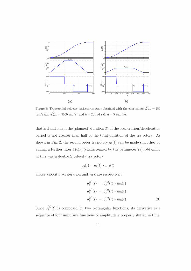
Figure 3: Trapezoidal velocity trajectories q2(t) obtained with the constraints q(1)max = 250

rad/s and q(2)max = 5000 rad/s2 and h = 20 rad (a), h = 5 rad (b).

that is if and only if the (planned) duration T2 of the acceleration/deceleration

period is not greater than half of the total duration of the trajectory. As

shown in Fig. 2, the second order trajectory q2(t) can be made smoother by

adding a further filter M3(s) (characterized by the parameter T3), obtaining

in this way a double S velocity trajectory

q3(t) = q2(t) ∗m3(t)

whose velocity, acceleration and jerk are respectively

q(1)3 (t) = q

(1)2 (t) ∗m3(t)

q(2)3 (t) = q

(2)2 (t) ∗m3(t)

q(3)3 (t) = q

(3)2 (t) ∗m3(t). (9)

Since q(2)2 (t) is composed by two rectangular functions, its derivative is a

sequence of four impulsive functions of amplitude a properly shifted in time,

11

see Fig. 2. Therefore, from (9) it descends that q(3)3 (t) is composed by four

rectangular functions of amplitude j = a/T3 and accordingly it is possible to

select T3 on the basis of the desired value of the jerk:

j =a

T3

= q(3)max → T3 =a

q(3)max

=q(2)max

q(3)max

. (10)

Moreover, by the same argument as in (8) one can prove that

peak(

q(2)3 (t)

)

≤ peak(

q(2)2 (t)

)

= q(2)max (11)

peak(

q(1)3 (t)

)

≤ peak(

q(1)2 (t)

)

≤ peak(

q(1)1 (t)

)

= q(1)max. (12)

In particular, if the tract with constant jerk is at most half of the accelera-

tion/deceleration period, that is

T3 ≤1

2(T2 + T3) ⇔ T3 ≤ T2, (13)

in (11) the sign equal holds true and the maximum acceleration q(2)max is ac-

tually reached by the third order trajectory q3(t). Analogously, if the accel-

eration/deceleration period does not exceed half of the total duration of the

trajectory, i.e.

T2 + T3 ≤1

2(T1 + T2 + T3) ⇔ T2 + T3 ≤ T1 (14)

then peak(

q(1)3 (t)

)

= peak(

q(1)2 (t)

)

(and obviously peak(

q(1)2 (t)

)

= peak(

q(1)1 (t)

)

since (14) implies T2 ≤ T1), therefore the trajectory q3(t) reaches the max-

imum velocity q(1)max. If, both conditions (13) and (14) are met, the velocity

and the acceleration reach the maximum values q(i)max, and q3(t) is a minimum-

time trajectory. Conversely, when one (or both) of the two conditions is not

true, the trajectory is compliant with the given bounds but it is not time-

optimal. In Fig. 4 the possible situations are exemplified. In the case (a) the

12

0 0.05 0.1 0.15 0.2 0.25 0.3−10

−5

0

5x 10

4−5000

0

5000

0

100

200

3000

10

20

30

40

q 3(t)

q(1)

3(t)

q(2)

3(t)

q(3)

3(t)

t0 0.05 0.1 0.15 0.2

−15

−10

−5

0

5

x 104

−2000

0

2000

0

100

200

3000

5

10

15

20

q 3(t)

q(1)

3(t)

q(2)

3(t)

q(3)

3(t)

t0 0.02 0.04 0.06 0.08 0.1 0.12 0.14

−15

−10

−5

0

5

x 104−5000

0

5000

0

100

200

3000

1

2

3

4

5

q 3(t)

q(1)

3(t)

q(2)

3(t)

q(3)

3(t)

t

(a) (b) (c)

Figure 4: Double S velocity trajectories q3(t) obtained with h = 40 rad, q(1)max = 250 rad/s,

q(2)max = 5000 rad/s2, q

(3)max = 50000 rad/s3 (a), h = 20 rad, q

(1)max = 250 rad/s, q

(2)max =

3000 rad/s2, q(3)max = 80000 rad/s3 (b), h = 5 rad, q

(1)max = 250 rad/s, q

(2)max = 5000 rad/s2,

q(3)max = 80000 rad/s3 (c).

time constants defining the three filters and computed on the basis of the

given limit values, are

T1 = 0.16 s, T2 = 0.05 s, T3 = 0.1 s,

therefore (13) is false while (14) is true. Consequently, the maximum ac-

celeration actually reached is not q(2)max = 5000 rad/s2 but peak

(

q(2)3 (t)

)

=

2500 rad/s2. The case (b) is dual to (a). As a matter of fact

T1 = 0.08 s, T2 = 0.0833 s, T3 = 0.0375 s,

and therefore (13) is true and (14) is false. In this situation, the desired max-

imum acceleration is reached, while the maximum velocity is peak(

q(1)3 (t)

)

=

13

=∗

q(3)2 (t)

q(3)3 (t)

m3(t)

t tt T1T1 T2T2 T3 T1 + T2T1 + T2

q(3)max

−q(3)max

Figure 5: Jerk profile of a third order trajectory q3(t) characterized by the time constants

Ti, i = 1, 2, 3 with T1 − T2 < T3.

216.65 < 250 rad/s. In the example reported in Fig. 4(c), that corresponds

to

T1 = 0.02 s, T2 = 0.05 s, T3 = 0.0625 s,

both conditions (13) and (14) are not met and the trajectory does not reach

neither the maximum velocity nor the maximum acceleration. Moreover, in

the case T1 < T2 + T3, that is in the examples of Fig. 4(b) and Fig. 4(c), the

jerk exceeds the given bound. This is due to the fact that the jerk profile,

obtained by convoluting a sequence of four impulsive functions by the impulse

response of the third filter m3(t), is given by the superimposition of the single

responses. Therefore if the distance between the application time-instants of

two impulses with the same sign is smaller than the duration of m3(t), the

responses are partially overlapped and produce a jerk profile that reaches a

level twice the desired value, see Fig. 5.

The procedure shown so far can be iterated by adding further filters

Mi(s). In the general case, the expression of the minimum-time trajectory

14

compliant with given constraints on the first n derivatives, and therefore of

order n, is

qn(t) = hu(t) ∗m1(t) ∗ . . . ∗mn−1(t) ∗mn(t) (15)

or with a recursive formulation

qn(t) = qn−1(t) ∗mn(t) (16)

where q0(t) = hu(t). As already pointed out, the smoothness of the trajec-

tory, that is the order of continuous derivatives, is strictly tied to the number

of filters composing the chain. If one considers n filters, the resulting trajec-

tory will be of class Cn−1. By increasing the smoothness of the trajectory,

the duration augments as well. As a matter of fact the total duration of a

trajectory planned by means of n dynamic systems Mi(s) is given by the sum

of the lengths of the impulse response of each filter, i.e.

Ttot = T1 + T2 + . . .+ Tn.

The parameters Ti can be set with the purpose of imposing desired bounds

on velocity, acceleration, jerk and higher derivatives, i.e.

|q(i)n (t)| ≤ q(i)max, i = 1, . . . , n (17)

by assuming

T1 =|h|q(1)max

(18)

Ti =q(i−1)max

q(i)max

, i = 2, . . . , n

with the constraints

Tj ≥ Tj+1 + . . .+ Tn, j = 1, . . . , n− 1. (19)

15

that guarantee that the trajectory, compliant with (17), is of minimum du-

ration.

2.1. Role of the constraints on Ti and optimality of the trajectory

The trajectory planner composed by n filters Mi(s) guarantees an output

trajectory qn(t) compliant with the given constraints and of minimum du-

ration if such constraints lead to time constants Ti that verify (19). In this

manner the n-th derivative of qn(t) is composed by 2n−1 distinct rectangular

functions mn(t) properly shifted in time. The limit case occurs when two of

these functions are contiguous (but not overlapped). Note that

q(n)n (t) = q(n)n−1(t) ∗mn(t)

where (if the n − 1-th trajectory is time optimal) q(n)n−1 is a train of 2n−1

impulses. The condition (19), that can be rewritten as

Tj − Tj+1 − . . .− Tn−1 ≥ Tn, j = 1, . . . , n− 1, (20)

means that the distance between adjoining impulses composing q(n)n−1 must

be greater than the duration Tn of mn(t). In fact, Tj − Tj+1 − . . . − Tn−1,

j = 1, . . . , n− 1 represents the distances between pairs of impulses.

As already mentioned, if (19) is not true the trajectory qn(t), obtained as

output of the cascade of n filters, is not of minimum duration. In particular,

if the inequality (19) is false for a given index j, i.e.

Tj < Tj+1 + . . .+ Tn,

the trajectory is characterized by

peak(

q(j)n (t))

< q(j)max,

16

that is the limit value of the j-th derivative is not reached. In this case, by

reducing the value of q(j)max (that remains therefore compatible with the initial

constraint) it is possible to increase Tj = q(j−1)max /q

(j)max until

Tj = Tj+1 + . . .+ Tn. (21)

Note that, a reduction of q(j)max implies that Tj+1 is also reduced and it may

happens that (19) becomes false for j + 1.

In the general case in which inequalities (19) are false for k values of the

index j, namely j1, j2, . . . , jk, it is necessary to reduce q(ji)max, i = 1, . . . , k until

Tji= Tji+1 + . . .+ Tn, i = 1, . . . , k (22)

and checking if (19) for the remaining index j still holds true. In general,

a closed-form solution of the problem cannot be found since many different

situations may arise, but the cases n = 2 and n = 3 may be easily handled.

In particular, for trapezoidal velocity trajectories generated by FIR filters

(n = 2), when T1 < T2, from T1 = |h|

q(1)max

= q(1)max

q(2)max

= T2, one may deduce the

value of the maximum velocity that makes the trajectory time-optimal, that

is

q(1)max =

√

|h| q(2)max < q(1)max. (23)

The 2-nd order trajectory obtained with the same conditions of example

in Fig. 3(b) but with the maximum velocity computed according to (23)

is shown in Fig. 6, where it is compared with the original motion profile.

Note that, the trajectory is still compliant with all the constraints, but it

is considerably shorter than the motion profile obtained by simply applying

(18) on the initial data (without modifying the maximum velocity).

17

0 0.01 0.02 0.03 0.04 0.05 0.06 0.07 0.08−5000

0

5000

0

100

200

3000

1

2

3

4

5

q 2(t)

q(1)

2(t)

q(2)

2(t)

t

T1 = T2 T1 + T2

q(1)max

Figure 6: Trapezoidal velocity trajectory q2(t) obtained with the same conditions of ex-

ample in Fig. 3(b) but with the constraint q(1)max = 158.11 rad/s that leads to T1 = T2 =

0.0316 s.

In the case n = 3, it may happen that

T1 < T2 + T3 ⇔ |h|q(1)max

<q(1)max

q(2)max

+q(2)max

q(3)max

(24)

or

T2 < T3 ⇔ q(1)max

q(2)max

<q(2)max

q(3)max

(25)

and it is therefore necessary to modify the maximum value of the velocity or

of the acceleration in order to make the two inequalities false. For instance,

if (24) and (25) are both true, the optimal values of the maximum velocity

and accelerations are

q(1)max =

|h|2/3 q(3)max

1/3

22/3

q(2)max =

|h|1/3 q(3)max

2/3

21/3.

(26)

18

0 0.05 0.1 0.15 0.2 0.25 0.3−10

−5

0

5x 10

4−5000

0

5000

0

100

200

3000

10

20

30

40

q 3(t)

q(1)

3(t)

q(2)

3(t)

q(3)

3(t)

t0 0.05 0.1 0.15 0.2

−15

−10

−5

0

5

x 104

−2000

0

2000

0

100

200

3000

5

10

15

20

q 3(t)

q(1)

3(t)

q(2)

3(t)

q(3)

3(t)

t0 0.02 0.04 0.06 0.08 0.1 0.12 0.14

−15

−10

−5

0

5

x 104−5000

0

5000

0

100

200

3000

1

2

3

4

5

q 3(t)

q(1)

3(t)

q(2)

3(t)

q(3)

3(t)

t

(a) (b) (c)

Figure 7: Double S velocity trajectories q3(t) obtained under the same constraints of

examples in Fig. 4, but with q(2)max = 3535.5 rad/s2 (a), q

(1)max = 195.07 rad/s (b) and

q(1)max = 79.37 rad/s, q

(2)max = 2519.8 rad/s2 (c).

If only (24) is valid

q(1)max =1

2

−q(2)max

2

q(3)max

+

√

√

√

√

q(2)max

4

q(3)max

2 + 4|h|q(2)max

(27)

while, if only (25) holds true

q(2)max =

√

q(1)max q

(3)max. (28)

With these values used for the computation of parameters Ti, one obtains

the minimum-time double S velocity trajectory compliant with the initial

constraints. In Fig. 7, the trajectories of the examples reported in Fig. 4

are compared with those obtained by modifying the maximum velocity or

acceleration according to the procedure above illustrated. In particular, the

19

values of the filters parameters are

T1 = 0.16 s, T2 = 0.0707 s, T3 = 0.0707 s

in case (a),

T1 = 0.1025 s, T2 = 0.0650 s, T3 = 0.375 s

in case (b),

T1 = 0.063 s, T2 = 0.0315 s, T3 = 0.0315 s

in case (c). Note that the duration of the trajectory in Fig. 7(b) is higher

than the time-length of the original trajectory since the value of velocity pro-

vided by (27), that is q(1)max = 195.07 rad/s, is lower than the peak velocity

of the initial trajectory, i.e. peak(

q(1)3 (t)

)

= 216.65 rad/s. In this case the

modification of the time constants Ti makes the trajectory a true double S

trajectory, with the jerk q(3)(t) ∈ {−q(3)max, q

(3)max}, but it is worth noticing that

in many applications the bound on the jerk is not due to physical limitations

of the actuation system or of the load but it is a means to reduce oscillations

and residual vibrations on the system. Therefore the limit values of jerk are

a recommendation rather than a strict constraint. Moreover, as shown in

Sec. 4.2, residual vibrations are related to the frequency spectrum of the tra-

jectory (that depends on the parameters Ti) and not to the magnitude of jerk

and other derivatives. For these reasons, in many cases a shorter duration of

the trajectory may be preferable to a strict compliance with the bound on

the jerk.

20

In general, when the j-th constraint on Ti, expressed by (19), is not met,

one should act on q(j)max. This modification leads to a reduction of the total

duration of the trajectory only if the initial values of Ti, i = j . . . n verify the

inequality

(Tj − Tj−1)2 > (Tj−2 + . . . Tn)

2. (29)

Therefore, when (29) is not true it may be convenient to maintain the initial

Ti, even if, strictly speaking, the resulting profile cannot be considered an

optimal multi-segment trajectory, according to the usual definition. Consider

that, although (19) is false, the bounds on q(i)max, i = 1, . . . , n− 1 are met in

any case and only q(n)max is overcome.

2.2. Derivatives of a generic trajectory

A trajectory generator should provide not only the position profile of

the trajectory but also the related profiles of velocity, acceleration, jerk, etc.

which are needed to implement e.g. feed-forward actions on the controlled

system.

The computation of the derivatives of a trajectory of generic order n, that

is obtained by a cascade of n filters, is straightforward by considering the

definition (15) and the property of convolution product (2). In fact,

q(1)n (t) = qn−1(t) ∗m(1)n (t)

= qn−1(t) ∗1

Tn

(

δ(t)− δ(t− Tn))

(30)

=1

Tn

(

qn−1(t)− qn−1(t− Tn))

.

21

hu(t) qn(t)q1(t) qn−1(t)qn−2(t)

q(1)n (t)

q(2)n (t)

q(n)n (t)

q(1)n−1(t)

q(n−1)n−1 (t)q

(n−2)n−2 (t)q

(1)1 (t)

1− e−sT1

sT1

1− e−sTn−1

sTn−1

1− e−sTn

sTn

1− e−sTn

Tn

1− e−sTn

Tn

1− e−sTn

Tn

1− e−sTn−1

Tn−1

1− e−sTn−1

Tn−1

1− e−sT1

T1

Figure 8: System composed by n filters for the computation of an optimal trajectory of

class Cn−1 and of all the derivatives of order i = 1, . . . , n.

The generic derivative of k-th order, can be calculated in a recursive manner

as

q(k)n (t) =1

Tn

(

q(k−1)n−1 (t)− q

(k−1)n−1 (t− Tn)

)

(31)

with q(0)n−k(t) = qn−k(t). Figure 8 shows the block-scheme representation of

the filter for the computation of the trajectory and its derivatives, obtained

by iterating and Laplace transforming (31). Note that the filter of Fig. 8 gives

a closed form expression (in terms of Laplace transform) of the derivatives

and does not simply provide their numerical value.

2.3. Frequency characterization of the trajectory/filter

The spectrum of the trajectory can be readily deduced by considering its

expression in terms of Laplace transform (directly obtained from (15)), i.e.

Qn(s) =h

s·M1(s) ·M2(s) · . . . ·Mn(s). (32)

22

As a matter of fact, as it is well known, the Fourier transform of qn(t) im-

mediately descends from Qn(s), being the restriction to the imaginary axis,

i.e. Qn(jω). Therefore, the closed form expression of Qn(jω) is given by the

products of the Fourier signal corresponding to the input hu(t) and of the

frequency responses of the filters composing the trajectory generator:

Qn(jω) =h

jω·M1(jω) ·M2(jω) · . . . ·Mn(jω)

where

Mi(jω) =1

Ti

1− ejωTi

jω

= e−jωTi2sin

(

ωTi

2

)

ωTi

2

. (33)

Since the frequency characterization of the trajectories, including their deriva-

tives and, in particular, the acceleration, is a useful tool to predict vibratory

phenomena in the systems to which the trajectories are applied (Biagiotti

and Melchiorri, 2008), it is necessary to obtain the expression of the spec-

trum of the generic k-th derivative of qn(t). Because of the properties of

Laplace transforms, this result is straightforward. As a matter of fact, the

Laplace transform of q(k)n (t) is given by

Q(k)n (s) = skQn(s)

and therefore the expression of the spectrum of q(k)n (t) is

Q(k)n (jω) = (jω)k ·Qn(jω)

= h· (jω)k−1·M1(jω) ·M2(jω) · . . . ·Mn(jω).

In conclusion, the amplitude spectrum of qn(t) and its derivatives, i.e. |Q(k)n (jω)|,

is given by the product of two main elements:

23

ω/ωi0

1

1 2 3 4 5

∣ ∣ ∣ ∣

sinc

(

ω ωi

)∣ ∣ ∣ ∣

Figure 9: Magnitude of the frequency response of the filter Mi(s).

• a power of ω, i.e. ωk−1, being k the order of the derivative;

• the (magnitude of the) frequency response of the chain of n filters

Mi(s).

The frequency response of the cascade of filters is the product of the single

frequency responses Mi(jω), i = 1, . . . , n, whose magnitude is

|Mi(jω)| =∣

∣

∣

∣

∣

sin(

ωTi

2

)

ωTi

2

∣

∣

∣

∣

∣

=

∣

∣

∣

∣

sinc

(

ω

ωi

)∣

∣

∣

∣

where sinc(·) denotes the normalized sinc function defined as sinc(x) = sin(πx)πx

and ωi =2πTi. Note that the function |Mi(jω)|, shown in Fig. 9, is equal to

zero for ω = k ωi, with k integer. This property can be profitably exploited

to properly choose the parameters of the trajctory/filter with the purpose of

nullifying the spectrum of the trajectory at critical frequencies, for instance

the eigenfrequencies of the plant. For this aim, if ωr denotes a resonant

frequency, it is sufficient to assume

ωi =ωr

l⇔ Ti = l

2π

ωr

, l = 1, 2, . . . . (34)

24

This result generalizes what has been presented in Olabi et al. (2010) where,

with reference to a double S velocity trajectory, it is recognized that in order

to suppress residual vibrations due to the dominating vibratory mode of an

axis of motion it is necessary to assume the duration of the “jerk period”

(in which the jerk remains constant) equal to a multiple of the natural pe-

riod of the vibrational mode. According to (34) the reduction of residual

vibrations caused by resonant frequencies of the plant can be achieved with

multi-segment trajectories of any order provided that the time constant Ti

of a filter Mi(s) is l times, l integer, the dominating natural period 2πωr.

3. Discretization of trajectories and FIR filters

The expression of a generic trajectory is usually provided in the continuous-

time domain by means of an analytic function of time t. On the other hand,

for being used as a reference signal for a computer controlled system, it needs

to be evaluated at discrete-time instants tk = kTs, being Ts the sampling pe-

riod. For this reason, it is convenient to directly express the trajectory in the

discrete-time domain, obtaining a filter able to provide at each time instant

kTs the value qn(k).

Starting from the expression of the continuous trajectory planner, obtained

by connecting n filtersMi(s) in a cascade configuration fed by a step function,

it is possible to deduce an equivalent discrete-time system by discretizing the

filters with one of the techniques available in the literature (Franklin et al.,

1998) and providing as input the sequence obtained by sampling with a pe-

riod Ts the continuous step function. In particular, the adoption of backward

differences method leads to a discrete-time system composed by a chain of

25

FIR filters, whose transfer function results

Mi(z) = Mi(s)|s= 1−z−1

Ts

=Ts

Ti

1− z−Ni

1− z−1

=1

Ni

1− z−Ni

1− z−1(35)

where

Ni =Ti

Ts

(36)

is the number of samples (not null) of the filter response, which is also equal

to the number of elements composing the FIR filter (usually called taps) as

they appear in the equivalent (nonrecursive) formulation

Mi(z) =1

Ni

+1

Ni

z−1 +1

Ni

z−2 + . . .+1

Ni

z−Ni−1. (37)

Note that (37) is the expression of a moving average filter, which averages

the last Ni samples.

Finally, the expression of Qn(z) representing the discrete-time trajectory

qn(k) in the Z-domain results

Qn(z) =h

1− z−1·M1(z) ·M2(z) · . . . ·Mn(z)

where 11−z−1 is the Z-transform of

u(k) =

1, for k = 0, 1, 2, . . .

0, for k < 0.

It is worth highlighting that the temporal sequence qn(k) = Z−1{Qn(z)} onlyapproximates the corresponding continuous-time trajectory qn(t), as shown

26

0 0.2 0.4 0.6 0.8 1 1.2 1.4−5

0

50

0.2

0.4

0.6

0.8

1

0

0.2

0.4

0.6

0.8

1

q 3(t)

q(1)

3(t)

q(2)

3(t)

t

Figure 10: Comparison between the output of the third order continuous-time filter (solid

line) and that of corresponding cascade of FIR filters (dots) obtained by discretization

(Ts = 0.02).

in Fig. 10 where the samples of q3(k) are compared with the profile of the

corresponding third order trajectory q3(t). In this case, the sampling period

has been intentionally assumed quite large if compared with the total dura-

tion of the trajectory (Ts = 0.02 s) in order to point out the approximation

error. However, it is possible to prove that when Ts goes to zero, such an

error vanishes. From a practical point of view, this means that, for suffi-

ciently small sampling periods, the sequence qn(k) can be used in lieu of the

corresponding function qn(t) without appreciable differences. The bank of n

FIR filters shown in Fig. 11, fed with sampled step functions (defining the

desired final positions), can be therefore adopted to generate the trajectory

of order n.

27

An approximation exists also in the frequency domain between the spectra

of Qn(z) and of Qn(jω). As a matter of fact

Qn(ejωTs)=

h

1− e−jωTsM1(e

jωTs)M2(ejωTs) . . .Mn(e

jωTs)

≈ h

jωTs

M1(ejωTs)M2(e

jωTs) . . .Mn(ejωTs) (38)

with

Mi(ejωTs) =

1

Ni

1− e−jNiωTs

1− e−jωTs

≈ 1

Ni

1− e−jωTi

jωTs

(39)

=1

Ti

1− e−jωTi

jω(40)

where the Taylor series expansion of exponential function truncated at the

first order, i.e. e−jωTs ≈ 1 − jωTs has been used. Note that because of this

approximation, (38) and (39) are true only if ωTs is small enough. As a con-

sequence the smaller the sampling time Ts is, the wider the frequency range

of validity of (38) will be. Within this range, the considerations of Sec. 2.3

remain valid and therefore the desired trajectory qn(t) can be planned by

means of the chain of discrete-time filters, whose characteristic parameters

Ni are directly related to the periods Ti defining the trajectory by means of

(36).

hu(k) qn(k)q1(k) q2(k) qn−1(k)1

N1

1− z−N1

1− z−1

1

N2

1− z−N2

1− z−1

1

Nn

1− z−Nn

1− z−1

Figure 11: System composed by n moving average filters for the computation of an optimal

trajectory of class Cn−1 at discrete time-instants kTs.

28

Finally, it is worth noticing that the structure proposed in Fig. 11 for the

generation of time-optimal trajectories results very efficient from a computa-

tional point of view. As a matter of fact, the i-th FIR filter is characterized

by the differences equation

qi(k) = qi(k − 1) +1

Ni

(

qi−1(k)− qi−1(k −Ni))

, i = 1, . . . , n

and, for the evaluation of qi at the k-th sampling instant, only two additions

and one multiplication are necessary. Therefore the trajectory of order n

requires n multiplications and 2n additions. Note that the general expression

of multi-segment trajectories based on polynomials is

qn(t) = ai,ntn + ai,n−1t

i,n−1 + ai,1t+ ai,0, i = 1, . . . , 2n − 1

where the coefficients ai,j must be properly computed for each of the 2n − 1

tracts composing the motion profile. Obviously some of these coefficients

are null in specific segments, but in the worst case an efficient evaluation2 of

the trajectory for a given value of t needs at least n multiplications and n

additions. Therefore, the order of complexity of the chain of FIR filters and

of the equivalent polynomial expression is comparable, but in case of direct

evaluation of the analytic expression of the trajectory it is also necessary a

search algorithm to determine which segment must be considered at a specific

value of time t and a switch statement to apply a different expression for each

tract. For this reason, especially for high values of the order n, the expression

based on FIR filters may be preferable to the standard analytic expression of

2For the estimation of the complexity of the polynomial evaluation the so-called Horner

formula has been assumed.

29

multi-segment trajectories both in terms of implementation complexity and

computational cost.

4. Case Studies

The proposed trajectory generator, composed by n running average filters,

presents two main features which make it very attractive, namely

• the possibility of planning multi-segment trajectories online simply by

changing the input signal, composed by elementary step functions;

• the clear frequency characterization of the trajectory obtained as out-

put of the filters chain, which makes it possible to choose the value of

the characteristic parameter Ti of each filter on the basis of the desired

trajectory spectrum.

These features are now exploited to define tasks that would require compli-

cated procedures with the analytic expression of multi-segment trajectories,

while are immediate with FIR filters.

4.1. Multi-point time-optimal trajectories

Complex trajectories composed by several segments joining a set of via-

points pj, j = 0, . . . ,m can be planned online by feeding the discrete-time

filters of Fig. 11 with a staircase function, whose constant values are the

desired (final) positions pj:

p(t) =m∑

j=1

pj u(t− tj)

where tj is the starting time-instant of the j-th tract. Note that, in order

to assure the compliance with the given bounds, a new tract cannot start

30

0 0.5 1 1.5 2 2.5 3−5000

0

5000

−200

−100

0

100

200

−50

0

50

100

q 3(t)

q(1)

3(t)

q(2)

3(t)

t0 0.5 1 1.5 2 2.5 3

−10000

−5000

0

5000

−200

−100

0

100

200

−50

0

50

100

a b c d

p1

p2

p3

p4

p5

p6

p7

p8q 3(t)

q(1)

3(t)

q(2)

3(t)

t

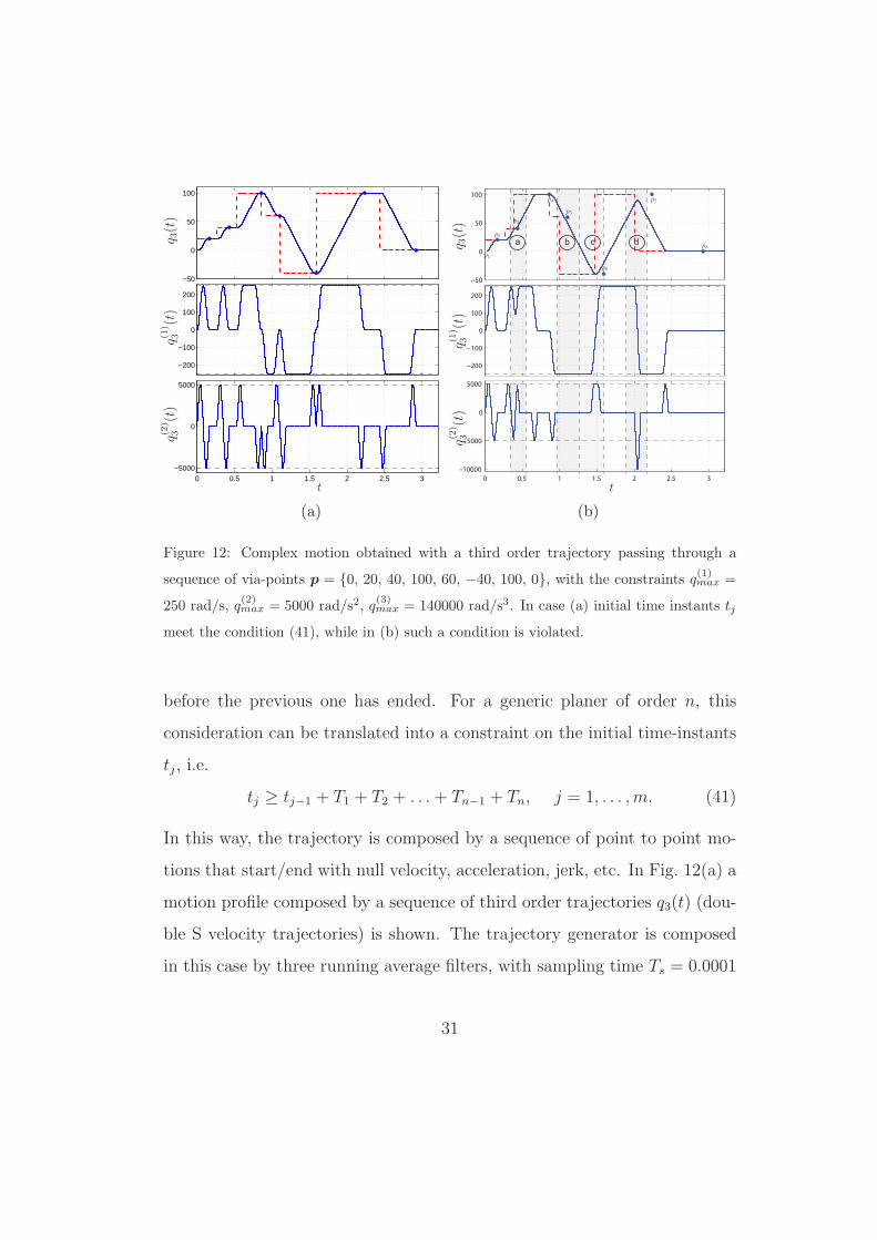
(a) (b)

Figure 12: Complex motion obtained with a third order trajectory passing through a

sequence of via-points p = {0, 20, 40, 100, 60, −40, 100, 0}, with the constraints q(1)max =

250 rad/s, q(2)max = 5000 rad/s2, q

(3)max = 140000 rad/s3. In case (a) initial time instants tj

meet the condition (41), while in (b) such a condition is violated.

before the previous one has ended. For a generic planer of order n, this

consideration can be translated into a constraint on the initial time-instants

tj, i.e.

tj ≥ tj−1 + T1 + T2 + . . .+ Tn−1 + Tn, j = 1, . . . ,m. (41)

In this way, the trajectory is composed by a sequence of point to point mo-

tions that start/end with null velocity, acceleration, jerk, etc. In Fig. 12(a) a

motion profile composed by a sequence of third order trajectories q3(t) (dou-

ble S velocity trajectories) is shown. The trajectory generator is composed

in this case by three running average filters, with sampling time Ts = 0.0001

31

s, defined by the time constants

T1,j =|hj|q(1)max

=|hj|15

s

T2 =q(1)max

q(2)max

= 0.05 s → N2 =0.05

0.0001= 500

T3 =q(2)max

q(3)max

= 0.035 s → N3 =0.035

0.0001= 350

where hj = pj − pj−1, j = 1, . . . ,m represents the displacement of the j-th

tract. Note that the limit values of velocity, acceleration, jerk, are generally

constant and therefore N2 and N3 are the same for all tracts and are fixed

before the motion starts. Conversely, in order to guarantee a constant ve-

locity with different displacements hj, it is necessary to change online the

structure of the first FIR filter of the trajectory planner. In particular, it is

needed to adapt the number of taps of the filter to the desired displacement

value hj, according to the formula N1,j = round(

|hj |

Ts·q(1)max

)

. Obviously, this

operation must be performed whenever the input signal defining the final

position changes (and therefore a new displacement hj is required) and it

must guarantee the continuity of the trajectory and of its derivatives up to

the order n − 1. Since a new via-point is provided only when the previous

one has been reached, when the input changes all the FIR filters (and in par-

ticular the first one) are in a steady-state condition. For the first filter fed

with constant signals, this means that both the output and all the internal

states are equal to the input value. As a consequence, when additional taps

are added to M1(z), in order to keep the output unchanged, it is necessary to

set the values of the new internal states equal to those of the existing states.

When some taps are eliminated, the values of the remaining internal states

32

are not modified.

As above mentioned, the trajectory planned with the proposed generator is

composed by rest to rest motion segments between the via-points and it is not

possible to specify desired values of velocity, acceleration, jerk, etc. different

from zero at these points. However, it is worth noticing that by modifying

(online) the staircase function p(t), the output trajectory does not stop at the

via-points. In Fig. 12(b) different situations that may occur are illustrated.

In cases (a) and (b) the required displacements of two consecutive tracts have

the same sign while in (c) and (d) they are opposite. In particular, in the

tract denoted by (a), the level corresponding to the via-point p4 is provided

before p3 is reached. As a consequence the trajectory crosses p3 without

stopping on it. Note that the velocity firstly decreases and then increases

without becoming zero. In the segment (b), the point p6 is given before the

trajectory starts decelerating. In this manner, the velocity remains constant

at the maximum value. In the segment (c), the input function p(t) is modi-

fied when the acceleration of the previous tract starts decreasing, that is at

time Ttot−T3 being Ttot the total duration of the motion law between p5 and

p6. In this way the deceleration of the former segment and the acceleration

of the latter one, that have the same sign, are superimposed but the two

contributions are compensated each other and the acceleration profile of the

resulting trajectory does not overcome the limit value. A different situation

arises in case (d), where the next via-point p7 is provided (and therefore the

trajectory segment between p6 and p7 begins) before the acceleration of the

previous tract starts decreasing. As a consequence, the deceleration and the

acceleration of the two segments, that also in this case have the same sign,

33

are superimposed and lead to a total acceleration that reaches a peak value

twice the desired bound.

From this analysis, it comes out that the condition (41), that guarantees

that all the segments composing the trajectory are point to point movements

with initial and final derivatives null, is too conservative with respect to the

problem of the compliance with the limits of velocity, acceleration, jerk, etc.

As a matter of fact, only when two consecutive tracts are obtained for dis-

placements with opposite signs the bounds are violated if a new reference

input is provided (more than T3 seconds) before the end of the former seg-

ment. In this case, it is convenient to wait that the trajectory stops at a

given via-point before providing the next reference point. Conversely, if the

next via-point requires a movement in the same direction of the current tra-

jectory, it can be given to the chain of filters at any time. Clearly, in order

to allows a “smooth” modification of the first FIR filter according to the

desired displacement, it is necessary to wait at least T1 seconds from the last

via-point.

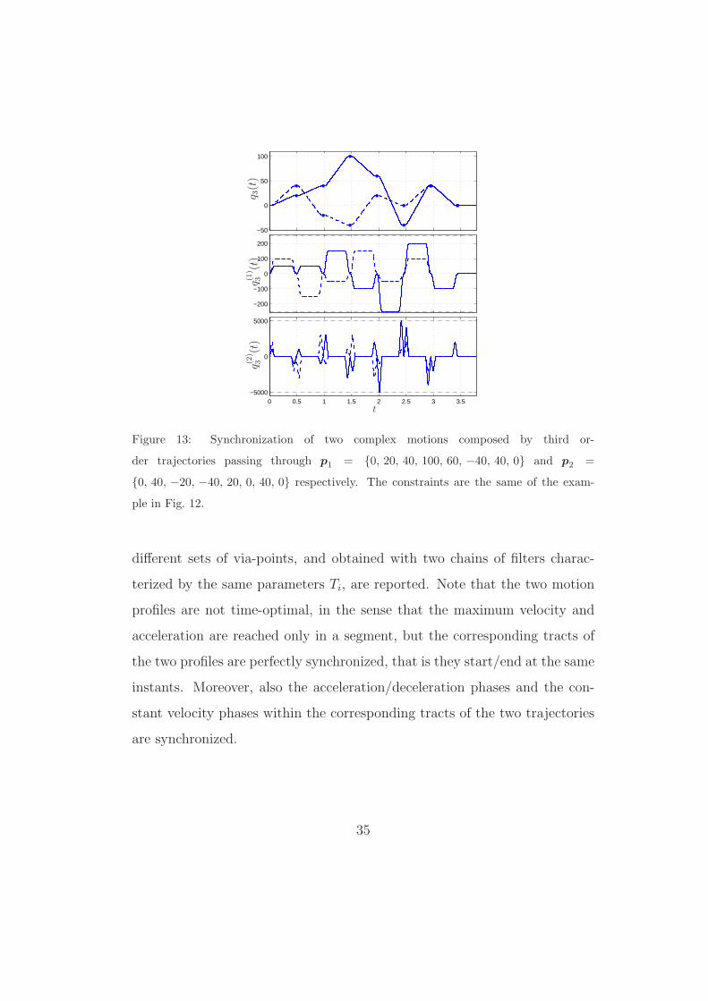
Another possible design strategy for the trajectory planner consists in

assuming a constant value for N1. For instance, if the required displacement

hj are known in advance, one may choose

T1 =maxj(|hj|)

q(1)max

→ N1 = round

(

T1

Ts

)

in order to guarantee that the maximum velocity is never exceeded. In this

way the duration of the trajectory is constant, whatever the displacement hj

may be. This property can be exploited to synchronize the motions among

different axes, as shown in Fig. 13 where the trajectories passing through two

34

0 0.5 1 1.5 2 2.5 3 3.5−5000

0

5000

−200

−100

0

100

200

−50

0

50

100

q 3(t)

q(1)

3(t)

q(2)

3(t)

t

Figure 13: Synchronization of two complex motions composed by third or-

der trajectories passing through p1 = {0, 20, 40, 100, 60, −40, 40, 0} and p2 =

{0, 40, −20, −40, 20, 0, 40, 0} respectively. The constraints are the same of the exam-

ple in Fig. 12.

different sets of via-points, and obtained with two chains of filters charac-

terized by the same parameters Ti, are reported. Note that the two motion

profiles are not time-optimal, in the sense that the maximum velocity and

acceleration are reached only in a segment, but the corresponding tracts of

the two profiles are perfectly synchronized, that is they start/end at the same

instants. Moreover, also the acceleration/deceleration phases and the con-

stant velocity phases within the corresponding tracts of the two trajectories

are synchronized.

35

4.2. Multi-segment trajectories with frequency specifications

In the previous example the parameters of the trajectory generator are

obtained on the basis of constraints (velocity, acceleration, jerk) expressed

in the time-domain. On the other hand, as already mentioned, it is also

possible to take into account frequency constraints, that may arise because

of critical frequencies of the plant that tracks this motion profile. There-

fore, it is possible to combine the advantages of time-optimal multi-segment

trajectories with those of the approaches that filter the input trajectories to

properly shape their spectrum, see Singer et al. (1999) for a comprehensive

overview on this argument.

Let us consider the standard motion system shown in Fig. 14, composed by

two inertias with an elastic transmission lightly damped (Lambrechts et al.,

2005; Barre et al., 2005; Meckl and Arestides, 1998), whose model (from the

motor position qm to the load position ql) can be described by the transfer

function

Gml(s) =Ql(s)

Qm(s)=

2δωns+ ω2n

s2 + 2δωns+ ω2n

(42)

τle

Jl

ql

τm

Jm

qm

kt

bt

Figure 14: Lumped constant model of a motion system with elastic transmission.

36

Parameter Symbol Value Unit

Motor inertia Jm 0.72× 10−5 kgm2

Load inertia Jl 0.23× 10−5 kgm2

Spring stiffness kt 0.156 Nm

Internal damping bt 1.0× 10−5 Nms

Table 1: Motion system parameters.

with

ωn =

√

ktJl, δ =

bt

2√ktJl

.

The parameters of the system, reported in Tab. 1, are derived from Lam-

brechts et al. (2005), as well as the trajectory constraints (q(1)max = 250 rad/s,

q(2)max = 5000 rad/s2, q

(3)max = 5 × 105 rad/s3). The resonant frequency of the

system results ωr ≈ ωn = 260.43 rad/s, while δ = 0.0083.

By supposing that an ideal control system imposes to the motor (Jm) the

desired motion profile, that is qm(t) = qref (t), being qref (t) a trajectory ob-

tained with the generator proposed in previous sections, it is possible to

analyze the effects of a particular choice of the trajectory parameters on the

dynamic behavior of the plant and in particular on the tracking error, de-

fined as ε(t) = qref (t) − ql(t) = qm(t) − ql(t). Obviously, the choice of the

parameters of the filter is critical only when the spectral components of the

trajectory are appreciable in the neighborhood of the eigenfrequency of the

plant. If this occurs, a design of the trajectory that neglects the dynamic

characteristics of the plant may lead to large tracking errors during the mo-

tion, and to residual oscillations when the motion stops. For instance, the

response of Gml(s) to a trapezoidal velocity trajectory obtained by assuming

37

0 0.02 0.04 0.06 0.08 0.1 0.12−1

−0.5

0

0.5

10

5

10

15

20

25q 2(t)

ε(t)

t0 100 200 300 400 500 600 700

0

100

200

300

400

500

600

700

800

900

ω

V(ω

)

(a) (b)

Figure 15: Response of the elastic system Gml(s) to a trapezoidal velocity trajectory

obtained with T1 = 0.064 s and T2 = 0.032 s: tracking error (a) and frequency spectrum

of the acceleration (b).

T1 = 0.064 s and T2 = 0.032 s (Ttot = 0.096 s) is shown in Fig. 15(a) along

with the error ε(t). Note the considerable value of the error at the end of

motion, in particular if compared with the error obtained by applying to the

system the trapezoidal velocity trajectory of Fig. 16, characterized by the

same total duration Ttot = 0.096 s, but obtained with T1 = 3T0 and T2 = T0

(being T0 = 2πωr

= 0.0242 s the natural period of Gml(s)). By analyzing the

spectral contents of the two trajectories, and in particular of the acceleration

profiles, it is possible to explain such results. The dynamic relation between

the reference trajectory qref (t) and the tracking error ε, obtained from (42)

after simple algebraic manipulations, is given by

E(s)

Qref (s)=

s2

s2 + 2δωns+ ω2n

(43)

38

0 0.02 0.04 0.06 0.08 0.1 0.12−1

−0.5

0

0.5

10

5

10

15

20

25q 2(t)

ε(t)

t0 100 200 300 400 500 600 700

0

100

200

300

400

500

600

700

800

900

ω

V(ω

)

(a) (b)

Figure 16: Response of the elastic system Gml(s) to a trapezoidal velocity trajectory

obtained with T1 = 3T0 and T2 = T0: tracking error (a) and frequency spectrum of the

acceleration (b).

where E(s) = L{ε(t)} and Qref (s) = L{qref (t)}. Note that (43) can be

rewritten as

E(s)

Q(2)ref (s)

=E(s)

s2 Qref (s)=

1

s2 + 2δωns+ ω2n

= Gε(s)

that is ε can be obtained by applying the second derivative of the reference

signal qref (t) = qn(t), i.e. the acceleration profile q(2)n (t), to the second order

system Gε(s) characterized by a natural frequency ωn and a damping factor

δ. For this reason in Fig. 15(b) and Fig. 16(b) the spectrum |Q(2)n (jω)| of

the acceleration profile, hereafter denoted with V (ω), is compared with the

magnitude of the frequency response of Gε(s) (properly scaled for the sake

of clarity).

From the considerations of Sec.2.3, it follows that the parameters

T1 = 3T0 ⇔ ω1 =ωr

3

39

and

T2 = T0 ⇔ ω2 = ωr

lead to |M1(jωr)| = 0, and |M2(jωr)| = 0, and therefore they introduce in

V (ω) a zero of multiplicity two for ω = ωr. This implies that not only

V (ωr) = 0,

but alsodV (ω)

dω |ω=ωr

= 0

and, as a consequence, in the neighborhood of the resonant frequency ωr the

slope of V (ω) is small and the function remains limited in a broad range of

frequencies.

The use of double S velocity trajectories (with limited jerk) can further im-

prove the result in terms of magnitude of the tracking error as highlighted

in a number of works, see (Lambrechts et al., 2005; Barre et al., 2005; Meckl

and Arestides, 1998). But also in this case the choice of the filter/trajectory

parameters has a strong influence on the system output, as shown in Fig. 17

and Fig. 18 where two double S velocity trajectories of the same duration

are compared. In particular, a choice of the time constants T1, T2, T3 that

does not take into account the presence of a resonant peak into the system3

does not produce any improvement in the tracking performances with re-

3Note that the values

T1 =5

2T0 ⇔ ω1 =

2

5ωr

T2 = T3 =3

4T0 ⇔ ω2 = ω3 =

4

3ωr

do not guarantee that V (ωr) = 0, as shown in Fig. 17(b).

40

0 0.02 0.04 0.06 0.08 0.1 0.12−1

−0.5

0

0.5

10

5

10

15

20

25q 3(t)

ε(t)

t0 100 200 300 400 500 600 700

0

100

200

300

400

500

600

700

800

900

ω

V(ω

)

(a) (b)

Figure 17: Response of the elastic system Gml to a double S velocity trajectory obtained

with T1 = 5/2T0, T2 = 3/4T0 and T3 = 3/4T0: tracking error (a) and frequency spectrum

of the acceleration (b).

spect to lower order trajectories such as trapezoidal velocity trajectories, see

Fig. 17. On the contrary, by assuming the parameters T1 = 2T0, T2 = T0

and T3 = T0 the spectrum of the trajectory V (ωr) has a zero of multiplicity

three for ω = ωr, and therefore

V (ωr) =dV (ω)

dω |ω=ωr

=d2V (ω)

dω2 |ω=ωr

= 0.

From a practical point of view, this means that the values of the function

V (ω) in the neighborhood of the resonant frequency are smaller than those

of the trapezoidal velocity trajectory of Fig. 16, whose parameters Ti are

obtained with similar considerations. As a consequence, the tracking error

of the plant is reduced. In particular for the trapezoidal velocity trajectory

the maximum value of the error is max |εtr| = 0.3395, while for the double S

velocity trajectory max |ε2S| = 0.2536, with a reduction ∆|ε| ≈ −25%.

41

0 0.02 0.04 0.06 0.08 0.1 0.12−1

−0.5

0

0.5

10

5

10

15

20

25q 3(t)

ε(t)

t0 100 200 300 400 500 600 700

0

100

200

300

400

500

600

700

800

900

ω

V(ω

)

(a) (b)

Figure 18: Response of the elastic system Gml to a double S velocity trajectory obtained

with T1 = 2T0, T2 = T0 and T3 = T0: tracking error (a) and frequency spectrum of the

acceleration (b).

4.3. Combining time- and frequency-domain specifications

In the examples discussed so far, only the constraints due to the dynamic

behavior of the plant have been considered, while the bounds on velocity,

acceleration, etc. have not been taken into account. As a consequence,

the peak values of q(1)(t), q(2)(t), etc. depend on the choice of the pa-

rameters Ti. For instance, in the case of the double S velocity trajectory

of Fig. 18(a), the values of such parameters lead to q(1)max = |h|/T1 = 276

rad/s (being the displacement h = 20 rad), q(2)max = q

(1)max/T2 = 11454 rad/s2,

q(3)max = q

(2)max/T3 = 474750 rad/s3. However, the interpretation of multi-

segment trajectories as a bank of filters allows to combine time and frequency

constraints. This feature must be profitably exploited in all those cases in

which the actuation system imposes some physical limits and the load intro-

duces undesired dynamical modes.

For instance, with reference to the plant Gml(s), if the actuation system

42

0 0.05 0.1 0.15 0.2−0.1

−0.05

0

0.05

0.10

5

10

15

20

25q 3(t)

ε(t)

t0 100 200 300 400 500 600 700

0

50

100

150

200

250

300

350

400

450

ω

V(ω

)

(a) (b)

Figure 19: Response of the elastic system Gml(s) to a double S velocity trajectory obtained

with T1 = |h|/q(1)max, T2 = q(1)max/q

(2)max and T3 = T1 − T2: tracking error (a) and frequency

spectrum of the acceleration (b).

is capable of providing a maximum speed q(1)max and a maximum acceleration

q(2)max, a minimum time double S velocity trajectory can be obtained by as-

suming T1 = h/q(1)max and T2 = q

(1)max/q

(2)max, while the parameter T3 can be set

to the minimum value compliant with constraints (19), that is T3 = T1 − T2.

However, although the error is about one order smaller than the error of the

trajectories of Fig. 16 and Fig. 18 obtained by tacking into account only the

dynamical model of the plant4, it exhibits some oscillations when the tra-

jectory stops, as highlighted in Fig. 19(a). In order to reduce these residual

vibrations one can set the free parameters T3 to T0 in order to make V (ω)

null for ω = ωr, see Fig. 20. In this way, the resonant mode of the plant

4This is due to the total duration of the trajectory obtained with the time constraints,

Ttot = 0.16 s, which is pretty higher than the duration of the other trajectories, Ttot =

0.0965 s. For this reason the magnitude of spectral components at high frequencies is

considerably reduced.

43

0 0.05 0.1 0.15 0.2−0.1

−0.05

0

0.05

0.10

5

10

15

20

25q 3(t)

ε(t)

t0 100 200 300 400 500 600 700

0

50

100

150

200

250

300

350

400

450

ω

V(ω

)

(a) (b)

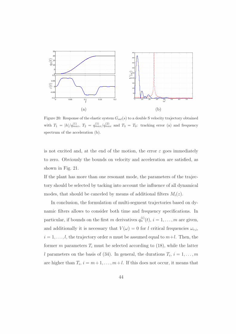
Figure 20: Response of the elastic system Gml(s) to a double S velocity trajectory obtained

with T1 = |h|/q(1)max, T2 = q(1)max/q

(2)max and T3 = T0: tracking error (a) and frequency

spectrum of the acceleration (b).

is not excited and, at the end of the motion, the error ε goes immediately

to zero. Obviously the bounds on velocity and acceleration are satisfied, as

shown in Fig. 21.

If the plant has more than one resonant mode, the parameters of the trajec-

tory should be selected by tacking into account the influence of all dynamical

modes, that should be canceled by means of additional filters Mi(z).

In conclusion, the formulation of multi-segment trajectories based on dy-

namic filters allows to consider both time and frequency specifications. In

particular, if bounds on the first m derivatives q(i)n (t), i = 1, . . . ,m are given,

and additionally it is necessary that V (ω) = 0 for l critical frequencies ωr,i,

i = 1, . . . , l, the trajectory order n must be assumed equal tom+l. Then, the

former m parameters Ti must be selected according to (18), while the latter

l parameters on the basis of (34). In general, the durations Ti, i = 1, . . . ,m

are higher than Ti, i = m+1, . . . ,m+ l. If this does not occur, it means that

44

0 0.02 0.04 0.06 0.08 0.1 0.12 0.14 0.16−6000

−4000

−2000

0

2000

4000

6000

0

100

200

3000

5

10

15

20

25

q 3(t)

q(1)

3(t)

q(2)

3(t)

t

Figure 21: Profiles of position, velocity and acceleration of the trajectory considered in

Fig. 20.

the constraints due to dynamical reasons guarantee also the compliance with

the limits on velocity, acceleration, jerk, etc. In this case, one can neglect

such bounds, that are met in any case because of the frequency constraints,

and reduce the order of the trajectory.

5. Conclusions

In this paper, the equivalence between multi-segment trajectories and the

output of chains of moving average filters has been demonstrated. This result

has been the starting point for a generalization of this type of trajectories,

that are usually limited to second order (trapezoidal velocity trajectories)

or third order (double S velocity trajectories), to a generic order n. In this

case the trajectory generator is composed by a cascade of n FIR filters to be

fed with a step function signal which defines the desired final position. This

45

implies a low complexity and an high efficiency of the trajectory planner,

also for large values of n. Moreover, its modular structure, composed by

linear filters, provides an immediate characterization of the output trajectory

from a frequency point of view. This type of analysis allows to define the

parameters of the trajectory from frequency considerations and not only on

the basis of classical constraints on maximum velocity, acceleration, jerk,

etc. Simulative examples help to explain the use of filters for multi-point

trajectories planning and the techniques for the design of filters parameters

considering both frequency and time specifications.

References

Barre, P.-J., Bearee, R., Borne, P., Dumetz, E., 2005. Influence of a jerk

controlled movement law on the vibratory behaviour of high-dynamics sys-

tems. Journal of Intelligent and Robotic Systems 42, 275–293.

Biagiotti, L., Melchiorri, C., 2008. Trajectory Planning for Automatic Ma-

chines and Robots. Springer Berlin Heidelberg.

Bonfe, M., Secchi, C., 2010. Online smooth trajectory planning for mobile

robots by means of nonlinear filters. In: Intelligent Robots and Systems

(IROS), 2010 IEEE/RSJ International Conference on. pp. 4299 –4304.

Fortgang, J., Singhose, W., Mrquez, J. d. J., 2005. Command shaping for

micro-mills and cnc controllers. In: Proc. American Control Conference.

Franklin, G. F., Powell, J. D., Workman, M. L., 1998. Digital Control of

Dynamic Systems, 3rd Edition. Ellis-Kagle Press.

46

Gerelli, O., Guarino Lo Bianco, C., 2008. Real-time path-tracking control

of robotic manipulators with bounded torques and torque-derivatives. In:

IROS. pp. 532–537.

Gerelli, O., Guarino Lo Bianco, C., 2009. Nonlinear variable structure filter

for the online trajectory scaling. Industrial Electronics, IEEE Transactions

on 56 (10), 3921 –3930.

Hong, K.-T., Hong, 2004. Input shaping and vsc of container cranes. In: Proc.

IEEE International Conference on Control Applications. pp. 1570–1575.

Jeon, J. W., Ha, Y. Y., 2000. A generalized approach for the acceleration and

deceleration of industrial robots and cnc machine tools. IEEE Transactions

on Industrial Electronics 74, no 1, 133–139.

Kim, D.-I., Jeon, J. W., Kim, S., 1994. Software acceleration/deceleration

methods for industrial robots and cnc machine tools. Mechatronics 4 (1),

37–53.

Lambrechts, P., Boerlage, M., Steinbuch, M., 2005. Trajectory planning and

feedforward design for electromechanical motion systems. Control Engi-

neering Practice 13, 145–157.

Magee, D., Book, W., 1998. Optimal filtering to minimize the elastic behav-

ior in serial link manipulators. In: American Control Conference, 1998.

Proceedings of the 1998. Vol. 5. Philadelphia, PA , USA, pp. 2637 – 2642.

Meckl, P., Arestides, P., 1998. Optimized s-curve motion profiles for mini-

mum residual vibration. In: Proceedings of the American Control Confer-

ence. Philadelphia, Pennsylvania, pp. 2627–2631.

47

Nozawa, R., Kawamura, H., Sasaki, T., 1985. Acceleration/decelaration cir-

cuit.

Olabi, A., Bearee, R., Gibaru, O., Damak, M., 2010. Feedrate planning for

machining with industrial six-axis robots. Control Engineering Practice

18 (5), 471–482.

Singer, N., Singhose, W., Seering, W., 1999. Comparison of filtering methods

for reducing residual vibration. European Journal of Control 5, 208–218.

Singer, N. C., Seering, W. P., 1990. Preshaping command inputs to reduce

system vibration. ASME Journal of Dynamic Systems, Measurement, and

Control 112, 76–82.

Singhose, W., 2009. Command shaping for flexible systems: A review of the

first 50 years. International Journal Of Precision Engineering And Manu-

facturing 10 (4), 153–168.

Tuttle, T., Seering, W., 1994. A zero-placement technique for designing

shaped inputs to suppress multiple-mode vibration. In: American Con-

trol Conference, 1994. Vol. 3. pp. 2533 – 2537.

Zanasi, R., Bianco, C. G. L., Tonielli, A., 2000. Nonlinear filter for the gen-

eration of smooth trajectories. Automatica 36, 439–448.

Zanasi, R., Morselli, R., 2003. Discrete minimum time tracking problem for

a chain of three integrators with bounded input. Automatica 39 (9), 1643–

1649.

48

Zheng, C., Su, Y., Muller, P., 2009. Simple online smooth trajectory gener-

ations for industrial systems. Mechatronics 19, 571–576.

49