Financial Frictions, Investment, and Tobin’s q

Dan Cao

Georgetown University

Guido Lorenzoni

Northwestern University

Karl Walentin

Sveriges Riksbank

November 21, 2016

Abstract

We develop a model of investment with financial constraints and use it to

investigate the relation between investment and Tobin’s q. A firm is financed

partly by insiders, who control its assets, and partly by outside investors.

When insiders’ wealth is scarce, they earn a rate of return higher than the

market rate of return and thus the firm’s value includes a quasi-rent on in-

vested capital. This implies that two forces drive q: changes in the value of

invested capital and changes in the value of the insiders’ future rents per unit

of capital. This weakens the correlation between q and investment, relative

to the frictionless benchmark. We present a calibrated version of the model,

which, due to this effect, can generate more realistic correlations between in-

vestment, q, and cash flow.

Keywords: Financial constraints, optimal financial contracts, investment, To-

bin’s q, limited enforcement.

JEL codes: E22, E30, E44, G30.

1 Introduction

Dynamic models of the firm imply that investment decisions and the value of thefirm should both respond to expectations about future profitability of capital. Inmodels with constant returns to scale and convex adjustment costs these relationsare especially clean, as investment and the firm’s value respond exactly in thesame way to new information about future profitability. This is the main predic-tion of Tobin’s q theory, which implies that current investment moves one-for-onewith q, the ratio of the firm’s financial market value to its capital stock. This pre-diction, however, is typically rejected in the data, where investment appears tocorrelate more strongly with current cash flow than with q.

In this paper, we investigate the relation between investment, q, and cash flowin a model with financial frictions. The presence of financial frictions introducesquasi-rents in the market valuation of the firm. These quasi-rents break the one-to-one link between investment and q. We study how the presence of these quasi-rents affects the statistical correlations between investment, q, and cash flow, andask whether a model with financial frictions can match the correlations in the data.

Our main conclusion is that the presence of financial frictions can bring themodel closer to the data, but that the model’s implications depend crucially onthe shock structure. The crucial observation is that in a model with financial fric-tions it is still true that investment and q respond to future profitability, but thetwo variables now respond differently to information at different horizons. In-vestment is particularly sensitive to current profitability, which determines cur-rent internal financing, and to near-term financial profitability, which determinescollateral values. On the other hand, q is relatively more sensitive to profitabilityfarther in the future, which will determine future growth and thus the size of fu-ture quasi-rents. Therefore, to break the link between investment and q, we needthe presence of both short-lived shocks—which tend to move investment moreand have relatively smaller effects on q—and long-lived shocks—which do theopposite.

To develop these points, we build a stochastic model of investment subject to

1

limited enforcement, with fully state-contingent claims. We show that our limitedenforcement constraint is equivalent to a state-contingent collateral constraint, soour model is essentially a stochastic version of Kiyotaki and Moore (1997) withadjustment costs and state-contingent claims.1 We show that the model leads toa wedge between average q—which correspond to the q measured from financialmarket values—and marginal q—which captures the marginal incentive to investand is related one-to-one to investment.2 We then analyze two versions of themodel and look at their implications for an investment regression in which theinvestment rate is regressed on average q and cash flow.

First, we focus on a version of the model with no adjustment costs, which,under some simplifying assumptions, can be linearized and studied analytically.We consider three different shock structures. In a case with a single persistentshock, the model has indeterminate predictions regarding investment regressioncoefficients. This simply follow because in this case q and cash flow are perfectlycollinear. In a case with two shocks—a temporary shock and a persistent shock—the one-to-one relation between q and investment breaks down because invest-ment is driven by productivity in periods t and t+ 1 while q responds to all futurevalues of productivity. Finally, we consider a case with “news shocks”, that is,we allow agents to observe J periods in advance the realization of productivityshocks. In this case, we show that increasing the length of the horizon J reducesthe coefficient on q and increases the coefficient on cash flow in investment re-gressions. This is due again to the differential responses of investment and q toinformation on productivity at different horizons.

The model with no adjustment costs, while analytically tractable, is quantita-tively unappealing, as it tends to produce too much short-run volatility and toolittle persistence in investment. Therefore, for a more quantitative evaluation ofthe model we introduce adjustment costs. We calibrate the model to data moments

1Related recent stochastic models that combine state-contingent claims with some form of col-lateral constraint include He and Krishnamurthy (2013), Rampini and Viswanathan (2013) andDi Tella (2016).

2The terminology goes back to Hayashi (1982), who shows that the two are equivalent in acanonical model with convex adjustment costs.

2

from Compustat and analyze its implications both in terms of impulse responsesand in terms of investment regressions. Our baseline calibration is based on thetwo shocks structure, with temporary and persistent shocks. In this calibrationwe show that q responds relatively more strongly to the persistent shock whileinvestment responds relatively more strongly to the transitory shock, in line withthe intuition from the no-adjustment-cost case. This leads to investment regres-sions with a smaller coefficient on q and a larger coefficient on cash flow, relativeto a model with no financial frictions, thus bringing us closer to empirical coeffi-cients. However, the q coefficient is still larger than in the data and the cash flowcoefficient is smaller than in the data. When adding the possibility of news shocks,the disconnect between q and investment increases, leading to further reductionsin the q coefficient and increases in the cash flow coefficient.

Fazzari et al. (1988) started a large empirical literature that explores the rela-tion between investment and q using firm-level data. The typical finding in thisliterature is a small coefficient on q and a positive and significant coefficient oncash flow.3 Fazzari et al. (1988), Gilchrist and Himmelberg (1995) and most ofthe subsequent literature interpret these findings as a symptom of financial fric-tions at work. More recent work by Gomes (2001) and Cooper and Ejarque (2003)questions this interpretation. The approach taken in these two papers is to lookat the statistical implications of simulated data generated by a model to under-stand the empirical correlations between investment, q and cash flow.4 In theirsimulated economies with financial frictions q still explains most of the variabil-ity in investment, and cash flow does not provide additional explanatory power.In this paper, we take a similar approach but reach different conclusions. This isdue to two main differences. First, Gomes (2001) and Cooper and Ejarque (2003)model financial frictions by introducing a transaction cost which is a function ofthe flow of outside finance issued each period, while we introduce a contractualimperfection that imposes an upper bound on the stock of outside liabilities as afraction of total assets. Our approach adds a state variable to the problem, namely

3See Hubbard (1998) for a survey.4An approach that goes back to Sargent (1980).

3

the stock of existing liabilities of the firm as a fraction of assets, thus generatingslower dynamics in the gap between internal funds and the desired level of in-vestment. Second, we explore a variety of shock structures, which, as we arguebelow, play an important role in our results.

A related strand of recent literature has focused on violations of q theory com-ing from decreasing returns or market power, leaving aside financial frictions.5

We see our effort as complementary to this literature, since both financial frictionsand decreasing returns determine the presence of future rents embedded in thevalue of the firm. Also in that literature the shock structure plays an importantrole in the results. For example, Eberly et al. (2008) show that it is easier to obtainrealistic implications for investment regressions by assuming a Markov processin which the distribution from which persistent productivity shocks are drawnswitches occasionally between two regimes. Abel and Eberly (2011) also showthat in models with decreasing returns it is possible to obtain interesting dynam-ics in q with no adjustment costs, similarly to what we do in Section 3 in a modelwith constant returns to scale and financial constraints.

The simplest shock that breaks the link between q and investment in modelswith financial constraints is a purely temporary shock to cash flow, which does notaffect capital’s future productivity. Absent financial frictions this shock shouldhave no effect on current investment. This idea is the basis of a strand of em-pirical literature that tests for financial constraints by identifying some source ofpurely temporary shocks to cash flow. This is the approach taken by Blanchardet al. (1994) and Rauh (2006), which provide reliable evidence of the presence offinancial constraints. Our paper builds on a similar intuition, by showing that ingeneral shocks affecting profitability at different horizons have differential effectson q and investment and asks whether, given a realistic mix of shocks, a modelwith financial frictions can produce the unconditional correlations observed inthe data.

In this paper we use the simplest possible model with the features we need:

5See Schiantarelli and Georgoutsos (1990) Alti (2003), Moyen (2004), Eberly et al. (2008), Abeland Eberly (2011),Abel and Eberly (2012), .

4

an occasionally binding financial constraint; a dynamic, stochastic structure; ad-justment costs that can produce realistic investment dynamics. There is a growingliterature that builds richer models that are geared more directly to estimation.In particular, Hennessy and Whited (2007) build a rich structural model of firms’investment with financial frictions, which is estimated by simulated method ofmoments. They find that the financial constraint plays an important role in ex-plaining observed firms’ behavior. In their model, due to the complexity of theestimation task, the financial friction is introduced in a reduced form manner, byassuming transaction costs associated to the issuance of new equity or debt, as inGomes (2001) or Cooper and Ejarque (2003).6 We see our effort as complementary,as we have a more stylized model, but with financial constraints coming from anexplicitly modeled contractual imperfection.

A growing number of papers uses recursive methods to characterize optimaldynamic financial contracts in environments with different forms of contractualfrictions (Atkeson and Cole (2005), Clementi and Hopenhayn (2006), DeMarzoand Sannikov (2006), DeMarzo et al. (2012)). The limited enforcement friction inthis paper makes it closer to the models in Albuquerque and Hopenhayn (2004)and Cooley et al. (2004). Within this literature Biais et al. (2007) look more closelyat the implications of the theory for asset pricing. In particular, they find a setof securities that implements the optimal contract and then study the stochasticbehavior of the prices of these securities. Here, our objective is to examine themodel’s implication for q theory, therefore we simply focus on the total value ofthe firm, which includes the value of all the claims held by insiders and outsiders.

In Section 2 we present the model. In Section 3, we study the case of no ad-justment costs, deriving analytical results. In Section 4, we study the model withadjustment costs, relying on numerical simulations.

6The difference in results, relative to these papers, appears due to the fact that Hennessy andWhited (2007) also match the behavior of a number of financial variables.

5

2 The Model

Consider an infinite horizon economy, in discrete time, populated by a continuumof entrepreneurs who invest in physical capital and raise funds from risk neutralinvestors.

The entrepreneurs’ technology is linear: Kit units of capital, installed at timet − 1 by entrepreneur i, yield profits AitKit at time t. We can think of the linearprofit function AitKit as coming from a constant returns to scale production func-tion in capital and other variable inputs which can be costlessly adjusted. There-fore, changes in Ait capture both changes in technology and changes in input andoutput prices. For brevity, we just call Ait “productivity”. Productivity is a func-tion of the state sit, Ait = A (sit), where sit is a Markov process with a finite statespace S and transition probability π (sit|sit−1). There are no aggregate shocks, sothe cross sectional distribution of sit across entrepreneurs is constant.

Investment is subject to convex adjustment costs. The cost of changing theinstalled capital stock from Kit to Kit+1 is G (Kit+1, Kit) units of consumption goodsat date t. The function G includes both the cost of purchasing capital goods andthe installation cost. We assume G is increasing and convex in its first argument,decreasing in the second argument, and displays constant returns to scale. Fornumerical results, we use the quadratic functional form

G (Kit+1, Kit) = Kit+1 − (1− δ)Kit +ξ

2(Kit+1 − Kit)

2

Kit. (1)

All agents in the model are risk neutral. The entrepreneurs’ discount factoris β and the investors’ discount factor is β, with β > β. We assume investorshave a large enough endowment of the consumption good each period so that theequilibrium interest rate is 1 + r = 1/β. Each period an entrepreneur retires withprobability γ and is replaced by a new entrepreneur with an endowment of 1 unitof capital. When an entrepreneur retires, productivity Ait is zero from next periodon. The retirement shock is embedded in the process sit by assuming that there isan absorbing state sr with A(sr) = 0 and the probability of transitioning to sr from

6

any other state is γ.Each period, entrepreneur i can issue one-period state contingent liabilities,

subject to limited enforcement. The entrepreneur controls the firm’s capital Kit

and, at the beginning of each period, can default on his liabilities and divert afraction 1− θ of the firm’s capital. If he does so, he re-enters the financial mar-ket as a new entrepreneur, with capital (1− θ)Kit and no liabilities. That is, thepunishment for a defaulting entrepreneur is the loss of a fraction θ of the firm’sassets.

2.1 Optimal investment

We formulate the optimization problem of the individual entrepreneur in recur-sive form, dropping the subscripts i and t. Let V (K, B, s) be the expected utility ofan entrepreneur in state s, who enters the period with capital stock K and currentliabilities B. For now, we simply assume that the problem’s parameters are suchthat the entrepreneur’s optimization problem is well defined. In the followingsections, we provide conditions that ensure that this is the case.7 The function Vsatisfies the Bellman equation

V (K, B, s) = maxC≥0,K′≥0,{B′(s′)}

C + βE[V(K′, B′

(s′)

, s′)|s]

, (2)

subject to

C + G(K′, K

)≤ A(s)K− B + βE

[B′(s′)|s]

, (3)

V(K′, B′

(s′)

, s′)≥ V

((1− θ)K′, 0, s′

), ∀s′, (4)

where C is current consumption, K′ is next period’s capital stock , and B′ (s′)are next period’s liabilities contingent on s′. Constraint (3) is the budget con-straint and βE [B′ (s′) |s] are the funds raised by selling the state contingent claims{B′ (s′)} to the investors. Constraint (4) is the enforcement constraint that requires

7In the Online Appendix we provide a general existence result.

7

the continuation value under repayment to be greater than or equal to the contin-uation value under default.

The assumption of constant returns to scale implies that the value functiontakes the form V (K, B, s) = v (b, s)K for some function v, where b = B/K is theratio of current liabilities to the capital stock. We can then rewrite the Bellmanequation as

v (b, s)K = maxC≥0,K′≥0{b′(s′)}

C + βE[v(b′(s′)

, s′)|s]

K′, (5)

subject to

C + G(K′, K

)≤ A(s)K− bK + βE

[b′(s′)|s]

K′, (6)

v(b′(s′)

, s′)≥ (1− θ) v

(0, s′

), ∀s′. (7)

It is easy to show that v is strictly decreasing in b. We can then find state-contingent borrowing limits b(s′) such that the enforcement constraint can bewritten as

b′(s′)≤ b

(s′)

, ∀s′. (8)

So the enforcement constraint is equivalent to a state contingent upper bound onthe ratio of the firm’s liabilities to capital. Relative to existing models with col-lateral constraints, two distinguishing features of our model are that we allow forstate-contingent claims and we derive the state-contingent bounds endogenouslyfrom limited enforcement.8

8Other recent models that allow for state-contingent claims include He and Krishnamurthy(2013) and Rampini and Viswanathan (2013). Cao (2013) develops a general model with an explicitstochastic structure that studies collateral constraints with non-state-contingent debt.

8

2.2 Average and Marginal q

To characterize the solution to the entrepreneur’s problem let us start from thefirst order condition for K′:

λG1(K′, K

)= λβE

[b′|s]+ βE

[v′|s]

, (9)

where λ is the Lagrange multiplier on the budget constraint (6), or the marginalvalue of wealth for the entrepreneur. The expressions E [b′|s] and E [v′|s] areshorthand for E [b′ (s′) |s] and E [v (b′ (s′) , s′) |s]. Optimality for consumption im-plies that λ ≥ 1 and the non-negativity constraint on consumption is binding ifλ > 1.

To interpret condition (9) rewrite it as:

λ =βE [v′|s]

G1 (K′, K)− βE [b′|s]≥ 1. (10)

When the inequality is strict the entrepreneur strictly prefers reducing currentconsumption to invest in new units of capital. If C was positive the entrepreneurcould reduce it and use the additional funds to increase the capital stock. Themarginal cost of an extra unit of capital is G1(K′, K) but the extra unit of capitalincreases collateral and allows the entrepreneur to borrow βE [b′|s] more fromthe consumers. So a unit reduction in consumption leads to a levered increasein capital invested of 1/(G1 − βE [b′|s]). Since capital tomorrow increases futureutility by βE [v′|s], we obtain (10).

Condition (9) can be used to derive our main result on average and marginalq. The value of all the claims on the firm’s future earnings, held by investors andby the entrepreneur at the end of the period, is

βE[B′(s′)|s]+ βE

[V(K′, B′

(s′)

, s′)|s]

.

9

Dividing by total capital invested gives us average q:

qa ≡ βE[b′|s]+ βE

[v′|s]

.

Marginal q, on the other hand, is just the marginal cost of one unit of new capital,qm ≡ G1 (K′, K). We can then rearrange equation (9) and express it in terms of qa

and qm as:

qa = qm +λ− 1

λβE[v′|s]

. (11)

Since λ > 1 if only if the non-negativity constraint on consumption is binding, wehave proved the following result.

Proposition 1. Average q is greater than or equal to marginal q, with strict equality ifand only if the non-negativity constraint on consumption is binding.

The difference between average and marginal q is larger if either the Lagrangemultiplier λ is larger or the future value of entrepreneurial equity E [v′|s] is larger,as we can see from equation (11). As we shall see in the numerical part of thepaper, an increase in indebtedness b increases λ but reduces the future value ofentrepreneurial equity, so in general the relation between b and qa − qm can benon-monotone. There is a cutoff for b such that λ = 1 below the cutoff and λ > 1above the cutoff, so we know the relation is increasing in some region.

The fact that the only Lagrange multiplier appearing in (11) is λ, does notmean that the collateral constraint is not relevant in determining the gap betweenaverage and marginal q. Consider the first order condition for b′

βλ + βvb(b′(s′)

, s′)= µ(s′),

where µ(s′) is the Lagrange multiplier on the enforcement constraint (8) (expressedas a ratio of π(s′|s)K′ for convenience). Using the envelope condition for b to sub-stitute for vb and using time subscripts we can then write

λt =β

βλt+1 +

1β

µt+1. (12)

10

This condition shows that λt is a forward looking variable determined by currentand future values of µt+1. Positive values of this Lagrange multiplier in the futureinduce the entrepreneur to reduce consumption today to increase internal fundsavailable. The forward looking nature of λt will be useful to interpret some of ournumerical results about news shocks.

If β = β, condition (12) implies that if, at some date t, the entrepreneur’s con-sumption is positive and λt = 1, then the non-negativity constraint and the col-lateral constraint can not be binding at any future date. In other words, once theentrepreneur is unconstrained he can never go back to being constrained. This isdue to the assumption of complete state contingent markets. Assuming β < β

ensures that entrepreneurs can alternate between positive and zero consumption.We conclude this section by introducing some asset pricing relations that will

be used to characterize the equilibrium. We use the notation G1,t and G2,t as short-hand for G1 (Kt+1, Kt) and G2 (Kt+1, Kt).

Proposition 2. The following conditions hold in equilibrium

λt = βEt

[λt+1

At+1 − G2,t+1 − bt+1

G1,t − βEtbt+1

], (13)

andβEt

[At+1 − G2,t+1

G1,t

]≥ 1 ≥ Et

[βλt+1

λt

At+1 − G2,t+1

G1,t

]. (14)

The last two conditions hold with strict inequality if the collateral constraint is bindingwith positive probability.

Notice thatAt+1 − G2,t+1 − bt+1

G1,t − βEtbt+1

represents the levered rate of return on capital. Condition (13) further illustratesthe forward-looking nature of λt. In particular, it shows that λt is a geometriccumulate of all future levered returns on capital. Condition (13) can also be in-terpreted as a standard asset pricing condition, dividing both sides by λt and ob-serving that βλt+1/λt is the stochastic discount factor of the entrepreneur.

11

The expressionAt+1 − G2,t+1

G1,t

is the unlevered return on capital. When the collateral constraint is binding thefirst inequality in (14) is strict and this implies that the expected rate of return oncapital is higher than the interest rate 1+ r. This implies that the levered return oncapital is higher than the unlevered return. The entrepreneurs will borrow up tothe point at which the discounted levered rate of return is 1, by condition (13). Atthat point the discounted unlevered return will be smaller than 1, by the secondinequality in (14). This second inequality can also be interpreted as capturing thefact that investing in physical capital has the additional benefit of relaxing thecollateral constraint.

Define the finance premium as the difference between the expected return onentrepreneurial capital and the interest rate (which is equal to 1/β):

f pt ≡ Et

[At+1 − G2,t+1

G1,t

]− (1 + r) . (15)

The first inequality in (14) shows that the finance premium is positive wheneverthe collateral constraint is binding. We will use this definition of the finance pre-mium in Section 4.5.

3 Model with No Adjustment Costs: Analytical Re-

sults

We now consider the case of no adjustment costs, which arises when

G (Kt+1, Kt) = Kt+1 − (1− δ)Kt.

In this case, we can derive some analytical results that help build the intuition forthe numerical results in the following sections. For this section we assume a strict

12

inequality between the discount factors of entrepreneurs and investors, β < β, sothat we can focus on cases in which the collateral constraint is always binding.

Absent adjustment costs, the value function takes the linear form

V (K, B, s) = Λ (s) [R (s)K− B] , (16)

where R is the gross return on capital defined by

R (s) ≡ A (s) + 1− δ.

Notice that R (s)K− B is the total net worth of the entrepreneur at the beginningof the period, the total value of the capital stock minus the entrepreneur’s liabili-ties. With a linear value function the borrowing limits are

b(s) = θR (s) , (17)

and they have a natural interpretation: the entrepreneur can pledge a fraction θ ofthe firm’s gross returns.

We now make assumptions that ensure that the problem is well defined andthat the collateral constraint is always binding in equilibrium. Assume the follow-ing three inequalities hold for all s:

βE[R(s′)|s]> 1, (18)

θβE[R(s′)|s]< 1, (19)

(1− γ) (1− θ) βE [R (s′) |s, s′ 6= sr]

1− θβE [R (s′) |s]< ζ, (20)

for some ζ < 1. Condition (18) implies that the expected rate of return on capitalis greater than the inverse discount factor of the entrepreneur, so the entrepreneurprefers investment to consumption. Condition (19) implies that pledgeable re-turns are insufficient to finance the purchase of one unit of capital, i.e., invest-ment cannot be fully financed with outside funds. This condition ensures that

13

investment is finite. Finally, condition (20) ensures that the entrepreneur’s utilityis bounded. The last condition allows us to use the contraction mapping theo-rem to fully characterize the equilibrium marginal value of wealth Λ (s) in thefollowing proposition. The proof of this lemma and of the following results inthis section are in the appendix.

Lemma 1. If conditions (18)-(20) hold there is a unique function Λ : S → [1, ∞) thatsatisfies the recursion

Λ (s) =β (1− θ)E [Λ (s′) R (s′) |s]

1− θβE [R (s′) |s], for all s 6= sr, (21)

and Λ (s) = 1 for s = sr.

Notice that (21) is a special case of condition (13), in which the constraint isalways binding. The following proposition characterizes an equilibrium.

Proposition 3. If conditions (18)-(20) hold and Λ (s) satisfies

Λ (s) >β

βΛ(s′)

, (22)

for all s, s′ ∈ S , then the collateral constraint is binding in all states, consumption is zerountil the retirement shock, investment in all periods before retirement is given by

K′ − (1− δ)KK

=(1− θ) R (s)

1− θβE [R (s′) |s]− (1− δ) , (23)

and average q isqa = E

[((1− θ) βΛ

(s′)+ θβ

)R(s′)|s]

. (24)

Condition (22) ensures that entrepreneurs never delay investment. Namely,it implies that they always prefer to invest in physical capital today rather thanbuying a state-contingent security that pays in some future state.

The entrepreneur’s problem can be analyzed under weaker versions of (18)-(22), but then the constraint will be non-binding in some states. It is useful to

14

remark that we could embed our model in a general equilibrium environmentwith a constant returns to scale production function in capital and labor and afixed supply of labor. In this general equilibrium model A (s) is replaced by theendogenous value of the marginal product of capital. It is then possible to de-rive conditions (18)-(22) endogenously if shocks are small and the non-stochasticsteady state features a binding collateral constraint.

We now assume conditions (18)-(22) hold and analyze the model assumingthat there are small shocks to A around the level A and linearizing the equilibriumconditions (23)-(24) around the non-stochastic steady state. The investment rate isdefined as investment over assets and is denoted by

IKt ≡Kt+1 − (1− δ)Kt

Kt.

We will use a bar to denote steady state values and a tilde to denote deviationsfrom the steady state.

In steady state equation (21) yields

Λ =β (1− θ) γR

1−(θβ + (1− θ) (1− γ) β

)R

.

and the investment rate is

¯IK =(1− θ) R1− θβR

− (1− δ) .

The following proposition charaterizes the dynamics of investment and Tobin’s Qaround the steady state.

Proposition 4. If the economy satisfies (18)-(22) a linear approximation gives the follow-

15

ing expressions for investment and average q:

˜IKt =1− θ

1− θβR

[At +

θβR1− θβR

Et[At+1

]], (25)

qat =

[β (1− θ) (γ + (1− γ) Λ) + θβ

]Et[At+1

]+

+ β (1− θ) (1− γ) REt[Λt+1

], (26)

where

Λt =Λ/R

1− θβR

∞

∑j=0

((1− γ) Λ

γ + (1− γ) Λ

)j

Et[At+j

], (27)

conditional on st 6= sr.

Equations (25)-(26) express investment and average q in terms of current andfuture expected values of productivity. Since At is equal to profits over capital,we match it to cash flow over assets in the empirical literature. Given assump-tions about the process for At, equations (25) and (26) give us all the informationabout the variance-covariance matrix of ( ˜IKt, qa

t , At) and thus about investmentregression coefficients.

The crucial observation is that average q is affected by the marginal value ofentrepreneurial net worth, which is a forward looking variable that reflects expec-tations about all future excess returns on entrepreneurial capital.9 Through thischannel, average q responds to information about future values of At at all hori-zons. At the same time, investment is only driven by the current and next periodvalue of At. The current value determines internal funds, the next period valuedetermines collateral values. Putting these facts together implies that shocks thataffect profitability differentially at different horizons will break the link betweenaverage q and investment.

We now turn to a few examples that show how different shock structures leadto different implications for the variance-covariance matrix of investment, averageq and cash flow and thus for investment regressions.

9See the discussion following Proposition 2.

16

Example 1. Productivity At follows the AR(1) process:

At = ρAt−1 + εt,

where εt is an i.i.d. shock.

In this example, we have Et[At+j

]= ρj At so all future expected values of At

are proportional to the current value. Substituting in (25)-(26), it is easy to showthat both qa

t and ˜IKt are linear functions of At. Therefore, in this case cash flowand average q are both, separately, sufficient statistics for investment. This is trueeven though there is a financial constraint always binding, simply due to the factthat a single shock is driving both variables.

In this example, the coefficients of a regression of investment on average q andcash flow are indeterminate due to perfect collinearity, but adding cash flow toa univariate regression of investment on average q alone does not increase theregression’s explanatory power.

Example 2. Productivity At has a persistent component xt and a temporary componentηt:

At = xt + ηt

withxt = ρxt−1 + εt.

In this example, we have Et[At+j

]= ρjxt, and substituting in (25)-(26), we

arrive at:

˜IKt =(1− θ)

(1− (1− ρ)Rθβ

)(1− θβR

)2 xt +1− θ

1− θβRηt,

qat =

[(β (1− θ) (γ + (1− γ) Λ) + θβ

)ρ +

β (1− θ) (1− γ) (γ + (1− γ) Λ)(1− θβR

)(γ + (1− γ) (1− ρ) Λ)

Λρ

]xt.

If we now run a regression of investment on average q and cash flow, cash flowis the only variable that can capture variations in ηt, so the coefficient on cash flow

17

will be positive and equal to1− θ

1− θβR,

and cash flow improves the explanatory power of the investment regression. Thecoefficient on cash flow here is bigger than 1, but that’s clearly due to the absenceof adjustment costs. In the next section we will build on the logic of this example,to analyze quantatively the effect of financial constraints on investment regres-sions.

Notice that in this example, investment, q and cash flow are fully determinedby the two random variables xt and ηt and the coefficients are independent of thevariance parameters. This implies that, given all the other parameters, the coeffi-cients of the investment regression are independent of the values of the variancesσ2

ε and σ2η , as long as both are positive. As we shall see, this result does not extend

to the general model with adjustment costs.As an aside, notice that in this example, the coefficient on cash flow is higher

for firms with larger values of θ, i.e., for firms that can finance a larger fractionof investment with external funds. These firms respond more because they canlever more any temporary increase in internal funds. This is reminiscent of theobservation in Kaplan and Zingales (1997) that the coefficient on cash flow in aninvestment regression should not be used as measure of the tightness of the finan-cial constraint.

We now turn to our last example, in which we introduce news shocks.

Example 3. The productivity process is as in Example 2 but the value of the permanentcomponent xt is known J periods in advance, with J ≥ 1.

In the appendix, we show that in this example investment and q dynamics aregiven by

qat =

β (1− θ) (γ + (1− γ) Λ) + θβ

+ β(1−θ)(1−γ)Λ

(1−θβR)(

1− (1−γ)Λργ+(1−γ)Λ

) xt+1 + εt (28)

18

where10

εt =J−1

∑j=1

β (1− θ) (1− γ) Λ(1− θβR

) (1− (1−γ)Λρ

γ+(1−γ)Λ

) ( (1− γ) Λγ + (1− γ) Λ

)j

εt+1+j,

and˜IKt =

1− θ

1− θβR(xt + ηt) +

(1− θ) Rθβ(1− θβR

)2 xt+1.

We can then show that increasing J affects the coefficients and the R2 of the invest-ment regression as follows.

Proposition 5. In the economy of Example 3, all else equal, increasing the horizon J atwhich shocks are anticipated decreases the coefficient on average q, increases the coefficienton cash flow, and reduces the R2 of the investment regression.

The proof of this result is in the appendix. Investment, as in the previous ex-ample, is just a linear function of productivity at times t and t + 1, which fully de-termine current cash flow and collateral values. On the other hand, q is a functionof all future values of At and, given the presence of news, these values are drivenby anticipated future shocks which have no effect on investment. This weakensthe relation between q and investment. Moreover, since q is the only source ofinformation about xt+1, and, with news shocks, it becomes a noisier source ofinformation, this also reduces the joint explanatory power of q and cash flow.

Notice that news shocks here are acting very much like measurement errorin q, by adding a shock to it that is unrelated to the shocks driving investment.However, financial frictions are essential in introducing this source of error. Ab-sent financial frictions future values of productivity should not affect q, and it isonly because q includes future quasi-rents that the relation arises.

In the next section, we will see that the forces identified in these three examplescarry over to a more general model with adjustment costs.

10When J = 1, εt = 0.

19

4 Model with Adjustment Costs: Quantitative Analy-

sis

We now turn to the full model with adjustment costs and analyze its implica-tions using numerical simulations. While the no adjustment cost model analyzedabove is useful to build intuition, it has a number of unrealistic implications inparticular for the inertial behavior of investment. The full model with adjustmentcosts, on the other hand, can be calibrated to match some moments of the ob-served processes for profits and investment, so that we can look at its quantitativeimplications.

We start by describing our choice of parameters and characterize the equilib-rium in terms of policy functions and impulse responses. We then run investmentregressions on the simulated output and explore the model’s ability to replicateempirical investment regressions.

4.1 Calibration

The time period in the model is one year. The baseline parameter values are sum-marized in Table 1. The first three parameters are pre-set, the remaining parame-ters are calibrated on Compustat data. We now describe their choice in detail.

The investors’ discount factor β is chosen so that the implied interest rate is8.7%. As argued by Abel and Eberly (2011) the interest rate used in this typeof exercise should correspond to a risk-adjusted expected return. The numberwe choose is in the range of rates of return used in the literature.11 The en-trepreneurs’ discount factor β has effects similar to the parameter γ which gov-erns their exit rate. In particular, both affect the incentives of entrepreneurs toaccumulate wealth and become financially unconstrained and both affect the for-ward looking component of q. Therefore, we fix β at a level lower than β and

11Abel and Eberly (2011) and DeMarzo et al. (2012) choose numbers near 10%, while Moyen(2004) and Gomes (2001) use r = 6.5%.

20

Table 1: Parameters

Preset β β θ0.90 0.92 0.3

Calibrated to cash flow moments µa ρx σε ση

0.246 0.743 0.0713 0.0375Calibrated to investment and q moments δ ξ γ

0.0250 1.75 0.095

calibrate γ.12 Regarding the fraction of non-divertible assets θ, there is only in-direct empirical evidence, and existing simulations in the literature have used awide range of values. Here we choose θ = 0.3 in line with evidence in Fazzariet al. (1988) and Nezafat and Slavik (2013). In particular, Fazzari et al. (1988) re-port that 30% of manufacturing investment is financed externally. Nezafat andSlavik (2013) use US Flow of Funds data for non-financial firms to estimate theratio of funds raised in the market to fixed investment, and find a mean value of0.284.

The parameters in the second line of Table 1 are calibrated to match momentsof the firm-level cash flow time series in Compustat. We assume that profits perunit of capital At are the sum of a persistent and a temporary component. Namely,

Ait = xit + ηit

xit = (1− ρx)µa + ρxxit−1 + εit

where ηit and εit are i.i.d. Gaussian shocks with variances σ2η and σ2

ε . We identifyprofits per unit of capital in the model, Ait, with cash flow per unit of capital inthe data, denoted by CFKit.13 The parameter µa is set equal to average cash flowper unit of capital in the data. The values of ρx, σε and ση are chosen to matchthe first and second order autocorrelation and the standard deviation of cash flow

12Changing the chosen value of β in a reasonable range does not affect the results significantly.13Cash flow is equal to net income before extraordinary items plus depreciation.

21

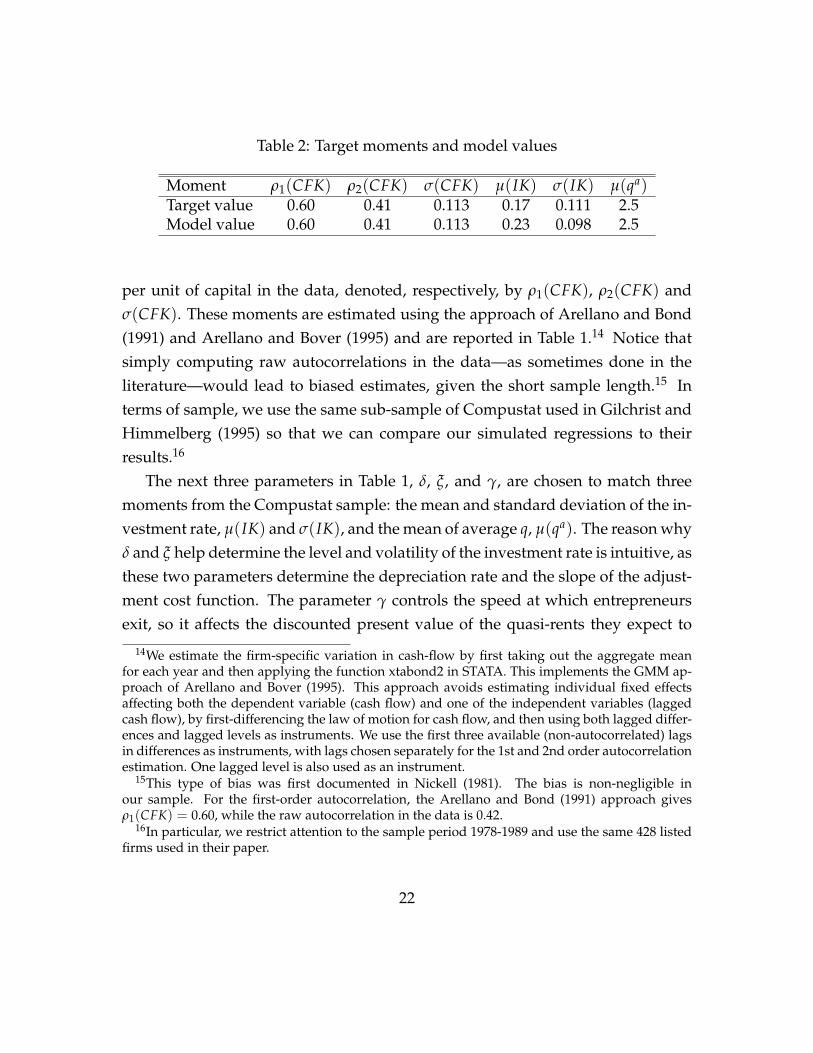
Table 2: Target moments and model values

Moment ρ1(CFK) ρ2(CFK) σ(CFK) µ(IK) σ(IK) µ(qa)Target value 0.60 0.41 0.113 0.17 0.111 2.5Model value 0.60 0.41 0.113 0.23 0.098 2.5

per unit of capital in the data, denoted, respectively, by ρ1(CFK), ρ2(CFK) andσ(CFK). These moments are estimated using the approach of Arellano and Bond(1991) and Arellano and Bover (1995) and are reported in Table 1.14 Notice thatsimply computing raw autocorrelations in the data—as sometimes done in theliterature—would lead to biased estimates, given the short sample length.15 Interms of sample, we use the same sub-sample of Compustat used in Gilchrist andHimmelberg (1995) so that we can compare our simulated regressions to theirresults.16

The next three parameters in Table 1, δ, ξ, and γ, are chosen to match threemoments from the Compustat sample: the mean and standard deviation of the in-vestment rate, µ(IK) and σ(IK), and the mean of average q, µ(qa). The reason whyδ and ξ help determine the level and volatility of the investment rate is intuitive, asthese two parameters determine the depreciation rate and the slope of the adjust-ment cost function. The parameter γ controls the speed at which entrepreneursexit, so it affects the discounted present value of the quasi-rents they expect to

14We estimate the firm-specific variation in cash-flow by first taking out the aggregate meanfor each year and then applying the function xtabond2 in STATA. This implements the GMM ap-proach of Arellano and Bover (1995). This approach avoids estimating individual fixed effectsaffecting both the dependent variable (cash flow) and one of the independent variables (laggedcash flow), by first-differencing the law of motion for cash flow, and then using both lagged differ-ences and lagged levels as instruments. We use the first three available (non-autocorrelated) lagsin differences as instruments, with lags chosen separately for the 1st and 2nd order autocorrelationestimation. One lagged level is also used as an instrument.

15This type of bias was first documented in Nickell (1981). The bias is non-negligible inour sample. For the first-order autocorrelation, the Arellano and Bond (1991) approach givesρ1(CFK) = 0.60, while the raw autocorrelation in the data is 0.42.

16In particular, we restrict attention to the sample period 1978-1989 and use the same 428 listedfirms used in their paper.

22

receive in the future and thus average q. However, the three parameters interact,so we choose them jointly—by a grid search—in order to minimizes the averagesquared percentage deviation between the three model-generated moments andtheir targets. The target moments from the data and the model generated mo-ments are reported in Table 2.17

Notice that there is a tension between hitting the targets for µ(IK) and σ(IK).Increasing any of the parameters, δ, ξ, γ reduces µ(IK), bringing it closer to itstarget value, but also decreases σ(IK), bringing it farther from its target. Noticealso that it is important for our purposes that the model generates a realistic levelof volatility in the investment rate, given that IK is the dependent variable in theregressions we will present in Section 4.3 below.

Our calibration also determines the average size of the wedge between averageand marginal q. In particular, µ(qa) = 2.5 is the mean value of average q while ξ

and µ(IK) determine the mean value of marginal q, which is 1 + ξ(µ(IK)− δ) =

1.25. Therefore, the average wedge between average and marginal q is 1.25. Sincethe presence of the wedge is what breaks the sufficient statistic property of q it isuseful that our calibration imposes some discipline on the wedge’s size.

All the simulations assume that entrepreneurs enter the economy with a unitendowment of capital and zero financial wealth (i.e., zero current profits and zerodebt). Since the entrepreneurs’ problem is invariant to the capital stock and allour empirical targets are normalized by total assets, the choice of the initial capitalendowment is just a normalization. We have experimented with different initialconditions for financial wealth, but they have small effects on our results giventhat—with our parameters—the state variable b converges quickly to its stationarydistribution.

It is useful to compare our results to those of a benchmark model with nofinancial frictions. To make the parametrization of the two models comparable,we re-calibrate the parameters δ, ξ and γ for the frictionless case. The momentsand associated parameters are reported in Table 3. Notice that the frictionlessmodel generates a low value of µ(qa). For given IK, increasing ξ would increase

17The target standard deviation σ(IK) is a pooled estimate.

23

Table 3: Calibration of frictionless model

Parameter δ ξ γ0.05 1.50 0.125

Moment µ(IK) µ(qa) σ (IK)Target value 0.17 2.5 0.111Model value 0.18 1.2 0.116

marginal and average q (which are the same in the frictionless case), but it wouldreduce the volatility of investment.

In Section 4.5 we consider an alternative calibration approach, that targets theaverage finance premium, as defined in equation (15).

4.2 Model dynamics

We now characterize the optimal solution to the entrepreneurs’ problem, first de-scribing optimal choices and values as function of the state variables and nextshowing what this behavior implies for the responses of endogenous variables todifferent shocks.

4.2.1 Characterization

To illustrate the model behavior, it helps intuition to use as state variables A andn, where n is defined as

n ≡ A + 1− δ− b, (29)

rather than using A and b. The variable n is a measure of net worth over assets.Net worth excluding adjustment costs is AK + (1− δ)K− B. Dividing by K leadsto (29).18

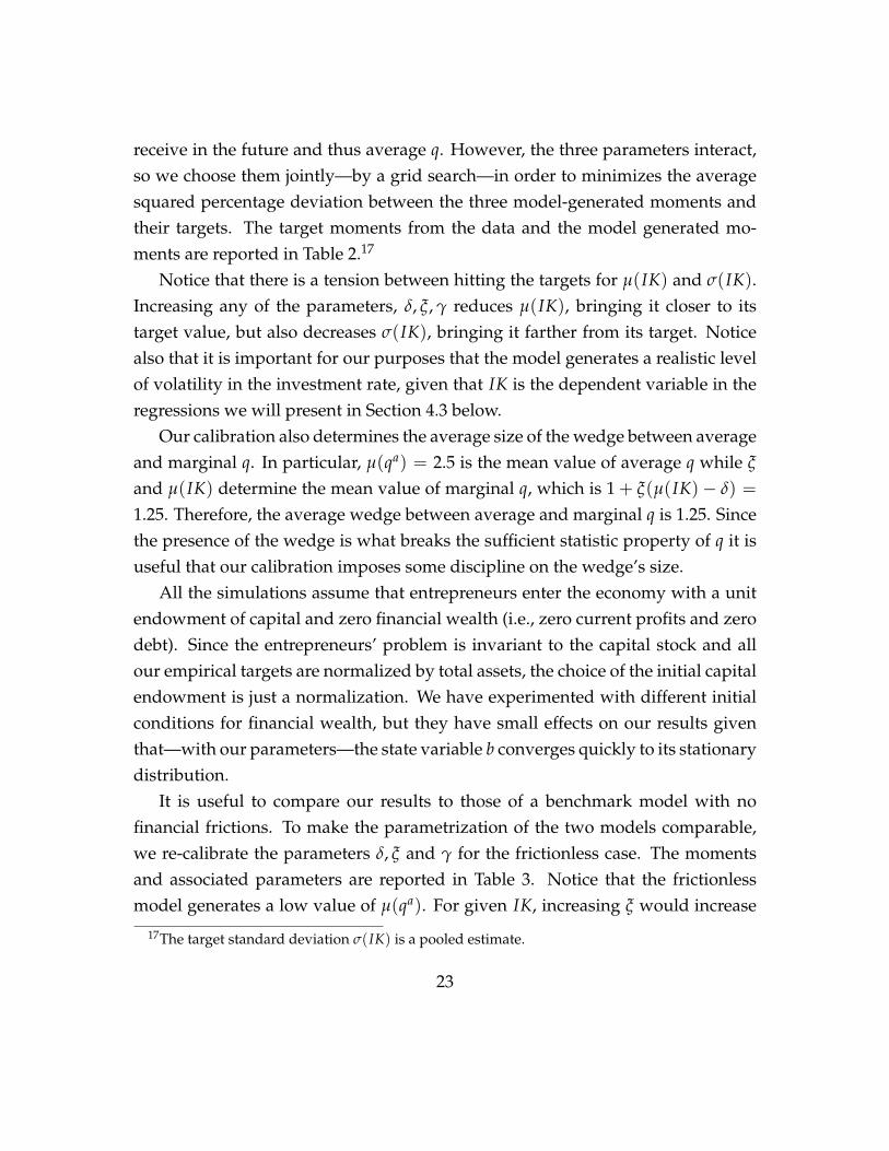
On each row of Figure 1 we plot, respectively, the value function (per unit of

18An alternative is to evaluate installed capital at its shadow value, thus getting net worth equalto AK− G2(K′, K)K− B. The figures are similar.

24

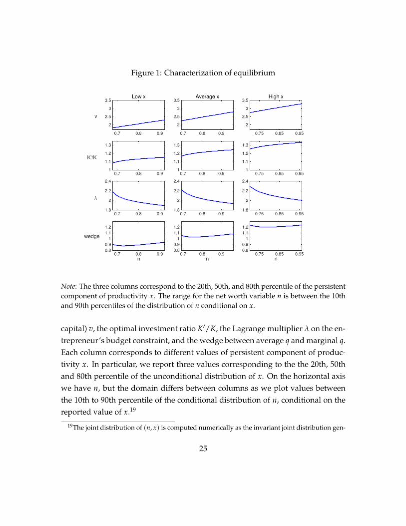
Figure 1: Characterization of equilibrium

0.7 0.8 0.9

v

2

2.5

3

3.5Low x

0.7 0.8 0.9

2

2.5

3

3.5Average x

0.75 0.85 0.95

2

2.5

3

3.5High x

0.7 0.8 0.9

K'/K

1

1.1

1.2

1.3

0.7 0.8 0.91

1.1

1.2

1.3

0.75 0.85 0.951

1.1

1.2

1.3

0.7 0.8 0.9

λ

1.8

2

2.2

2.4

0.7 0.8 0.91.8

2

2.2

2.4

0.75 0.85 0.951.8

2

2.2

2.4

n0.7 0.8 0.9

wedge

0.8

0.9

1

1.1

1.2

n0.7 0.8 0.9

0.8

0.9

1

1.1

1.2

n0.75 0.85 0.95

0.8

0.9

1

1.1

1.2

Note: The three columns correspond to the 20th, 50th, and 80th percentile of the persistentcomponent of productivity x. The range for the net worth variable n is between the 10thand 90th percentiles of the distribution of n conditional on x.

capital) v, the optimal investment ratio K′/K, the Lagrange multiplier λ on the en-trepreneur’s budget constraint, and the wedge between average q and marginal q.Each column corresponds to different values of persistent component of produc-tivity x. In particular, we report three values corresponding to the the 20th, 50thand 80th percentile of the unconditional distribution of x. On the horizontal axiswe have n, but the domain differs between columns as we plot values betweenthe 10th to 90th percentile of the conditional distribution of n, conditional on thereported value of x.19

19The joint distribution of (n, x) is computed numerically as the invariant joint distribution gen-

25

A higher level of n leads to a higher value v and a higher level of investmentK′/K. Moreover, the value function is concave in n. The Lagrange multiplier λ

is equal to the derivative of the value function and therefore is decreasing in n.The fact that λ is decreasing in n reflects the fact that a higher ratio of net worthto capital allows firms to invest more, leading to a higher shadow cost of capitalG1 and thus to a lower expected returns on investment. Eventually, for very highvalues of n we reach λ = 1. However, as the figures show this does not happenfor the range of n values more frequently visited in equilibrium.

The bottom row documents how the wedge varies with the level of net worthn and with the persistent component of productivity x. Let us first look at theeffect of n. Even though λ is decreasing in n, the wedge, qa − qm, does not varymuch with n for a given value of x. Our analytical derivations in Section 2 helpexplain this outcome. Recall from equation (11) that the wedge is equal to

λ− 1λ

βE[v′|s]

.

When we reach the unconstrained solution and λ = 1 the wedge disappears.However, for lower levels of n, for which the constraint is binding, the relationis in general non-monotone. An increase in n reduces the marginal gain from anextra unit of net worth. However, at the same time it increases the future growthrate of firm’s capital stock and so it increases the base to which this marginalquasi-rent is applied. This second effect is captured by the expression E[v′|s],because the value per unit of capital v′ embeds the future growth of the firm andis increasing in n. The plots in the bottom row of Figure 1 show that in the relevantrange of n these two effects roughly cancel.

On the other hand, comparing the values of the wedge across columns, showsthat persistent component of productivity x has large effects on the wedge andthat the wedge is increasing in x. The reason is that higher values of x lead bothto higher values of λ, as the marginal benefits of extra internal funds increasewith productivity, and to higher values of K′/K and v, because higher productiv-

erated by the optimal policies.

26

ity allows the firm to raise more external funds and grow faster. Therefore bothelements of the wedge increase with higher values of x.

4.2.2 Impulse response functions

We now present impulse response functions that illustrate the model dynamicsfollowing the two shocks. To construct these impulse response functions, we takea firm starting at the median values of the state variables n and x. We then subjectthe firm to a shock at time t, simulate 106 paths following the shock, and reportthe difference between the average simulated paths, with and without the initialshock. Given the non-linearity of the model, the initial conditions for n and x ingeneral affect the responses. However, in our simulations these non-linear effectsare relatively small, so the plots below are representative.

In the top panel of Figure 2 we plot the responses of marginal and average q,and cash flow per unit of capital to a 1-standard-deviation persistent shock ε.20

Following a persistent shock all variables increase and return gradually to trend.The response of average q is larger than that of marginal q, thus producing anincrease in the wedge.

In the bottom panel of Figure 2 we plot the responses of the same variablesto a 1-standard-deviation temporary shock η. Also in this case all three variablesrespond positively, but the response is more short-lived. Moreover, now the re-sponse of average q is slightly smaller than the response of marginal q, so thewedge shows a small decrease after the shock.

Notice that average q is a forward-looking variable that incorporates the quasi-rents that the entrepreneur is expected to receive in the future. It is not surprisingthat these quasi-rents are only marginally affected by a temporary shock. In themodel with no adjustment costs, the effect is zero, as shown in Section 3 above.Here, because of adjustment costs, there is a slight positive effect, due to the factthat the investment response displays a small but positive degree of persistence

20The response of investment K′/K is always proportional to the response of marginal q and isthus omitted.

27

Figure 2: Impulse response functions

Time1 2 3 4 5 6 7 8 9 10

0

0.05

0.1

0.15

0.2

0.25

0.3Response to persistent shock

qa

qm

cash flow

Time1 2 3 4 5 6 7 8 9 10

-0.01

0

0.01

0.02

0.03

0.04

0.05Response to temporary shock

qa

qm

cash flow

Note: Average paths following a shock at time 1, in (level) deviations from average pathsfollowing no shock. Cash flow is cash flow per unit of capital.

and high investment in the future increases the future value of installed capital.But this effect is small. In the case of a persistent shock, instead, future quasi-rentsare directly affected by higher future productivity, which is going to lead to fastergrowth (as shown in Figure 1), thus explaining the large increase in qa in the toppanel of Figure 2.

The discussion following Figure 1, helps to explain the response of the wedgeqa − qm. A temporary shock, by increasing A temporarily, leads to a pure increasein net worth per unit of capital, as n = A − b. As we argued when presentingFigure 1, the effect of such an increase on the wedge is in general ambiguous and,with our parameter choices, close to zero. In the case of a persistent shock, instead,the effect is unambiguously to increase the wedge, as the increase in x leads to a

28

higher λ and to a higher E[v′|s].The relative responses of cash flow and marginal q are also different across the

two shocks. In particular, we have a larger response of marginal q relative to thecash flow response in the case of a persistent shock. The reason is that in the caseof a persistent shock the collateral value of capital increases, thus amplifying theeffect on investment.

4.3 Investment regressions

We now turn to investment regressions, and ask whether the model can replicatethe coefficients on q and cash flow observed in the data. In particular, we ask towhat extent does the presence of a financial friction help in obtaining a smallercoefficient on q and a positive and large coefficient on cash flow. To answer thisquestion, we generate simulated data from our model and run investment regres-sions on it. In line with the empirical literature, we generate a balanced panel of500 firms for 20 periods, and run the following investment regression:21

IKit = ai0 + a1qait + a2CFKit + eit, (30)

where we allow for firm-level fixed effects. All reported results are the mean val-ues for 50 simulated panels.

The regression coefficients for the baseline model are presented in the first rowof Table 4. As reference points, in the second row we report the coefficients thatarise in the model without financial frictions and in the last row the empiricalestimates in Gilchrist and Himmelberg (1995), which are representative of the or-ders of magnitude obtained in empirical studies.22 We also report coefficients ofunivariate regressions of investment on average q and cash-flow separately.

The results for the frictionless benchmark are reported in the second line of Ta-

21The model features random exit, so to generate a balanced panel we only keep firms for whichexit does not occur for 20 periods.

22We do not report standard errors, but they are small (less than 0.04) for both coefficients in oursimulated data. They are also small in the empirical estimates of Gilchrist and Himmelberg (1995).

29

Table 4: Investment regressions

Univariate qa Univariate CFKa1 a2 R2 coefficient R2 coefficient R2

Baseline model 0.22 0.15 0.98 0.27 0.98 0.81 0.89Frictionless model 0.67 0.00 1.00 0.67 1.00 0.95 0.86GH (1995) 0.033 0.24 0.05

ble 4. In this case, average q is a sufficient statistic for investment, the coefficienton cash flow is zero and the coefficient on q is equal to the inverse of the adjust-ment cost coefficient ξ, which is calibrated to 1.5. This line shows the standardempirical failure of the benchmark adjustment cost model.

Adding financial frictions helps to get a smaller coefficient on q and a positivecoefficient on cash flow. The effect is sizable, although the coefficient on q is stilllarge compared to the very small numbers found in empirical regressions. Noticealso that the R2 of the regression is very close to 1. This is not surprising given thatwe have a simple two-shock structure and two explanatory variables.23 Giventhat the model is non-linear, the R2 can in general be smaller than 1. However,by experimenting with impulse responses for different initial values of the statevariables we have confirmed that, given our parameter values, the model is closeto linear in its responses to the two shocks, which helps to explain the high R2 inTable 4.

The presence of the wedge breaks the one-to-one relation between q and in-vestment and allows for cash flow to have explanatory power in the the invest-ment regression. In particular, as we saw in Figure 2 the wedge responds in op-posite directions to the two shocks, while qm respond positively to both. So thewedge plays a role somewhat similar to measurement error in dampening the re-gression coefficient. Notice however that the model still features a strong positiverelation between qa and investment, as documented by the fifth and sixth columns

23For the same reason, in the linear model of Example 2, Section 3, the R2 is 1.

30

Table 5: Investment regressions: changing shock variances

Univariate qa Univariate CFKσε ση σ2

η/σ2A a1 a2 R2 coefficient R2 coefficient R2

0.113 0.000 0.00 0.38 -0.48 0.99 0.25 0.99 0.90 0.980.071 0.037 0.11 0.22 0.15 0.98 0.27 0.98 0.81 0.890.033 0.080 0.50 0.28 0.11 0.96 0.32 0.95 0.48 0.560.006 0.107 0.90 0.34 0.10 0.84 0.38 0.75 0.18 0.320.000 0.113 1.00 2.47 0.01 0.92 2.53 0.92 0.11 0.37

of Table 4, which show that a univariate regression between investment and aver-age q produces a large coefficient and a large R2 in simulated data (unlike in actualdata). In the rest of the paper we investigate shock structures that can potentiallyweaken this relation.

4.3.1 The role of the shock structure

It is useful to look at how the shock structure affects investment regressions. InTable 5 we report regression coefficients and R2 for different combinations of σε

and ση, keeping constant the total volatility of At. The second row correspondsto the baseline case of Table 4. In the third column, we report the fraction ofvariance due to the temporary shock. Here we keep all remaining parameters attheir baseline level, since we want to focus on how variance parameters affect ourresult.

The first row of Table 5 shows an extreme case with no temporary shocks. Inthis case, the coefficient on q is larger than in our baseline and the coefficient oncash flow is actually negative. The last row of the table shows the opposite ex-treme, with only temporary shocks. Interestingly, also this row displays a largercoefficient on q. The coefficient on cash flow in this case is close to zero. So going toa one-shock model, worsens the model performance in terms of replicating invest-ment regressions. In this case q and investment tend to comove simply because

31

they are driven by the same shock. In these cases, we get close to the sufficientstatistic result obtained in the one-shock linear model of Example 1. Example 1has indeterminate implications for the coefficients, due to the perfect collinear-ity of q and cash flow. Here, the perfect collinearity result does not hold for tworeasons: first, the model displays inertia so past values of xt determine invest-ment and q, which complicates the correlation structure of investment, q and cashflow; second, the model is non-linear. For these reasons, the bivariate coefficientsare determinate even with a single shock, and, in particular, the model prefers toassign a large coefficient on q.24

The remaining rows of Table 5 illustrate intermediate cases in which bothshocks are present. As argued above, both shocks increase investment but theyhave opposite effects on the wedge and that is what reduces the predictive powerof q. So there is some intermediate mix of shocks that adds maximum noise to theinformation contained in average q and reduces the overall explanatory power ofthe investment regression. In the table this is visible in the non-monotone relationbetween the ratio σ2

η/σ2A and the R2 of the regression.

While it is intuitive that mixing the two shocks affects the total explanatorypower of investment regressions and reduces R2, the quantitative effects on thetwo coefficients a1 and a2 are more complex to interpret, as they also depend onthe magnitudes of the responses of investment, cash flow, and q to the underlyingshocks. In particular, persistent shocks tend to affect more, in relative terms, qthan investment, due to the forward looking nature of q and the presence of thefinancial constraint which dampens the response of investment (see Figure 2). 25

Persistent shocks lead to a smaller response of investment for a given response ofq, when compared to temporary shocks. This is immediately visible in the mono-

24The results in this table may help reconcile our results with the results of Gomes (2001). Inparticular, although Gomes (2001) uses a different model of financial frictions, it is possible thathis result—that q is almost a sufficient statistic for investment—could be driven by his one-shockstructure.

25The same two reasons identified above (inertia and non-linearity) for one-shock models, ex-plain why in the two-shock model the relative size of the two variances matter for the regressioncoefficients, unlike in the simple linearized model with no adjustment costs of Section 3, Example2.

32

tone increase in the univariate coefficient with σ2η/σ2

A. The effect on the bivariatecoefficient a1 is more complex as, at the same time, the presence of temporaryshocks increases the coefficient on cash flow. Therefore, the relation between eachof the coefficients a1 and a2 and the variance ratio σ2

η/σ2A is non-monotone.

The overall take out from Table 5 is that, given all other model parameters, therelative variance of temporary and persistent shocks matter for both the explana-tory power and for the individual coefficients in investment regressions.

4.3.2 The role of parameters

To illustrate how the results depend on the model’s parameters, we now experi-ment with different parameter configurations. In the exercises below we keep allother parameters fixed, i.e., we do not recalibrate the model. Alternative calibra-tions are discussed in Section 4.5. Table 6 documents the investment regressionresults for these alternative specifications.26

The first observation is that our main result is robust to a range of parametervalues: financial frictions reduce the coefficient on average q, a1, (which is equalto 1/ξ in the frictionless case) and produce a positive and sizeable value for thecoefficient on cash flow, a2. Notice also that for all parameter values exploredin this table R2 remains very high for both the multivariate regression and theunivariate regression with average q.

Quantitatively, there are some interesting details. Two parameterizations standout: higher values for β or low values for γ both yield a lower a1 and a higher a2,bringing the model implied regression coefficients closer to their empirical coun-terparts. The reason for these effects is that they magnify the forward-lookingcomponent of q, thus further breaking the link with current investment. How-ever, notice that these values also produce a counterfactually high levels of q onaverage.27 Furthermore, low values of θ or ρx and high values of σA, δ or ξ yield

26When we experiment with different values of β we vary β at the same time, keeping the dif-ference between constant at β− β = 0.02, as in the baseline.

27When we re-calibrate our model starting from β = 0.93, the calibration compensates witha higher value of γ, to hit the average level of q and thus produces coefficients a1 = 0.20 and

33

Table 6: Investment regressions: changing parameters

Univariate qa Univariate CFKa1 a2 R2 coefficient R2 coefficient R2

Baseline 0.22 0.15 0.98 0.27 0.98 0.81 0.89β = 0.910 0.35 0.21 0.98 0.46 0.97 0.80 0.90β = 0.930 0.06 0.16 0.99 0.07 0.98 0.81 0.90θ = 0.200 0.24 0.21 0.98 0.32 0.97 0.79 0.91θ = 0.400 0.16 0.10 0.99 0.18 0.99 0.84 0.87ρx = 0.700 0.24 0.20 0.98 0.32 0.98 0.74 0.91σA = 0.090 0.24 0.18 0.97 0.30 0.96 0.76 0.84σA = 0.130 0.20 0.13 0.99 0.23 0.99 0.84 0.91δ = 0.015 0.12 0.14 0.99 0.14 0.98 0.81 0.89δ = 0.035 0.31 0.17 0.98 0.39 0.97 0.82 0.89ξ = 1.500 0.15 0.11 0.99 0.17 0.99 0.90 0.88ξ = 2.000 0.27 0.18 0.98 0.34 0.97 0.75 0.90γ = 0.085 0.08 0.16 0.99 0.10 0.98 0.81 0.90γ = 0.105 0.33 0.18 0.98 0.41 0.97 0.81 0.89

higher values for both a1 and a2. Finally, it is interesting to note that our modelimplies that a1 is increasing in ξ, which is the opposite of what happens with nofinancial frictions.

4.4 News shocks

We now turn to news shocks. Example 3 in Section 3 shows that in the case ofno adjustment costs news shocks introduce additional noise in average q, thus re-ducing its predictive power. Here we want to investigate whether the same forcesare at work in our full model with adjustment costs and see their quantitativeimplications.

Introducing news shocks increases the number of state variables, since weneed to keep track of anticipated values of xt. Therefore, to simplify computations,

a2 = 0.15, which are very close to our baseline results.

34

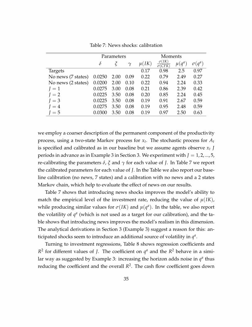
Table 7: News shocks: calibration

Parameters Momentsδ ξ γ µ(IK) σ(IK)

σ(CFK) µ(qa) σ(qa)

Targets 0.17 0.98 2.5 0.97No news (7 states) 0.0250 2.00 0.09 0.22 0.79 2.49 0.27No news (2 states) 0.0200 2.00 0.10 0.22 0.94 2.24 0.33J = 1 0.0275 3.00 0.08 0.21 0.86 2.39 0.42J = 2 0.0225 3.50 0.08 0.20 0.85 2.24 0.45J = 3 0.0225 3.50 0.08 0.19 0.91 2.67 0.59J = 4 0.0275 3.50 0.08 0.19 0.95 2.48 0.59J = 5 0.0300 3.50 0.08 0.19 0.97 2.50 0.63

we employ a coarser description of the permanent component of the productivityprocess, using a two-state Markov process for xt. The stochastic process for At

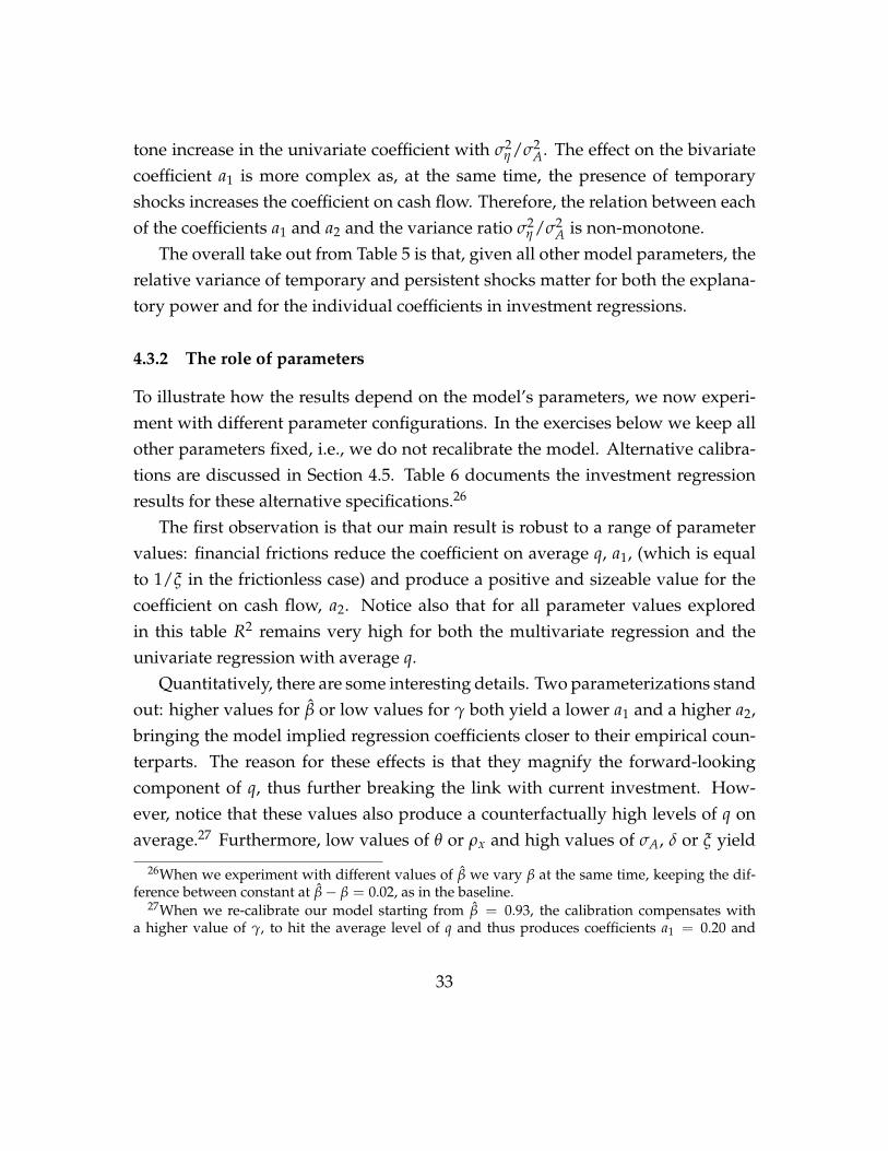
is specified and calibrated as in our baseline but we assume agents observe xt Jperiods in advance as in Example 3 in Section 3. We experiment with J = 1, 2, ..., 5,re-calibrating the parameters δ, ξ and γ for each value of J. In Table 7 we reportthe calibrated parameters for each value of J. In the Table we also report our base-line calibration (no news, 7 states) and a calibration with no news and a 2 statesMarkov chain, which help to evaluate the effect of news on our results.

Table 7 shows that introducing news shocks improves the model’s ability tomatch the empirical level of the investment rate, reducing the value of µ(IK),while producing similar values for σ(IK) and µ(qa). In the table, we also reportthe volatility of qa (which is not used as a target for our calibration), and the ta-ble shows that introducing news improves the model’s realism in this dimension.The analytical derivations in Section 3 (Example 3) suggest a reason for this: an-ticipated shocks seem to introduce an additional source of volatility in qa.

Turning to investment regressions, Table 8 shows regression coefficients andR2 for different values of J. The coefficient on qa and the R2 behave in a simi-lar way as suggested by Example 3: increasing the horizon adds noise in qa thusreducing the coefficient and the overall R2. The cash flow coefficient goes down

35

Table 8: News shocks: investment regressions

a1 a2 R2

GH (1995) 0.033 0.24No news (7 states) 0.2047 0.1530 0.984No news (2 states) 0.2434 0.0829 0.985J = 1 0.1920 −0.0121 0.982J = 2 0.1774 0.0161 0.974J = 3 0.1417 0.0502 0.978J = 4 0.1467 0.0628 0.976J = 5 0.1394 0.0824 0.971

when going from no news to 1 period anticipation, and then increases monotoni-cally in J.

Comparing the cases of no news and the case J = 5, the overall take awayfrom Tables 7 and 8 is that news shocks improve the model’s ability to match theobserved behavior of investment, q and cash flow, both in terms of levels andvolatility and in terms of the cross-correlations captured by investment regres-sions. The central intuition is that news shocks introduce a source of variation inq due to anticipated future shocks, which have little bearing on the contempora-neous movements in investment.

Due to the use of a 2 state Markov chain, the model with news does worsethan the baseline in terms of the cash flow coefficient, so it is an open quesitonfor future work whether increasing the state space and possibly using alternativemodels of anticipated news that economize on state variables can further improvethe model’s empirical performance.28

4.5 Targeting the mean finance premium

In this section we consider an alternative calibration in which we add to our targetmoments the mean finance premium, µ( f p). Following Bernanke et al. (1999) we

28See for example the information structure in Blanchard et al. (2013).

36

Table 9: Targeting the finance premium

Parameters:δ ξ γ

0.1300 2.00 0.005Moments:

µ(IK) µ(qa) σ(IK) µ( f p)Target 0.17 2.5 0.111 0.020Model 0.24 2.2 0.096 0.024Investment regression:

a1 a2 R2

0.19 0.22 0.99

choose a target for µ f p of 2%. In particular, we now choose the parameters δ, ξ,and γ to minimize the average squared percentage deviation of the four momentstargeted. The main reason for this robustness check is to ensure that our resultsdo not rely on an implausibly high value of the external finance premium.

Parameter values, model moments and regression results for this calibrationare reported in Table 9. Overall, the results are similar to the baseline, except thiscalibration delivers a larger coefficient on a2. In particular, a useful observationis that the model does not need to rely on a high external finance premium toproduce a large wedge between average and marginal q.

5 Conclusions

The paper shows that financial frictions can help dynamic investment modelsmove closer to the correlations observed in the data. The model in this paperis stylized, but we think our main conclusions on the role of different shocks willextend to more complex models. In particular, we think it is a promising avenueto build models where a substantial fraction of the volatility in q is associated tonews about profitability relatively far in the future and where these news have rel-

37

atively small effects on current investment decisions. By assuming risk neutrality,we have omitted an important source of volatility in asset prices, namely volatilityin discount factors and risk premia. It is an important open question how theseadditional sources of volatility affect the correlations investigated here, especiallybecause these factors are likely to correlate with the stringency of financial con-straints for individual firms.

References

Abel, A. B. and Eberly, J. C. (2011). How q and cash flow affect investment withoutfrictions: An analytic explanation. The Review of Economic Studies, 78(4):1179–1200.

Abel, A. B. and Eberly, J. C. (2012). Investment, valuation, and growth options.Quarterly Journal of Finance, 2.

Albuquerque, R. and Hopenhayn, H. A. (2004). Optimal lending contracts andfirm dynamics. The Review of Economic Studies, 71(2):285–315.

Alti, A. (2003). How sensitive is investment to cash flow when financing is fric-tionless? Journal of Finance, 58:707–722.

Arellano, M. and Bond, S. (1991). Some tests of specification for panel data: Montecarlo evidence and an application to employment equations. The Review of Eco-nomic Studies, 58(2):277–297.

Arellano, M. and Bover, O. (1995). Another look at the instrumental variable esti-mation of error-components models. Journal of Econometrics, 68(1):29 – 51.

Atkeson, A. and Cole, H. (2005). A dynamic theory of optimal capital structureand executive compensation. Working Paper 11083, National Bureau of Eco-nomic Research.

38

Bernanke, B. S., Gertler, M., and Gilchrist, S. (1999). The financial accelerator in aquantitative business cycle framework. In Handbook of Macroeconomics, volume1, Part C, pages 1341 – 1393. Elsevier.

Biais, B., Mariotti, T., Plantin, G., and Rochet, J.-C. (2007). Dynamic security de-sign: Convergence to continuous time and asset pricing implications. The Re-view of Economic Studies, 74(2):345–390.

Blanchard, O. J., de Silanes, F. L., and Shleifer, A. (1994). What do firms do withcash windfalls? Journal of Financial Economics, 36(3):337 – 360.

Blanchard, O. J., L’Huillier, J.-P., and Lorenzoni, G. (2013). News, noise, and fluc-tuations: An empirical exploration. American Economic Review, 103(7):3045–70.

Cao, D. (2013). Speculation and financial wealth distribution under belief hetero-geneity. Georgetown University Working Paper.

Clementi, G. L. and Hopenhayn, H. A. (2006). A theory of financing constraintsand firm dynamics. The Quarterly Journal of Economics, 121(1):229–265.

Cooley, T., Marimon, R., and Quadrini, V. (2004). Aggregate consequences of lim-ited contract enforceability. Journal of Political Economy, 112(4):817–847.

Cooper, R. and Ejarque, J. (2003). Financial frictions and investment: requiem inq. Review of Economic Dynamics, 6(4):710 – 728. Finance and the Macroeconomy.

DeMarzo, P. M., Fishman, M. J., He, Z., and Wang, N. (2012). Dynamic agencyand the q theory of investment. The Journal of Finance, 67(6):2295–2340.

DeMarzo, P. M. and Sannikov, Y. (2006). Optimal security design and dynamiccapital structure in a continuous-time agency model. The Journal of Finance,61(6):2681–2724.

Di Tella, S. (2016). Uncertainty shocks and balance sheet recessions. StanfordUniversity Working Paper.

39

Eberly, J., Rebelo, S., and Vincent, N. (2008). Investment and value: A neoclassicalbenchmark. Working Paper 13866, National Bureau of Economic Research.

Fazzari, S. M., Hubbard, R. G., and Petersen, B. C. (1988). Financing constraintsand corporate investment. Brookings Papers on Economic Activity, 1988(1):141–206.

Gilchrist, S. and Himmelberg, C. P. (1995). Evidence on the role of cash flow forinvestment. Journal of Monetary Economics, 36(3):541 – 572.

Gomes, J. F. (2001). Financing investment. American Economic Review, 91(5):1263–1285.

Hayashi, F. (1982). Tobin’s marginal q and average q: A neoclassical interpreta-tion. Econometrica, 50(1):pp. 213–224.

He, Z. and Krishnamurthy, A. (2013). Intermediary asset pricing. American Eco-nomic Review, 103(2):732–70.

Hennessy, C. A. and Whited, T. M. (2007). How costly is external financing? evi-dence from a structural estimation. The Journal of Finance, 62(4):1705–1745.

Hubbard, R. G. (1998). Capital-market imperfections and investment. Journal ofEconomic Literature, 36(1):193–225.

Kaplan, S. N. and Zingales, L. (1997). Do investment-cash flow sensitivities pro-vide useful measures of financing constraints? The Quarterly Journal of Eco-nomics, 112(1):169–215.

Kiyotaki, N. and Moore, J. (1997). Credit cycles. Journal of Political Economy,105(2):211–248.

Moyen, N. (2004). Investment-cash flow sensitivities: Constrained versus uncon-strained firms. The Journal of Finance, 59(5):2061–2092.

40

Nickell, S. (1981). Biases in dynamic models with fixed effects. Econometrica,49(6):1417–1426.

Rampini, A. A. and Viswanathan, S. (2013). Collateral and capital structure. Jour-nal of Financial Economics, 109(2):466 – 492.

Rauh, J. D. (2006). Investment and financing constraints: Evidence from the fund-ing of corporate pension plans. The Journal of Finance, 61(1):33–71.

Sargent, T. J. (1980). Tobin’s q and the rate of investment in general equilibrium.Carnegie-Rochester Conference Series on Public Policy, 12:107 – 154.

Schiantarelli, F. and Georgoutsos, D. (1990). Monopolistic competition and the qtheory of investment. European Economic Review, 34(5):1061 – 1078.

41

A Appendix

A.1 Proofs for Section 2

Proof of Proposition 2. The envelope condition for K is

v (b, s) = λ(

A (s)− G2(K′, K

)− b)

.

Substituting in (9) and using time subscripts, we get

λtG1,t = βλtEt [bt+1] + βEt [λt+1 (At+1 − G2,t+1 − bt+1)] , (31)

which, rearranged, gives (13). Notice that (12) and µt ≥ 0 imply

Et[(βλt − βλt+1)bt+1

]≥ 0.

So (31) impliesG1,tλt ≥ βEt [λt+1 (At+1 − G2,t+1)] ,

which yields the first inequality in (14). Moreover, (12) also implies

Et[βλt (At+1 − G2,t+1 − bt+1)

]≤ Et [βλt+1 (At+1 − G2,t+1 − bt+1)] ,

which, together with (31), gives the second inequality in (14).

A.2 Proofs for Section 3

Proof of Lemma 1. Let B be the space of bounded functions f : S/sr → [1, ∞).Define the map T : B→ B as follows

T f (s) = (1− θ) β(1− γ)E [ f (s′) R (s′) |s, s′ 6= sr] + γR (sr)

1− θβE [R(s′)|s].

42

Let us first check that T f ∈ B if f ∈ B, so the map is well defined. Notice thatconditions (18)-(19) and β < β imply that

(1− θ) βE [R (s′) |s]1− θβE [R (s′) |s]

> 1.

Then for any f ∈ B we have

T f (s) ≥ (1− θ) βE [R (s′) |s]1− θβE [R (s′) |s]

> 1, (32)

showing that T f (s) ≥ 1.Next, we show that T satisfies Blackwell’s sufficient conditions for a contrac-

tion. The monotonicity of T is easily established. To check that it satisfies thediscounting property notice that if f ′ = f + a, then

T f ′ (s)− T f (s) =(1− γ) (1− θ) βE [R (s′) |s, s 6= sr]

1− θβE [R (s′) |s]a < ζa,

where the inequality follows from assumption (20). Since T is a contraction aunique fixed point f exists. Set Λ(s) = f (s) for all s 6= sr. Inequality (32) showsthat Λ (s) > 1 for all s 6= sr, completing the proof.

Proof of Proposition 3. Let Λ be defined as in Lemma 1. We proceed by guessingand verifying that the value function has the form (16). Under this conjecture, theno-default condition (4) can be rewritten in the form

B′(s′) ≤ θR(s′)K′.

Therefore, we can rewrite problem (2) as

maxC,K′,B′(.)

C + β ∑s′

π(s′|s) [

Λ(s′) (

R(s′)

K′ − B′(s′))]

43

s.t. C + K′ ≤ R (s)K− B + β ∑s′

π(s′|s)B′(s′), (λ)

B′(s′)≤ θR

(s′)

K′ for all s′, (µ(s′)

π(s′|s))

C ≥ 0, (τc)

K ≥ 0, (τk)

where, in parenthesis, we report the Lagrange multiplier associated to each con-straint. The multipliers of the no-default constraints are normalized by the prob-abilities π (s′|s). The first-order conditions for this problem are

1− λ + τc = 0,

βE[Λ(s′)R(s′)|s

]− λ + θE

[µ(s′)R(s′)|s

]+ τk = 0,

−βΛ(s′)π(s′|s)+ λβπ

(s′|s)− µ

(s′)

π(s′|s)= 0.

We want to show that the values for C, K′, B′ in the statement of the propositionare optimal. It is immediate to check that they satisfy the problem’s constraints.To show that they are optimal we need to show that τc = λ− 1 > 0, τk = 0, andµ (s′) > 0 for all s′. Setting τk = 0 the second and third first-order conditions giveus

λ =(1− θ) βE [Λ(s′)R(s′)]

1− θβE [R′(s′)]

which, by construction, is equal to Λ (s). Then we have

τc = Λ (s)− 1 > 0,

which follows from Lemma 1,

µ(s′)= βΛ (s)− βΛ

(s′)> 0,

which follows from condition (22). Substituting the optimal values in the objectivefunction we obtain Λ (s) (R (s)K− B) confirming our initial guess.

44

Proof of Proposition 5. First we derive the formula (28) for average q. From formula(26) we have

qat =

[β (1− θ) (γ + (1− γ) Λ) + θβ

]Et[At+1

]+ β (1− θ) (1− γ)REt

[Λt+1

]=[β (1− θ) (γ + (1− γ) Λ) + θβ

]xt+1

+ β (1− θ) (1− γ)RΛEt

[1

1− θβR

∞

∑j=0

((1− γ) Λ

γ + (1− γ) Λ

)j

Et+1

[xt+1+j

R

]],

where the last equality comes from formula (27) and the fact that xt+1 is knownat time t and ηt+1+j is not known at t for all j ≥ 0. Now simplify the second termusing the dynamic equation for xt+1+j:

xt+1+j = ρjxt+1 +j

∑j′=1

ρj−j′εt+1+j′ .

By using this expression and simplify the algebra, we obtain:

Et

[1

1− θβR

∞

∑j=0

((1− γ) Λ

γ + (1− γ) Λ

)j

Et+1[xt+1+j

]]

=1

1− θβR1

1− (1−γ)Λρ

γ+(1−γ)Λ

xt+1

+Et

[1

1− θβR

∞

∑j=0

((1− γ) Λ

γ + (1− γ) Λ

)j j

∑j′=1

ρj−j′εt+1+j′

].

Using the fact that Et

[εt+1+j′

]= 0 for all j′ > J − 1 and Et

[εt+1+j′

]= εt+1+j′ for

45

j′ ≤ J − 1, the second term becomes

Et

[1

1− θβR

∞

∑j=0

((1− γ) Λ

γ + (1− γ) Λ

)j j

∑j′=1

ρj−j′εt+1+j′

]

= Et

[1

1− θβR

∞

∑j′=1

∞

∑j=j′

((1− γ) Λ

γ + (1− γ) Λ

)j

ρj−j′εt+1+j′

]

=1

1− θβR

J−1

∑j′=1

((1− γ) Λ

γ + (1− γ) Λ

)j′

εt+1+j′1

1− (1−γ)Λρ

γ+(1−γ)Λ

.

This equality combined with the derivation for qat above implies (28).

Now we compute regression coefficients and R2 for the regression of ˜IKt onAt and qa

t . Let yt = ˜IKt and Xt =[

At qat

]. To simplify the algebra write the

equations for ˜IKt and qt as follows:

˜IKt = αi1At + αi2xt+1

qat = αqxt+1 + εt

We can then compute

E[ytXt] =[(αi1 + αi2ρ) σ2 + α1σ2

η (αi1 + αi2ρ) αqρσ2 + αi2αqσ2ε

],

E[XtX′t] =

[σ2 + σ2

η αqρσ2

αqρσ2 α2qσ2 + σ2

ε

],

andE[y2

t ] = (αi1 + αi2ρ)2 σ2 + α2i2σ2

ε + αi1σ2η ,

where σ2 = var(xt) = (1− ρ2)σ2ε and σ2

ε = var(εt).The coefficients on cash flow and qa

t are given by:

1det(E[XtX′t])

[α2

qσ2 + σ2ε −αqρσ2

−αqρσ2 σ2 + σ2η

]E[ytXt],

46

and, after some algebra, we get the coefficient on qa, which is

αi2αq

(σ2

ηρ2σ2 +(

σ2 + σ2η

)σ2

ε

)α2

qσ4(1− ρ2) + σ2η(α

2qσ2 + σ2

ε ) + σ2σ2ε

,

and is immediately decreasing in σ2ε . Similarly, we can derive the coefficient on

At, which is

σ2ε

((αi1 + αi2ρ) σ2 + αi1σ2

η

)+ αi1α2

qσ2(

σ2ε + σ2

η

)α2

qσ4(1− ρ2) + σ2η(α

2qσ2 + σ2

ε ) + σ2σ2ε

.

Rewrite this expression as

A1 + A2σ2ε

A3 + A4σ2ε=

A2

A4+

A1A4 − A2A3

A4 (A3 + A4σ2ε )

,

where A1, A2, A3, A4 > 0. Direct algebra yields

A1A4 − A2A3 = −α2qσ2ραi2σ2

ε

(σ2 + σ2

η

)− α2

qσ2αi2ρσ2ρ2σ2η < 0.

Therefore the coefficient on cash flow is strictly increasing in σ2ε .

Finally, the R2 is

R2 =E[ytXt]E[XtX′t]

−1E[X′tyt]

E[y2t ]

,

which can be written as

R2 =B1 + B2σ2

ε

B3 + B4σ2ε=

B2

B4+

B1B4 − B2B3

B4 (B3 + B4σ2ε )

,

where B1, B2, B3, B4 > 0. In order to show that R2 is decreasing in σ2ε , we only

47

need to show that B1B4 − B2B3 > 0. After some algebra we obtain

B1B4 − B2B3 =

σ2ηα2

i2ρ2σ2α2qσ2

ηρ2σ2 +(

σ2 + σ2η

)α2

i2σ2ε α2

q

(σ2

ηρ2σ2 +(

σ2(1− ρ2) + σ2η

)σ2

ε + ρ2σ2(

σ2 + σ2η

))> 0.

A.3 Numerical Algorithm

With slight abuse of notation, let v(n, s) denote the value function as a function ofnet worth net of adjustment costs n = A + 1− δ− b instead of as a function of b.

The main complication in the computation is that at each iteration we haveto solve for an optimal state-contingent portfolio choice because the entrepreneurcan choose b′ (s′) for each s′. Let λ denote the multiplier on the budget constraint(6). The envelope condition implies vn (s, n) = 1 + λ. Moreover

β (1 + λ) ≥ βvn(

A(s′)+ 1− δ− b′

(s′)

, s′)

v(

A(s′)+ 1− δ− b′

(s′)

, s′)≥ (1− θ) v

(A(s′)+ 1− δ, s′

). (33)

with at least one of the two inequalities holds with equality. These two equationsdetermine b′ (s′) as a function of λ. To determine k′ we have:

G1(k′, 1

)(1 + λ) = βE

[b′(s′)|s](1 + λ) + βE

[v(

A(s′)+ 1− δ− b′

(s′)

, s′)|s]

(34)so k′ is a function of λ. Notice that in order to solve for the optimal decisionsb (s′) and k′ we need to invert the first derivative: vn. Numerical derivative iscomputationally time consuming and imprecise. Thus in each iteration of thealgorithm, we solve for both v and vn.

Lastly, to compute λ, we use

A (s) + 1− δ− b + βE[b′(s′)|s]

k′ − G(k′, 1

) { = 0 if λ > 0> 0 if λ = 0

,

48

where b′ (s′) an k′ are determined from (33) and (34) given λ.

49