Investment: Tobin's q - Lecture 10, ECON 4310 Tobin’s q Lecture 10, ECON 4310 ... Today’s...

. . . . . .

.

......

Investment: Tobin’s qLecture 10, ECON 4310

Tord Krogh

September 16, 2013

Tord Krogh () ECON 4310 September 16, 2013 1 / 48

. . . . . .

Why investment?

Today’s lecture is devoted to the theory of investment. Why? Because investment behavior is animportant determinant for:

Long run growth (through the role of capital)

Business cycle dynamics


. . . . . .

Investment over the business cycle

Investments are highly correlated with the business cycle and a lot more volatile than output.Here we have plots for the cyclical components of mainland GDP and oil investments for Norway(cyclical? Next lecture!). There are two lines because I have used two different measures of thecyclical component.

1980 1985 1990 1995 2000 2005 2010

-0.04

-0.02

0.00

0.02

0.04

0.06

0.08

(a) Mainland GDP

1980 1985 1990 1995 2000 2005 2010

-0.6

-0.4

-0.2

0.0

0.2

0.4

(b) Oil investments


. . . . . .

Investment over the business cycle II

The investment components are by far the most volatile time series (again: cyclical components).

Variable Standard deviationMainland GDP 2.49

Consumption 2.38Public consumption 1.58

Investments except oil 9.96Residential investment 10.48

Oil investment 14.77

Exports (except oil sector) 4.50Imports (except oil sector) 5.57


. . . . . .

So: What determines the rate of investment?

In the very first macro models you were taught, investment plays an important role over thebusiness cycle. A typical Keynesian investment function is:

It = a0 + a1Yt − a2rt

where It is investment, Yt is GDP and rt is the real interest rate. So: Investment should behigher when the interest rate is low, and vice versa.


. . . . . .

So: What determines the rate of investment? II

A similar view is found in typical central bankers’ view of how monetary policy affects inflation(illustration from Norges Bank’s website):


. . . . . .

So: What determines the rate of investment? III

However, ever since Haavelmo (1960) (A Study in the Theory of Investment), it has beenrecognized that the Keynesian investment function is inconsistent with the simpleneoclassical model of investment.

Moene and Rødseth (1991): Haavelmo’s aim in this book was to “destroy the standardKeynesian demand function for investment”, and “to offer an alternative”.

Main point: Neoclassical theory only predicts a relationship between the desired stock ofcapital and the interest rate. No reason to expect a smooth relationship betweeninvestments and the interest rate.


. . . . . .

So: What determines the rate of investment? IV

Using a simple neoclassical model it is indeed possible to generate data series where the rate ofinvestment is declining in the interest rate.

6 7 8 9 10 11 12 130.2

0.25

0.3

0.35

0.4

0.45

0.5

Leve

l of i

nves

tmen

t

Capital rental rate

Figure: Scatter plot: Rate of investment as a function of the interest rate


. . . . . .

So: What determines the rate of investment? V

But the previous figure was just a coincidence for the first 20 observations. When I generatelonger time series we see that the true relationship is much less smooth:

2 2.5 3 3.5 4 4.5 5 5.5 6 6.5 7−20

−15

−10

−5

0

5

10

15

Leve

l of i

nves

tmen

t

Capital rental rate

Figure: Scatter plot: Rate of investment as a function of the interest rate


. . . . . .

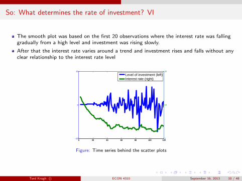
So: What determines the rate of investment? VI

The smooth plot was based on the first 20 observations where the interest rate was fallinggradually from a high level and investment was rising slowly.

After that the interest rate varies around a trend and investment rises and falls without anyclear relationship to the interest rate level

0 20 40 60 80 100 120−20

0

20

0 20 40 60 80 100 1200

10

20

Level of investment (left)Interest rate (right)

Figure: Time series behind the scatter plots


. . . . . .

So: What determines the rate of investment? VII

Indeed, if we plot the rate of investment as a function of the change in the interest rate, it seemslike we are much closer to an accurate description:

−0.8 −0.6 −0.4 −0.2 0 0.2 0.4 0.6 0.8−15

−10

−5

0

5

10

15

20

Leve

l of i

nves

tmen

t

Change in interest rate

Figure: Scatter plot: Rate of investment as a function of the change in the interest rate


. . . . . .

Neoclassical theory of investment

Outline

...1 Neoclassical theory of investment

...2 Capital adjustment costs: Tobin’s q

...3 Tobin’s q and the stock-market value

...4 Summary


. . . . . .


The value of a firm

Today we focus solely at firm’s investment behavior. But firms are owned by households, and (atleast as a starting point) we should assume that firm managers maximize the value of the firm forits owners.

Let Vs denote the value of a firm at the end of period s

Owners of the firm from the end of period s receive dividends ds+1 in the next period, andcan sell the firm at a value Vs+1

Assuming that there exists a risk free interest rate r , we know that the value in a perfectforesight case must satisfy:

1 + r =ds+1 + Vs+1

Vs


. . . . . .


The value of a firm II

Rewriting and then iterating forward we have:

Vt =T∑

s=t+1

(1

1 + r

)s−t

ds +

(1

1 + r

)T

Vt+T

The no-bubble condition is limT→∞

(1

1+r

)TVt+T = 0, and with that imposed we get:

Vt =∞∑

s=t+1

(1

1 + r

)s−t

ds

⇒ The value of a firm reflects the NPV of future dividends.

When making decisions, the firm manager should be concerned with maximizing the sum ofdividends paid today plus the value at the end of period t: Vt + dt , so the objective functionshould be:

dt + Vt =∞∑s=t

(1

1 + r

)s−t

ds


. . . . . .


Firm behavior

Lets assume a production function AtF (Kt , Lt). The firm hires labor but purchases its owncapital (i.e. not rental market for capital). With no depreciation of capital, its profits in period twhich are paid as dividends are:

dt = AtF (Kt , Lt)− wtLt − [Kt+1 − Kt ]

The firm manager thus chooses {Ls ,Ks+1}∞s=t to maximize:

∞∑s=t

(1

1 + r

)s−t

{AsF (Ks , Ls)− wsLs − [Ks+1 − Ks ]}

taking Kt as given. First-order conditions:

AsF′L(Ks , Ls) = ws

for s ≥ t andAsF

′K (Ks , Ls) = r

for s > t.


. . . . . .


Firm behavior II

How does this give us a theory of investment? Well, since It = Kt+1 − Kt , the rate of investmentdepends on what capital levels that come out of the first order conditions. Assume, for simplicity,that we are in a full employment equilibrium so Ls = L̄ for all s. Then the first-order condition forlabor just determines the real wage while

AsF′K (Ks , L̄) = r

defines the optimal capital stock as a function of productivity and the interest rate, K∗(As , r).The rate of investment is then:

Is = K∗(As+1, r)− K∗(As , r)


. . . . . .


Firm behavior III

To see how the interest rate affects investment we need to see how K∗ changes:

dK∗

dr=

r

AF ′′KK (K

∗, L̄)

which is negative under standard assumptions. We therefore have:

Holding Kt constant, It will fall if r goes up since Kt+1 falls

But an increase in the interest rate level for all periods (or a change in the interest rate path)will affect both present and future capital! No reason to expect a smooth relationshipbetween investment and the interest rate. Might be that investment can be both high andlow for the same rate of interest.

More important whether the interest rate is rising or falling, since that determines whetherthe capital stock is being decreased or increased.

This was one of the main points of Haavelmo (1960). Explains why the Keynesian investmentfunction is inconsistent with a neoclassical theory of investment.


. . . . . .


Problem: Infinite investment

While this helps us understand the weakness of a Keynesian investment function, Haavelmoand others have pointed out that the basic neoclassical theory has a big problem as well.

Best understood in a continuous time setup. First-order condition for capital is then basicallythe same:

A(s)F ′K (K(s), L̄) = r

while investment is I (s) = dK(s)ds

= K̇(s).

By implicitly differentiating the first-order condition we find K∗ as a smooth function of r .

So discrete changes in the interest rate must lead to discrete changes in the capital stock

⇒ Discrete changes in the interest rate cause an infinite rate of investment!

This is another argument against the Keynesian function: Investment cannot be a smoothfunction of the interest rate.

But it is also a problem for the basic model: The rate of investment is clearly not infinite inpractice

In a discrete time model we of course don’t find infinite investment, but that is just camouflage.


. . . . . .


Problem: Infinite investment II

Put differently, the Keynesian investment function makes investment too smooth

But the neoclassical model, although staring in the “right” place, predicts too rapid changesin investment.

⇒ Need to combine the neoclassical setup with a story for why investment is slower to adjustthan in the baseline case

⇒ Natural solution: Add capital adjustment costs – which is what we will look at today

⇒ Haavelmo’s solution: Build a model where investors are rationed in booms and invest zero inrecessions


. . . . . .

Capital adjustment costs: Tobin’s q

Outline




...4 Summary


. . . . . .


Capital adjustment costs

Will now present a model with adjustment cost based on the presentation in Obstfeld and Rogoff(Chapter 2.5, 1996). Romer’s presentation is less suitable since it uses control theory. Advice foryou: Learn the model as it is presented in this lecture, but use Romer’s discussion of the modelfor improved understanding. (Only Romer chapter 8.1-8.6 (3rd edition) that is on the syllabus).


. . . . . .


Capital adjustment costs II

In the baseline case the firm could purchase or sell capital with no cost other than the capitalitself. Assume instead that capital is costly to adjust because of installation costs, productiondisruption, learning, etc. Profits in period s are given by:

AsF (Ks , Ls)− wsLs − Is −χ

2

I 2sKs

where Is = Ks+1 − Ks . Adjustment costs are convex, so it is costly to adjust a lot at the time.Why relative to capital? Both intuitive and convenient for the analytical results.


. . . . . .


Capital adjustment costs III

The firm now chooses capital and the rate of investment to maximize (we assume Ls = L̄ forsimplicity):

Vt =∞∑s=t

(1

1 + r

)s−t [AsF (Ks , L̄)− ws L̄− Is −

χ

2

I 2sKs

]subject to Ks+1 = Ks + Is . Let qs be the current-valued Lagrange multiplier. Lagrangianexpression:

Lt =∞∑s=t

(1

1 + r

)s−t [AsF (Ks , L̄)− ws L̄− Is −

χ

2

I 2sKs

− qs(Ks+1 − Ks − Is)

]First-order conditions:

Is : − χIs

Ks− 1 + qs = 0

Ks+1 : − qs +1

1 + r

(As+1FK (Ks+1, L̄) +

χ

2

(Is+1

Ks+1

)2

+ qs+1

)= 0


. . . . . .


Capital adjustment costs IV

The Lagrange multiplier q plays a central role (yes, this is Tobin’s q). As any other Lagrangemultiplier, it is a shadow price. In this case, qs is the shadow price of capital in place at the endof period s. From the first-order condition with respect to investment we see that:

qs = 1 + χIs

Ks

Under the optimal plan, the firm invests such that the marginal cost of an additional unit ofcapital (which equals 1 plus the adjustment cost) must equal the shadow price of capital. Canalso write this as the investment equation that Tobin (1969) posited:

Is = (qs − 1)Ks

χ

So investment is only positive when qs > 1, i.e. when the shadow price of capital exceeds theprice of new capital (before adjustments costs).


. . . . . .


Capital adjustment costs V

Next consider the first-order condition with respect to future capital.

qs =1

1 + r

(As+1FK (Ks+1, L̄) +

χ

2

(Is+1

Ks+1

)2

+ qs+1

)

This is like an investment Euler condition. The shadow price of capital today must equal thediscounted value of

the return of capital next period,

what you save in adjustment costs next period

the future shadow price (since capital can be sold next period).


. . . . . .


Capital adjustment costs VI

In the same way as we used iterative substitution to rewrite the value of a firm, we can imposelimT→∞

qt+T

(1+r)T= 0 (i.e. no bubble) and get:

qt =∞∑

s=t+1

(1

1 + r

)s−t[AsFK (Ks , L̄) +

χ

2

(Is

Ks

)2]

so qt reflects the NPV of all future marginal return and reduced adjustment cost that you getfrom purchasing one unit of capital.


. . . . . .


Phase diagram

OK: We have two first-order conditions as well as the constraint It = Kt+1 − Kt . How toproceed? Use the first order condition for It to insert for investment in the two other equations.What we are left with is:

∆Kt+1 = (qt − 1)Kt

χ(1)

∆qt+1 = rqt − AFK (Kt(1 +qt − 1

χ), L̄)−

1

2χ(qt+1 − 1)2 (2)

which we can use to draw a phase diagram for the dynamics of K and q. To do so we need:

To know the steady state

And then describe how K and q evolve away from steady state


. . . . . .


Phase diagram II

The steady state is the case with ∆q = ∆K = 0:

0 = (q̄ − 1)K̄

χ

0 = r q̄ − AFK (K̄(1 +q̄ − 1

χ), L̄)−

1

2χ(q̄ − 1)2

From the first equation it is clear that q̄ = 1. From the second we get that K̄ must satisfyAFK (K̄ , L̄) = r .


. . . . . .


Phase diagram III

Then we can use (1) and (2) to describe the dynamics away from steady state. However, theanalysis is somewhat easier if we study a linear approximation of the system close to the steadystate. The first-order approximation of (1) is:

∆Kt+1 = (qt − 1)K̄

χ(3)

while from (2) we get:

∆qt+1 =

(r −

AK̄FKK (K̄ , L̄)

χ

)(qt − 1)− AFKK (K̄ , L̄)(Kt − K̄) (4)


. . . . . .


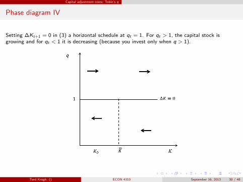
Phase diagram IV

Setting ∆Kt+1 = 0 in (3) a horizontal schedule at qt = 1. For qt > 1, the capital stock isgrowing and for qt < 1 it is decreasing (because you invest only when q > 1).


. . . . . .


Phase diagram V

Setting ∆qt+1 = 0 in (4) a downward sloping schedule for which (K , q) combinations that keepTobin’s q constant. For capital stocks to the left of the schedule the return to capital is high, sothe price today grows relative to the future price (i.e. ∆q < 0), so q is falling. To the right of theschedule the return on capital is so low that we need large capital gains to satisfy the optimalitycondition. q must grow.


. . . . . .


Phase diagram VI

This system features saddle-path stability: For a given K0 it is a unique level of q that puts thefirm on a path that converges at the steady state.


. . . . . .


Phase diagram VII

Starting from K0, the firms capital stock is low and its return to capital is high

Going straight to the steady state capital stock (as would have happened withoutadjustment costs) is too costly

From (2) it is clear that such a situation leads to a high (above 1) qt (and ∆qt+1 < 0) sincean extra unit of capital in this firm is valuable

The high shadow value stimulates investment, so K grows

As the capital stock is increasing, the shadow value falls, which then makes investment fall.In the end it converges to zero.

So having adjustment costs makes it possible to produce a more realistic investment response inwhich (i) the rate of investment is not infinite (even in continuous time), and (ii) that recognizesthat it takes time to adjust the capital stock.


. . . . . .


Phase diagram VIII

The unstable paths can be ruled out by assuming limT→∞(1 + r)−Tqt+T = 0. In addition theone going to the south-west quadrant gives q < 0 and K < 0 at some point – which is notpossible. Both paths are examples of bubbles; in the one case capital is increasing solely due toever-increasing beliefs of q, while the other represents ever-decreasing beliefs of q.


. . . . . .


Investment and the interest rate

What happened to the interest rate? Recall that we were discussing the relationship between theinterest rate and investment at the start of the lecture. We will now do three differentexperiments:

A permanent reduction in r from r0 to r1

A reduction in r believed to be permanent from r0 to r1 and then an increase to a levelbetween r1 and r0

An increase in r that is anticipated in advance


. . . . . .


Investment and the interest rate II

First experiment: A permanent reduction in the interest rate. This affects the ∆q = 0-locus.When the interest rate falls, a higher level of q is needed to keep ∆q = 0, so the curve shifts up.There is a new saddle path. A jump in q makes us move from the old steady state (A) to the newsaddle path (B). Will slowly converge to new steady state (C) with a higher capital stock.


. . . . . .


Investment and the interest rate III

Second experiment: The same reduction as in experiment 1. But when the firm has come topoint D, the interest rate is suddenly raised again to a level between the first and the second. Yetanother saddle path, and we jump from (D) to (E). For this interest rate the capital stock is toolarge, so we get a period of disinvestment until we converge at (F).


. . . . . .


Investment and the interest rate IV

Experiment 1 shows that the model retains the intuitively plausible mechanism that a lowerinterest rate leads to higher investment. Further, it leads to a higher value of the firm, whichis also intuitive.

However, as experiment 2 shows, the relationship between investment and the interest rate isstill far from as smooth as in the Keynesian investment function.

⇒ Point from Haavelmo still holds: There is no relationship between the rate of interest andthe rate of investment

We see that the movement from (E) to (F) gives disinvestment even though we can observepositive investment for a higher interest rate if we start out with K < K̄ .


. . . . . .


Investment and the interest rate V

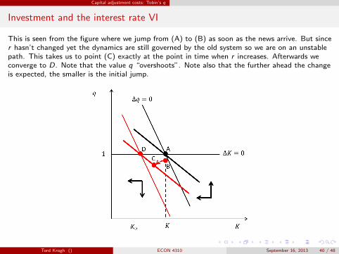
Third experiment: This time the firm anticipates a higher interest rate in the future. Whathappens? We know two things:

A higher interest rate gives a new ∆q = 0-locus and therefore also a new saddle path. Whenr changes, the new (K , q)-combination must be on the saddle path

But we also know that (in this case perfect foresight but more general) a forward lookingfirm will not wait until r changes: it is only with the arrival of news that q jumps

This means that q will jump before the interest rate moves. Then it will be on a smooth paththat ends up at the new saddle path exactly when r increases.


. . . . . .


Investment and the interest rate VI

This is seen from the figure where we jump from (A) to (B) as soon as the news arrive. But sincer hasn’t changed yet the dynamics are still governed by the old system so we are on an unstablepath. This takes us to point (C) exactly at the point in time when r increases. Afterwards weconverge to D. Note that the value q “overshoots”. Note also that the further ahead the changeis expected, the smaller is the initial jump.


. . . . . .

Tobin’s q and the stock-market value

Outline




...4 Summary


. . . . . .


Average and marginal q

qt is the shadow price of capital held at the end of period t in the firm, so qtKt+1 is anatural way to value the firm. But qt is unobservable.

We have already derived the value of the firm Vt as the NPV of future dividends from thefirm. This is presumably the stock-market value of the firm.

Is there a relation between qtKt+1 and Vt?


. . . . . .


Average and marginal q II

Assume first that there are no capital adjustment costs. Then qt = 1.

Since it is capital that makes up the firm, one should expect that the value of the firm equalsits capital stock Kt

But we also have that Vt equals the NPV of future dividends.

These valuations are consistent since:

AF (K , L) = AFKK + AFLL = rK + wL

(Euler’s theorem), so we can write dividends as:

ds = [rsKs + wsLs ]− wsLs − [Ks+1 − Ks ] = (1 + r)Ks − Ks+1

which makes the value of the firm:

Vt =∞∑

s=t+1

(1

1 + r

)s−t

[(1 + r)Ks − Ks+1] = Kt+1


. . . . . .


Average and marginal q III

Then we have adjustment costs. We start with (2):

qt =1

1 + r

(At+1FK (Kt+1, L̄) +

χ

2

(It+1

Kt+1

)2

+ qt+1

)

Multiply both sides by Kt+1 and use Kt+1 = Kt+2 − It+1 for the last term to the right:

qtKt+1 =1

1 + r

(At+1FK (Kt+1, L̄)Kt+1 +

χ

2

I 2t+1

Kt+1− qt+1It+1 + qt+1Kt+2

)

Insert for qt+1 = 1 + χ(It+1/Kt+1):

qtKt+1 =1

1 + r

(At+1FK (Kt+1, L̄)Kt+1 −

χ

2

I 2t+1

Kt+1− It+1 + qt+1Kt+2

)

Do a forward iteration and impose limT→∞(1 + r)−Tqt+TKt+T+1 = 0:

qtKt+1 =∞∑

s=t+1

(1

1 + r

)s−t (AsFK (Ks , L̄)Ks −

χ

2

I 2sKs

− Is

)


. . . . . .


Average and marginal q IV

Finally use that the production function is homogeneous of degree one so

AsFK (Ks , L̄) = AsF (Ks , L̄)− ws L̄

which means:

qtKt+1 =∞∑

s=t+1

(1

1 + r

)s−t (AsF (Ks , L̄)− ws L̄−

χ

2

I 2sKs

− Is

)= Vt

Perfect! So qtKt+1 equals the stock market value of the firm.


. . . . . .


Average and marginal q V

qt is often referred to as marginal q and is unobservable

Vt/Kt+1 is the average q and can be measured

But unfortunately only under a set of simplifying assumptions that average and marginal qcoincide (see Hayashi (1982)).


. . . . . .

Summary

Outline




...4 Summary


. . . . . .

Summary

Summary

Keynesian investment function I (r) is too naive

Simple neoclassical model shows that there is no simple relationship between investment andthe rate of investment

But the simple neoclassical model makes the capital stock adjust too quickly

Capital adjustment costs makes the response more realistic

But Haavelmo’s critique of the Keynesian investment function continues to hold

Tobin’s model not only makes investment more realistic: it also gives us a link betweeninvestment and the shadow value of capital in the firm q

Under simplifying assumptions, q can be identified from the stock market value per unit ofcapital


Investment: Tobin's q - Lecture 10, ECON 4310 Tobin’s q Lecture 10, ECON 4310 ... Today’s...

Documents

Transcript of Investment: Tobin's q - Lecture 10, ECON 4310 Tobin’s q Lecture 10, ECON 4310 ... Today’s...