Financial Fragmentation Despite Arbitrage

This Draft: October 2009

Preliminary

Stefan Klonner, Goethe University, Frankfurt

Ashok S. Rai, Williams College

Abstract: If there were no impediments to the �ow of capital across space, then the

returns to capital should be equalized. We provide evidence to the contrary. There are

large di¤erences in the return to comparable investments across di¤erent towns in the state

of Tamil Nadu in South India. We explore why these di¤erences are not arbitraged away

�and suggest that if one investor has monopoly power in arbitraging across towns then it

is in his pro�t-maximizing interest to reduce but not eliminate the di¤erences in returns to

capital.

JEL Codes: O16, G21

Keywords: credit constraints, limits to arbitrage

0We are grateful to the Chit Fund company (in South India) for sharing their data and their time.

And to Courtney Asher for research assistance. All errors are our own. Klonner: University of Frankfurt,

stefan@klonner.de; Rai: Dept. of Economics, Williams College, Williamstown, MA 01267, arai@williams.edu

1

1 Introduction

Many economists believe that �nancial market ine¢ ciencies are a cause of underdevelopment

and poverty (Aghion and Bolton, 1997; Banerjee and Newman, 1993; King and Levine, 1993;

Townsend 1997). There is a growing recent empirical literature documenting that capital

does not always �ow to its highest use. For instance, de Mel, Woodru¤ and Mckenzie

(2009) and Paulson,Townsend and Karaivanov (2006) �nd that �nance does not �ow to

high return entrepreneurs in Sri Lanka and Thailand respectively. Banerjee and Munshi

(2004) suggest that �nance does not �ow across ethnic lines in India. In the aggregate,

the misallocation of capital across �rms can explain low total factor productivity in Indian

and Chinese manufacturing (Banerjee and Du�o, 2005, Hsieh and Klenow, 2009).

In this paper we provide some striking evidence of �nancial market ine¢ ciencies across

space. We �nd large and signi�cant di¤erences in the returns to comparable �nancial

investments across local �nancial markets in the state of Tamil Nadu, India. The mean

rate annual rate of return ranges from 5:5 percent to 12:6 percent. If �nance �owed to its

highest use, such di¤erences would not exist.

The natural question then arises: If there is money to be made because of �nancial

fragmentation, is somebody doing it? We �nd that despite the presence of an investor who

arbitrages across locations these di¤erences in returns are not eliminated. We explore,

theoretically, how �nancial fragmentation may persist if there are barriers to entry into

arbitrage. The monopolist arbitrager in our setting makes pro�ts by preserving the spread

in returns at the expense of market e¢ ciency. Our �ndings contribute to the large literature

initiated by Shleifer and Vishny (1997) on the limits to arbitrage in �nancial markets. While

much of this literature studies how risk aversion, transaction costs or agency di¢ culties can

impede arbitrage, Borenstein et al (2008) explore a similar market power (cum transaction

costs for smaller traders) explanation for price di¤erences despite arbitrage opportunities

in California�s electricity market.

There is a related literature on di¤erences in US deposit and borrowing rates. In this

literature, several possible explanations for inter-regional interest rate di¤erences have been

2

advanced. Gendreau (1999) cites individuals� lack of access to national capital markets,

transaction costs, local monopoly power due to legal barriers, di¤erences in statuatory

interest rate ceilings and di¤erential borrower risk. Further, according to the same author,

di¤erences in bank risk may explain di¤erences in bank deposit rates. The institutional

setup we study allows us to exclude several of these factors as an explanation of di¤erences

in interest rates across space, namely local monopoly power due to legal barriers, di¤erences

in interest rate ceilings and di¤erences in bank risk. Furthermore, the data allows us to

evaluate the e¤ect of borrower risk as we have access to spatially disaggregated data on

borrower risk. The explanations for the di¤erences in interest rates that we observe then

are individual lack of access to national capital markets (or other forms of formal �nance

in our case) and transactions costs, which limit arbitrage possibilities.

The �nancial markets we study are organized through bidding Roscas (Rotating Savings

and Credit Associations). Roscas are �nancial institutions in which the accumulated savings

are rotated among participants (Anderson and Baland, 2003; Besley, Coate and Loury,

1994). The Roscas we study are anonymous and do not rely on internal social enforcement.

Since Rosca interest rates are determined by local auctions �and not set centrally as they

would be in a bank with several branches �this dataset provides an ideal opportunity to

investigate �nancial fragmentation. Further, unlike the anecdotal evidence summarized by

Banerjee and Du�o (2005) of di¤erences in risk-adjusted borrowing interest rates, we use

interest rates on local savings to measure fragmentation. The advantage of doing so is

that the savers in the bidding Roscas we study all face the same riskiness regardless of the

market in which they save �but adjusting for default risk or other unobservable loan terms

with borrowing interest rates is di¢ cult.

The paper proceeds as follows. In Section 2 we provide background on bidding Roscas

in South India and on our dataset. In Section 3 we outline some of the testable implications

from a simple model. We discuss our preliminary results in Section 4:

3

2 Institutional Background

This study uses data on Rotating Savings and Credit Associations (commonly referred to as

Roscas). Roscas match borrowers and savers but do so quite di¤erently from banks. They

are common in many parts of the world (Besley et al, 1993). In this section we provide

some background on how the Roscas in our study operate. We also describe the sample of

Rosca participants that we will use in our subsequent empirical analysis.

Rules

Roscas are �nancial institutions in which the accumulated savings are rotated among par-

ticipants. Participants in a Rosca meet at regular intervals, contribute into a "pot" and

rotate the accumulated contributions. So there are always as many Rosca members as

meetings. In random Roscas, the pot is allocated by lottery and in bidding Roscas the pot

is allocated by an auction at each meeting. Our study uses data on the latter.

More speci�cally, the bidding Roscas in our sample work as follows. Each month

participants contribute a �xed amount to a pot. They then bid to receive the pot in an

oral ascending bid auction where previous winners are not eligible to bid. The highest

bidder receives the pot of money less the winning bid and the winning bid is distributed

among all the members as an interest dividend. The winning bid can be thought of as the

price of capital. Consequently, higher winning bids mean higher interest payments. Over

time, the winning bid falls as the duration for which the loan is taken diminishes. In the

last month, there is no auction as only one Rosca participant is eligible to receive the pot.

We illustrate the rules with a numerical example:

Example (Bidding and Payo¤s) Consider a 3 person Rosca which meets once a month

and each participant contributes $10: The pot thus equals $30. Suppose the winning

bid is $12 in the �rst month. Each participant receives a dividend of $4: The recip-

ient of the �rst pot e¤ectively has a net gain of $12 (i.e. the pot less the bid plus the

dividend less the contribution, 30� 12 + 4� 10). Suppose that in the second month,

4

when there are 2 eligible bidders, the winning bid is $6: And in the �nal month,

there is only one eligible bidder and so the winning bid is zero: The net gains and

contributions are depicted as:

Month 1 2 3

Winning bid 12 6 0

First Recipient 12 -8 -10

Second Recipient -6 16 -10

Last Recipient -6 -8 20

The �rst recipient is a borrower: he receives $12 and repays $8 and $10 in subsequent

months, which implies a 30% monthly interest rate. The last recipient is a saver:

she saves $6 for 2 months and $8 for a month and receives $20, which implies a 28%

monthly rate. The intermediate recipient is partially a saver and partially a borrower.

The Sample

The bidding Roscas we study are large scale and organized commercially by a non-bank

�nancial �rm. The data we use is from the internal records of an established Rosca organizer

in the southern Indian state of Tamil Nadu.1 Our sample comprises Roscas that started

on or after January 1, 2002 and ended by November 2005: These Roscas took place in 78

branches of a non-bank �nancial �rm.

Our sample comprises 2170 Roscas of 34 di¤erent durations and contributions. The

most common Rosca denomination had 25 participants and a Rs. 400 monthly contribution

(with a total pot of Rs. 10; 000). There were also Roscas that met for longer durations (30

or 40 months) and with higher and lower monthly contributions. The average duration

of the Rosca in our sample was 29:55 months. These di¤erent Rosca denominations serve

1Bidding Roscas are a signi�cant source of �nance in South India, where they are called chit funds.

Deposits in regulated bidding Roscas were 12:5% of bank credit in the state of Tamil Nadu and 25% of bank

credit in the state of Kerala in the 1990s, and have been growing rapidly (Eeckhout and Munshi, 2004).

There is also a substantial unregulated chit fund sector.

5

to match borrowers and savers with di¤erent investment horizons. Descriptive statistics of

the Rosca denominations are in Table 1. Descriptive statistics at the Rosca level are in

Table 2.

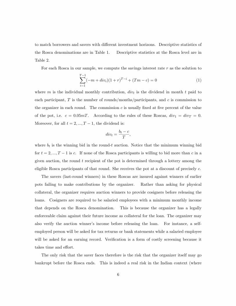
For each Rosca in our sample, we compute the savings interest rate r as the solution to

T�1Xi=1

(�m+ divi)(1 + r)T�i + (Tm� c) = 0 (1)

where m is the individual monthly contribution, divt is the dividend in month t paid to

each participant, T is the number of rounds/months/participants, and c is commission to

the organizer in each round. The commission c is usually �xed at �ve percent of the value

of the pot, i.e. c = 0:05mT . According to the rules of these Roscas, div1 = divT = 0.

Moreover, for all t = 2; :::; T � 1, the dividend is:

divt =bt � cT

;

where bt is the winning bid in the round-t auction. Notice that the minimum winning bid

for t = 2; :::; T � 1 is c. If none of the Rosca participants is willing to bid more than c in a

given auction, the round t recipient of the pot is determined through a lottery among the

eligible Rosca participants of that round. She receives the pot at a discount of precisely c.

The savers (last-round winners) in these Roscas are insured against winners of earlier

pots failing to make contributions by the organizer. Rather than asking for physical

collateral, the organizer requires auction winners to provide cosigners before releasing the

loans. Cosigners are required to be salaried employees with a minimum monthly income

that depends on the Rosca denomination. This is because the organizer has a legally

enforceable claim against their future income as collateral for the loan. The organizer may

also verify the auction winner�s income before releasing the loan. For instance, a self-

employed person will be asked for tax returns or bank statements while a salaried employee

will be asked for an earning record. Veri�cation is a form of costly screening because it

takes time and e¤ort.

The only risk that the saver faces therefore is the risk that the organizer itself may go

bankrupt before the Rosca ends. This is indeed a real risk in the Indian context (where

6

numerous chit fund companies have folded), but it is common to all the savers in all the 78

branches in the sample.

The average annual interest rate for a saver in these Rosca is 9.17 percent per year with

a standard deviation of 1.18 percent. At each location, interest rates are determined locally

through auctions. In contrast, the commercial bank savings rates are determined centrally

and are not based on local supply and demand for credit. So there is no variation. We

have obtained the rates on 3-6 month �xed deposits from the ICICI Bank, a large and well-

networked commercial bank, and those rates were at 6 percent or below for all of the study

period (2002-2005) with the exception of a six month period starting April 2002 when the

rate was 7.75 percent. The interest rates on commercial bank savings are substantially lower

than in the organized Rosca sector. This could re�ect a risk premium that the Rosca saver

must pay (since the organizer of the Roscas is more likely to go bankrupt than ICICI bank).

In addition, there is a uncertainty with the realized interest rate for a Rosca participant

(depending on the composition of the Rosca) that is absent in the commercial bank �xed

deposits.

Institutional Investors

In what follows we shall pay special attention to institutional investors who behave quite

di¤erently from other Rosca participants in the following ways. The institutional investors

operate in all 78 branches. They typically take several postions in Roscas in each branch.

These insitutional investors have close ties to the organizing company �and are not charged

a commission for participation (as a consequence, we will refer to them as "the company"

interchangeably in the sequel). Further, institutional investors are not considered default

risks and so they do not have to provide cosigners as collateral. Other participants, by

contrast, are location-speci�c, are charged a commission, and need to provide cosigners

when they win early pots.

7

3 A Model of Arbitrage in Roscas

In this section we consider a simple model of arbitrage between Roscas in two locations.

Our aim is to clarify how arbitrage can reduce reduce �nancial ine¢ ciencies but also to

point out the incompleteness of such arbitrage when there are barriers to entry.

Consider two spatially separated locations, each with n1 private agents. Each agent is

endowed with a dollar in the �rst period. Each agent has an investment opportunity with

a �xed investment cost of 2 at date 1 and yield 2p at date 2: Agents do not discount the

future. Agents vary in their productivity p. In each location, agents�types are distributed

according to Fi. Denote the corresponding mean by �i. Without loss of generality, we

assume �1 > �2, i.e. agents in location one are on average more productive than in location

2. We assume private information on individual types, i.e. each agent observes only her

own type and knows the distribution of types in her location.

In parts of the subsequent analysis, we employ the following additional assumptions:

A1 Fi is symmetric and unimodal

A2 F2 is a translation of F1, i.e. F2(p) = F1(p+ �1 � �2)

We model simple Roscas with two participants and hence two rounds. There is at

auction only at date 1: Each Rosca participant contributes a dollar at date 1 and the auction

is for the repayment amount b that is due at date 2: The winner of the auction receives the

pot and invests. There is a �xed commission of c charged for any net transfer in a Rosca.

As there are 2 net transfers in a Rosca, one in the �rst and one in the second period, the

total commission is 2c: We assume that each of the two participants pays a commission of

c when the Rosca is over (for simplicity, c is not part of the winning bid).2 So at date 2;2Remark: The idea why I use a commission of c and not 2c for the loan in the �rst round is that, in a

real Rosca with many members, the gross pot is mn and the gross transfer (gross of the bid) from the n� 1

lenders to the borrower is (n � 1)m: The total commission in that round is nmc. So the commission per

dollar transacted is nmc=(n � 1)m � c. On the other hand, when n is only two, as in the model, and we

applied the actual Shriram commission rule, we would have a commission of 2c per dollar transacted, which

is too much compared to the real Roscas.

8

the winner pays b to the loser of the �rst-round auction and c to the organizer. The loser

of the �rst-round auction receives b from the winner and also pays c to the organizer. (In

this way, we model how Rosca auctions determine the interest rate but abstract from the

speci�c rules that are used in practice in the Roscas in our sample).

No Arbitrage

We �rst show that the interest rate di¤erence across locations is given by di¤erences in

average productivity, �1 � �2, in the absence of arbitrage. More formally, an agent�s

willingness to pay is found by equalizing her payo¤ from winning, 2p� b; to her payo¤ from

losing, b; which gives

b� = p:

In a Rosca, two individuals of a location are randomly matched. In each Rosca, each

participant is uninformed about the other participant�s type, and hence willingness to pay.

We are thus in a situation of an symmetric, independent, private-value auction. Since the

Roscas we consider have open-ascending bid auctions, the appropriate bidding equilibrium

is most easily found by modelling the auction as a second-price sealed bid auction, which

is payo¤-equivalent. It can be shown that, in such an auction, each bidder determines her

bid by a strictly increasing function hi(p), where hi(p) � p for all p, hence there is some

overbidding relative to one�s valuation of the pot. The di¤erence in interest rates between

branches, or spread for short, is

�r = E[h1(P2:2)� h2(P2:2)]:

Under assumption A2, we have that h2(p) = h1(p)� (�1��2): Denoting �1��2 by �� we

then have that

�r = ��

9

Monopolistic Arbitrage, No entry

We next consider the case where the Rosca organizer can arbitrage across locations and has

monopoly power. We �nd that interest rate di¤erences persist but they are smaller than

inter-locational di¤erences in average productivity, �1��2. The arbitrager will borrow in

the low interest rate location and save in the high interest rate location �while preserving

the spread in order to make pro�ts.

The Rosca company has the choice to become a Rosca member herself in each of the two

locations at no cost. We assume that the company�s agent enters a Rosca with a private

agent. We assume that the private agent knows of his co-participant�s identity and that

the company�s agent plays a pure strategy in each location, i.e. she bids bi in all Roscas

in location i where the company becomes a member. When the private agent in location

i knows the company-agent�s bi, he will bid bi minus an increment whenever p < bi and bi

plus an increment when p > bi. In both of these cases, the auction price will be roughly bi.

If the company holds one ticket in each of the branches, its expected pro�t is

� = b1(1� F1(b1)) + b2(1� F2(b2))� [b1F1(b1) + b2F2(b2)] (2)

Notice that (1�F1(b1)) is the expected number of period 1 pots that the company loses in

location 1, F1(b1) is the number of period 1 pots the company wins in location 1, each of

which generates a liability of b1 in the second period. Hence b1(1�F1(b1)) is the company�s

expected income in the second period from the lost auctions in location 1 and b1F1(b1) the

liability from the won auctions in location 1.

To balance the budget in period one (in expectation), the company cannot lose more

period 1 pots than it wins,

F1(b1) + F2(b2) � (1� F1(b1)) + (1� F2(b2)) (3)

The company maximizes its pro�ts by choice of b1 and b2 subject to (3).

Lemma 1 A strictly positive pro�t of the company implies that she chooses bids such that

�1 > b1 > b2 > �2; (4)

10

which implies that the di¤erence in interest rates is smaller than the di¤erence in

average productivity,

�r < ��:

Proof: It is convenient to rewrite the company�s pro�t as

� = b1(1� 2F1(b1)) + b2(1� 2F2(b2)) (5)

and the budget-balance constraint as

F1(b1) + F2(b2) � 1 (6)

We �rst proof �1 > b1. To this end, suppose b1 � �1. This implies. We take each of the

following two cases in turn, (i) b2 � �2 and (ii) b2 > �2: Under (i) 1�2F1(b1) � 0 and

1�2F2(b2) � 0, which implies � � 0. This contradicts � > 0. Under (ii) 1�2F1(b1) �

0; 1� 2F2(b2) > 0, b2 > b1 and (6) implies that 1� 2F2(b2) � �(1� 2F1(b1)). So we

can write

� � b1 [(1� 2F1(b1)) + (1� 2F2(b2))] � b1 [(1� 2F1(b1))� (1� 2F2(b2))] = 0

Second we proof that b2 > �2. To this end, suppose b2 � �2. Based on the previous

result, it is su¢ cient to consider b1 < �1. In this case F1(b1) < 1=2 and F2(b2) � 1=2,

which implies that F1(b1) + F2(b2) < 1. This contradicts (6).

Next we proof that b1 > b2. To this end suppose that b1 � b2 and employ �1 > b1,

which implies F1(b1) < 1=2 and 1� 2F1(b1) > 0; and b2 > �2, which implies F2(b2) >

1=2 and 1� 2F2(b2) < 0. We may now write

� � b2 [(1� 2F1(b1)) + (1� 2F2(b2))] � 2b2 [1� (F1(b1)� F2(b2))] = 0

where the last inequality follows from (6). But this contradicts � > 0: �

This lemma shows that (a) interest rates will vary across locations and (b) arbitrager�s

rank is positively correlated with the interest rate and (c) if the constraint (6) is binding -

that the average rank of the arbitrager is 0.5. The positive correlation between the local

11

interest rate and the arbitrager�s rank follows from �1 > b1; which implies F1(b1) < 1=2;

and b2 > �2, which implies F2(b2) > 1=2: In other words, across locations, the arbitrager is

less likely to win the �rst pot, the higher b:

The following example illustrates the result:.

Example with Uniform Distributions We consider uniform speci�cations of F1 and

F2 with an identical range of �,

Fi(b) =(b� �i)�

+1

2; �i �

�

2� b � �i +

�

2:

We will assume that the two distributions overlap su¢ ciently, speci�cally

�1 � �2 � 2�:

Notice that, for an e¢ cient allocation of funds in this economy (which in the current

setup implies an identical price of credit in the two locations), an amount of �1 �

�=2� (�2 � �=2) = �1 � �2 per private customer in location i (or n1 [�1�2] in total)

would have to be transferred by the arbitrager from location 2 to location 1 in period

1.

De�ne

gi(b) = b+Fi(b)� 1

2

fi(b):

In general, the solution to the company�s problem of maximizing (5) by choice of b1

and b2 subject to (6) can be charcterized by the two equations

g1(b1) = g2(b2); (7)

F1(b1) + F2(b2) = 1: (8)

For the uniform distributions considered here, this gives

b1 = �1 ��1 � �24

; b2 = �2 +�1 � �24

:

The average rank of the company in the strong and weak location are

1

2+��4�

and1

2� ��4�;

12

respectively.

Thus, through the activity of the arbitrager, the interest rate di¤erence is half the

average productivity di¤erence,

�r =1

2��:

The amount which is transferred from location 2 to 1 in the �rst period is ��=2. This

is just half of the amount that would be transferred in an e¢ cient allocation of funds

across the two locations.

The company�s pro�t is

�A =(�1 � �2)2

4�:

Monopolistic Arbitrage, Free Entry

If there is free-entry into arbitrage then the interest rate di¤erences disappear. Suppose

the organizer bids any pair (b1; b2), satisfying �2 � b2 < b1 � �1. Then an entrant can

become a Rosca member in the two locations, bid b2 plus an increment in location 2 and b1

minus an increment in location 1. The entrant will win for sure in location 2 at a price of b2

and lose for sure at a price of b1 in location 1. This will yield the entrant a positive pro�t of

b1� b2. When enough such entrants are active, the organizer�s pro�ts will become negative

because now the company wins too many auctions in location 1 and loses too many in 2.

The only equilibrium involves b1 = b2, i.e. � = 0; and zero pro�ts for the organizer. (Note

that if the two locations had access to a common �nancial market, i.e. were integrated, then

too such interest rate di¤erences would disappear).

Monopolisitic Arbitrage, Costly Entry

We consider the �nal case where the Rosca organizer can arbitrage costlessly but entrants

to arbitrage must pay the cost c of Rosca membership. We �nd that the di¤erences in

interest rates persist but are smaller smaller than the no-entry case when the di¤erence in

productivity is su¢ ciently large relative to the cost of entry (�1 � �2 > 2c), and equal to

13

the no-entry case when the producitivity di¤erence is not su¢ ciently large (�1 � �2 � 2c):

More speci�cally, the di¤erence in interest rates is capped by max(�1 � �2; 2c):

Suppose the company bids any pair (b1; b2), satisfying �2 � b2 < b1 � �1. Then

an entrant can become a Rosca member in the two locations, bid b2 plus an increment in

location 2 and b1 minus an increment in location 1. The entrant will win for sure in location

2 at a price of b2 and lose for sure at a price of b1 in location 1. But now he faces a total

cost for the two memberships of 2c. So the entrant will make a pro�t of b1 � b2 � 2c. This

is positive only when b1 � b2 � 2c. As a consequence, the company cannot sustain a higher

spread than 2c in equilibrium. When c is su¢ ciently large - relative to the di¤erence in

average productivity -, there will be no entrants and the outcome will be the same as with

monopolistic arbitrage and no entry.

We turn to the question of why arbitrage by outsiders (i.e. not the Rosca organizer)

may be costly in practice. First, the cost of arbitrage predicted by our model due to the

commission charged by the company will in practice equal 10% between the �rst and last

round. For the sample Roscas, this amounts to comparing the interest rate over the entire

duration of a Rosca which is on average 30 months. So a necessary condition for an outsider

arbitrageur to make non-negative pro�ts will be that the interst rate spread in months

between two locations where she participates is at least (roughly) 10=30 = 0:33%. There are,

however, two additional factors that complicate arbitrage by an entrant. First, whenever

the arbitrageur obtains an early pot she has to provide cosigners, which may cause a (non-

monetary) additional cost. Second, the arbitrageur faces uncertainty as he has to subscribe

to Roscas in certain branches upfront, i.e. when Roscas start. If locations experience

productivity shocks while Roscas are going on, however, the interest rate di¤erence between

two locations with an initially large spread may shrink and render the arbitrageur�s pro�ts

negative. To summarize this point, in our institutional setup we would expect only limited

scope for outside arbitrageurs unless interest rate di¤erences between locations substantially

exceed 0.33% per month for the majority of pairs of branches.

14

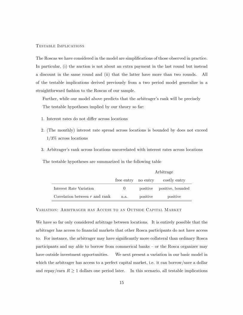
Testable Implications

The Roscas we have considered in the model are simpli�cations of those observed in practice.

In particular, (i) the auction is not about an extra payment in the last round but instead

a discount in the same round and (ii) that the latter have more than two rounds. All

of the testable implications derived previously from a two period model generalize in a

straightforward fashion to the Roscas of our sample.

Further, while our model above predicts that the arbitrager�s rank will be precisely

The testable hypotheses implied by our theory so far:

1. Interest rates do not di¤er across locations

2. (The monthly) interest rate spread across locations is bounded by does not exceed

1=3% across locations

3. Arbitrager�s rank across locations uncorrelated with interest rates across locations

The testable hypotheses are summarized in the following table

Arbitrage

free entry no entry costly entry

Interest Rate Variation 0 positive positive, bounded

Correlation between r and rank n.a. positive positive

Variation: Arbitrager has Access to an Outside Capital Market

We have so far only considered arbitrage between locations. It is entirely possible that the

arbitrager has access to �nancial markets that other Rosca participants do not have access

to. For instance, the arbitrager may have signi�cantly more collateral than ordinary Rosca

participants and my able to borrow from commerical banks �or the Rosca organizer may

have outside investment opportunities. We next present a variation in our basic model in

which the arbitrager has access to a perfect capital market, i.e. it can borrow/save a dollar

and repay/earn R � 1 dollars one period later. In this scenario, all testable implications

15

continue to hold except for the company�s average rank, which may now be greater or

smaller than one half (depending on whether R is closer to �1 or �2).

Suppose now that the company has access to a perfect capital market, i.e. it can

borrow/save a dollar and repay/earn R � 1 dollars one period later. In this situation, the

company arbitrages not only between branches, but also between Roscas in general and the

capital market.

The company�s maximization problem (5) subject to (6) now becomes (the uncon-

strained problem)

maxb1;b2

(b1 �R)(1� 2F1(b1)) + (b2 �R)(1� 2F2(b2)):

Notice that the term bi � R is the period two pro�t for each pot won in location i. The

solution can be characterized by the two equations

g1(b1) = g2(b2) = R: (9)

Notice that the �rst equality is the same as in the situation of pure arbitrage; see (7). It

hence follows that for an appropriate value of R, R0 say, the two scenarios yield the same

values of b1 and b2, and hence identical testable implications. However, in general the

previously derived implication "company�s average rank equals one half" will not continue

to hold (whenever R 6= R0). Denoting the company�s average rank by rk 2 [0; 1] (i.e. 0 for

winning early and 1 one for winning late pots only), recall that

rk = 1� F1(b1) + F2(b2)2

:

One can derive the comparative static result,

d rk

dR= �1

2

�f1(b1)

g01(b1)+f2(b2)

g02(b2)

�:

As g0i(bi) will usually be positive (a su¢ cient condition is A1), this multiplier will usually

be negative. This is as expected: the higher the interest rate in the capital market, the

more likely is the company to be a net borrower in Roscas.

16

Example with Uniform Distributions

We consider the same uniform speci�cations of F1 and F2 as in the previous example.

The conditions (9) imply that

bi =R+ �i2

;

i.e. the company�s bid is simply the average of the capital market interest rate and

the average productivity in location i. As a consequence,

�r =1

2��;

i.e. the interest rate spread accross branches is precisely the same as with pure mo-

nopolistic arbitrage. So, at least in this example, access to a perfect capital market

does not a¤ect sptatial price fragmentation in Roscas.

The average rank of the company is now

rk =1

2

�1 +

�R� �1 + �2

2

��;

i.e. for R = (�1 + �2)=2, the rank is precisely one half (as with pure arbitrage), while

a larger R implies a higher (=later) average rank of the company.

For the company�s pro�ts, we have

�CM =(�1 �R)2 + (�2 �R)2

2�:

It can be shown that �CM = �A i¤R = (�1+�2)=2 and �CM > �A i¤R 6= (�1+�2)=2

(more precisely, �CM is convex in R and has its minimum at R = (�1+�2)=2). So the

company will in generally be better o¤ when it can combine inter-locational arbitrage

with arbitraging between Roscas and the capital market more broadly.

4 Results

Financial Fragmentation

We �rst explore the extent of fragmentation of interest rates accross space. Towards this

we estimate

17

rdij = ai + udij

by OLS, where d indexes denominations, i branches, and j Rosca groups of denomination d

in branch i. The interest rate r is computed for each Rosca in our sample according to (1).

The resulting branch means bai are plotted in �gure 1, where a numerical branch identi�eris on the horizontal axis, and the (monthly) implied interest rate on the the vertical axis.

Figure 2 maps branch interest rates. Statistics of the distribution of the bai�s are set out inTable 3, column 1. Accordingly, the coe¢ cient of variation is 0.099/0.76 = 0.13 and the

hypothesis of equality of all ai�s is rejected at the 1% level.

Now we will control for the denomination of a Rosca and the date when a Rosca takes

place. This is important because a Rosca of a di¤erent denomination is a di¤erent �nancial

product and the portfolio of Rosca denominations varies over branches. Moreover, even

when there is no di¤erence in interest rates over locations at any given point in time, this

interest rate may vary over time. Therefore we also control for the date at which a Rosca

was started. Our sample Roscas were started between January 2001 and October 2003.

We denote by quarterkdij a dummy variable which is equal to one for all Roscas that were

started in quarter k 2 f1; :::; 12g; where k = 1 covers the three months spell Januar to

March 2001, and zero otherwise. We estimate

rdij = �i + d +

12Xk=2

quarterkdij + udij : (10)

Rather than reporting the point estimates of this regression, column 2 of table 3 reports

the properties of the estimated branch intercepts. Accordingly, the standard deviation is

reduced by only about 4 percent, from 0,099 to 0.095. The hypothesis of equal interest rates

accross branches is still clearly rejected. From this exercise, we conclude that the bulk of

spatial variation fails to be explained by di¤erences in Rosca denominations or Rosca dates.

It is also interesting to note that the correlation beteween the estimated branch interecepts

in columns 1 and 2 is 0.96.

18

Further Sources of Fragmentation: Borrower Risk, Collateral Require-

ments and Screening

The interest rate which we is used as the dependent variable in the previous estimations

is a pure savings rate. However, de facto it is an increasing function in the winning bids

of each rounds from 2 to n � 1 in the Rosca. Hence it is also a kind of average of the

price of funds implicit in all loans made over the course of a Rosca. An important question

hence is whether spatial di¤erences in our interest rates are due to fundamentally di¤erent

borrowing conditions in local credit markets. We capture risk-characteristics of loans by

the default rate, the number of cosigners required on a loan and the screening e¤ort of

the lender. The latter is captured by an indicator which equals one if the Rosca company

veri�ed occupation and income of a borrower, and zero otherwise. Descriptive statistics of

these three variables at the Rosca level are set out in table 2. Accordingly, 4.78% of dues

have not been repaid by the time a Rosca ends, the company requires an average of 1.1

cosigners per loan and veri�es the borrower�s income 44% of the time.

As we are particularly interested in explaining spatial variation in interest rates, we

will not simply add realizations of the variables to estimation equation (10), where each

observation is one Rosca. Instead, we �rst estimate equation (10) with each of the three

risk measures as left hand side variable in turn. This yields branch means net of time

and denomination e¤ects. In a second step, we use these estimated branch �xed e¤ects as

explanatory variables in a regression with the estimated interest-rate branch intercepts from

equation (10) as the left and side variable. This latter regression thus has 78 observations,

one for each branch.

To start out, in table 4 we have set out some descriptive statistics of the estimated

branch �xed e¤ects of three regressions (10) with default rate, number of cosigners, and

income veri�cation as the left hand side variable, respectively. According to the resulting

coe¢ cients of variation, these risk measures exhibit substantially greater spatial variation

than the interest rate (where the CV is 0.13).

Column 1 of table 5 summarizes the results of a linear regression speci�cation of the

19

interest rate branch �xed e¤ects on the estimated �xed e¤ects of the three risk variables.

Column 2 adds squared terms of the explanatory variables. According to the results, only

defaults are signi�cantly correlated with interest rates, where - as expected in e.g. a Stiglitz-

Weiss world - riskier borrowers have a higher willingness to pay for loans. Column 3 of

table 3 summarizes the distribution of the residuals from this regression. Accordingly, the

standard deviation is reduced goes down to 0.080 after controlling for the risk factors. The

null hypothesis of complete market integration fails to be rejected, however.

The lower panel of that table gives p-values of tests for equal variances between pairs of

the three samples of estimated �xed e¤ects (or residuals in the case of column 3). While the

di¤erence between the �rst and the second, and the second and third speci�cations are zero,

there is, at least at the 10 percent level, a signi�cant reduction in fragmentation between

the �rst and third speci�cation. Thus risk together with controls for denomination and time

signi�cantly explain about 20 percent of spatial di¤erences in interest rates as measured by

the standard deviation. The remaining 80% remain unexplained, however.

Arbitrage

We next test if there is systematic arbitrage between locations by the company: We measure

the rank (or position) of the winner of a pot on a 0 to 1 scale, where 0 represents a receipt

of the �rst pot �and 1 represents the receipt of the last pot. More preciselz, we de�ne the

rank of the winner of the t�th pot in the j�th Rosca of denomination d in location i as

rankdijt =t� 1Td � 1

;

where Td denotes the duration (in months) of denomination d. Descriptive statistics on the

company�s participation at the Rosca level are set out in table 2. Accordingly, the company

holds about a third of all Rosca memberships and on average occupies a rank of 0.41, which

indicates that the company on average wins pots earlier than in the middle of a Rosca. These

same variables at the branch level are set out in table 4. According to the coe¢ cient of

variation, the company�s activities exhibits spatial variation on a similar order of magnitude

20

as the interest rate. The mean rank of the company of .41 indicates that the company is

more interested in early than in late pots, and thus, within our theoretical framework, might

be arbitraging not only across branches but also against an outside investment opportunity

with a higher rate of return than the average in the Roscas. In all but three of the 77

branches, the institutional investor�s rank is below 0:5:

Pro�t maximizing arbitrage by the company (which reduces spatial variation in interest

rates without eliminating them) implies a positive correlation between the local interest rate

and the company�s rank in the respective location. Using only pots won by the company,

we �rst estimate

rankdijt = bi + d +12Xk=2

quarterkdij + vdijt;

where t indexes the round in a Rosca, t = 2; :::; Td. Figure 3 plots the resulting branch

�xed e¤ects bbi on the vertical axis against the estimated �xed e¤ects of (10) in its originalversion (with the interest rate as the dependent variable) on the horizontal axis. Clearly,

there is a positive relationship between these two variables. Hence,the institutional investor

takes relatively early pots (i.e. borrows) where interest rates are relatively low, and waits

to take later pots when interest rates are relatively high. We can also formally reject the

null hypothesis of no arbitrage by the company: the correlation coe¢ cient between the two

variables is 0.48 and signi�cantly bigger than zero at the one percent level.

As pointed out in the theory section, costless competitive arbitrage would result in a

uniform interest rate across locations. The company for whom arbitrage is fairly costless,

or at least relatively cheap (as it neither has to pay the 5% participation fee nor provide

cosigners at the time of borrowing), has to be regarded as a monopolistic arbitrager, how-

ever. In this paragraph, we brie�y discuss how the observed interest rate heterogeneity

across space largely conforms with the institutional feature of a substantial cost of arbi-

trage for outsiders. According to the theory, competitive costly arbitrage will drive down

the interest wedge between any two locations to twice the entry fee. As our sample Roscas

have a duration of more than two months, this fee has to be scaled to a fee per month to

make it comparable to the monthly interest rates. Accordingly, the fee amounts to roughly

21

0.33% per month (two times 5% divided by the average Rosca duration of 30 months).

Thus an interest di¤erence of 0.33% between any two branches is largely in accordance

with competitive, albeit costly, arbitrage in this institutional setup. According to table 3,

column 1, the range of interest rates is larger than that, 0.505. However, when we consider

all possible pairs of branches, 97% percent of pairs have a di¤erence not exceeding 0.33.

Considering, �rst, that the entry fee is not the only cost for an outside arbitrager - he also

has to provide collateral for loans and employ agents in di¤erent locations - and, second,

that local interest rates may also be subject to idiosyncratic shocks which are not perfectly

predictable (and an outside aribtrager will su¤er a loss for any pair of locations where the

interest di¤erence is less than his cost), the spatial distribution of interest rates appears to

be largely in accordance with a scenario of monopolistic arbitrage with costly entry, where

the cost is about as large as the entry fee.

5 Conclusion

The principle of no-arbitrage, so crucial to economic reasoning, implies that risk-adjusted

interest rates should be equalized across �nancial markets. We have presented evidence to

the contrary. The �nancial markets we study are those organized in di¤erent towns in the

South Indian state of Tamil Nadu. The interest rates we analyze are determined by local

auctions. These interest rates accrue to savers who face an identical risk across markets.

What is remarkable about this variation in interest rates is that it persists despite the

presence of an arbitrager who borrows in low-interest locations and saves in high-interest

locations. We provide an explanation for why this arbitrager may deliberately choose to

maintain the interest rate spread at the cost of �nancial e¢ ciency and discuss entry barriers

into arbitrage that enable such monopoly pro�ts.

Our results raise questions about the competition between the organized (and regulated)

Roscas in our study and the commercial banking sector. One might expect then that the

variation in interest rates between �nancial markets may depend partly on the presence of

bank branches in those locations. In ongoing research we are studying whether the presence

22

of bank branches reduces the �nancial ine¢ ciencies across markets. Relatedly, it would be

useful to understand if the liberalization of the Indian economy in the 1990s has promoted

more e¢ cient �ow of �nance across markets. By historically studying the evolution of

interest rates across Rosca locations we hope to provide an insight into this question.

References

[1] Aghion, P. and P. Bolton, 1997. A Theory of Trickle-Down Growth and Development.

Review of Economic Studies, 64(2): 151�172.

[2] Anderson, S. and J. Baland, 2002: The Economics of Roscas and Intrahousehold

Resource Allocation, Quarterly Journal of Economics, 117(3); 963� 995.

[3] Banerjee, A. and A. Newman, 1993, Occupational Choice and the Process of Develop-

ment. Journal of Political Economy, 101: 274�298.

[4] Banerjee, A. and K. Munshi. 2004: How E¢ ciently is Capital Allocated? Evidence

from the Knitted Garment Industry in Tirupur.�Review of Economic Studies 71(1):19-

42.

[5] Banerjee, Abhijit and Esther Du�o (2005), �Growth Theory Through the Lens of

Development Economics,� chapter 7 in the Handbook of Economic Growth Vol. 1A,

P.Aghion and S. Durlauf, eds., North Holland.

[6] Besley, T., S. Coate and G. Loury. 1994: Rotating Savings and Credit Associations,

Credit Markets and E¢ ciency. The Review of Economic Studies, 61(4): 701-719

[7] Borenstein, Severin, Knittel, Christopher R. and Wolfram, Catherine D., 2008. Ine¢ -

ciencies and Market Power in Financial Arbitrage: A Study of California�s Electricity

Markets. The Journal of Industrial Economics, Vol. 56, Issue 2, pp. 347-378.

[8] de Mel, S., Mckenzie, D. and C. Woodru¤, Returns to Capital in Microenterprises:

Evidence from a Field Experiment. forthcoming, Quarterly Journal of Economics.

23

[9] Klenow, P. and C-T Hsieh, forthcoming "Misallocation and Manufacturing TFP in

China and India" Quarterly Journal of Economics

[10] Eeckhout, J. and K. Munshi, 2004: Economic Institutions as Matching Markets. Man-

uscript, Brown University.

[11] King, R. G, and R. Levine, 1993. Finance and Growth: Schumpeter Might be Right.

Quarterly Journal of Economics, 108(3): 717�737.

[12] Paulson, Anna L., Robert Townsend and Alex Karaivanov 2006: Distinguishing Limited

Liability from Moral Hazard in a Model of Entrepreneurship," Journal of Political

Economy Vol. 114. No. 1, pp. 100 -144

[13] Shleifer, A. and R. Vishny 1997. The Limits to Arbitrage. Journal of Finance, 52:1,

35-55.

[14] Townsend, R. 1997: �Microenterprise and Macropolicy�in Kreps, D. and K. Wallis eds.

Advances in Economics and Econometrics: Theory and Applications, Seventh World

Congress of the Econometric Society, Cambridge University Press, II:160-209.

24

Table 1. Descriptive Statistics, Rosca DenominationsDuration (Months)

Contribution (Rs./month)

Pot (Rs.) FrequencyRelative 

Frequency25 400 10,000 488 23.7425 600 15,000 8 0.3925 800 20,000 9 0.4425 1,000 25,000 278 13.5225 2,000 50,000 214 10.4125 4,000 100,000 80 3.8925 8,000 200,000 2 0.1025 12,000 300,000 1 0.0525 20,000 500,000 3 0.1530 500 15,000 282 13.7230 1,000 30,000 98 4.7730 1,500 45,000 2 0.1030 2,000 60,000 22 1.0730 2,500 75,000 11 0.5430 3,000 90,000 7 0.3430 4,000 120,000 1 0.0530 5,000 150,000 53 2.5830 10,000 300,000 22 1.0730 20,000 600,000 4 0.1930 25,000 750,000 1 0.0530 30,000 900,000 2 0.1040 250 10,000 176 8.5640 375 15,000 1 0.0540 500 20,000 3 0.1540 625 25,000 85 4.1340 750 30,000 2 0.1040 1,250 50,000 77 3.7540 1,500 60,000 3 0.1540 2,500 100,000 99 4.8240 3,750 150,000 2 0.1040 5,000 200,000 4 0.1940 7,500 300,000 4 0.1940 12,500 500,000 4 0.1940 12,500 500,000 3 0.1540 15,000 600,000 1 0.0540 25,000 1,000,000 4 0.19

Table 2. Descriptive Statistics, Sample RoscasMean Std. Dev. Minimum Maximum

Duration (months) 29.64 5.99 25.00 40.00Contribution (Rs./month) 1,468.12 2,462.76 250.00 30,000.00Pot (Rs.) 44,277.72 81,223.17 10,000.00 1,000,000.00Date of first auction August 30, 2002 181 (days) Jan 2, 2002 Sept 13, 2003Monthly Interest Rate (%) 0.74 0.22 0.00 1.59Default Rate (%) 4.78 2.55 0.00 19.68Cosigners 1.10 0.62 0.00 3.89Income Verification 0.44 0.25 0.00 0.97Company Participation 0.32 0.19 0.00 0.95Company Rank 0.41 0.10 0.08 0.83

Number of observations: 2,056

Table 3. Monthly savings rates, summary of estimated fixed effects/residuals

Without Controls With Controls Net of Defaults,(time, denomination) collateral, screening

(1) (2) (3)Mean 0.760Standard Dev. 0.099 0.095 0.080Range 0.505 0.475 0.463Test for Equality (p) 0.000 0.000 0.000

Test for Equal Variances (p‐value):       (1) and (2) 0.716       (1) and (3) 0.069       (2) and (3) 0.147

Number of observations: 78

Table 4. Distribution of Estimated Fixed Effects of other VariablesMean Range Std Coeff. of Var.

Default Rate (%) 4.185 6.839 1.374 0.328Cosigners 1.140 2.224 0.421 0.369Income Verification 0.455 0.758 0.191 0.420Company Participation 0.343 0.331 0.078 0.228Company Rank 0.410 0.202 0.043 0.105

Notes:The mean is the average over all Roscas in the sampleRange and standard deviation are calculated from estimated branch fixed effectsCV is the standard deviation divided by the mean as reported in this table

Table 5. Explaining Spatial Interest Rate DifferencesDependent Variable: Branch intercepts from interest rate regression

(1) (2)Intercept 0.666 *** 0.805 ***

(0.045) (0.093)Defaults 0.028 *** ‐0.042

(0.007) (0.030)Defauts Squared 0.009 **

(0.004)Cosigners 0.034 ‐0.003

(0.023) (0.131)Cosigners Squared 0.016

(0.045)Screening ‐0.083 ‐0.122

(0.052) (0.359)Screening Squared 0.036

(0.313)

R‐Squared 0.23 0.24Number of observations 78 78

Notes:all explanatory variables are estimated branch fixed effects from a regression of the explanatory variable on branch FEs denomination and time dummies

Figure 1. Distribution of Branch Interest Rates

Figure 2. Map of Branch Interest Rates

Figure 3. Scatter Plot of Company's Rank and Local Interest Rates