
THE EMPIRICAL FOUNDATIONS OF ARBITRAGE...
42
Jouxnal of Fhmtial Economics ‘?I (3958) 213-254. North-Holland THE EMPIRICAL FOUNDATIONSOF THE ARBITRAGE PRICING THEORY* David ha. MODEST Received 0ctober 1985, &nal version received January 1988 The arbitrage pricing theory (APT) developed by Ross (1976,1977) is a major attempt to overcome the problems with testzbility’ and anomalous euqkical evidence that have plagued the static and iktertemporal capital asset pricing models (CAPMs). The main assumption of the theory is that the returns of a large (in the limit infinite) number of assets can be broken into two components: nondiver&able, systematic rislc,which can be measured as exposure to a small number of common factors, and idiosyncratic risk, which *We are grateful to the Faculty Research Fund of the Columbia Business School and i&z Institute for Quantitative Research iz Finance for their support and to Wayne Ferson and Allan Kleidon for comments on earlier drafts. We owe a special debt of gratitude to Jay Shauken (the refer) for signikantly improving the paper through his incisive comments and for pointing out severai errors in earlier drafts. The usual disclaimer applies. ‘The model does not resolve all empirical ambiguities of the type discuss4 in Roll (1977). Jtn particular, !Shanken (1982,198Sa) has emphasized that the absence of riskless arbitrage opportuni- ties coupled with the linear factor model for security returns does not place sufficiently precise restrictions on expected returns. In section 2 we address this i$nt further and sqecify a set of additional assumptions, that is sufficient to perform preci§e statistical tests. 0304405X/88,/,93.50 0 1,988, Ekevier Science Publishers B.V. (North-
Transcript of THE EMPIRICAL FOUNDATIONS OF ARBITRAGE...

Jouxnal of Fhmtial Economics ‘?I (3958) 213-254. North-Holland
THE EMPIRICAL FOUNDATIONS OF THE ARBITRAGE PRICING THEORY*
David ha. MODEST
Received 0ctober 1985, &nal version received January 1988
The arbitrage pricing theory (APT) developed by Ross (1976,1977) is a major attempt to overcome the problems with testzbility’ and anomalous euqkical evidence that have plagued the static and iktertemporal capital asset pricing models (CAPMs). The main assumption of the theory is that the returns of a large (in the limit infinite) number of assets can be broken into two components: nondiver&able, systematic rislc, which can be measured as exposure to a small number of common factors, and idiosyncratic risk, which
*We are grateful to the Faculty Research Fund of the Columbia Business School and i&z Institute for Quantitative Research iz Finance for their support and to Wayne Ferson and Allan Kleidon for comments on earlier drafts. We owe a special debt of gratitude to Jay Shauken (the refer) for signikantly improving the paper through his incisive comments and for pointing out severai errors in earlier drafts. The usual disclaimer applies.
‘The model does not resolve all empirical ambiguities of the type discuss4 in Roll (1977). Jtn particular, !Shanken (1982,198Sa) has emphasized that the absence of riskless arbitrage opportuni- ties coupled with the linear factor model for security returns does not place sufficiently precise restrictions on expected returns. In section 2 we address this i$nt further and sqecify a set of additional assumptions, that is sufficient to perform preci§e statistical tests.
0304405X/88,/,93.50 0 1,988, Ekevier Science Publishers B.V. (North-

214 B.N Lehmann and D. M. Modest, Empirical basis of the a&rage pricing theory
em be eliminated in large weW.iversified portfolios. This assumption, com- b&d tith the presumption that investors prefer more to less, leads to an approtiate theory of expected returns through the preclusion of riskless arbitrage opportunity.
Unfortunately, the apparent simplicity of the AFT conceals serious dish- cultis associated with its implementation. In particular, the theory cannot be tested without a strategy for measuring thecommon factors. Most investiga- tors have turned to factor analysis to measure these common factors implicitly. This approach exchanges the problem of identif@g tie factors o priori for the computational problems of performing maximum4ikelihood factor analysis on large cross-sections using conventional software pa&ages.
As a consequence, most previous researchers have performed factor analysis on relatively small cross-sections. This resolution of the problem of common factor measurement can adversely aff&ct tests of the APT’ in two ways. First, the use of small cross-sections can yield imprecise estimates of the common factors because the reliability of these estimates is low with small cross-sec- tions. Second the reliance on a small number of securities in the analysis nHkes it dif&u’lt to confront the theory with the anomalies that have proven puzzling in the CAPM context. Both problems can lead to tests of the APT that reject the theory when it is true or fail to reject rt when it is false.’
In this paper we remove some of the empirical ambiguity s~urrounding the .*. APT by performing more comprehensive tests than have previously been feasible. In the next section, we review the basic theory of the APT and its different formulations. The third section contains a brief literature review and a detailed description of our tests. in the fourth section, w’c de&be our procedure for forming basis portfolios to mimic the common factors and the impact of measurement error in the basis portfolios on our tests. The fifth section presents our empirical results. Among the most striking results are: (i) rejection of the hyp&esis that our basis portfolios span the mean-variance frontier of listed equities on the New York and American Stock Exchanges, (ii) evidence that the APT can explain the dividendyield and own-variance anomalies where the usual CAPM market proxies fail, and (iii) a distinct inability of the APT to explain the relation between firm size and average returns- The final section is devoted to concluding remarks.
2. T&e APT
ROSS (1976,1977) argued that the key intuition underleg the CAPM was the distinction between systematic and unsystematic riik. Ross noted that systematic risk need no: be adequately represented by a single common factor such as the return on the market and instead assumed that asset returns tie

5 N Lehmann and D. M. Modest, Empirical basis oj th? at&rage pricing theory 215
generated by a hear K-factor model:
In (l), R, is the return on asset i between dates t - 1 and t, Ei is the asset’s expected return, & is the realization of the kth common factor (normalized to have a zero population mean), bik is the sentitivity of the return of asset i to the kth common factor (called the factor loading), and Eit is tLe idiosyn- cratic return on the ith asset, which is assumed to have zero mean and finite variance, and to be suf&iently independent across securities so that idiosyn- cratic risk can be eliminated in large, well-diversified portfolios.
Ross and many subsequent authors have proven that the absence of riskless arbitrage opporuunities implies that expected returns must satisfy (approxi- mately):
(2)
as the number of assets satisfying the factor model (1) tends toward infinity where A, is the intercept of the pricing relation and X, is the risk premimn cm the kth common factor, k= l,..., K.
The approxir&e pricing relation given by (2) should price most assets with negligible error but, unfortunately, need not price all assets arbitrarily well. If the pricing errors for most assets were not trifling, one could construct zero net investment arbitrage portfolios that are riskless and earn nonzero profits. Unfortunately, the same argument cannot be used to guarantee that all assets will be priced correctly, since arbitrage portfolios must place appreciable weight on a small INdEi u nf assets to exploit a few signScant pricing deviations- These portfolios, in general, wii not be well-divers&d and need
u not have negligible total risk.2 As a consequence, the central risk-expected return relation of the APT
given by (2) is not testable without further assumptions, since a small number of assets could be priced arbitrarily badly.3 Not surprisingly, many investiga- tors have examined the circumstances in which the pricing errors for all assets under consideration are negligible. Chamberlain (1983, corollary I, pa 1315) provided the conditions required to transform the approximate pricing relation (2) into an exact pricing relation - the e&tence of a riskv well-diversified portfolio on the mean-variance efficient frontier of the assets under considera-
28ti1arly, assets.
these heuristic arguments can fail when applied to a large but finite number of
‘This point is made by Shanken (1982) and is a focus of the exchange between 5 -;bvig and Ross (1985) and Shanken (1985a).

tion is both mceswy and sufikient for exact factor pricing.4 Note that the requirement for exact factor pricing on a large subset of traded assets whose returns follow a factor structure (i.e., that there exist a well-div~ed portfolio of these assets on their mean=variance efkient frontier) does not preclude the existence of nontraded assets, such as human capital, or traded assets whose returns do not satisfy a linear factor model.
Since Ross% approximate pricing relation is not testable, our tests must be considered joint tests of Ross’s basic theory plus the additional assumptions requked to turn (2) into an exact factor pricing relation. In addition, as discussed in section 3, the empirical formulation of our tests requires us to construct po&*oKos to mimic the factors that span the factor space and do not contain any idiosyncratic risk, As a conseclue any rejection of the APT could reflect a fail= of the exact factor pricing version of the theory or of our inability to construct r&able estimates of the common factors.
The .APT has several formulations that follow from the diversikation possibilities arising when portfolios are formed from large (in the limit infinite) cross-sections of securities that satisfy a linear factor structure. As noted by Chamberlain (1983), the principal distinction among exact factor pricing models is whether the entire mean-variance frontier is well-diversified or whether only one potiolio on the frontier is welldiversified. This in turn depends ;~lh whether the limiting minimum variance potiolio of riw assets contains (i) no risk (i.e., no factor 0~ idiosyncratic risk), (ii) both factor and idiosyncratic risk, or (iii) only .U factor. Each case yields a difkrent formula- tion of the 4UT.
These three possibilities regarding the risk of the limiting minimum vatiance portfolio lead to three possible exact factor pricing versions of the APT’. If it is possible to construct a limi*Gng portfolio that costs a dollar and whose returns do nat vary, then the pricing intercept A, in (2) corresponds to the riskless rate (IQ). M**reover, in this case, there exists a well-diversified mean-variance efficient portfolio of *he K basis portfolios that with the riskless asset (i.e., the limiting riskless portfolio of these risky mts) spans the mean-vtince efficient fkontier of the individual assets - although the K basis portfolios by themselves do not spzm the frontier.
‘Using Chamberlain’s terminology, a sequence of portfolios is omsiderd well-diver&xl if in the limit (as the number of assets in the portfolio goes to infmity) the idiosyncratic variance of the sequence of portfolios tends to zero. ‘3 k, en and Ingersoll (1983), COMOr (1984), Dybvig (1983), Grinblatt and Titmm (1983), and !&a&en (198%) provide equilibrium conditions under which the pricing deviations for all assets will be small.
‘Huberman aud Kandel(1987) refer to the former circumstance as spanning of the efficient frontier and the latter as intersection of the eikient frontier.

It is not possible to form a limiting portfolio [from an infinite subset of securities whose ret- satisfy (1)) whose returns do not vary if, under an appropriate normalization of the factor spaeV the factor loadings on one of the factors are identical for all but a tite number of securities. Put diff~&rent,ly~ *&is inability to form a limiting riskless portfolio arises when a vector of one lies approximat&y in the cohunn space of the factor loading matrk This would occur, for instance, if most security returns are equally a@&cted by unexpected &anges in some mal3xBonomk variable asGlWorinfla= tion.
Inthiscase,~~aretwoversionsoftheApT,dependi~onwhetherthe limiting minimum variance potiolio is welbdivaed and contains ody factor risk or whether it is not w&divers&d and, neaCe, also contains some idiosyncratic risk, In the former c8se, the entire &an-&ce eflkient set will be welldiversi6ed and the K basis portfolios will span the frontier, given exact factor pricing. Under this formulation, the pricing intercept A, will be zero.
However, if the &3iting minimum variance portfolio is not ~e&diversiEed and, hens con’aias some idiosyncratic risk, the K basis span the frontier. In these circumstan~althoughalinear K basis portfolios will be mean-variance e&ient and well-diversikd, its orthogonal partner (Le., its a!Bociated minimum varian4x& zero beta portfolio) will contain idiosyncratic risk and hence the entire mean-variance frontier will not be welldivers&d. Under this formulation, there is no restriction on the pricing interpret A,.
Since A, could equal the riskless rate, these intercepts cannot be used to distinguish this model from the limiting riskless asset case dkussed above. Moreover, it is not poss&le to form a riskless portfolio with finitely many linearly independent securities even if the limiting minimum variance portfolio is r&less. Ekize, the etiteme of a limiting riskkss minimum variance po?tfolio is without empirical content in finite cross-sections. As a conse- quence, the two empirically distinct models are the spanuing formulation in which A, = 0 and the K basis portfolios span the frontier, and the alternative formulation in which X0 is unrestricted and a portfolio of the K basis portfolios is mean-variance efficient.
2.3. Empirical formulations
Hence we have two exact factor prickg models. If the K basis portfolios span the frontier, then security returns ,s._kF~
3

218 B.N LAmann and D.M. Modest, Empitical basis of tk arbitrage pricing theory
where R,, is the return on the basis portfolio that has unit sensitivity to the kth factor, zero sensitivity to aII other factors, and no idiosyncratic risk. In this case, tests of the APT mean restriction can be performed by regressing the raw secutity returns on a constant and the returns Gf the basis portfoIios and examining whether the constants are significantly different from zero. We sometimes refer to this as the raw-return version of the APT’. In addition, the K basis porafolios span the mean-variance efficient frontier in these cir- cumstances and it follows from RoII (1977) and Huberman and Kandel(l987) that the sum of the factor loadings must equal one. In section 3.3, we formahy discuss our procedures for testing these restrictions.
If the minimum variance portfoIio is not we&diversified, the K basis portfoIio wiII not span the mean-variance frontier of the individual assets and hence the sum of the factor loadings need not equaI one. In these cir- cumstances, individual security returns are described by
where fizt is the return on the minimum variance portfolio orthogonal td the returns of the K basis portfoIios? Thus, tests of the APT mean restriction can be performed by regre&q excess returns (over &) on a constant and the excess returns of the basis portfolios and examining whether the constants are fiigdicantly difkent from zero. We sometimes refer to this as the excess-retum v&sion of the APT.’
3. Hypothesis-testing-
3.1. Previous tests of the APT
Previous tests of the restriction given by (2) forms:* (i) tests for the equ&y
have typically taken three of intercepts across smah subgroups of
securities, (ii) tests for the joint significance of the factor risk premiums in each
%ee also Gibbons, Ross, and Shanken (1987).
‘Pantematively, we could perform such tests using returns in excess of X0 (i.e., E&J). Of course, both X0 and i?,, are unobservable in practice. Our reasons for performing the tests based on (4) are discussed below.
*Among the papers that have examined the implications of the factor-pricing relation are Roll and Ross (3980), Brown and Weinstein (1983), Chen (1983), Dhrymes, Friend, and Gultekin (1984), Dhrymes, Friend, Gultekin, and Gultekin (1985), and Connor and Korajczyk (‘1986). Papers that have examined the K-factor assumption underlying the theory include Gibbons (1986) and Shanken (1987a).
B.N Lehmann and D.M. Modest, Empirical basis of the arbitrage pricing theory 219
subgroup,g and (iii) tests for the si@can~ of nonfactor risk measures in explaining expected returns. Although most of the existing empi&al literature has failed to provide sharp evidence against the theory, this body of work suffers from a serious problem: the tests often lack the power to reject the theory when it is false. Some of the problems with earlier tests stem from the division of the universe of securities into small groups to perform maximum- likelihood factor analysis with Wnventional software packages.
This forced dependence on small cross-sections has two deleterious conse- quences. First, it results in imprecise estimates of the pricing intercept and the factor risk premiums, which make statistid tests particularly susceptible to Type II errors. Second, this practi~ prevents the implementation of tests that have proven useful in the CAPM context, such as the examination of the risk~adj~usted returns on portfolios sorted on the basis of some characteristic such as dividend yield or firm size. Our maximum4ikelihood factor analysis procedure permits us to use many securities in our examination of the APT.
3.2. Testing exact fucttw pricing
We implement +be tests uy estimating the factor loadings and idiosyncratic variances for a large cross-section of securities and using these estimate to construct basis portfolios to mimic realizations of the common factors. Sec- ond, we form portfolios of securities ranked on characteristics such as firm size, dividend yield, and own variance. We then regress the returns of the sorted portfolios on the corresponding basis portfolio returns and a constant. The usual F test for the hypothesis that the intercepts for each portfolio are jointly insigniucantly Werent from zero provides a test of exact factor pricing.
To guard against potential power dithculties caused by possible nonlineari- ties of the dividend yield, own variance, and size effects, we consistently perform this test on five, ten, and twenty sorted portfolios. In addition, we use similar procedures to test the mean- var&na &&iCY & -&e ~aJly-ly_wei$#@d
and valueweighted CRSP indices. The failure to reject the APT and simulta~ neous rejection of the mean-variance efficiency of the usual market proxies suggest that our tests have power against reasonable alternatives.
3.2.1. The test statistic
Fomdy, our tests are as follows. Let a,, be the vector of excess returns on the sorted characteristics portfolios when the K basis portfolios do not&sFan the mean-variance frontier and be the corresponding raw returns when there
‘This involves the additional assumption that investors are risk-averse. Unfortunately, the sample rotation of the factors may got be the same across different factor analysis runs. Consequently, there is no prediction that the factor risk pretiums should be equal across groups w&e kior ioadings may correspond to different rotations of the factor space.

220 B. N L.ehmmn and B. &L. X&s~~ &qvirica! busis of the arbitrage pricing theoy
is spanning. Similarly, let a,, be the corresponding vectors of excess or raw returns on the basis portfolios (where appropriate), which are assumed to be perfectly correlated with the factors. Consider the fitted multivariate regression of &,, on 8,1 and a constant:
where ap is tie estimated constant term vector, 3 is the estimated factor loading matrix, and gPt is the fitted residual vector. If there is exact factor p&in% the basis portfolios are measured without error, and we observe fizt when appropriate, kP should be statistically insignificantly different from zero. On the assumption that &,, md 1, are jointly norm&y distributed random vectors, &e usual F statistic for testing this hypothesis is
(6)
where fiP is the sample residual covariance matrix of &, h, is the vector of sample mean returns on the basis portfolios, and e,,, is the sample covariance matrix of their returns.
3.2.2. On the cmsttuction of excess tetwns
To construct our orthogonal portfolio we choose the N portfolio weights Use so that they
mi.nwjDwrj s.t. w$bk = 0, Qk, and w$,, = 1, @%f
where bk is the kth cohunn of the factor loading matrix diagonal matrix consisting of the estimated variances of disturbances.‘*
B and D is the the idiosyncratic
The assumption that our orthogonal portfolio perfectly mimics the returns on the true minimum-variance orthogonal portfolio can fail to hold for several rasons. If the conjiructed orthogonal portfolio were free of ‘excess’ idiosyn- cratic risk but not factor risk, then the use of its ~-eturn 1?,*1 in computing excess returns [i.e., replacing R,, with 82 in (4)] would still lead to valid tests
‘*This is ptisely the portfolio for the intercept that is produced by the Fama-MacBeth style cros~sectional regression on a constant and the factor loadings. Note that it will not be possible to solve this programming problem in the population if Bak = dpl, that is when the ~&niting minimum-variance portfolio contains no idiosyncratic risk and the basis portfolios spank the mean-variance &Sent frontier.

B. N Lehmann and D. M. Modest, Empirical basis of the arbitrage pricing theory 221
of the APT mean restriction while using its mean return E&] would not? If, on the other hand, the orthogod portfolio were free of factor risk but some ‘excess’ idiosyncratic risk remained, it would be appropriate to construct the excess returns in relation to R,*,] rather than the actual retwns, since the mean return would quai h, in this case.
In practice, it seems likely that the orthogonal portfolios will contain negligible ‘excess’ idiosyncratic risk when they are well=diversSed portfolios constructed from large cross+ections. However, since the orthogonal po~-Vinc are constructed to have weights orthogonal to the estimated factor loadings (but not necessarily orthog~=zl to the true loadings), some factor risk is likely 10 remain - biasing these ~&folios’ mean returns even as the number c;’ secur5ti.e-s in the cross=section grows large - leading to inference problems if the mean return on the orthogonal portfolio is used to construct excess returns?* Co nsequently, the results presented below for exact factor pricing without spanning are based on excess returns computed in relation to the actual returns on the orthogonal portfolio.13 In additioq we report summary s’tatistics for the orthogonal portfolios and their relationship to one-month Treasury bill returns.
3.3. Tests for q?anrai?lg
Pn sections 2.2 and 2.3, we noted that distinctions among exact factor pricing versions of the APT hinge on whether the K basis portfolios span the mean-variance frontier of the individual assets. As previously noted, it follows
‘ITo see thig asspe that actual purity returns are generated by a one-factor model: Rit = R:c + BicR,* - R,,) + i&r where R,, is the return on the @ctor@isider the mulatjon regression coefficients (at and bf ) from ~UIU@ the regression: R, - R, = a,? + b,+ ( R,, - Rz) + Zit, where i?;Y, is the ret= on a proxy ‘orthogonal’ pcrtfolio wKch contains some factor risk but no idiosyn&atic risk, i.e., Rz = (1 - v)R,, + &,,,. Since Bit - 83 = (fli - r)(R,,,, - R,,) + Zfr a@d _Rmr --_jQ = (1 - y)(i?,, - R,,). it is my to ShOW tbt b: =COV(Ri, - 82, R,,-- k,*,)/
“ar(Rm, - Rz) = (pi - y)\(l - y) (which Is a b&ed estimate of pi U&SS y = 0), but that 4r = E[Rit - R$] - b,*Qfimt - &I = 0. Note that subtracting the mean retum on the orthogonal portfolio would lead to biased tests since b? would be an unbiased estimate of & but El&] + A0 ?ice the portfolio contains some factor r&k.
12The i&ition behind th& result is clearest in the one-factor case. Consider Fama-B&Beth style cross-sectional regressions of inditiduaI securitjr returns on a constant and the estimated factor loadings. As is well knom measurement error in the independent variable (the estimated factor loadings) will unambiguously bias tie slope term (the estiated return on the factor) toward zero and the constant term (the estimated return on the orthogonal portfolio) away from zero. However, as the c:oss-section grows large, idiosyncratic risk will be eliminated in the p~flf~lio mimicking the retum on the factor. H ace, wMe &&is basis portfoliu return will II& have a sensitivity of one to the factor because of the bias, it ti in the limit be perfectly correlated with the factor* which is all that is needed to test the mean restriction. Unfortunately, since the bias in the regression coefficients does not disappear in the limit, inferences regarding the mean return on the orthogonal portfolio remain problematic.
?paS a c&k on this assumption, selected results are presew.3 for the excess-return tests, w&&e th sample mean retwn on the or%ogonal portfolio is used to construct excess retums.
229 B. N Lehmann and D. M. Mudest, Empirical basis cf the arbitrage pricing theory
from Roll (1977) and Huberman and Kandel(l987) that spanning implies that the sum of the factor loadings must equal one, and hence that Br, = c,.
As a consequence, the spanning versus no-spanning dichotomy can be examined by testing whether the-sum of t@e coefficients in either (3) or (4) is unity. On the assumption that R,, and R, are jointly normally d&?buted random vectors, the usual F statistic for testing this hypothesis is
where again fiP is the matrix of estimated portfolio factor loadings and fiP is the sample residual covariance matrix of the regression residuals. We perform this test on both the excess-return and raw-return regressions to guard against possible digerences in the two test formulations -both specifications are appropriate under the null hypothesis that BI, = B,, and there is exact factor pricing.
The aualysis in section 3 presupposes the existence of basis portfolios that are perfectly correlated tith the common factors underlying security returns. In this section, we discuss the construction of basis portfolios designed to mimic the realizations of the common factors and the impact of measurement erro: h the estimated factor loatigs and in the basis portfolios on our tests. The construction of basis portfolios is a two-step procedure. In step one, the sensitivities to the common factors are estimated for a collection of individual securities. In the second step, these estimated factor loadings are used to form the basis portfolios.
The primary assumption of the APT is that security returns are generated by a K factor linear structure. Given the structure in (1) combined with the assumptions E[$#,] = 0 and I@$#“] = 0 (a a positive definite symmetric matrix) and the normalization of the factors so that E!!8t] = 0 and E&8;] = 1, the covariance matrix of security returns, 2, can be written as 27 = B.?? -+ $2. Theoretically, the APT places no restrictions on Q other than the requirement that the off-diagonal elements be sufficiently sparse so that the residual risks are diversifiable (in the limit) and, hence, security returns satisfy au approxi- mate factor structure.i”
14The formal requirement is t&t the e’ ~gecv&es cf D remain bounded as N + 00.
B. N Lehmann and D. M. Modest, Empirical basis of the arbitrage pricing theory 223
Chamberlain and Rothschild (1983) have shown that consistent estimates of the factor loa&ngs can be obtained from the eigenvectors associated with the K largest ezgenvalues of the matrix T-2, where T is any arbitrary positive- deiknite mat& with eigenvalues bounded away from zero and i&&y. Stan- dard maximum likelihood fector zplar*;m (m Jyw \mder the normahty assumption) is numericak qa I +tivalent to calc$aring the largest K eigenvectors of the matrix T-!S, where T is set equal to D, which is a diagonal matrix consisting of the estimated residual variances and S is the sample covariance matrix.r5 Al- though this is a conceptually simple exercise, it is computationally infeasible to obtain these estimates by iteratively solving the tit-order conditions when the number of securities being analyzed is substantial. We employ a signifkantly cheaper alternative: the EM algorithm of Dempster, Laird, and Rubin (1977) applied to factor analysis in Rubin and Thayer (1982).
A variety of methods can be used to construct portfolios to mimic the factors. The niost commonly used procedure involves treating the factor sensitivities &) in (1) as explanatoq variables, gi, - Ei as the dependent variables, and *the factor realizations (I&J as parameters to be estima%d, and running cross-sectional regressions perid by period along the lines of Fama and IMacBeth (1973). Given the true factor loa&ngs (B) and the true idiosyn- cratic covariance matrix (a), the generalized least squares version of this estimator [i.e., portfolio weights given by (B12-1B)-1M2-1] provides the minimum-variance linear unbiased estimate of the factors. In practice, all APT applications that we are aware of replace Q with a diagonai matrix consisting of estimates of the idiosyncratic variances, thereby ignoring the .ofMiagonal elements. Hence, the procedure is more accurately referred to as a weigh&d least squares (WLS) procedure.
Unfortunately, the true factor loadings and the *&ue idiosyncratic covariance matrix are not known and estimates must be used in constructing these portfolios. The presence of this measurement error reduces the population correlation between these WLS basis portfolios and the common factors and, in fact, alternative basis portfolio formation techniques may have higher
“Formally, this involves maxim@@e likelihood function: S(ZiS) = (-- NT/2)ln(2rrr) - (T/2)lx@( - $Xr_,(& - @‘P(R, - R). Principal components involves calculating the corre- sponding eigenvectors of the matrix T-IS with T set equal to a~ identity matrix. Asymptotically, both methods provide the same estimated factor loading up to an arbitrary rotation. Unfor- tunately, the relative small-sample properties of the two estimation procedures are unknowrz, assuming only an approximate factor structure holds. Connor and Korajczyk (1986) prove the consistency of the factor estimates (as N + GU) of the principal components estimator. A similar proof can be used to show the consistency of maximum likelihood factor analysis with T set equal to a diagonal matrix of estimated idiosyncratic variances with elements bounded away from zero and intinity.

224 B. N Lehmann D.&i. Mdest, basis of arbitrage pricing
population correlation with the common factors? This is possible because the WLS procedure tends to give greater weight to security returns associated with large estimated factor loadings and typically downweights those with small loading estimates. This is appropriate in the absence of measurement error, since the returns of securities with large factor loadings are more informative about fhictuations in the common factor the WLS ;++hg prw
dure is less approtxiate when the sample loadings reflect measurement error in addition to the t&e loadings.
We employ a method we refer to as the minimum idbsyncratic risk procedure
as an aluznative to the WLS potiolio formation procedure. In particular, our procedure involves choosing the portfolio weights 7 which solve
min w;Dwi s.t. w-
w;bk =O,Vj#k, and +=l, J
where 1c(i’bi is unrestricted.17 These portfolios are similar to the WLS ones in that they minim&e the sample idiosycratic variance of the basis portfolios subject to the constraint that the weights be orthogonal to the sample loadings of the factors not being mimicked [i.e., w;bk = 0, Vj i k].‘8 ‘I%~ d8brence between the two procedures lie in the requirement that the WLS portfolios have a sample loading of unity on the factor being mimicked (before normal= ization to unit net-investment), whereas the minimum idiosyncratic risk portfolios must simply cost a dollar. As a consequence, the minimum idiosyn- cratic risk procedure largely ignores the information in the factor loadings: a
16’Ihis is formally shown fcs the case of a single common factor in Lehmann and Modest (1985). One other problem with the WLS procedure is that in factor model estimation it is conventional to normalixe the factors so that they are uncorrelated ad have unit variances and to normal& the factor loadings so that B’D’IB 2s &god. lfhis practice yields typical factor loading estknates that are much less than one - on the order of 0.001 to 0 9901 in daily data A.: a co~uence, the WLS procedure must place large positive and negative weights on at least some see&ties to ensure both that 9% = 1 and $bk = 0, Vj # k. For instance, we have found that the WLS procedure coupkd with the conventional normalization of the factor model typically produces portfolio weights in excess of 100% in absolute vale, yielding poorlydiversified reference portfolios. The evidence presented in Lehmann and Modest (1985) suggests that the minimum idiosyncratic risk procedure dkussed below performed at least as well as (and usually better than) its competitors.
“This minimum idiosyncratic risk estimator for the jth factor is D-LB*[B4’D-‘B*J-iej, where B* =(b,q...r . . . bk), 1 is a vector of ones in the jth cohrmn and ei is a vector of zeros except for a one in the jth position fn large crossIsections, this procedure can be shown to produce valid mimicking portfolios in the sense of proposition 1 of Huberman, Kandel, and Stambaugh (1987). A proof is available upon request.
‘*As pointed out by Litzenberger and Ramaswamy (1979) and Rosenberg and Marathe (1979), the WLs estimator is equivalent to choosing the N portfolio weights q (to mimic the jth factor) so that they min w/D9 subject to qbk - 0, Vj + k, and BJ%~ - 1, Vj - k, and then normalizing the weights ?5 “&c they sum to one,

B. N Lehmann ad D. M. Mod&t, Empirical b&s of the erbitmge prizing theory 225
bad decision in the absence of meassurement error and a potentially choice in its presence.19
We emphasize that the distinction between the minimum idiosynaatic risk procedure and the WLS method affects only the results obtained for the raw-fetum verson of the model *muse of our use of constructed orthogonal portfolios to create excess returns. Wt mte the excess returns on the mimicking portfolios by subtracting the retbm on the orthogonal portfolio from the returns on the minimum idiosyncratic tisk potiolios. These excess returns are identical (up to a factor of proporti,?nality) to the coefficients obtained from the WLS cross-sectional regression 3 individual security re- turns on the factor loadings and a ve$.? ;c cG< : : : a-- T’ -.s e&e rs&s &&&d
for the excess+etm version of the *,~2ld on the Merences in these procedureP
4.3. On the impact oj?n4wsure~dnt en-or
A critical assumption in our tests of exact factor pricing is that the bak portfolios span the factor space and contain no idiosyncratic risk, an assump- tion that is literally correct only as the number of securities in the cross-section tends toward infinity. To the extent that this assumption is violated, the intercepts in (5) will be biased away from zero when the APT is true, yielding F statistics that are biased toward rejection. Fortunately, although measure- ment error in the estimated factor loadings will tend to lead to biased estimates of the individual factors, linear combinations of the K bask pw+- folios will still tend to span the factor space. Furthermore, as long as the basis portfolio weights are we&diversified (i.e., of order l/N), the basis portfolios will contain minimal idiosyncratic risk. 21 Hence9 in the limit, the use of the K basis nortfolios leads to valid tests of the APT mean restriction even in the presence of measurement error in the factor loadings.
We eschew an alternative strategy that would partially mitigate the effecd of measurement error in the estimated factor loadings. In particular, we-could have estimated the basis portfolio returns by straightfonvard application of the Fama-MacBeth style cross-sectional regresfiions (at each date t) of the
19The two strategies yield basis portfolios with very different diversification properties in actual practice. The average sum of squared basis portfolio weig#.s (per factor) using the minirn~um. idiosyncratic risk procclure is 0.016 for the five-factor modd, 0.022 for the ten-factor rn~&A, and 0.025 for b&e fiftce&~_ctor model, GE c&c to -the minimum attainable sum of 0.00213. By contrast, the corresponding averages for the WLS procedure coupled with the conventional normalization of the factor model are 0.659, 72.689, and 2SS.234p clearly far from the minimum attainable. Footnote 16 discusses why this occurs.
2oSee Lehmann and Modest (1985) for a detailed analysjs of this equivalence in the one-factor case. This relation between the two procedures, however, dims not obtain when measured riskless rates are used instead of the constructed orthogonal portfoE returns.
“a two-factor example is available on request.
226 B.N Lehmann and D.M. Modest, Empirical basis of the arbitrage pricing theoly
sorted portfolio returns on a constant md their estimated factor loadings. The analog to hp in (5) could then be computed from the time series mean of the portfolio residuals. This approach would tend to alleviate the measurement error problem discuss,, -u..+ @A ahave. since the measurement error in the factor loadings of the sorted portfolios should be much smaller than the typical error in the loadings of the individual securities as long as the portfolios are well-diversified and not formed on the basis of their sample loadings.
Vv’e forego this seemingly superior statistical procedure because it involves estimating the factor risk premiums using the portfolios formed from well- known emtGrical anomalies. Suppose that the APT is false and we construct the test stitistics in this revised fashion. The cross-sectional regressions will choose estimates of the factor risk premiums that minim& the weighted sum of squared residuals (i.e., tend to fit the anomalies). This, in turn, will tend to make the F statistic small, and hence can cause a failure to reject the null hypothesis when it is false. In our procedure, we estimate the factor risk premiums from the whole sample of securities underlying the factor analysis, a sample that is not biased with regard to firm size, dividend yield, or own variance. These premiums are then used to estimtite “iP and to test its significance.
5. I. Data considerations
The CRSP files provide both daily and monthly equity returns. The poten- tial benefit associated with the use of daily data in the estimation of variances a9.d covariances is enormous, since the precision of these parameter estimates hinges on the frquency of observation. Of course, daily data has the well- known probiems of asynchronolus trading, which bias the estimates of second moments, and the bid-ask spread, which bias the estimates of first moments. Moreover, daily data provide no advantage when estimatiag mean returns whose precision depends on the length of tl& estimation interval.
In choosing an observation frequency, we opt for a comprotise solution. Following Roll and Ross (1980) and most subsequent empirical investigators, we estimate out factor models fd>r security returns with daily data, since we surmise that the ga’ %n in precisioii offsets the thin trading biases in the estimation of covariance matrices .** We test the theory and its various aspects, however, using weekly returns data, formed by compounding daily returns
%s a ret UfUS.
check, we also pfesd t results based on factor models estimated with weekly arnd monthly

B. N Luhmann and D. M. Modest, Empirical basis of the arbitrage pricing theory 227
from Wednesday k~ Tuesday. 23 Consequently, basis portfolio returns are computed by multiplying the portfolio weights by the corresponding weekly
returns on individual securities. The weekly returns on the CRSP qua,@- weighted and value-weighted indices are compttted by compound&g th&
daily returns in the same fashion. Thus our market proxies contain both New York Stock Exchange (NYSE) and American Stock Exchange (AMEX) securi- ties. Excess returns, when needed, are computed in relation to the orthogonal portfolio returns. All of the relevant test statistics are constructed with these weekIy returns with one exception.” The tests comparing the returns on the orthogonaI portfolios and Treasury bibs are performed with monthly data, since ‘Zeasury bills with one week to maturity are not actively traded and hence reliable weekly interest rates cannot be obtained.
Two other important choices involve the length of the estimation interval and which firms to include in our ample. We assume stationarity over five-year subperiods and divide the time interval covered by the CRSP daily returns fi3e into four periods: 1963-1967, 1968-1972, 1973-1977, and 1978-1982. Within each period, we exclude securities that are not continu- ously listed or which have missing returns and ignore the possible selection bias inherent in this strategy. The remaining securities number 1,001, 1,359, 1,346, and 1,281 in the four periods. The number of daily observations in these samples totals 2,259, 1,234, 1,263, and 1,264, respectively, and there are 260 weekly observations in each five-year period. The CRSP daily file (with few exceptions) lists securities in alphabetical order. We randomljf reorder the securities in each subperiod to guard against any biases induced by the natural progression of letters (IBM, International Paper, etc.). The usual sample ~variance mmix of these security returns provides the basic input to our subsequent anr~ysis. Bach period we estimate five-,, ten-, and fifteen-factor models using the first 750 securities in 3ur randomly reordered data file.
5.2. Tests of t!k APT mean restriction
Our strategy for testing the AFT involves examining the ability to the theory to account for well-documented empirical anomalies that provide the basis for rejecting the mean-variance efficiency of the usual market proxies. ‘rabies 1 through 6 provide tests based on three such anomalies: firm size, dividend
23T~ be more precise, our weeks begin on the fitst trading day after Tuei ‘J (usually Wednesday) and end on the last trading day prior to Wednesday (usually Tuesday). We made this choice because &there are fewer trading holidays on Tuesdays and Wednesdays and to mitigate biases caused by the day-of-the-week eflrect.. Also, it was sometimes necessary to drop observations at the beginning and end of our fiveaye= subperiods to insure that within each subperiod our weeks began on Wednesdays and ended on Tuesdays.
“We i&Fated rmost of our tests SB zxx&E~ ,a +I ta and verified that the conclusionis reported hc1=e are robust with respect to this choice. We report the weekly results because of the potential gain associated with more pwdbcl estimation of the residual covariance matrix.
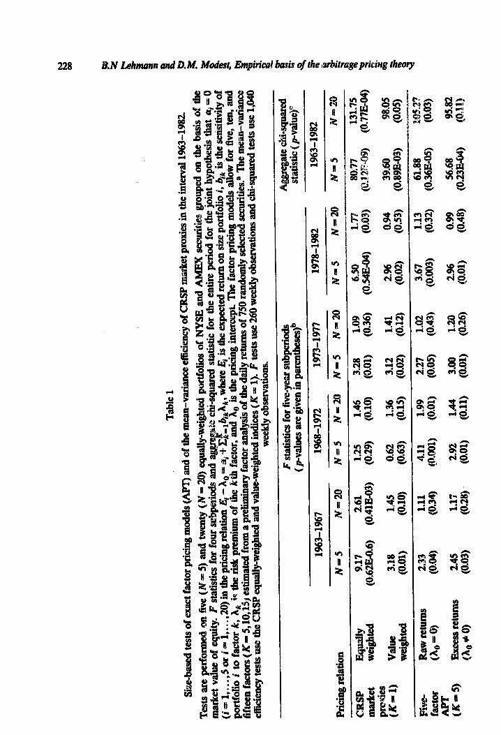
228 1% N khtnann ad D.iU. Mode@, Empirica! basis of the arbitrage pri&g theory
I I
, I
,
r r c
5 Y
I

B. N khmmn lad D. M. Mdest, Empirical basis of the arbitrage pric@g thewy 229

Tab
le 2
Siz
e-ba
sed
test
s of
exa
ct f
acto
r pr
icin
g m
odel
s (A
PT
) us
ing
diff
eren
t fac
tor
esti
mat
es a
nd o
f th
e m
ean-
vari
ance
eff
icie
ncy
of C
USP
mar
ket p
roxi
es in
th
e in
terv
al 1
963-
1982
.
Tes
ts a
re p
erfo
rmed
oti
tie
qu
ail
y-w
e&k&
d po
rtfo
tios
of
NO
SE a
nd A
ME
YC
secu
riti
es g
roup
&
_- o
n th
e ba
sis
of t
he m
arke
t val
ue o
f eq
uity
. F
stat
isti
cs
for
four
sub
peti
ods
and
aggr
egat
e cl&
squa
red
stat
isti
c fo
r th
e eh
e pe
riod
for
the
join
t hy
poth
esis
tha
t ui
= 0
(i
= 1,
. . .
,5)
in’ t
he p
rici
ng r
elat
ion
Ei -
X
0 =
ai +
Z&
lbjh
X,;
whe
re I
$ is
the
exp
ecte
d re
turn
OIP &e portfallio
i, 6ik is
the
seu
siti
vity
of
port
folio
i t
o fa
ctor
k,
X,
is t
he r
isk
prem
itim
of
thz
k*&
fact
or,
and
a0 i
s th
e pr
icin
g in
ter&
@. T
he f
acto
r pr
icin
g m
odel
s al
low
for
fiv
e an
d te
n fa
ctor
s (K
= $
10)
esti
mat
ed f
rom
a p
relim
inar
y an
alys
is o
f th
e w
eek
ly a
nd
mon
thly
ret
urns
of
750
rand
omly
sel
ecte
d se
curi
ties
.~ T
he m
ean-
vari
ance
eff
icie
ncy
test
s us
e th
e C
RSP
equ
ally
-wei
ghte
d an
d va
he~
wei
ghte
d in
dice
s (K
= 1
). F
tes
ts u
se 2
60 w
eekl
y ob
serv
atio
ns a
nd c
i&sq
ua~&
tes
ts v
m 1
,040
wee
kly
ob3?
:rva
tidn
s.
Pri
cing
rel
atio
n
.
1963
-l&
7
We&
y M
oz~t
bly
F s
tati
stic
s for
five
-yea
r sub
peri
ods
(p-v
alue
s ar
e gi
ven
in p
aren
th~5
5s)~
1968
-197
2 19
73-1
977
W&
ly
Mon
thly
W
eek
ly
Mon
thly
Agg
rega
te &
i-sq
uar
ed
stat
isti
c (p
-val
ue)”
1978
-198
2 -
196=
82
-I.
Wee
kly
M
a&&
y#
&..y
r.
r -
- ..
_.-
MO
KlU
ii~
’ C
RSP
J%
dY
9.17
9.
17
1.25
1.
25
3.28
3.
28
6.50
6.
50
80.7
7 80
.77
mar
La
W4figbd
(0.6
2E-O
.6)
(0.6
2E-0
6)
(0.2
9)
(0.2
9)
(0.0
1)
(0.0
1)
(O.S
4E-0
4)
(OS
4E-0
4)
(O.l
2E-0
9)
(O.l
2E-0
9)
prox
ies
(K-=
1)
va
lue
3.18
3.
18
0.62
0.
62
3.12
3.
12
2.96
2.
96
39.6
0 39
.60
Wt?igh!d
(0.01)
(O+
Ol)
(0
.63)
(0
.63)
(0
.02)
(O
&2)
(0
.02)
(0
.02)
(0
.89E
-03)
(0
.89E
-03)

Fiv
e R
aw r
etur
ns
3.32
3.
29
3.79
2.
00
4.32
3.
31
4.82
4.
04
81.2
5 63
.20
fact
or
(%I
= 0
) (0
.64E
-02)
(0
.68E
-02)
(0.
2SE
-02)
(0
.08)
(0
.86E
-O 3;
(W6E
-02)
(0
.31E
-03)
(O
.lS
E-0
3) (
0.24
E-0
8)
(0.2
3E-0
5)
(K-5
) E
xces
sret
urns
3.
10
3.47
3.
07
2.80
3.
61
2.83
4.
21
2.32
69
.95
57.1
0 (A
, #
0)
(0.9
9E82
) (0
.48E
-02)
(0
.01)
(0
.02)
(0
.36E
-02)
(0
.02)
(O
.llE
-02)
(0
.04)
(0
.19E
-06)
(0
.2O
E-0
4)
Ten
- R
aw r
etur
ns
4.58
28
0 3.
30
1.77
3.
45
2.47
3.
52
3.49
74
.25
52.6
0 fa
ctor
(A
, =
0)
(0.5
2E-0
3)
(0.0
2)
(0.6
7E-0
2)
(0.1
2)
(0.4
9E-0
2)
(0.0
3)
(0.4
4E-0
2)
(0.4
7E-0
2)
(0.3
4E-0
7)
(0.9
3E-0
4)
AP
T
(K=
lO)
Exc
egsr
etur
ns
.t 3
7 3.
36
3.72
2.
89
4.20
2.
26
3.38
2.
99
73.8
5 57
.50
(A,
+ 0
) (0
.4&
2)
(0.5
9E-0
2) (
0.29
E-0
2)
(0.0
1)
(O.l
lE-0
2)
(0.0
5)
(0.5
7E-0
2)
(0.0
1)
(0.4
2E-0
7)
(0.1
7E-0
4)
‘The
es
tim
ated
fac
tor
mod
el i
s us
ed t
o co
mpu
te p
ortf
olio
wei
ghts
whi
ch a
re c
ombi
ned
wit
h th
e w
eek
ly r
etur
ns o
f th
e 75
0 se
curi
ties
to p
rodu
ce
wee
kly
est
imat
es o
f th
e fa
cto=
bE
ach
F st
atis
tic is
for
the
test
of
the j
oint
hyp
othe
sis t
hat
ui =
0 in
the
app
ropr
iate
pric
ing
rela
tion
. For
the
AP
I’ te
sts,
the
~~
~ah
te is t
he p
roba
bili
ty
of o
btai
ning
a r
eali
zati
on g
reat
er th
an t
he t
est s
tati
stic
from
an
F di
stri
buti
on w
ith
N n
umer
ator
deg
rees
of
free
dom
and
235
- K
- N
den
omin
ator
de
gree
s of
free
dom
. For
the
CR
SP
mea
n-va
rian
ce e
ffic
ienc
y tes
ts, t
he p
-val
ue i
s th
e pr
obab
ilit
y of
obt
aini
ng a
rea
liza
tion
grea
ter t
han
the
test
sta
tist
ic
from
an
F di
stri
buti
on w
ith
N -
1 n
umer
ator
deg
rees
of
free
dom
and
235
- N
den
omin
ator
deg
rees
of
free
dom
. ‘E
ach
x2 s
tati
stic
for
the
ste
ti
me
peri
od is
N t
imes
the
sum
of
the
four
sub
peri
od F
sta
tist
ics.
The
pval
ue u
mbe
r ee&
x2
%id
ic
is t
he
prob
abil
ity
of o
bWun
g a
real
izat
ion
grea
ter t
han
the
test
sta
tist
ic fr
om a
x2
dist
ribu
tion
wit
h de
gree
s of
free
dom
equ
al t
o 20
whe
n N
= 5
and
80
whe
n N
= 2
0 fo
r th
e A
PT
test
s and
wit
h de
gree
s of
free
dom
equa
l to
16 w
hen
N =
5 a
nd 7
6 w
hen
N =
20
for
the
CR
SP
mea
n-va
rian
ce e
ffic
ienc
y tes
ts.

Tab
le 3
Siz
e-ba
sed
test
s of
exa
ct f
acto
r pr
icin
g m
odel
s (A
PT
) an
d of
the
mea
n-va
rian
ce e
ffic
ienc
y of
CR
SP
mar
ket
pro
ties
in
the
inte
rval
L96
3A98
2,
excl
udk
g Ja
nuar
y ret
ums.
Tes
ts a
re p
e&m
ed
0~ t
ie
(N =
5)
and
twen
ty (
N =
39)
qy_TMeighted
port
foli
os o
f W
SE
an
d A
ME
X s
ecm
itk
s gr
oupe
d on
the
bas
is o
f th
e m
ark
et v
alue
of
equi
ty.
F st
atis
tics
for
four
sub
peri
ods
and
te &
i-sq
uare
d statistic for
the
enti
re p
erio
d fo
r th
e jo
int
hypo
thes
is t
hat
ai =
0
(i=
l,..
.,
Sor
i==
l,...
, 20
) in
the
p&&
g re
lati
sn E
i ag
gry
- A
, = U
i + x
k_lb
ikX
k, w
here
Ei i
s the
exp
ecte
d re
turn
011
S&
po
rtfo
lio
i, b
ik is
the
sea
sitit
ity
of
poti
olio
i
to f
acto
r k
, A
, is
the
ris
k p
rem
ium
of
the
kth
fac
tor,
and
X,
is t
he p
rici
ng in
terc
ept.
me
fact
or p
rici
ng m
odel
s al
low
for
fiv
e, te
n, a
nd
fift
een
fact
ors (
K =
$10, 15
) est
imat
ed fr
om a
pre
lim
imuy
fac
tor a
naly
sis o
f th
e da
ily
ret~
tns o
f 75
0 ra
ndom
ly se
lect
ed se
curi
tka
The
mea
n-va
rian
ce
effi
cien
cy te
sts
use
the
CR
SP
equa
lly-
wei
ghte
d and
val
uew
eigh
ted
indi
ces (
K =
1).
F t
ests
use
260
wee
kly
obs
erva
tion
s and
&i-
squa
red
test
s us
e 1,
040
wee
kly
0bs
erva
tkM
UL
Pri
cing
rela
tion
F s
tati
stic
s fez
five
-yea
r sub
peri
odsb
A
ggre
gate
&i-
squa
red
(~V
a&E
!s ar
e gi
vez
k p
SeA
!ses
) st
atis
tic (
p-va
lue)
=
1963
01%
7 19
68-1
972
1973
-197
7 19
78-1
982
h%3-
1982
N=
=5
Iv=
20
N=
5 N
=2O
N
=S
N
=20
N=j
N=
20
N=
S
N--
20
-ZR
$P
prox
ies
W=
1)
W&
Y
6.15
1.
94
0.26
1.
40
0.87
0.
76
4.44
1.
36
46.8
3 10
3.77
W
iSig
htd
(O
.lO
EA
I3)
(0.0
1)
(0.9
1)
(0.1
3)
(0.4
8)
(0.7
5)
(0.0
02)
(0.1
5)
(0.7
2E-0
4)
(0.0
2)
Val
ue
1.98
I.
08
0.20
1.
51
1.56
1.
01
2.38
0.
79
30.5
7 83
.35
Wei
gh
ted
(0
.10)
(0
.37)
(0
.94)
(0
.09)
(0
.19)
(0
.45)
(0
.05)
(0
.72)
(0
.06)
(0
.26)
Fiv
e-
Raw
ret
urns
1.
37
0387
2.
01
1.54
1.
47
0.93
3.
56
I.13
42
.08
89.4
2 I;
?‘,*
= 0
) (0
.24)
(0
.6q
@08
) (0
.07)
(0
.20)
(0
.55)
(O
*OW
(0
.32)
(0
.003
) (0
.22)
W=
5)
E
xces
s ret
urns
1.
76
OH
1.
22
1.12
2.
12
1.12
3.
45
1.07
42
.76
84.8
9 &
#
0)
(0.1
2)
(O* W
(0
.30)
(0
.33)
(O
-06)
(0
.33)
(0
.005
) (0
.39)
(0
.002
) (0
.33)

T-0
R
aw re
turu
s 20
6 0.
95
1.68
1.
37
0.89
0.
78
2.22
0.
n 34
.24
77.5
5 fa
ctor
(A
0 = 0
) (O
-07)
(0
.53)
(0
.14)
(0
.14)
(0
.49)
(0
.73)
(0
.05)
(0
.74)
(0
.03)
(0
.56)
= (K
=
10)
Exc
essr
etur
us
1.81
0.
88
1.80
1.
26
1.12
0.
87
2.29
0.
78
35.1
4 75
.66
(ho
# 0
) (0
.11)
(0
.61)
(0
.11)
(0
.12)
(0
.35)
(0
.63)
(0
.05)
(0
.74)
(0
.02)
(0
.62)
Fif
teeu
- R
aw M
ums
206
0.85
1.
01
1.17
0.
87
0.70
2.
52
0.92
32
.26
72.7
9 fa
ctor
(h
o =
0)
(090
7)
(0.6
5)
(0.4
1)
(0.2
8)
(0.5
0)
(0.8
2)
(0.0
3)
(0.5
7)
(0*0
4)
(0.7
0)
(K=
lS)
Exc
ess r
etur
us
1.89
0.
81
1.23
1.
04
1.08
0.
74
2.21
0.
78
32.9
6 67
.47
(X0 #
0)
(0.1
0)
(0.7
1)
(0.2
9)
(0.4
1)
(0.3
7)
(0.7
8)
(0.W
(0
.73)
(0
*04)
(0
.84)
‘The
est
imat
ed fa
ctor
mod
el is
use
d to
com
pute
porG
otio
wei
ghts
whi
ch a
re c
ombi
ned w
ith
the
wee
kly
retu
ms o
f th
e 75
0 se
curi
ties
to p
rodu
ct
wee
kly
esti
mat
es of
the
fact
ors.
bE
ach
F st
atis
tic is
for t
he te
st of
the j
oiut
hyp
othe
sis th
at a
, = 0
in
the
appr
opri
ate p
rici
ng re
lati
ort.
For
the A
PT
test
s, th
e p-v
alue
is th
e pro
babi
ity
of o
btai
&g
a C
gr
catc
r tha
u th
e te
st st
atis
tic f
rom
au F
&&
ibuh
n w
ith
N n
umer
ator
degr
ees o
f fr
eedo
m au
d 26
0 - X
- iV
deuo
min
aiw
r de
gree
s of f
reed
om. F
or th
e CIU
P m
ean-
vari
auce
effi
cien
cy test
s, th
e p-v
alue
is th
e pro
babi
lity
of o
btai
niug
a re
ahza
tior
t gtea
ter t
hau
the
test
stat
isti
c fr
om a
u F
&tr
ibut
ion
wit
h N
- 1
uum
erat
or de
gree
s of f
reed
om au
d 26
0 - N
deu
omiu
ator
degr
ees o
f fre
edom
. %
a&
x2 s
tati
stic
for
the
aggr
egat
e tim
e per
iod i
s N
ti
mes
the
sum
of
the
four
subp
erio
d F s
tati
stic
s. Th
e p-
valu
e und
er e
ach
x2 s
tati
stic
is t
he
prob
abil
ity o
f ob
taiu
iug a
rea
liza
tiou
grea
ter t
hau
the
test
stat
isti
c fro
m a
x2
dist
ribu
tion
wit
h de
gree
s of
free
dom
equa
l to
20 w
hen
N =
5 a
nd 8
0 w
hen
N =
20
for t
he A
PT
test
s aud
wit
h deg
rees
of fr
eedo
m eq
ual t
o 16
whe
n N
= 5
and
76
whe
n N
= 2
0 fo
r the
CR
!W ux
au-v
aria
ucc e
tRci
eucy
test
s.

Tab
le 4
test
s of
exa
ct f
acto
r pr
icin
g m
odel
s (A
PT
) an
d of
the
mea
n-va
rian
ce e
ffic
ienc
y of
CR
SP
mar
ket
pro
xies
in
the
inte
rval
19
63-1
982.
Tes
ts a
re p
erfo
rmed
OR
five
(N
= 5
) an
d tw
enty
(N
= 2
0) e
qual
ly~
wei
ghte
d por
tf&
os
of N
YS
E a
nd A
ME
X s
ec~
niti
es gr
oupe
d on
the
bas
is o
f di
vide
~~
&y.
i&!.~
F s
tati
stic
s fo
r fo
ur s
ubpe
riod
s ad
aggr
egat
e &i-
squa
red
stat
isti
c fo
r th
e en
tire
per
iod
for
the j
oint
hyp
othe
sis
that
ai =
0 (
i =
1,.
. . ,5
or
i=
,...
,20)
ia
the
pzic
ing
rela
tion
Ei -
X
0 =
Ui +
Zf-
lb,X
, 9 w
here
Ei
is th
e ex
pect
ed n
etw
n
OII
div
iden
d-yi
eld
pott
foli
o i,
bik
is t
he
sen
siti
vity
Of
port
foli
o i
ta fa
ctor
k, A
, is
the r
isk p
rem
ium
of
the
kth
fac
tor,
and
X0
is t
he p
rici
ng in
terc
ept.
The
fac
tor
pric
ing
mod
els
allo
w f
or f
ive,
ten,
and
fi
ftee
n fa
ctor
s (#
= 5
, IO
, 15)
est
imat
ed fr
om a
pre
lim
inar
y fac
tor a
naly
sis o
f th
e da
ily
retu
rns o
f 75
0 ra
ndom
ly se
lect
ed se
curi
ties
! T
he m
ean-
vari
ance
ef
icie
ncy
test
s us
e th
e C
RS
P eq
~~
IIy~
w@
hted
and
valu
e-w
eigh
ted i
ndim
(K
= 1
). F
tes
ts us
e 26
0 w
eek
ly o
bser
vati
ons a
nd &
i-sq
uare
d te
sts
use
1,04
0 w
eek
ly o
bser
vati
ons.
-r
F
stat
isti
cs fo
r fi
ve-y
ear s
ubpe
riod
s A
ggre
gate
chi~
squa
red
(~~
a&s
are
give
n in
par
enth
eseQ
c st
atis
tic
( pqv
alue
)d
, 1%
3-19
67
1968
-197
2 19
73-1
977
1978
-198
2 19
63-1
982
Pri
cing
rela
tion
N
=5
N=
20
N=
5 N
=20
N
=5
N=
20
N=
5 N
=20
N
=s
Iv=
20
CR
SP
E
qual
ly
9.54
2.
40
0.96
0.
55
3.43
x.
21
7.58
2.
56
86.0
8 12
7.78
m
ark
et
Weig
hte
d
(0.3
3M)
(0.0
01)
(0.4
3)
(0.9
4)
(0.0
09)
(0.2
5)
(0.8
8E=
O5)
(0
.5lE
=O
3)
(O.l
SE
~lO
) (O
.l9E
-03)
pr
oxie
s &
x=
l>-
V&
R
2.18
1.
13
0.26
0.
44
2.64
1.
03
2.46
1.
02
30.1
5 68
.72
=&
*@i
(MU
) (0
.32)
(0
.90)
(0
.98)
(0
.04)
(0
#43
) (0
.05)
(O
-44)
(0
.02)
(0
.71)
Fiv
e-
Raw
re&
cns
1.47
0,
91
1.70
x.
11
1.56
0.
80
0.77
0.
69
27.4
8 70
.11
fW
(X0
e 0)
(s
.20)
(0
.57)
(0
.14)
(0
.35)
(0
.17)
(0
.71)
(0
.57)
(O
-84)
(0
.12)
(0
.78)
W=
5)
E
xces
s ret
urns
1.
44
0.92
0.
80
0.62
1.
76
0.73
1.
20
0.77
25
.99
61.0
1 (h
.0 f
0)
(0.2
1)
(0.5
6)
(0.5
5)
(0.8
9)
(0.1
2)
(0.7
9)
(0.3
1)
(0.7
5)
(0*1
7)
(0.9
4)

Ten
- R
aw r
etur
ns
2.67
1.
19
1.10
0.
96
0.85
0.
55
1.58
0.
70
31.0
1 67
.87
fact
or
(A,
= 0)
(0
.02)
(0
.26)
(0
.36)
(0
.52)
(0
.52)
(0
94)
(0.1
7)
(0.8
3)
(0%
) (0
.83)
(K= 1
0)
Exc
ess
retu
rns
2.44
1.
12
0.58
0.
54
0.97
0.
55
I.12
0.
67
25.5
4 57
.69
(&I
if 0
) (0
.04)
(0
.33)
(0
.72)
(0
.95j
(0
~4)
(0.9
4)
(0.3
5)
(0.8
5)
(0.1
8)
(099
7)
Fif
teen
- R
aw r
etur
ns
2.65
1.
15
0.64
0.
75
1.07
0.
54
1.56
0.
68
29.6
2 62
.32
fact
or
(k,
= 0)
(0
.02)
(0
.30)
(0
.67)
(0
.77)
(0
.38)
(0
.95)
(0
.17)
(O
-85)
(0
‘08)
(0
.93)
(K=15)
Eluxssretums 2
.51
1.12
0.
48
0.52
1.
15
0.51
1.
05
0.64
25
.96
55.5
9 (&
I +
Oj
(0.0
3)
(0.3
3j
(0=7
9)
(O*%
j (0
.33)
(0
0%)
(0.3
9)
(0.8
8)
(0.1
7)
(0.9
8)
“The
Grs
t por
tfol
io i
s an
equ
ally
-wei
ghte
d po
rtfo
lio o
f th
ose
stoc
ks t
hat p
aid
no d
ivid
ends
k
the
prec
edin
g pe
riod
. The
rem
aini
ng fo
ur o
r ni
nete
en
port
folio
s ar
e eq
ually
-wei
ghte
d po
tiol
ios
of t
he r
emai
ning
stoc
ks r
anke
d by
the
ir d
itid
end
yiei
d.
bThe
est
imat
ed f
acto
r m
odel
is
used
to
com
pute
por
tfol
io w
eigh
ts w
hich
are
com
bine
d w
ith t
he w
eekl
y re
turn
s of
the
750
sec
urit
ies
to p
rodu
ce
wee
kly
esti
mat
es o
f th
e fa
ctor
s.
‘Eac
h F
sta
tist
ic is
for
the
test
of
the j
oint
hyp
othe
sis
that
q =
0 in
the
app
ropr
iate
pric
ing
re&
&on
. For
the
AH
’ te
sts,
the
p_V
atue
is t
he p
roba
biht
y of
obt
aini
ng a
rea
lizat
ion
grea
ter t
han
the
test
sta
tist
ic f
rom
an
F d
istr
ibut
ion
with
N n
umer
ator
deg
rees
of
fr&
om
and
260
- K - N d
enom
inat
or
degr
ees
of f
reed
om* F
or t
he C
RSP
mea
n-va
rian
ce e
ffic
ienq
f tes
ts, t
he p
evab
te is
the
pro
babi
lity
of o
btai
ning
a r
ealiz
atio
n gr
eate
r tha
n th
e te
st s
tati
stic
fr
om a
n F
dis
trib
utio
n w
ith _
W Y 1
num
erat
or d
egre
es o
f fr
eedo
m a
nd 2
60 -
N d
enom
inat
or d
egre
es o
f fr
eedo
m.
dEac
h x2
sta
tist
ic f
or t
he a
ggre
gate
tim
e pe
riod
is N
tim
es t
he s
um o
f th
e fo
ur s
ubpe
riod
F s
tati
stic
s. T
he p
-val
ue u
nder
eac
h x2
sta
tist
ic i;
i; th
e pr
obab
ility
of
obta
inin
g a
r&Ji
zati
on gr
eate
r tha
n th
e te
st s
tati
stic
fro
m a
x2
dist
ribu
tion
with
deg
rees
of
free
dom
equ
al t
o 20
whe
n N
= 5
and
80
whe
n N
= 2
0 fo
r th
e A
PT
’ tes
ts a
nd w
ith d
egre
es o
f fr
eedo
m eq
ual t
o 16
whe
n N = 5
and
76
whe
n N
= 2
0 fo
r th
e C
RSP
mea
n-va
rian
ce e
ffic
ienc
y te
sts.

Tab
le 5
0wn
wu
ian
F’-b
ased
te
sts o
f ex
act
fact
or p
rici
ng m
odel
s (A
PT
) and
of
the
mea
n-va
rian
ce e
ffic
ienc
y of
Cm
P
mar
ket
pro
xies
in t
he in
terv
al 1
963-
1982
.
Tat
s ar
e pe
rfor
med
on
five
(N
= 5
) an
d tw
enty
(N
= 2
0) e
quaU
y=w
eigh
ted po
rtfo
lios
of
NY
SE
an
d A
ME
X
secu
riti
es g
rou
ped
on
the
basi
s of
ow
xwar
hce
. F
stat
isti
cs fo
r fo
ur w
bpek
ds
and
qgre
g at
e ch
i~sq
uare
d sta
tist
ic fo
r th
e en
tire
p&
od
for
the j
oint
hyp
othe
sis
that
ai =
0 (
i =
1,.
. . ,5
or
i--
l ,.
..,2
O)i
nthe
pric
ingr
elat
i~
Ei-
$j=
$d_Z
kp1
ik
k,
Q x
w
here
Ei
is th
e ex
geC
&d M
Urn
On O
W!k
V&
B
PO
dOfi
O
is
bik
& &
e S#
Zd~
V@
Of
pa
rtfo
lio
i
t0
fact
or k
, xk
is
the
risk
pre
rmut
u of
the
kth
fac
tor,
and
ho
is t
he p
rici
ng in
terc
ept.
The
fac
tor
pik
ing
mod
els
aNow
for
five
, ten
, and
fi
ftee
n fa
ctor
s (K
= S
,lO
, 15)
est
imat
t fr
om a
pre
lim
imuy
fac
tor a
na@
is o
f th
e da
ily
retu
ms
of 7
50 ra
ndom
ly s
elec
ted
secu
ritk
~~
The
mea
n-va
rian
ce
effi
cien
cy te
sts
use
the
CR
SP
equa
Uy=
wei
ghte
d and
valu
e-w
eigh
ted i
ndic
es (K
=
1). F
tes
ts us
e 26
0 w
eek
ly o
bser
vati
ons a
nd c
hi=
sqna
red t
ests
use
1,0
40
wee
kly
obs
erva
tion
s.
F s
tati
stic
s for
five
-yea
r sub
peti
ods
(Pva
pues
are
giv
en ti
yti
entk
~~
$~
Agg
rega
te ch
i-sq
uare
d st
atis
tic
(p-v
alue
)=
1%3-
185%
19
68-1
972
1973
-197
7 19
78-1
982
1%3-
1.98
2
Pric
ing
rela
tion
N
=5
N=
2!!
N-5
@
‘=a
N=
5 N
=2(
1,
--i-
=5
N,2
0 N
35
N=
20
CR
SP
m
ark
et
prox
ies
(K=
l)
Q&
Y
9.05
2.
75
1.14
0.
93
2.39
1.
10
6.86
1.
95
81.7
1 12
7.94
W
t!ig
h&!d
(0
.7F
M6)
(O
.l9E
-Q3)
(0
.34)
(0
.55)
(0
.05)
(0
.35)
(0
.3O
E-0
4)
(0.0
1)
(0.8
2E-1
0)
(0.1
8Eo3
)
Val
ue
3.27
1.
82
0.35
0.
78
1.56
0.
98
2.36
1.
03
30.1
7 87
.38
Wei
ghte
d (0
.01)
(0
.02)
(O
&Q
(0
.73)
(0
.19)
(0
.49)
(0
.05)
(0
.43)
(0
.02)
(0
.18)
Fiv
e fa
ctor
(K=
5)
xaw
re
turn
s 1.
70
1.55
1.
38
0.77
1.
55
0.75
1.
15
0.70
28
.88
75.5
0 (A
, =
0)
(0.1
3)
(0.0
7)
(0.2
3)
(0.7
5)
(0.1
8)
(0.7
7)
(0.3
4;
(0.8
2)
(090
9)
(0.6
2)
Exc
essr
etu
ms
1.70
1.
55
0.53
0.
47
1.72
0.
76
0.65
0.
62
22.%
67
.98
(ho
90)
(0.1
4)
(0.0
7)
(0.7
5)
(0.9
8)
(0.1
3)
(0.7
6)
(0.6
6)
(0.9
0)
(0.2
9)
(0.8
3)
.

clr-
sv
aw=
Raw
r,4%
urnn
2.
15
1.50
0.
74
0.60
0.
51
0.48
0.
36
0.49
18
.80
61.2
0 fa
ctar
(&
) - 0
) (0
%)
(0.0
8)
(0.6
0)
(0.9
1)
(0.7
7)
(0.9
7)
(0.8
8)
(097
) (0
.53)
(0
94)
(K=
10)
Exc
essr
etur
ns
1.90
1.
39
0.48
0.
48
0.89
0.
52
0.39
0.
49
18.3
0 57
.75
(WO
) @
.iO)
(0.1
3)
(0.7
9)
(0.9
7)
(0.4
9)
(O.%
) (0
.85)
(0
.97)
(0
.57)
(0
.97.
)
Fift
een-
R
aw re
turn
s 1.
96
1.35
0.
73
0.62
0.
63
0.50
0*
25
0.56
17
.84
60.4
2 fa
ctor
(A
, = 0
) (O
-09)
(0
.15)
(0
.60)
(0
.90)
(0
.68)
(0
.97)
(0
994)
(0
.93)
(0
.60)
(0
.95)
(K=
= 1
5)
Exc
essr
etur
ns
1.81
1.
28
0.67
0.
54
0.91
0.
50
0.32
0.
48
18.5
4 56
.18
(A, #
0)
(0.1
1)
(0.1
9)
(0.6
5)
(0.9
5)
(0.4
7)
(O.%
) (0
.90)
(0
.97)
(0
.55)
(0
.98)
VIu
z es
tim
ated
fact
or m
ode1
is u
sed
to c
ompu
te po
rtfo
lio w
eigh
ts w
hich
are
com
bine
d wit
h th
e w
&y
retu
rns o
f th
e 75
0 se
curi
ties
to p
rodu
ce
wee
kly
esti
mat
es of
the
fact
ors.
%
a&
F s
tati
stic
is
for
the
teat
of t
he jo
int h
ypot
hesi
s that
a, - =
0 i
n th
e ap
prop
riat
e pric
ing r
elat
ion.
For
the A
PT
test
s, th
e p-v
alue
is th
e pro
babi
lity
of o
Wai
nin
g a
real
izat
ion
gre
ater
than
the
test
stat
isti
c fro
m an
F d
isti
buti
on w
ith
N n
umer
ator
degr
ees o
f fr
eedo
m an
d 26
0 -
K -
M d
enom
inat
or
degr
ees o
f fr
eedo
m. F
or th
e CR
SP m
ean-
vari
ance
efkk
ncy
test
s, th
e p-v
atue
is th
e p_&
&G
Iity
of o
btai
ning
a re
aliz
atio
n gre
ater
thsn
the
tet
stat
isti
c fk
xu a
n F
dis
trib
utio
n wit
h N
- 1
num
erat
or de
gree
s of
free
dom
and.
260
- N
den
omin
ator
degr
ees o
f fr
eedo
m.
‘Eac
h x2
sta
tist
ic fo
r th
e ag
greg
ate t
ime p
erio
d is
N t
imes
the
sum
of
t?e
four
subp
erio
d F s
tati
stic
s. T
he
p-va
lue
unde
r eac
h x2
sta
tist
ic is
the
pr
obab
ility
of o
btai
ning
a re
aliz
atio
n gre
ater
than
the
test
stat
isti
c fro
m a
xt
dist
ribu
tion
wit
h de
gree
s of
free
dom
equa
l to
20 w
hen
N =
S a
nd 8
0 w
hen
N =
20
for
the A
PT
test
s and
wit
h de
gree
s of f
reed
om eq
ual t
o 16
whe
n N
= 5
and
76
whe
n N
= 2
0 fo
r the
CR
SP m
ean-
vari
ance
efki
ency
tes
ts.
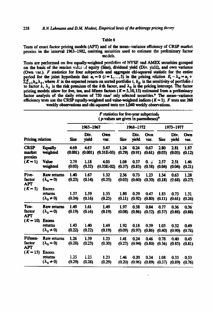
238 BAAI Lehmann and D. M. Modest, Empirical twis of the arbitrage pricing thmy
Table 6
Tests of exact factor pricing models (APT) and of the mean-vtiance efficiency of CRSP market proxies in the interval 1963-1982, omitting securitks used to estimate the preliminq factor
Tests are performed on five equally-weighted portfoxos & NOSE 2nd AMEX securities grouped on the basis of the market v&&~~f eq&y (Size), dividend yield (Div. yi&I), and own variance (Own var.). F statistics for four subperiods and aggregate c&qua& statistic for the entire period for the joint hy@ds that g-m0 (i-1,...,5) in the pti~@ &ti~n Ei-X,mai+ zf- 1 bik Xk 9 whm IZ is the errpected anUn 011 sorted PortfoliO s’, bik iS ahe S&!SJI Of pOdoK i to factor k, A, is the risk pre&m of the kth factor, ad X0 is the pricing intercept. The factor pricing models allow for five, tea. and Mteen factors (K = 5,10,15) estimated from a pAimimuy factor analysis of the daily returns of 750 rant amly selected securitka The mean-variance efficiency tests use the CRSP equally-weighted and value-wei@ed indices (K= 1). F tests use 260
weekIy *ations and chi-4uared &s& alce 1,040 weekly observations
F statistics for fin+year subperk& (JMN@esaregi!&qMuentbeses)b
Pricingrelation
1%3-1%7
Div. own size yield var.
1%~1972 1973-1977
Div. own Div. own Size yield var. !Sze yield var.
t”Rsp Epuauy market wreighted pties (K=l) value
weightted
4.69 4.67 5.47 1.24 0.24 0.67 2.80 2.81 1.87 (0.001) (0,001) (0.31E-03) (0.29) (0.91) (0.61) (0.03) (0.03) (0.12)
279 1.18 4.05 1.08 0.37 0. ,; 257 2.51 1.46 (0.03) (0.32) (0.33E-02) (0.37) (0.83) (0.58) (0.04) (0.04) (0.21)
Five- Rawretums 1.40 1.67 1.32 2.56 0.73 1.23 1.54 0.63 1.28 factor @PO) (0.23) (0.14) (0.25) (0.03) (0.60) (0.30) (0.18) (0.68) (0.27)
(K==5) Excess 1.37 1.59 1.35 1.80 0.29 0.47 1.83 0.73 1.31
(0.24) (0.16) (0.25) (0.11) (0.92) (0.80) (0.11) (0.61) (0.26)
Ten- Raw returns 1.49 1.61 1.49 1.97 0.38 0.84 0.77 0.36 0.36 factor (A, = 0) (0.19) (0.16) (0.19) (0.08) (0.86) (0.52) (0.57) (0.88) (0.88)
(K-10) Excess return!!! 1.43 1.40 1.49 1.92 0.18 0.39 1.03 0.32 0.49 (A, * 0) (0.22) (0.22) (0.19) (0.09) (0.97) (0.86) (0.40) (0.90) (0.78)
Fifteen- Raw returns 1.26 1.39 1.23 1.41 0.24 0.46 0.78 0.40 0.45 factor (&I = 0) (0.28) (0.23) ‘(0.30) (0.22) (0.94) (0.80) (0.56) (0.85) (0.81)
(K=15) Excess returns I.25 1.25 1.23 I.46 0.20 0.34 1.08 0.33 0.53 & + 0) (0.29) (0.28) (0.29) (0.20) (O.%) (0.89) (0.37) (0.89) (0.76)

Table 6 (contiaued)
F statistics for five-year subpeziods (pvaluesare~veninparentheses)b
Aggre&ate**qu statistic (JMhi&e)=
Pricingrdation
CRSP EBualtY market wei@ed proxies W= 1) Valut
*ted
5.06 4.73 5.47 55.19 49.86 53.92 (0.6lE-03) (0.001) (0.3lE-03) (0.33E-M) (OJ4E-04) (0.53E-UQ
1.$5 1.98 2.30 33.19 24.11 34.12 (0.12) (0.10) (0.W (O.oar) (0.09) (0.52E-u2)
Five- RaWrcturns 1.41 0.68 0.79 34.35 18.54 23.13 factar &-0) (0.22) (0.64) (0.57) (0*02) (0.55) (0.28) A?T <X=5) EXoesS
0.35 0.64 0.53 28.33 16.20 (0.58) (0.63 $H2) (0*09) (0.V (0.55)
Ten- RaWrrtunrs 1.03 1.34 0.63 z&34 18.47 16.58 factor (X0 e 0) WO) (OJ% (0.67) (0.15) to-=) (0.68)
(K=lO) Excess fetums 0.76 0.92 0.42 25.72 IBlO 13.95 (h#o) (O.f8) _ (0.43 (0.83) (0.18) (U.83) (0.53)
Fifkelb RaWmWllS 1.13 1.28 0.48 22.92 16.56 13.13 fix&M @,=O) (0.34) (0.27) (0.79) (0.29) (0.68) @=87)
(K==lS) Euzess 0.81 0.85 0.34 23.02 13.17 12.21
(0.W (0.52) (0.89) (0.29) $kq (Q.91)
bEa& Fsoalisticisfat~teStofthejohrth~thatuii~Oi;rtise~riatepricing relation. For the APT tests, the ~~alue is the probability of obtaining a reabatiori greater than the test statistic fkom an F distn’butiaa with N mameram ikgpiESOf~~and26U-K-N
denominator degrees of freedom, For the CRSP mean-varb~~ e&c&q tests, the p-value is the probability of obtaG.ng 4 &ization greater than the test e&istic from an F dis&ii~tron with N-laumeratordegreeso~~mand260-hldeMwninatordegreesofEreedom.
‘Eadr~~statisticfortheaggregaletimeperiadisNtimesthesumofthefowsubperiod F sMstics. The p-value under each x2 statistic is the probability of obtaining a realization grater than the test statistic from a x2 distr&ution wit& degrees of freedom equal to 20 when N = 5 and 80~~N=U)forthe~tests~d~~d~offreedom~~to16wi?ennr=Sand76 when Iv = 20 for tple CRSP mean-varbce eIkietlcy tests.

240 B. N Lehmann and 2 M. Modest, Empirical basis of the arbitrage pricing theory
yield, and o w~1 vaniafl~e. Each table reports the F statistics for both the rm-teturn and excess-return formulations of the AFT and for five-, ten-, ad
em-factor models. In tables present the large sample F of the CRSP equally-weighted and
value-Wtighred indices 0 relevant F statistic for
the four subperiod F statistics. 26 The mumber report& under each test
basisoffkmsize.The
spWi.ng the ranked securities into either five or twenty groups consisting of equal numbers, and then co~tructing equally-weighted port- stocks in each group. 27 Tables 2 and 3 provide the same
information as table 3, but serve as decks that the results in table 1 do not hinge on peculiar&ies jll,oivving thin trading or January. The! sole &fkrence between tables 1 and ri! that table 2 presents resuh,s wheL the factor mod& are estimated using week@ and monthly data rather than daily data. In a__ similar spirit, the tests in table 3 are based on returns that exclude those occurring in January to ensure that we are not confusing the turn-of-the-year and size effects. Tabk 4 is similar to the Grst table except that portfolios are formed GA the basis of dividend yield in the year preceding the test period. The e procedure is somewhat different as well, since we form an equally-weighted portfolio of the kms that paid zero dividends and then form the remaining four or nineteen portfolios by ranking the remaining dividend-
=The F statistics for the CRSP indices, derived in Shanken (1985b), diifer slightly from those givea in (6) for the APT tests. First, &* is the vector of residuals from the cross-sectional
et model ktercepts on one minus th_L estimated betas. The other is replaced with N - 1. Note that these statistics are formed from
the sorted portfolios and are subject to the potentid power diEulties discussed in the text. However, this does not sze,.n to be a problem in thi: application. . _
26The distrihiun or’ hi times an F statistic with Ad numeqtor degrees of freedom and N denominator degrees of om is tiudy ~&stingui&&~e from Q &&i&GGfi Rib
M degrees of freedom for ranging between 5 and 20 and deoq+ajis of freedom of at least 215.
27 also performed tests based (?LI ten such portfolios but the results were similar to those
obtained with either the five or twenty portfolios and so we omit them to conserve sbace.

paying stocks in the
the fmgind si&nificance levels subperiod results reveals consid spending subperiod F statistics that in&de &wary retums or correct for thin trading are large enough to rejed’t the APT at cmventional signifi@ance
or of the version of the
are large enough to r@xt in the subperiods as w&L29
‘*We also carried out tests by raking on dividend yield without trament of the zero dividend group. nitsalts were very
29The test!3 of excess-m versionof the alsodonotseemtohgeonwbe ft!tunrs~OO~tKUCted~thetzturnsO~&~
ortihogonal portfolio. w* excess re~~~~45 orthogonal portfolio, the correspond F statis factor x-e&s reported in table 1 for the four s and 3.3P(O.Oi) - alI not very Merent from F tests do, however, ignore the estimation error in the sample man return portfolios, imparting a MS of Untnomm direction and nqpimdc

2452 B.lV Lehmann and D.iU. Modest, Empirical basis of the czbitragqwicing theory
hese results are not just reflections of unusually large intercepts for the est firm (i.e., fifth quintile) portfolio. To be sure, this portfolio has large
as in all four periods. owever, the size e!Tect is not teo e fourth quintile appears to plot above t
the largest-firm portfolio consistently plots below the 1 rane. This aaagw- r-r p firm effect receives st g conforma-
eighted index on the basis portfolios, t iwtercepts on the order of - 2.5% to -4.5% per year
year period. Although some of this effect may be to nonstationanty associated v ’ th the changing weights of the
effect remains (albeit with lesser magnitude) when firm portfolio.
-variance efficiency of the equally-weighted and ed on five firm&,e portfolios provide similarly
umentation of the magnitude qf the size efkct. The aggregate x2 statistic rejects the mean-variance efficiency of the equally-weighted index at marginal significance levels below 10a9, and the same statistic constructed excluding January returns rejects at marginal signiknce levels below 10e4. The antiogous egate marginal signifkance levels for the tests of the mean-variance e ency of the value-weighted index are below 10m3 for the whole sample and at the 6% level when January returns are excluded. Again,
le uniformity in the subperiod results, since the mean-vari- ciency of both indices is rejected in all but the second period when returns are included and in the first and fourth periods when they are
e size-related results b on twenty portfolios reported under M = 20 in 1 tell a somewhat di nt story. The mean-variance efficiency of the
usual market proxies is rejected in aggregate at marginal significance levels for the equally-weighted index and at the 5% level for the
dex &I the whole sample, while only the equally-weighted level) when January returns are excluded. In
-return version of the five-factor model is
is no accident, since in

.
case were we
tabk 5, whkh exclude the 39 s ecurities that were used to const
at an aggregate marginal significance level near 2% and the five-factor e~cezz~- retui-fi W&III was marginally rejected at just over the 9% Ilevel, probably &kct the size of these subsamples - there are fewer very small firms with which to reject the theory.
The tests for the two report&! in table 4, reject euT mean-varian from the earlier work of Litzenberger and Elton, Goober, and
equally-weighted index at a mar
statistics reject the null hypothesis for both indices at conventional sign.%cance e mean-variance e
the equally-weighted index is also and in the subs
examination of

244 B.N &hmann ad D.M. A&&w, Empirical basis of the arbitrage pi&~ #wury
related portfolios. The only evidence against the theory in the individual subperiods occurs in the first sttbperiod: both versions of the ten- and fifteen-factor models are rejected at marginal significance levels between 2% %md 4% with five dividend-sorted portfolios. There is no evidence against the APT in the remaining five ,portfolio. results and no evidence at all in the twenty-i>ortfolio test statistics or those in table 6, which exclude the 750 securities used to create the basis portfolios.3o
The results for portfolios based on own variance mirror those obtained in the dividend-yield case. The mean-variance efficiency of the CRSP indices is rejected at almost identical marginal significance levels in most cases and more sharply for some of the r emaining statistics, particularly those relating to the value-weighted index. The AIT basis portfolios do not yield intercepts that are significant over the whole sample with the exception of the five-factor r;;c1w- return model which receives a marginal rejection at the 9% level. In addition, manv of the F statistics are marginally sig,nXcant (between the 6% and 10% level) in the first five-year period, although the remaining test statistics are typically grossly ins&&ant (many at the 90% level and larger). Again, the information in the test statistics is a reliable guide to the behavior of the individual portfolio intercepts, except perhaps for the highest own-variance portfolio, which has moderately large intercepts across three of the four subperiods = although they are not very precisely estimated and usually are statistically insignificant. The basic message is similar: the rejections of the mean-variance efficiency of both CIUB indices suggest the ability to reject some asset pricing models, and the failure to reject the APT pricing restriction suggests that the theory provides an adequate account of the risk and return of the own-variance portfolios.
Finally, in table 7 we present summary x2 statistics for the joint significance of the mean returns of the basis portfolios constructed from the five-, ten-, and fifteen-factor models. These x2 statistics are of interest, since the AIT implies that at least one of the factor risk premiums should be significantly different from zero under the assumption that investors are risk-averse. As is readily apparent, our large cross-sections yielded basis portfolios with highly signifi- cant mean returns in aggregate and in most of the individual subperiods as well. This is in sharp contrast to the frequency insignificant mean returns of basis portfolios constructed from smaller cross-sections.
3oExamination of the individual portfolio intercepts provides some evidence of positive (but usually insignificant) intercepts for the zero-dividend and high-dividend portfolios. In the tests based on twenty dividend-yiela portfolios, the intercepts for the remainiug portfolios often have mixed signs and are typically economically and statistically insiguificzu& Howevcr9 in the tests based ou five sorted portfolios: the lowest dividend-yield portfolio (excluding the zero-dividend portfolio) has on average the smallest intercept and the remaining intercepts increase in a monotonic fashion - producing a dividend~yield elTect that is qualitatively similar to the one found using the traditional market proxies, but not nearly so pronounced.

Tab
le 7
Tat
s of
the
join
t ti
gnik
ance
of
the
fact
or G
sk p
rem
bms
Ak
(k =
1,.
. . ,
K)
b th
e in
terv
al 1
663-
1982
.
chi-
squa
red
stat
isti
cs f
or f
our
subp
erio
ds a
nd f
or t
he e
ntir
e pe
riod
for
the
join
t hy
poth
esis
tha
t A
, =
0 (
k =
1,.
. . ,
K)
in t
he,:
pric
ing
rela
tion
E
i - A
@ = U
i + C
RK
llb,
khk,
whe
re E
i is
the
wtd
R
- O
n
secu
rify
i,
bik
b t
k
SeD
sitt
itiQ
~
of s
ecuf
ity
i to
faC
tOr k
, A
, is
the
&k
P
&W
O
f the
k
th f
acto
r, a
nd A
, is
the
prk
ibg
inte
rcep
t. T
he fa
bcto
r p&k
g m
& -
Is Z
&W
for
five
, te
3, a
nd f
ifte
en f
acto
rs (K
= S
,lO, 1
5) e
stim
ated
from
a p
reG
min
ary
fact
or a
nal@
of
the
dai
ly r
etur
ns o
f 75
0 ra
ndom
ly s
elec
ted
secu
riti
es!
The
snb
p&od
s co
&&
26
0 w
eek
ly o
bser
vati
ons
a&th
e w
hole
wk
. co
ntai
ns 1
,040
wee
kly
obs
erva
tion
s.
Chi
~4u
ared
sta
tist
ics f
or fi
ve-y
ear s
ubpe
riod
s (~
Val
ues
ate
gkn
in p
aren
&S
es)b
A
ggre
gate
chb4
uare
d st
atis
tic
(~va
lue)
=
Mci
ng r
euio
n .
1963
-196
7 19
68-1
972
1973
-197
7 19
78-1
982
1363
-198
2
Fiv
s?-
fact
or
Raw
retu
ms
(&I =
a)
20.5
3 (0
.99E
=O
3)
28.6
2 (0
.28E
-04)
_-
15.8
8 (0
.82E
AI2
) 12
.96
(0.0
24)
77.6
9 (O
.%E
-O8$
Exc
ess r
etur
ns
(X0 +
09
20.2
3 (O
.llE
-02)
Raw
retu
rns
(X0 -
01
Els
essr
etur
ns
(X0 f;
lo9
25.9
8 (0
.38E
-02)
27.2
8 (0
.233
-02)
3.27
(0
.66)
36.8
3 23
.25
(0.6
1E-0
4)
(0.9
9E-0
2)
12.8
5 (0
.23)
10
*36
(0.4
1)
7.56
(0
.18)
35.2
3 (O
.llE
-03)
23.3
5 (0
.95E
-02)
42.2
0 (0
.26E
-02)
121.
29
(0.4
iE-W
j
73.8
3 (0
.9C
E-0
3 j
- F
ifW
Xl-
R
aw-
35.4
8 49
.21
27.4
3 37
.48
149.
60
(X0
- 09
(0
.2lE
=O
2)
(0.1
6E-0
4)
{0#
025)
(O
.llE
-02)
(0
.13E
-08)
(Km
15)
E
WS
sfet
ums
35.5
2 21
.25
12.7
4 24
.58
94.1
0 (A
, #
09
(0.2
1E-0
2)
(0.1
3)
(0.6
2)
(0.0
56)
(0.3
2E-0
2)
“~~
%*s
~~
~i8
for~
~to
fthe
join
th~
~th
atX
,-O
(k~
l,...
, K
) in
the
app
ropr
iate
prW
g re
lati
on. T
he p
vatU
e is
the
pr
&bW
y of
obt
Jlin
ing a
rea
lizat
ion
gre
ater
than
the
test
st
atis
tic
from
a x
2 di
stri
buti
on w
ith
K d
egre
es o
f W
orn.
b&
ch
x2 s
tatk
tk
ftr
the
qgre
ga&
ti
me
peri
od i
s *&
e sum
of
the
four
sub
peri
od x
2 st
atis
tks.
The
p-v
alue
is
the
prob
abil
ity
of &
&i&
g a
. .
rcda
tm
gcea
ter
than
th
e te
st s
tMis
tic
from
a x
2 di
stri
butb
n w
ith
4K d
egte
es o
f M
orn.

246 B. N Lehmann~ and D. M. Modes, ~mpirdca~ basis of the arbitrage pricing theory

Tab
le 8
(co
ntin
ued)
-
F s
tati
stic
s for
five
-yea
r sub
peri
ods
(p-v
alue
s ar
e giv
en in
pai
cnth
eseQ
b A
ggre
gate
chi-
squa
red
stat
isti
c (J
Whl
e)’
Pri
cing
rela
tion
1978
-198
2
Div
. yie
ld
own
var.
S
ize
1963
-198
2
Div
. yie
ld
own
var.
Fiv
e-
Raw
ret
urns
7.
41
5.93
7.
36
127.
37
109.
40
102.
48
fact
or
(A,
= 0
) (O
.l7E
-05)
(0
.34E
-04)
(O
.l9E
-OS
) (O
.l2E
-16)
(0
.25E
-13)
(0
.45&
12)
(K=
5)
E
xces
s ret
urns
59
.78
142.
04
268.
89
685.
98
945.
24
2195
.00
(&I
+ 0
) (O
-00)
(O
=W
(O
=O
Q
WO
O)
(O=
OO
) (0
.00)
Ten
- fa
ctor
A
PT
(K
=
10)
Raw
ret
urns
0.
95
3.20
1.
68
28.0
2 59
.07
41.5
0 (&
I =
0)
(0.4
5)
(O.S
lE-0
2)
(0.1
4)
(0.1
1)
(0.9
9E-0
5)
(0.3
2E-1
2)
Exc
ess r
etur
ns
14.1
7 10
.10
13.3
3 27
6.43
25
6.54
23
3.36
(A
, f:
0)
(0.3
5E-1
1)
(0.8
3E-0
8)
(O.l
7E-0
6)
(0.W
(O
=O
Q
(0.2
3E-3
7)
Fif
teen
- R
aw r
etur
ns
1.45
2.
68
0.52
27
.37
38.7
2 27
.93
fact
or
(&I
= 0
) (0
.21)
(0
.22E
-01)
(0
.76)
(0
.13)
(0
.72E
02)
(Urn
) A
PT
(K
=
15)
Exc
ess ;
:tum
s 2.
57
2165
2.
18
192.
22
199.
12
AX
12
(&I
f 0)
(0
.027
) (0
.023
) (0
.058
) (0
.39E
-29)
(0
.17E
30)
(0.9
2Eo2
7)
‘The
es
tim
ated
fac
tor
mod
el i
s us
ed t
o co
mpu
te p
ortf
olio
wei
ghts
whi
ch a
re c
ombi
ned
wit
h th
e w
eek
ly r
etur
ns o
f th
e 75
0 se
curi
ties
to p
rodu
ce
wee
kly
est
ima+
~s o
f th
e fa
ctor
s.
bEac
b F
~tatktk is fo
r th
e te
st o
f th
e jo
int
hypo
thes
is t
hat
~~
_lbi
k =
1 i
n th
e ap
prop
riat
e pr
icin
g re
lati
on. T
he p
-val
ue i
s th
e pr
obab
ilit
y of
ob
tain
@
%I re
aliz
atio
n @
eate
r tha
n th
e te
st st
atis
tic f
rom
an
F di
stri
buti
on w
ith
5 nu
mer
ator
deg
rees
of f
reed
om a
nd 2
60 -
K -
5 d
enom
inat
or d
egre
es
of f
reed
om
‘Eac
h x2
sta
tist
ic f
or t
he a
ggre
gate
tim
e pe
riod
is N
tim
es t
he s
um o
f th
e fo
ur s
ubpe
riod
F s
tati
stic
s. Th
e p-
valu
e un
der
each
xz
stat
isti
c is
the
pm
bbili
ty
of
obta
inin
g a
real
izat
ion
grea
ter t
han
the
test
sta
tist
ic fr
om a
x2
dist
ribu
tion
wit
h de
gree
s of
free
dom
equ
al t
o 20
whe
n N
= 5
and
80
whe
n N
-
20 f
or th
e A
P’p
test
s and
wit
h de
gree
s of
free
dom
equa
l to
16 w
hen
N =
5 a
nd 7
6 w
hen
N =
20
for
the
CR
SP
mea
n-va
rian
ce e
ffic
ienc
y tes
ts.

Tab
le 9
Mea
ns, s
tand
ard
devi
atio
ns, a
nd t
sta
tist
ics f
or m
onth
ly r
etur
ns o
n T
reas
ury b
ills
and
on
orth
ogon
al p
ortf
olio
s in
the
inte
rval
1%
3-19
82.a
‘he
orth
ogon
aJ p
ortf
olio
s ar
e co
nstr
ucte
d to
hav
e m
inim
um v
aria
nce
and
retu
rns
unco
rrel
ated
wit
h th
e re
aliz
atio
ns o
f th
e co
mm
on f
acto
rs in
the
et
urn-
gene
rati
ng pr
W
Ri,
- E
i =Z
fml&
ikB
kr +
eit
, whm
R
i, is
the
ret
urn
of s
ecur
ify
i at
tim
e t,
Ei
is t
he e
xpec
ted
retu
rn O
II ~
W$t
y i,
6ik
is th
e en
&M
y of
sec
urit
y i
to f
acto
r k
, &
, is
the
rea
liza
tion
of
the
kth
fac
tor,
and
ei,
is t
he id
iosy
ncra
tic d
istu
rban
ce o
f se
curi
ty i
. Th
e fa
ctor
pri
cing
no
dels
all
ow f
or fi
ve, t
en, a
nd f
ifte
en fa
ctor
s (K
= 5
,10,
15)
esti
mat
qi f
rom
a p
reli
min
q fa
ctor
ana
lysi
s of
the
dGly
ret
urns
of
750
rand
&nI
y se
kct
ed
secu
riti
es.b
sum
mar
y S
tatis
tic
Sum
maq
sta
tist
ics f
or fi
ve-y
ear s
ubpe
riod
s io
r th
e ag
greg
ate
(p-v
alue
s ar
e gi
ven
in p
aren
thes
es)=
ti
me
peri
od
1963
-196
7 19
68-1
972
1973
-197
7 19
78-1
982
1963
-198
2
Y2
Std.
st
d t
Mea
Il
dev.
s;
t.
Mea
n de
v:
std.
t
std.
t
sib.
st
at.
Mea
n dc
v.
stat
. M
esa
dev.
st
at.
Mea
n ( p
-val
ue)d
Tre
asur
y bil
l ret
urns
0.
0033
0.
0005
6 45
.95
0.00
46 0
.001
1 33
.65
0.00
53 0
.001
1 36
.25
OAK
I 0.
0023
29.
36
0.00
55 5
420.
17
(O*O
@
(OJJ
@
(0.W
(O
=W
(O
=O
Q
Fiv
e-
Raw
ret
urns
-0
.000
55
0.01
8 0.
22
0.00
84 0
.022
3.
00
0.00
81 0
.022
2.
91
0.00
64 0
.022
2.
211
QO
O56
22
.41
fact
or
(0.8
2)
(0.0
027)
(0
.003
6j
(0.0
27)
(0.0
0017
)
(K=
5)
&cP
a -0
.003
9 -
1.59
0.
0039
-
1.36
0.
0028
-
1.01
-0
.002
4 -
0.82
O
.OoQ
l 6.
08
retu
rns
(0.1
1)
(0.1
7)
(0.3
1)
(0.4
2)
(0.1
9)
over
T
-bil
ls
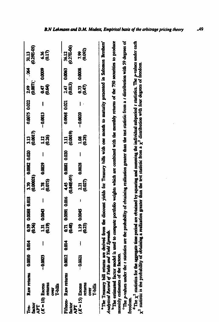
Ter
r-
Raw
ret
lu!N
0.
0011
0 0.
014
0.59
O
.W88
0.0
18
3.70
O
N82
0.
020
3.13
M
w?s
0.
022
269
J !.+
I64
31.1
3 fa
ctor
(0
.W
(0.o
oo21
) (O
.aw
) (o
.oon
: (0
.29E
-05)
(K=
lO)
Exc
ess
-0.0
023
- 13
1 0.
0043
-
1.78
0.
0029
-
1.12
-0
.001
3 -
0.47
o.
an!J
6.
36
retu
rns
(0.1
9)
(0.0
75)
(0.2
6)
(O*M
I (0
.17)
EZ
LS
Fif
teen
- R
aw a
twns
0.
0012
0.
014
0.7l
0.
0091
0.0
16
4.45
0.
0081
0.0
20
3.11
0.
0068
0.0
21
247
0.00
63
36.1
2 fa
ctor
(0
.48)
(0
.84E
-05)
(i
Mol
9)
(0.0
13)
(0.2
7E-0
6)
(K=
15
) E
xces
s -0
.QO
2i
- 1.
19
0.04
5 -
2.21
0.
0028
-
1.08
-0
.oo2
0 -
0.73
0.
0008
7.
99
retu
rns
(OW
(0
.027
) (0
.28)
.
(0.4
7)
(O.o
!n)
tYF
ii!s
aThe
Tm
ury
bill
ret
urns
are
der
ived
fro
m t
he d
isco
unt
yiel
ds f
or T
reas
ury
bill
s w
ith
one
mon
th t
o m
atur
ity
pres
ente
d in
Sal
omon
Bro
ther
s’
Ana
@id
R
eud
qf Y
iiel&
ad
YM
Spm
ds.
bath
e es
tim
ated
fw
tor
mod
el i
s us
ed t
o co
mpu
te p
ortf
olio
wei
ghts
whi
ch a
re c
ombi
ned
wit
h th
e m
onth
ly r
etur
ns o
f th
e 75
0 se
curi
ties
to p
rodu
ce
mon
thly
est
imat
es o
f th
e f&
ctor
s ‘T
he p
-val
ues
unde
r th
e t
stat
isti
cs a
re th
e pr
obab
ilit
y of
obt
aini
ng r
eali
zati
on gr
eate
r tha
n th
e te
st s
tati
stic
from
a t
dis
trib
utio
n w
ith
59 d
egre
es o
f fr
eedo
m.
dThe
x2
stat
isti
cs fo
r th
e ag
greg
ate t
ime
pezi
od a
re o
btai
ned
by s
quar
ing
and
sum
min
g th
e in
divi
dual
sub
peri
od t
stat
isti
cs. ‘
I%e p
valw
s un
der
each
x2
sta
tist
ic is
the
pro
babi
ity
of o
bt&
iog
a re
aliz
atio
n gre
ater
than
the
tes
t sta
tist
ic fr
om a
x2
dist
ribu
tion
wit
h fo
ur d
egre
es o
f fr
eedo
m.

250 B. N Lehmann ad D. .M Modest, Empirical basis of the arbittage pricing theory
5.3. Tests for spanning
Table 8 provides evidence on whether the K basis portfolios span the mean-variance effkient frontier of the individual assets. In particular, it reports the relevant test statistics for the hypothesis that the portfolios formed on the basis of firm size, dividend yield, and own variance have loazlings that sum to unity - an implication of mean-variance spanning. Attention is re- stricted to the results bas4 five such portfolios in order to conserve space, which involves little sacrifke, since the results for ten and twenty portfolios were much less favorable to this formulation. The results in table 8 suggest overwhelming rejection of the joint hypothesis that the raw-return formulation of the APT is correct and that the basis portfolios span the mean-variance efficient frontier and are measured without error. The aggregate test statistics based on excess return regressions reject the null hypothesis at marginal significance levels below 1O-27, and the least significant subperiod F statistic has a marginal significance level of 2.3%. The hypothesis fares only slightly better in the raw-return regressions - all but three of the eighteen aggregate test statistics have marginal significance levels below 0.002, as do many of the subperiod statistics. Moreover, these results are most favorable to this version of the APT - we would have made no such caveats had we chosen to report the twenty portfolio results.
5.4. I%e k&adot of the orthogonal pott&olios
Table 9 reports summary statistics on the sample behavior of the monthly returns on the orthogonal portfolios constructed from fivemi ten-, and fifteen- factor models anA d one-month Treasury bills. For each orthogonal portfolio a&&o for one-month Treasury bills, we report the mean return, the sampie standard deviation of its return, and the t statistic for the hypothesis that the mean return is significantly diEerent from zero. We also present the mean return md associated t statistic for the difference in returns between each orthogonal portfolio and o nemonth Treasury bilk. ‘Z”nese statistics are pre- sented for each of the four five-year periods. In addition, we present ap- proximate x2 statistics31 for the hypothesis that the mean returns are. jointly significantly different from zero across the four periods. In all cases we also report the marginal significance level of the test statistics.
The results in table 9 suggest considerable uniformity in the behavior of the orthogonal portfolios from the five-, ten-, az% fifteen-factor models The t
siatls~ics for a-x Y”it%rn retarm ruAaa~ cm the orthogonal portfolioo of all three factor
311t proved to be convenient with our software to produce these approximate x2 statistics instead of the usual F statistics. Fortunately, with these sanqk sizes the difference in marginal significance is very small.

-_
B.N Lehmann and D.M. Modest, Enapiricd baris of the arbitrage pricing theory 251
models are highly significant in the final three subperiods, although t&y ate
insignificant in the first period. The x2 statistics for the joint significance of the mean returns for each orthogonal portfolio across the four sample periods have marginal significance levels below lOa for each factor model. In con_ tradistinction, the corresponding t statistics for the differences in mean returns between these portfolios and the one-month Treasury bill are ins&n&ant in each subperiod with two exceptions: in the second subperiod, the mean return difference fcr the orthogonal portfolio from the ten-factor model is marginally sign&ant at the 7.5% level, whereas that from the fifteen-factor model is significant at the 2.7% level. In addition, these mean-return differences have mixed signs, negative in the Crst and fourth periods and positive in +&e middle two periods. Moreover, the aggregate x2 statistics for the joint signifkance of the mean-return differences have marginal significance levels of 0.19 for the five-factor model, 0.17 for the ten-factor znod4, and 0.892 for the fifteen-factor s
model. Only the fifteen-factor results reflect a marginal rejection of tlze hypothesis that this mean-return difference is zero, a rejection attributable solely to the results from the second subperiod.
The sun~~~ry statistics rcport& in table 9 indicate orthogonal portfolio returns with means that are signifkantly different from zero and insignificantly different from the mean return on one-month Treasury bills. This is additional evidence against the spanning model that is far more consistent with either of the excess-retm models rather than the mixed results obtain& by the previous authors, since most previous studies have been unable to fine statip);flQtl=r &rr&fi;r. UUWUUJ OaV.,ant pricing intercepts. -Moreover, these results stand in sharp contrast to those obtain& in studies ~4 the CAPM, where the estimated zero-beta rates are typically significantly greater than Treasury bill rates.
Finally, the sample standard deviations of these orthogonal portfolios are far from zero: typi&lly ten to thirty times those on one-month Treasury bills. This could arise for several reasons, as discus& in section 3.2.2. For example, the limiting minimum~variance portfolio could be riskless but our procedures are incapable of eliminating idiosyncratic risk ln Unite cross-sections. This interpretation is consistent with the observation that the mean returns on the orthogonal portfolios are typically insignificantly diflerent from those of one-month Treasury bills. Alternatively, the limiting minkmum-variance port- folio could be risky and, hence, it is shear happenstance that the mean returns on these portfolios are insignificantly different from one-month Treastu-y Ml rates. It is certainly worth noting that these mean returns are insignificantly different from many positive n~~mbers!
6. Conclusion
This paper is devoted to the accumulation of facts a_n,A, the sifting of evidence regarding +he validity of the APT in its various formulations. By far
252 RN Lehmann and D. M. Modest, Empirical basin of the arbitrage pricing theory
the most interesting results concern the validity of the API’ itself. The APT fares well when confronted with the strong relationship between average returns and either dividend yield or own variance. The APT provides an adequate account of the relation between risk and return of the dividend-yield and ow~ariance portfolios where risk adjustment with the usual CAPM market proxies fails. It is noteworthy that the APT provides a risk-based explanation of these phenornexa in contrast to the usual tax-related explana- tion of the dividend effect and the transitions-cost account of the relationship b&we3 own variance and average retums.32 In contradistinction, the tests .
hsed on firm size provide sharp evidence against the APT, although the form of size effect appears Merent from that documented in CAPM studies.
One interpretation of this failure to account for the size effect centers on sample size, asynchronous trading, or any of the 0th~ potential problems discussed earlier. We are persuaded, though, the large cross-sections that XT employ largely mitigate the effect of measurement error. Similarly, the thin. trading corrections yield no suggestion 4&at the size-related results are attr%W able to this problem. Moreover, the sharpness of the rejections reported in tables 1-3 suggests that they cannot be attributed to peculiar small-sample properties of the test statistics such as those that might result, for example, from nonnormality. These considerations suggest the failure of the APT to account for the size effect is credible.
The obvious interpretation is that we have rejected the exact factor pricing versions of the APT or9 to be more precise, our implementation of the theory. ‘I’he abilitv of a m~~~~re of wt=*ra+~~~:- yIpuf3~~~a~~~ risk to expiain risk-adjusted returns vi&a&s the theory. The concentration of the size effect in the very smallest and largest tims, however, suggests at least one potential alternat& explanation of these results. Suppose there is a small-firm factor, in that the business-cycle risk of small firms, especially *those primarily traded over the counter or closely held, is much greater than that of larger firms. In addition, suppose that the exposure to this source of risk is small for most listed quities but that the risk premium for this factor is positive and large.33 In these circumstances, our procedures for estimating the common factors would fail to measure this factor well, since few &IKE in our cross-s&on would be materially affected by it. Hence, this account of the size effect involves measurement error in the factors, measurement error that follows from the assets selected for the analysis rather than arising from our statistical proa-
321t is possible *hat the absence of a measured dividend effect in our APT results is consistent with the tax story. This could occur, for example, if one of the risk factors reflected random marginal tax rates impinging on asset pricing and the corresponding factor loadings arc the dividend yields of the individual securities.
33“f’his scenario is5 in principle, consonant with our rqjections of the APT where the small& firms hme small pHive loadings and the large firms have small negative loadings.

B. N khmann and D. M. Modest, Empirical basis of the arbitrage pricing theory 253
dures.34 This is a manifestation of Shanken’s (1982, 198Sa) observation that tests of the APT involve joint hypotheses aboat the relations between factors extracted from a subset of assets and the relevant equilibrium pricing aggre- gates.
In short, the size and the turn-of-the-year effect have thus far evaded a satisfactory risk-based explanation. It is worth emphasiig, however, that our size effect is largely concentrated in the largest and smahest fums. This observation, in conjunction with the model’s success when confronted with the dividend-yield and own-variance anomalies, suggests that the APT is priang most listed equities with little error.
References Black, Fischer, MichaeI C. Jenseq and Myron S&!eS, 1972, The capital &+set pricing m&k
Some empirical tests, ia: Michael C. Jensen, ed., Studies in the theory of capital markets (Praeger, New York, NY) 79-121.
Blume, Marshall E., 198, Stock returns and dividend yields: Some more evidence, Review of Economics and statistics 62,567-577.
BLOWN, Sb@e~ J. and M& I. Weinstein, 1983, A new appfoh to testing arbitrage pricing models: The bilinear pWa+m, JOT of E5-s 28,711-743.
chamberhun, Gq, 1983, Funds, factors, and diversification in arbitrage pricing models, Econometrica 51,13(36-1323.
Chamberlain, Gary and Michael RothschiId, 1983, Arbitrage and mean/variance analysis on large markets, Econometrica 51,1281-1304.
Chen, Nai-fu, 1983, Some empirical tests of the &eory d d&ige pricing, Jod of Finan= 38, 1397-#lA, __-_
Chen, Nai-fu end Jonathan E. Ingersoll Jr., 1983, Exact pricing in linear factor models with Mtely many assets: A note, Journal of Finance 38,985-988.
Connor, Gregory, 1984, A unified beta pricing theory, Journal of Economis Theory 34,13-31. Connor, Gregory and Robert A. Korajczyk, 1986, Performance measurement witt the arbitrage
pricing theory: A new framework for analysis, Journal of Financial &onomics 15,3?3-394. Connor, Gregory and Robert A. Kotajczyk, 1986, Risk -md return in an equilibrium APTz Theory
and tests, Unpublished manuscript (KeIlogg Gr& _ -c School of Management, Northwestern University, Evanston, IL).
Dempster, Arthur P., NM. Laird, and Donald B. Rubin, 1977, Maximum likelihood from inamplete date via the E-M algorithmp Journal of the Royal Statistical Society Series B 39, l-38.
Dhrymes, Phoebus J., Irwin Friend, bkstafa N. Gultekin, and N. BuleQt Chk&iq 1%5, An empirical examination of the implications o?- C dsitr~~ pking theoq, Journal of B&g md Finance 9,73-99.
Dhrymes, Phoebus J., Irwin Friend, and N. hknt Guklcin, 1984, A critical reexamination on the empirical evidence on the arbitrage pricing theory, Journal of Finance 39,323-346.
Dybvig, Philip EI., 1983, An explicit bound on deviations from APT pri&ig in a Rnite economy, Journal of Financial Economics 12,483-4%.
Dybvig, Philip II. and St ep h en A. Ross, 1985, Yes, the APT is testable, Jour+ of Finance 49, 1173-1188.
Elton, Twin J., Martin 9. Gruber, and Joel Render, 1983, A simple examination of the empirical relationship between dividend yield and deviations from CAPM, Journal of B&g anti Finance 7,135~146.
““Ghbons (1986) finds a similar problem in tryins to extract interest-rate factors from a sample of stocks.

254 B. N Lehmann and D. M. Modest, Enqirical basis of the arbitrage pricing theory
F-a, Eugene F. and James D. Ma&A, 1973, Risk, return, and equiIibrium: Some empirical tea, J0~md of Political Economy 81,607~636.
Gibbons, &&&?I R., 1982, Mdtiv~~Me tests of financial models: A new approach, Journal of Financial Economics 10,3-27.
atjba, M&l R., 1986, Empirical ednation of the return generating process of the arbitrage pricing theory, Wnpublished research paper no. 881 (Graduate School of Business, Stanford bltiversity, Stanfcrd, CA).
aJ&ons, Michael R., Stephen A. Ross, and Jay Shanken, 1987, A test of the effickay of a given portfoIio? Unpublished research paper no. 853 (Graduate School of Business, Stanford University, Stanford, CA).
Grinblatt, Mark and Sheridan T&man, 1983, Factor pricing in a finite economy, JoumaI of Financial Economics 12,49S-507.
Huberman, Gur and Samuel Kandel, 1987, Mean variance spanning, Journal of Finance 42, 873-888.
Huberxnan, Gur, Samuel Kandel, and Robert F. Stambaugh, 1987, Mimicking portfolios and exact arbitrage pricing, Journal of Finance 42,1-9.
Ingersoll Jr., Jona&an E, 1984, srne results in the theory of arbitrage pricing, Journal of Finance 39,1021-1039.
Lehmann, Bruce N. and David M. Modest, 1985, The empirical foundations of the arbitrage pricing theory II: The optimal construction of basis portfozos, Unpublished manuscript (Graduate School of Bu&ness, Columbia university, New York, NY).
Litzenberger, Robert H. and Krishna Ramaswamy, 1979, The effects of dividends on common stock prices: Theory and empirical evidence, Journal of Financial Economics 7,163.195.
Roll, Richard W., 1977, A critique of the asset pricing theory’s tssi~ - Fart I: On past and potential testability cf *I- l % .- mry, Journal of Financial Economics 4,129-176.
ibii, Richard W. and Stephen A. Ross, 1980, An empirical investigation of the arbitrage pricing theory, Journal of Finance 35,1073-1103.
Rosenkrg, Barr and Vinay Marathe, 1979, Tests of capital asset pricing hypotheses, in: Ramh in fmance: A research annual (JAI Press, Greenwich, CT) 115-223.
Ross, Stephen A., 1976, The arbitrage theory of capital asset pricing, Journal of Economic Theory 13,341-368. -
ROSS, Stephem A., 1977, Risk, return, and arbitrage, in: Irwin Friend and James L. Bicksler, eds., Risk and return in finance, Vol. 1 (Ballinger, Cambridge, MA).
Rubin, Donad B. and Dorothy T. Thayez, 1982, EM algorithms for ML factor analysis, Psychometrika 57,69-76.
Shanken, Jay, 1982, The arbitrage pricing theory: Is it testable?, Journal of Finance 37,1129-1140. Shanken, Jay, 1985a, Multi-beta CAPM or equilibrium APT?: A reply, Journal of Finance 40,
P189-11%. Shanken, Jay, 198Sb, Multivariate tests of the zero-beta CAPM, Journal of Financial Economics
14,327,348. Shanken, Jay, 1987a, Nonsynchronous data and the covariancc/factor structure of recm,
Journal of Finance 4~2,22i-231. Shanken, Jay, 1987b, Multivariate pro&s and asset pricing relations: Living with &e Roll
critique, Journal of Financial Economics 18,91-110. St=baugh, Robert F., 1982, On the exclusion of assets from tests of the two parameter model,
Journal of Financial Economics 10,235-268.


![Financial system stress: From empirical validity to ... · Financial system stress: From empirical validity to theoretical foundations [Authors Removed] * June 2014 . A review of](https://static.fdocuments.in/doc/165x107/5e2aee9e0239fa38b764e983/financial-system-stress-from-empirical-validity-to-financial-system-stress.jpg)