Financial Economics: Risk Aversion and Investment...
95
Modern portfolio theory Gains From Diversification Efficient Frontier Separation Theorem Pros and Cons of MPT Financial Economics: Risk Aversion and Investment Decisions, Modern Portfolio Theory Shuoxun Hellen Zhang WISE & SOE XIAMEN UNIVERSITY April, 2015 1 / 95
Transcript of Financial Economics: Risk Aversion and Investment...

Modern portfolio theoryGains From Diversification
Efficient FrontierSeparation Theorem
Pros and Cons of MPT
Financial Economics: Risk Aversion andInvestment Decisions, Modern Portfolio Theory
Shuoxun Hellen Zhang
WISE & SOE
XIAMEN UNIVERSITY
April, 2015
1 / 95

Modern portfolio theoryGains From Diversification
Efficient FrontierSeparation Theorem
Pros and Cons of MPT
Outline
The backward induction, three-step solution to modernportfolio theory problems
Exact and approximate foundations of mean-variance utilityfunctionals
The normality assumption applied to asset returns
Building the mean-variance efficient frontier in the two-assetcase
Generalizing the MVF to the N-asset case and to the presenceof a riskless asset
Quadratic Programming construction and the role ofconstraints
The separation theorem
2 / 95
Modern portfolio theoryGains From Diversification
Efficient FrontierSeparation Theorem
Pros and Cons of MPT
Modern Portfolio TheoryJustifying Mean-Variance Utility
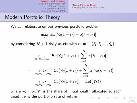
Modern Portfolio Theory
We can elaborate on our previous portfolio problem
maxa
E u[Y0(1 + rf ) + a(r − rf )]
by considering N > 1 risky assets with returns (r1, r2, ..., rN)
maxa1,a2,...,aN
E u[Y0(1 + rf ) +N∑i=1
ai (ri − rf )]
= maxw1,w2,...,wN
E u[Y0(1 + rf ) +N∑i=1
wiY0(ri − rf )]
= maxw1,w2,...,wN
E u[Y0(1 + rP)] = Eu((Y1))
where wi = ai/Y0 is the share of initial wealth allocated to eachasset. rP is the portfolio rate of return.
3 / 95
Modern portfolio theoryGains From Diversification
Efficient FrontierSeparation Theorem
Pros and Cons of MPT
Modern Portfolio TheoryJustifying Mean-Variance Utility
Modern Portfolio Theory
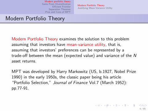
Modern Portfolio Theory examines the solution to this problemassuming that investors have mean-variance utility, that is,assuming that investors’ preferences can be represented by atrade-off between the mean (expected value) and variance of the Nasset returns.
MPT was developed by Harry Markowitz (US, b.1927, Nobel Prize1990) in the early 1950s, the classic paper being his article“Portfolio Selection,” Journal of Finance Vol.7 (March 1952):pp.77-91.
4 / 95
Modern portfolio theoryGains From Diversification
Efficient FrontierSeparation Theorem
Pros and Cons of MPT
Modern Portfolio TheoryJustifying Mean-Variance Utility
Modern Portfolio Theory: three steps
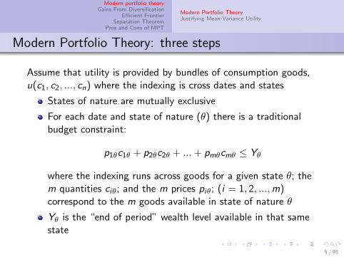
Assume that utility is provided by bundles of consumption goods,u(c1, c2, ..., cn) where the indexing is cross dates and states
States of nature are mutually exclusive
For each date and state of nature (θ) there is a traditionalbudget constraint:
p1θc1θ + p2θc2θ + ...+ pmθcmθ ≤ Yθ
where the indexing runs across goods for a given state θ; them quantities ciθ; and the m prices piθ; (i = 1, 2, ...,m)correspond to the m goods available in state of nature θ
Yθ is the “end of period” wealth level available in that samestate
5 / 95

Modern portfolio theoryGains From Diversification
Efficient FrontierSeparation Theorem
Pros and Cons of MPT
Modern Portfolio TheoryJustifying Mean-Variance Utility
Modern Portfolio Theory: three steps
MPT summarizes an individual’s decision problem as beingundertaken sequentially, in three steps.
1) The Consumption-Savings Decision: how to split periodzero income/wealth Y0 between current consumption now C0
and saving S0 for consumption in the future whereC0 + S0 = Y0
2) The Portfolio Problem: choose assets in which to investone’s savings so as to obtain a desired pattern of end-of-periodwealth across the various states of nature; this meansallocating (Y0 − C0) between a risk-free and N risky assets
3) The Consumption Choice: Given the realized state ofnature and the wealth level obtained, the choice ofconsumption bundles to maximize the utility function
Yθ = (Y0 − C0)[(1 + rf ) + ΣNi=1wi (riθ − rf )]
6 / 95
Modern portfolio theoryGains From Diversification
Efficient FrontierSeparation Theorem
Pros and Cons of MPT
Modern Portfolio TheoryJustifying Mean-Variance Utility
Modern Portfolio Theory: Backward Induction
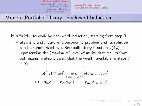
It is fruitful to work by backward induction, starting from step 3.
Step 3 is a standard microeconomic problem and its solutioncan be summarized by a Bernoulli utility function u(Yθ)representing the (maximum) level of utility that results fromoptimizing in step 3 given that the wealth available in state θis Yθ:
u(Yθ) ≡ def max(c1θ,...,cmθ)
u(c1θ, ..., cmθ)
s.t. p1θc1θ + p2θc2θ + ...+ pmθcmθ ≤ Yθ
7 / 95

Modern portfolio theoryGains From Diversification
Efficient FrontierSeparation Theorem
Pros and Cons of MPT
Modern Portfolio TheoryJustifying Mean-Variance Utility
Modern Portfolio Theory: Backward Induction
Maximizing Eu(Yθ) across all states of nature becomes theobjective of step 2:
max(w1,w2,...,wN)
Eu(Y ) = Σθπθu(Yθ)
The end-of-period wealth can be written as
Y = (Y0 − C0)(1 + rP)
rP = rf + ΣNi=1wi (ri − rf )
8 / 95
Modern portfolio theoryGains From Diversification
Efficient FrontierSeparation Theorem
Pros and Cons of MPT
Modern Portfolio TheoryJustifying Mean-Variance Utility
Modern Portfolio Theory: Backward Induction
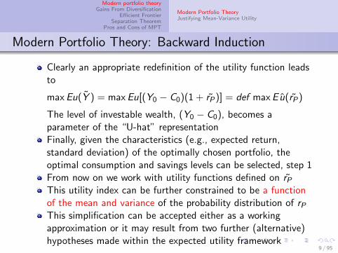
Clearly an appropriate redefinition of the utility function leadsto
max Eu(Y ) = max Eu[(Y0 − C0)(1 + rP)] = def max E u(rP)
The level of investable wealth, (Y0 − C0), becomes aparameter of the “U-hat” representationFinally, given the characteristics (e.g., expected return,standard deviation) of the optimally chosen portfolio, theoptimal consumption and savings levels can be selected, step 1From now on we work with utility functions defined on rPThis utility index can be further constrained to be a functionof the mean and variance of the probability distribution of rPThis simplification can be accepted either as a workingapproximation or it may result from two further (alternative)hypotheses made within the expected utility framework
9 / 95
Modern portfolio theoryGains From Diversification
Efficient FrontierSeparation Theorem
Pros and Cons of MPT
Modern Portfolio TheoryJustifying Mean-Variance Utility
Modern Portfolio Theory
The mean-variance utility hypothesis seemed natural at the timethe MPT first appeared, and it retains some intuitive appeal today.But viewed in the context of more recent developments in financialeconomics, particularly the development of vN-M expected utilitytheory, it now looks a bit peculiar.
A first question for us, therefore, is: Under what conditions willinvestors have preferences over the means and variances of assetreturns?
10 / 95

Modern portfolio theoryGains From Diversification
Efficient FrontierSeparation Theorem
Pros and Cons of MPT
Modern Portfolio TheoryJustifying Mean-Variance Utility
Justifying Mean-Variance Utility
In the exact case, we have two avenues:
A decision maker’s utility function is quadratic,
Asset returns are (jointly) normally distributed,
The main justification for using a mean-variance approximation isits tractability
Probability distributions are cumbersome to manipulate anddifficult to estimate empirically
Summarizing them by their first two moments is appealing
In the approximate case, using a simple Taylor seriesapproximation, one can also see that the mean and variance of anagent’s wealth distribution are critical to the determination of hisexpected utility for any distribution.
11 / 95

Modern portfolio theoryGains From Diversification
Efficient FrontierSeparation Theorem
Pros and Cons of MPT
Modern Portfolio TheoryJustifying Mean-Variance Utility
Justifying Mean-Variance Utility
If we start, as we did previously, by assuming an investor haspreferences over terminal wealth Y , potentially random because ofrandomness in the asset returns, described by a vN-M expectedutility function E [u(Y )]we can write
Y = E (Y ) + [Y − E (Y )]
and interpret the portfolio problem as a trade-off between theexpected payoff
E (Y )
and the size of the “bet”
[Y − E (Y )]
12 / 95
Modern portfolio theoryGains From Diversification
Efficient FrontierSeparation Theorem
Pros and Cons of MPT
Modern Portfolio TheoryJustifying Mean-Variance Utility
Justifying Mean-Variance Utility
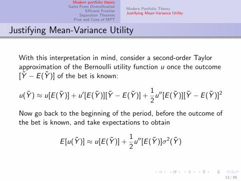
With this interpretation in mind, consider a second-order Taylorapproximation of the Bernoulli utility function u once the outcome[Y − E (Y )] of the bet is known:
u(Y ) ≈ u[E (Y )] + u′[E (Y )][Y − E (Y )] +1
2u′′[E (Y )][Y − E (Y )]2
Now go back to the beginning of the period, before the outcome ofthe bet is known, and take expectations to obtain
E [u(Y )] ≈ u[E (Y )] +1
2u′′[E (Y )]σ2(Y )
13 / 95
Modern portfolio theoryGains From Diversification
Efficient FrontierSeparation Theorem
Pros and Cons of MPT
Modern Portfolio TheoryJustifying Mean-Variance Utility
Justifying Mean-Variance Utility
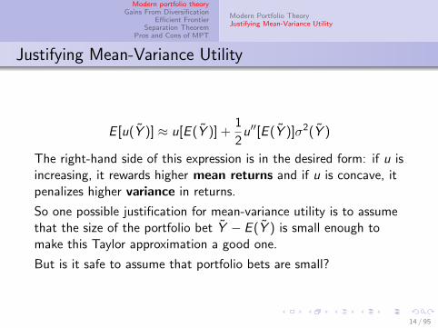
E [u(Y )] ≈ u[E (Y )] +1
2u′′[E (Y )]σ2(Y )
The right-hand side of this expression is in the desired form: if u isincreasing, it rewards higher mean returns and if u is concave, itpenalizes higher variance in returns.
So one possible justification for mean-variance utility is to assumethat the size of the portfolio bet Y − E (Y ) is small enough tomake this Taylor approximation a good one.
But is it safe to assume that portfolio bets are small?
14 / 95
Modern portfolio theoryGains From Diversification
Efficient FrontierSeparation Theorem
Pros and Cons of MPT
Modern Portfolio TheoryJustifying Mean-Variance Utility
Quadratic utility function
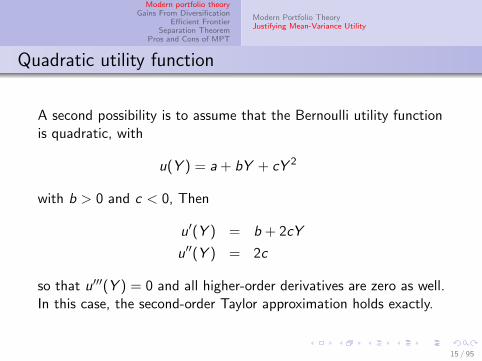
A second possibility is to assume that the Bernoulli utility functionis quadratic, with
u(Y ) = a + bY + cY 2
with b > 0 and c < 0, Then
u′(Y ) = b + 2cY
u′′(Y ) = 2c
so that u′′′(Y ) = 0 and all higher-order derivatives are zero as well.In this case, the second-order Taylor approximation holds exactly.
15 / 95

Modern portfolio theoryGains From Diversification
Efficient FrontierSeparation Theorem
Pros and Cons of MPT
Modern Portfolio TheoryJustifying Mean-Variance Utility
Quadratic utility function
Note, however, that for a quadratic utility function
RA(Y ) = −u′′(Y )
u′(Y )= − 2c
b + 2cY
which is increasing in Y .
Hence, quadratic utility has the undesirable implication that theamount of wealth allocated to risky investments declines whenwealth increases.
16 / 95
Modern portfolio theoryGains From Diversification
Efficient FrontierSeparation Theorem
Pros and Cons of MPT
Modern Portfolio TheoryJustifying Mean-Variance Utility
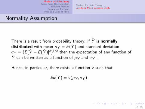
Normality Assumption
There is a result from probability theory: if Y is normallydistributed with mean µY = E (Y ) and standard deviationσY = (E [Y − E (Y )]2)1/2 then the expectation of any function ofY can be written as a function of µY and σY .
Hence, in particular, there exists a function v such that
Eu(Y ) = v(µY , σY )
17 / 95

Modern portfolio theoryGains From Diversification
Efficient FrontierSeparation Theorem
Pros and Cons of MPT
Modern Portfolio TheoryJustifying Mean-Variance Utility
Normality Assumption
The result follows from a more basic property of the normaldistribution: its location and shape is described completely by itsmean and variance.
18 / 95

Modern portfolio theoryGains From Diversification
Efficient FrontierSeparation Theorem
Pros and Cons of MPT
Modern Portfolio TheoryJustifying Mean-Variance Utility
Normality Assumption
If Y is normally distributed, there exists a function v such that
Eu(Y ) = v(µY , σY )
Moreover, if Y is normally distributed and
u is increasing, then v is increasing in µY
u is concave, then v is decreasing in σY
u is concave, then indifference curves defined over µY and σYare convex
19 / 95

Modern portfolio theoryGains From Diversification
Efficient FrontierSeparation Theorem
Pros and Cons of MPT
Modern Portfolio TheoryJustifying Mean-Variance Utility
Normality Assumption
Since µY is a “good” and σY is a “bad,” indifference curves slopeup. But if u is concave, these indifference curves will still beconvex.
20 / 95

Modern portfolio theoryGains From Diversification
Efficient FrontierSeparation Theorem
Pros and Cons of MPT
Modern Portfolio TheoryJustifying Mean-Variance Utility
Normality Assumption
Problems with the normality assumption:
limited liability instruments such as stocks can pay at worst anegative return of −100% (complete loss of the investment)
Returns on assets like options are highly non-normal.
While the normal is perfectly symmetric about its mean,high-frequency returns are frequently skewed to the right andindex returns appear skewed to the left
S(rit) = E [(rit − µi )
3
σ3i
]
Sample high-frequency return distributions for many assetsexhibit excess kurtosis or “fat tails
K (rit) = E [(rit − µi )
4
σ4i
]
21 / 95
Modern portfolio theoryGains From Diversification
Efficient FrontierSeparation Theorem
Pros and Cons of MPT
Modern Portfolio TheoryJustifying Mean-Variance Utility
Justifying Mean-Variance Utility
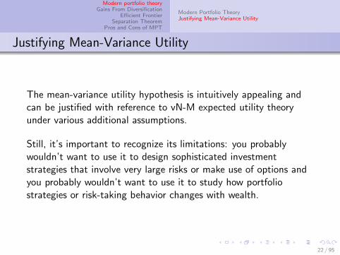
The mean-variance utility hypothesis is intuitively appealing andcan be justified with reference to vN-M expected utility theoryunder various additional assumptions.
Still, it’s important to recognize its limitations: you probablywouldn’t want to use it to design sophisticated investmentstrategies that involve very large risks or make use of options andyou probably wouldn’t want to use it to study how portfoliostrategies or risk-taking behavior changes with wealth.
22 / 95

Modern portfolio theoryGains From Diversification
Efficient FrontierSeparation Theorem
Pros and Cons of MPT
Two Risky AssetsPerfectly Correlated AssetsMean-Variance Frontier
Mean-Variance Dominance
In a mean-variance (M-V) framework, an investor’s wants tomaximize a function u(µr , σP)
She likes expected return (µr ) and dislikes standard deviation(σP)
Recall that portfolio A is said to exhibit mean-variancedominance over portfolio B if either
µA > µB and σA ≤ σB
µA ≥ µB and σA < σB
We can then define the efficient frontier as the locus of allnon-dominated portfolios in the mean-standard deviationspace
23 / 95

Modern portfolio theoryGains From Diversification
Efficient FrontierSeparation Theorem
Pros and Cons of MPT
Two Risky AssetsPerfectly Correlated AssetsMean-Variance Frontier
Mean-Variance Dominance
By definition, no (“rational”) mean-variance investor wouldchoose to hold a portfolio not located on the efficient frontier
The shape of the efficient frontier is of primary interest; let usexamine the efficient frontier in the two-asset case for avariety of possible asset return correlations
24 / 95

Modern portfolio theoryGains From Diversification
Efficient FrontierSeparation Theorem
Pros and Cons of MPT
Two Risky AssetsPerfectly Correlated AssetsMean-Variance Frontier
Two Risky Assets
One of the most important lessons that we can take from modernportfolio theory involves the gains from diversification.
To see where these gains come from, consider forming a portfoliofrom two risky assets:
r1, r2 = random returns
µ1, µ2 = expected returns
σ1, σ2 = standard deviations
Assume µ1 > µ2 and σ1 > σ2 to create a trade-off betweenexpected return and risk.
25 / 95

Modern portfolio theoryGains From Diversification
Efficient FrontierSeparation Theorem
Pros and Cons of MPT
Two Risky AssetsPerfectly Correlated AssetsMean-Variance Frontier
Two Risky Assets
If w is the fraction of initial wealth allocated to asset 1 and 1 − wis the fraction of initial wealth allocated to asset 2, the randomreturn rP on the portfolio is
rP = wr1 + (1 − w)r2
and the expected return µp on the portfolio is
µP = E [wr1 + (1 − w)r2]
= wE (r1) + (1 − w)E (r2)
= wµ1 + (1 − w)µ2
26 / 95
Modern portfolio theoryGains From Diversification
Efficient FrontierSeparation Theorem
Pros and Cons of MPT
Two Risky AssetsPerfectly Correlated AssetsMean-Variance Frontier
Two Risky Assets
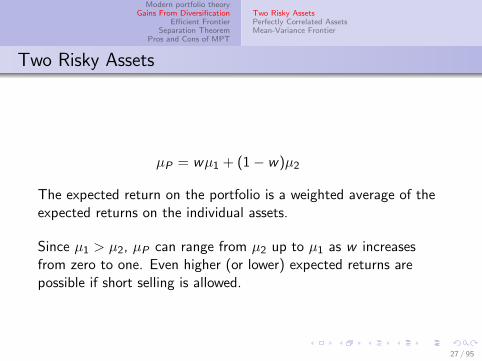
µP = wµ1 + (1 − w)µ2
The expected return on the portfolio is a weighted average of theexpected returns on the individual assets.
Since µ1 > µ2, µP can range from µ2 up to µ1 as w increasesfrom zero to one. Even higher (or lower) expected returns arepossible if short selling is allowed.
27 / 95

Modern portfolio theoryGains From Diversification
Efficient FrontierSeparation Theorem
Pros and Cons of MPT
Two Risky AssetsPerfectly Correlated AssetsMean-Variance Frontier
Two Risky Assets
We calculate the variance of the random portfolio return
rP = wr1 + (1 − w)r2
σ2P = E [(rP − µP)2]
= E ([wr1 + (1 − w)r2 − wµ1 − (1 − w)µ2]2)
= E ([w(r1 − µ1) + (1 − w)(r2 − µ2)]2)
= E [w 2(r1 − µ1)2 + (1 − w)2(r2 − µ2)2)
+ 2w(1 − w)(r1 − µ1)(r2 − µ2)]
= w 2E [(r1 − µ1)2] + (1 − w)2E [(r2 − µ2)2)]
+ 2w(1 − w)E [(r1 − µ1)(r2 − µ2)]
28 / 95

Modern portfolio theoryGains From Diversification
Efficient FrontierSeparation Theorem
Pros and Cons of MPT
Two Risky AssetsPerfectly Correlated AssetsMean-Variance Frontier
Covariance and correlation coefficient
In probability theory, the covariance between two random variablesX1 and X2 is defined as
σ(X1,X2) = E ([X1 − E (X1)][X2 − E (X2)])
and the correlation between X1 and X2 is defined as
ρ(X1,X2) =σ(X1,X2)
σ(X1)σ(X2)
29 / 95

Modern portfolio theoryGains From Diversification
Efficient FrontierSeparation Theorem
Pros and Cons of MPT
Two Risky AssetsPerfectly Correlated AssetsMean-Variance Frontier
Covariance and correlation coefficient
σ(X1,X2) = E ([X1 − E (X1)][X2 − E (X2)])
The covariance is
positive if X1 − E (X1) and X2 − E (X2) tend to have the samesign
negative if X1 − E (X1) and X2 − E (X2) tend to have oppositesigns
zero if X1 − E (X1) and X2 − E (X2) show no tendency to havethe same or opposite signs.
30 / 95

Modern portfolio theoryGains From Diversification
Efficient FrontierSeparation Theorem
Pros and Cons of MPT
Two Risky AssetsPerfectly Correlated AssetsMean-Variance Frontier
Covariance and correlation coefficient
Mathematically, therefore, the covariance
σ(X1,X2) = E ([X1 − E (X1)][X2 − E (X2)])
measures the extent to which the two random variables tend tomove together.
Economically, buying two assets with returns that are imperfectly,and especially, negatively correlated is like buying insurance: onereturn will be high when the other is low and vice versa, reducingthe overall risk of the portfolio.
31 / 95
Modern portfolio theoryGains From Diversification
Efficient FrontierSeparation Theorem
Pros and Cons of MPT
Two Risky AssetsPerfectly Correlated AssetsMean-Variance Frontier
Covariance and correlation coefficient
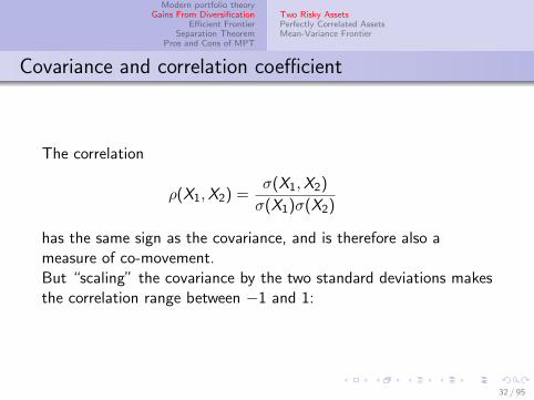
The correlation
ρ(X1,X2) =σ(X1,X2)
σ(X1)σ(X2)
has the same sign as the covariance, and is therefore also ameasure of co-movement.But “scaling” the covariance by the two standard deviations makesthe correlation range between −1 and 1:
32 / 95

Modern portfolio theoryGains From Diversification
Efficient FrontierSeparation Theorem
Pros and Cons of MPT
Two Risky AssetsPerfectly Correlated AssetsMean-Variance Frontier
Two Risky Assets
Hence
σ2P = w 2E [(r1 − µ1)2] + (1 − w)2E [(r2 − µ2)2)]
+ 2w(1 − w)E [(r1 − µ1)(r2 − µ2)]
= w 2σ21 + (1 − w)2σ2
2 + 2w(1 − w)σ12
= w 2σ21 + (1 − w)2σ2
2 + 2w(1 − w)σ1σ2ρ12
where
σ12 = the covariance between r1 and r2
ρ12 = the correlation between r1 and r2
33 / 95
Modern portfolio theoryGains From Diversification
Efficient FrontierSeparation Theorem
Pros and Cons of MPT
Two Risky AssetsPerfectly Correlated AssetsMean-Variance Frontier
Two Risky Assets
This is the source of the gains from diversification: the expectedportfolio return
µP = wµ1 + (1 − w)µ2
is a weighted average of the expected returns on the individualasset returns, but the standard deviation of the portfolio return
σP = [w 2σ21 + (1 − w)2σ2
2 + 2w(1 − w)σ1σ2ρ12]1/2
is not a weighted average of the standard deviations of the returnson the individual assets and can be reduced by choosing a mix ofassets (0 < w < 1) when ρ12 is less than one and, especially, whenρ12 is negative.
34 / 95

Modern portfolio theoryGains From Diversification
Efficient FrontierSeparation Theorem
Pros and Cons of MPT
Two Risky AssetsPerfectly Correlated AssetsMean-Variance Frontier
Mean Variance Portfolio(MVP)
σ2P = w 2σ2
1 + (1 − w)2σ22 + 2w(1 − w)σ1σ2ρ12
We can minimize the portfolio variance by setting the firstderivative equal to zero:
dσ2P
dw= 2wσ2
1 − 2σ22 + 2wσ2
2 + 2σ12 − 4wσ12 = 0
and solve for w∗
w∗ =σ2
2 − σ12
σ21 + σ2
2 − 2σ12
35 / 95
Modern portfolio theoryGains From Diversification
Efficient FrontierSeparation Theorem
Pros and Cons of MPT
Two Risky AssetsPerfectly Correlated AssetsMean-Variance Frontier
Two Risky Assets: ρ12 = 1
To see more specifically how this works, start with the case whereρ12 = 1 so that the individual asset returns are perfectly correlated.This is the one case in which there are no gains fromdiversification. With ρ12 = 1
µP = wµ1 + (1 − w)µ2
σP = [w 2σ21 + (1 − w)2σ2
2 + 2w(1 − w)σ1σ2ρ12]1/2
= [w 2σ21 + (1 − w)2σ2
2 + 2w(1 − w)σ1σ2]1/2
= ([wσ1 + (1 − w)σ2]2)1/2
= wσ1 + (1 − w)σ2
In this special case, the standard deviation of the return on theportfolio is a weighted average of the standard deviations of thereturns on the individual assets.
36 / 95
Modern portfolio theoryGains From Diversification
Efficient FrontierSeparation Theorem
Pros and Cons of MPT
Two Risky AssetsPerfectly Correlated AssetsMean-Variance Frontier
Two Risky Assets: ρ12 = 1
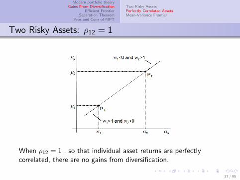
When ρ12 = 1 , so that individual asset returns are perfectlycorrelated, there are no gains from diversification.
37 / 95
Modern portfolio theoryGains From Diversification
Efficient FrontierSeparation Theorem
Pros and Cons of MPT
Two Risky AssetsPerfectly Correlated AssetsMean-Variance Frontier
Two Risky Assets: ρ12 = 1
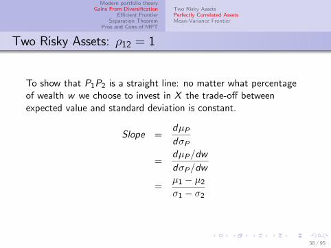
To show that P1P2 is a straight line: no matter what percentageof wealth w we choose to invest in X the trade-off betweenexpected value and standard deviation is constant.
Slope =dµPdσP
=dµP/dw
dσP/dw
=µ1 − µ2
σ1 − σ2
38 / 95
Modern portfolio theoryGains From Diversification
Efficient FrontierSeparation Theorem
Pros and Cons of MPT
Two Risky AssetsPerfectly Correlated AssetsMean-Variance Frontier
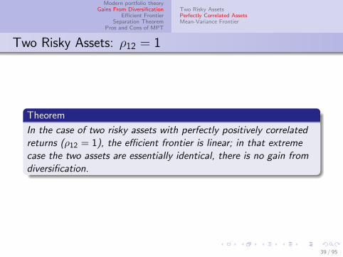
Two Risky Assets: ρ12 = 1
Theorem
In the case of two risky assets with perfectly positively correlatedreturns (ρ12 = 1), the efficient frontier is linear; in that extremecase the two assets are essentially identical, there is no gain fromdiversification.
39 / 95

Modern portfolio theoryGains From Diversification
Efficient FrontierSeparation Theorem
Pros and Cons of MPT
Two Risky AssetsPerfectly Correlated AssetsMean-Variance Frontier
Two Risky Assets: ρ12 = −1
Next, let’s consider the opposite extreme, in which ρ12 = −1 sothat the individual asset returns are perfectly, but negatively,correlated:
σP = [w 2σ21 + (1 − w)2σ2
2 + 2w(1 − w)σ1σ2ρ12]1/2
= [w 2σ21 + (1 − w)2σ2
2 − 2w(1 − w)σ1σ2]1/2
= ([wσ1 − (1 − w)σ2]2)1/2
= ±[wσ1 − (1 − w)σ2]
In this special case, the setting
w∗ =σ2
2 − σ12
σ21 + σ2
2 − 2σ12
=σ2
σ1 + σ2
creates a “synthetic” risk free portfolio(at w∗, σP = 0)!40 / 95

Modern portfolio theoryGains From Diversification
Efficient FrontierSeparation Theorem
Pros and Cons of MPT
Two Risky AssetsPerfectly Correlated AssetsMean-Variance Frontier
Two Risky Assets: ρ12 = −1
When ρ12 = −1 , so that individual asset returns are perfectly, butnegatively correlated, risk can be eliminated via diversification.
41 / 95

Modern portfolio theoryGains From Diversification
Efficient FrontierSeparation Theorem
Pros and Cons of MPT
Two Risky AssetsPerfectly Correlated AssetsMean-Variance Frontier
Two Risky Assets: ρ12 = 1
To show that P2Pmvp and PmvpP1 are linear: the slope is invariantto changes in percentage of an investor’s portfolio invested in X
Slope P2Pmvp =dµPdσP
=dµP/dw
dσP/dw
=µ1 − µ2
σ1 + σ2> 0
Slope PmvpP1 =dµPdσP
=dµP/dw
dσP/dw
=µ1 − µ2
−(σ1 + σ2)< 0
42 / 95

Modern portfolio theoryGains From Diversification
Efficient FrontierSeparation Theorem
Pros and Cons of MPT
Two Risky AssetsPerfectly Correlated AssetsMean-Variance Frontier
Two Risky Assets: ρ12 = −1
Theorem
If the two risky assets have returns that are perfectly negativelycorrelated (ρ12 = −1), the minimum variance portfolio is risk freewhile the frontier is linear.
If one of the two assets is risk free, then the efficient frontier is astraight line originating on the vertical axis at the level of therisk-free return.
43 / 95

Modern portfolio theoryGains From Diversification
Efficient FrontierSeparation Theorem
Pros and Cons of MPT
Two Risky AssetsPerfectly Correlated AssetsMean-Variance Frontier
Two Risky Assets
In the absence of a short sales restriction, the overall portfoliocan be made riskier than the riskiest among the existingassets; In other words, it can be made riskier than the onerisky asset and it must be that the efficient frontier isprojected to the right of the (µ2, σ2) point
44 / 95
Modern portfolio theoryGains From Diversification
Efficient FrontierSeparation Theorem
Pros and Cons of MPT
Two Risky AssetsPerfectly Correlated AssetsMean-Variance Frontier
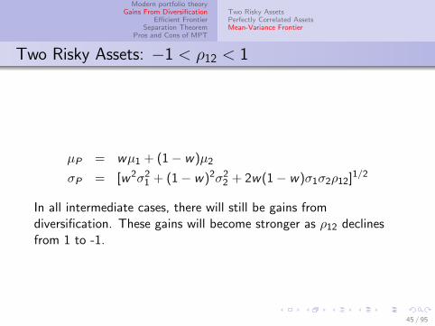
Two Risky Assets: −1 < ρ12 < 1
µP = wµ1 + (1 − w)µ2
σP = [w 2σ21 + (1 − w)2σ2
2 + 2w(1 − w)σ1σ2ρ12]1/2
In all intermediate cases, there will still be gains fromdiversification. These gains will become stronger as ρ12 declinesfrom 1 to -1.
45 / 95

Modern portfolio theoryGains From Diversification
Efficient FrontierSeparation Theorem
Pros and Cons of MPT
Two Risky AssetsPerfectly Correlated AssetsMean-Variance Frontier
Minimum Variance Frontier
Minimum Variance Frontier is the locus of risk and returncombinations offered by portfolios of risky assets that yield theminimum variance for a given rate of return.
In general, the MVF is convex, because it is bounded by thetriangle ABC.
46 / 95
Modern portfolio theoryGains From Diversification
Efficient FrontierSeparation Theorem
Pros and Cons of MPT
Two Risky AssetsPerfectly Correlated AssetsMean-Variance Frontier
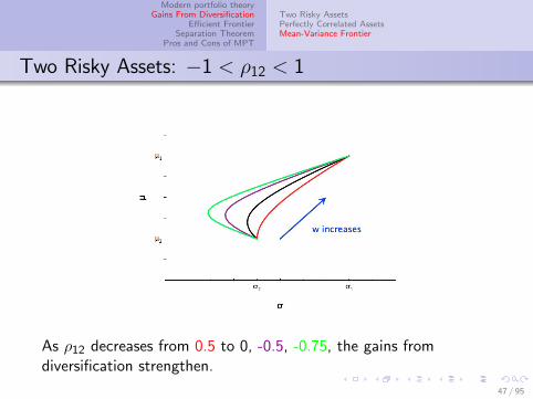
Two Risky Assets: −1 < ρ12 < 1
As ρ12 decreases from 0.5 to 0, -0.5, -0.75, the gains fromdiversification strengthen.
47 / 95

Modern portfolio theoryGains From Diversification
Efficient FrontierSeparation Theorem
Pros and Cons of MPT
Two Risky AssetsPerfectly Correlated AssetsMean-Variance Frontier
Two Risky Assets: −1 < ρ12 < 1
Theorem
In the case of two risky assets with imperfectly correlated returns(−1 < ρ12 < 1), the standard deviation of the portfolio isnecessarily smaller than it would be if the two component assetswere perfectly correlated:
σP < wσ1 + (1 − w)σ2
The smaller the correlation (further away from +1), the more tothe left is the MVF.
48 / 95

Modern portfolio theoryGains From Diversification
Efficient FrontierSeparation Theorem
Pros and Cons of MPT
Two Risky AssetsPerfectly Correlated AssetsMean-Variance Frontier
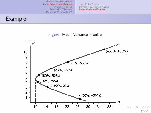
Example
Let R1 and R2 be the returns for two securities with E (R1) = 0.03and E (R2) = 0.08, Var(R1) = 0.02, Var(R2) = 0.05 andcov(R1,R2) = −0.01. Assuming that the two securities above arethe only investments available, plot the set of feasiblemean-variance combinations of return.
% in 1 % in 2 E (rP) var(rP) σP150 -50 0.5% 7.25% 26.93%100 0 3 2 14.1475 25 4.25 1.063 10.3150 50 5.5 1.25 11.1825 75 6.75 2.563 16.010 100 8 5 22.36-25 125 10.5 13.25 36.4
49 / 95
Modern portfolio theoryGains From Diversification
Efficient FrontierSeparation Theorem
Pros and Cons of MPT
Two Risky AssetsPerfectly Correlated AssetsMean-Variance Frontier
Example
Figure: Mean-Variance Frontier
50 / 95

Modern portfolio theoryGains From Diversification
Efficient FrontierSeparation Theorem
Pros and Cons of MPT
Two Risky AssetsPerfectly Correlated AssetsMean-Variance Frontier
Example
If we want to minimize risk, how much of our portfolio will weinvest in security 1?
w∗ =σ2
2 − σ12
σ21 + σ2
2 − 2σ12= 0.67
If we put two-thirds into asset 1, the portfolio’s standard deviationis
E (Rp) = 0.67 ∗ 0.03 + 0.33 ∗ 0.08 = 4.65%
var(RP) = 0.672 ∗ 0.02 + 0.332 ∗ 0.05 + 2 ∗ 0.67 ∗ 0.33 ∗ (−0.01)
= 0.01
The MVP is represented by the intersection of the dashed lines inthe figure.
51 / 95

Modern portfolio theoryGains From Diversification
Efficient FrontierSeparation Theorem
Pros and Cons of MPT
Three Risky AssetsMinimum Variance FrontierThe Efficient FrontierOptimal Portfolio Choice
Two Risky Assets and More?
µP = wµ1 + (1 − w)µ2
σP = [w 2σ21 + (1 − w)2σ2
2 + 2w(1 − w)σ1σ2ρ12]1/2
In the case with two risky assets, the choice of w simultaneouslydetermines µP and σP . Because a portfolio is also an asset fullydefined by its expected return, its standard deviation, and itscorrelation with other existing assets or portfolios; The previousanalysis with 2 assets is more general than it appears as it caneasily be repeated with one of the two assets being a portfolio.
But with more than two risky assets, the portfolio problem takeson an added dimension, since then we can ask: how can we selectw1,w2, ...,wN to minimize σP for any given choice of µP?
52 / 95

Modern portfolio theoryGains From Diversification
Efficient FrontierSeparation Theorem
Pros and Cons of MPT
Three Risky AssetsMinimum Variance FrontierThe Efficient FrontierOptimal Portfolio Choice
The Efficient Frontier
Consider two portfolios, A and B, with expected returns µA andµB and standard deviations σA and σB .
Recall that portfolio A is said to exhibit mean-variancedominance over portfolio B if either
µA > µB and σA ≤ σB
µA ≥ µB and σA < σB
Hence, choosing portfolio shares to minimize variance for a givenmean will allow us to characterize the efficient frontier: the set ofall portfolios that are not mean-variance dominated by any otherportfolio.This is a useful intermediate step in modern portfolio theory, sinceinvestors with mean-variance utility will only choose portfolios onthe efficient frontier.
53 / 95
Modern portfolio theoryGains From Diversification
Efficient FrontierSeparation Theorem
Pros and Cons of MPT
Three Risky AssetsMinimum Variance FrontierThe Efficient FrontierOptimal Portfolio Choice
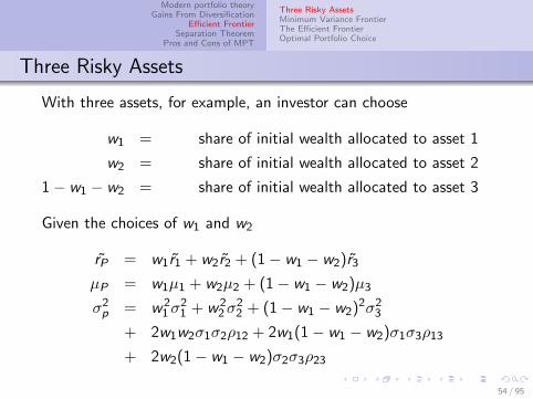
Three Risky Assets
With three assets, for example, an investor can choose
w1 = share of initial wealth allocated to asset 1
w2 = share of initial wealth allocated to asset 2
1 − w1 − w2 = share of initial wealth allocated to asset 3
Given the choices of w1 and w2
rP = w1r1 + w2r2 + (1 − w1 − w2)r3
µP = w1µ1 + w2µ2 + (1 − w1 − w2)µ3
σ2p = w 2
1σ21 + w 2
2σ22 + (1 − w1 − w2)2σ2
3
+ 2w1w2σ1σ2ρ12 + 2w1(1 − w1 − w2)σ1σ3ρ13
+ 2w2(1 − w1 − w2)σ2σ3ρ23
54 / 95

Modern portfolio theoryGains From Diversification
Efficient FrontierSeparation Theorem
Pros and Cons of MPT
Three Risky AssetsMinimum Variance FrontierThe Efficient FrontierOptimal Portfolio Choice
Three Risky Assets
Our problem is to solve
minw1,w2
σ2P
s.t. µP = µ
for a given value of µ.
But since we are more used to solving constrained maximizationproblems, consider the reformulated, but equivalent, problem:
maxw1,w2
−σ2P
s.t. µP = µ
55 / 95

Modern portfolio theoryGains From Diversification
Efficient FrontierSeparation Theorem
Pros and Cons of MPT
Three Risky AssetsMinimum Variance FrontierThe Efficient FrontierOptimal Portfolio Choice
Three Risky Assets
Set up the Lagrangian, using the expressions for µP and σPderived previously:
L = −[w 21σ
21 + w 2
2σ22 + (1 − w1 − w2)2σ2
3
+ 2w1w2σ1σ2ρ12 + 2w1(1 − w1 − w2)σ1σ3ρ13
+ 2w2(1 − w1 − w2)σ2σ3ρ23]
+ λ[w1µ1 + w2µ2 + (1 − w1 − w2)µ3 − µ]
56 / 95
Modern portfolio theoryGains From Diversification
Efficient FrontierSeparation Theorem
Pros and Cons of MPT
Three Risky AssetsMinimum Variance FrontierThe Efficient FrontierOptimal Portfolio Choice
Three Risky Assets
F.O.C. for w1
0 = −2w∗1 σ21 + 2(1 − w∗1 − w∗2 )σ2
3
− 2w∗2 σ1σ2ρ12 − 2(1 − w∗1 − w∗2 )σ1σ3ρ13
+ 2w∗1 σ1σ3ρ13 + 2w∗2 σ2σ3ρ23
+ λ∗µ1 − λ∗µ3
F.O.C. for w2
0 = −2w∗2 σ22 + 2(1 − w∗1 − w∗2 )σ2
3
− 2w∗1 σ1σ2ρ12 + 2w∗1 σ1σ3ρ13
− 2(1 − w∗1 − w∗2 )σ2σ3ρ23 + 2w∗2 σ2σ3ρ23
+ λ∗µ2 − λ∗µ3
B.C.
w∗1 µ1 + w∗2 µ2 + (1 − w∗1 − w∗2 )µ3 = µ
57 / 95
Modern portfolio theoryGains From Diversification
Efficient FrontierSeparation Theorem
Pros and Cons of MPT
Three Risky AssetsMinimum Variance FrontierThe Efficient FrontierOptimal Portfolio Choice
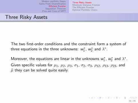
Three Risky Assets
The two first-order conditions and the constraint form a system ofthree equations in the three unknowns: w∗1 , w∗2 and λ∗.
Moreover, the equations are linear in the unknowns w∗1 , w∗2 and λ∗.
Given specific values for µ1, µ2, µ3, σ1, σ2, σ3, ρ12, ρ13, ρ23, andµ they can be solved quite easily.
58 / 95
Modern portfolio theoryGains From Diversification
Efficient FrontierSeparation Theorem
Pros and Cons of MPT
Three Risky AssetsMinimum Variance FrontierThe Efficient FrontierOptimal Portfolio Choice
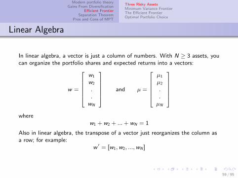
Linear Algebra
In linear algebra, a vector is just a column of numbers. With N ≥ 3 assets, youcan organize the portfolio shares and expected returns into a vectors:
w =
w1
w2
.
.wN
and µ =
µ1
µ2
.
.µN
where
w1 + w2 + ...+ wN = 1
Also in linear algebra, the transpose of a vector just reorganizes the column asa row; for example:
w ′ = [w1,w2, ...,wN ]
59 / 95

Modern portfolio theoryGains From Diversification
Efficient FrontierSeparation Theorem
Pros and Cons of MPT
Three Risky AssetsMinimum Variance FrontierThe Efficient FrontierOptimal Portfolio Choice
Linear Algebra
Meanwhile, the variances and covariances can be organized into amatrix — a collection of rows and columns:
Σ =
σ2
1 σ1σ2ρ12 ... σ1σNρ1N
σ1σ2ρ12 σ22 ... σ2σNρ2N
. . ... .
. . ... .σ1σNρ1N σ2σNρ2N ... σ2
N
60 / 95

Modern portfolio theoryGains From Diversification
Efficient FrontierSeparation Theorem
Pros and Cons of MPT
Three Risky AssetsMinimum Variance FrontierThe Efficient FrontierOptimal Portfolio Choice
Linear Algebra
Using the rules from linear algebra for multiplying vectors andmatrices, the expected return on any portfolio with shares in thevector w is
µ′w
and the variance of the random return on the portfolio is
w ′Σw
Hence, the problem of minimizing the variance for a given meancan be written compactly as
maxw
−w ′Σw s.t. µ′w = µ and l ′w = 1
where l is a vector of N ones.
61 / 95

Modern portfolio theoryGains From Diversification
Efficient FrontierSeparation Theorem
Pros and Cons of MPT
Three Risky AssetsMinimum Variance FrontierThe Efficient FrontierOptimal Portfolio Choice
Linear Algebra
maxw
−w ′Σw s.t. µ′w = µ and l ′w = 1
Problems of this form are called quadratic programming problemsand can be solved very quickly on a computer even when thenumber of assets N is large.
We can also add more constraints, such as wi ≥ 0, ruling out shortsales.
62 / 95

Modern portfolio theoryGains From Diversification
Efficient FrontierSeparation Theorem
Pros and Cons of MPT
Three Risky AssetsMinimum Variance FrontierThe Efficient FrontierOptimal Portfolio Choice
Three Risky Assets
Going back to the case with three assets, once the optimal sharesw∗1 and w∗2 have been found, the minimized standard deviation canbe computed using the general formula
σ2P = w 2
1σ21 + w 2
2σ22 + (1 − w1 − w2)2σ2
3
+ 2w1w2σ1σ2ρ12 + 2w1(1 − w1 − w2)σ1σ3ρ13
+ 2w2(1 − w1 − w2)σ2σ3ρ23
Doing this for various values of µ allows us to trace out theminimum variance frontier
63 / 95

Modern portfolio theoryGains From Diversification
Efficient FrontierSeparation Theorem
Pros and Cons of MPT
Three Risky AssetsMinimum Variance FrontierThe Efficient FrontierOptimal Portfolio Choice
Minimum Variance Frontier
Adding assets shifts the minimum variance frontier to the left, asopportunities for diversification are enhanced
64 / 95

Modern portfolio theoryGains From Diversification
Efficient FrontierSeparation Theorem
Pros and Cons of MPT
Three Risky AssetsMinimum Variance FrontierThe Efficient FrontierOptimal Portfolio Choice
Minimum Variance Frontier
However, the minimum variance frontier retains its sidewaysparabolic shape.
65 / 95

Modern portfolio theoryGains From Diversification
Efficient FrontierSeparation Theorem
Pros and Cons of MPT
Three Risky AssetsMinimum Variance FrontierThe Efficient FrontierOptimal Portfolio Choice
Minimum Variance Frontier
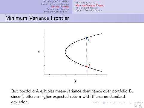
The minimum variance frontier traces out the minimizedvariance or standard deviation for each required mean return.
66 / 95
Modern portfolio theoryGains From Diversification
Efficient FrontierSeparation Theorem
Pros and Cons of MPT
Three Risky AssetsMinimum Variance FrontierThe Efficient FrontierOptimal Portfolio Choice
Minimum Variance Frontier
But portfolio A exhibits mean-variance dominance over portfolio B,since it offers a higher expected return with the same standarddeviation.
67 / 95
Modern portfolio theoryGains From Diversification
Efficient FrontierSeparation Theorem
Pros and Cons of MPT
Three Risky AssetsMinimum Variance FrontierThe Efficient FrontierOptimal Portfolio Choice
The Efficient Frontier
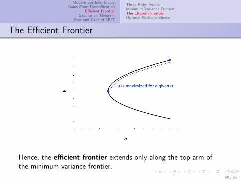
Hence, the efficient frontier extends only along the top arm ofthe minimum variance frontier.
68 / 95

Modern portfolio theoryGains From Diversification
Efficient FrontierSeparation Theorem
Pros and Cons of MPT
Three Risky AssetsMinimum Variance FrontierThe Efficient FrontierOptimal Portfolio Choice
The Efficient Frontier
Recall that either of two sets of assumptions will imply thatindifference curves in this µ− σ diagram slope upward and areconvex:
Investors have vN-M expected utility with quadratic Bernoulliutility functions
Asset returns are normally distributed and investors havevN-M expected utility with increasing and concave Bernoulliutility functions
69 / 95

Modern portfolio theoryGains From Diversification
Efficient FrontierSeparation Theorem
Pros and Cons of MPT
Three Risky AssetsMinimum Variance FrontierThe Efficient FrontierOptimal Portfolio Choice
The Optimal Portfolio Choice
Portfolios along U1 are mean-variance dominated by others.Portfolios along U3 are infeasible. Portfolio P∗, located where U2
is tangent to the efficient frontier, is optimal.70 / 95
Modern portfolio theoryGains From Diversification
Efficient FrontierSeparation Theorem
Pros and Cons of MPT
Three Risky AssetsMinimum Variance FrontierThe Efficient FrontierOptimal Portfolio Choice
The Optimal Portfolio Choice
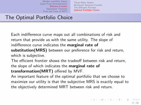
Each indifference curve maps out all combinations of risk andreturn that provide us with the same utility. The slope ofindifference curve indicates the marginal rate ofsubstitution(MRS) between our preference for risk and return,which is subjective.The efficient frontier shows the tradeoff between risk and return,the slope of which indicates the marginal rate oftransformation(MRT) offered by MVF.An important feature of the optimal portfolio that we choose tomaximize our utility is that the subjective MRS is exactly equal tothe objectively determined MRT between risk and return.
71 / 95

Modern portfolio theoryGains From Diversification
Efficient FrontierSeparation Theorem
Pros and Cons of MPT
Three Risky AssetsMinimum Variance FrontierThe Efficient FrontierOptimal Portfolio Choice
The Optimal Portfolio Choice
Investor B is less risk averse than investor A. Different investors face the sameassessment of the return and risk offered by risky assets, they may holddifferent portfolios. But all optimal portfolios are along the efficient frontier.
Thus, the mean-variance utility hypothesis built into Modern Portfolio Theory
implies that all investors choose optimal portfolios along the efficient frontier.
72 / 95

Modern portfolio theoryGains From Diversification
Efficient FrontierSeparation Theorem
Pros and Cons of MPT
One Risky asset & One Riskless assetSeparation Theorem
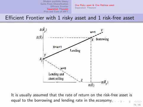
Efficient Frontier with 1 risky asset and 1 risk-free asset
So far, however, our analysis has assumed that there are only riskyassets. An additional, quite striking, result emerges when we add arisk free asset to the mix.
This implication was first noted by James Tobin (US, 1918-2002,Nobel Prize 1981) in his paper “Liquidity Preference as BehaviorTowards Risk,” Review of Economic Studies Vol.25 (February1958): pp.65-86.
73 / 95

Modern portfolio theoryGains From Diversification
Efficient FrontierSeparation Theorem
Pros and Cons of MPT
One Risky asset & One Riskless assetSeparation Theorem
Efficient Frontier with 1 risky asset and 1 risk-free asset
Consider, therefore, the larger portfolio formed when an investorallocates the fraction w of his or her initial wealth to a risky assetor to a smaller portfolio of risky assets and the remaining fraction1 − w to a risk free asset with return rf .
If the risky part of this portfolio has random return r , expectedreturn µr = E (r), and variance σ2
r = E [(r − µr )2] then the largerportfolio has random return rP = wr + (1 − w)rf with expectedreturn
µP = E [wr + (1 − w)rf ] = wµr + (1 − w)rf
and variance
σ2P = E [(rP − µP)2]
= E [wr + (1 − w)rf − wµr − (1 − w)rf ]2
= E [w(r − µr )]2 = w 2σ2r
74 / 95
Modern portfolio theoryGains From Diversification
Efficient FrontierSeparation Theorem
Pros and Cons of MPT
One Risky asset & One Riskless assetSeparation Theorem
Efficient Frontier with 1 risky asset and 1 risk-free asset
The expression for the portfolio’s variance
σ2P = w 2σ2
r
implies
σP = wσr
Hencew =
σPσr
Hence, with σr given, a larger share of wealth w allocated to riskyassets is associated with a higher standard deviation σP for thelarger portfolio.
75 / 95
Modern portfolio theoryGains From Diversification
Efficient FrontierSeparation Theorem
Pros and Cons of MPT
One Risky asset & One Riskless assetSeparation Theorem
Efficient Frontier with 1 risky asset and 1 risk-free asset
But the expression for the portfolio’s expected return
µP = wµr + (1 − w)rf
indicates that so long as µr > rf , a higher value of w will yield ahigher expected return as well.
What is the trade-off between risk σP and expected return µP ofthe mix of risky and riskless assets?
76 / 95

Modern portfolio theoryGains From Diversification
Efficient FrontierSeparation Theorem
Pros and Cons of MPT
One Risky asset & One Riskless assetSeparation Theorem
Efficient Frontier with 1 risky asset and 1 risk-free asset
To see, substitutew =
σPσr
intoµP = wµr + (1 − w)rf
to obtain
µP =σPσrµr + (1 − σP
σr)rf
= rf + (µr − rfσr
)σP
77 / 95
Modern portfolio theoryGains From Diversification
Efficient FrontierSeparation Theorem
Pros and Cons of MPT
One Risky asset & One Riskless assetSeparation Theorem
Efficient Frontier with 1 risky asset and 1 risk-free asset
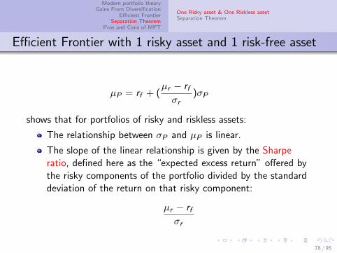
µP = rf + (µr − rfσr
)σP
shows that for portfolios of risky and riskless assets:
The relationship between σP and µP is linear.
The slope of the linear relationship is given by the Sharperatio, defined here as the “expected excess return” offered bythe risky components of the portfolio divided by the standarddeviation of the return on that risky component:
µr − rfσr
78 / 95
Modern portfolio theoryGains From Diversification
Efficient FrontierSeparation Theorem
Pros and Cons of MPT
One Risky asset & One Riskless assetSeparation Theorem
Efficient Frontier with 1 risky asset and 1 risk-free asset
It is usually assumed that the rate of return on the risk-free asset isequal to the borrowing and lending rate in the economy.
79 / 95
Modern portfolio theoryGains From Diversification
Efficient FrontierSeparation Theorem
Pros and Cons of MPT
One Risky asset & One Riskless assetSeparation Theorem
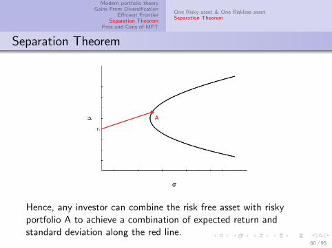
Separation Theorem
Hence, any investor can combine the risk free asset with riskyportfolio A to achieve a combination of expected return andstandard deviation along the red line.
80 / 95

Modern portfolio theoryGains From Diversification
Efficient FrontierSeparation Theorem
Pros and Cons of MPT
One Risky asset & One Riskless assetSeparation Theorem
Separation Theorem
However, any investor with mean-variance utility will prefer somecombination of the risk free asset and risky portfolio B to allcombinations of the risk free asset and risky portfolio A.
81 / 95

Modern portfolio theoryGains From Diversification
Efficient FrontierSeparation Theorem
Pros and Cons of MPT
One Risky asset & One Riskless assetSeparation Theorem
Separation Theorem
And all investors with mean-variance utility will prefer somecombination of the risk free asset and risky portfolio T to anyother portfolio.
82 / 95

Modern portfolio theoryGains From Diversification
Efficient FrontierSeparation Theorem
Pros and Cons of MPT
One Risky asset & One Riskless assetSeparation Theorem
Separation Theorem
Theorem
With N risky assets and a risk-free one, the efficient frontier is astraight line
We call T the tangency portfolio. As before, if we allow shortposition in the risk-free asset, the efficient frontier extends beyondT .
83 / 95

Modern portfolio theoryGains From Diversification
Efficient FrontierSeparation Theorem
Pros and Cons of MPT
One Risky asset & One Riskless assetSeparation Theorem
Separation Theorem
We now ask whether and how the MVF construction can be put toservice to inform actual portfolio practice: one result is surprising.
The optimal portfolio is naturally defined as that portfoliomaximizing the investor’s (mean-variance) utility; Thatportfolio for which he is able to reach the highest indifferencecurve in MV space;
Such curves will be increasing and convex from the origin;They are increasing because additional risk needs to becompensated by higher means; They are convex if and only ifthe investor is characterized by increasing absolute riskaversion (IARA), which is the case under MV preferences, aswe have claimed
84 / 95
Modern portfolio theoryGains From Diversification
Efficient FrontierSeparation Theorem
Pros and Cons of MPT
One Risky asset & One Riskless assetSeparation Theorem
Separation Theorem
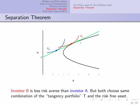
Investor B is less risk averse than investor A. But both choose samecombination of the “tangency portfolio” T and the risk free asset.
85 / 95

Modern portfolio theoryGains From Diversification
Efficient FrontierSeparation Theorem
Pros and Cons of MPT
One Risky asset & One Riskless assetSeparation Theorem
Separation Theorem
Note that the tangency portfolio T can be identified as theportfolio along the efficient frontier of risky assets that has thehighest Sharpe ratio.
86 / 95

Modern portfolio theoryGains From Diversification
Efficient FrontierSeparation Theorem
Pros and Cons of MPT
One Risky asset & One Riskless assetSeparation Theorem
Separation Theorem
Theorem
Any risk averse investor, independently of her risk aversion, willdiversify between a risky (tangency portfolio) fund and the risklessasset.
It is natural to realize that if there is a risk-free asset, then alltangency points must lie on the same efficient frontier,irrespective of the coefficient of risk aversion of each specificinvestor.
Let there be two investors sharing the same perceptions as toexpected returns, variances, and return correlations butdiffering in their willingness to take risks
87 / 95

Modern portfolio theoryGains From Diversification
Efficient FrontierSeparation Theorem
Pros and Cons of MPT
One Risky asset & One Riskless assetSeparation Theorem
Separation Theorem
Theorem
Any risk averse investor, independently of her risk aversion, willdiversify between a risky (tangency portfolio) fund and the risklessasset.
The relevant efficient frontier will be identical for these twoinvestors, although their optimal portfolios will be representedby different points on the same line
With differently shaped indifference curves the tangencypoints must differ.
88 / 95
Modern portfolio theoryGains From Diversification
Efficient FrontierSeparation Theorem
Pros and Cons of MPT
One Risky asset & One Riskless assetSeparation Theorem
Separation Theorem
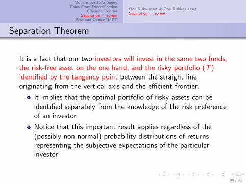
It is a fact that our two investors will invest in the same two funds,the risk-free asset on the one hand, and the risky portfolio (T )identified by the tangency point between the straight lineoriginating from the vertical axis and the efficient frontier.
It implies that the optimal portfolio of risky assets can beidentified separately from the knowledge of the risk preferenceof an investor
Notice that this important result applies regardless of the(possibly non normal) probability distributions of returnsrepresenting the subjective expectations of the particularinvestor
89 / 95

Modern portfolio theoryGains From Diversification
Efficient FrontierSeparation Theorem
Pros and Cons of MPT
One Risky asset & One Riskless assetSeparation Theorem
Separation Theorem
This is the two-fund theorem or separation theorem implied byModern Portfolio Theory.
Equity mutual fund managers can all focus on building the uniqueportfolio that lies along the efficient frontier of risky assets and hasthe highest Sharpe ratio.
Each individual investor can then tailor his or her own portfolio bychoosing the combination of the riskless assets and the riskymutual fund that best suits his or her own aversion to risk.
90 / 95

Modern portfolio theoryGains From Diversification
Efficient FrontierSeparation Theorem
Pros and Cons of MPT
Pros and Cons of MPT
We’ve already considered one shortcoming of the MPT: itsmean-variance utility hypothesis must rest on one of two morebasic assumptions.
Either utility must be quadratic or asset returns must be normal.
91 / 95

Modern portfolio theoryGains From Diversification
Efficient FrontierSeparation Theorem
Pros and Cons of MPT
Pros and Cons of MPT
A second problem involves the estimation or “calibration” of themodel’s parameters.
With N risky assets, the vector µ of expected returns contains Nelements and the matrix Σ of variances and covariances containsN(N + 1)/2 unique elements. When N = 100, for example, thereare 100 + (100 × 101)/2 = 5150 parameters to estimate!
And to use data from the past to estimate these parameters, onehas to assume that past averages and correlations are a reliableguide to the future.
92 / 95

Modern portfolio theoryGains From Diversification
Efficient FrontierSeparation Theorem
Pros and Cons of MPT
Pros and Cons of MPT
On the other hand, the MPT teaches us a very important lessonabout how individual assets with imperfectly, and especiallynegatively, correlated returns can be combined into a diversifiedportfolio to reduce risk.
And the MPT’s separation theorem suggests that a retirementsavings plan that allows participants to choose between a moneymarket mutual fund and a well-diversified equity fund is fullyoptimal under certain circumstances and perhaps close enough tooptimal more generally.
93 / 95
Modern portfolio theoryGains From Diversification
Efficient FrontierSeparation Theorem
Pros and Cons of MPT
Pros and Cons of MPT
Finally, our first equilibrium model of asset pricing, the CapitalAsset Pricing Model, builds directly on the foundations provided byModern Portfolio Theory.
94 / 95

Modern portfolio theoryGains From Diversification
Efficient FrontierSeparation Theorem
Pros and Cons of MPT
Summary
There is no contradiction between the way in which an economist looksat portfolio problems and what is typically done in practice in finance
We have defined mean-variance preferences and analyzed theirmicroeconomic foundations, which may be exact (quadratic utility, jointlynormally distributed returns) or approximated (Taylor)
We have built the minimum variance and mean-variance efficient frontiersfor a variety of cases, with and without constrains
We have examine how a risk-averse, IARA investor should be optimizingher portfolio with and without a riskless asset
The separation, or two-fund theorem emerged rather naturally from ourwork; we have discussed its implications for the asset managementindustry
We developed mean-variance closed-form asset allocation formulas
95 / 95