
Financial Economics: Capital Asset Pricing...
66
Financial Economics: Capital Asset Pricing Model Shuoxun Hellen Zhang WISE & SOE XIAMEN UNIVERSITY April, 2015 1 / 66
-
Upload
phunghuong -
Category
Documents
-
view
233 -
download
2
Transcript of Financial Economics: Capital Asset Pricing...

Financial Economics: Capital Asset Pricing
Model
Shuoxun Hellen Zhang
WISE & SOE
XIAMEN UNIVERSITY
April, 2015
1 / 66
Outline
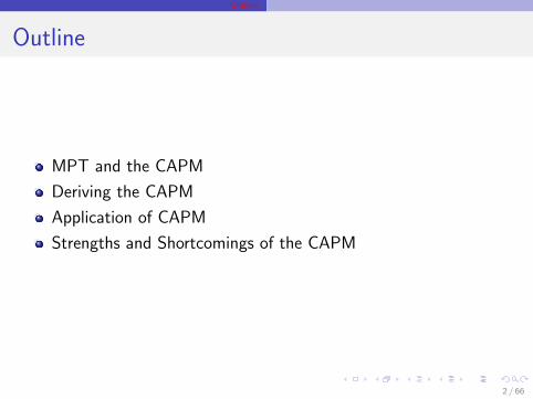
Outline
MPT and the CAPM
Deriving the CAPM
Application of CAPM
Strengths and Shortcomings of the CAPM
2 / 66
MPT and the CAPM
MPT and the CAPM
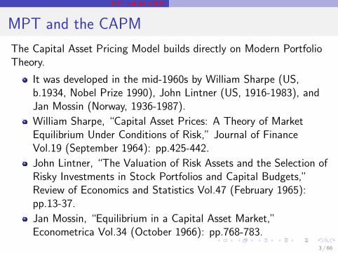
The Capital Asset Pricing Model builds directly on Modern PortfolioTheory.
It was developed in the mid-1960s by William Sharpe (US,b.1934, Nobel Prize 1990), John Lintner (US, 1916-1983), andJan Mossin (Norway, 1936-1987).
William Sharpe, “Capital Asset Prices: A Theory of MarketEquilibrium Under Conditions of Risk,” Journal of FinanceVol.19 (September 1964): pp.425-442.
John Lintner, “The Valuation of Risk Assets and the Selection ofRisky Investments in Stock Portfolios and Capital Budgets,”Review of Economics and Statistics Vol.47 (February 1965):pp.13-37.
Jan Mossin, “Equilibrium in a Capital Asset Market,”Econometrica Vol.34 (October 1966): pp.768-783.
3 / 66

MPT and the CAPM
MPT and the CAPM
Assumptions of the Capital Asset Pricing Model
Investors are risk-averse individuals who maximize the expectedutility of their end-of-period wealth
Investors are price-takers and have homogeneous expectationsabout asset returns that have a joint normal distribution
There exists a risk-free asset such that investors may borrow orlend unlimited amounts at the risk-free rate.
The quantities of assets are fixed. All assets are marketable andperfectly divisible.
Asset markets are frictionless and information is costless andsimultaneously available to all investors.
There are no market imperfections such as taxes, regulations, orrestrictions on short selling.
4 / 66

MPT and the CAPM
MPT and the CAPM
But whereas Modern Portfolio Theory is a theory describing thedemand for financial assets, the Capital Asset Pricing Model is atheory describing equilibrium in financial markets.
By making an additional assumption — namely, that supply equalsdemand in financial markets —the CAPM yields additionalimplications about the pricing of financial assets and risky cash flows.
5 / 66

MPT and the CAPM
MPT and the CAPM
Like MPT, the CAPM assumes that investors have mean-varianceutility and hence that either investors have quadratic Bernoulli utilityfunctions or that the random returns on risky assets are normallydistributed.
Thus, some of the same caveats that apply to MPT also apply to theCAPM.
For example, one might hesitate before applying the CAPM to priceoptions.
The traditional CAPM also assumes that there is a risk free asset aswell as a potentially large collection of risky assets.
Under these circumstances, as we’ve seen, all investors will hold somecombination of the riskless asset and the tangency portfolio: theefficient portfolio of risky assets with the highest Sharpe ratio.
6 / 66

MPT and the CAPM
MPT and the CAPM
But the CAPM goes further than the MPT by imposing anequilibrium condition.
Because there is no demand for risky financial assets except to theextent that they comprise the tangency portfolio, and because, inequilibrium, the supply of financial assets must equal demand, themarket portfolio consisting of all existing financial assets mustcoincide with the tangency portfolio.
In equilibrium, that is, “everyone” must “own the market.”
7 / 66

Deriving the CAPM Capital Market Line
CML, price of risk
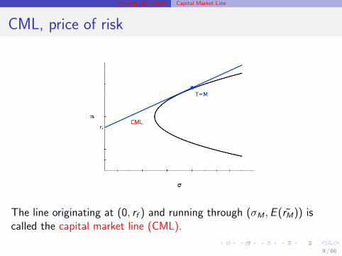
In the CAPM, equilibrium in financial markets requires the demandfor risky assets —the tangency portfolio— to coincide with thesupply of financial assets—the market portfolio.
The CAPM’s first implication is immediate: the market portfolio isefficient.
8 / 66
Deriving the CAPM Capital Market Line
CML, price of risk
The line originating at (0, rf ) and running through (σM ,E (r̃M)) iscalled the capital market line (CML).
9 / 66

Deriving the CAPM Capital Market Line
CML, price of risk
Endowed with point A, we always have two choices available when there is a
capital market: moving along the MVF or moving along CML by borrowing and
lending. First move to B where MRS=MRT of the MVF, and U1 increases to U2;
Then we can better off by moving to M and borrowing to reach C, utility
increases to U3.10 / 66

Deriving the CAPM Capital Market Line
CML, price of risk
Nearly everyone is better off in a world with capital markets.
Two-fund theorem obtains.
In equilibrium, the MRS is the same for all individuals, regardlessof their subjective attitude to risk.
11 / 66

Deriving the CAPM Capital Market Line
CML, price of risk
Hence, it also follows that all individually optimal portfolios arelocated along the CML and are formed as combinations of the riskfree asset and the market portfolio.
12 / 66

Deriving the CAPM Capital Market Line
CML, price of risk
Recall that the trade-off between the standard deviation andexpected return of any portfolio combining the riskless asset and thetangency portfolio is described by the linear relationship
E (r̃P) = rf + [E (r̃T )− rf
σT]σP
Since the CAPM implies that the tangency and market portfolioscoincide, the formula for the Capital Market Line is likewise
E (r̃P) = rf + [E (r̃M)− rf
σM]σP
13 / 66

Deriving the CAPM Capital Market Line
CML, price of risk
And since all individually optimal portfolios are located along theCML, the equation
E (r̃P) = rf + [E (r̃M)− rf
σM]σP
implies that the market portfolio’s Sharpe ratio
E (r̃M)− rfσM
measures the equilibrium price of risk: the expected return thateach investor gives up when he or she adjusts his or her totalportfolio to reduce risk, i.e., it shows how much must be given up inexpected portfolio rate of return in order to reduce standard deviationby one unit.
14 / 66

Deriving the CAPM Motivation of CAPM
Motivation
Capital Asset Pricing Model shows what determines prices ofindividual assets.
First motivation: Covariance is important.
Comparing alternative portfolios, when only one of them can bechosen, have assumed variances of rates of return are therelevant measure of risk.
But for individual assets, which can be combined in portfolios,the relevant measure turns out to be a covariance with otherrates of return.
15 / 66

Deriving the CAPM Motivation of CAPM
Motivation
Consider making an equally weighted portfolio of n assets, i.e., withall wj = 1/n. Assume that among the rates of return, one has themaximum variance, σ2
max . Then
limn→∞
σ2p = σ̄ij
the average covariance between rates of return, and
limn→∞
∂σ2p
∂wi= 2σ̄ij
16 / 66

Deriving the CAPM Motivation of CAPM
Proof
Observe thatσ2p = Σn
i=1Σnj=1wiwjσij
An equally weighted portfolio has
σ2p =
1
n2Σn
i=1Σnj=1σij =
1
n2Σn
i=1σ2i +
1
n2Σn
i=1Σj 6=iσij
Observe that the first term satisfies
1
n2Σn
i=1σ2i <
1
n2∗ n ∗ σ2
max → 0⇐ n→∞
The second term satisfies
1
n2Σn
i=1Σj 6=iσij =n2 − n
n2σ̄ij → σ̄ij ⇐ n→∞
which proves the first result.17 / 66

Deriving the CAPM Motivation of CAPM
Proof
Observe next that for any portfolio
∂σ2p
∂wi= 2wiσ
2i + 2Σj 6=iwjσij
Evaluated where all wi = 1/n, this becomes
2σ2i
n+ 2
n − 1
nσ̄ij → 2σ̄ij ⇐ n→∞
18 / 66

Deriving the CAPM Derivation of CAPM formula
Deriving the CAPM
Consider an equilibrium, everyone holds combination of risk free assetand market portfolio. Next, let’s consider an arbitrary asset — “assetj” — with random return r̃j , expected return E (r̃j), and standarddeviation σj .(Possible, even though M already contains j .))
MPT would take E (r̃j) and σj as “data”—that is, as given.
The CAPM again goes further and asks: if asset j is to be demandedby investors with mean-variance utility, what restrictions must E (r̃j)and σj satisfy?
19 / 66

Deriving the CAPM Derivation of CAPM formula
Deriving the CAPM
To answer this question, consider an investor who takes the portionof his or her initial wealth that he or she allocates to risky assets anddivides it further: using the fraction w to purchase asset j and theremaining fraction 1− w to buy the market portfolio.
Note that since the market portfolio already includes some of asset j ,choosing w > 0 really means that the investor “overweights” asset jin his or her own portfolio. Conversely, choosing w < 0 means thatthe investor “underweights” asset j in his or her own portfolio.
20 / 66

Deriving the CAPM Derivation of CAPM formula
Deriving the CAPM
Based on our previous analysis, we know that this investor’s portfolioof risky assets now has random return
r̃P = wr̃j + (1− w)r̃M
expected return
E (r̃P) = wE (r̃j) + (1− w)E (r̃M)
and variance
σ2P = w 2σ2
j + (1− w)2σ2M + 2w(1− w)σjM
where σjM is the covariance between r̃j and r̃M . We can use theseformulas to trace out how σP and E (r̃P) vary as w changes.
21 / 66

Deriving the CAPM Derivation of CAPM formula
Deriving the CAPM
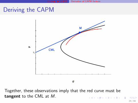
The red curve traces out how σP and E (r̃P) vary as w changes, thatis, as asset j gets underweighted or overweighted relative to themarket portfolio.
The red curve passes through M , since when w = 0 the new portfoliocoincides with the market portfolio. For all other values of w,however, the red curve must lie below the CML.
22 / 66

Deriving the CAPM Derivation of CAPM formula
Deriving the CAPM
Otherwise, a portfolio along the CML would be dominated inmean-variance by the new portfolio. Financial markets would nolonger be in equilibrium, since some investors would no longer bewilling to hold the market portfolio.
23 / 66
Deriving the CAPM Derivation of CAPM formula
Deriving the CAPM
Together, these observations imply that the red curve must betangent to the CML at M .
24 / 66

Deriving the CAPM Derivation of CAPM formula
Deriving the CAPM
Tangent means equal in slope.
We already know that the slope of the Capital Market Line is
E (r̃M)− rfσM
But what is the slope of the red curve?
25 / 66

Deriving the CAPM Derivation of CAPM formula
Deriving the CAPM
Let f (σP) be the function defined by E (r̃P) = f (σP) and thereforedescribing the red curve.
26 / 66

Deriving the CAPM Derivation of CAPM formula
Deriving the CAPM
Next, define the functions g(w) and h(w) by
g(w) = wE (r̃j) + (1− w)E (r̃M)
h(w) = [w 2σ2j + (1− w)2σ2
M + 2w(1− w)σjM ]1/2
so that
E (r̃P) = g(w)
σP = h(w)
27 / 66

Deriving the CAPM Derivation of CAPM formula
Deriving the CAPM
Substitute
E (r̃P) = g(w)
σP = h(w)
intoE (r̃P) = f (σP)
theng(w) = f (h(w))
and use the chain rule to compute
g ′(w) = f ′(h(w))h′(w) = f ′(σP)h′(w)
28 / 66

Deriving the CAPM Derivation of CAPM formula
Deriving the CAPM
Let f (σP) be the function defined by E (r̃P) = f (σP) and thereforedescribing the red curve. Then f ′(σP) is the slope of the curve.Hence, to compute f ′(σP), we can rearrange
g ′(w) = f ′(h(w))h′(w) = f ′(σP)h′(w)
and get
f ′(σP) =g ′(w)
h′(w)
and compute g ′(w) and h′(w) from the formulas we know
g(w) = wE (r̃j) + (1− w)E (r̃M)
impliesg ′(w) = E (r̃j)− E (r̃M)
29 / 66

Deriving the CAPM Derivation of CAPM formula
Deriving the CAPM
h(w) = [w 2σ2j + (1− w)2σ2
M + 2w(1− w)σjM ]1/2
implies
h′(w) =1
2(
2wσ2j − 2(1− w)σ2
M + 2(1− 2w)σjM
[w 2σ2j + (1− w)2σ2
M + 2w(1− w)σjM ]1/2)
=wσ2
j − (1− w)σ2M + (1− 2w)σjM
[w 2σ2j + (1− w)2σ2
M + 2w(1− w)σjM ]1/2
so
f ′(σP) =g ′(w)
h′(w)
= [E (r̃j)− E (r̃M)]
∗[w 2σ2
j + (1− w)2σ2M + 2w(1− w)σjM ]1/2
wσ2j − (1− w)σ2
M + (1− 2w)σjM30 / 66

Deriving the CAPM Derivation of CAPM formula
Deriving the CAPM
The red curve is tangent to the CML at M. Hence f ′(σP) equals theslope of the CML when w = 0
31 / 66

Deriving the CAPM Derivation of CAPM formula
Deriving the CAPM
When w = 0
f ′(σP) = [E (r̃j)− E (r̃M)] ∗[w 2σ2
j + (1− w)2σ2M + 2w(1− w)σjM ]1/2
wσ2j − (1− w)σ2
M + (1− 2w)σjM
implies
f ′(σP) =[E (r̃j)− E (r̃M)]σM
σjM − σ2M
Meanwhile, we know that the slope of the CML is
E (r̃M)− rfσM
32 / 66

Deriving the CAPM Derivation of CAPM formula
Deriving the CAPM
The tangency of the red curve with the CML at M therefore requires
[E (r̃j)− E (r̃M)]σMσjM − σ2
M
=E (r̃M)− rf
σM
E (r̃j)− E (r̃M) =[E (r̃M)− rf ][σjM − σ2
M ]
σ2M
E (r̃j)− E (r̃M) =σjMσ2M
[E (r̃M)− rf ]− [E (r̃M)− rf ]
E (r̃j) = rf +σjMσ2M
[E (r̃M)− rf ]
33 / 66
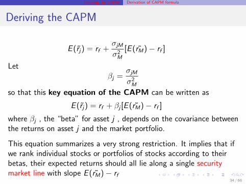
Deriving the CAPM Derivation of CAPM formula
Deriving the CAPM
E (r̃j) = rf +σjMσ2M
[E (r̃M)− rf ]
Letβj =
σjMσ2M
so that this key equation of the CAPM can be written as
E (r̃j) = rf + βj [E (r̃M)− rf ]
where βj , the “beta” for asset j , depends on the covariance betweenthe returns on asset j and the market portfolio.
This equation summarizes a very strong restriction. It implies that ifwe rank individual stocks or portfolios of stocks according to theirbetas, their expected returns should all lie along a single securitymarket line with slope E (r̃M)− rf
34 / 66

Deriving the CAPM Derivation of CAPM formula
Deriving the CAPM
According to the CAPM, all assets and portfolios of assets lie along asingle security market line. Those with higher betas have higherexpected returns.
35 / 66

Deriving the CAPM Derivation of CAPM formula
Security market line
Observe βM = 1
Observe βj = ρjMσj/σM
May have σj > σM , and ρjM close to 1;Thus possible to haveβj > 1 for some assets
May also have σjM < 0, βj < 0, not very common in practice;Such assets contribute to reducing σM (when included in M).
36 / 66

Deriving the CAPM Derivation of CAPM formula
Security market line
Any portfolio of m securities locate on the SML. Show for m = 2
µp = wµi + (1− w)µj
= w [rf + βi(µM − rf )] + (1− w)[rf + βj(µM − rf )])
= rf + [wβi + (1− w)βj ](µM − rf )
= rf + [wcov(r̃i , r̃M)
σ2M
+ (1− w)cov(r̃j , r̃M)
σ2M
](µM − rf )
= rf +cov(wr̃i + (1− w)r̃j , r̃M)
σ2M
(µM − rf )
= rf +cov(r̃p, r̃M)
σ2M
(µM − rf )
= rf + βp(µM − rf )
βp is a value-weighted average of βi and βj .37 / 66

Deriving the CAPM Derivation of CAPM formula
CML V.S. SML
Capital Market Line
Efficient set given 1 risk free and n risky assets.
Relevant for choice between alternative portfolios.
Drawn in (σp, µp) diagram.
A ray starting at (0, rf ) in that diagram.
Security market line
Location of all traded assets in equilibrium.
Also location of any portfolio of these assets.
Not relevant for choice between assets which are already traded,so that equilibrium prices are observable.
But relevant if equilibrium price at t = 0 is unknown.
Drawn in (βj , µj) diagram.
A line through (0, rf ) in that diagram38 / 66
Deriving the CAPM Interpretation
Interpretation
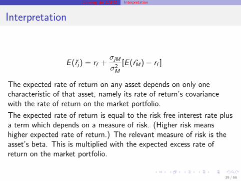
E (r̃j) = rf +σjMσ2M
[E (r̃M)− rf ]
The expected rate of return on any asset depends on only onecharacteristic of that asset, namely its rate of return’s covariancewith the rate of return on the market portfolio.
The expected rate of return is equal to the risk free interest rate plusa term which depends on a measure of risk. (Higher risk meanshigher expected rate of return.) The relevant measure of risk is theasset’s beta. This is multiplied with the expected excess rate ofreturn on the market portfolio.
39 / 66
Deriving the CAPM Interpretation
Interpretation
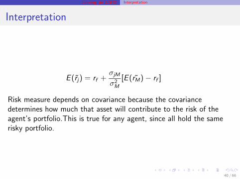
E (r̃j) = rf +σjMσ2M
[E (r̃M)− rf ]
Risk measure depends on covariance because the covariancedetermines how much that asset will contribute to the risk of theagent’s portfolio.This is true for any agent, since all hold the samerisky portfolio.
40 / 66

Deriving the CAPM Interpretation
Interpretation
There are two complementary ways of interpreting this result.
Both bring us back to the theme of diversification emphasized byMPT.
Both take us a step further, by emphasizing as well the idea ofaggregate risk, which cannot be “diversified away,” and idiosyncraticrisk, which can be diversified away.
41 / 66

Deriving the CAPM first interpretation
Aggregate risk & idiosyncratic risk
The first approach uses the CAPM equation in its original form
E (r̃j) = rf +σjMσ2M
[E (r̃M)− rf ]
together with the definition of correlation, which implies
ρjM =σjMσjσM
Then the CAPM relationship
E (r̃j) = rf + [E (r̃M)− rf
σM]ρjMσj
42 / 66

Deriving the CAPM first interpretation
Aggregate risk & idiosyncratic risk
E (r̃j) = rf + [E (r̃M)− rf
σM]ρjMσj
The term inside brackets is the equilibrium price of risk.
And since the correlation lies between −1 and 1, the term ρjMσj ,satisfying
ρjMσj ≤ σj
represents the “portion” of the total risk σj in asset j that iscorrelated with the market return.
43 / 66

Deriving the CAPM first interpretation
Aggregate risk & idiosyncratic risk
E (r̃j) = rf + [E (r̃M)− rf
σM]ρjMσj
The idiosyncratic risk in asset j , that is, the portion that isuncorrelated with the market return, can be diversified away byholding the market portfolio.Since this risk can be freely shed through diversification, it is not“priced.”
Hence, according to the CAPM, risk in asset j is priced only to theextent that it takes the form of aggregate risk that, because it iscorrelated with the market portfolio, cannot be diversified away.
44 / 66

Deriving the CAPM first interpretation
Aggregate risk & idiosyncratic risk
E (r̃j) = rf + [E (r̃M)− rf
σM]ρjMσj
Thus, according to the CAPM:
Only assets with random returns that are positively correlatedwith the market return earn expected returns above the risk freerate. They must, in order to induce investors to take on moreaggregate risk.
Assets with returns that are uncorrelated with the market returnhave expected returns equal to the risk free rate, since their riskcan be completely diversified away.
45 / 66

Deriving the CAPM first interpretation
Aggregate risk & idiosyncratic risk
E (r̃j) = rf + [E (r̃M)− rf
σM]ρjMσj
Thus, according to the CAPM:
Assets with negative betas —that is, with random returns thatare negatively correlated with the market return— have expectedreturns below the risk free rate! For these assets, E (r̃j)− rf < 0is like an “insurance premium” that investors will pay in order toinsulate themselves from aggregate risk.
46 / 66

Deriving the CAPM Second interpretation
Statistical interpretation
The second approach to interpreting the CAPM uses
E (r̃j) = rf + βj [E (r̃M)− rf ]
together with the definition of
βj =σjMσ2M
47 / 66

Deriving the CAPM Second interpretation
Statistical interpretation
Consider a statistical regression of the random return r̃j on asset j ona constant and the market return r̃M
r̃j = α + βj r̃M + εj
This regression breaks the variance of r̃j down into two “orthogonal”(uncorrelated) components:
The component βj r̃M that is systematically related to variationin the market return.
The component εj that is not.
Do you remember the formula for βj , the slope coefficient in a linearregression? It is
βj =σjMσ2M
the same “beta” as in the CAPM!48 / 66

Deriving the CAPM Second interpretation
Statistical interpretation
r̃j = α + βj r̃M + εj
But this is not an accident: to the contrary, it restates the conclusionthat, according to the CAPM, risk in an individual asset is priced—and thereby reflected in a higher expected return—only to the extentthat it is correlated with the market return.
49 / 66

Deriving the CAPM Second interpretation
Statistical interpretation
r̃j = α + βj r̃M + εj
E (r̃j) = rf + βj [E (r̃M)− rf ]
the CAPM equation implies E (εj) = 0 and
cov(εj , r̃M) = cov(r̃j − α− βj r̃M , r̃M)
= cov(r̃j , r̃M)− βjvar(r̃M)
= σjM − βjσ2M = 0
50 / 66

Deriving the CAPM Second interpretation
Statistical interpretation
This allows us to split σ2j in two parts:
var(r̃j) ≡ σ2j = β2
j σ2M + σ2
εj= βjσjM + σ2
εj
First term is the aggregate risk. This is reflected in the marketvaluation. Second term is the unsystematic risk or idiosyncratic risk.As we have seen, it is not reflected in market valuation.The sum of the two called total risk or variance risk. This is relevantfor portfolios, evaluated for being the total wealth of someone, butnot for individual securities, to be combined with other securities inportfolios.
51 / 66

Deriving the CAPM Second interpretation
Statistical interpretation
r̃j = α + βj r̃M + εj
For a portfolio: Variance is the relevant risk measure.
For each security: Covariance with r̃M is relevant. Becausecovariance measures contribution to portfolio variance.
Generally: Covariance with each agent’s marginal utility; butwith mean-variance preferences: Covariance with agent’s wealth.In equilibrium, all have same risky portfolio (composition); Thuscovariance with r̃M is relevant for everyone.
52 / 66

Application of CAPM Valuing Risky Cash Flows
Valuing Risky Cash Flows
We can also use the CAPM to value risky cash flows.
Let C̃t+1 denote a random payoff to be received at time t + 1 (“oneperiod from now”) and let PC
t denote its price at time t (“today.”)
If C̃t+1 was known in advance, that is, if the payoff were riskless, wecould find its value by discounting it at the risk free rate:
PCt =
C̃t+1
1 + rf
53 / 66
Application of CAPM Valuing Risky Cash Flows
Valuing Risky Cash Flows
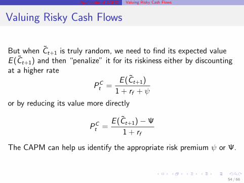
But when C̃t+1 is truly random, we need to find its expected valueE (C̃t+1) and then “penalize” it for its riskiness either by discountingat a higher rate
PCt =
E (C̃t+1)
1 + rf + ψ
or by reducing its value more directly
PCt =
E (C̃t+1)−Ψ
1 + rf
The CAPM can help us identify the appropriate risk premium ψ or Ψ.
54 / 66

Application of CAPM Valuing Risky Cash Flows
Valuing Risky Cash Flows
Our previous analysis suggests that, broadly speaking, the riskpremium implied by the CAPM will somehow depend on the extentto which the random payoff C̃t+1 is correlated with the return on themarket portfolio.
To apply the CAPM to this valuation problem, we can start byobserving that with price PC
t today and random payoff C̃t+1 oneperiod from now, the return on this asset or investment project isdefined by
1 + r̃C =C̃t+1
PCt
or
r̃C =C̃t+1 − PC
t
PCt
where the notation r̃C emphasizes that this return, like the futurecash flow itself, is risky. 55 / 66

Application of CAPM Valuing Risky Cash Flows
Valuing Risky Cash Flows
Now the CAPM implies that the expected return E (r̃C ) must satisfy
E (r̃C ) = rf + βC [E (r̃M)− rf ]
where the project’s beta depends on the covariance of its return withthe market return:
βC =σCMσ2M
This is what takes skill: with an existing asset, one can use data onthe past correlation between its return and the market return toestimate beta. With a totally new project that is just being planned,a combination of experience, creativity, and hard work is often neededto choose the right value for βC .
56 / 66

Application of CAPM Valuing Risky Cash Flows
Valuing Risky Cash Flows
But once a value for βC is determined, we can use
E (r̃C ) = rf + βC [E (r̃M)− rf ]
together with the definition of the return itself
r̃C =C̃t+1
PCt
− 1
to write
E (C̃t+1
PCt
− 1) = rf + βC [E (r̃M)− rf ]
which implies
(1
PCt
)E (C̃t+1) = 1 + rf + βC [E (r̃M)− rf ]
PCt =
E (C̃t+1)
1 + rf + βC [E (r̃M)− rf ]57 / 66

Application of CAPM Valuing Risky Cash Flows
Valuing Risky Cash Flows
PCt =
E (C̃t+1)
1 + rf + βC [E (r̃M)− rf ]
Right-hand side is “expected present value”, withRisk-adjusted discount rate(RADR). Risk-adjustment againdepends on (E (r̃M)− rf )/σ2
M and covariance.
E (r̃C ) = rf + βC [E (r̃M)− rf ]
the CAPM implies a risk premium of
ψ = βC [E (r̃M)− rf ]
depends critically on the covariance between the return on the riskyproject and the return on the market portfolio.
58 / 66

Application of CAPM Valuing Risky Cash Flows
Valuing Risky Cash Flows
Alternatively,
(1
PCt
)E (C̃t+1) = 1 + rf + βC [E (r̃M)− rf ]
can be rewritten as
PCt =
E (C̃t+1)− PCt βC [E (r̃M)− rf ]
1 + rf
indicating that the CAPM also implies
Ψ = PCt βC [E (r̃M)− rf ]
which, again as expected, depends critically on the covariancebetween the return on the risky project and the return on the marketportfolio.
59 / 66

Application of CAPM Valuing Risky Cash Flows
Valuing Risky Cash Flows
PCt =
E (C̃t+1)− PCt βC [E (r̃M)− rf ]
1 + rf
Note thatE (C̃t+1)− PC
t βC [E (r̃M)− rf ]
is called the certainty equivalent (in the CAPM sense) of C̃t+1. Pricetoday is present value of expression, just as if that would be receivedwith certainty one period into the future. Not what is calledcertainty equivalent in expected utility theory.
60 / 66

Application of CAPM Valuation of Firms
Valuation of firms, value additivity
PC0 =
E (C̃1)− PCt βC [E (r̃M)− rf ]
1 + rf≡ V (C̃1)
defines valuation function V (), given some rf , r̃M .
C̃1 is value of share at t = 1, including dividends..
Consider firm is financed 100% by equity (no debt). Firm’s netcash flow at t = 1 goes to shareholders, thus plug in the net cashflow instead of C̃1, Then formula gives value of all shares in firm.
61 / 66

Application of CAPM Valuation of Firms
Valuation of firms, value additivity
What if C̃1 = aC̃i1 + bC̃j1? (a > 0, b > 0) Linearity of E () and cov()
implies PC0 = aP i
0 + bP j0
PC0 =
E (C̃1)− cov(C̃1, r̃M)[E (r̃M)− rf ]/σ2M
1 + rf
=E (aC̃i1 + bC̃j1)− λcov(C̃1, r̃M)
1 + rf
=E (aC̃i1 + bC̃j1)− λcov(aC̃i1 + bC̃j1, r̃M)
1 + rf
=aE (C̃i1) + bE (C̃j1)− λ[acov(C̃i1, r̃M) + bcov(C̃j1, r̃M)]
1 + rf
= aP i0 + bP j
0
where λ = (µM − rf )/σ2M Diversification is no justification for
mergers; Diversification can be done by shareholders.62 / 66

Pros and Cons of CAPM
Pros and Cons of CAPM
An enormous literature is devoted to empirically testing the CAPM’simplications.
Although results are mixed, studies have shown that when individualportfolios are ranked according to their betas, expected returns tendto line up as suggested by the theory.
A famous article that presents results along these lines is by EugeneFama (Nobel Prize 2013) and James MacBeth, “Risk, Return, andEquilibrium,” Journal of Political Economy Vol.81 (May-June 1973),pp.607-636.
Early work on the MPT, the CAPM, and econometric tests of theefficient markets hypothesis and the CAPM is discussed extensively inEugene Fama’s 1976 textbook, Foundations of Finance.
63 / 66

Pros and Cons of CAPM
Pros and Cons of CAPM
More recent evidence against the CAPM’s implications is presentedby Eugene Fama and Kenneth French, “Common Risk Factors in theReturns on Stocks and Bonds,” Journal of Financial EconomicsVol.33 (February 1993): pp.3-56.
This paper shows that equity shares in small firms and in firms withhigh book (accounting) to market value have expected returns thatdiffer strongly from what is predicted by the CAPM alone.
Quite a bit of recent research has been directed towardsunderstanding the source of these “anomalies.”.
64 / 66

Pros and Cons of CAPM
Pros and Cons of CAPM
Despite some empirical shortcomings, however, the CAPM quiteusefully deepens our understanding of the gains from diversification.
Related, the CAPM alerts us to the important distinction betweenidiosyncratic risk, which can be diversified away, and aggregate risk,which cannot.
Like MPT, the CAPM must rely on one of the two strongassumptions—either quadratic utility or normally-distributedreturns—that justify mean-variance utility.
And while the CAPM is an equilibrium theory of asset pricing, it stopsshort of linking asset returns to underlying economic fundamentals.
65 / 66

Pros and Cons of CAPM
Pros and Cons of CAPM
These last two points motivate our interest in other asset pricingtheories, which are less restrictive in their assumptions and/or drawcloser connections between asset prices and the economy as a whole.
Arbitrage Pricing Theory, to which we will turn our attentionnext, yields many of the same implications as the CAPM, butrequires less restrictive assumptions about preferences and thedistribution of asset returns.
The equilibrium version of Arrow-Debreu theory draws linksbetween asset prices and the economy that are only implicit in theCAPM.
66 / 66


![Sec2 Chap8 Waves[1]](https://static.fdocuments.in/doc/165x107/555897bdd8b42aa6708b4956/sec2-chap8-waves1.jpg)