Financial Business Cycles�

Matteo Iacovielloy

Federal Reserve Board

June 25, 2011

PRELIMINARY DRAFT.

Abstract

I construct a dynamic general equilibrium model where a recession is initiated by losses su¤ered

by �nancial institutions, and exacerbated by their inability to extend credit to the real economy. The

event that triggers the recession is similar to a redistribution shock: a small sector of the economy

�borrowers who use their home as collateral � defaults on their loans (that is, they pay back less

than contractually agreed). When banks hold little equity in excess of regulatory requirements, their

losses require them to react immediately, either by recapitalizing or by deleveraging. By deleveraging,

banks transform the initial redistribution shock into a credit crunch, and, to the extent that some

�rms depend on bank credit, amplify and propagate the �nancial shock to the real economy. In my

benchmark experiment aimed at replicating key features of the Great Recession, credit losses (that is,

a redistribution shock) of about 5 percent of total GDP lead to a 3 percent drop in output, whereas

they would have little e¤ect on economic activity in a model without �nancing frictions where banks

are just a veil.

KEYWORDS: Banks, DSGE Models, Collateral Constraints, Housing.

JEL CODES: E32, E44, E47.

�The views expressed in this paper are those of the author and do not necessarily re�ect the views of the FederalReserve.

ymatteo.iacoviello@frb.gov. Address: Federal Reserve Board, Washington DC 20551.

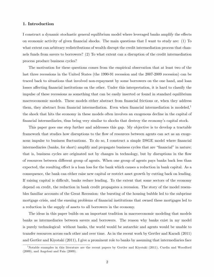
1. Introduction

I construct a dynamic stochastic general equilibrium model where leveraged banks amplify the e¤ects

on economic activity of given �nancial shocks. The main questions that I want to study are: (1) To

what extent can arbitrary redistributions of wealth disrupt the credit intermediation process that chan-

nels funds from savers to borrowers? (2) To what extent can a disruption of the credit intermediation

process produce business cycles?

The motivation for these questions comes from the empirical observation that at least two of the

last three recessions in the United States (the 1990-91 recession and the 2007-2009 recession) can be

traced back to situations that involved non-repayment by some borrowers on the one hand, and loan

losses a¤ecting �nancial institutions on the other. Under this interpretation, it is hard to classify the

impulse of these recessions as something that can be easily inserted or found in standard equilibrium

macreoconomic models. These models either abstract from �nancial frictions or, when they address

them, they abstract from �nancial intermediation. Even when �nancial intermediation is modeled,1

the shock that hits the economy in these models often involves an exogenous decline in the capital of

�nancial intermediaries, thus being very similar to shocks that destroy the economy�s capital stock.

This paper goes one step further and addresses this gap. My objective is to develop a tractable

framework that studies how disruptions to the �ow of resources between agents can act as an exoge-

nous impulse to business �uctuations. To do so, I construct a simple DSGE model where �nancial

intermediaries (banks, for short) amplify and propagate business cycles that are ��nancial�in nature;

that is, business cycles are originated not by changes in technology, but by disruptions in the �ow

of resources between di¤erent group of agents. When one group of agents pays banks back less than

expected, the resulting e¤ect is a loan loss for the bank which causes a reduction in bank capital. As a

consequence, the bank can either raise new capital or restrict asset growth by cutting back on lending.

If raising capital is di¢ cult, banks reduce lending. To the extent that some sectors of the economy

depend on credit, the reduction in bank credit propagates a recession. The story of the model resem-

bles familiar accounts of the Great Recession: the bursting of the housing bubble led to the subprime

mortgage crisis, and the ensuing problems of �nancial institutions that owned these mortgages led to

a reduction in the supply of assets to all borrowers in the economy.

The ideas in this paper builds on an important tradition in macroeconomic modeling that models

banks as intermediaries between savers and borrowers. The reason why banks exist in my model

is purely technological: without banks, the world would be autarchic and agents would be unable to

transfer resources across each other and over time. As in the recent work by Gertler and Karadi (2011)

and Gertler and Kiyotaki (2011), I give a prominent role to banks by assuming that intermediaries face

1Notable examples in this literature are the recent papers by Gertler and Kiyotaki (2011), Curdia and Woodford(2009), and Angeloni and Faia (2009).

2

a balance sheet constraint when obtaining deposits. In these papers however, the shock that causes a

�nancial business cycle is a shock to the quality of bank capital that triggers a decline in asset values

and the ensuing recession, and is calibrated in order to produce a downturn of similar magnitude to

the one observed in the data. Instead, I calibrate the size of the shock by using information on losses

su¤ered by �nancial institutions during the Great Recession, and break the propagation down into

various pieces, in order to see under which conditions losses of the extent seen in the data can produce

a large recession. I then show that a persistent repayment shock that causes bank equity to fall by

about 5 percent of GDP over a four-year period, total GDP losses can be of similar magnitude to what

observed in the data.

2. The Model

I consider a discrete-time, perfect foresight economy. The economy features two household types;

entrepreneurs; bankers, and a �nal goods �rm. A summary of the model setup in in Figure 1.2

Households work, consume and buy houses, and deposit resources into (or borrow from) a bank

through one-period loans: in order to model heterogeneity and household credit within households in

a tractable fashion, households are divided into patient savers and impatient borrowers. To �x ideas,

I interpret the impatient borrowers as subprime people (subprimers from now on): as argued in the

introduction, the idea that I want to explore is that the original shock that hits the system starts from

the decision of these agents not to repay their loans. As a whole, the household sector is a net supplier

of savings to the rest of the economy.

Entrepreneurs accumulate physical capital (which they rent to a representative �rm) and borrow

from banks, subject to a collateral constraint. Not all owners of capital are credit constrained though:

in order to control the extent and severity of �nancial frictions on the production side, I allow patient

households to accumulate part of the economywide capital stock. This way, to the extent that the size

of impatient households and entrepreneurs becomes arbitrarily small, banks become arbitrarily small

too (since there are no fund to intermediate between savers and borrowers), and the model boils down

to the canonical RBC/growth model.

2Except for the introduction of the banking sector, the model structure closely follows a �exible price version ofthe model in Iacoviello (2005). Except for the introduction of the banking sector, the main di¤erence is that I allowhousehold savers to also accumulate productive capital, so that I can nest the RBC model as a special case. I alsodistinguish between entrepreneurs (who produce capital) and good producers (who rent capital from entrepreneurs andlabor from households), but this distinction is only a matter of expositional convenience, and bears no implications forthe results.

3

Figure 1: Summary of the Model Structure

Bankers intermediate funds between patient savers on the one hand, and entrepreneurs and sub-

primers on the other. The nature of the banking activity implies that bankers are borrowers when it

comes to their relationship with households, and are lenders when it comes to their relationship with

the credit-dependent sectors (entrepreneurs and subprimers) of the economy. I design preferences in

a way that two frictions coexist and interact in the model�s equilbrium: �rst, bankers�are credit con-

strained in how much they can borrow from the patient savers; second, entrepreneurs and subprimers

are credit constrained in how much they can borrow from bankers. My interest is in understanding

how these two frictions interact with and reinforce each other.

Finally, the representative �rm converts entrepreneurial capital and household labor into the �nal

good using a constant-returns-to-scale technology.

Patient Households. There is a continuum of measure 1 of savers (indexed by H). I measure their

economic size by controlling their wage share in production (either patient households or impatient

households work) and their capital share in production (either patient households or entrepreneurs

accumulate physical capital).

4

They choose consumption C, housing H (which has zero depreciation), physical capital K (which

depreciates at rate � and incurs a standard convex adjustment cost) and time spent working N to

solve the following intertemporal problem:

maxE0

1Xt=0

�tH (logCH;t + j logHH;t + � log (1�NH;t))

where �H is the discount factor, subject to the following �ow-of-funds constraint:

CH;t+KH;t+�KH;t+Dt+qt (HH;t �HH;t�1) = (RM;t + 1� �)KH;t�1+RH;t�1Dt�1+WH;tNH;t (2.1)

where D denotes bank deposits (earning a gross return RH), q is the price of housing in units of

consumption/�nal good, WH is the wage rate, and RK is the rental rate for capital. Housing does not

depreciate. The capital adjustment cost function takes the form �KH;t = �KH (KH;t �KH;t�1)2. Theoptimality conditions yield standard �rst-order conditions for consumption/deposits, housing demand,

capital supply, and labor supply.

1

CH;t= �HEt

�1

CH;t+1RH;t

�(2.2)

qtCH;t

=j

HH;t+ �HEt

�qt+1CH;t+1

�(2.3)

1

CH;t

�1 +

@�KH;t@KH;t

�= �HEt

�1

CH;t+1

�RM;t+1 + 1� � +

@�KH;t+1@KH;t

��(2.4)

WH;t

CH;t=

�

1�NH;t. (2.5)

Subprimers (Impatient Households, Borrowers). Subprimers (indexed by S) do not save and

borrow up to a fraction of the value of their house. They solve:

maxE0

1Xt=0

�tS (logCS;t + j logHS;t + � log (1�NS;t))

subject to the �ow-of-funds constraint and the borrowing constraint:

CS;t + qt (HS;t �HS;t�1) +RS;t�1LS;t�1 � "t = LS;t +WS;tNS;t (2.6)

LS;t � Et�1

RS;tmSqt+1HS;t

�. (2.7)

The borrowing constraint limits borrowing to the present discounted value of their housing holdings.

Below, I will show that the constraint binds in a neighborhood of the non-stochastic steady state if �S

is lower than a weighted average of the discount factors of patient households and bankers. The term

LS denotes (one-period) loans made to subprimers, paying a gross interest rate RS : Finally the term

5

"t in the budget constraint denotes an exogenous repayment shock: I assume that subprimers can pay

back less (more) than agreed on their contractual obligations if " is greater (smaller) than zero; from

their point of view, this shock represents �all else equal �a positive shock to wealth, since it allows

them to spend more than previously anticipated.

The optimality conditions for debt, housing demand and labor supply will be:

1� �S;tCS;t

= �SEt

�RS;tCS;t+1

�(2.8)

Et

�1

CS;t

�qt � �S;tmS

qt+1RS;t

��=

j

HS;t+ �SEt

�qt+1CS;t+1

�(2.9)

WS;t

CH;t=

�S1�NS;t

. (2.10)

Above, �S;t denotes the Lagrange multiplier on the borrowing constraint. A positive value of the

multiplier works to reduce the current user cost of housing, denoted by qt � �S;tmSqt+1RS;t

; and tilts

preferences towards housing goods (relative to consumption goods), as emphasized for instance in

Monacelli (2009).

Note that one could endogenize the repayment shock in other ways: for instance, one could assume

that if house prices fall below some value, borrowers could �nd it optimal to default rather than roll

their debt over: defaulting would be equivalent to choosing a value for RS;tLS;t�1 lower than previously

agreed, which would generate the same e¤ect as a positive shock to "t.

Entrepreneurs. A continuum of unit measure entrepreneurs solve the following problem:

maxE0

1Xt=0

�tE logCE;t

subject to:

CE;t +KE;t + �KE;t + qt (HE;t �HE;t�1) +RE;tLE;t�1 = LE;t + (RK;t + 1� �)KE;t�1 +RV;tHE;t�1(2.11)

LE;t � mHEt

�qt+1RE;t

HE;t

�+mEKE;t (2.12)

Here, LE are loans that banks extend to entrepreneurs (yielding a gross return RE), KE is capital that

entrepreneurs rent to a goods producing �rm at the rate RK , and � is the capital depreciation rate.

Entrepreneurs also accumulate housing (commercial real estate) which they rent to the �nal good �rm

at the rate RV . Entrepreneurs cannot borrow more than a fraction mE of their hard assets KE , and a

fractionmH of their real estate capital qHE . As for the case of impatient borrowers, this constraint will

be binding near the non-stochastic steady state, provided that entrepreneurs are impatient enough.

6

The term �KE;t denotes convex capital adjustment costs, denoted by �KE;t = �KE (KE;t �KE;t�1)2.The entrepreneur�s �rst-order conditions can be written as:

1� �E;tCE;t

= �EEt

�RE;t+1CE;t+1

�(2.13)

1

CE;t

�1� �E;tmK +

@�KE;t@KE;t

�= �EEt

�1

CE;t+1

�1� � +RK;t+1 +

@�KE;t+1@KE;t

��(2.14)

Et

�1

CE;t

�qt � �E;tmH

qt+1RE;t

��= �EEt

�qt+1

1 +RV;t+1CE;t+1

�(2.15)

Bankers. A continuum of unit measure bankers solve the following problem:

max1Xt=0

�tB logCB;t

subject to:

CB;t +RH;t�1Dt�1 + LE;t + LS;t = Dt +RE;tLE;t�1 +RS;t�1LS;t�1 � "t (2.16)

where the right-hand side measures the sources of funds for the bank (net of adjustment costs and

loan losses): D are household deposits, and RELE and RSLS are repayments from entrepreneurs and

subprimers on previous period loans. The funds can be used by the bank to pay back depositors and

to extend new loans, or can be used for banker�s consumption. Note that this formulation is analogous

to a formulation where bankers maximize a convex function of dividends (discounted at rate �B), once

CB is reinterpreted as the residual income of the banker after depositors have been repaid and loans

have been issued.

In a frictionless model, one implicitly assumes that deposits can be costlessly converted into loans.

Here instead I assume that the bank is constrained in its ability to issue liabilities by the amount of

equity capital (assets less liabilities) in its portfolio. This constraint can be motivated by regulatory

concerns or by standard moral hazard problems: for instance, typical regulatory requirements (such

as those agreed by the Basel Committee on Banking Supervision) posit that banks hold a capital to

assets ratio greater than or equal to some predetermined ratio. Letting KBt = LE;t + LS;t � "t �Dtde�ne bank capital at the end of the period (after loan losses have been realized), a capital requirement

constraint can be reinterpreted as a standard borrowing constraint, such as:

Dt � ELE;t + S (LS;t � "t) . (2.17)

Above, the left-hand side denotes banks liabilities Dt; while the right-hand side denotes which fraction

7

of each of the banks�assets can be used as collateral.3

Denote with �B;t the multiplier on the bank�s borrowing constraint (later, I will show the conditions

that ensure that the constraint is binding). Let mB;t = �BEt

�CB;t+1CB;t

�denote the banker�s stochastic

discount factor, The bank�s optimality conditions for deposits, loans to entrepreneurs and loans to

subprimers are respectively:

1� �B;t = Et (mB;tRH;t) (2.18)

1� E�B;t = Et (mB;tRE;t+1) (2.19)

1� S�B;t = Et (mB;tRS;t) . (2.20)

The interpretation of these �rst-order condition is straightforward. It also illustrates why the

di¤erent classes of assets pay di¤erent returns in equilibrium. Consider the ways a bank can increase

its consumption by one extra unit today.

1. The banker can borrow from household, increasing D by one unit today: in doing so, the bank

reduces its equity by one unit too, thus tightening its borrowing constraint one�for�one and

reducing the utility value of an extra deposit by �B. Next period, when the bank pays the

deposit back, the cost is given by the stochastic discount factor times the interest rate RH .

2. The banker can consume more today by decreasing loans to, say, entrepreneurs, by one unit. By

lending less to the entrepreneurs, the bank tightens its borrowing constraint, (since it reduces

its equity, loans minus deposits), thus incurring a utility cost equal to E�B;t; hence the cost is

larger the larger E is: intuitively, the more loans are useful as collateral for the bank activity,

the larger the utility cost of not making loans.

For the bank to be indi¤erent between collecting deposits (borrowing) and making loans (saving),

the returns on all assets must be equalized. Given that RH is determined from the household problem,

the banker will be borrowing constrained, and �B will be positive, so long as mB;t is su¢ ciently lower

than the inverse of RH . In turn, if �B is positive, the returns on loans RE and RS will be lower, the

lower E and S are. Intuitively, the larger is, the higher is the liquidity value of loans for bank

in relaxing its borrowing constraint, and the smaller the compensation required for the bank to be

indi¤erent between lending and borrowing. Moreover, loans will pay a return that is (near the steady

state) higher than the cost of deposits, since, so long as is lower than one, they are intrinsically less

liquid than the deposits.

In the quantitative implementation of the model, I allow for a more �exible form of the bank

capital constraint that allows the bank some �exibility in satisfying its capital requirement. To do so,3 In the simple case where E = S = < 1, the fraction E

L= 1 � can be interpreted as the bank�s capital-asset

ratio, while LE= 1

1� denotes the bank�s leverage ratio (the ratio of bank�s liabilties to its equity).

8

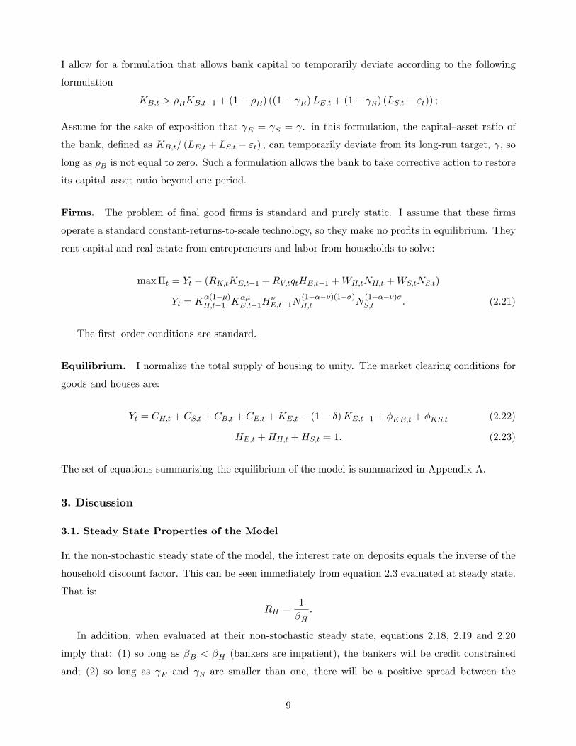
I allow for a formulation that allows bank capital to temporarily deviate according to the following

formulation

KB;t > �BKB;t�1 + (1� �B) ((1� E)LE;t + (1� S) (LS;t � "t)) ;

Assume for the sake of exposition that E = S = . in this formulation, the capital�asset ratio of

the bank, de�ned as KB;t= (LE;t + LS;t � "t) ; can temporarily deviate from its long-run target, ; so

long as �B is not equal to zero. Such a formulation allows the bank to take corrective action to restore

its capital�asset ratio beyond one period.

Firms. The problem of �nal good �rms is standard and purely static. I assume that these �rms

operate a standard constant-returns-to-scale technology, so they make no pro�ts in equilibrium. They

rent capital and real estate from entrepreneurs and labor from households to solve:

max�t = Yt � (RK;tKE;t�1 +RV;tqtHE;t�1 +WH;tNH;t +WS;tNS;t)

Yt = K�(1��)H;t�1 K

��E;t�1H

�E;t�1N

(1����)(1��)H;t N

(1����)�S;t . (2.21)

The �rst�order conditions are standard.

Equilibrium. I normalize the total supply of housing to unity. The market clearing conditions for

goods and houses are:

Yt = CH;t + CS;t + CB;t + CE;t +KE;t � (1� �)KE;t�1 + �KE;t + �KS;t (2.22)

HE;t +HH;t +HS;t = 1. (2.23)

The set of equations summarizing the equilibrium of the model is summarized in Appendix A.

3. Discussion

3.1. Steady State Properties of the Model

In the non-stochastic steady state of the model, the interest rate on deposits equals the inverse of the

household discount factor. This can be seen immediately from equation 2.3 evaluated at steady state.

That is:

RH =1

�H.

In addition, when evaluated at their non-stochastic steady state, equations 2.18, 2.19 and 2.20

imply that: (1) so long as �B < �H (bankers are impatient), the bankers will be credit constrained

and; (2) so long as E and S are smaller than one, there will be a positive spread between the

9

return on loans and the cost of deposits. The spread will be larger the tighter the capital requirement

constraint for the bank. Formally:

�B = 1� �BRH = 1��B�H

> 0 (3.1)

RE = E1

�H+ (1� E)

1

�B> RH (3.2)

RS = S1

�H+ (1� S)

1

�B> RH . (3.3)

I turn now to entrepreneur and subprimers. Given the interest rates on loans RE and RS , a

necessary condition for entrepreneur and subprimers to be constrained is that their discount factor is

lower than the inverse of the return on loans above. When this condition is satis�ed (that is �ERE < 1

and �SRS < 1); entrepreneurs and subprimers will be constrained in a neighborhood of the steady

state. Alternatively, this condition requires that entrepreneurs�and subprimers�discount factors are

lower than a weighted average (geometric mean) of the discount factors of households and banks.

�E <1

E1�H+ (1� E) 1

�B

�S <1

S1�H+ (1� S) 1

�S

It is also easy to show that both the bankers� credit constraint and the entrepreneurs� credit

constraint create a positive wedge between the steady state output in absence of �nancial frictions

and the output when �nancial frictions are present. The credit constraint on banks limits the amount of

deposits (savings) that banks can transform into loans. Likewise, the credit constraint on entrepreneurs

limits the amount of loans that can become physical capital. Both forces work to reduce the amount

of savings that can be transformed into capital, thus lowering steady state output. The same forces

are also at work for shocks that move the economy away from the steady state, to the extent that

these shocks tighten or loosen the severity of the borrowing constraints.

3.2. Dynamic Properties of the Model

To gain some intution into the workings of the model, it is useful to consider how time-variation in the

tightness of the bankers�borrowing constraint can a¤ect equilibrium dynamics. To do so, it is useful

to focus both on the price and the quantity side of the story.

I begin with the price side. For the sake of argument, consider a perfect foresight version of the

model, so that variables are equal to their expected values. In this case, in the limiting case of no

adjustment costs, the expression for the spread between the return on loans and the cost of deposits

10

can be written as:

Et (RE:t+1)�RH;t =�B;tmB;t

(1� E) .

According to this expression, the spread between the return on entrepreneurial loans and the cost of

deposits gets larger whenever the banker�s borrowing constraint gets tigher (an analogous expression

holds for the spread between RS;t and RH;t). Intuitively, when the capital constraint gets tighter

(for instance because bank net worth is lower), the bank requires a larger compensation on its loans

in order to be indi¤erent between making loans and issuing deposits. This occurs because loans are

intrinsically more illiquid than deposits: when the constraint is binding, a reduction in deposits of 1

dollar requires cutting back on loans by 1 Edollars. All else equal, a rise in the spread will act as a

drag on economic activity during periods of lower bank net worth.

Now I move to the quantity side: whenever a shock causes a reduction in bank capital, the logic of

the balance sheet requires for the bank to contract its asset side by a multiple of its capital, in order

for the bank to restore its leverage ratio. The bank could avoid this by raising new capital (reducing

bankers�consumption), but the bankers�impatience motive and the weak economy make this route

impractical or, at best, insu¢ cient. As a consequence, the bank reduces its lending. If a substantial

part of the economy depends on bank credit to run its activities, the contraction in bank credit causes

in turn a decrease in economic activity.

The obvious test of the model is: can bank losses of the magnitude occurred in the last couple of

years justify a sharp, large and protracted drop in economic activity? Before I assess the quantitative

signi�cance of this mechanism, I need to calibrate the model.

3.3. The Model without Banks

As a reference point, it is useful to illustrate the key di¤erences between the model above and a model

without banks, or, alternatively, a model where banks are a pure veil and frictionlessy intermediate

funds between borrowers and savers. In such a model, all savings are converted into loans, so that

equation 2.17 is replaced by the identity

Dt = LE;t + LS;t. (3.4)

Moreover, bankers disappear from the model, so that CB;t = 0 and �B;t = 0. In addition, the

relevant discount factor to price loans is the patient household�s stochastic discount factor mH;t =

�HEt

�CH;t+1CH;t

�.

11

4. Calibration

I begin with standard preference and technology parameters. The patient household discount factor is

set at �H = 0:9925: The entrepreneurial discount factor is 0:96: The subprimers discount factors is set

at 0:96. I set the capital share � = 0:35 and its depreciation rate � = 0:035: These parameters imply a

steady state 3 percent return annualized on deposits, a capital-output ratio of 1:85 (annualized), and

an investment to output ratio of 26 percent. I assume that the share of patient households�capital

in production is � = 0:5, which results in 53 percent of the capital stock accruing to agents that are

not credit constrained (and 47 accruing to the constrained entrepreneurs). As for real estate, I set

the share of commercial real estate in production � at 0:05, and the weight on housing in utility at

j = 0:08 : these numbers yield a ratio of real estate wealth to output of 2:1 (annualized), of which 0:8

is commercial real estate, 1:3 is residential real estate.

The weights on leisure in the utility function of both households, �H and �S , are set at 2: This

numbers implies that individuals work about one third of their time endowment, and that the Frisch

labor supply elasticity is around 2.

For the parameters controlling leverage, I choose mE = 0:9, mS = 0:9, mK = 0:9, S = 0:9

and E = 0:9: I also set the income share of impatient households/subprimers to � = 0:30. These

parameters imply that the leverage ratio of the production side of the economy is about 0:55; consistent

with data from the Flow of Funds for leverage of the business sector. The leverage ratio of the household

sector is about 0:14: this value is lower than the data counterpart (which, depending on the measure, is

about three times bigger), but I choose to be conservative on this value because many mortgages are in

the data held by households who are not necessarily credit constrained. Finally, the leverage parameter

for the bank is consistent with aggregate data on bank balance sheets that show capital�asset ratios

for banks close to 0:1.

I set the discount factors for the bankers at �B = 0:965. Together with the bank leverage para-

meters, these values imply a spread of about 1 percent (on an annualized basis) between lending and

deposit rates.

The capital adjustment cost parameters �KE and �KH are set at 2; which is consistent with the

estimates of capital adjustment costs that are found in the literature. The parameter determining the

inertia of the equity requirement for the bank, �B; is set equal at 0:5: this parameter has little e¤ect

on the model dynamics, with higher values of this parameter slowing down the response of spreads to

�nancial shocks.

Finally, I assume that the process for the repayment shock follows an AR(1) process with autocor-

relation coe¢ cient of 0:9. When the shock �rst hits, most of its e¤ects work through the expectations

of further losses in the future.4

4 In simulations not reported here, I have veri�ed that the e¤ects of the shock are qualitatively similar if one models

12

5. Properties of the Model

5.1. The Baseline Financial Shock

The thought experiment that I consider is the following. What are the consequences of a �nancial

shock in this model? Of course, the experiment begs the question: what is a �nancial shock?

One possibility is that a �nancial shock is something that a¤ects the ability of a bank to transform

savings into loans. However, this shock is very similar to an investment-biased technology shock,

and almost assumes the conclusions: moreover, we already know that this shock (see the discussion

in Justiniano, Primiceri and Tambalotti, 2010) has a somewhat hard time (in absence of bells and

whistles) in generating the joint comovement of consumption, investment and hours that is the essence

of business cycles. Another possibility is that the �nancial shock captures an exogenous disturbance to

the wedge between the cost of funds paid by borrowers and the return on funds received by lenders (see

Hall, 2010, for such an interpretation): however, it is hard to give a general equilibrium interpretation

of this shock, and one would like to believe that changes in spreads are the e¤ect, not the cause, of

�nancial shocks.

For my purposes, I want to give to the �nancial shock a di¤erent interpretation that starts by

directly feeding into the model the losses that the shock causes. I want to think of this shock as purely

redistributive in nature: for some unmodeled reason, the shock starts with one group of agents paying

back less than initially agreed on their obligations. I assume these agents are the subprimers. Hence

the shock I consider has a dual nature: from the lender�s (bank) point of view, it is equivalent to an

exogenous destruction of the lender�s assets (a negative wealth shock); however, from the borrowers�

point of view, it is equivalent to a positive shock to wealth. Now, it is obvious that the �nancial shock

was not exogenous: one could argue that the real trigger of the crisis was the decline in housing prices

that led to defaults that led to non�repayments, but �rst�hand evidence suggests that the big fallout

on economic activity from the decline in housing prices did not occur until banks were forced by loan

losses to take dramatic measures to reduce the size of their balance sheets.

The next question to consider is: how big is the shock? I can use available data on quantities to

get a sense of its size. Any unexpected non-repayment from the borrower causes a loss of the same

amount for a lender. I use the estimates of bank losses following the �nancial crisis to gauge how big

the shock is. In particular, I use estimated loan writedowns for the years between 2007 and 2010,

as calculated by the IMF�s Global Financial Stability Report (in April 2009).5 The Global Financial

Stability Report estimates loan losses for U.S. banks over the 2007-2010 period of 1.07 trillion dollars,

that is, about 9 percent of private GDP; focusing on the 2007�2008 period, the losses are slightly

the �nancial shock as a sequence of unexpected repayment shocks.5See http://www.imf.org/external/pubs/ft/gfsr/2009/01/pdf/text.pdf, Table 1.3.

13

smaller, about 6 percent of private GDP.6 Using this information, I calibrate the �nancial shock as

a persistent repayment shock that results, after a two-year period, in cumulative losses of around 6

percent of private GDP. My maintained assumption is that banks do not react to the shock by charging

higher interest rates (to make up for the losses or for the higher risk).

How does the �nancial shock work? Figure 2 plots the dynamic simulations for my model economy.7

The negative repayment shock impairs the bank�s balance sheet, by reducing the value of the

banks�assets (total loans minus loan losses) relative to the liabilities (in the model, these are household

deposits): at that point, in absence of any further adjustment to either loans or deposits, the bank

would have a capital asset ratio that is below target. The banker can restore its capital-asset ratio

either deleveraging (reducing its deposits from households), or reducing consumption in order to

restore its equity cushion. Reducing consumption only is too costly for the banker: as a consequence,

in the baseline scenario, the bank cuts bank on its loans too, and begins a vicious, dynamic circle of

simultaneous reduction both in loans and deposits, thus propagating the credit crunch. In particular,

the decline in all types of loans to the credit-dependent sectors of the economy (entrepreneurs and

subprimers) acts a drag on both consumption and investment. Note that aggregate consumption

initially moves little re�ecting the increased consumption of the borrowers who pay back less, and the

reduced consumption of bankers and entrepreneurs. And that spreads rise re�ecting the high utility

cost of making a loan for the bank in a period in which banker�s consumption and equity are low. And

note that in absence of deleveraging (top right panel) the bank would �nd itself nearly insolvent (its

capital asset ratio would go to almost zero): the deleveraging, in turn, forces a reduction in loans.

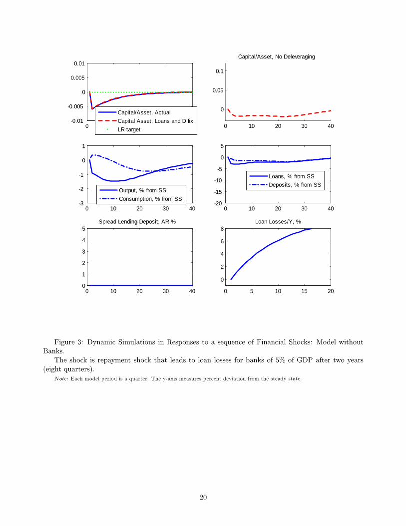
By contrary, in a model where banks are not forced to restore their capital�asset ratio because they

are just a veil, the losses are much smaller. The e¤ects are shown in Figure 3. The �nancial shock works

like a pure redistribution shock that transfers wealth from agents from agents with a low marginal

propensity to consume (the households who deposit their savings into the bank) to agents with a high

marginal propensity to consume (the subprimers). The main e¤ect of this shock works through labor

supply. Subprimers work less (because their wealth is higher), savers work more (because their wealth

is lower). Because subprimers have higher wealth, they can increase their borrowing and housing

demand, thus crowding out some of the household savings away from the entrepreneurial sector. In

the aggregate, the e¤ects on economic activity are negative but small, only one third as large as those

in the model with credit�constrained banks.6These numbers are roughly in line with estimates of loan losses published by the Federal Financial Institutions

Examination Council based on Call Reports data. Between 2007 and 2010, net loan losses as a fraction of total loansfor all U.S. Banks rose from about 0.4 to about 3 percent; and loan loss reserves rose from about 1 percent to about 4percent.

7The economy is assumed to be in steady state in period 1, and the shock hits in period 2.

14

5.2. Breaking Down the Financial Shock

The e¤ects through which the �nancial shock operates are broken down in Figure 4 (for output) and

Figure 5 (for consumption, investment and other model variables). Figure 4 plots the total loss in

output (as a percentage of its initial level) in various versions of the model where the various frictions

are shut o¤. Figure 5 o¤ers a more comprehensive picture plotting deviations from baseline for the

various model variables.

To illustrate the strengths of the various channels in shaping output dynamics in response to a

�nancial shock, I start from the simplest model where labor supply is completely inelastic (so that

�H and �S both approach zero), the banking channel is shut down, and collateral e¤ects on �rms

are absent, so that constrained entrepreneurs are not allowed to borrow (mH and mK are zero) and

their shares in production (� and �) approach zero. The only e¤ect of the �nancial shock is that of

transferring wealth away from the savers towards the borrowers. On the one hand, borrowers consume

more. On the other hand, household savers consume less, but also save less in order to smooth their

consumption, so that the decline in their consumption does not fully o¤set the rise in borrowers�

consumption, and aggregate consumption rises. However, the decline in saving leads to a decline in

investment that more than o¤sets the rise in consumption, so that aggregate output falls, although

the total e¤ects are very small. As a fraction of steady�state annual GDP, the total output losses are

only 1.5 percent after 10 years.

Consider next what happens when labor supply is assumed to be elastic, as in the benchmark case,

but banking and collateral frictions are still shut o¤. There is now an additional e¤ect that works

through the di¤erential e¤ects on labor supply induced by the �nancial shock. On the one hand,

borrowers consume more, and, as can be seen from their labor supply equation, they also work less.

However, because savers�consumption does not fall to fully o¤set the rise in borrowers�consumption,

their increase in hours does not fully o¤set the decline in hours of the borrowers. As hours fall in the

aggregate, capital �which is complementary to labor in the production function �also falls over time

(over and above the e¤ect caused by the decline in savers�consumption), and the total output loss

is now larger, at around 5 percent. Note that here the decline in output comes both from a decline

in labor demand (as capital falls because of the reduced savings, the marginal product of labor falls)

and from a decline in labor supply. The story here echoes Mulligan (2010)�s idea that labor market

distortions were at the core of the recession: for instance, Mulligan (2010) argues that renegotiations

of business debts, student loans, and tax debts presented debtors with disincentives to work. In the

general equilibrium model presented here, the disincentives to work for the debtors are not fully o¤set

by the larger incentives to work for the creditors, since debtors�consumption is not determined by their

consumption Euler equation (they are facing a borrowing constraints), while creditors�consumption

is. Hence the net e¤ect of a �nancial shock is an aggregate decline in labor supply.

15

The above e¤ects are further reinforced when the collateral channel is turned on. The decline in

output leads to a decline in asset prices and in the collateral capacity of credit�constrained �rms,

which exacerbates the decline in output and investment relative to a model in which all productive

capital is held by unconstrained households. The overall output loss is about 9 percent after 10 years.8

Finally, the largest negative e¤ects on economic activity from the �nancial shock occur when both

the banking channel and the collateral channel are at work, thus restoring the baseline model. By

putting direct pressure on the bank�s balance sheet, the �nancial shock further strengthens the drop

in output, and the total output loss after 10 years is about 18 percent (it is around 9 percent after

two years).

6. Concluding Remarks

In this paper I have presented a simple model where losses incurred by banks can produced sizeable,

pronounced and long-lasting e¤ects on business activity. The key ingredients of the model are regu-

latory constraints on the leverage of the banks and a business sector that is bank�dependent for its

operations.

A simple back�of�the�envelope calculation illustrates how big these e¤ects are relative to the data.

According to the model, a realistically calibrated �nancial shock can induce a cumulated GDP loss

of nearly 8 percent after 3 years, which would correspond to the 2008-2010 period for which we have

available data to compare with the model. The data counterpart, depending on the method that one

uses to detrend GDP, ranges from 11 percent (for HP-�lter) to 14 percent (using the CBO estimates of

potential output) 18 percent (detrending GDP using a quadratic trend).9 Hence the model can account

for values between 40 and 75 percent of the entire decline in output during the Great Recession. A

somewhat larger labor supply elasticity, higher intensity of �nancial frictions, and smaller capital

adjustment costs could explain all of the decline in output in the data.

8When the collateral channel is present, the endogenous reduction in the capital stock reduces labor demand. In thissetup, the reduction in hours comes both from reduction in labor supply and from the reduction in labor demand.

9To measure the cumulated output loss in the data, I detrend real GDP using one of the three methods described inthe text. I then normalize the resulting series �regardless of what the detrending method says �so that GDP is rightaround trend in 2007Q4. I then compute the cumulated, annualized sum of all deviations from trend of the normalizedseries.

16

References

[1] Angeloni, Ignazio, and Ester Faia (2009). �A Tale of Two Policies: Prudential Regulation andMonetary Policy with Fragile Banks,�Kiel Working Papers 1569, Kiel Institute for the WorldEconomy

[2] Bernanke, Ben S., and Gertler, Mark (1995). �Inside the Black Box: The Credit Channel ofMonetary Policy Transmission.�Journal of Economic Perspectives, Fall 1995, 9 (4), pp. 27-48.

[3] Blanchard, Olivier (2008). �The Crisis: Basic Mechanisms, and Appropriate Policies.�, workingpaper, MIT and IMF.

[4] Curdia, Vasco, and Michael Woodford (2009), �Conventional and Unconventional Monetary Pol-icy�, working paper, FRBNY and Columbia.

[5] Gertler, Mark, and Peter Karadi (2011), �A model of unconventional monetary policy,�Journalof Monetary Economics

[6] Gertler, Mark, and Nobuhiro Kiyotaki (2011), �Financial Intermediation and Credit Policy inBusiness Cycle Analysis�, working paper, NYU and Princeton.

[7] Greenlaw, D., Hatzius, J., Kashyap, A. and Shin, H. S. (2008). Leveraged losses: lessons from themortgage market meltdown , Report of the US Monetary Monetary Form, No. 2.

[8] Hall, Robert (2009). �The High Sensitivity of Economic Activity to Financial Frictions,�workingpaper, Stanford University.

[9] IMF (2009). �Global Financial Stability Report. Responding to the Financial Crisis and MeasuringSystemic Risk�, April.

[10] Iacoviello, Matteo (2005). �House Prices, Borrowing Constraints and Monetary Policy in theBusiness Cycle.�American Economic Review, June, 95 (3), pp. 739-764.

[11] Justiniano, Alejandro, Giorgio E. Primiceri, and Andrea Tambalotti (2010), �Investment shocksand business cycles�, Journal of Monetary Economics, 57, 2, 132-145.

[12] Monacelli, Tommaso (2009). �New Keynesian Models, Durable Goods and Borrowing Con-straints,�Journal of Monetary Economics

[13] Mulligan, Casey (2010). �Aggregate Implications of Labor Market Distortions: The Recession of2008-9 and Beyond,�NBER Working Paper No. 15681.

17

Appendix A. The Complete Model Equations.

I summarize here the equations describing the equilibrium of the model.

CH;t +KH;t +Dt + qt�HH;t = (RM;t + 1� �)KH;t�1 +RH;t�1Dt�1 +WH;tNH;t (6.1)

1=CH;t = �HEt (RH;t=CH;t+1) (6.2)

WH;t (1�NH;t) = �HCH;t (6.3)

1=CH;t = �HEt ((RM;t+1 + 1� �) =CH;t+1) (6.4)

CS;t + qt�HS;t +RS;t�1LS;t�1 � "t = LS;t +WS;tNS;t (6.5)

LS;t = mSEt (qt+1HS;t=RS;t) (6.6)

(1� �S;t) =CS;t = �SEt (RS;t=CS;t+1) (6.7)

WS;t (1�NS;t) = �SCS;t (6.8)

CB;t +RH;t�1Dt�1 + LE;t + LS;t = Dt +RE;tLE;t�1 +RS;t�1LS;t�1 � "t (6.9)

Dt = ELE;t + SLS;t (6.10)

(1� �B;t) =CB;t = �BEt (RH;t=CB;t+1) (6.11)

(1� E�B;t) =CB;t = �BEt (RE;t+1=CB;t+1) (6.12)

(1� S�B;t) =CB;t = �BEt (RS;t=CB;t+1) (6.13)

CE;t +KE;t + qt�HE;t +RE;�1LE;�1 = RV;tqtHE;t�1 + (RK;t + 1� �)KE;t�1 + LE;t (6.14)

LE;t = mHEt

�qt+1RE;t

HE;t

�+mKKE;t (6.15)

(1� �E;t) =CE;t = �EEt (RE;t=CE;t+1) (6.16)

(1� �E;tmK) =CE;t = �EEt ((1� � +RK;t+1) =CE;t+1) (6.17)

Yt = K�(1��)H;t�1 K

��E;t�1H

�E;t�1N

(1����)(1��)H;t N

(1����)�S;t (6.18)

��Yt = RK;tKE;t�1 (6.19)

� (1� �)Yt = RM;tKH;t�1 (6.20)

�Yt = RV;tqtHE;t�1 (6.21)

(1� �� �) (1� �)Yt =WH;tNH;t (6.22)

(1� �� �)�Yt =WS;tNS;t (6.23)

Et ((qt � �E;tmHqt+1=RE;t) =CE;t) = �EEt (qt+1 (1 +RV;t+1) =CE;t+1) (6.24)

qt=CH;t = j=HH;t + �HEt (qt+1=CH;t+1) (6.25)

Et ((qt � �S;tmSqt+1=RS;t) =CS;t) = j=HS;t + �SEt (qt+1=CS;t+1) (6.26)

HH;t +HS;t +HE;t = 1 (6.27)

18

0 10 20 30 40

0.095

0.1

0.105

Capital/Asset, ActualCapital Asset, Loans and D fixLR target 0 10 20 30 40

0

0.05

0.1

Capital/Asset, No Deleveraging

0 10 20 30 40­3

­2

­1

0

1 Output, % from SSConsumption, % from SS

0 10 20 30 40­20

­15

­10

­5

0

5

Loans, % from SSDeposits, % from SS

0 10 20 30 400

1

2

3

4

5Spread Lending­Deposit, AR %

0 5 10 15 20

0

2

4

6

8Loan Losses/Y, %

Figure 2: Dynamic Simulations in Responses to a sequence of Financial Shocks: baseline bankingmodel.

The shock is repayment shock that leads to loan losses for banks of 5% of GDP after two years(eight quarters).

Note: Each model period is a quarter. The y-axis measures percent deviation from the steady state.

19

0 10 20 30 40­0.01

­0.005

0

0.005

0.01

Capital/Asset, ActualCapital Asset, Loans and D fixLR target 0 10 20 30 40

0

0.05

0.1

Capital/Asset, No Deleveraging

0 10 20 30 40­3

­2

­1

0

1

Output, % from SSConsumption, % from SS

0 10 20 30 40­20

­15

­10

­5

0

5

Loans, % from SSDeposits, % from SS

0 10 20 30 400

1

2

3

4

5Spread Lending­Deposit, AR %

0 5 10 15 20

0

2

4

6

8Loan Losses/Y, %

Figure 3: Dynamic Simulations in Responses to a sequence of Financial Shocks: Model withoutBanks.

The shock is repayment shock that leads to loan losses for banks of 5% of GDP after two years(eight quarters).

Note: Each model period is a quarter. The y-axis measures percent deviation from the steady state.

20

0 5 10 15 20 25 30 35 40­18

­16

­14

­12

­10

­8

­6

­4

­2

0

Quarters from the Shock

Cumulated GDP Loss, relative to annual

No Banking and no collateral channel, inelastic labor supplyNo Banking and no collateral channelNo Banking / Collateral Channel onlyBanking + Collateral Channel

Figure 4: Breaking down the e¤ects of the �nancial shock: e¤ects on cumulated GDP.Note: Each model period is a quarter. The y-axis measures percent deviation from the steady state.

21

5 10 15 20 25 30 35 40­2.5

­2­1.5

­1­0.5

Output

5 10 15 20 25 30 35 40

­1

­0.5

0

0.5Consumption

5 10 15 20 25 30 35 40­8

­6

­4

­2

0Investment

5 10 15 20 25 30 35 40­2

­1

0

Hours

5 10 15 20 25 30 35 40

­2.5­2

­1.5­1

­0.5

House Prices

5 10 15 20 25 30 35 40

­15

­10

­5

0Loans Entrepreneurs

5 10 15 20 25 30 35 400

2

4

Spread Loan­Deposit

5 10 15 20 25 30 35 40

2

4

6

8

Loan Losses

No Bank and No collateral channel, LS inelasticNo Bank and No collateral channel, LS elasticNo Bank Channel, Collateral channel, LS elasticBank & Collateral Channel, LS elastic

Figure 5: Breaking down the e¤ects of the �nancial shock: e¤ects on GDP and other modelvariables. Loans to Entrepreneurs and Loan Losses are expressed as fractions of steady state annualoutput. The spread Loan-Deposit rate is expressed in percent terms, annualized.

Note: Each model period is a quarter. The y-axis measures percent deviation from the steady state.

22