Finance and Economics:The KMV experience

Oldrich Alfons Vasicek

Chengdu, May 2015

2

KMV Corporation

• A financial technology firm pioneering the use of structural models for credit valuation

• Founded in 1989 in San Francisco by– Stephen Kealhofer– John McQuown– Oldrich Vasicek

• Soon joined by two other partners• No outside financing

KMV mission

• Develop and implement a model for valuation of debt securities based on modern financial theory of derivative asset pricing

• Validate the model through comprehensive empirical testing

• Extend the model to portfolio level, accounting for asset correlations

• Support and advance the continuing evolution of the debt markets

3

4

KMV development

• Grew to a firm with 250 employees• Over 150 clients worldwide• 70% of world’s 50 largest banks are clients• Annual revenue of US $80 million• Bought by Moody’s Corporation in 2002 for

US $210 million• KMV technology continues to be available

through Moody’s Analytics

KMV main products

• Credit Monitor– Measures credit risk of publicly traded firms

• Portfolio Manager– Characterizes the return and risk of a debt

portfolio– Determines optimal buy/sell/hold transactions

• Credit Edge– Provides EDF Implied Option Adjusted Spread– Prices debt securities and derivatives

5

Credit Monitor

• Default probabilities for over 25,000 publicly traded firms worldwide– Probability of default is called the Expected

Default Frequency (EDF)• Updated daily

6

7

Traditional approachesto credit valuation

• Traditional approaches, such as agency ratings, involve a detailed examination of:– company’s operations– projection of cash flows– measures of leverage and coverage– assessment of the firm’s future earning power

8

Credit Valuation Model

• An assessment of the company’s future by market participants is reflected in the firm’s current market value

• The degree of uncertainty in that valuation is reflected in its volatility

• Credit valuation is based on a causal relationship between the value of the firm and its volatility, and the event of default.

9

Loan default

• A loan defaults if the market value of borrower’s assets is less than the default point

• The default point is the cumulative amount of obligations payable within the given time frame

• The asset value is the worth of the firm’s ongoing business

10

Determining asset value

• If all liabilities were traded, the market value of assets could be obtained as the sum of the market value of liabilities

• Typically, only the equity has observable price. The asset value must be inferred from equity value alone

• This can be done by the derivative asset pricing theory of Merton (the options pricing theory)

11

Merton’s model

• Merton’s equation:

• Black/Scholes is a special case for very simple firms

• For real firms, we need to solve Merton’s equation to accommodate:– Realistic description of the firm’s liabilities– Cashflows: Interest payments and dividends– Convertibility, callability, etc.

22 21

2 2( ) 0A A S

S S SrA c A rS c

t A A

Asset volatility

• The market value of assets changes as the firm’s future prospects change

• The volatility σA of the asset value measures the firm’s business risk

• The asset volatility needs to be estimated simultaneously with asset value from stock price and stock volatility.

12

13

Probability of default

MarketValueAssets

DefaultPoint

T0

Distributionof asset valueat the horizon

Possibleasset value

path

A0

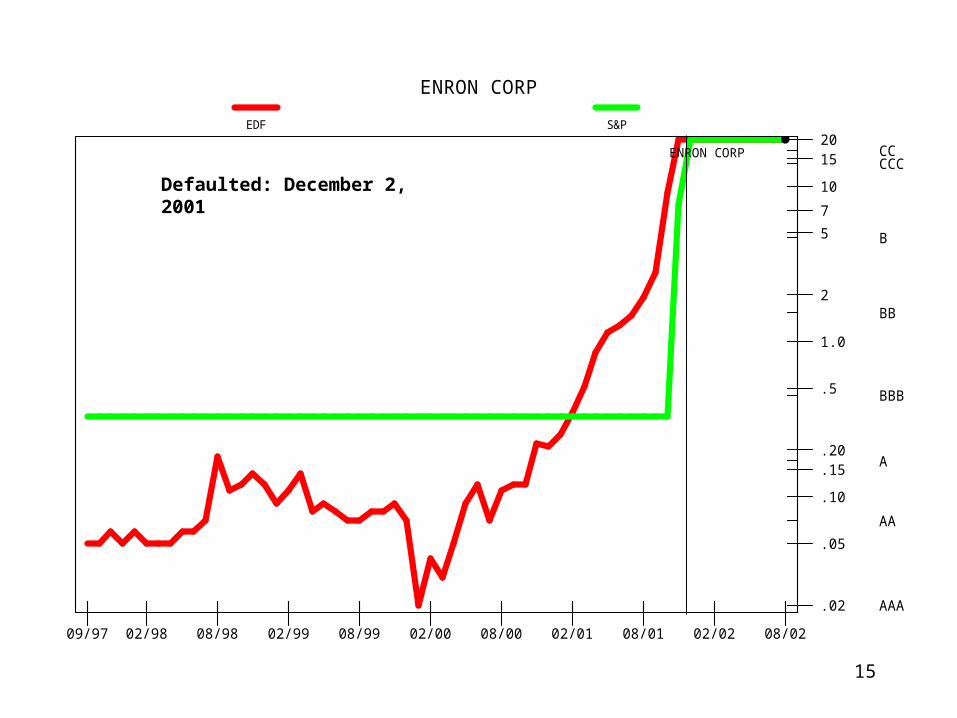
Example: Enron Corporation

• One of world’s largest energy companies– 22,000 employees, US $100 billion revenue– Six years on Forbes 100 best company list

• Declares bankruptcy December 2, 2001• Accounting fraud:

– First news in August 2001

14

15

ENRON CORP

.02

.05

.10

.15 .20

.5

1.0

2

5 7 10

15 20

AAA

AA

A

BBB

BB

B

CCC CC

09/97 02/98 08/98 02/99 08/99 02/00 08/00 02/01 08/01 02/02 08/02

ENRON CORP

EDF S&P

Defaulted: December 2, 2001

16

103

104

105

09/97 02/98 08/98 02/99 08/99 02/00 08/00 02/01 08/01 02/02 08/02

Credit Monitor®

N-ENRON CORP-AVL N-ENRON CORP-EVL N-ENRON CORP-DPT

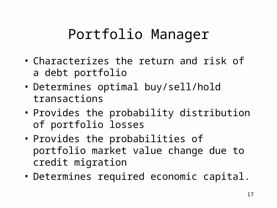
Portfolio Manager

• Characterizes the return and risk of a debt portfolio

• Determines optimal buy/sell/hold transactions• Provides the probability distribution of portfolio

losses• Provides the probabilities of portfolio market

value change due to credit migration• Determines required economic capital.

17

18

Correlation of defaults

• A loan defaults if the market value of borrower’s assets at loan maturity is less than the obligations due

• Borrowers’ asset values are correlated:– Dependence on common factors such as the

economy and the industry– Input-output interdependencies

• The correlations need to be taken into account in portfolio risk measurement.

19

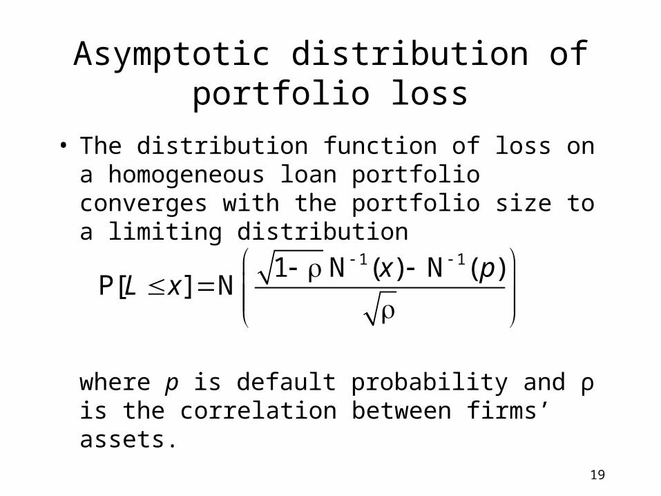
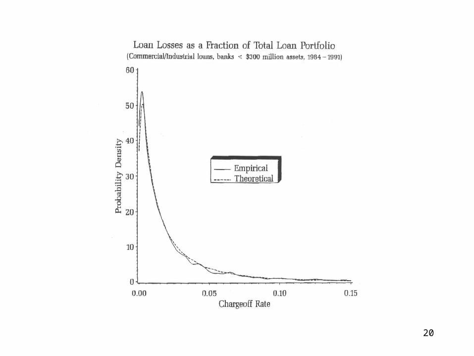
Asymptotic distribution of portfolio loss

• The distribution function of loss on a homogeneous loan portfolio converges with the portfolio size to a limiting distribution

where p is default probability and ρ is the correlation between firms’ assets.

1 11 N ( ) N ( )P[ ] N

x pL x

20

21

Actual portfolio

• Calculate the actual portfolio expected loss and variance of loss

• Approximate the portfolio loss distribution by the limiting distribution with the same first two moments

22

Determination of bank capital adequacy

• Bank rating corresponds to the probability of default for the bank:– AAA : 2 bp bank default probability– AA : 5 bp– A : 10 bp– BBB : 20 bp etc.

• To maintain a desired rating, the bank must have enough capital so that the probability of loss larger than capital is that corresponding to the rating.

23

Determining required capital

EL = 1%, ρ = .4

Percentage Cumulative

Loss Probability

5.00% 1.16%

6.00% 0.80%

7.00% 0.56%

8.00% 0.41%

9.00% 0.30%

10.00% 0.22%

11.00% 0.16%

12.00% 0.12%

12.62% 0.10%

13.00% 0.09%

14.00% 0.07%

15.00% 0.05%

24

Percentiles of the loss distribution, α = .999Average asset correlation

Average EDF 0.1 0.2 0.3 0.4 0.5 0.60.10% 0.52% 1.12% 1.90% 2.85% 4.01% 5.41%0.20% 0.90% 1.89% 3.13% 4.66% 6.54% 8.87%0.30% 1.24% 2.54% 4.14% 6.11% 8.52% 11.51%0.40% 1.55% 3.11% 5.03% 7.36% 10.18% 13.66%0.50% 1.84% 3.64% 5.82% 8.45% 11.61% 15.47%0.60% 2.11% 4.13% 6.55% 9.43% 12.87% 17.03%0.70% 2.37% 4.59% 7.21% 10.32% 14.01% 18.40%0.80% 2.63% 5.02% 7.84% 11.15% 15.03% 19.62%0.90% 2.87% 5.43% 8.42% 11.91% 15.97% 20.71%1.00% 3.10% 5.82% 8.98% 12.62% 16.83% 21.70%1.10% 3.33% 6.20% 9.50% 13.29% 17.63% 22.60%1.20% 3.55% 6.56% 10.00% 13.92% 18.38% 23.42%1.30% 3.76% 6.90% 10.47% 14.51% 19.07% 24.18%1.40% 3.97% 7.24% 10.93% 15.08% 19.73% 24.88%1.50% 4.17% 7.57% 11.36% 15.61% 20.34% 25.53%1.60% 4.37% 7.88% 11.78% 16.13% 20.92% 26.13%1.70% 4.57% 8.19% 12.19% 16.61% 21.47% 26.69%1.80% 4.76% 8.48% 12.58% 17.08% 21.99% 27.22%1.90% 4.95% 8.77% 12.95% 17.53% 22.48% 27.72%2.00% 5.13% 9.05% 13.32% 17.96% 22.95% 28.18%

25

Conclusions

• Mathematical finance can provide tools to quantify credit risk and the pricing of debt

• Quantitative techniques can be used to measure portfolio risk, optimize portfolio composition, determine required capital, and structure and price credit derivatives.