ESTIMATION OF RUNOFF OF AN UPPER CATCHMENT OF

AN EXISTING RESERVOIR BY SCS-CN METHOD, USING GIS

SOFTWARES

Under the guidance of Prof. Kalyan Kumar Bhar

BY - ADWAY DAS

ANIRBAN BANERJEE

PUNNAG SINHA SUMIT KUMAR DAS

INDIAN INSTITUTE OF ENGINEERING SCIENCEAND TECHNOLOGY, SHIBPUR

HOWRAH - 711103

FORWARD

I hereby forward the project titled “ESTIMATION OF RUNOFF OF AN UPPER CATCHMENT

OF AN EXISTING RESERVOIR BY SCS –CN METHOD USING GIS SOFTWARES” prepared

under guidance of Prof. Kalyan Kumar Bhar for the award of Bachelor of Engineering (Civil

Engineering) of Indian Institute of Engineering , Science & Technology , Shibpur.

(Prof. Kalyan Kumar Bhar)

Professor of Civil Engineering

IIEST,Shibpur IIEST , Shibpur

Date:-18/05/2015 Howrah-711103

INDIAN INSTITUTE OF ENGINEERING SCIENCE AND TECHNOLOGY, SHIBPUR

HOWRAH - 711103

CERTIFICATE OF APPROVAL

The foregoing seminar cum project titled “ESTIMATION OF RUNOFF OF AN UPPER

CATCHMENT OF AN EXISTING RESERVOIR BY SCS –CN METHOD USING GIS

SOFTWARES”, is hereby approved as a study of an engineering subject carried out & presented in a

manner satisfactorily to warrant its acceptance for the degree for which it has been submitted. It is

understood that , by this approval the undersigned do not necessarily endorse or approve any statement

made , opinion expressed or conclusion drawn there in but approved the project only for the purpose for

which it is submitted.

Board of project examiners:-

1.

2.

3.

ACKNOWLEDGEMENT

This result is the outcome of inspiration support, guidance, motivation, cooperation and facilities that

were extended to us their best and most by professors, lab assistants, students and our friends. At the

very onset, we express all our gratitude to our professors for stretching their liberal hands to help us for

undergoing such a worthy project on “ESTIMATION OF RUNOFF OF AN UPPER CATCHMENT

OF AN EXISTING RESERVOIR BY SCS –CN METHOD USING GIS SOFTWARES”.

We are also grateful to Prof. Kalyan Kumar Bhar for his continuous cooperation guidance, support and

generous interest in discussions during our project and it is his valuable advice that helped us making the

massive project.

We are also thankful to all the faculty member of CIVIL ENGINEERING department, as well as Mr.

Biman Sinha, PhD Research Scholar, for guiding and helping us through our problems.

----------------------------

ADWAY DAS (111104074)

---------------------------

ANIRBAN BANERJEE (111104061)

---------------------------

PUNNAG SINHA (111104059)

---------------------------

SUMIT KUMAR DAS (111104063)

TABLE OF CONTENTS: Sn. No. Description Pg. No.

1. Introduction 8

2. Literature review

2.1 SCS-CN method of estimating runoff volume

2.2 ESTIMATION OF CN

2.3Antecedent Moisture Condition (AMC)

2.4 Antecedent moisture conditions (AMC) for determining the value of CN

2.5 Calculation of CNI& CNIII from CNII

2.6 Runoff curve number CNII for hydrologic soil cover complexes (under AMC-

II condition).

2.7 SCS-CN equation for Indian condition

2.8 Procedure for estimating runoff volume from a catchment

10

10

11

11

12

12

12

.

13

13

3. Objective 14

4. Procedure

4.1 Creating a multi-band GeoTIFF from individual files using ArcGIS

4.2 Conducting supervised classification

4.2.1 Steps

4.2.1.1 Creating training samples

4.2.1.2 Preparing the Signature File

4.2.1.3 Performing a Supervised Classification

4.2.1.4 Reclassify

4.3 Aligning a non-georeferenced image to an existing georeferenced image

4.3.1 Steps

4.4 Digitalization of soil map

4.4.1Steps

4.5 Digital Elevation Modeling

4.5.1 Drainage Analysis

4.5.1.1 Fill Sinks

4.5.1.2 Flow Direction

4.5.1.3 Flow Accumulation

4.5.1.4 Stream Definition

15

15

15

15

15

16

16

17

17

18

19

19

21

21

21

21

21

21

4.5.1.5 Stream Segmentation

4.5.1.6 Catchment Delineation

4.5.1.7 Catchment Polygon Processing

4.5.1.8 Drainage Line Processing

4.5.1.9 Watershed Aggregation

4.6 CN Grid

4.6.1 Preparing land use data for CN Grid

4.6.2 Preparing Soil data for CN Grid

4.6.3 Merging of Soil and Landuse Data

4.6.4 Creating CN Look-up table

4.6.5 Creating CN Grid

4.7 Creation of impervious grid

4.8 Terrain Processing and HMS-Model Development using GeoHMS

4.8.1Dataset Setup

4.8.2 Creating New HMS Project

4.8.3 Basin Processing

4.8.4 River Profile

4.8.5 Extracting Basin Characteristics

4.8.6 River Length

4.8.7 River Slope

4.8.8 Basin Slope

4.8.9 Longest Flow Path

4.8.10 Basin Centroid

4.8.11 Basin Centroid Elevation

4.8.12 Centroidal Longest Flow Path

4.9 HMS Inputs/Parameters

4.9.1 Select HMS Processes

4.9.2 River Auto Name

4.9.3 Basin Auto Name

4.9.4 Sub-basin Parameters

4.9.5 CN Lag Method

21

22

22

22

22

23

23

23

23

24

24

25

26

26

26

27

28

28

28

28

29

29

30

30

30

31

31

31

32

32

32

4.10 HMS

4.10.1 Map to HMS Units

4.10.2 Check Data

4.10.3 HMS Schematic

4.10.4 Add Coordinates

4.10.5 Prepare Data for Model Export

4.10.6 Background Shape File

4.10.7 Basin Model

4.10.8 Meteorologic Model

4.11 HMS Project

4.11.1Steps

4.11.1.1Creating a Meteorologic Model

4.11.1.2Defining the Control Specifications

4.11.1.3 Editing the Parameters for Calculations

4.11.1.4 Executing the HMS Model

4.11.1.5 Viewing HMS Results

32

32

33

33

34

34

34

34

34

34

35

35

37

37

38

39

5. Results and Conclusion 40

6. References 41

1. INTRODUCTION:

Surface runoff is the flow of water that occurs when excess storm water, melt water, or other sources

flows over the earth's surface. This might occur because soil is saturated to full capacity, because rain

arrives absorb it, or because impervious areas (roofs and pavement) send their runoff to surrounding soil

that cannot absorb all of it. Surface runoff is a major component of the water cycle. It is the primary

agent in soil erosion by water.

Factors affecting surface runoff can be broadly classified into two main categories: meteorological

factors and physical factors.

Meteorological factors affecting surface runoff include:

1. Type of precipitation (rain, snow, sleet, etc.)

2. Rainfall intensity

3. Rainfall amount

4. Rainfall duration

5. Distribution of rainfall over the watersheds

6. Direction of storm movement

7. Other meteorological and climatic conditions that affect evapotranspiration, such as temperature,

wind, relative humidity, and season.

Physical factors affecting surface runoff include:

1. Land use

2. Vegetation

3. Soil type

4. Drainage area

5. Basin shape

6. Elevation

7. Slope

8. Topography

9. Direction of orientation

10. Drainage network patterns

11. Ponds, lakes, reservoirs, sinks, etc. in the basin, which prevent or alter runoff from continuing

downstream

Proper estimation and calculations of surface runoff is of prime importance to identify the maximum

discharge that drains into the reservoir. This, in turn, would help to identify, calculate and check the

design height of the dam that is to be built or modified. The need for modification of height might arise

due to change in permeability and infiltration of the soil in the basin, as well as the change in soil use in

the region.

Conventional method off runoff estimation is expensive, time consuming and difficult process and these

methods of runoff measurement are not easy for hilly and inaccessible terrains. Remote sensing

technology can augment the conventional methods to a great extent in rainfall-runoff studies. The role of

remote sensing in runoff calculation is generally provides a source of input data or as an aid for

estimation equation coefficients and model parameters. Experiences has shown that satellite data can be

interpreted to drive thematic information on land use, soil, vegetation, drainage, etc which combined

with conventionally measured climate parameter and topographic parameters height contour slope,

provide the necessary inputs to the rainfall-runoff models. The information extracted from remote

sensing and other sources can be stored as a georeferenced data base in geographical information system

(GIS).

The soil conservation service curve number (SCS-CN) method is widely used for predicting direct

runoff volume for a given rainfall event. This method is originally developed by the US department of

agriculture, soil conservation service and documented in detail in the “National Engineering Handbook”.

The curve number method (SCS, 1992) also known as the hydrologic soil cover complex method is a

versatile and widely used procedure for runoff estimation.

The main reason for its success is that it accounts for many of the factor affecting runoff generation

including soil type, land use and treatment surface condition, and antecedent moisture condition,

incorporating them in a single CN parameter. Furthermore it is the only methodology that features

readily grasped and reasonably well documented environmental inputs and it is a well-established

method widely accepted for use in United States and other consider the impact of rainfall intensity and

its temporal distribution. It does not effect of spatial scale.

In the present study, attempt will be made for estimation of runoff from a catchment using SCS (soil

conservation services) curve number model utilizing remote sensing and GIS technique.

1. Literature review The SCS-CN method has been widely used to compute direct surface runoff. It originated from the

proposal of Sherman (1949) on plotting direct runoff versus storm rainfall. The subsequent work

Mockus (1949) on estimated of surface runoff for ungauged stations using the soil information, rainfall,

storm, duration and average annual temperature.

The graphical procedure of Andrews (1982) for estimating runoff from rainfall for combination of soil

texture and type of amount of vegetation cover and conservation practices, also known as soil vegetation

land use (SVL).

Extensive work has been done to estimate discharge in river and the relevant literature review is given

below McCuen (1982) Hawkins (1993), Steenhuisetal (1995), Bonta (1997), Mishra and Singh has done

appreciable work in this field. Besides them Stuebe and Sahuet.al (2007) has done appreciable work in

this field.

SCS-CN method in their analysis Bhuyan et al (2003) studied event based watershed scale antecedent

moisture condition (AMC) values to adjust field-scale CNs, and to identify the hydrological parameters

that provide the best estimate of AMC. Patiletal (2008) has done work in this field using GIS based

interface selected site.

2.1SCS-CN method of estimating runoff volume

The first hypothesis equates the ratio of the amount of direct surface runoff Q to the total rainfall P (or

maximum potential surface to the runoff) with the ratio of the amount of infiltration Fc amount of the

potential maximum retention S. The second to the potential hypothesis relates the initial abstraction I

maximum retention. Thus the SCS-CN method consisted of the following equation.

Water balance equation:

P=Ia+Fc+Q Equation 2.1

Proportional equality hypothesis

Q/(P-Ia)=Fc/S Equation 2.2

Ia-S hypothesis

Ia=λs Equation 2.3

Where,P is the total rainfall. I the initial abstraction, Fc the cumulative infiltration excluding Ia, Q the

direct runoff, S= potential maximum retention or infiltration and the regional parameter dependent on

geologic and climatic factors (0.1<<0.3).

Solving equations,

Q=(P-Ia)^2/(P-Ia+S)

Q=(P-λs)^2/(P-(λ-1)S)

The relation between Ia and S was developed by analyzing the rainfall and runoff data from

experimental small watersheds and is expressed as Ia=0.2S. Combining the water balance equation and

proportional equality the SCS-CN method is represented as Q=(P-0.2S)^2(P+0.8S)

The potential maximum retention storage is related to a CN, which is a function of land use, land

treatments, soil type and antecedent moisture condition of water shed. The CN is dimensionless and its

value from 0 to 100. The S-Value in mm can be obtained from CN by using the relationship.

2.2 ESTIMATION OF CN:

In determining the CN the hydrological classification is adopted. Here soils are classified into four

classes A,B,C,D based on the infiltration and other characteristics. The important soil characteristics the

influence the hydrological classification of soils are effective depth of soil, average clay content,

infiltration characteristics and the permeability.

Table 1: Classification of soil

Classification

Type of soil

Group A-(Low Runoff

Potential)

Soil with high infiltration capacity, even when thoroughly wetted. Sand and gravel

deep and well drained

Group B-(Moderately Low

Runoff Potential)

Soil with moderate infiltration rate when thoroughly wetted. Moderately deep to

deep and moderately well to well drained with moderately fine to moderately

coarse texture.

Group C-(Moderately

High Runoff Potential)

Soil with slow infiltration rate when thoroughly wetted. Usually have a layer that

impedes vertical drainage or have a moderately fine to fine texture.

Group D-(High Runoff

Potential)

Soil with slow infiltration rate when thoroughly wetted. Chiefly clay with a high

swelling potential, soil with a high permanent water table, soil with a clay layer or

near the surface.

2.3Antecedent Moisture Condition (AMC)

Antecedent Moisture condition is the preceding relative moisture of the pervious surfaces prior to the

rainfall event. This is also referred to as Antecedent Runoff Condition (ARC). Antecedent Moisture is

considered to be low when therehas been little preceding rainfall and high when therehas been

considerable preceding rainfall prior to the modelled rainfall event.

For the purpose of practical application three levelsof AMC are recognized by SCS as follows:-

AMC-I: Soils are dry but not wilting point. Satisfactory cultivation has taken place.

AMC-II: Average condition.

AMC-III: Sufficient rainfall occurred within past 5 days.

2.4 Antecedent moisture conditions (AMC) for determining the value of CN

Table 2: AMC values

AMC TYPE

DORMANT SEASON

(TOTAL RAIN IN

PREVIOUS 5 DAYS)

GROWING SEASON

(TOTAL RAIN IN

PREVIOUS 5 DAYS)

I Less than 13 mm Less than 36 mm

II 13 to 28 mm 36 to 53 mm

III Greater than 28 mm More than 53 mm

2.5 Calculation of CNI& CNIII from CNII

The conversion of CNII to other two AMC conditions can be made through the use of following

correlations:

For AMC-I: CNI = CNII / (2.281 – 0.01281CNI )

For AMC-III: CNIII = CNII / (0.427 + 0.00573CNII )

Where, CNII ranges from 55 to 95

2.6 Runoff curve number CNII for hydrologic soil cover complexes (under AMC- II condition)

Table 3: Runoff curve number CNII

Land Cover Hydrological Soil Group

Treatment

or Practice

Hydrologic

Condition A B C D

Cultivated Straight

Row 76 86 90 93

Cultivated Contoured Poor 70 79 84 88

Good 65 75 82 86

Cultivated

Contoured

And Poor 62 71 77 81

Terraced Good 67 75 81 83

Cultivated Bunded Poor 59 69 76 79

Good 95 95 95 95

Cultivated Paddy

39 53 67 71

Orchards

With Understory Cover 41 55 69 73

Without Understory

Cover 26 40 58 61

Forest

Dense

28 44 60 64

Open 33 47 64 67

Scrub 68 79 86 89

Pasture

Poor

49 69 79 84

Fair

39 61 74 80

Good

71 80 85 88

Wasteland

73 83 88 90

Roads

77 86 91 93

2.7SCS-CN EQUATION FOR INDIAN CONDITION:

Value of λ varying the range .1<λ<4 has been documented in a number of studies from various

geographical location, which includes USA and many other countries. For use in INDIA conditions λ=1

and 3 subjected to certain constants of soil type and AMC type has been recommended as below-

Q= ((P-0.1S)^2)/(P+0.9S)

Valid for block soil under AMC OF TYPE II AND III

Q=((P-0.3S)^2)/(P+0.7S)

AMC type of I and for all other soil having AMC of type I,II,III.

2.8 PROCEDURE FOR ESTIMATING RUNOFF VOLUME FROM A CATCHMENT:-

Land use/cover information of the catchment under study is derived based on interpretation of multi

season satellite images. It is highly advantageous if the GIS database of the catchment is prepared and

land use/ cover is linked to it. The soil information of catchment is obtained by using soil map prepared

NATIONAL BUREAU of soil survey and land use planning (NBBS&LUP)(1996). Soil data relevant to

the catchment is indentified and appropriate hydrological soil classification is made and the spatial form

the data is stored in GIS database. Available rainfall data of various rain gauge station in and around the

catchment is collected, screened for consistency and accuracy linked to the GIS database. For

reasonable estimate of catchment yield it is desirable to have a rainfall record for the last 25 yrs

duration. Appropriate area weighted CN value is established by adequate consideration of spatial

variation of land/cover and soil types. Using the relevant SCS-CN equation sequentially with the rainfall

data, the corresponding daily runoff series divided for each cell. From this, needed weekly/

monthly/annual runoff time series is derived.

3. OBJECTIVE:

The objective of this project is to use GIS software (ArcMap 10) to calculate the runoff in the upper

catchment of an existing reservoir. In this project, we focus solely on the physical factors that affect the

runoff, and leave out the meteorological factors. We aim to determine the runoff rates across different

regions of the delineated catchment area for the reservoir, by using the GIS software to compile and

analyze satellite data as well as soil data obtained from NBSS Publication 13 (Sehgalet al., 1987, second

edition).

Thus, the objective of the project can be jotted down to the following sub-objectives:

To obtain the satellite data for the catchment region, and to preprocess these satellite images

To perform a supervised classification of the Landsat image based on the type of land use

To prepare the soil layer clip with proper georeferenced points on the available soil map

To create a union of the land use map and the processed soil data to create the CN grid for the

catchment

STUDY AREA:

The study area for this project is the upper catchment of the Tilaiya Reservoir, Bihar, India.

4. PROCEDURE:

4.1 Creating a multi-band GeoTIFF from individual files using ArcGIS

2. Combine all bands of satellite image ArcToolbox – Data Management Tools – Raster –

Raster Processing – Composite Bands

Enter input rasters (bands) and output raster

3. Change the projection of output raster to WGS-1984, UTM Zone 45N

ArcToolBox – Data Management Tools – Projectionn and Transformation – Raster –

Project Raster

Output coordinate system: WGS-1984, UTM Zone 45N

4. Extract study area from satellite image

ArcToolbox – Spatial Analyst Tool – Extraction – Extract by mask

Enter input raster, mask data

Input raster and mask data must be in same projection system

5. Change band combination system to 3:2:1 (R:G:B) Right click on Raster – properties -

symbology

4.2 Conducting supervised classification:

In comparison to computer-controlled unsupervised classification, the supervised classification process

gives a much better control. In this process, pixels are selected such that they represent recognizable

patterns. Knowledge of the data, the classes desired, and the algorithm to be used is required before

beginning the selection of training samples. By identifying patterns in the imagery, we can "train" the

computer system to identify pixels with similar characteristics. By setting priorities for these classes, we

supervise the classification of pixels as they are assigned to class values. If the classification is accurate,

then each resulting class corresponds to a pattern that has been originally identified.

4.2.1 Steps:

4.2.1.1 Creating training samples: We are going to start with identifying areas for individual

classes. For this, we need to use the image classification toolbar, which is shown in the figure

below:

Fig 1: Image Classification Toolbar

Left-clicking on the down arrow next to Draw Polygon gives us three options to select regions on the

image– Draw Polygon, Draw Rectangle, and Draw Circle. We make use of the Draw Polygon option

to draw our training samples. The Training Sample Manager gives the list of the Classes thus

demarcated.

Fig 2: Training Sample Manager (left) an d Scatterplot (right)

Scatterplots plot the pixel values of our training data in one band against those of another. Viewed as

scatterplots, the points should not overlap if the training samples represent different spectral classes. As

many training sets as possible, comprising maximum pixels should be taken into consideration while

creating the training samples to ensure proper classification of the region.

4.2.1.2 Preparing the Signature File: We have one last step before performing the

classification. We need a signature file created from our training data. Highlight all the rows in

ourTraining Sample Manager and left-click on the Create a signature file button, and save the

signature file.

4.2.1.3 Performing a Supervised Classification: Left-click on the down arrow next to

classification and click on Maximum Likelihood Classification. We need to use the above saved

signature file as the input for this step, and the result is shown in the figure below.

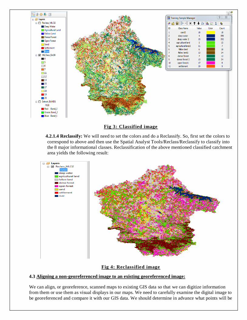
Fig 3: Classified image

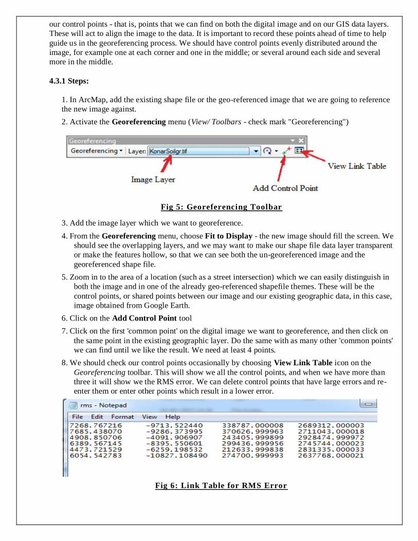
4.2.1.4 Reclassify: We will need to set the colors and do a Reclassify. So, first set the colors to

correspond to above and then use the Spatial Analyst Tools/Reclass/Reclassify to classify into

the 8 major informational classes. Reclassification of the above mentioned classified catchment

area yields the following result:

Fig 4: Reclassified image

4.3 Aligning a non-georeferenced image to an existing georeferenced image:

We can align, or georeference, scanned maps to existing GIS data so that we can digitize information

from them or use them as visual displays in our maps. We need to carefully examine the digital image to

be georeferenced and compare it with our GIS data. We should determine in advance what points will be

our control points - that is, points that we can find on both the digital image and on our GIS data layers.

These will act to align the image to the data. It is important to record these points ahead of time to help

guide us in the georeferencing process. We should have control points evenly distributed around the

image, for example one at each corner and one in the middle; or several around each side and several

more in the middle.

4.3.1 Steps:

1. In ArcMap, add the existing shape file or the geo-referenced image that we are going to reference

the new image against.

2. Activate the Georeferencing menu (View/ Toolbars - check mark "Georeferencing")

Fig 5: Georeferencing Toolbar

3. Add the image layer which we want to georeference.

4. From the Georeferencing menu, choose Fit to Display - the new image should fill the screen. We

should see the overlapping layers, and we may want to make our shape file data layer transparent

or make the features hollow, so that we can see both the un-georeferenced image and the

georeferenced shape file.

5. Zoom in to the area of a location (such as a street intersection) which we can easily distinguish in

both the image and in one of the already geo-referenced shapefile themes. These will be the

control points, or shared points between our image and our existing geographic data, in this case,

image obtained from Google Earth.

6. Click on the Add Control Point tool

7. Click on the first 'common point' on the digital image we want to georeference, and then click on

the same point in the existing geographic layer. Do the same with as many other 'common points'

we can find until we like the result. We need at least 4 points.

8. We should check our control points occasionally by choosing View Link Table icon on the

Georeferencing toolbar. This will show we all the control points, and when we have more than

three it will show we the RMS error. We can delete control points that have large errors and re-

enter them or enter other points which result in a lower error.

Fig 6: Link Table for RMS Error

9. When we have completed the georeferencing process, we can create a permanently georeferenced

image by choosing Rectify from the Georeferencing Specify a name and location for the new

image. The result will be a .tif image and a .tfw world file, which tells ArcMap where in the

world this image is now located.

10. With this georeferenced image, we can now digitize new features from the map.

4.4 Digitalization of soil map:

Digitizing in GIS is the process of “tracing”, in a geographically correct way, information from

images/maps. The process of georeferencing relies on the coordination of points on the scanned image

(data to be georeferenced) with points on a geographically referenced data (data to which the image will

be georeferenced). By “linking” points on the image with those

same locations in the geographically referenced data we will create a polynomial transformation that

converts the location of the entire image to the correct geographic location.

4.4.1Steps:

1. Creating an empty shapefile. Open ArcCatalog. We are going to create a new shapefile that

we can edit in ArcMap. Go to New, click the Shapefile to open the Create New

Shapefilewindow.

2. The editor toolbar is first opened. Clicking on the Start Editing option results in the opening

of a toolbar as shown in the figure.

3. We use the Polygon option under the Construction Tools to create the polygons along the

lines of individual soil types demarcated in the .tif image.

Fig 7: Editor Toolbar (left), on clicking Start Editing opens the window (on right)

4. When all the polygons have been drawn, click the Save Edits option in the Editor toolbox to

save the changes, and then click on Stop Editing.

Fig 8: Digitized image (left) and its corresponding Attribute Table (right)

The result after digitalization of the soil types in and around the reservoir looks as described in figure.

Right clicking on the layer gives us the Open Attribute Table which gives the list of the polygons

selected, the Shape length of the polygon boundaries, and the Shape Area of the individual polygons.

Fig 9: Digitized image clipped to consider only Project Area (left) and its

corresponding Attribute Table

Next, we need to clip these digitized polygons such that we deal with only those regions that fall under

our project catchment area. The result obtained is shown in figure. Right clicking on the layer gives us

the Open Attribute Table which gives the list of the polygons selected, the Shape length of the polygon

boundaries, and the Shape Area of the individual polygons. Here, we need to add a few more columns

in the Attribute Table, to attach the soil type to each of these digitized images.

For this, we click on the Stop Editing option on the Editor Toolbox. This allows us to Add Field in the

attribute table. We need to add 5 columns to determine the soil code type. This data needs to be filled

manually, using the information available with us.

4.5 Digital Elevation Modelling:

4.5.1.1 Drainage Analysis

4.5.1.1 Fill Sinks

Select Preprocessing – Fill Sinks. Press OK.

The output Hydro DEM is Fil

4.5.1.2 Flow Direction

Select Preprocessing – Flow Direction

Confirm that the input Hydro DEM is Fil. The output Flow Direction Grid is Fdr.

Press OK

Fig 10: Result after Fill Sinks (left) , after Flow Direction (middle), and after Flow

Accumulation (right)

4.5.1.3 Flow Accumulation

Select Preprocessing – Flow Accumulation

Confirm that the input Flow Direction is Fdr. The outpur Flow Accumulation Grid is Fac

Press OK

4.5.1.4 Stream Definition

Select Preprocessing – Stream Definition

Confirm that the input Flow Accumulation Grid is Fac. The output Stream Grid is Str.

Accept the default Stream Threshold and Press OK.

4.5.1.5 Stream Segmentation

Select Preprocessing – Stream Segmentation

Confirm that the input Flow Direction Grid is Fdr and Stream Grid is Str. The output

Stream Link Grid is StrLnk.

Press OK.

Fig 11:Result after Stream Definition(left) and Stream Segmentation (right)

4.5.1.6 Catchment Delineation

Select Preprocessing - Catchment Grid Delineation

Confirm that the input Flow Direction Grid is Fdr and Link Grid is StrLnk. The output

Catchment Grid is Cat.

Press OK.

4.5.1.7 Catchment Polygon Processing

Select Preprocessing – Catchment Polygon Processing

Confirm that the input Catchment Grid is Cat. The output Catchment layer is Catchment.

Press OK

Fig 12: Result after Catchment Delineation (left) and Catchment Polygon Processing

(right)

4.5.1.8 Drainage Line Processing

Select Preprocessing – Drainage Line Processing

Confirm that the input Stream Link Grid is StrLnk and Flow Direction Grid is Fdr. The

output Drainage Line is DrainageLine.

Press OK.

4.5.1.9 Watershed Aggregation

Select Preprocessing – Adjoint Catchment Processing

Confirm that the input Drainage Line is DrainageLine and Catchment is Catchment. The

output Adjoint Catchment is AdjointCatchment

Press OK.

Fig 13: Result of Drainage Line Processing (left) and Watershed Aggregation (right)

4.6 CN Grid:

4.6.1 Preparing land use data for CN Grid

1. Open the Reclassified Land use data.

2. The final step in processing land use data is converting the reclassified land use grid into a

polygon feature class which will be merged with soil data later. In ArcToolbox, Click on

Conversion Tools - From Raster - Raster to Polygon.

a. Confirm the Input raster is the existing reclassified file, the Field is Value, output

geometry type is Polygon, and save the Output features as a .shpfile

b. Click OK.

3. Save the map document.The processing of land use data for preparing curve number grid is

over.

4.6.2 Preparing Soil data for CN Grid

The soil Data has already been prepared for use in the CN Grid in the previous procedures.

4.6.3 Merging of Soil and Landuse Data

1. To merge/union soil and landuse data, Click ArcToolbox - Analysis Tools - Overlay Union

tool. Select the SoilClipand the Landuse_polygon as input features, name the output feature

class in the same geodatabase, leave the default options, and click OK.

2. This process will take few minutes, and the resulting Joint feature class will be added to the

map document. Save the map document.

3. The result of union/merge features inherit attributes from both feature classes that are used as

input. However, if the outer boundaries of input feature classes do not match exactly, the

resulting merged feature class usually will have features that will have attributes from only

one feature class because the other feature do not exist in this area. These features are usually

referred to as “slivers”. If we open the attribute table for this merged feature class, we will

find that there are several sliver polygons in this feature class that have attributes only from

the LandUse polygon and the soil attributes are empty, and vice versa as shown below:

Fig 14: Attribute Table obtained on Merging Soil and Landuse Data

The slivers are denoted by either -1 or 0.

4. Start the Editor. Select all the features that have “FID_...” = -1 and “FID_...” = 0 and delete

them. Save our edits, stop the Editor, and save the map document.

4.6.4 Creating CN Look-up table

1. Create a table named CNLookUp. In ArcCatalog, select Data Management Tools – Table -

Create Table. Once the table is created create the following fields in it:

a. LUValue (type: short integer)

b. Description (type: text)

c. A (type: short integer)

d. B (type: short integer)

e. C (type: short integer)

f. D (type: short integer)

2. Now start the Editor to edit the newly created CNLookUp table, and populate it using the

following data table:

Table 4: CN LookUp Table

Description of

Land Use

Hydrologic Soil Group

A B C D

Agriculture 67 76 83 86

Fallow Land 54 70 80 85

Settlement 57 72 81 86

Dense Forest 30 55 70 77

Open Forest 36 60 73 79

Sand 77 86 91 94

River 97 97 97 97

Deep Water 100 100 100 100

3. Columns A/B/C/D store curve numbers for corresponding soil groups for each land use

category. These numbers are obtained from SCS TR55 (1986). Save the edits and stop the

Editor. Save the map document.

4.6.5 Creating CN Grid

1. Activate the HEC-GeoHMS Project View toolbar

2. HEC-GeoHMS uses the merged feature class and the lookup table to create the curve

number grid.

3. Create a field named LandUse (type: short integer), and populate it by equating it to

GRIDCODE.

4. On the HEC-GeoHMS Project View toolbar, click on Utility - Create Parameter Grids.

Choose the lookup parameter as Curve Number , Click OK, and then select the inputs

as:HydroDEM for Hydro DEM, merged soil and land use for Curve Number Polygon,

CNLookUp table for Curve Number Lookup, and leave the default CNGrid name for the

Curve Number Grid.

5. Save the map document.

4.7 Creation of impervious grid

1. Convert land use map (grid) into a polygon feature class.

ArcToolbox Conversion Tools From Raster Raster to polygon (Field Value)

2. Add a new field ImpPctin the attribute table of land use polygon shapefile.

3. GridCodefield contains different land use classes. Insert percent impervious area value in

ImpPctfield based on land use classes.

(save the attribute table in .dbf format. Open the .dbf file in Excel. Insert percent impervious

values in the column, and save it in the .dbf format)

4. Open the corrected .dbf file in ArcGis

5. Join .dbf fields with the attribute table of land use polygon shape file.

6. Use Field Calculator to populate ImpPctfield of polygon file (same as ImpPctfield of .dbf file)

Fig 15: Attribute table of shapefile polygon (left) and Data Source for Percentage

Impervious Area (right)

7. Create percent impervious area grid (raster based on ImpPct field of land use polygon)

ArcToolbox – Conversion Tools – to Raster – Feature to Raster (Input Features:

LandUse_polygon, Field: ImpPct)

Fig 16: Raster layer obtained of Impervious Grid

4.8 Terrain Processing and HMS-Model Development using GeoHMS

4.8.1Dataset Setup

1. SelectHMS Project Setup - Data Management on the HEC-GeoHMS Main View toolbar.

Confirm/define the corresponding map layers in the Data Management window as shown

below:

Fig 17: Data Management Window

2. ClickOK.

4.8.2 Creating New HMS Project

1. Click on Project Setup - Start New Project. Confirm ProjectArea for ProjectArea and

ProjectPoint for ProjectPoint, and click OK.

Fig 18: Creating New HMS Project

2. This will create ProjectPoint and ProjectArea feature classes.

3. If we click on Extraction Method drop-down menu, we will see another option A new

threshold which will delineate streams based on this new threshold for the new project.

Accept the default original stream definition option. Choose the outside MainView

Geodatabase for Project Data Location, and browse to our working directory where

RawDEM.mxd is stored. Click OK.

4. Click OK on the message regarding successful creation of the project. We will see that new

feature classes ProjectArea and ProjectPoint are added to ArcMap’s table of contents. These

feature classes are added to the same geodatabase.

5. Next Zoom-in to define the watershed outlet

6. Select the Add Project Points tool on the HEC-GeoHMS toolbar, and click on the

downstream outlet area to define the outlet point as shown below as red dot.

7. Accept the default Point Name and Description (Outlet), and click OK. This will add a point

for the watershed outlet in the ProjectPoint feature class. Save the map document.

Fig 19: Adding Project Points

8. Next, select HMS Project Setup - Generate Project. This will create a mesh (by delineating

watershed for the outlet in Project Point)

9. Confirm the layer names for the new project (leave default names for Subbasin, Project

Point, River and BasinHeader), and click OK.

Fig 20: Generation of Project

4.8.3 Basin Processing

The basin processing menu has features such as revising sub-basin delineations, dividing basins, and

merging streams.

4.8.4 River Profile

1. The River Profile tool allows displaying the profile of selected river reach (es). If the river

slope changes significantly over the reach length, it may be useful to split the river/watershed

at such a slope change.

2. Select the River Profile tool, and click on any river segment that we are interested in

inspecting. Confirm the layers in the next window, and click OK.

3. This will invoke a dockable window in ArcGIS at the bottom that will display the profile of

the selected reach.

4. If we click at a point along the profile, a corresponding point showing its location on the river

reach will be added to the map display (shown below as red dot).

Fig 21: River selected, and its profile

5. If we want to split the river segment at the selected point, we can just right click on the point

inside the dockable window and split the river. If we want to split the sub-basin at the point

displayed in the map, we can use the subbasin divide tool, and click at the point displayed on

the map. We will not split any river segments in this exercise.

6. Close the dockable window, and save the map document.

4.8.5 Extracting Basin Characteristics

The basin characteristics menu in the HEC-GeoHMS Project View provide tools for extracting

physical characteristics of streams and sub-basins into attribute tables.

4.8.6 River Length

This tool computes the length of river segments and stores them in RiverLen field. Select

Characteristics - River Length. Confirm the input River name, and click OK.

Fig 22: River Length Tool

4.8.7 River Slope

This tool computes the slope of the river segments and stores them in Slp field. Select Basin

Characteristics - River Slope. Confirm inputs for RawDEM and River, and click OK.

Fig 23: River Slope Tool

4.8.8 Basin Slope

This tool computes average slope for sub-basins using the slope grid and sub-basin polygons.

Add wshslopepct (percent slope for watershed) grid to the map document. Select Characteristics -

Basin Slope. Confirm the inputs for Subbasin and Slope Grid , and click OK.

Fig 24: Basin Slope Tool

After the computations are complete, the BasinSlope field in the input Subbasin feature class is

populated.

4.8.9 Longest Flow Path

This will create a feature class with polyline features that will store the longest flow path for each sub-

basin. Select Characteristics - Longest Flow Path. Confirm the inputs, and leave the default output

name LongestFlowPath unchanged. Click OK.

Fig 25: Longest Flow Path Tool

A new feature class storing longest flow path for each sub-basin is created as shown below:

Fig 26: Subbasins created

Fig 27: Attribute Table of the generated Subbasins

4.8.10 Basin Centroid

This will create a Centroid point feature class to store the centroid of each sub-basin. Select

Characteristics - Basin Centroid. Choose the default Center of Gravity Method, input Subbasin, leave

the default name for Centroid. Click OK.

Fig 28: Basin Centroid Toolbar (left) and Subbasins with respective centroids (right)

A point feature class showing centroid for each sub-basin is added to the map document.As centroid

locations look reasonable, we will accept the center of gravity method results, and proceed. Save the

map document.

4.8.11 Basin Centroid Elevation

This will compute the elevation for each centroid point using the underlying DEM. Select

Characteristics - Centroid Elevation Update. Confirm the input DEM and centroid feature class, and

click OK.

Fig 29: Basin Centroid Elevation Toolbar

After the computations are complete, open the attribute table of Centroid to examine the Elevation field.

4.8.12 Centroidal Longest Flow Path

Select Characteristics - Centroidal Longest Flow Path. Confirm the inputs, and leave the default name

for output Centroidal Longest Flow Path, and Click OK.

Fig 30: Centroidal Longest Flowpath Toolbar

This creates a new polyline feature class showing the flowpath for each centroid point along longest

flow path. Save the map document.

4.9 HMS Inputs/Parameters

The hydrologic parameters menu in HEC-GeoHMS provides tools to estimate and assign a

number of watershed and stream parameters for use in HMS. These parameters include SCS curve

number, time of concentration, channel routing coefficients, etc.

4.9.1 Select HMS Processes

Select Hydrologic Parameters - Select HMS Processes. Confirm input feature classes for

Subbasin and River, and click OK. Choose SCS for Loss Method (getting excess rainfall from total

rainfall), SCS for Transform Method (for converting excess rainfall to direct runoff), None for

Baseflow Type, and Muskingum for Route Method (channel routing). Click OK.

Fig 31: Select HMS Processes Window

4.9.2 River Auto Name

This function assigns names to river segments. Select Parameters - River Auto Name. Confirm the

input feature class for River, and click OK.

Fig 32: River Auto Name Toolbar

4.9.3 Basin Auto Name

This function assigns names to sub-basins. Select ParametersBasin Auto Name. Confirm the input feature class for sub-basin, and click OK.

Fig 33: Basin Auto Name Toolbar

4.9.4 Sub-basin Parameters

1. Add cngrid (curve number grid) from Layers folder to the map document. Select Hydrologic

ParametersSubbasin Parameters. You will get a menu of parameters that you can assign. Uncheck all parameters and check BasinCN as shown below, and Click OK.

Fig 34: Subbasin Parameters From Raster Window

2. Confirm the inputs for Subbasin and Curve Number Grid, and click OK.

3. After the computations are complete, you can open the attribute table for subbasin, and see that a field named BasinCN is populated with average curve number for each sub-basin. Close the

attribute table, and save the map document.

Fig 35: Attribute table with populated BasinCN column

4.9.5 CN Lag Method

Select Hydrologic ParametersCN Lag Method. This function populates the BasinLag field in the

subbasin feature class with numbers that represent basin lag time in hours. Save the map document.

4.10 HMS The HMS menu has tools for creating input files for HEC-HMS.

4.10.1 Map to HMS Units

This tool is used to convert units. Click on HMSMap to HMS Units. Confirm the input files, and click

OK.

Fig 36: Select unit type for HMS Model

4.10.2 Check Data

This tool will verify all the input datasets. Select HMSCheck Data. Confirm the input datasets to be

checked, and click OK. You should get a message after the data check saying the check data is completed successfully as shown below.

Fig 37: Check data Toolbar (left), Checking Summary (right)

4.10.3 HMS Schematic

Select HMSHMS Schematic. Confirm the inputs, and click OK.

Fig 38: HMS Schematic Toolbar (left) and HMS Link (right)

Two new feature classes HMS Link and HMSNode will be added to the map document. After the schematic

is created, you can get a feel of how this model will look like in HEC-HMS by toggling/switching between

regular and HMS legend. Select HMSToggle HMS LegendHMS Legend

Fig 39: HMS Node

4.10.4 Add Coordinates This tool attaches geographic coordinates to features in HMSLink and HMSNode feature classes. This is useful for exporting the schematic to other models or programs without loosing the geospatial information.

Select HMSAdd Coordinates. Confirm the input files, and click OK.

4.10.5 Prepare Data for Model Export Select HMSPrepare Data for Model Export. Confirm the input Subbasin and River files, and click OK.

This function allows preparing subbasin and river features for export.

4.10.6 Background Shape File Select HMSBackground Shape File. This function captures the geographic information (x,y) of the

subbasin boundaries and stream alignments in a text file that can be read and displayed within HMS. Two

shapefiles: one for river and one for sub-basin are created in the project folder. Click OK on the process completion message box.

4.10.7 Basin Model Select HMSBasin Model File. This function will export the information on hydrologic elements (nodes and links), their connectivity and related geographic information to a text file with .basin extension. The

output file project name with .basin extension is created in the project folder. Click OK on the process

completion message box.

You can also open the .basin file using Notepad and examine its contents.

Fig 40: .Basin file opened using Notepad

4.10.8 Meteorologic Model We do not have any meteorologic data (temperature, rainfall etc) at this point. We will only create an empty

file that we can populate inside HMS. Select HMSMet Model FileSpecified Hyetograph. The output

file project name with .met extension is created in the project folder. Click OK on the process completion message box. You can also open the .met file using Notepad and examine its contents.

4.11 HMS Project This function copies all the project specific files that you have created (.met, .map, and .met) to a

specified directory, and creates a .hms file that will contain information on other files for input to HMS.

Select HMSCreate HMS Project. Provide locations for all files. Even if we did not create a gage file,

there will be a gage file created when the met model file is created. Give some name for the Run, and leave the default information for time and time interval unchanged. This can be changed in HEC-HMS based on

the event you will simulate. Click OK

Fig 41: Creating HMS Project

This leads to the creation of the following layers in HEC GIS: one each for Basin Models, Meteorologic

Models, Control Specifications, and Time-Series Data. The Outlet3 sub layer created is automatically filled

with the number of subbasins created in the previous steps, by default.

Fig 42: Layers created on opening a new HMS project

4.11.1Steps:

4.11.1.1Creating a Meteorologic Model a. This is done by specifying a time series of rainfall at a Rainfall gauge, and associating

this gauge with each individual sub-basin or all sub-basins. If you click on the time series

folder in the Watershed Explorer, you will see that there is a gage associated with each sub-basin. Let’s remove these gauges, and use only one rainfall gauge for the entire

catchment area.

b. Click on Components - Time Series Data Manager, and create a new Gage called Gage

D. Close the Time-Series Data Manager. c. Next, in the Watershed Explorer, expand the Time Series folder to provide data for the

rain gauge. We will use an observed event in the catchment area to populate the

information for the rain gauge. The details (rainfall and runoff) for this event are made available in the form of an .xls file.

Storm Data (Raingauge D)

Max Rain

Date- 2/8/03 74.4

Konar Gage

3:00 0 -

3:30 30 3.35

4:00 60 15.62

4:30 90 13.39

5:00 120 19.34

5:30 150 14.88

6:00 180 7.82

Total = 74.4

Time

Interval

Incremen

tal

3 hr Rain

Storm Data (Raingauge D)

Avg. Rain

Date- 10/8/03 14.8

Konar Gage

3:00 0 -

3:30 30 0.59

4:00 60 3.26

4:30 90 2.52

5:00 120 4.29

5:30 150 2.36

6:00 180 1.78

Total = 14.8

Time

Interval

Incremen

tal

3 hr Rain

Storm Data (Raingauge D)

Random Rain

Date- 13/8/03 20.5

Konar Gage

3:00 0 -

3:30 30 2.05

4:00 60 5.13

4:30 90 3.9

5:00 120 4.5

5:30 150 3.28

6:00 180 1.64

Total = 20.5

Time

Interval

Incremen

tal

3 hr Rain

Fig 43: Rainfall Data Used

d. Based on the information in the excel file, populate the information for time series gauge

as below:

Fig 44: Different components of Time-Series Data

e. Once you have defined a rainfall gauge, this gauge can be associated with one or all sub-

basins by using the Meteorologic Model. Select Specified Hydrograph. Then in the

Component Editor, associate this gauge with all sub-basins as shown below:

Fig 45: Different components of Meteorologic Model

4.11.1.2Defining the Control Specifications

f. The final task in the model setup involves establishing the model's time limits. Select

ComponentsControl Specifications Manager.

g. Select New in the control specifications manager and create a new Control Specification and add suitable description.

h. Click Create. This will add a Control Specifications folder in the watershed explorer. To

see the control specifications file, expand the folder, and select the control name created

above. i. This will prompt the control specifications tab in the component editor. Specify the

duration of the simulation in date and time, and also the time interval of the

calculations. Again, this information is based on the excel file.

4.11.1.3 Editing the Parameters for Calculations 1. SCS CURVE NUMBER: Click on Parameters – Loss – SCS Curve Number. The Column

under Curve Number and % Impervious are created by default from the pre-existing data.

The Column under Initial Abstraction needs to be calculated based on the rainfall data and

Curve Number data available. 2. SCS UNIT HYDROGRAPH: Click on Parameters – Transform – SCS Unit Hydrograph. This

leads to auto-filling of the tables, based on previous data calculated.

3. MUSKINGUM: Click on Parameters – Routing – Muskingum. The Muskingum K and Muskingum X values need to be filled on the basis of trial and error to match the results as

observed in the real scenario.

Fig 46: Parameters for Runoff Calculation - (a) Curve Number Loss (left), (b) SCS

Transform (centre) (c) Muskingum Routing (right)

4.11.1.4 Executing the HMS Model a. The last step is to run the model. Select ComputeCreate Simulation Run. Accept the

default name for the run (Run 1), click Next to complete all the steps and finally Click

Finish to complete the run. Now to run the model, open the Compute tab, right click on

the Run1 created, and select the Compute option.

Fig 47: Steps to Execute HMS Model

b. You will see a log in the message log as program executes the model. If there are errors in the model, you will see them in red color. For this model, there are no errors.

4.11.1.5 Viewing HMS Results

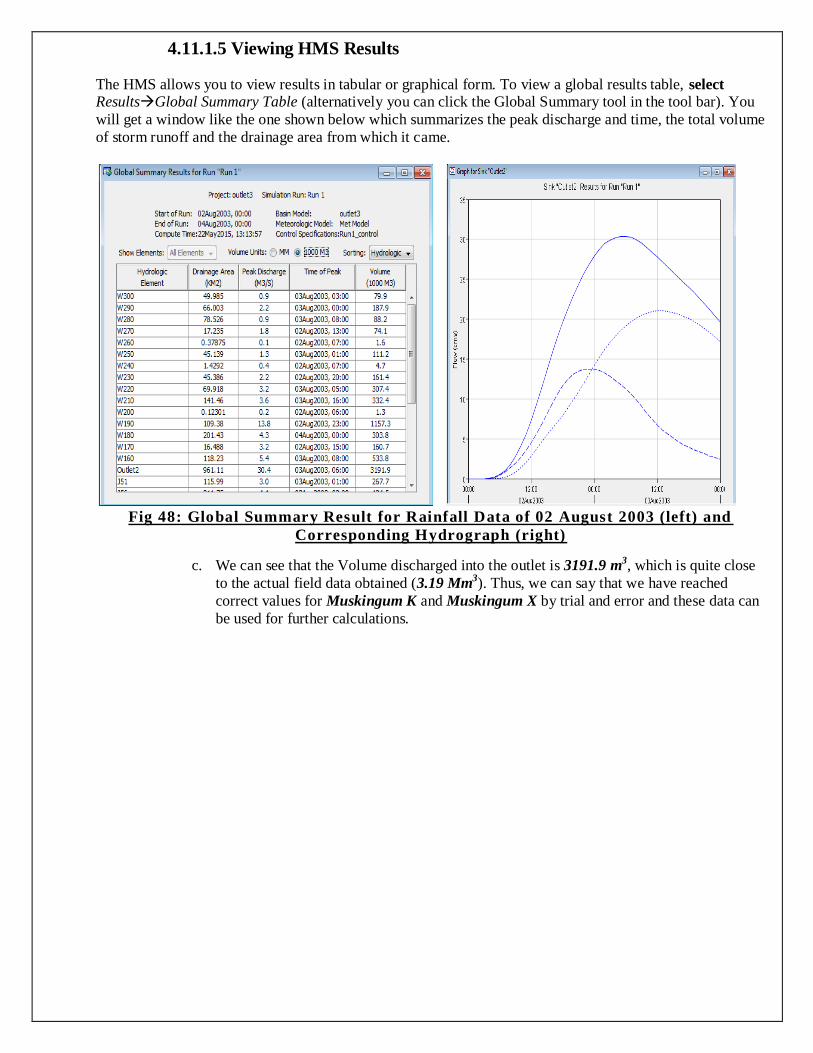
The HMS allows you to view results in tabular or graphical form. To view a global results table, select

ResultsGlobal Summary Table (alternatively you can click the Global Summary tool in the tool bar). You

will get a window like the one shown below which summarizes the peak discharge and time, the total volume

of storm runoff and the drainage area from which it came.

Fig 48: Global Summary Result for Rainfall Data of 02 August 2003 (left) and

Corresponding Hydrograph (right)

c. We can see that the Volume discharged into the outlet is 3191.9 m3, which is quite close

to the actual field data obtained (3.19 Mm3). Thus, we can say that we have reached

correct values for Muskingum K and Muskingum X by trial and error and these data can

be used for further calculations.

5. RESULTS AND CONCLUSION:

The runoff model thus created in the above steps for rainfall on 02nd

August, 2003, needs to be checked

with data of other dates and if correct results are obtained, then we can say that the runoff model created

by us is valid for this catchment.

To check for validity, we do not tamper with the Curve number, Unit Hydrogaph and Muskingum

parameters. We only need to change the values corresponding to the Meteorologic Model and the

Control Specifications.

If running this modified model yields correct results matching the field data, then we can say that the

model is valid; otherwise, this runoff model is not consistent with the given dataset.

We have run this model based on the rainfall data of 10 August 2003, and 13 August 2003. The results

obtained from this run are displayed below:

Fig 49: Global Summary Result for Rainfall Data of 10 August 2003 (left) and

Corresponding Hydrograph (right)

Fig 50: Global Summary Result for Rainfall Data of 02 August 2003 (left) and

Corresponding Hydrograph (right)

From the above Global Summary Results, we can see that the volume corresponding to 10th

August and

13th

August are 1075.6 m3 and 1200.1 m

3 respectively, as opposed to the field data which are 0.09 Mm3

and 2.57 Mm3.

Thus, based on comparison, we can say that the runoff model created by us is not consistent for the

dataset throughout the catchment area considered in our project.

One possible cause of such discrepancy may be due to some problems with the DEM data used. In our

project, we have used DEM data obtained from LISS – III BHUVAN, which had been published on

May 05, 2015. There might be some problems with these DEM data, which have resulted in inconsistent

results. Using the DEM data from more popularly used ASTER data provided by NASA satellites might

lead to correct results using the same procedure. Also, the landuse type of the region, as of 2003 and

2015, are most likely to differ owing to the large scale urbanization and deforestation. Thus, the

classification of land would be altered, which would in turn, affect the CN values of the land area, and

lead to increased runoff as depicted in the model prepared.

Another possible explanation would be improper collection of data at the field. The field data of surface

runoff is not directly available at the site. It is obtained indirectly, using the formula Q = CH1.5. The

discharge is calculated using the available Height of river water at the dam surface, and using Surface

runoff coefficient (C). During this calculation, the typical losses, such as evaporation loss, are not

considered. This gives rise to a significant difference between the calculated runoff and the actual

runoff, as evaporation loss is typically quite high, especially in tropical regions, as in our case.

Thus, we can say, that the model developed by us using the GIS softwares, though inconsistent with the

dataset obtained in the real life scenario, is most likely to provide the actual representation of the surface

runoff at the reservoir.

6. REFERENCE:

1. Chapter 19: classification of Landsat images(supervised) (Remote Sensing in an ArcMap Enviroment

By Tammy Parece; James Campbell; John McGee) http://www.virginiaview.net/education.html

2. Georeferencing in ArcGis10 :

http://resources.arcgis.com/en/help/main/10.1/009t/009t000000mr000000.htm

3. Creating a multi-band GeoTIFF from individual files using ArcGIS 9.3 (RS/GIS Quick Start Guides) :

http://biodiversityinformatics.amnh.org

4. Creating SCS Curve Number Grid using HEC-GeoHMS , Prepared by Venkatesh Merwade ; School

of Civil Engineering, Purdue University

5. Hydrologic Modeling using HEC-HMS : Prepared by Venkatesh Merwade,School of Civil

Engineering, Purdue University

6. HEC-GeoHMS Users Manual 10.1 by US Army Corps of Engineers

7. DEM Data Source : http://bhuvan.nrsc.gov.in/data (published at May 05,2015)

8. Engineering Hydrology by K Subramanya

9. http://en.wikipedia.org/wiki/Runoff_curve_number

10. http://njscdea.ncdea.org/CurveNumbers.pdf

11. https://www.youtube.com/watch?v=uRFm2369INs

12. Enderlin, H. C., and E, M, Markowitz, 1962. The Classification of the soil and vegetative cover

types of California watersheds according to their influences on synthetic hydrographs. Presented at the

Second Western National Meeting of the American Geophysical Union, Stanford University, Palo Alto

California.

13. Price, Myra A. 1998. Seasonal Variation in Runoff Curve Number. MS Thesis, University of

Arizona (Watershed Management). 189pp

14. http://www.water.rutgers.edu/Educational_Programs/CN_gis.htm