Final Report SEP: Wireless Sensors Project Report SEP: Wireless Sensors Project Student: Adam...
78
Final Report SEP: Wireless Sensors Project Student: Adam Lindsay URN 1464795 Academic Supervisor: Dr R Bowden
Transcript of Final Report SEP: Wireless Sensors Project Report SEP: Wireless Sensors Project Student: Adam...

Final Report
SEP: Wireless Sensors Project
Student: Adam Lindsay URN 1464795 Academic Supervisor: Dr R Bowden

SEP: Wireless Sensors Project Final Report
i
Abstract
This report introduces the wireless sensor interface project of the SEP group project.
The objective of the project is to develop a system to collect data from sensors, and to
transmit this data wirelessly to a node which passes the data to a PC. Wireless
transmission methods have been investigated, and it was decided that a proprietary
protocol would be designed. A TDMA based protocol has been designed. Sensor tests
have been performed, and the protocol has been designed and detailed in this report.
This report also discusses the progress made to date on the project, and proposes a
timeline for the completion of the project.

SEP: Wireless Sensors Project Final Report
ii
Acknowledgements
The author would like to thank Robert Owen and the Texas Instruments European
University Team, who donated most of the expensive hardware used in this project.
Without this donation, the project would have been much more limited and difficult.
The author would also like to thank the Freescale and Texas Instruments sample
teams for providing free samples of some of the parts used in the project.
Thanks also go to Dr Bowden for his support as the project's supervisor, and the
members of the SEP team for their teamwork in building a great project.
Finally, the author would like to thank all those who helped by proof reading this
report.

SEP: Wireless Sensors Project Final Report
iii
Contents
1. Introduction 1
1.1 SEP 1 1.2 Wireless sensor interface 1 1.3 Objectives 2 1.4 Specifications 2 1.5 This Report 3
2. Technology Review 4
2.1 Wireless communications 4 2.2 Development platform 12 2.3 Sensors 13 2.4 Power management 15
3. System Overview 18
4. Wireless Protocol 20
4.1 Timing 20 4.2 Packet format 21 4.3 Frequency hopping 22
5. Software 28
5.1 Master 28 5.2 Slave 30 5.3 PC software 32
6. Hardware 41
6.1 Sensors 41 6.2 PC interface 45 6.3 Power management 47 6.4 Hardware design 49
7. Discussions 59
4.1 Project Status 59 4.2 Total Cost 59 4.3 Objectives Achieved 60 4.4 Gannt Chart 61 4.5 Future Work 62
References 63
Appendices
A: Bill of materials 65 B: Pseudo random number generator test results 69 C: Network API Connections 70 D: Algorithm Code Used in SensorDisplay 71

SEP: Wireless Sensors Project Final Report
iv
Table of Figures
1.1 Illustration of wireless sensor system 2 2.1 Fixed assignment TDMA format 4 2.2 Illustration of recovery effect 15 2.3 Discharge characteristics of an AA cell 16 2.4 Discharge characteristics of a DL2/3A cell 16 3.1 Complete system diagram 18 4.1 Wireless transmission timing 20 4.2 Frequency spectrum used by system 26 4.3 Frequency spectrum of two neighbouring channels 27 5.1 Master node block diagram 28 5.2 Master node timing 28 5.3 Slave node block diagram 30 5.4 Slave node timing 30 5.5 Sensorman program flow diagram 33 5.6 SyncAsync program flow diagram 36 5.7 SensorDisplay program flow diagram 38 6.1 Accelerometer test circuit 41 6.2 Logic level converter circuit 42 6.3 Magneto resistor test 1 setup 43 6.4 Magneto resistor test 1 results 43 6.5 Magneto resistor test 2 setup 44 6.6 Magneto resistor test 2 results 44 6.7 RS232 Interface circuit; method 1 45 6.8 RS232 Interface circuit; method 2 46 6.9 DC DC converter test circuit 47 6.10 Discharge characteristics of primary battery types 48 6.11 Mechanical design of system (not to scale) 49 6.12 Main board circuit diagram 50 6.13 Main board PCB design 51 6.14 Main board component placement 51 6.15 RS232/USB board circuit diagram 52 6.16 RS232/USB board PCB design 53 6.17 RS232/USB board component placement 53 6.18 Battery board circuit diagram 54 6.19 Battery board PCB design 54 6.20 Battery board component placement 54 6.21 Master sensor board circuit diagram 55 6.22 Master sensor board PCB design 56 6.23 Master sensor board component placement 56 6.24 Slave sensor board circuit diagram 57 6.25 Slave sensor board PCB design 58 6.26 Slave sensor board component placement 58 7.1 Preliminary Gantt chart 61 7.2 Final Gantt chart 62

SEP: Wireless Sensors Project Final Report
v
Abbreviations
Ack Acknowledgement
ADC Analogue to Digital Converter
AES Advanced Encryption Standard
AI Artificial Intelligence
CRC Cyclic Redundancy Check
CSMA/CA Carrier Sense Multiple Access with Collision Avoidance
CW Contentian Window
DK Development Kit
DoS Denial of Service
EB Evaluation Board
ETSI European Telecommunication Standards Institute
FCC Federal Communications Commission
FHSS Frequency Hopping Spread Spectrum
GPIO General Purpose Input/Output
IFS Inter-Frame Spacing
ISM Industrial Scientific and Medical
LBT Listen Before Talk
MAC Medium Access Control
MCU Microcontroller
NAck Not Acknowledgement
PC Personal Computer
QoS Quality of Service
SEP Special Engineering Project
SMT Surface Mount Terminal
SoC System on Chip
SPI Serial Port Interface
TDMA Time Division Multiple Access
TI Texas Instruments
UAV Unmanned Aerial Vehicle
UGV Unmanned Ground Vehicle
USB Universal Serial Bus
WLAN Wireless Local Area Network

SEP: Wireless Sensors Project Final Report
1
1. Introduction
1.1 SEP
The Special Engineering Project (SEP) is a group final year project with a team
consisting of four members. Each member of the project is developing a system to be
integrated onto a robot.
The SEP was started in 2006, when a team of four created an autonomous robot to
identify and approach a specific object. This robot used a laptop to control the four
motors, and had features such as a wireless positioning system, ultrasound proximity
sensors, and a camera which was used to identify objects.
This year, the team members are:
Ben Abbott AI and project management
Richard Lane UAV control
Adam Lindsay Wireless sensor interface
Affan Shaukat Sound direction sensor
This year, the robot is being improved upon. Ben Abbott has developed the AI system
further, as well as using vision processing to navigate the robot down a corridor.
Richard Lane has added an aerial vehicle, to be autonomously controlled to follow the
robot, and provide an adjustable height camera. Affan Shaukat has developed a sensor
to locate the direction of a sound source. The author has developed a system for
wirelessly connecting sensors to the robot. The vehicles are being developed with an
autonomous surveillance application in mind, for example, a security system.
1.2 Wireless sensor interface
This report is concerned with the wireless sensor interface project. The aim of the
wireless interface project is to develop a system to collect data from sensors, and to
transmit this data wirelessly to a node which passes the data to a PC mounted on the
UGV, where the data can be used by the robot's AI. The system is to be designed with
expandability and flexibility in mind. i.e. the system should allow for further sensors
and nodes to be added. The system is illustrated in fig 1.1.

SEP: Wireless Sensors Project Final Report
2
Fig 1.1 Illustration of wireless sensor system
1.3 Objectives
Primary:
-Create a wireless data transmission system
-Collect sensor data
-Communicate data to the PC
Secondary:
-Implement a frequency scan
-Implement frequency hopping
-Provide an estimation of distance between nodes
-Implement a battery level monitor
1.4 Specifications
The system is required to operate with the following specifications:
1. Sensor readings must be taken at 50Hz (minimum)
2. The sensor readings must be communicated to the PC in the correct order, with
minimal delay. This means a maximum delay of 20ms.
3. The system must communicate the sensor readings to the PC via USB
4. The system must not interfere with the robots other systems
5. The wireless node must be lightweight, since it has to be attached to a UAV
PC
Sensor
Sensor
Sensor
Sensor
Sensor
Sensor
Transmitter
Transmitter
Receiver Buffer /
MCU
Sensor Sensor
USB link
Wireless
link
Possible
expansion
UAV UGV

SEP: Wireless Sensors Project Final Report
3
1.5 This Report
This report will begin by presenting a review of technologies investigated for use in
this project. This review discusses possible approaches for different elements of the
project, and also looks into some of the theory which is used by the different
approaches. It also contains some information about the hardware being used in the
project. Next, a brief overview of the system is given so that the reader can appreciate
how each of the different elements of the system fit together. After this, the wireless
protocol design is given. This is discussed first, because this is the backbone of the
system, with the operation of the rest of the system being designed around this. Next,
software elements of the project are given. This allows the reader to see the flow of
data, from the slave to the PC programs which use it. Chapter 6 will provide
information about the hardware used, experiments carried out, and specific details of
the design and implementation of the project. The design of the final system is given
in this section. The report will conclude in chapter 7 by discussing the success of the
project. The report will end by discussing the progress against the projected timeline
of the project, and discussing how the project could progress.
SEP: Wireless Sensors Project Final Report
4
2. Technology Review
2.1 Wireless Communications
2.1.1 Multiple Access Techniques
If there is more than one node to transmit, then there needs to be a method by which
the multiple nodes do not interfere with each other. This section will discuss a few of
these techniques.
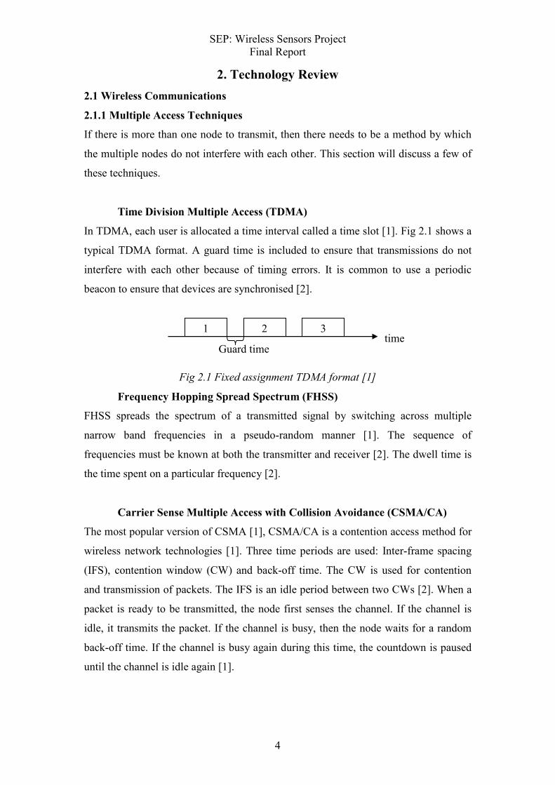
Time Division Multiple Access (TDMA)
In TDMA, each user is allocated a time interval called a time slot [1]. Fig 2.1 shows a
typical TDMA format. A guard time is included to ensure that transmissions do not
interfere with each other because of timing errors. It is common to use a periodic
beacon to ensure that devices are synchronised [2].
Fig 2.1 Fixed assignment TDMA format [1]
Frequency Hopping Spread Spectrum (FHSS)
FHSS spreads the spectrum of a transmitted signal by switching across multiple
narrow band frequencies in a pseudo-random manner [1]. The sequence of
frequencies must be known at both the transmitter and receiver [2]. The dwell time is
the time spent on a particular frequency [2].
Carrier Sense Multiple Access with Collision Avoidance (CSMA/CA)
The most popular version of CSMA [1], CSMA/CA is a contention access method for
wireless network technologies [1]. Three time periods are used: Inter-frame spacing
(IFS), contention window (CW) and back-off time. The CW is used for contention
and transmission of packets. The IFS is an idle period between two CWs [2]. When a
packet is ready to be transmitted, the node first senses the channel. If the channel is
idle, it transmits the packet. If the channel is busy, then the node waits for a random
back-off time. If the channel is busy again during this time, the countdown is paused
until the channel is idle again [1].
1 2 3 time
Guard time
SEP: Wireless Sensors Project Final Report
5
2.1.2 Network Security
There are many types of attack which can be used on a wireless network. Here we
will look at relevant methods of attack, and how they can be overcome.
Types of attack
DoS: Denial of Service
A DoS attack prevents access to a service or resource. There are two general forms of
DoS attack: those that crash services, and those that flood services [3]. DoS attacks
that crash services are often dependant on poor implementation, e.g. causing buffer
overflows [3]. In wireless networking, a common approach is to jam the frequency
being used. FHSS is a common technique used to overcome jamming attacks [2].
Sniffing
The act of capturing packets that aren't necessarily for public viewing is called
sniffing [3]. Using a powerful encryption will stop a sniffing device from being able
to read the packet [2].
Impersonation
In an impersonation attack, the malicious node assumes the identity of an authorised
node. This could be done by correctly guessing the identity of the node, or by
snooping for the identity of the node. In the scope of this report, this type of attack
might use the malicious node to pass false information to the master node. [2]
Cryptology
Encryption can be used to avoid packet sniffing [2]. Here, Symmetric and
Asymmetric encryption will be explained.
Symmetric Encryption
Symmetric encryption is a cryptosystem where the same key is used to both encrypt
and decrypt the message. It generally requires less computation than asymmetric
encryption, but it can be difficult to distribute the key [3].
Asymmetric Encryption
An asymmetric cryptosystem uses 2 keys: a public key and a private key. Data is
encrypted using the public key, but can only be decrypted using the private key. This
eliminates the problem of key distribution [3], but can require more computational
resources [3].

SEP: Wireless Sensors Project Final Report
6
2.1.3 Wireless Networking Protocols
There are several wireless networking standards defined, and others still being
finalized. This section will look at several protocols, and discuss the advantages and
disadvantages of each protocol. These will then be compared to a proprietary protocol.
Bluetooth
Bluetooth is an open specification for short range voice and data communications [1].
It operates in the 2.4GHz ISM band [1]. Bluetooth uses a frequency hopping sequence
based on the master clock and master address [2]. Devices are authenticated using a
challenge-response mechanism based on a user defined PIN. It is also possible to
encrypt the link [2]. Power consumption can be up to 100mW. It has a typical range
of less than 10m and a peak data rate of 1Mbps is available [2]. Bluetooth uses
timeslots of 625µs [2]. The master may only begin a transmission on an even timeslot,
and slaves may only begin transmission in an odd timeslot. A slave may only transmit
(normally) if it received a packet from the master in the previous timeslot [2]. This
means a maximum of 16 slaves to meet the specifications (Using the equation in
appendix.A).
Advantages:
-Frequency hopping provides resilience to DoS attacks
-An Ack/NAck is used to confirm successful data transmission [2]
-No transmission contention delays
Disadvantages:
-Bluetooth devices must remain in an active state for the entire time they are
connected to the network [2]
ZigBee
The ZigBee protocol is designed for use in wireless sensor networks. ZigBee uses the
2.4 GHz frequency band for higher bandwidth and world-wide acceptance along with
the ETSI 868 MHz and the FCC 900 MHz bands [6]. ZigBee uses a CSMA/CA
transmission system, based on the IEEE 802.15.4 MAC layer [6]. The MAC layer
provides AES encryption. ZigBee devices have been proven to communicate
effectively in environments with significant interference [7]. ZigBee supports a data
rate of 250kbps.

SEP: Wireless Sensors Project Final Report
7
Advantages:
-Standard based security protocol
-Designed for low power applications
-Mesh network means better range when many nodes are involved
Disadvantages:
-Complex (relative to required system)
-Transmission contention (CSMA/CA) means no guarantee of how long a
transmission can take
-Low data rate
IEEE 802.11b (WLAN) and TCP
802.11b can achieve data rates of 11Mbps, using the 2.4GHz frequency band [2]. It is
widely used in PC networking. 802.11b uses timeslots of 20µs [2], and a CSMA/CA
transmission scheme [2]. Between each transmission, a back-off time must take place.
This time is frozen whilst the transmission medium is busy [2]. This back off time is a
random value between 31 and 1023 time slots (640µs and 20460µs) [2].
Advantages:
-High data rate
-Priority possible for delay-sensitive packets [2]
Disadvantages:
-High current consumption (in the order of 100mA) [2]
-Possibility of long delays before receiving data due to back-off and contention
-Possible contention issues with PC WLAN
Designing a Proprietary Protocol
It is possible to design a proprietary protocol, specifically for the application in this
report. This would trade off some of the system's flexibility for performance. A time-
slotted approach could be used to eliminate contention, so that transmission delay is
invariant. Frequency hopping can be used to reduce the risk of DoS attacks (as well as
improving tolerance to interference), and predefined network structure can be used to
eliminate authentication-based attacks. A pre-defined structure, along with time-slot
allocation would also allow for a low-power system since much unnecessary overhead
can be eliminated. It is possible to use encryption, using a pre-shared key, to reduce
the risk of packet sniffing. It is also possible to ensure QoS using a redundancy check.

SEP: Wireless Sensors Project Final Report
8
The main disadvantage to designing a proprietary protocol is the effort required. It
will also leave the system incompatible with other systems.
Advantages:
-Lower power achievable
-Secure system achievable
-Consistent delay in data reception
-Possible interference resilience
Disadvantages:
-Greater effort required to design proprietary protocol
-Incompatibility with other systems
Summary
Due to the restrictions on the delay for the data to arrive, contention-based protocols
(ZigBee [6], IEEE 802.15.4 [2]) fail to offer guaranteed transmission within the time
restriction of 20ms (50Hz). Bluetooth can meet the time limitation and all other
specifications. Because the power consumption of the slaves is relatively high (around
100mW [2]), this would mean a (relatively) large battery would be required. This is
undesirable, since it adds size and weight to the solution. A proprietary protocol can
be designed to meet the specifications. This will make the device incompatible with
other systems. However, since the system needs to be secure, this may prove to be an
advantage. The main disadvantage of using a proprietary protocol is the effort
required in designing it. However, it is the author's opinion that the effort of designing
a protocol will be outweighed by the advantages of using such a protocol.
2.1.4 Radio Frequency Regulations
There are two frequency bands which are free to use for Industrial, Scientific and
Medical applications. These bands are at 868MHz, and 2.4GHz. Each band has
different regulations, which are defined by the European Telecommunications
Standards Institute (ETSI). This section will describe the applicable regulations, then
the advantages of each band will be compared.
SEP: Wireless Sensors Project Final Report
9
868MHz Regulations
The 868MHz band discussed here is between 868MHz and 868.6MHz. For a 14dBm
(25mW) output power, a 1% duty cycle or LBT must be used [4]. There are no limits
on the channel spacing. There are no additional benefits for using FHSS.
2.4GHz Regulations
The 2.4GHz band between 2400MHz and 2483.5MHz is available for generic use [5].
This band has no duty cycle restrictions [5]. LBT is not required [5]. The output
power is restricted to 10mW (-20dBm) for non spread spectrum uses [5]. If FHSS is
used, then an output power of 100mW (-10dBm) is allowed [5]. For non-adaptive
FHSS, the system must "…make use of at least 15 well defined, non-overlapping
hopping channels separated by the channel bandwidth as measured at 20 dB below
peak power… the minimum channel separation shall be 1 MHz, while the dwell time
per channel shall not exceed 0,4 s… each channel of the hopping sequence shall be
occupied at least once during a period not exceeding four times the product of the
dwell time per hop and the number of channels." [5] This gives a maximum of 83
channels.
Summary
868MHz advantages:
-Longer range for same output power. (Due to physical laws) [1]
2.4GHz advantages:
-More channels are available.
-Higher output power available for FHSS systems
-Smaller antenna used. (Due to physical laws)
-No duty cycle or LBT limitations

SEP: Wireless Sensors Project Final Report
10
2.1.5 Pseudo Random Number Generation
If a frequency hopping system is to be used, then a method of generating apparently
random numbers is required. Since the numbers must be generated at both the
transmitter and receiver, using an algorithm to generate these numbers will ensure the
same nubers are generated at each end.
James E Gentle states that two basic techniques for generating pseudo random
sequences are commonly used: congruential methods and feedback shift register
methods. This report only looks at congruential methods [13]. This basic relationship
can be written in the form:
mba mod≡
Lagged Fibonacci Generator
The lagged Fibonacci generator is a simple recursive generator of the form [13]:
mxxx kijii mod)( −− +≡
If m, j and k are chosen properly, then a large period can be achieved.
It has been shown that care must be taken when choosing the initial values for a
lagged Fibonacci generator, but for a well selected initial sequence, a better apparent
randomness than non-recursive generators can be achieved.
Nonlinear Congruential Generators
A generalisation of the congruential generator has been proposed [13]:
mcaxdxx iii mod)( 1
2
1 ++≡ −−
Such a generator has the disadvantage that more computations are required. However,
using polynomials has the apparent advantage of making the generator less obvious.
Combined Generators
It is suggested that a combination of two generators may improve the apparent
randomness properties. Conversely, however, it is also possible that the undesirable
properties of the two generators could be magnified, creating a worse generator.
Although using combined generators may make the sequence more difficult to predict,
it may also affect the uniformity of the generator [13], causing certain numbers to be
favoured over others.

SEP: Wireless Sensors Project Final Report
11
Quality of Random Number Generators
Lack of fit
James E. Gentle proposes that "The quality of a random number generator depends
on how closely the properties of the output of the generator match the properties of an
independent and stationary uniform data generating process. To assess quality, we
need quantitative measures of differences of the properties of the output stream and
an ideal stream…"[13]. Since this report is only concerned with uniform generators, a
measure of deviation from a uniform distribution can be used.
Independence
The apparent mutual independence of the values in the output stream is also of
importance. One way to measure independence is to compute the correlation between
values at fixed lags [13]. Computing the correlation can help to highlight a repetitive
stream, or sub-stream within the output of the generator.

SEP: Wireless Sensors Project Final Report
12
2.2 Development Platform
After contacting Texas Instruments (TI), the university has been offered a donation of
the necessary development hardware and software for the wireless sensors project.
Therefore, some products from Texas Instruments have been compared. There are 2
combinations of products from TI which could be used; a radio, with a MCU on-chip
(SoC) or a separate radio and MCU. The advantages and disadvantages of each are
given here.
SoC:
Advantages:
-USB-ready radio chip, CC2511 available. [8]
-No need to interface external MCU.
-Less space required
Disadvantages:
-Expensive compiler software required (IAR software) [8]
-Few ADC channels
Separate devices:
Advantages:
-Free compiler software
-Many on-chip interfaces available [9]
Disadvantages:
-More space required
-Separate USB interface required
The IAR compiler was found to cost in the region of ₤500, therefore the decision was
made to use separate devices. It was desired to use the MSP430 Experimenters board
[9]; a development board which allows a Chipcon EB to be easily interfaced.
However, these boards were not available until early December because of lack of
stock.
Therefore, the following hardware was donated by TI:
1 of CC2500-2550 DK [8]
2 of MSP-FET430U100 and MSP430FG4618 [9]
1 of Code Composer Essentials [9]

SEP: Wireless Sensors Project Final Report
13
2.3 Sensors
Several different types of sensor, which are applicable to an autonomous vehicle, are
available. This section splits the sensors into 2 groups: pre-built sensor modules and
independent sensors. Both groups have been evaluated.
2.3.1 Sensor modules
Four orientation/acceleration modules from three companies were investigated. The
features of the products are shown in table 2.1. The modules use RS232 or USB.
Company Part Price Sensors
Microstrain 3DM-DH $895 Orientation: Pitch ±90˚ roll ±180˚ yaw ±180˚
3DM-GX1 $1500 Orientation: 360˚ in all axes.
X-Sens MTi $2550 Rate of turn, acceleration and magnetic field
in 3 axes.
Motion Node $1000 Rate of turn, acceleration and magnetic field
in 3 axes. Orientation calculated.
Table 2.1 – Complete sensor module solutions comparison
Although these sensors would be ideal for use with the UAV, they are too expensive
for use in the system.
2.3.2 Independent Sensors
Many independent sensor chips are available. These sensors normally measure one
specific effect (e.g. acceleration) along one or more axes. For each effect to be
measured, this subsection discusses some solutions available.
Acceleration
Freescale, a semiconductor company, produce 3-axis accelerometers with analogue
outputs (single ended) for each axis. The MMA7260QT allows for a selection of
acceleration sensitivities, and also offers a sleep mode (for low power applications).
Samples of the MMA7260QT can be obtained free of charge using Freescale's sample
ordering system.
Rate of turn (gyroscope)
A 2-axes chip gyroscope is available from Invensense. This part is cheaper than many
competitors single axis chip gyroscopes. The IDG-300 outputs a single ended
analogue signal for each axis. This part can be obtained for under ₤50.

SEP: Wireless Sensors Project Final Report
14
Odometer (wheel encoder)
Active-Robots, a robotics parts company, sell a pair of wheel encoder disks and
sensors for under ₤30. The disk has 44 spokes, allowing for a resolution of 8.2˚.
Magneto resistor
A magneto resistor measures the strength of a magnetic field. This can be used to
provide a digital compass. NXP offer a single axis magneto resistor with a differential
analogue output. Honeywell produces 2-axis magneto resistors, also with a
differential analogue output. The HMC1002 from Honeywell is stated as being able to
measure the Earth's magnetic field. This part is available for around ₤15.

SEP: Wireless Sensors Project Final Report
15
2.4 Power Management
2.4.1 Low Power Techniques
Energy management is an important issue in sensor networks. Efficient battery
management, transmission power management and system power management are the
three major means of increasing the life of a node [2].
Battery Management
The system should try to maximize the amount of energy provided by the battery by
exploiting the physical properties of the battery [2]. An effect which can be easily
exploited is the 'recovery capacity effect'. This effect is concerned with the recovery
of charge when the system is idle, as shown in fig 2.2. By increasing the idle time of
the system, it can be possible to use the theoretical capacity of a cell [2].
Fig 2.2 Illustration of recovery effect [2]
2.4.2 Battery Technologies
There are many different battery types available, with different sizes, weights,
capacities and voltages. This section will look at a few of the standard, non-
rechargeable types of battery and then discuss the advantages and disadvantages of
each.
Alkaline Manganese
This battery type includes the standard sizes, such as AA used in many digital
cameras and personal stereos / MP3 players. These batteries come in a range of sizes,
and are generally quite large. They do, however, tend to have a large capacity. Fig 2.3
shows the discharge characteristic of an AA cell (taken from Duracell [12]). It can be
seen that the voltage can vary greatly over the operating life of the battery.
Discharge Recovery effect
Time
Vo
ltag
e
Time
Cu
rren
t
On Idle

SEP: Wireless Sensors Project Final Report
16
Fig 2.3 Discharge characteristic of an AA cell [12]
An AA battery (MN1500) will operate for around 200 hours, if a 10mA load is
attached.. A standard AA cell is 23.8g in weight, and 50.5mm long, with a diameter of
14.5mm.
Lithium Manganese
These are high capacity batteries, often used in photography applications. They are
characterised by their flat discharge characteristic, shown in fig 2.4. A DL123A cell
would provide between 3V and 2V for 130 hours with a 10mA load connected.
Fig 2.4 Discharge characteristic of an DL2/3A cell [12]
A DL123A cell is 34.5mm high and 17.0mm in diameter, weighing 17g.

SEP: Wireless Sensors Project Final Report
17
Zinc Air
Zinc Air batteries are often used for medical, communications, and monitoring
applications, including hearing aids. The 675 cell has a nominal voltage of 1.4V. IT
has a flat discharge characteristic, and will last 55 hours connected to a 10mA load. It
is 11.6mm in diameter, and 5.4mm high. One cell weighs 1.8g. It should be noted that
this cell is susceptible to oxygen starvation if used in a sealed environment.
Silver Oxide
The silver oxide battery is used in applications such as low-power LCD watch and
calculator displays. Silver Oxide batteries are stated as having a flat, stable discharge
characteristic [12]. The MS76 cell, which has a nominal voltage of 1.55V, will last
approximately 18 hours with a 10mA load connected. The cell has a diameter of
11.6mm, and a height of 5.4mm. One cell weighs 2.3g.
Summary
• The standard Alkaline Manganese batteries have a large capacity, however they are
large, heavy, and the output voltage varies greatly over the life of the battery.
• Lithium manganese batteries have a larger capacity, and a flat discharge
characteristic, however they are still relatively large and heavy.
• Zinc Air batteries are relatively small and lightweight. However, they do not have a
large capacity, and are susceptible to oxygen starvation if incorrectly installed.
• Silver oxide batteries are extremely small and lightweight. However, they have a
very small capacity.
It was decided that zinc air batteries will be used for the project, since they have an
acceptable capacity, and are very lightweight and small. The size and weight are the
most important criteria, since the device will need to be attached to the UAV.

SEP: Wireless Sensors Project Final Report
18
3. System Overview
A block diagram of the overall system which has been designed is shown in fig 3.1.
fig 3.1 complete system diagram
Sensorman
Gyroscope
Radio
Odometer
Accelerometer
Wireless
Link
RS232 to
USB
MCU
Compass
Accelerometer
Compass
Tilt switches
Radio
LED
Power Mgmt.
MCU
Power Mgmt.
Slave
Master
UA
V
UG
V
PC
Virtual COM port
SensorDisplay / SyncAsync / AI
USB
LED

SEP: Wireless Sensors Project Final Report
19
The node attached to the UAV will have a number of sensors built into it. These
sensor readings will be collected by the MCU and sent to the master node (on the
UGV) by a proprietary wireless protocol on the 2.4 GHz spectrum.
The master node collects receives the sensor readings, and also takes sensor readings
from sensors attached to the UGV. These sensor readings are then transmitted to the
PC over USB by using a RS232 to USB converter to create a virtual COM port on the
PC.
The PC should be running a program, which has been developed to receive the sensor
readings, and forward them on to another process using the Network API developed
by Ahmed Aichii in 2006/7.
In the following sections, firstly the wireless protocol will be discussed. The wireless
protocol is the backbone of the system, and all other systems have been developed
around this. Next, the software elements of the system will be discussed. Finally, the
hardware development and final designs are given.
SEP: Wireless Sensors Project Final Report
20
4. Wireless Protocol
The protocol has been designed as a star network, using a TDMA approach. The
master will transmit a beacon frame, which may also contain communications to a
specific node. Once this beacon frame has been received by a slave, the slave will
wait a fixed period of time before transmitting its data to the master. There are 6
available time slots for the slave to transmit in. The nodes will be pre-programmed
with the device address and slot allocation. This will avoid overhead due to
authentication and commissioning.
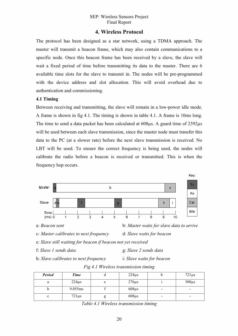
4.1 Timing
Between receiving and transmitting, the slave will remain in a low-power idle mode.
A frame is shown in fig 4.1. The timing is shown in table 4.1. A frame is 10ms long.
The time to send a data packet has been calculated at 608µs. A guard time of 2392µs
will be used between each slave transmission, since the master node must transfer this
data to the PC (at a slower rate) before the next slave transmission is received. No
LBT will be used. To ensure the correct frequency is being used, the nodes will
calibrate the radio before a beacon is received or transmitted. This is when the
frequency hop occurs.
a: Beacon sent b: Master waits for slave data to arrive
c: Master calibrates to next frequency d: Slave waits for beacon
e: Slave still waiting for beacon if beacon not yet received
f: Slave 1 sends data g: Slave 2 sends data
h: Slave calibrates to next frequency i: Slave waits for beacon
Fig 4.1 Wireless transmission timing
Period Time d 224µs h 721µs
a 224µs e 276µs i 500µs
b 9.055ms f 608µs - -
c 721µs g 608µs - -
Table 4.1 Wireless transmission timing

SEP: Wireless Sensors Project Final Report
21
If a beacon is not received by a slave, it will extend the Rx time by 0.5ms (250µs
extra before and after previous Rx time). If a beacon is then received, the Rx time will
return to normal. If 4 consecutive beacons are not received, the device will device will
return to the starting frequency and remain in Rx mode until a beacon is received.
4.2 Packet Format
A slave data packet will be in the format shown in table 4.2. Reserved bits must be set
to 0. They will be ignored at the receiving end.
Section Length (bits) *Header Length
Preamble 16 Slave Address 8
Sync word 32 Battery Remaining 3
Packet Length 8 Reserved 5
Dest. Address 8 ** Port 1..13 Length
Header* 16 Reserved 3
Port 1 .. 13** 16 per port GPIO state 1
CRC 16 Sensor Value 12
Table 4.2 Slave packet format
The beacon is in the format shown in table 4.2. The beacon identifier is 0xBC for this
system. All unrecognised commands will be discarded by the slave device.
Section Length (bits) Command* Byte1 Byte2
Preamble 16 No Command 0x00 0x00
Sync word 32 Set GPIO port high 0x01 Port #
Packet Length 8 Set GPIO port low 0x02 Port #
Dest. Address 8
Beacon Ident. 8
Command Addr 8
Command* 16
CRC 16
Table 4.3 Master Packet Format

SEP: Wireless Sensors Project Final Report
22
4.3 Frequency Hopping
In order to be able to use a higher transmission power, the ETSI standard requires
frequency hopping to be used. To create a frequency hopping system, both the
transmitter and receiver must know what frequency will be used at any time. To
implement channel hopping, a pseudo random number generating algorithm will be
used. This algorithm will generate a series of apparently random numbers, between
zero and the maximum channel number.
4.3.1 Requirements
The ETSI standards state that the system should "…make use of at least 15 well
defined, non-overlapping hopping channels separated by the channel bandwidth as
measured at 20 dB below peak power… the minimum channel separation shall be 1
MHz,".[4] The channel bandwidth was measured to be approximately 1.8MHz. The
ETSI standards also state that no spurious emissions above -30dBm should be
measured outside the 2.4-2.483.5 GHz bandwidth. Therefore, channels should occur
between 2.402 GHz and 2.480 GHz (inclusive) to ensure this criterion is met. With a
channel spacing of 2MHz, this allows for 40 channels.
Channel 40 is used as a start channel. This channel shall only be visited once, at the
start of the sequence. This will allow the master and slave devices to synchronize.
Channels 1 to 39 are used pseudo randomly.
Because "… each channel of the hopping sequence shall be occupied at least once
during a period not exceeding four times the product of the dwell time per hop and the
number of channels." [4] the maximum length of the sequence is 1600ms, or 160 hops
if one hop occurs every time a beacon is sent. A sequence 150 long is used, to ensure
this criterion is met.
SEP: Wireless Sensors Project Final Report
23
4.3.2 Algorithm
The algorithm must meet a number of criteria:
- It must have an approximately uniform distribution over the range of channels.
- It must be non-repetitive for the length of the sequence.
The implementation requires a number of other constraints:
- The number of channels must be 39.
- At any point in the calculation, no number may exceed 2^15.
- At any point in the calculation, all numbers must remain natural positive.
- The sequence shall be 150 values long.
- There should be 32 possible selectable sequences generated by the algorithm.
The last point was decided so that different sequences can be selected by the user on
startup.
Algorithm 1
The following algorithm, suggested in [13], was investigated:
For
++≡≥
++≡<∈++
−−
−−−−
mbaxxxm
mcaxxxmcaxx
nnn
nnnnn
mod)(:
mod)(:)(
1
2
1
1
2
11
2
1
Where m is the number of channels to be used, and a, b and c are integer values.
The algorithm was tested using excel, using various small integer values for A, B, C
and seeds. However for the relatively small values of m being used (<100), the
algorithm was found to often fall into a repetitive pattern.
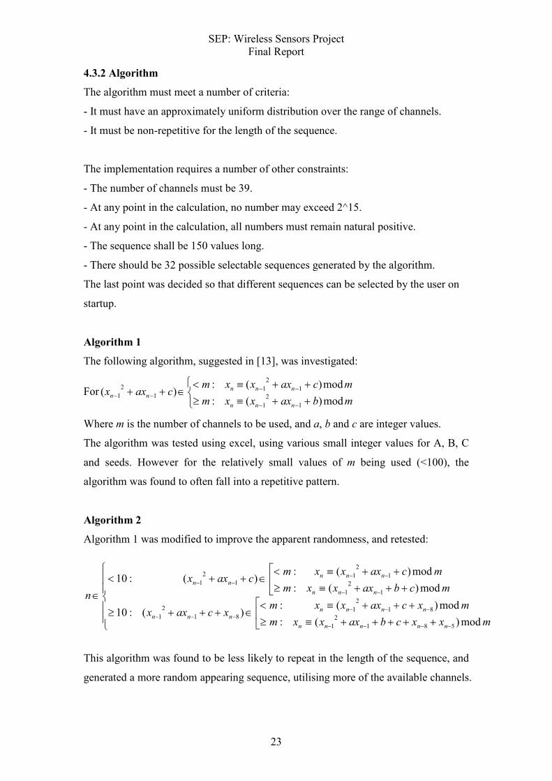
Algorithm 2
Algorithm 1 was modified to improve the apparent randomness, and retested:
This algorithm was found to be less likely to repeat in the length of the sequence, and
generated a more random appearing sequence, utilising more of the available channels.
+++++≡≥
+++≡<∈+++≥
+++≡≥
++≡<∈++<
∈
−−−−
−−−−−−
−−
−−−−
mxxcbaxxxm
mxcaxxxmxcaxx
mcbaxxxm
mcaxxxmcaxx
n
nnnnn
nnnnnnn
nnn
nnnnn
mod)(:
mod)(:)(:10
mod)(:
mod)(:)(:10
581
2
1
81
2
181
2
1
1
2
1
1
2
11
2
1
SEP: Wireless Sensors Project Final Report
24
Selecting a, b, c and seed values
Algorithm2 was tested using Microsoft Excel. 32 sequences of 150 numbers were
generated, with m = 39.
The sequence to be generated was set by 5 bits.
Bits 0 and 1 select between 4 possible seed values.
Bit 2 selects between 2 possible values of a.
Bit 3 selects between 2 possible values of b.
Bit 4 selects between 2 possible values of c.
Possible values of a b and c were generated using some standard integer sequences.
Seeds were assumed to be either 0-3 or 1-4. From this, all 32 sequences were
generated, and a sum of the number of times each channel occurs was made. From
this, the standard deviation of the occurrence of each channel was calculated. A low
standard deviation signals that each channel is used equally. A high standard
deviation signals that some channels are favoured. The complete set of results are
given in Appendix B.
For the values with the 10 lowest standard deviations, the covariance of each value in
a sequence was calculated. The average of the absolute value of this was taken from
all 32 sequences. If there is no discernable pattern, this number will be high. If there is
a pattern is the sequence, this number will be low. The percentage of number of
channels visited at least once by a sequence was calculated for each of the 32
sequences and averaged. The minimum channel usage was also calculated. It is
desirable for the minimum channel usage to be as high as possible, since this means
that there will be no channel which doesn't visit most of the available spectrum. It also
helps to highlight whether one of the sequences follows a pattern, or rejects certain
channels. The results are shown in table 4.4. The best results are highlighted.

SEP: Wireless Sensors Project Final Report
25
1a 2a 1b 2b 1c 2c seed σ Avg xa Avg chan use (%) Min chan use (%)
2 3 11 13 5 7 1-4 5.73 10.089 97.8 92.3
5 7 2 3 11 13 1-4 6.01 10.662 97.3 87.2
5 7 11 13 2 3 1-4 5.68 10.582 97.6 92.3
2 3 13 17 5 7 1-4 5.86 10.196 98.0 92.3
5 7 2 3 13 17 1-4 5.83 10.596 96.2 66.7
5 7 13 17 2 3 1-4 5.99 10.822 97.4 92.3
3 4 1 2 5 7 1-4 6.06 9.804 97.6 92.3
3 4 5 7 1 2 0-3 5.69 10.328 98.3 94.9
3 4 5 7 1 2 1-4 5.60 10.046 97.8 94.9
5 7 1 2 3 4 1-4 6.09 10.145 96.6 66.7
Table 4.4 test results
From these results, it is clear that using the values of:
1a = 2, 2a = 2, 1b = 5, 2b = 7, 1c = 1, 2c = 2, seed = 0-3.
will generate the best set of sequences from the values tested.
SEP: Wireless Sensors Project Final Report
26
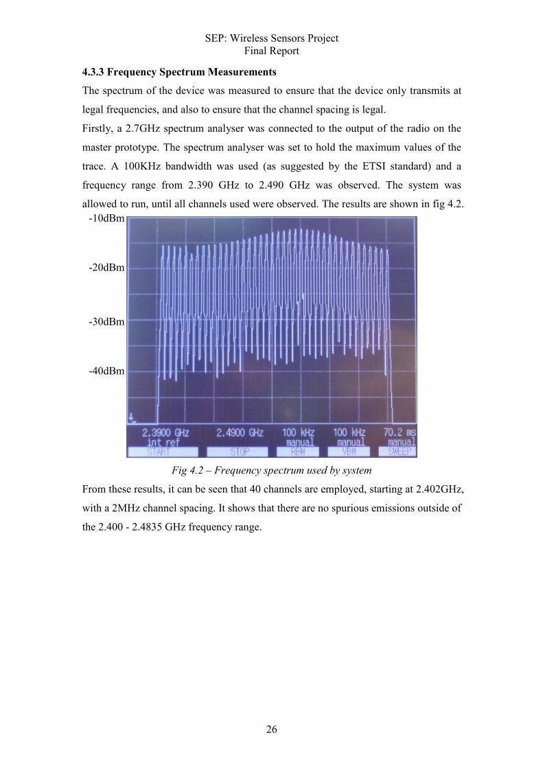
4.3.3 Frequency Spectrum Measurements
The spectrum of the device was measured to ensure that the device only transmits at
legal frequencies, and also to ensure that the channel spacing is legal.
Firstly, a 2.7GHz spectrum analyser was connected to the output of the radio on the
master prototype. The spectrum analyser was set to hold the maximum values of the
trace. A 100KHz bandwidth was used (as suggested by the ETSI standard) and a
frequency range from 2.390 GHz to 2.490 GHz was observed. The system was
allowed to run, until all channels used were observed. The results are shown in fig 4.2.
Fig 4.2 – Frequency spectrum used by system
From these results, it can be seen that 40 channels are employed, starting at 2.402GHz,
with a 2MHz channel spacing. It shows that there are no spurious emissions outside of
the 2.400 - 2.4835 GHz frequency range.
-10dBm
-20dBm
-30dBm
-40dBm

SEP: Wireless Sensors Project Final Report
27
Next, the frequency range of the spectrum analyser was set to 2.443 – 2.447 GHz. The
test was repeated, and the results are shown in fig 4.3.
Fig 4.3– Frequency spectrum of two neighbouring channels
These results show that the system has a channel spacing of 2MHz. The channels are
non-overlapping, as they are below -20dB of the peak power halfway between the
channels. It can also be seen that the peak output power is below the -10dBm limit.
From these measurements, it can be seen that the system meets the requirements set
by the ETSI standard.
-10dBm
-20dBm
-30dBm
-40dBm

SEP: Wireless Sensors Project Final Report
28
5. Software
5.1 Master
A block diagram of the master node is shown in fig 5.1.
Fig 5.1 Master node block diagram
The master node is programmed to collect ADC conversions and counter counts, and
then transmits these to a PC. The master also sends a beacon packet periodically, and
receives sensor data from slaves. This data is sent to the PC as it is received.
The program flow is shown in pseudo code over the page. Interrupts are shown in
order of normal occurrence. The timing of each interrupt, and the time spent outside
of idle mode is shown in fig 5.2. Interrupt 4 can occur at any time.
a: Beacon sent b: Master waits for slave data to arrive
c: Master calibrates to next frequency d: Master sends sensor data to PC
e: Slave data arrives f: Master sends slave data to PC
Fig 5.2 Master node timing
Counter
Accelerometer
Magneto
resister
Odometer
Odometer
LPF
LPF
LPF
Level shift
Level shift
ADC
MSP430FG4619
CC2500
SPI
USB
Interface
RS
232
GPIO LED
SEP: Wireless Sensors Project Final Report
29
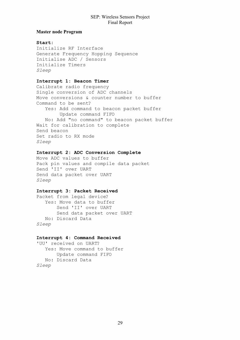
Master node Program
Start:
Initialize RF Interface
Generate Frequency Hopping Sequence
Initialise ADC / Sensors
Initialize Timers
Sleep
Interrupt 1: Beacon Timer
Calibrate radio frequency
Single conversion of ADC channels
Move conversions & counter number to buffer
Command to be sent?
Yes: Add command to beacon packet buffer
Update command FIFO
No: Add "no command" to beacon packet buffer
Wait for calibration to complete
Send beacon
Set radio to RX mode
Sleep
Interrupt 2: ADC Conversion Complete
Move ADC values to buffer
Pack pin values and compile data packet
Send 'II' over UART
Send data packet over UART
Sleep
Interrupt 3: Packet Received
Packet from legal device?
Yes: Move data to buffer
Send 'II' over UART
Send data packet over UART
No: Discard Data
Sleep
Interrupt 4: Command Received
'UU' received on UART?
Yes: Move command to buffer
Update command FIFO
No: Discard Data
Sleep
SEP: Wireless Sensors Project Final Report
30
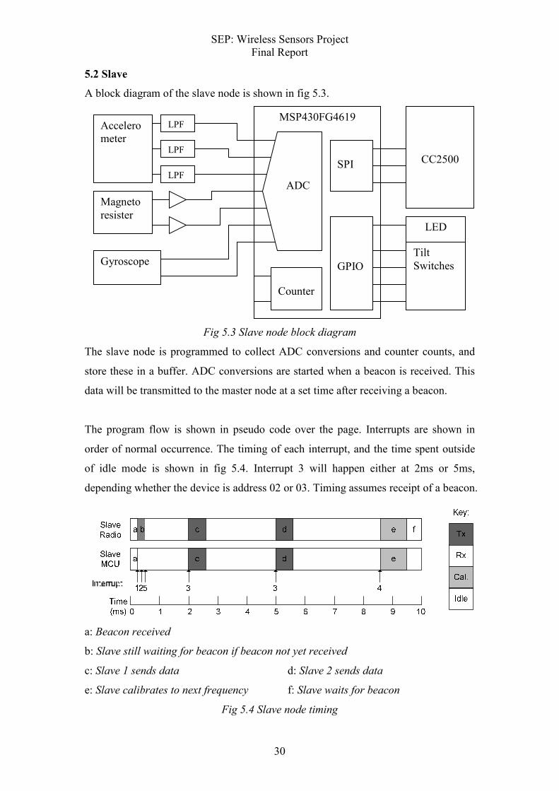
5.2 Slave
A block diagram of the slave node is shown in fig 5.3.
Fig 5.3 Slave node block diagram
The slave node is programmed to collect ADC conversions and counter counts, and
store these in a buffer. ADC conversions are started when a beacon is received. This
data will be transmitted to the master node at a set time after receiving a beacon.
The program flow is shown in pseudo code over the page. Interrupts are shown in
order of normal occurrence. The timing of each interrupt, and the time spent outside
of idle mode is shown in fig 5.4. Interrupt 3 will happen either at 2ms or 5ms,
depending whether the device is address 02 or 03. Timing assumes receipt of a beacon.
a: Beacon received
b: Slave still waiting for beacon if beacon not yet received
c: Slave 1 sends data d: Slave 2 sends data
e: Slave calibrates to next frequency f: Slave waits for beacon
Fig 5.4 Slave node timing
Counter
Accelerometer
Magneto
resister
LPF
LPF
LPF
MSP430FG4619
CC2500
SPI
Gyroscope
ADC
GPIO
Tilt
Switches
LED
SEP: Wireless Sensors Project Final Report
31
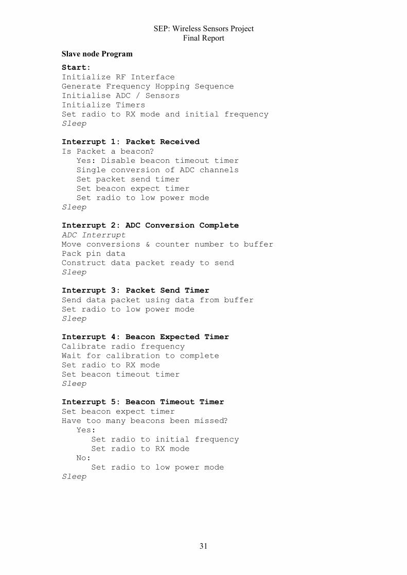
Slave node Program
Start:
Initialize RF Interface
Generate Frequency Hopping Sequence
Initialise ADC / Sensors
Initialize Timers
Set radio to RX mode and initial frequency
Sleep
Interrupt 1: Packet Received
Is Packet a beacon?
Yes: Disable beacon timeout timer
Single conversion of ADC channels
Set packet send timer
Set beacon expect timer
Set radio to low power mode
Sleep
Interrupt 2: ADC Conversion Complete
ADC Interrupt
Move conversions & counter number to buffer
Pack pin data
Construct data packet ready to send
Sleep
Interrupt 3: Packet Send Timer
Send data packet using data from buffer
Set radio to low power mode
Sleep
Interrupt 4: Beacon Expected Timer
Calibrate radio frequency
Wait for calibration to complete
Set radio to RX mode
Set beacon timeout timer
Sleep
Interrupt 5: Beacon Timeout Timer
Set beacon expect timer
Have too many beacons been missed?
Yes:
Set radio to initial frequency
Set radio to RX mode
No:
Set radio to low power mode
Sleep

SEP: Wireless Sensors Project Final Report
32
5.3 PC Software
Several PC programs were written to utilise the sensor nodes. Sensorman is a program
which reads the sensor data in from the com port, and forwards the data over the
network API as it is received. SyncAsync is a program which takes data from
Sensorman and buffers it. This data is then released upon the receipt of a request from
another program. SensorDisplay1 and 2 are programs which use Sensorman to display
the sensor data from nodes 1 and 2 respectively. Sensor display also provides example
algorithms for interpreting the sensor results.
All of the above programs utilise the Network API, developed by Ahmed Aichi in the
previous year of the SEP, to pass data between one another. The ports and link names
used on the network API are given in Appendix C.
SEP: Wireless Sensors Project Final Report
33
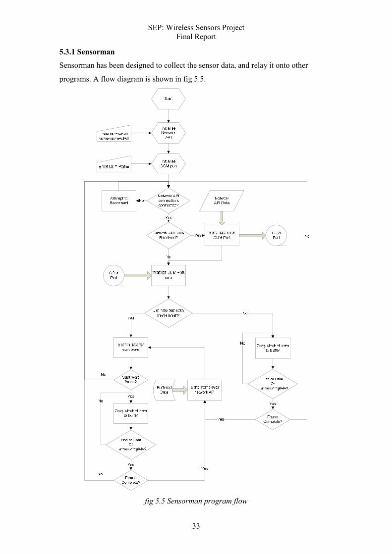
5.3.1 Sensorman
Sensorman has been designed to collect the sensor data, and relay it onto other
programs. A flow diagram is shown in fig 5.5.
fig 5.5 Sensorman program flow

SEP: Wireless Sensors Project Final Report
34
Once the sensor readings have been collected by the master node, they need to be
communicated to the PC. A USB link to the PC has been created using a RS232 to
USB converter. This converter acts as a COM port, allowing the PC to communicate
to the master using a COM port program. This was achieved using a COM-port
library, which is free under the GNU license [10]. Microsoft Visual Studio was used
to create several PC programs to collect and use the sensor data.
Firstly, the protocol for data transfer between the PC and the master node needed to
be defined. The Master node sends data to the PC as it becomes available. It is sent in
the same format as a packet of data is sent over the wireless network, except without
the preamble, CRC check or other wireless related overhead. Instead the data to be
sent is preceded by 2 chars (2*8 bits) of ASCII "II" . The packet format is given in
table 5.1.
Section Length (bits) *Header Length
Start word "II" 16 Node Address 8
Dest. Address 8 Battery Remaining 3
Header* 16 Reserved 5
Port 1 .. 13** 16 per port ** Port 1..13 Length
Reserved 3
GPIO state 1
Sensor Value 12
Table 5.1 packet format for data received by sensorman
The ASCII sequence "II" is used by the PC interface program to identify the start of a
data packet. This sequence is unique to the start identifier under the current protocol
(it cannot occur in the data stream). The same is true for the stop sequence. Once the
start sequence has been identified, the following received data is assumed to be the
data packet. If a packet is partially retrieved, then the next data bytes to be received
are assumed to be the continuation of the data packet. Once the data has been
successfully received by the program, it is sent over the network API. Each wireless
node has its own 'link' on the network API. The data is sent as a string with each
section delimited by spaces, in the formant shown in table 5.2.

SEP: Wireless Sensors Project Final Report
35
Section Allowed values
Command "realdata"
Number of Arguments 26
Port 1 ADC 0 .. 4095
Port 1 Pin 0 .. 1
… …
Port 13 ADC 0 .. 4095
Port 13 Pin 0 .. 1
Table 5.2 Packet format for data sent by sensorman
In table 3.8, the command "realdata" can be used by the receiving program to ensure
that a correct packet of data is being received.
The data for each node is sent as soon as it is received from the master. The program
receiving the data over the network API must handle the data fast enough, such that
the network API receive buffer does not overflow. In the event of a lost network
connection, the program stops until the link is re-established. The program flow is
shown in appendix I. Commands to be sent to the nodes must come from the network
API link of the node as a string in the format shown in table 5.3, with sections
delimited by spaces.
Section Allowed values
Command "command"
Number of Arguments 2
Command 0..8
Port number 1..13
Table 5.3 Packet format for commands received by sensorman
The command is then sent to the master node by the program in the format shown in
table 5.4.
Section Length (bits)
Start word "UU" 16
Command Address 8
Command 8
Port number 8
Table 5.4 Packet format for commands sent by sensorman

SEP: Wireless Sensors Project Final Report
36
5.3.2 SyncAsync
SyncAsync is a program which was written to convert the synchronous data stream
from Sensorman into an asynchronous data stream, where node data is available on
request. It has been tailored for use with the SEP project. The program flow is shown
in fig 5.6.
fig 5.6 SyncAsync program flow

SEP: Wireless Sensors Project Final Report
37
SyncAsync must have one instance for each data stream which is to be converted.
Data is taken in from Sensorman, and stored in a buffer. This buffer is 500 readings
large, so the program can continue to buffer data for 5 seconds before an overflow
occurs.
A program should be connected to SyncAsync, which requests data from the program.
Upon receipt of a data request, the buffered ADC values for Ports 1 to 11 are
averaged. The count values from ports 12 to 13 are summed. The latest port pin
values are taken. This data is then sent to the receiving program in the same format
that Sensorman used (see table 3.8). If a buffer overflow has occurred, the receiving
program will be notified, and all buffered values will be discarded; freeing the buffer.
Commands are received from the receiving program in the same format as used by
Sensorman (see table 3.9). These are then forwarded to Sensorman.
SEP: Wireless Sensors Project Final Report
38
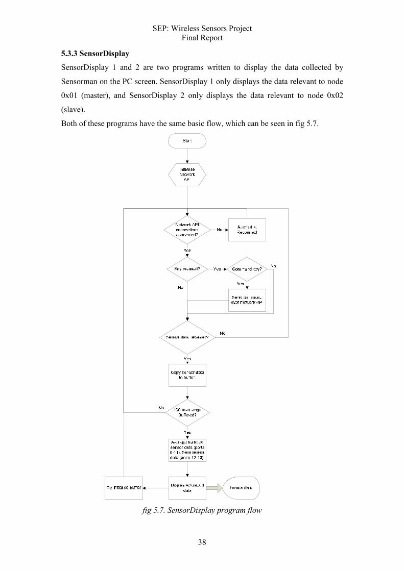
5.3.3 SensorDisplay
SensorDisplay 1 and 2 are two programs written to display the data collected by
Sensorman on the PC screen. SensorDisplay 1 only displays the data relevant to node
0x01 (master), and SensorDisplay 2 only displays the data relevant to node 0x02
(slave).
Both of these programs have the same basic flow, which can be seen in fig 5.7.
fig 5.7. SensorDisplay program flow
SEP: Wireless Sensors Project Final Report
39
SensorDisplay 1 allows the user to toggle the LED on the node, and set the port pins 5
to 8 to inputs or outputs, and set them high or low. It is also possible to set the
accelerometer sensitivity. The program uses the magneto-resistor, accelerometer,
speed and distance-travelled algorithms.
SensorDisplay 2 allows the user to toggle the LED on the node. It is also possible to
set the accelerometer sensitivity. The program uses the magneto-resistor and
accelerometer algorithms.
Algorithms
The code for all algorithms is given in Appendix D.
int magnetoresistor(int fieldA, int fieldB)
This algorithm reads in two magnetoresistor field values, and returns the direction the
part is facing (in degrees). The algorithm is calibrated using the #define values in the
header file:
minMGRvalue; sets the minimum possible value.
maxMGRvalue; sets the maximum possible value.
MGRmargin; sets the noise margins for the max and min values.
MGRAmult; field A is multiplied by this value to scale field A to the maxMGRvalue.
MGRBmult; field B is multiplied by this value to scale field B to the maxMGRvalue.
void accelerometer(int Xin, int Yin, int Zin, int Gsel1, int Gsel2, int* Xout, int*
Yout, int* Zout)
This algorithm reads in the three accelerometer values, the g-select settings and three
output value addresses. The three accelerometer values are converted to their value in
g's, and this is written to the three output values.
int speed(int count)
This algorithm will take the number of counts collected, and convert it to a speed in
m/s. This speed will be returned. It is assumed that the count value is from 10ms. The
algorithm is calibrated using the #define values in the header file:
wheelDiameter; the diameter of the wheel (in mm)
numberOfSpokes; the number of spokes on the wheel encoder

SEP: Wireless Sensors Project Final Report
40
int distanceTravelled(int count)
This algorithm will take the number of counts collected, and convert it to a distance in
mm. The distance will be returned. The algorithm is calibrated using the #define
values in the header file:
wheelDiameter; the diameter of the wheel (in mm)
numberOfSpokes; the number of spokes on the wheel encoder

SEP: Wireless Sensors Project Final Report
41
6. Hardware
6.1 Sensors
Sensors with an analogue output will be connected to the ADC on the MSP430. Other
sensors will connect to a GPIO pin on the MSP430. The MSP430's ADC can measure
a voltage between 0-3Vpp, single ended. Therefore, some sensors need an analogue
interface to convert the sensor output to the correct format.
6.1.1 Accelerometer
The accelerometer (Freescale, MMA7260QT) was tested to measure the sensor's
response to gravity along each axis. The accelerometer was set to the most sensitive
setting, and the output measured using the circuit in fig 6.1. The outputs have been
filtered as suggested in the accelerometer datasheet. The results are given in table 6.1.
fig 6.1 Accelerometer test circuit
Axis -1G 0G 1G
X 0.87 V 1.6 V 2.37 V
Y 0.92 V 1.7 V 2.47 V
Z 0.73 V 1.45 V 2.26 V
Table 6.1 Accelerometer response to gravity
The output was also viewed on an oscilloscope, and it was observed that there was no
ringing or noise on the outputs.
From these results, it was concluded that no further signal conditioning needed to be
performed on the sensor.

SEP: Wireless Sensors Project Final Report
42
6.1.2 Odometer
The output of the odometer (from Active-Robots) is a 5V logic signal. This is
incompatible with the MSP430 GPIO pins, therefore the signal must be reduced to a
3V logic signal. This has been achieved using the circuit in fig 6.2. The odometer will
be connected to a 'counter' on the MSP430, and the number of level transitions will be
measured and transmitted.
Fig 6.2 Logic level converter circuit
The working distance between the encoding wheel and sensor has been tested. The
separation must be between 1mm and 3mm.
6.1.3 Magneto Resistor
The magneto resistor (Honeywell HMC1002) has a differential output, with the
difference between the two terminals being approximately 20mV due to the earths
magnetic field. Therefore, the output from each field needs to be converted to a 0-3V
single ended signal, for use with the MSP430.
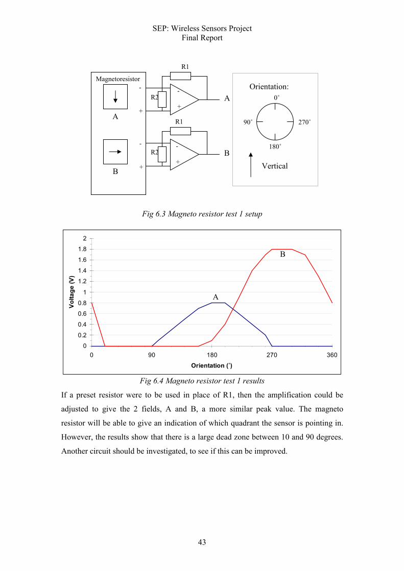
Test 1:
The circuit shown in fig 6.3 was designed to convert the output of the magneto
resistor to a single ended format. The output has been measured for R1 = 100K, and
R2 = 10K. This gives an output as shown in fig 6.4.
Odometer
5V supply
3.3V supply
Output'
GND
Output
GND
5V
10K
1N4148
SEP: Wireless Sensors Project Final Report
43
Fig 6.3 Magneto resistor test 1 setup
Fig 6.4 Magneto resistor test 1 results
If a preset resistor were to be used in place of R1, then the amplification could be
adjusted to give the 2 fields, A and B, a more similar peak value. The magneto
resistor will be able to give an indication of which quadrant the sensor is pointing in.
However, the results show that there is a large dead zone between 10 and 90 degrees.
Another circuit should be investigated, to see if this can be improved.
0
0.2
0.4
0.6
0.8
1
1.2
1.4
1.6
1.8
2
0 90 180 270 360
Orientation (˚)
Voltage (V)
A
B
R1
R2
R1
R2 -
+
-
+
Magnetoresistor
A
B
-
+
-
+
A
B
90˚
Orientation:
Vertical
0˚
180˚
270˚
SEP: Wireless Sensors Project Final Report
44
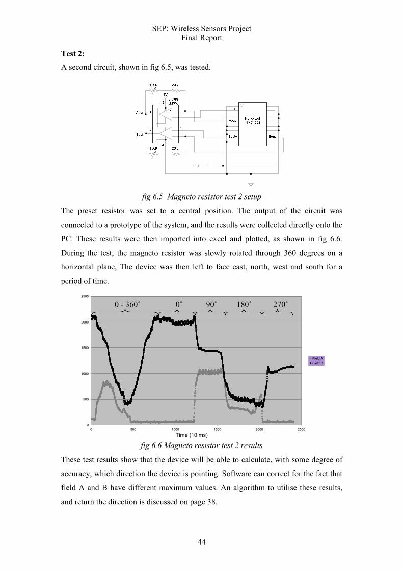
Test 2:
A second circuit, shown in fig 6.5, was tested.
fig 6.5 Magneto resistor test 2 setup
The preset resistor was set to a central position. The output of the circuit was
connected to a prototype of the system, and the results were collected directly onto the
PC. These results were then imported into excel and plotted, as shown in fig 6.6.
During the test, the magneto resistor was slowly rotated through 360 degrees on a
horizontal plane, The device was then left to face east, north, west and south for a
period of time.
0
500
1000
1500
2000
2500
0 500 1000 1500 2000 2500
Field A
Field B
fig 6.6 Magneto resistor test 2 results
These test results show that the device will be able to calculate, with some degree of
accuracy, which direction the device is pointing. Software can correct for the fact that
field A and B have different maximum values. An algorithm to utilise these results,
and return the direction is discussed on page 38.
0 - 360˚
Time (10 ms)
0˚ 90˚ 180˚ 270˚
SEP: Wireless Sensors Project Final Report
45
6.2 PC interface hardware
Communications to the PC are achieved by a device which simulates a RS232 COM
Port. The UART communications of the MSP430 uses a 0-3V inverted signal. The
RS232 from the device operates at -15V to +15V, non-inverted. Therefore, an
interface had to be designed to connect the RS232 device to the MSP430.
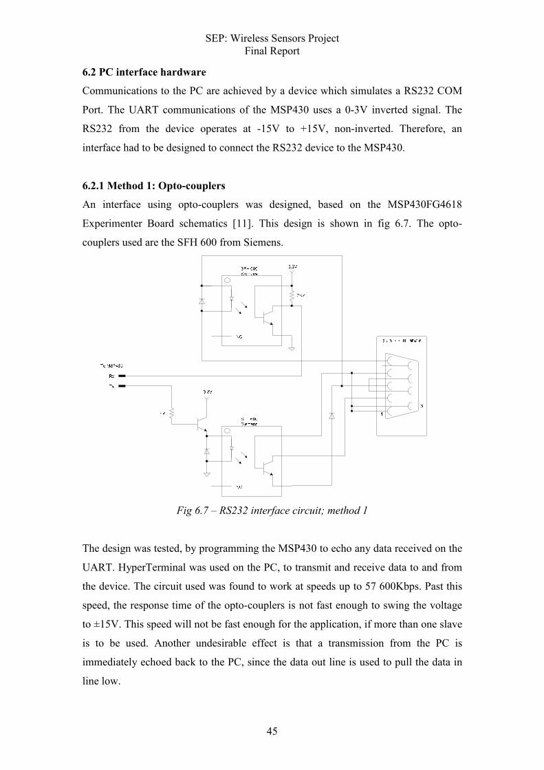
6.2.1 Method 1: Opto-couplers
An interface using opto-couplers was designed, based on the MSP430FG4618
Experimenter Board schematics [11]. This design is shown in fig 6.7. The opto-
couplers used are the SFH 600 from Siemens.
Fig 6.7 – RS232 interface circuit; method 1
The design was tested, by programming the MSP430 to echo any data received on the
UART. HyperTerminal was used on the PC, to transmit and receive data to and from
the device. The circuit used was found to work at speeds up to 57 600Kbps. Past this
speed, the response time of the opto-couplers is not fast enough to swing the voltage
to ±15V. This speed will not be fast enough for the application, if more than one slave
is to be used. Another undesirable effect is that a transmission from the PC is
immediately echoed back to the PC, since the data out line is used to pull the data in
line low.

SEP: Wireless Sensors Project Final Report
46
6.2.2 Method 2: RS232 Driver / Receiver
Because method 1 didn't provide a suitable solution for the RS232 interface, the use
of a RS232 Driver/Receiver was investigated. A circuit to use the MAX3232 CDBR
from Texas Instruments was designed. This circuit is shown in fig 6.8.
Fig 6.8 - RS232 interface circuit; method 2
The circuit was tested, by programming the MSP430 to echo any data received on the
UART. HyperTerminal was used on the PC, to transmit and receive data to and from
the device. The circuit used was found to work at speeds up to 460 800Kbps. Unlike
method 1, there is no immediate echo of transmitted data. This circuit is fast enough
to be used in the final design.
SEP: Wireless Sensors Project Final Report
47
6.3 Power Management
Because the PC will communicate to the master via USB, it is desirable to power the
master node from the USB supply. This means a 5V to 3.3V DC/DC converter is
required. The TPS60501 from Texas Instruments (TI) was found to meet the
specifications. Samples of the device were obtained for free using TI's online sample
program.
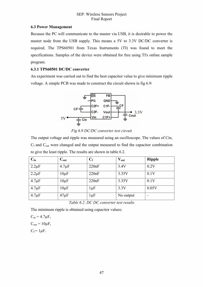
6.3.1 TPS60501 DC/DC converter
An experiment was carried out to find the best capacitor value to give minimum ripple
voltage. A simple PCB was made to construct the circuit shown in fig 6.9:
Fig 6.9 DC/DC converter test circuit
The output voltage and ripple was measured using an oscilloscope. The values of Cin,
Cf and Cout were changed and the output measured to find the capacitor combination
to give the least ripple. The results are shown in table 6.2.
Cin Cout Cf Vout Ripple
2.2µF 4.7µF 220nF 3.4V 0.2V
2.2µF 10µF 220nF 3.35V 0.1V
4.7µF 10µF 220nF 3.35V 0.1V
4.7µF 10µF 1µF 3.3V 0.05V
4.7µF 47µF 1µF No output -
Table 6.2. DC DC converter test results
The minimum ripple is obtained using capacitor values;
Cin = 4.7µF,
Cout = 10µF,
Cf = 1µF.
5V
3.3V
SEP: Wireless Sensors Project Final Report
48
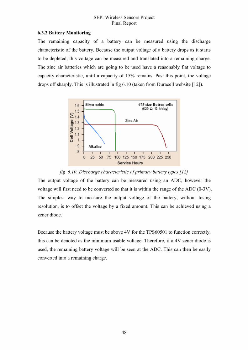
6.3.2 Battery Monitoring
The remaining capacity of a battery can be measured using the discharge
characteristic of the battery. Because the output voltage of a battery drops as it starts
to be depleted, this voltage can be measured and translated into a remaining charge.
The zinc air batteries which are going to be used have a reasonably flat voltage to
capacity characteristic, until a capacity of 15% remains. Past this point, the voltage
drops off sharply. This is illustrated in fig 6.10 (taken from Duracell website [12]).
fig 6.10. Discharge characteristic of primary battery types [12]
The output voltage of the battery can be measured using an ADC, however the
voltage will first need to be converted so that it is within the range of the ADC (0-3V).
The simplest way to measure the output voltage of the battery, without losing
resolution, is to offset the voltage by a fixed amount. This can be achieved using a
zener diode.
Because the battery voltage must be above 4V for the TPS60501 to function correctly,
this can be denoted as the minimum usable voltage. Therefore, if a 4V zener diode is
used, the remaining battery voltage will be seen at the ADC. This can then be easily
converted into a remaining charge.
SEP: Wireless Sensors Project Final Report
49
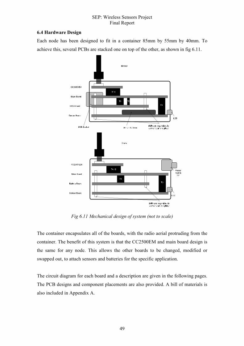
6.4 Hardware Design
Each node has been designed to fit in a container 85mm by 55mm by 40mm. To
achieve this, several PCBs are stacked one on top of the other, as shown in fig 6.11.
Fig 6.11 Mechanical design of system (not to scale)
The container encapsulates all of the boards, with the radio aerial protruding from the
container. The benefit of this system is that the CC2500EM and main board design is
the same for any node. This allows the other boards to be changed, modified or
swapped out, to attach sensors and batteries for the specific application.
The circuit diagram for each board and a description are given in the following pages.
The PCB designs and component placements are also provided. A bill of materials is
also included in Appendix A.

SEP: Wireless Sensors Project Final Report
50
6.4.1 Main Board
4
1
3
5
7
9
11
JTAG
Header
5
10
15
20
2530 35 40 45 50
55
60
65
70
7580859095100
Texas Instruments
MSP430 FG4619
100 PZ Package
10nF
47K
VCC
ADC3
ADC4
ADC5
ADC6
ADC7
Xout
Xin
ADC12
ADC13
ADC14
ADC15
32KHz
10K
S1
S2
S3
S4
S5
S6
S7
S8S9
DIP
Switch
Count1
Count2
P13
Texas
Instruments
TPS60501
4.7µF
1µF
10µF
1µF3.3V
C1F-
C1F+
GND
FB
5V
C2F+
C2F-
/EN
T4T5
11
3.3V
3.3V
GND
SOMI
SIMO
SCLK
CSn
GDO2
GDO1
CSn
5V
T1
1
T2
1
1P1
P2
P3
P4
P5
P6
P7
P8
P9
P10
P11
P12
P13
5V
3.3V GND
T3
T1: Input of 5V and GND
T2: Output of 3.3V and GND. Connects to RS232 device.
T3: Port pin inputs/outputs. Sensor inputs. 5V, 3.3V and GND output.
T4 / T5: To connect to CC2500 EM P1 and P2 respectively.
JTAG header: Used for programming MSP430
Fig 6.12 Main Board circuit diagram
SEP: Wireless Sensors Project Final Report
51
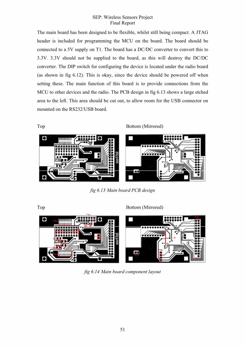
The main board has been designed to be flexible, whilst still being compact. A JTAG
header is included for programming the MCU on the board. The board should be
connected to a 5V supply on T1. The board has a DC/DC converter to convert this to
3.3V. 3.3V should not be supplied to the board, as this will destroy the DC/DC
converter. The DIP switch for configuring the device is located under the radio board
(as shown in fig 6.12). This is okay, since the device should be powered off when
setting these. The main function of this board is to provide connections from the
MCU to other devices and the radio. The PCB design in fig 6.13 shows a large etched
area to the left. This area should be cut out, to allow room for the USB connector on
mounted on the RS232/USB board.
Top Bottom (Mirrored)
fig 6.13 Main board PCB design
Top Bottom (Mirrored)
fig 6.14 Main board component layout

SEP: Wireless Sensors Project Final Report
52
6.4.2 Master: RS232/USB Board
T1: output of 5V and GND
T2: input of 3.3V and GND. Tx/Rx used for RS232 communications.
USB B Female socket: Used for USB communications with PC.
Fig 6.15 RS232/USB board circuit diagram
This board converts USB communications from the PC to a UART communication
usable with the MCU. It also provides a 5V power supply, taken from the USB. It
uses a RS232/USB converter, and a RS232 level shifter, shown in fig 6.15. In figures
6.16 and 6.17, the large rectangular area marked "ee41al" should be removed to allow
room for the RS232/USB converter.

SEP: Wireless Sensors Project Final Report
53
Top Bottom (Mirrored)
fig 6.16 RS232/USB board PCB design
Top Bottom (Mirrored)
fig 6.17 RS232/USB board component layout
SEP: Wireless Sensors Project Final Report
54
6.4.3 Slave: Battery Board
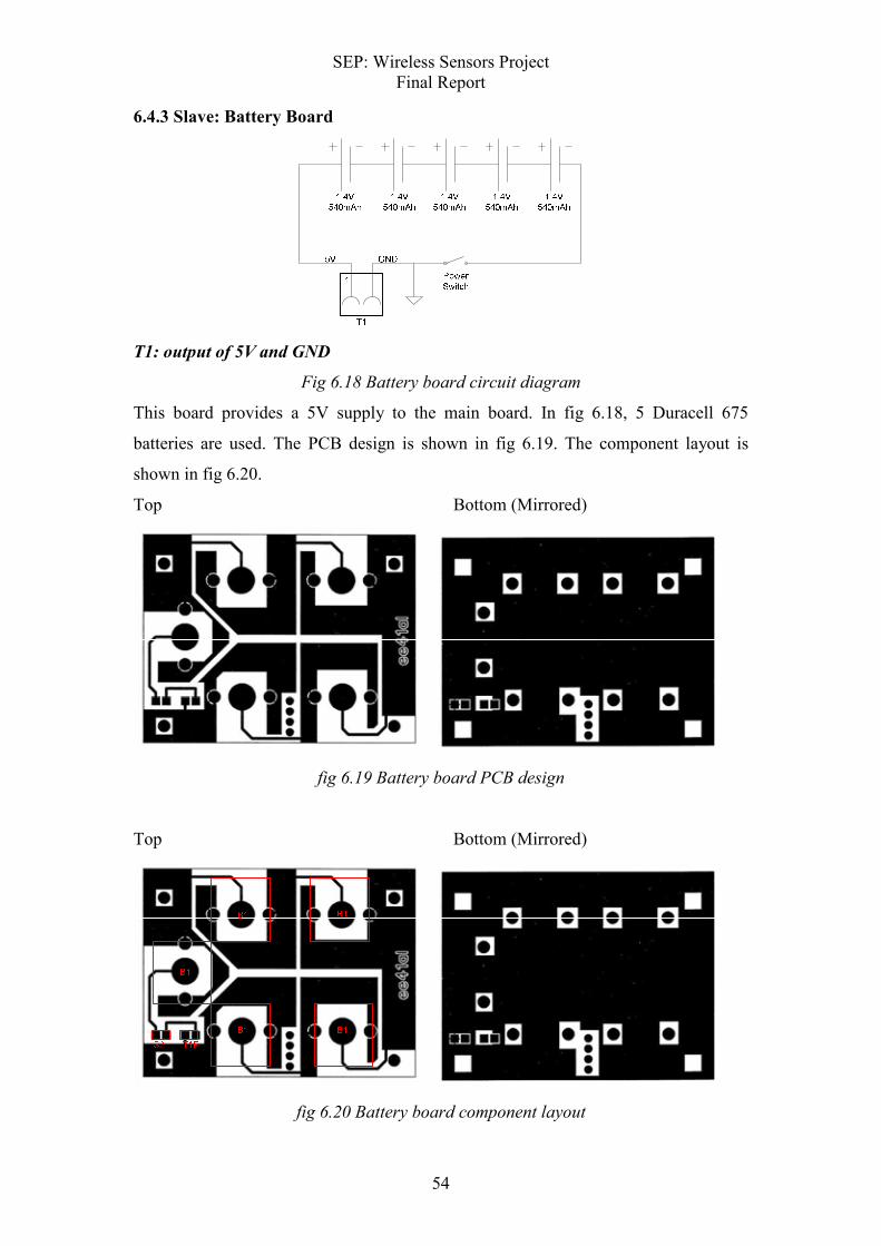
T1: output of 5V and GND
Fig 6.18 Battery board circuit diagram
This board provides a 5V supply to the main board. In fig 6.18, 5 Duracell 675
batteries are used. The PCB design is shown in fig 6.19. The component layout is
shown in fig 6.20.
Top Bottom (Mirrored)
fig 6.19 Battery board PCB design
Top Bottom (Mirrored)
fig 6.20 Battery board component layout
SEP: Wireless Sensors Project Final Report
55
6.4.4 Master: Sensor board
Xout
Yout
Zout
100R
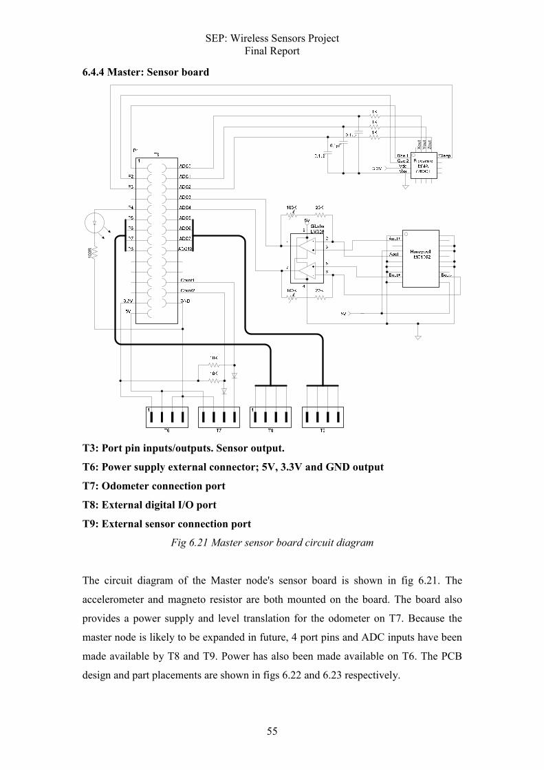
T3: Port pin inputs/outputs. Sensor output.
T6: Power supply external connector; 5V, 3.3V and GND output
T7: Odometer connection port
T8: External digital I/O port
T9: External sensor connection port
Fig 6.21 Master sensor board circuit diagram
The circuit diagram of the Master node's sensor board is shown in fig 6.21. The
accelerometer and magneto resistor are both mounted on the board. The board also
provides a power supply and level translation for the odometer on T7. Because the
master node is likely to be expanded in future, 4 port pins and ADC inputs have been
made available by T8 and T9. Power has also been made available on T6. The PCB
design and part placements are shown in figs 6.22 and 6.23 respectively.

SEP: Wireless Sensors Project Final Report
56
Top Bottom (Mirrored)
fig 6.22 Master sensor board PCB design
Top Bottom (Mirrored)
fig 6.23 Master sensor board component layout

SEP: Wireless Sensors Project Final Report
57
6.4.5 Slave: Sensor board
Freescale
MMA
7260QT
Xout
Yout
Zout
/SleepGsel1
Gsel2
Vdd
Vss
1K
1K
1K0.1µF
0.1µF
0.1µF
Honeywell
HMC1002
Aout+
Aout-
Bout-Bout+
5V
4
8
1
7
2
3
6
5
SiLabs
LM358
-
+
+
-
100K 20K
100K 20K
5V
T3
1
GND
5V
3.3V
3.3V
100R
P2
P3
P4
P5
P6
P7
P8
ADC0
ADC1
ADC2
ADC3
ADC4
ADC5
ADC6
ADC13
P1
Sparkfun
IDG300
Breakout
3.3V
GND
Vref
Axis1
Axis2
0 ohm
3V9
Zener
Mercury
Switch
Mercury
Switch
Mercury
Switch
Mercury
Switch
10K
10K
10K
10K
T3: Port pin inputs/outputs. Sensor output.
Fig 6.24 Slave sensor board circuit diagram

SEP: Wireless Sensors Project Final Report
58
Unlike the master sensor board, the slave sensor board shown in fig 6.24 doesn't have
any external connectors. Only T3 is used, for connection to the main board. In
addition to the accelerometer and magneto resistor, this board also includes a
gyroscope and 4 tilt switches. The tilt switches will break the connection to ground if
the board is tilted more than 15˚ from horizontal. This has been included as a hard
indication if the UAV is tilting too much. The PCB design and part placements are
shown in figs 6.25 and 6.26 respectively.
Top Bottom (Mirrored)
fig 6.25 Slave sensor board PCB design
Top Bottom (Mirrored)
fig 6.26 Slave sensor board component layout

SEP: Wireless Sensors Project Final Report
59
7. Discussions
7.1 Project Status
At the time of writing the report, a prototype system has been successfully tested.
Wireless sensor data can be transmitted wirelessly to the PC, and displayed on screen.
The final system is yet to be finished, because difficulties were encountered while
assembling the main boards. The hand soldering of the 100 pin surface mount MCU
proved to be problematic. All other boards have been assembled and tested
successfully.
7.2 Estimated total cost
The cost of this project has been severely reduced, since most of the parts were
donated or obtained at no cost. Several gyroscopes have been ordered, because one
was destroyed during testing, which dramatically increased the cost of the project.
Parts Purchased:
PCB's: ₤10.82
SMT Headers: ₤21.75
Gyroscopes: ₤165.00
Wheel encoder set: ₤37.26
Magneto Resistors: ₤35.51
USB Adapter: ₤22.40
Misc. parts ₤57.60
Total: ₤360.34

SEP: Wireless Sensors Project Final Report
60
7.3 Objectives Achieved
The objectives stated in section 1.3 (page 2) are:
Primary:
-Create a wireless data transmission system
This objective has been achieved. A wireless data protocol has been designed
and implemented, using a synchronous TDMA approach.
-Collect sensor data
This objective has been achieved. Sensor data is collected using ADC's,
counters and GPIO pins. An example of interpreting this data has also been written in
software (SensorDisplay 1&2).
-Communicate data to the PC
This objective has been achieved. Sensor data is sent to the PC using a virtual
COM port. Example programs for collecting and forwarding the data have also been
written (Sensorman, SyncAsync).
Secondary:
-Implement a frequency scan
This has not been achieved.
-Implement frequency hopping
This objective has been achieved. The wireless system utilises 40 channels
over the 2.4 to 2.4835 GHz frequency range. The system also complies with ETSI
standards.
-Provide an estimation of distance between nodes
This has not been achieved.
-Implement a battery level monitor
This objective has been achieved. The battery remaining, when below 15%, is
observed by using an ADC port.
All of the primary objectives have been achieved, and two of four secondary
objectives have been achieved.

SEP: Wireless Sensors Project Final Report
61
7.4 Gantt chart
Fig 7.1 shows a Gantt chart of the original work plan. The intended schedule is shown
in green. The actual schedule is indicated in blue. There was some delay in the arrival
of the hardware, hence initial testing did not begin until week 8.
Semester1 Week 5 6 7 8 9 10 11 12 13 Exams and holidays
Define project and set objectives 1
Research and order development platform 2
Create RF Link 3
Test RF comms to find most suitable method
State machine diagram
Coding and testing
annotation
Deliver: Prototype of RF Link
Code peripherals for interfacing hardware 3 4
State machine diagram
Coding
Testing
Deliver: Prototype of sensor data collection
Overall system design 5
State diagram
Coding and testing
Annotation
Deliver: Prototype any-sensor connection
Link to PC 6
assemble USB I2C link
define communications protocol
testing
Deliver: Prototype collection of data by PC
Hardware Design 6.1, 4 7
Power Management
External interface design
PCB design
Mechanical design
Interim Report 8
Collection of results into appendices
Experimental work
Write up introduction, conclusion
References
Contents
Semester2 Week 1 2 3 4 5 6 7 8 9 10-13
Deadline: Interim Report 8 Time for overrun
Hardware Design 7 9
Construction and testing
Deliver: Create portable wireless sensor interface
Integration onto chassis 9 10
Deliver: Install hardware on platform and UAV
Final Report 8 11
Integration of tests and results
Integration of any new designs
Update conclusions
References
Diagrams
Documentation
Deadline: Final Report
fig 7.1 Preliminary Gantt chart
Therefore a revised Gantt chart, shown in fig 7.2, was made in January. Again, the
intended schedule is shown in green. The actual schedule is indicated in blue.
Many deadlines proved too optimistic; most notably creating the link to the PC (6),
which overran by a considerable amount. However, this did not cause a problem,
since several weeks were planned for the overrun of tasks. Another area which has
taken longer than expected is the construction of the final hardware. This has overrun
because of the difficulty experienced is assembling the main board.
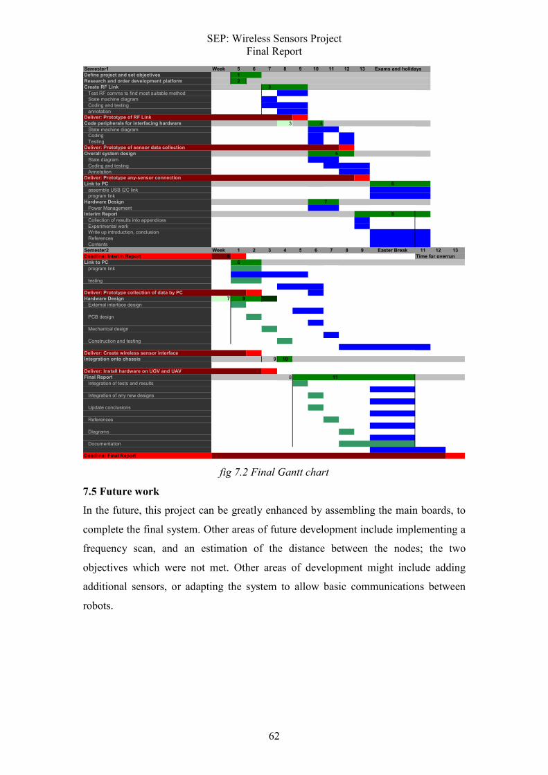
SEP: Wireless Sensors Project Final Report
62
Semester1 Week 5 6 7 8 9 10 11 12 13 Exams and holidays
Define project and set objectives 1
Research and order development platform 2
Create RF Link 3
Test RF comms to find most suitable method
State machine diagram
Coding and testing
annotation
Deliver: Prototype of RF Link
Code peripherals for interfacing hardware 3 4
State machine diagram
Coding
Testing
Deliver: Prototype of sensor data collection
Overall system design 5
State diagram
Coding and testing
Annotation
Deliver: Prototype any-sensor connection
Link to PC 6
assemble USB I2C link
program link
Hardware Design 7
Power Management
Interim Report 8
Collection of results into appendices
Experimental work
Write up introduction, conclusion
References
Contents
Semester2 Week 1 2 3 4 5 6 7 8 9 Easter Break 11 12 13
Deadline: Interim Report 8 Time for overrun
Link to PC 6
program link
testing
Deliver: Prototype collection of data by PC
Hardware Design 7 9
External interface design
PCB design
Mechanical design
Construction and testing
Deliver: Create wireless sensor interface
Integration onto chassis 9 10
Deliver: Install hardware on UGV and UAV
Final Report 8 11
Integration of tests and results
Integration of any new designs
Update conclusions
References
Diagrams
Documentation
Deadline: Final Report
fig 7.2 Final Gantt chart
7.5 Future work
In the future, this project can be greatly enhanced by assembling the main boards, to
complete the final system. Other areas of future development include implementing a
frequency scan, and an estimation of the distance between the nodes; the two
objectives which were not met. Other areas of development might include adding
additional sensors, or adapting the system to allow basic communications between
robots.

SEP: Wireless Sensors Project Final Report
63
References
[1] Wireless Information Networks (2nd edition)
Written by Kaveh Pahlavan and Allen H Levesque
Published by John Wiley and Sons Inc.
[2] Ad Hoc Wireless Networks; Architectures and Protocols
Written by C Siva Ram Murthy and B S Manoj
Published by Prentice Hall
[3] Hacking; The Art of Exploitation
Written by Jon Erickson
Published by No Starch Press
[4] ETSI: EN 300 220; European Standard, version 2.1.1
Author not declared
Published by ETSI
Available at http://www.etsi.org/
[5] ETSI: EN 300 328; European Standard, version 1.7.1
Author not declared
Published by ETSI
Available at http://www.etsi.org/
[6] “ZigBee Competitive Technology Analysis” Section Summary
Written by Prof. Dr.-Ing. Axel Sikora
Published by ZigBee organization
Available at http://www.zigbee.org/en/resources/whitepapers2.asp
[7] ZigBee and Wireless Radio Frequency Coexistence
Author not declared
Published by ZigBee organization
Available at http://www.zigbee.org/en/resources/whitepapers2.asp

SEP: Wireless Sensors Project Final Report
64
[8] Chipcon University Brochure
Written by A Lindsay
Published by Texas Instruments
Available at
http://www.ti.com/europe/docs/univ/download/ChipCon_Univ_Brochure_26July07.pdf
[9] MSP430 University Brochure
Written by A Lindsay
Published by Texas Instruments
Available at http://www.ti.com/europe/docs/univ/msp430unibrochure.pdf
[10] C++ Serial Port Library
Written by Ramon de Klein
Published by The Code Project
Available at http://www.codeproject.com/KB/system/serial.aspx
[11] MSP430FG4618/F2013 Experimenter’s Board Users Guide
Written by A Lindsay
Published by Texas Instruments
Available at http://focus.ti.com/lit/ug/slau213a/slau213a.pdf
[12] Duracell OEM website
Author not declared
Published by Procter & Gamble
Available at http://www.duracell.com/oem/
[13] Random number generation and Monte Carlo methods (2nd edition)
Written by James E. Gentle
Published by Springer

SEP: Wireless Sensors Project Final Report
65
Appendix A: Bill of Materials
Main Board
Code Qty Part
U1 2 MSP430FG4618 100PZ
U2 2 TPS60501
R0 2 47K sm 0806
R1 2 10K sm 0806
R2 2 10K sm 0806
R3 2 10K sm 0806
R4 2 10K sm 0806
R5 2 10K sm 0806
R6 2 10K sm 0806
R7 2 10K sm 0806
R8 2 10K sm 0806
R9 2 10K sm 0806
C1 2 10nF sm 0604
C2 2 4.7 µF sm 0806
C3 2 10 µF sm 0806
C4 2 1 µF sm 0604
C5 2 1 µF sm 0604
X1 2 32KHz crystal osc.
S1 2 18 pin DIP switch
T1M 2 1x2 Header
T2M 2 1x4 Header
T3M 2 7x2 +1 pin Header
T4M 2 10x2 SMT
T5M 2 10x2 SMT
T10 2 7x2 header
PCB1 2 Dual layer FR4

SEP: Wireless Sensors Project Final Report
66
Battery Board
Code Qty Part
T1F 1 1x2 socket
S2 1 SPST rocker switch
B1 5 627 battery holder
PBC2 1 Dual layer FR4
USB/RS232 Board
Code Qty Part
U3 1 Max3232 CDBR
U4 1 USB/RS232 converter
U9 1 Diode sm
C6 1 100nF sm 0604
C7 1 100nF sm 0604
C8 1 100nF sm 0604
C9 1 100nF sm 0604
T1F 1 1x2 socket
T2F 1 1x4 socket
T11 1 USB B Female socket
PCB3 Dual layer FR4
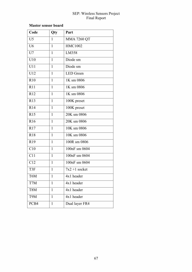
SEP: Wireless Sensors Project Final Report
67
Master sensor board
Code Qty Part
U5 1 MMA 7260 QT
U6 1 HMC1002
U7 1 LM358
U10 1 Diode sm
U11 1 Diode sm
U12 1 LED Green
R10 1 1K sm 0806
R11 1 1K sm 0806
R12 1 1K sm 0806
R13 1 100K preset
R14 1 100K preset
R15 1 20K sm 0806
R16 1 20K sm 0806
R17 1 10K sm 0806
R18 1 10K sm 0806
R19 1 100R sm 0806
C10 1 100nF sm 0604
C11 1 100nF sm 0604
C12 1 100nF sm 0604
T3F 1 7x2 +1 socket
T6M 1 4x1 header
T7M 1 4x1 header
T8M 1 4x1 header
T9M 1 4x1 header
PCB4 1 Dual layer FR4

SEP: Wireless Sensors Project Final Report
68
Slave sensor board
Code Qty Part
U5 1 MMA 7260 QT
U6 1 HMC1002
U7 1 LM358
U8 1 IDG300 Breakout
U12 1 LED Green
R10 1 1K sm 0806
R11 1 1K sm 0806
R12 1 1K sm 0806
R13 1 100K preset
R14 1 100K preset
R15 1 20K sm 0806
R16 1 20K sm 0806
R19 1 100R sm 0806
R20 1 10K sm 0806
R21 1 10K sm 0806
R22 1 10K sm 0806
R23 1 10K sm 0806
C10 1 100nF sm 0604
C11 1 100nF sm 0604
C12 1 100nF sm 0604
S3 1 Mercury tilt switch
S4 1 Mercury tilt switch
S5 1 Mercury tilt switch
S6 1 Mercury tilt switch
T3F 1 7x2 +1 socket
PCB4 1 Dual layer FR4
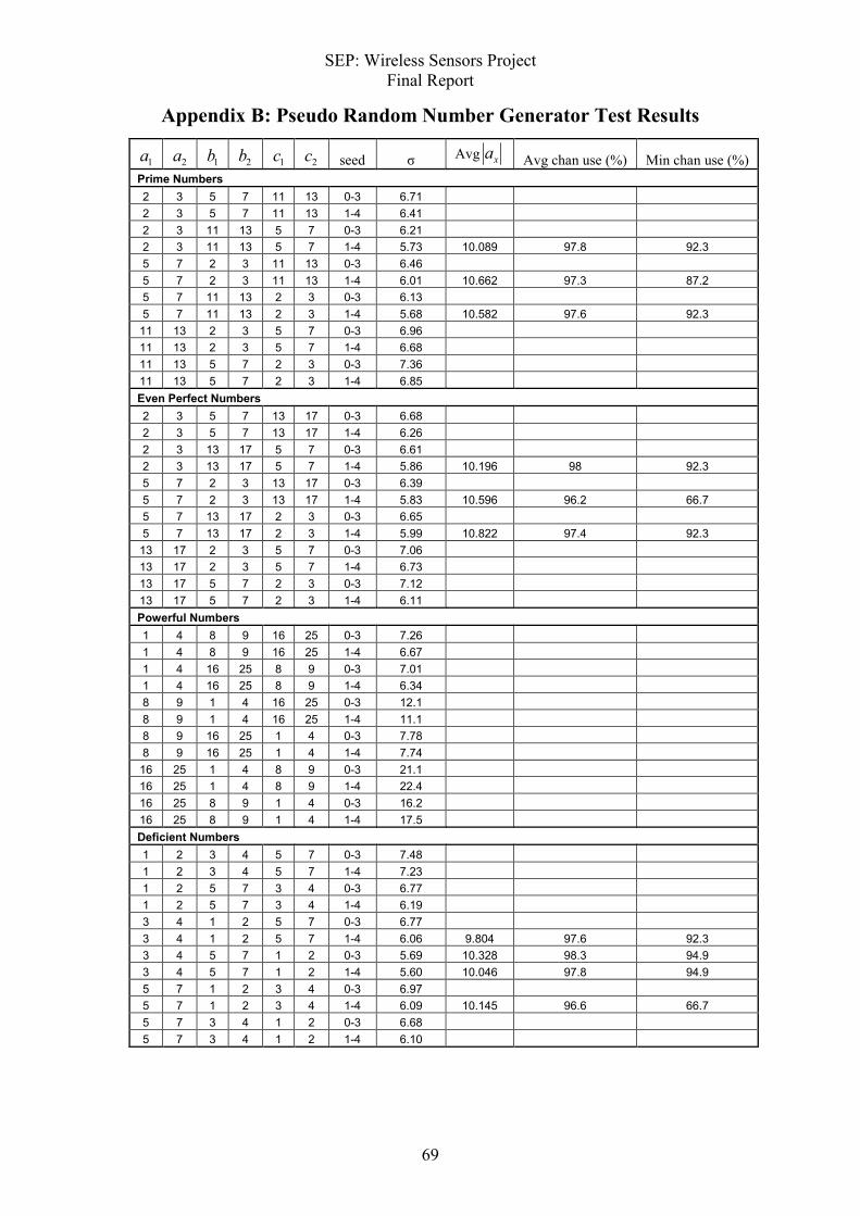
SEP: Wireless Sensors Project Final Report
69
Appendix B: Pseudo Random Number Generator Test Results
1a 2a 1b 2b 1c 2c seed σ Avg xa Avg chan use (%) Min chan use (%)
Prime Numbers
2 3 5 7 11 13 0-3 6.71
2 3 5 7 11 13 1-4 6.41
2 3 11 13 5 7 0-3 6.21
2 3 11 13 5 7 1-4 5.73 10.089 97.8 92.3
5 7 2 3 11 13 0-3 6.46
5 7 2 3 11 13 1-4 6.01 10.662 97.3 87.2
5 7 11 13 2 3 0-3 6.13
5 7 11 13 2 3 1-4 5.68 10.582 97.6 92.3
11 13 2 3 5 7 0-3 6.96
11 13 2 3 5 7 1-4 6.68
11 13 5 7 2 3 0-3 7.36
11 13 5 7 2 3 1-4 6.85
Even Perfect Numbers
2 3 5 7 13 17 0-3 6.68
2 3 5 7 13 17 1-4 6.26
2 3 13 17 5 7 0-3 6.61
2 3 13 17 5 7 1-4 5.86 10.196 98 92.3
5 7 2 3 13 17 0-3 6.39
5 7 2 3 13 17 1-4 5.83 10.596 96.2 66.7
5 7 13 17 2 3 0-3 6.65
5 7 13 17 2 3 1-4 5.99 10.822 97.4 92.3
13 17 2 3 5 7 0-3 7.06
13 17 2 3 5 7 1-4 6.73
13 17 5 7 2 3 0-3 7.12
13 17 5 7 2 3 1-4 6.11
Powerful Numbers
1 4 8 9 16 25 0-3 7.26
1 4 8 9 16 25 1-4 6.67
1 4 16 25 8 9 0-3 7.01
1 4 16 25 8 9 1-4 6.34
8 9 1 4 16 25 0-3 12.1
8 9 1 4 16 25 1-4 11.1
8 9 16 25 1 4 0-3 7.78
8 9 16 25 1 4 1-4 7.74
16 25 1 4 8 9 0-3 21.1
16 25 1 4 8 9 1-4 22.4
16 25 8 9 1 4 0-3 16.2
16 25 8 9 1 4 1-4 17.5
Deficient Numbers
1 2 3 4 5 7 0-3 7.48
1 2 3 4 5 7 1-4 7.23
1 2 5 7 3 4 0-3 6.77
1 2 5 7 3 4 1-4 6.19
3 4 1 2 5 7 0-3 6.77
3 4 1 2 5 7 1-4 6.06 9.804 97.6 92.3
3 4 5 7 1 2 0-3 5.69 10.328 98.3 94.9
3 4 5 7 1 2 1-4 5.60 10.046 97.8 94.9
5 7 1 2 3 4 0-3 6.97
5 7 1 2 3 4 1-4 6.09 10.145 96.6 66.7
5 7 3 4 1 2 0-3 6.68
5 7 3 4 1 2 1-4 6.10

SEP: Wireless Sensors Project Final Report
70
Appendix C: Network API Connections
Program Local name Port
Number
Link
Name
Inputs Outputs
Sensorman sensorman 12001 device1 commands sensor data
Sensorman sensorman 12002 device2 commands sensor data
Sensorman sensorman 12003 device3 commands sensor data
Sensorman sensorman 12004 device4 commands sensor data
SyncAsync sensordisplay 12001 device1 sensor data Commands
SyncAsync sensordisplay 12002 device2 sensor data Commands
SyncAsync sensordisplay 12003 device3 sensor data Commands
SyncAsync sensordisplay 12004 device4 sensor data Commands
SyncAsync sensordisplay 12008 syncasync Commands,
data requests
sensor data,
warnings
SyncAsync sensordisplay 12009 syncasync Commands,
data requests
sensor data,
warnings
SyncAsync sensordisplay 12010 syncasync Commands,
data requests
sensor data,
warnings
SyncAsync sensordisplay 12011 syncasync Commands,
data requests
sensor data,
warnings
SensorDisplay1 sensordisplay 12001 device1 sensor data Commands
SensorDisplay2 sensordisplay 12002 device2 sensor data Commands
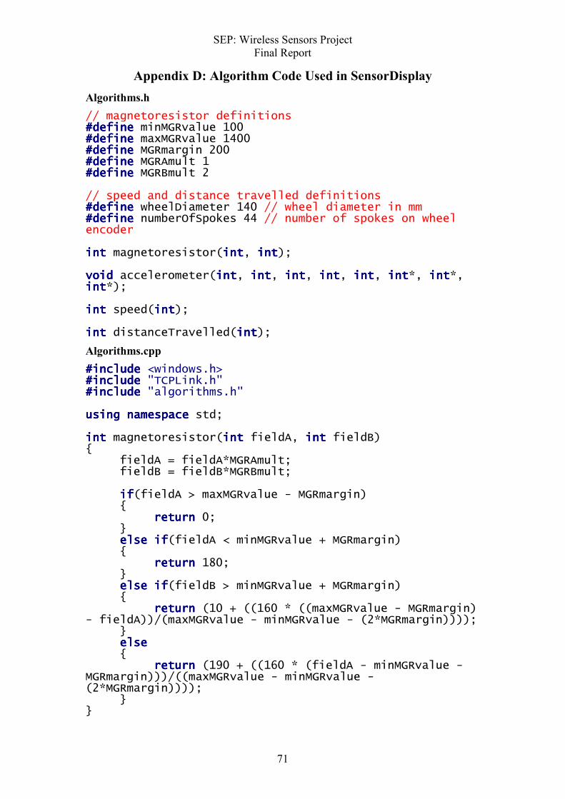
SEP: Wireless Sensors Project Final Report
71
Appendix D: Algorithm Code Used in SensorDisplay
Algorithms.h
// magnetoresistor definitions #define#define#define#define minMGRvalue 100 #define#define#define#define maxMGRvalue 1400 #define#define#define#define MGRmargin 200 #define#define#define#define MGRAmult 1 #define#define#define#define MGRBmult 2 // speed and distance travelled definitions #define#define#define#define wheelDiameter 140 // wheel diameter in mm #define#define#define#define numberOfSpokes 44 // number of spokes on wheel encoder intintintint magnetoresistor(intintintint, intintintint); voidvoidvoidvoid accelerometer(intintintint, intintintint, intintintint, intintintint, intintintint, intintintint*, intintintint*, intintintint*); intintintint speed(intintintint); intintintint distanceTravelled(intintintint);
Algorithms.cpp
#include#include#include#include <windows.h> #include#include#include#include "TCPLink.h" #include#include#include#include "algorithms.h" usingusingusingusing namespacenamespacenamespacenamespace std; intintintint magnetoresistor(intintintint fieldA, intintintint fieldB) { fieldA = fieldA*MGRAmult; fieldB = fieldB*MGRBmult; ifififif(fieldA > maxMGRvalue - MGRmargin) { returnreturnreturnreturn 0; } elseelseelseelse ifififif(fieldA < minMGRvalue + MGRmargin) { returnreturnreturnreturn 180; } elseelseelseelse ifififif(fieldB > minMGRvalue + MGRmargin) { returnreturnreturnreturn (10 + ((160 * ((maxMGRvalue - MGRmargin) - fieldA))/(maxMGRvalue - minMGRvalue - (2*MGRmargin)))); } elseelseelseelse { returnreturnreturnreturn (190 + ((160 * (fieldA - minMGRvalue - MGRmargin)))/((maxMGRvalue - minMGRvalue - (2*MGRmargin)))); } }
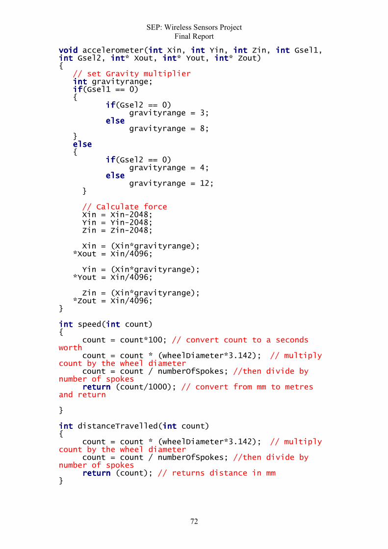
SEP: Wireless Sensors Project Final Report
72
voidvoidvoidvoid accelerometer(intintintint Xin, intintintint Yin, intintintint Zin, intintintint Gsel1, intintintint Gsel2, intintintint* Xout, intintintint* Yout, intintintint* Zout) { // set Gravity multiplier intintintint gravityrange; ifififif(Gsel1 == 0) { ifififif(Gsel2 == 0) gravityrange = 3; elseelseelseelse gravityrange = 8; } elseelseelseelse { ifififif(Gsel2 == 0) gravityrange = 4; elseelseelseelse gravityrange = 12; } // Calculate force Xin = Xin-2048; Yin = Yin-2048; Zin = Zin-2048; Xin = (Xin*gravityrange); *Xout = Xin/4096; Yin = (Xin*gravityrange); *Yout = Xin/4096; Zin = (Xin*gravityrange); *Zout = Xin/4096; } intintintint speed(intintintint count) { count = count*100; // convert count to a seconds worth count = count * (wheelDiameter*3.142); // multiply count by the wheel diameter count = count / numberOfSpokes; //then divide by number of spokes returnreturnreturnreturn (count/1000); // convert from mm to metres and return } intintintint distanceTravelled(intintintint count) { count = count * (wheelDiameter*3.142); // multiply count by the wheel diameter count = count / numberOfSpokes; //then divide by number of spokes returnreturnreturnreturn (count); // returns distance in mm }