Sprint ATL, July 19, 2004 1

Networking Wireless Sensors:New Challenges

Bhaskar KrishnamachariAutonomous Networks Research GroupDepartment of Electrical Engineering-SystemsUSC Viterbi School of Engineeringhttp://ceng.usc.edu/~anrgbkrishna@usc.edu

2

Wireless Sensor Networks

• Large numbers of resource constrained wireless devices, providing a highresolution spatio-temporal interface between the physical and virtual worlds.

• Applications include industrial process monitoring, environmental sensing,ecological studies, military surveillance, structural monitoring, etc.Considerable academic and industry interest in this field in recent years.

• These systems present a number of unique challenges and novel researchproblems that are often fundamentally different from those encountered intraditional networks.

3

Challenges

• Unattended ad-hoc deployment

• Very large scale

• Scarce energy and bandwidth resources

• High noise and fault rates

• Dynamic / uncertain environments

• High variation in application-specific requirements

4

Case Studies

• Phase Transition Phenomena

• Robust, Energy-Efficient Geographic Routing

• Impact of Spatial Data Correlation on Routing with Compression

• Delay Efficient Sleep Scheduling

5

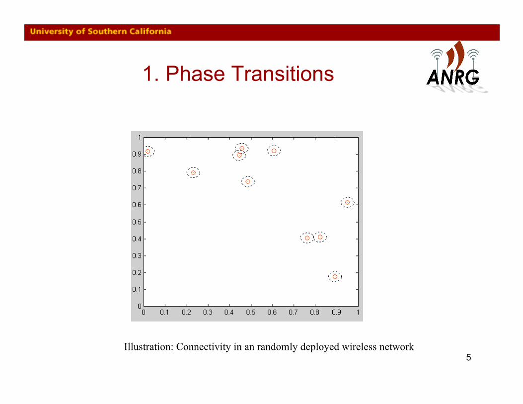
1. Phase Transitions

Illustration: Connectivity in an randomly deployed wireless network

6

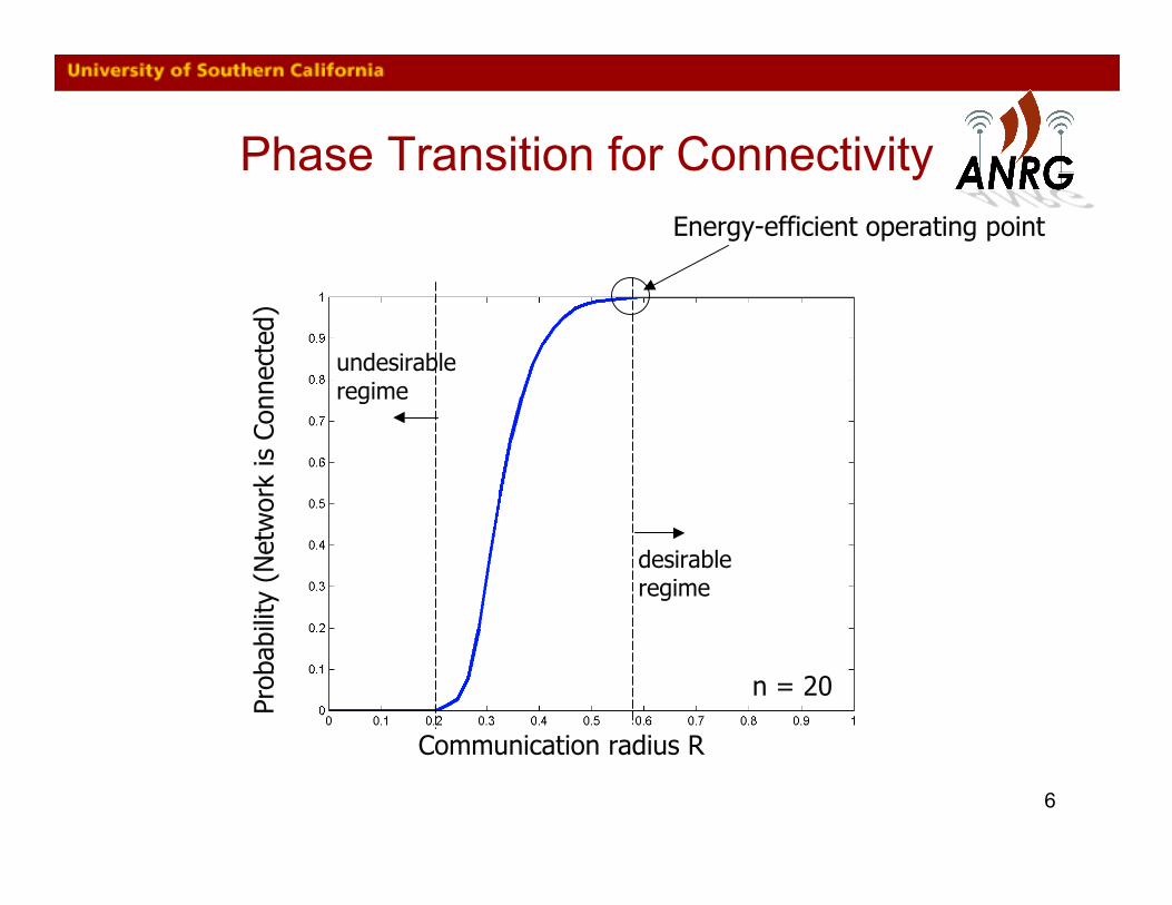
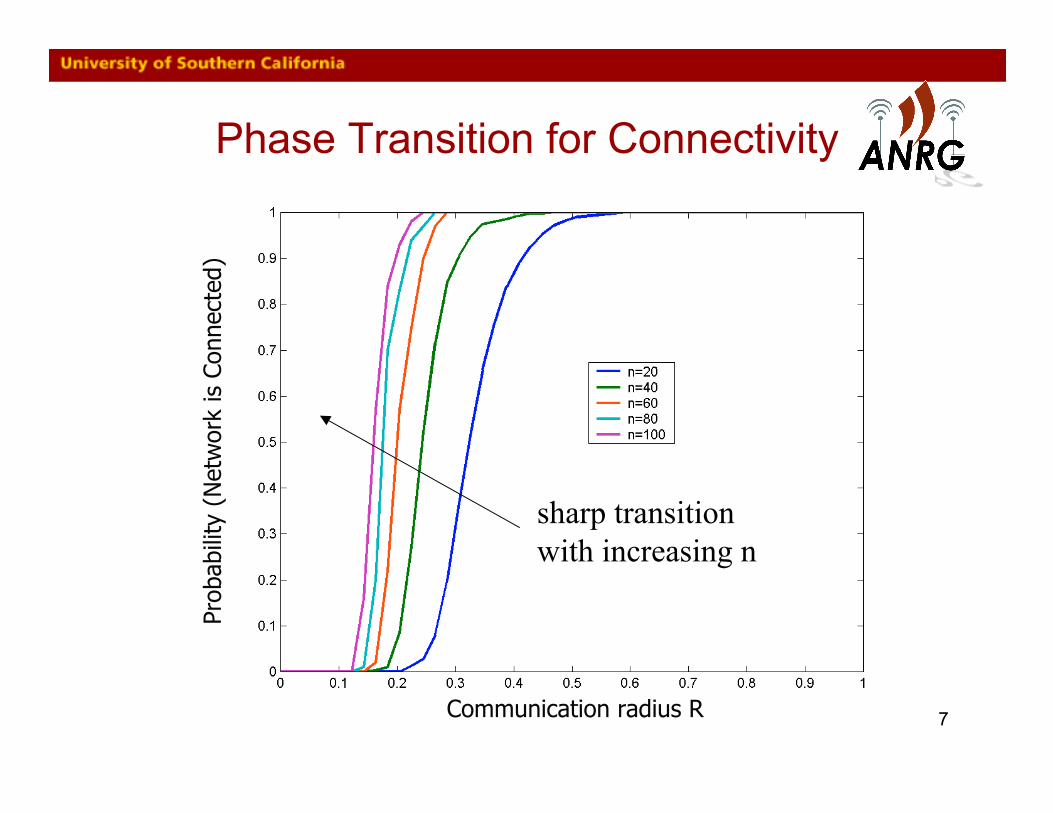
Phase Transition for Connectivity

Prob

abili

ty (

Net

wor

k is

Con

nect

ed)

Communication radius R

Prob

abili

ty (

Net

wor

k is

Con

nect

ed)

undesirableregime

desirableregime

Energy-efficient operating point

n = 20

7

Phase Transition for Connectivity

Communication radius R

Prob

abili

ty (

Net

wor

k is

Con

nect

ed)

sharp transitionwith increasing n

8

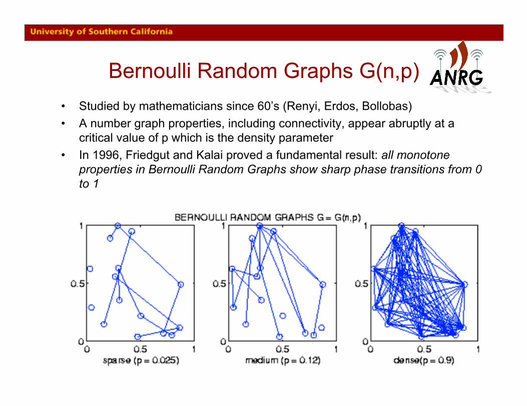
Bernoulli Random Graphs G(n,p)• Studied by mathematicians since 60’s (Renyi, Erdos, Bollobas)• A number graph properties, including connectivity, appear abruptly at a

critical value of p which is the density parameter• In 1996, Friedgut and Kalai proved a fundamental result: all monotone

properties in Bernoulli Random Graphs show sharp phase transitions from 0to 1

9

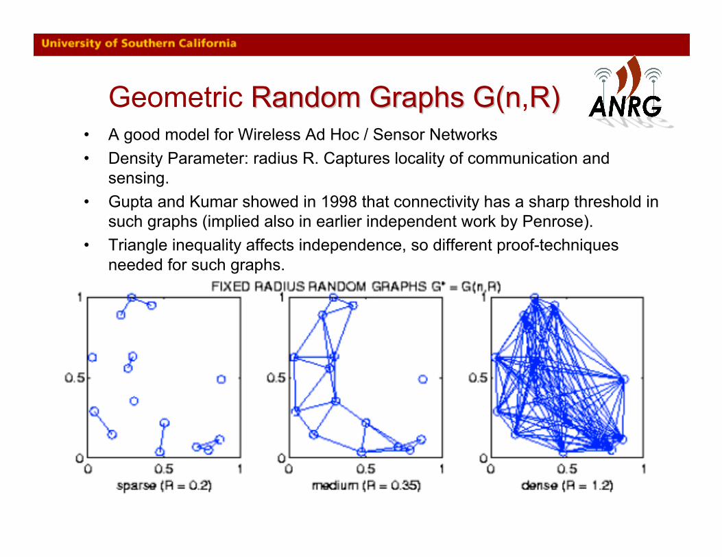
Geometric Random Graphs G(n Random Graphs G(n,R)R)• A good model for Wireless Ad Hoc / Sensor Networks• Density Parameter: radius R. Captures locality of communication and

sensing.• Gupta and Kumar showed in 1998 that connectivity has a sharp threshold in

such graphs (implied also in earlier independent work by Penrose).• Triangle inequality affects independence, so different proof-techniques

needed for such graphs.

10

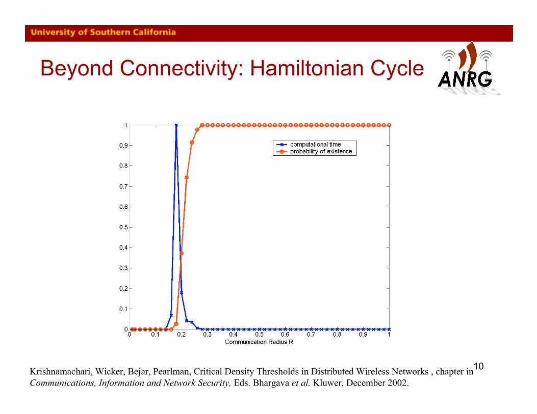
Beyond Connectivity: Hamiltonian Cycle

Krishnamachari, Wicker, Bejar, Pearlman, Critical Density Thresholds in Distributed Wireless Networks , chapter inCommunications, Information and Network Security, Eds. Bhargava et al. Kluwer, December 2002.

11

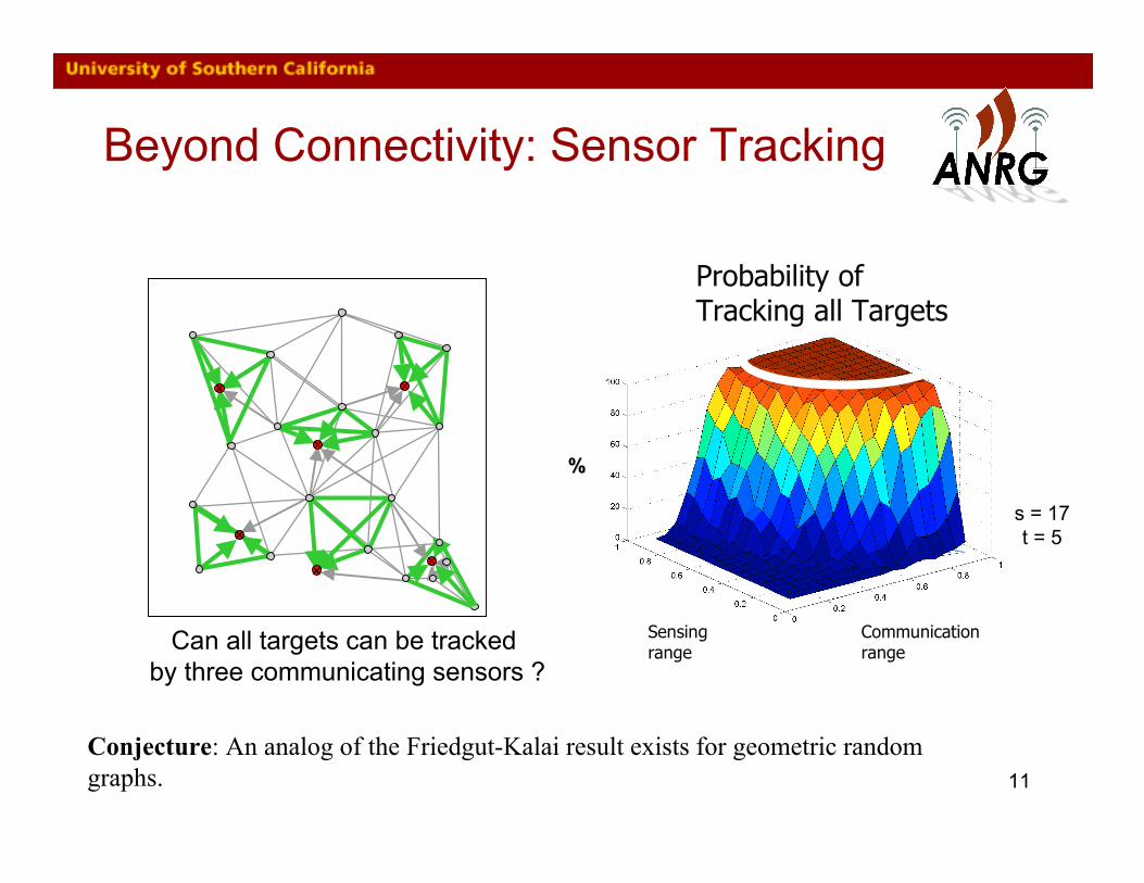
Beyond Connectivity: Sensor Tracking

Can all targets can be tracked by three communicating sensors ?

Probability ofTracking all Targets

Sensingrange

Communicationrange

s = 17t = 5

%%

Conjecture: An analog of the Friedgut-Kalai result exists for geometric randomgraphs.

12

New Result: Sharp thresholds exist forall monotone properties in G(n,R)

• Formally, let the threshold width δ(n, ε) of a property in a geometric randomgraph be the difference in radius between when the property is satisfied withprobability 1-ε and probability ε. The Theorem states that the thresholdwidth of any monotone property δ(n, ε) = o(1) (i.e., asymptotically tends tozero). Specifically, it is proved that δ (n, ε) = O(log3/4n/√n) (for d = 2), andO (log1/dn n-1/d) for d > 2.

• The proof involves the use of bounds on bottleneck matching lengths inrandom geometric graphs. A corollary result shows that a random geometricgraph is a subgraph (w.h.p) of another independently drawn randomgeometric graph with a slightly larger radius.

• Thus, sharp density thresholds exist not only for connectivity but for all othergraph properties of interest in sensor networks - including k-connectivity, k-coloring, Hamiltonian cycles, sensor coverage, etc.

Goel, Rai, Krishnamachari, “Sharp Transitions for Monotone Properties In Random Geometric Graphs,”ACM Symposium on Theory of Computing (STOC), 2004.

13

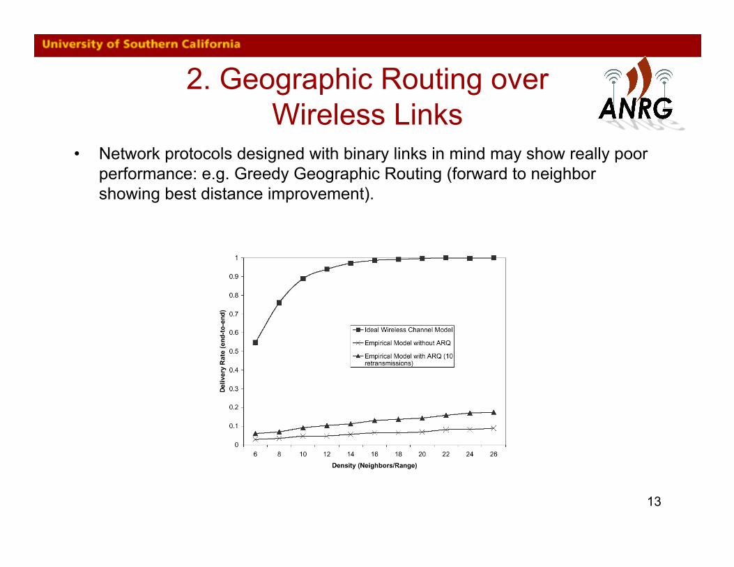
2. Geographic Routing overWireless Links

• Network protocols designed with binary links in mind may show really poorperformance: e.g. Greedy Geographic Routing (forward to neighborshowing best distance improvement).

14

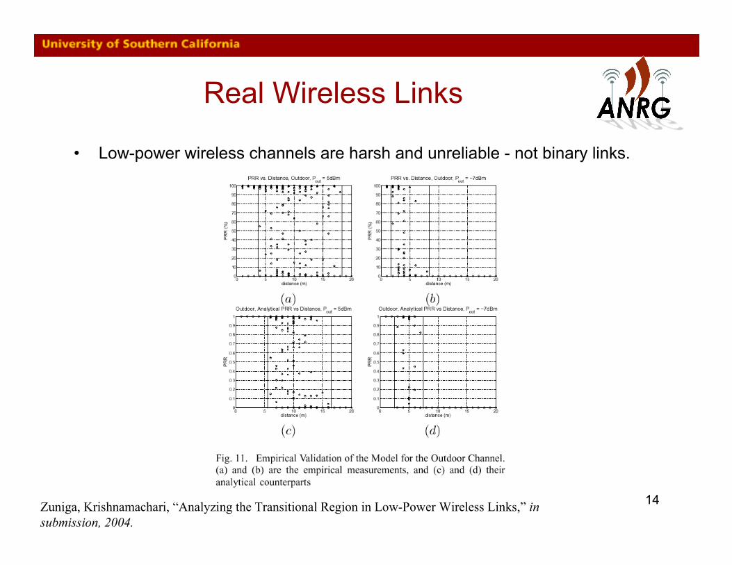
Real Wireless Links

• Low-power wireless channels are harsh and unreliable - not binary links.

Zuniga, Krishnamachari, “Analyzing the Transitional Region in Low-Power Wireless Links,” insubmission, 2004.

15

Two Extremes

1. Forward to best-distance improvement neighbor– Pro: fewer total hops– Con: each long hop likely to have low PRR, hence, may need many retries to get

packet across each hop.

2. Forward to nearby neighbor in direction of destination– Pro: each hop is likely to be high PRR, hence energy-efficient– Con: Requires more total hops, since only a short distance is traveled at each

step

• What’s the right compromise?

16

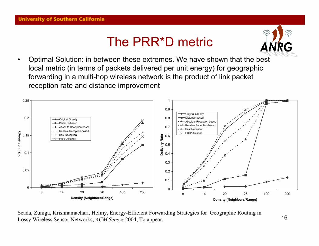
The PRR*D metric• Optimal Solution: in between these extremes. We have shown that the best

local metric (in terms of packets delivered per unit energy) for geographicforwarding in a multi-hop wireless network is the product of link packetreception rate and distance improvement

Seada, Zuniga, Krishnamachari, Helmy, Energy-Efficient Forwarding Strategies for Geographic Routing inLossy Wireless Sensor Networks, ACM Sensys 2004, To appear.

17

3. Impact of Spatial Correlationon Routing with Compression

• Consider a scenario where data is being gathered from a sensor networkmonitoring a physical environment.

• It is now understood that significant energy gains can be obtained bycombining routing with in-network compression, but what is not wellunderstood is the impact of different levels of spatial correlation on jointrouting and compression

• To quantify the energy costs of communication, we use the joint entropy ofn sources to indicate the total amount of compressed information generatedby them.

Pattem, Krishnamachari, Govindan, “Impact of Spatial Correlation on Routing with Compression inWireless Sensor Networks,” ACM/IEEE Symposium on Information Processing in Sensor Networks, IPSN2004. [Best Student Paper Award]

18

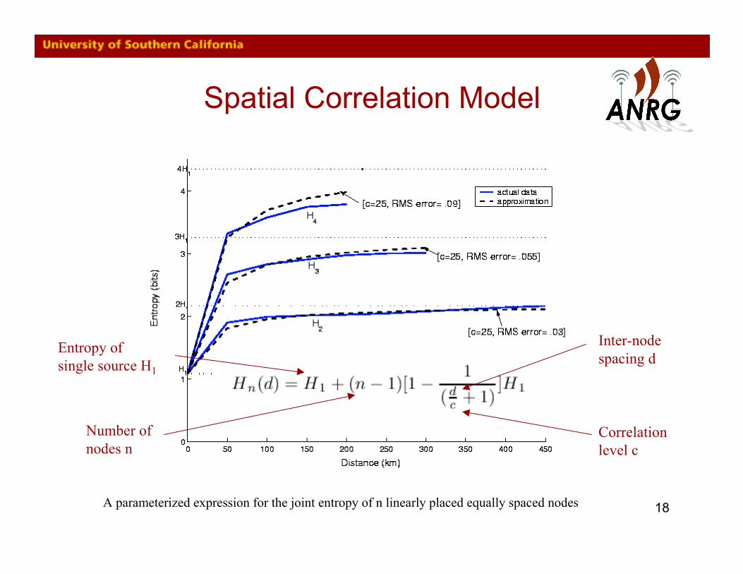
Spatial Correlation Model

Inter-nodespacing d

Correlationlevel c

Number ofnodes n

Entropy of single source H1

A parameterized expression for the joint entropy of n linearly placed equally spaced nodes

19

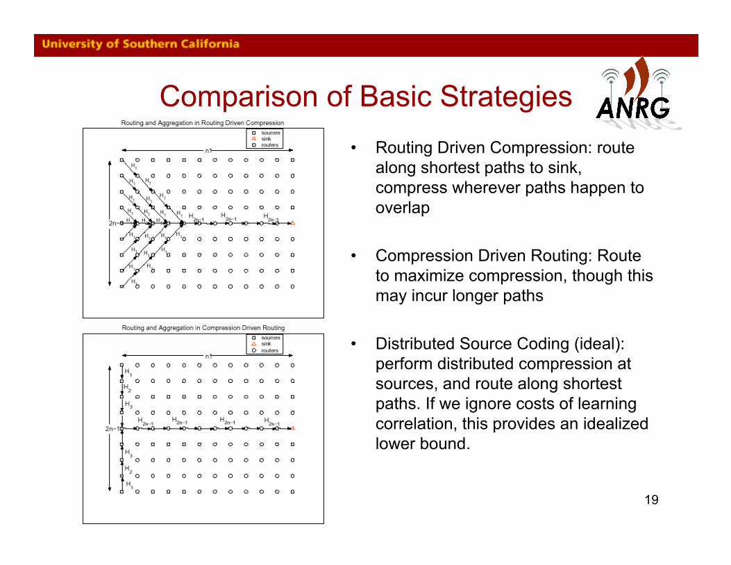
Comparison of Basic Strategies• Routing Driven Compression: route

along shortest paths to sink,compress wherever paths happen tooverlap

• Compression Driven Routing: Routeto maximize compression, though thismay incur longer paths

• Distributed Source Coding (ideal):perform distributed compression atsources, and route along shortestpaths. If we ignore costs of learningcorrelation, this provides an idealizedlower bound.

20

Comparison of Basic Strategies

21

Generalizing the strategies

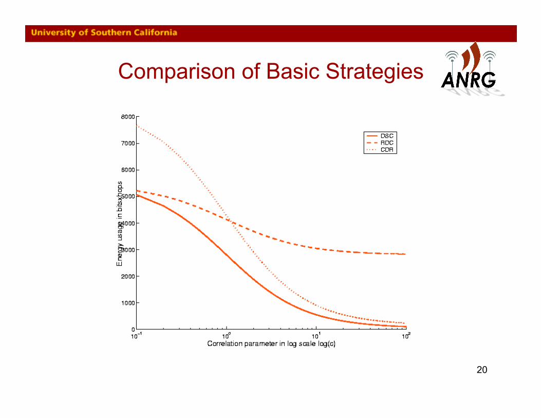
• We find that a CDR strategy works well with high correlation, and an RDCstrategy works best at low correlation -- what about in between?

• We can look for some hybrid techniques, but there must be somesystematic way to parameterize them, if we are to have any hope ofanalysis.

• Solution: Clustering. Create clusters of nearby sources. First route tocompress the data within the sources inside each cluster, then route thecompressed data from the clusters towards the sink along shortest pathsand compress further where there is overlap. RDC and CDR are then thetwo extreme special cases (cluster of 1 source, and cluster of n sources).

22

Analysis

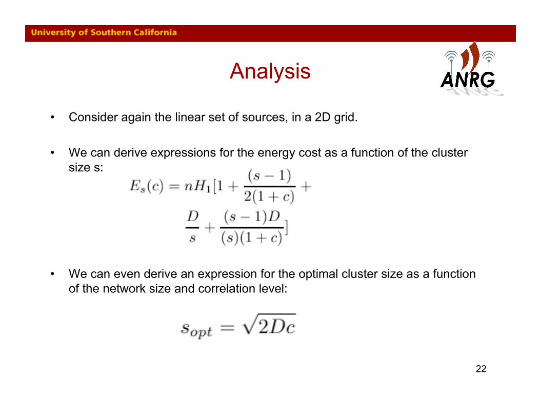
• Consider again the linear set of sources, in a 2D grid.

• We can derive expressions for the energy cost as a function of the clustersize s:

• We can even derive an expression for the optimal cluster size as a functionof the network size and correlation level:

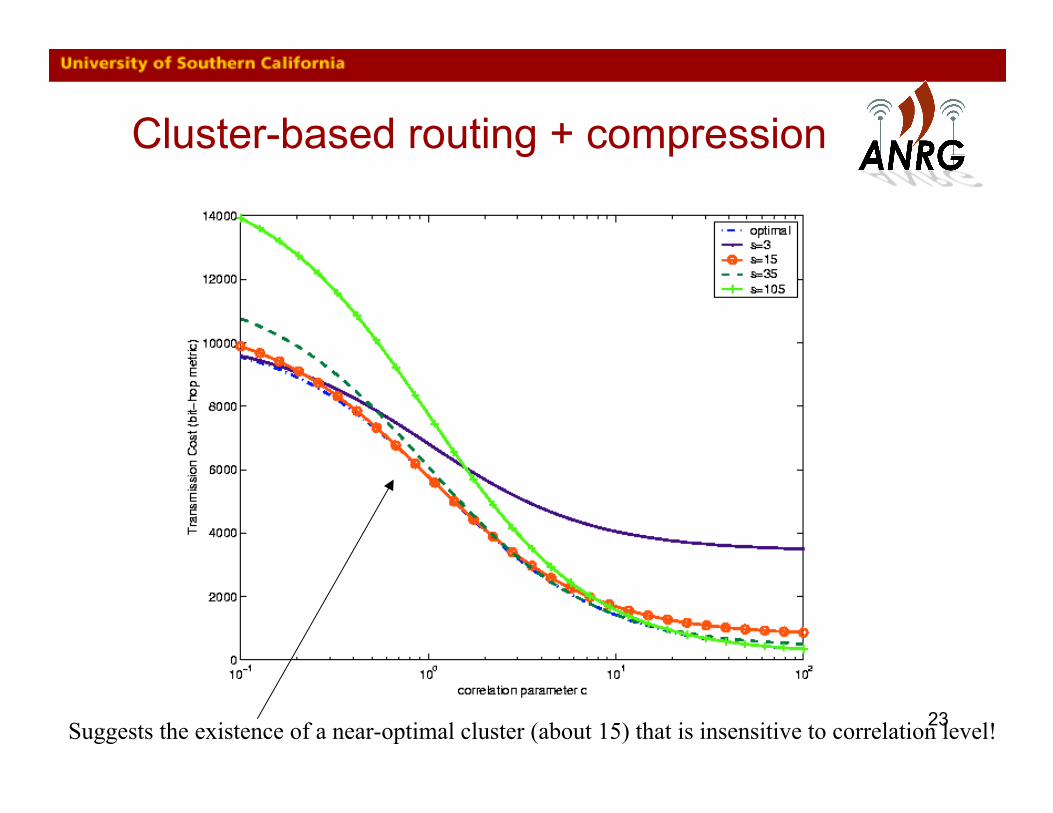
23

Cluster-based routing + compression

Suggests the existence of a near-optimal cluster (about 15) that is insensitive to correlation level!

24

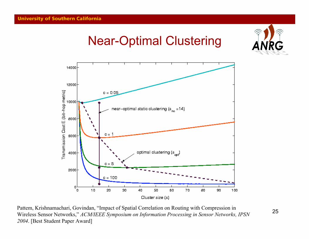
Near-Optimal Clustering

• Can formalize the notion of near-optimality using a maximum differencemetric:

• We can then derive an expression for the near-optimal cluster size:

• This is independent of the correlation level, but does depend on the networksize, number of sources, and location of the sink. For the above scenario, itturns out sno = 14 (which explains the results shown).

25

Near-Optimal Clustering

Pattem, Krishnamachari, Govindan, “Impact of Spatial Correlation on Routing with Compression inWireless Sensor Networks,” ACM/IEEE Symposium on Information Processing in Sensor Networks, IPSN2004. [Best Student Paper Award]

26

4. Delay-Efficient Sleep Scheduling

• Largest source of energy consumption is keeping the radio on (even if idle).Particularly wasteful in low-data-rate applications.

• Solution: regular duty-cycled sleep-wakeup cycles.

• Say there are k slots, each node stays awake for one of these slots toreceive packets intend for it. It makes this cycle known to its neighbors sothey know when to wake up and transmit a packet to it.

• While this limits energy consumption, it can introduce significant sleep delay.E.g. if all nodes synchronize to wake and sleep at the same time, then apacket will take m cycles (m*k slots) to traverse m hops in the network.

27

Illustration

28

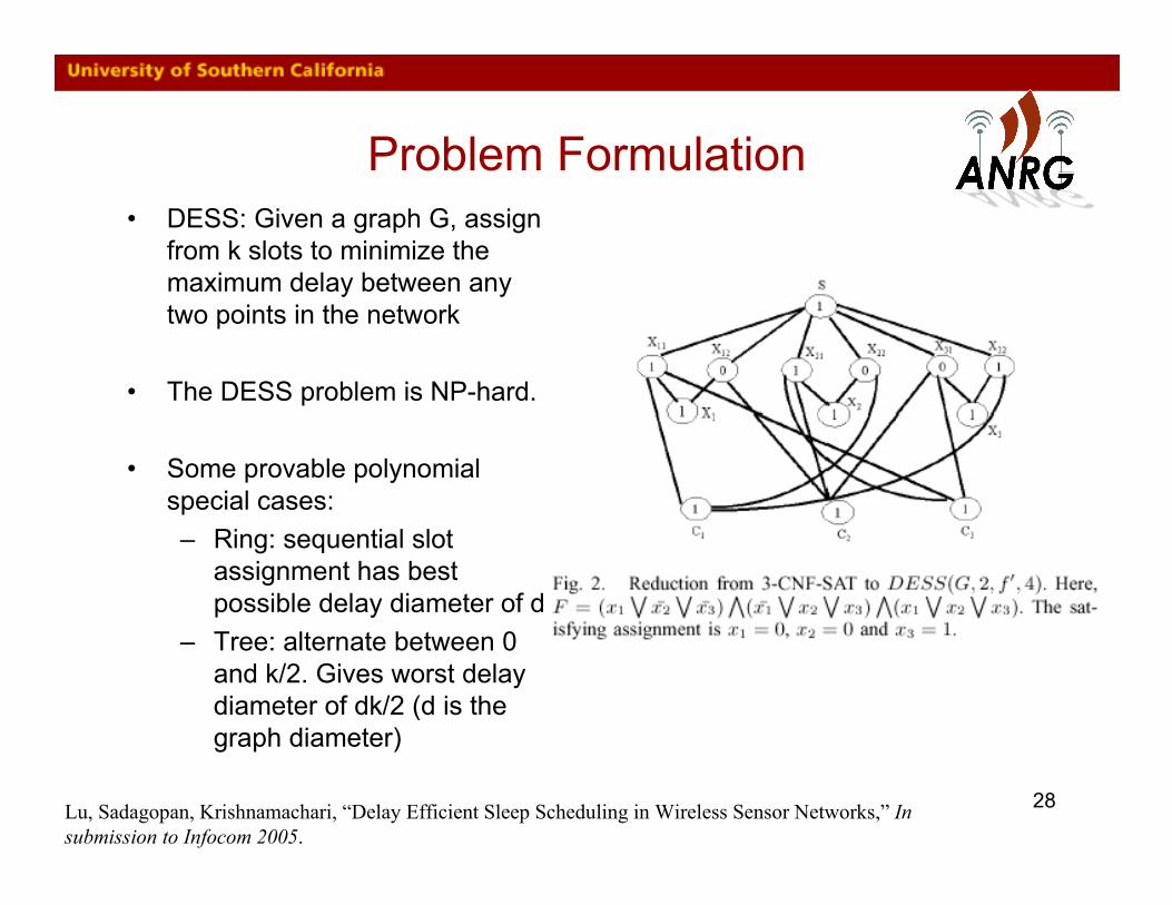
Problem Formulation• DESS: Given a graph G, assign

from k slots to minimize themaximum delay between anytwo points in the network

• The DESS problem is NP-hard.

• Some provable polynomialspecial cases:– Ring: sequential slot

assignment has bestpossible delay diameter of d

– Tree: alternate between 0and k/2. Gives worst delaydiameter of dk/2 (d is thegraph diameter)

– hLu, Sadagopan, Krishnamachari, “Delay Efficient Sleep Scheduling in Wireless Sensor Networks,” Insubmission to Infocom 2005.

29

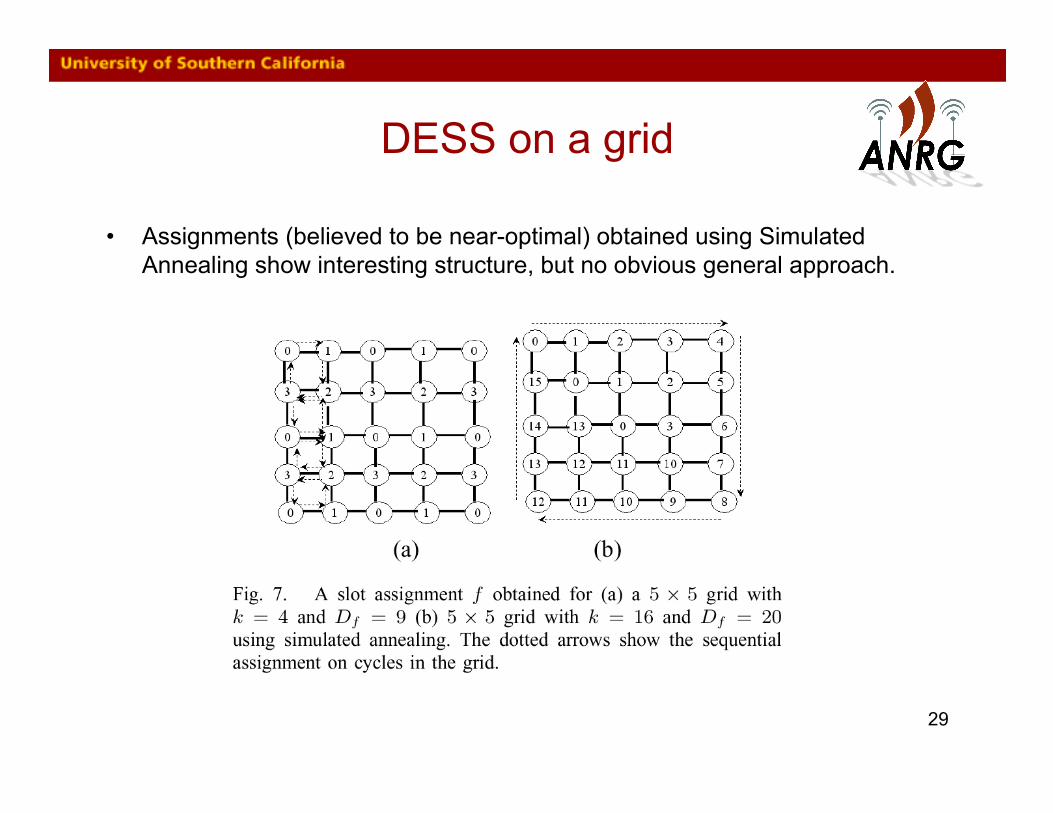
DESS on a grid

• Assignments (believed to be near-optimal) obtained using SimulatedAnnealing show interesting structure, but no obvious general approach.

30

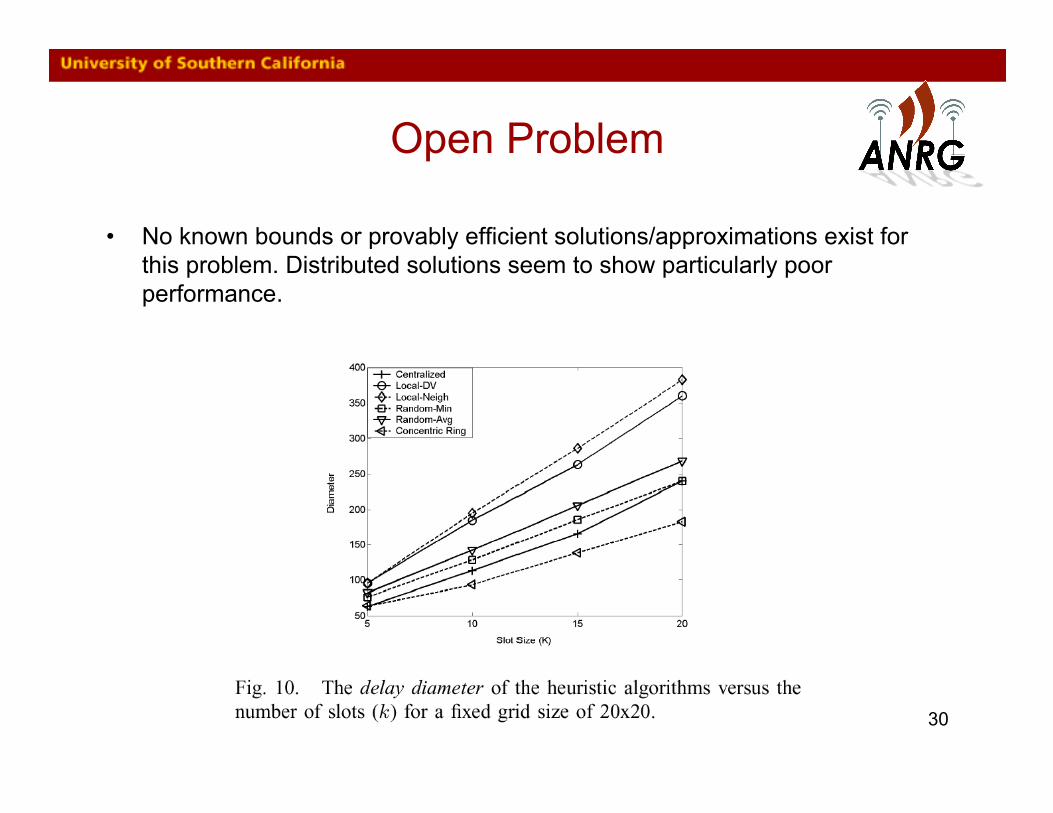
Open Problem

• No known bounds or provably efficient solutions/approximations exist forthis problem. Distributed solutions seem to show particularly poorperformance.

31

Summary

• We examined a number of interesting case studies– existence of phase transitions in geometric random graphs,– existence of near-optimal routing+compression structures,– metric for efficient geo-routing in the face of unreliable links– delay efficient radio sleep schedules

• They show the novelty and richness of the design and analytical challengesinvolved in networking wireless sensors.

32

Sequential Pagingin Cellular Wireless Networks

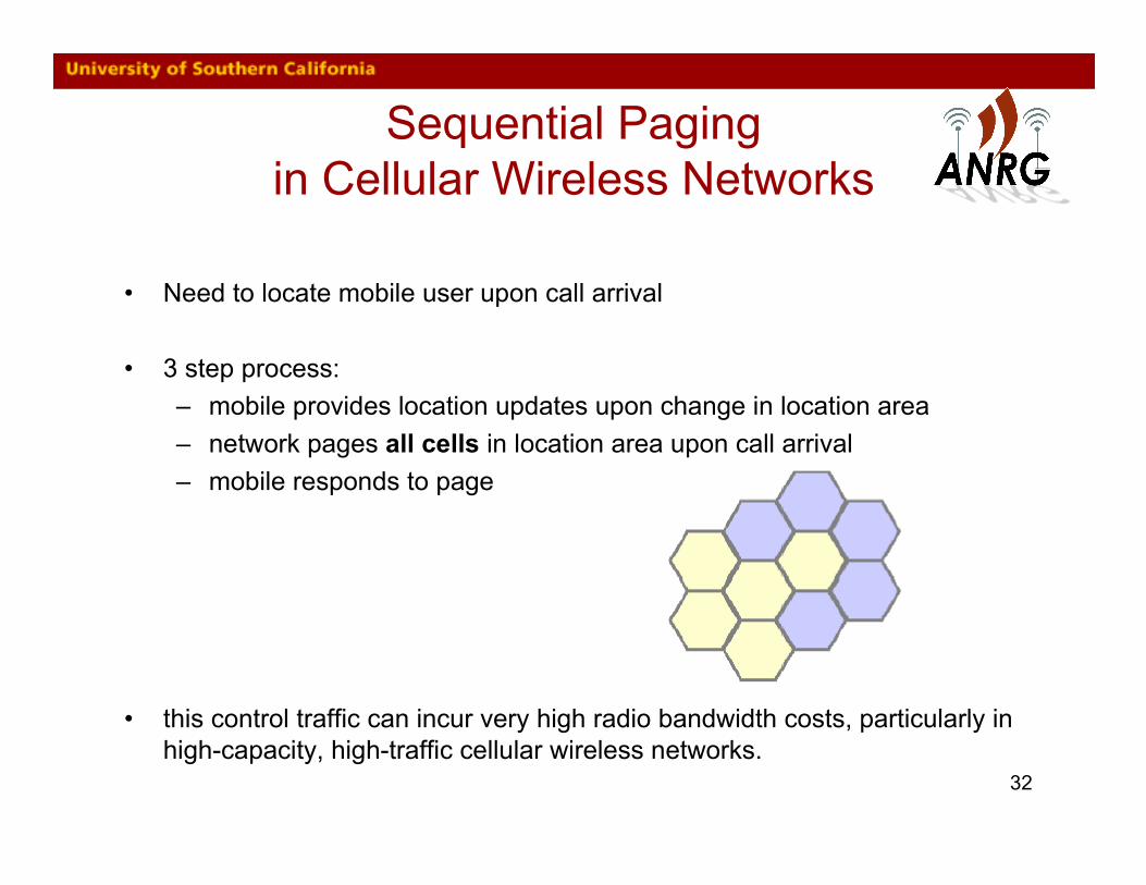
• Need to locate mobile user upon call arrival

• 3 step process:– mobile provides location updates upon change in location area– network pages all cells in location area upon call arrival– mobile responds to page

• this control traffic can incur very high radio bandwidth costs, particularly inhigh-capacity, high-traffic cellular wireless networks.

33

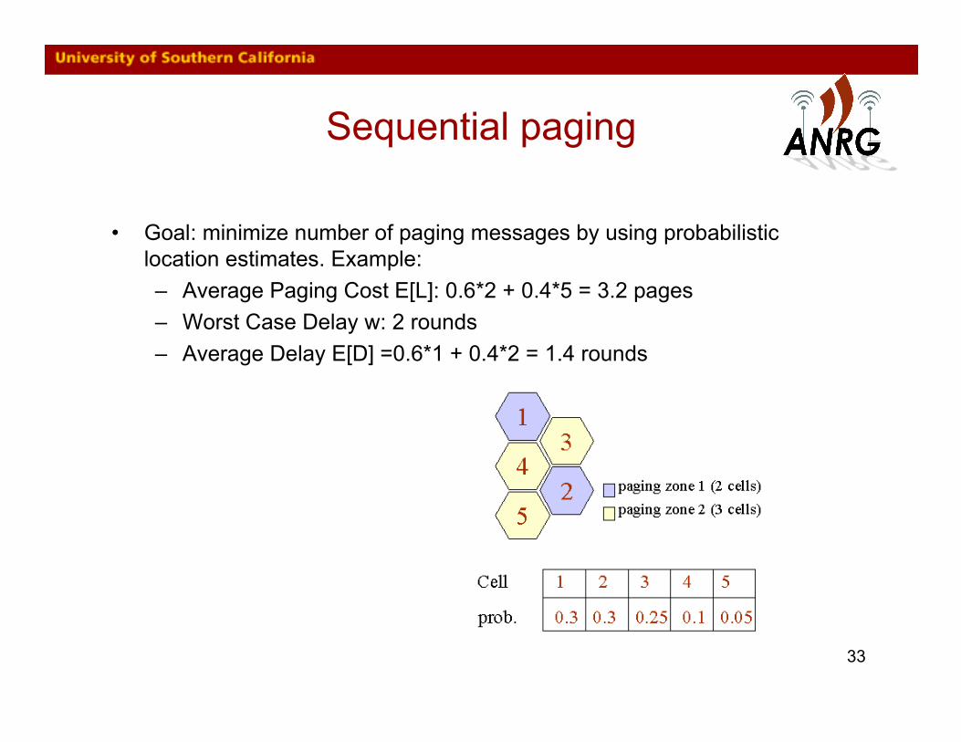
Sequential paging

• Goal: minimize number of paging messages by using probabilisticlocation estimates. Example:– Average Paging Cost E[L]: 0.6*2 + 0.4*5 = 3.2 pages– Worst Case Delay w: 2 rounds– Average Delay E[D] =0.6*1 + 0.4*2 = 1.4 rounds

34

Results• Problem of minimizing average paging cost subject to a constraint on the

average delay was believed to be intractable:• “This problem is not amenable to solution via Dynamic

Programming owing to the constraint on E[D]” - Rose & Yates 1995.• “(This Problem) is NP-complete” - Abutaleb & Li, 1997

• We developed an O(n3) dynamic programming solution to this problem,proving its tractability.

• Also derived analytical results quantifying the performance of sequentialpaging, showing that very high gains are possible when the user locationprobabilities are concentrated within a small subset of the full region.

• Open Question: how can these probabilities be estimated in practice?

Krishnamachari, Gau, Wicker, Haas, “Optimal Sequential Paging in Cellular Networks,” ACM Wireless Networks,March 2004.

35

Integrating Cellular & Sensor Networks

• Compelling reasons to look at the intersection of these two domains, sincecellular networks represent an already-existing large-scale wireless system

• Questions:– Can the cellular network itself be treated as a sensor network, by

equipping cellular devices with sensing capabilities?– Can the cellular network infrastructure be leveraged to extract data from

large scale pervasive sensor systems (e.g. by designing mechanisms toroute to random, mobile sinks)?

• These questions are being pursued already in commercial settings, notablyin the Pervasive Indeterminate Measurement Systems (PIMS) work byresearchers at Agilent (J. Warrior, J. Eidson et al.).