Final Report on

MARGINAL COST RATEMAKING FOR COGENERATION, INrERRUPI'IBLE, AND BACK-UP SERVICE S

Roger McElroy Timothy Pryor

Russell Profozich Amy Garant

Kaye Pfister

THE NATIONAL REGULATORY RESEARCH INSTITUTE 2130 Neil Avenue

Columbus, Ohio 43210

prepared for the

U.S. Department of Energy Economic Regulatory Administration Division of Regulatory Assistance

in partial fulfillment of

Grant No. DE-FG01-80RG10268

February 1981

This report was prepared by The National Regulatory Research Institute under a grant from the U.S. Department of Energy (DOE). The views and opinions of the authors do not necessarily state or reflect the views, opinions, or policies of OOE, or The National Regulatory Research Institute.

Reference to trade names or specific commercial products, commodities, or services in this report does not represent or constitute an endorsement, recommendation, or favoring by DOE or The National Regulatory Research Institute of the specific commercial product, commodity, or service.

EXECUTIVE SUMMARY

Recent developments in federal law and regulatory rulings have required state public utility commissions (PUCs) to re-examine the electric pricing policies and rate structures of electric utilitiese Among other requirements, PUCs must consider the appropriateness of pricing electricity on the basis of its marginal cost. This report explores the application of marginal cost pricing principles to three special electric ratemaking areas: cogeneration rates, interruptible rates, and the setting of rates for back-up power.

With respect to cogeneration purchases, FERC rules generally require that rates equal the utility's avoided cost. Calculation of avoided cost is equivalent to calculation of some type of utility marginal cost. The relevant marginal cost depends on whether the utility avoids energy costs only or avoids additional capacity costs as well.

Two classes of interruptible service are here proposed, one with a minimum,target reliability (Class I) and the other without (Class II). The objective is to avoid the extremes of either subsidizing nominally inter­ruptible customers who in practice are rarely interrupted or requiring all interruptible customers to accept a high frequency and extent of inter­ruption. The Class I interruptible rate includes a demand charge to reflect the marginal costs of the generation, transmission, and distri­bution capacity required to maintain service at a target level ofrelia­bility. Class II interruptible service, which has no minimum reliability specification, is provided only when utility capacity is available and thus has no demand charge included in its rate.

Various forms of back-up power service are defined and their marginal costs of service discussed. The lack of information on the load demands of back-up customers will, much of the time, make the creation of a sepa­rate cost-based rate class for these customers difficult. Where the number of customers is small and their load demands uncertain, including back-up customers in regular rate classes or adopting an experimental rate with interruptible (or off-peak) provisions may be a commission's most prudent short-run course of action until more is known about the characteristics of potential back-up subscribers.

iii

ACKNO~Jlli DGHE NT S

The authors are indebted to a number of persons at The National Regulatory Research Institute who made significant contributions to this report. First among these is Dr. Kevin A. Kelly, Associate Director for Electric and Gas Research. His overall direction of the project and his many suggestions and criticisms of earlier drafts of the report improved both the substance and style of the final product. Dr. Daniel Z. Czamanski, Institute Fellow in Economics, also read these drafts and his challenges forced us on many occasions to sharpen our economic thinking. In addition, Drs. Douglas N. Jones and Raymond 'J. Lawton, Director and Associate Director, respectively, offered a number of suggestions on an earlier draft that improved the quality of the final version. In the early stages of the study, Karen Riccio labored evenings and weekends to trans­form our initial scribblings into a typewritten first draft. Finally, Lynne Berry displayed uncommon professionalism and restraint, suffering with us through months of revisions to produce the final typed copy.

While these people helped us to avoid many errors and omissions during the course of the study, they should in no way be held accountable for those that remain.

iv

TABLE OF CONl'ENTS

Chapter Page

1

2

3

INTRODUCTION

Background •• e 0 e eo. • • • • 0 • • • • • •

Current Controversies in Electric Utility Pricing • Basic Principles of Marginal Cost Pricing G

Organization of the Report • & • • • • • •

PART I" MARGINAL CO ST 'RATEMAKING FOR POWER PURCHASE S FROM COGENERATION AND SMALL POWER PRODUCTION FACILITIE S

INl'RODUCTION TO COGENERATION RATEMAKING

Cogeneration ". • • • • •• • • • • • • • Cogeneration from the Utility and

Industrial Perspectives • • Federal Action on Cogeneration G e 8 • •

Some Issues in Setting Cogeneration Rates

METHODS FOR COMPUTING MARGINAL COST BASED ESTIMATES OF lfrILITY AVOIDED COSTS AND CONVERTING THESE COSTS I NTO RATE See G tilt 0 e e ., e e tit .. • • • • .. • " •

1

2 4 5 7

11

11

12 15 17

21

Marginal Costs and Avoided Costs: How Are They Related? •• 8 22 The Structure of Utility Costs: What Costs Can Be Avoided

as a Result of Purchases from Cogenerators? •••••• "e 25 Marginal Cost Based Methods for Computing Utility

Avoided Costs • • " • • 0 • • • 0 G •

Rates Based on Avoided Costs • • • •

PART 11., MARGINAL CO 8T RATEMAKING FOR INl'ERRUPTIBLE SERVICE

27 41

4 INTRODUCTION TO INTERRUPrIBLE SERVICE RATEMAKING 47

Electricity and Product Differentiation Value-Based versus Cost-Based Pricing

of Interruptible Service •. • • •• ..".. Load Management, Capacity Planning, and the

Reliability of Interruptible Service The Economics of System Reliability and

Interruptible Electric Service Recent State Public Utility Commission Rulings The Perspective of Industrial Consumers e • • • •

v

48

49

50

52 56

o e .. • 58

TABLE OF CONTENTS (Continued)

Chapter Page

5 METHODS FOR COMPUTING THE MARGINAL COST OF INTERRUPTIBLE SERVICE AND CONVERTING THESE COSTS INTO RATES •••••

Capacity Planning, Service Reliability, and

59

Interruptible Service • 60 Calculating Marginal Cost Based Rates for Class I and Class II

Interruptible Service • • • • • • • • • • • • 64 Potential Problems and Limitations in Implementing a

Marginal Cost Based Interruptible Rate 76

PART III. MARGINAL COST RATEMAKING FOR BACK-UP SERVICES

6 INTRODUCTION TO RATEMAKING FOR BACK-UP SERVICES · . . . 89

7

Definitions of Back-Up Services • • • • • • • • Soole Issues in Ratemaking for Back-Up Services Department of Energy Voluntary Guideline • • • • Experimental Rates by State Public Utility Commissions

· . . . · . . .

90 92 94 96

METHODS FOR COMPurING THE MARGINAL COSTS OF AND RATES FOR INTERRUPTIBLE SERVICE • • • • • •• 101

Types of Back-Up Service Demand and Problems in Determining their Impacts on Utility Cost of Service • • • • •• 101

Methods for Computing the Marginal Costs of and Marginal Cost Based Rates for Back-Up Services •• • • •••• • • • • 105

WORKS CITED 113

vi

CHAPTER 1

INTRODUCTION

In this report, methods are developed for calculating marginal cost

based rates in three special electric tariff situations: the purchase of

electricity from cogenerators and the sale of interruptible and back-up

power. These methods are intended to assist state public utility com­

missions in evaluating the applicability of marginal cost pricing prin­

ciples to the solution of these special ratemaking problems. As such, this

report should be viewed as an attempt to fill a current void in the infor­

mational and analytical resources available to state commissions.

Power supplied to utilities by cogenerators can be delivered on a firm

basis or on an as-available basis. Costing and pricing methods are

presented for both types of deliveries. The methods presented apply

equally to ratesetting for utility purchases from cogeneration and small

power production facilities qualifying for the special ratemaking

provisions of the Public Utility Regulatory Policies Act of 1978 (PURPA),

Section 210. For the sake of brevity and convenience, the word cogen­

eration (and its variations) will be used generally to refer to ratemaking

for both types of qualifying facilities. Interruptible service is that

supplied to a customer with a provision that allows the utility to

interrupt the customer's power supply for short periods, usually during

times of extreme peak demand or other system emergency conditions. Back-up

service can take any of three forms: supplementary power, maintenance

power, and stand-by power. Supplementary power is that sold to a customer

to make up the difference between his needs and what he can regularly

generate himself. Maintenance power is that provided to a customer during

scheduled outages of his facility. Stand-by service is defined as that

provided to customers during unscheduled outages of their primary systems.

1

Background

The decade of the 1970s brought dramatic changes in the political

economies of energy production and consumption in the United States. The

ten-fold increase in the price of imported oil and the growing uncertainty

about its continued availability (at any price) have led the list of

reasons for national re-examination of energy policies. One area that has

received a large share of policymaking attention in this re-examination

process is the regulation of electric utilities.

Rapidly rising fuel costs, together with escalation in the cost of

capital equipment and labor, have resulted in substantial increases in the

cost of electric energy for most consumers. The upward surge has been par­

ticularly noticeable since, for many years, the economies associated with

realization of large-scale production allowed electricity's price per kilo­

watt-hour to fall at the same time that the prices of most other goods were

rising. Developments of the 1970s reversed this downward trend and caused

public utility commissions to become increasingly interested in mechanisms

for combatting the steady rise in electricity prices.

As the cost of electricity has risen, so have concerns about the

equitable recovery of this cost from utilities' ratepayers. Possible

subsidies of one class or category of users by another received less

attention when electric costs were declinin~. However, as the size of

customers' electric bills has risen, so have the pressures for more

equitable ratemaking.

Higher costs also have called attention to two other aspects of

utility operations: efficiency and energy conservation.. Efficiency in the

electric utility industry has two distinct but related elements: its

engineering and economic aspects. In the engineering sense, efficiency

generally refers to the process of achieving high productivity, so that a

maximum amount of electricity is generated from a given amount of fuel and

a fixed amount of investment in plants and equipment. This often means

2

minimizing the amount of time a base load plant is idle or not fully

productive. Economic efficiency, on the other hand, requires the

allocation of scarce, energy-producing resources in such a way that results

in output being produced only for those purposes justified by the cost, and

not for economically wasteful purposes. Conservation depends on the

elimination of inefficiency and waste in both production and consumption of

electric energy.

Many of the problems relating to customer cross-subsidization, improv­

ing utility efficiency, and conserving scarce resources have been caused by

the faster growth of utility peak demand (when both costs and scarce fuel

consumption are greatest) relative to off-peak demand (when both are

lowest). Many regulatory reforms, therefore, have been aimed at altering

this trend in growth of peak demand, or at least softening the negative

impacts of that part of it which cannot be altered.

In this regard, PURPA Section 101 supplements otherwise applicable

state laws to establish conservation, efficiency, and equity as purposes of

utility regulation. Its provisions require state utility commissions to

adopt or consider adopting measures oriented toward achievement of these

purposes. Section III of PURPA is also notable in that it establishes six

ratemaking standards for state commissions to consider as tools for

achieving these regulatory goals. The six standards are:

1) basing all rates on cost-of-service for the utility;

2) eliminating declining block-rate structures in electric rate-

making;

3) establishing time-of-day rates in electric ratemaking;

4) establishing seasonal rates for electric consumption;

5) requiring utilities to offer interruptible rates; and

6) requiring utilities to offer appropriate load management tech­

niques to their customers.

3

Furthermore and especially relevant to the purpose of this report,

Section 131 of PURPA authorizes the Secretary of the U.S. Department of

Energy (DOE) to prescribe voluntary guidelines for state commissions to use

in their consideration of these PURPA ratemaking standards. In its

proposed Voluntary Guideline Number 4, the DOE has recommended that

marginal cost principles be used in implementing the cost-of-service

standard. 1

Current Controversies in Electric Utility Pricing

One of the most familiar current debates in public utility regulation

is over the proper method for analyzing costs for the purpose of pricing a

utility's output. 2 Nowhere is this controversy more focused than in

electricity pricing. The debate centers primarily upon what should be

considered the "true cost" of providing electric service, especially for

purposes of constructing equitable rates and providing correct price

signals to consumers. Antagonists align themselves either with the more

traditional and often more familiar average cost approach (also commonly

referred to as embedded cost, historic cost, accounting cost, or fully

distributed cost method) or the non-traditional and often less well

understood marginal cost approach. Since the general issues, implications,

and problematic concerns associated with each approach are widely discussed

in the literature,3 no attempt will be made to recapitulate or advance the

discussion here. Nor does this report or its authors advocate or seek the

1Federal Register, Vol. 45, No. 173, September 4, 1980, pp. 58767-68.

2For an erudite and comprehensive but plainly worded introduction to the economics of public utility pricing, see Edward E. Zajac, Fairness or Efficiency: An Introduction to Public Utility Pricing (Cambridge, Mass.: Ballinger Publishing Company, 1978.)

3For those not already familiar with traditional electric costing and pricing methodologies, see for example, James C. Bonbright, Principles of Public Utility Rates (New York: Columbia University Press, 1961); and John J. Doran, et al., Electric Utility Cost Allocation Manual (Washington, D.C.: National Association of Regulatory Utility Commissioners, 1973). For

4

adoption of one or another of the approaches by ratemaking authorities.

Rather, it seeks to help fill what appears to be an information void in the

regulatory community: methods for applying marginal cost pricing principles

in special electric tariff situations. In particular, how does one go

about developing and considering a marginal cost based rate for cogener­

ation purchases, interruptible service, and back-up services?4

Basic Principles of Marginal Cost Pricing

For years economists have noted the benefits of marginal cost based

prices and have advocated their use. Not until fairly recently, however,

has the concept of marginal cost pricing received widespread attention in

electric utility ratesetting in the United States. Economic theory states

that maximum economic benefits to society can be achieved if prices are set

equal to marginal costs. Marginal cost is the cost of producing one addi­

tional unit of an industry's output, other things remaining the same. If

the price of all units sold is set equal to the marginal cost, the customer

will pay an amount that adequately reflects the cost to society of

producing the product. In this way, economic efficiency is achieved in

that society's scarce resources are used in productive processes where the

prices of finished goods and services adequately reflect the actual costs

of producing them.

overviews of marginal cost pricing as it pertains to the electric utility industry, see Alfred E. Kahn, The Economics of Regulation, vol. I (New York: John Wiley & Sons, Inc., 1975); Edward E. Zajac, Ope cit.; and Daniel Z. Czamanski, J. Stephen Henderson, Kevin A. Kelly, et ale, Electric Pricing Policies for Ohio, 2 volse, NRRI-77-1 (Columbus: The National Regulatory Research Institute, 1977). For a comparative discussion of average vs .. marginal cost: approaches, see Kevin A. Kelly, et al .. , "An Outline Discussion of the PURPA Ratemaking Standards," Columbus, Ohio, September 1980 ..

4The need for assistance in these ratemaking areas was initially identified in a roundtable meeting conducted by the NRRI of state utility commissioners and senior staff in attendance at the Annual Meeting of the National Association of Regulatory Utility Commissioners in Atlanta, Georgia on December 5, 1979.

5

The cost of producing electricity varies by time of day, day of the

week, and season of the year. This pattern results primarily from the fact

that load demands placed on the utility's generating system vary signifi­

cantly along these time dimensions. This creates a series of peak and

off-peak demand periods, each with its own optimum mix of generating plant

types best suited to meet it. Since these optimum configurations have

different capital and operating expense requirements associated with them,

total and average production expenses vary accordingly. For the same

reasons, the marginal cost of meeting an electric load increment (or

decrement) also varies.

Economists believe that electric rates based on variable marginal

costs send the correct price signals to consumers. Only by setting

electric rates as closely as possible to the utility's marginal production

costs, economists say, can regulators communicate to consumers the actual

cost consequences of expanded consumption and thus enable prices to serve

the interests of economic efficiency. Other analysts question the validity

of the economists' notion of economic efficiency, particularly as it

applies to the regulated sectors of the economy. The primary purpose of

rate regulation, as these analysts see it, is to ensure that prices are

fair and not necessarily to influence the consumption behavior of

ratepayers. Regulators should be concerned that rates are fair to the

utility: they should result in revenue adequate to cover the company's

operating expenses and to provide a fair return to investors. Rates must

also be fair to consumers: they must not be higher than necessary to cover

legitimate company costs, and they should sufficiently differentiate among

customer classes according to the costs each imposes on the utility system.

From these analysts' viewpoint, pricing electricity on the basis of average

costs achieves a rate that satisfies these criteria.

The most familiar aspects of marginal cost based electric ratemaking

are time-of-day (TOD) and seasonal pricing,S but there are other potential

STOD and seasonal rates also can be calculated on the basis of aver-

6

areas for its application. While this report will not seek to resolve the

theoretical issues separating marginal cost from average cost pricing

advocates, it will explore some of the less familiar areas of electric

marginal cost pricing applications. Since most electric rates in the

United States are hased on one or another variation of average cost

pricing, its ratemaking implications are fairly well known. Marginal cost

pricing applications to electric ratemaking, on the other hand, are

relatively new. Despite two years of intense debate, their implications

for electric ratemaking still are not fully understood by all regulators or

members of the utility industry. The rulings of the U.S. DOE and the

Federal Energy Regulatory Commission clearly imply that marginal cost

principles should be considered in the PURPA process. Lastly, rates for

purchases from cogenerators (Section 210), interruptible rates (Section 111

and 210), and back-up rates (Section 210) are among the less familiar

ratemaking areas in which state commissions and electric utilities will

have to take some action under PURPA.

Organization of the Report

The remainder of this report contains six chapters and is organized

into three parts. Part I deals with marginal cost ratemaking for utility

purchases from cogeneration and small power production facilities based on

the utili ty' s avoided cos ts as a result of making these purchases. Part II

covers marginal cost ratemaking for interruptible electric service. Part

III applies marginal cost principles to setting rates for various types of

back-up electric service. Each part contains two chapters. The first

contains an introduction to the ratemaking area, including reviews of

recent regulatory developments and discussion of some of the more prominent

issues involved in ratemaking for each service. The second presents

methods for computing relevant utility marginal costs and marginal cost

based rates.

age costs. }funy electric utility industry analysts advocate TOD and seasonal rates based on average costs as the best solution to the time­differentiated cost problem.

7

PART I

MARGINAL COST RATEMAKING FOR POWER PURCHASES FROM COGENERATION AND SMALL POWER PRODUCTION FACILITIE S

CHAffER 2

INI'RODUCTION TO COGENERATION RATEHAKING

Cogeneration

Cogeneration is commonly defined as the coproduction of electricity

and thermal energy from a single heat source. Because of its dual-energy

output, a cogeneration system offers a greater potential for fuel

utilization than is possible from a single-output system. For example,

conventional electric generating systems have fuel efficiencies ranging

from 33% to 42%. That is, only 33% to 42% of the system's fuel input is

converted into useful energy (i.e., electricity) and the rest is rejected

as waste heat. Similar efficiencies are common to industrial boilers and

furnaces that produce steam to be used only for manufacturing processes.

Cogeneration systems, which utilize steam for both electric generation and

manufacturing processes, may yield a net fuel s~vings of 10% to 30% over

separate systems. l

Because more energy from a given amount of fuel is used, cogeneration

has captured the attention of policy makers concerned with energy conser­

vation and the optimal use of utility resources and facilities. Electric

utilities and industrial firms also are studying the feasibility of cogen­

eration as a means to reduce fuel costs and increase the reliability of

electric service.

Although cogeneration has received increasing attention within the

past few years, it is not a newly applied technologyo Used by industry

since the late nineteenth century, cogeneration reached a peak during the

Ipeter G. Bos and James H. Williams, "Cogenerations's Future in the CPI," Chemical Engineering, February 26, 1979, p. 105 ..

11

1940s. It began to decline as the cheaper power produced by large,

centralized utility generating plants became available. By 1976, cogener­

ation systems provided less than 10% of the total energy consumed by the

U.S. industry.3

Even though the level of electric rates generally declined during the

third quarter of this century (at least until the 1973 oil embargo), it has

been reported that utilities often charged cogenerators discriminatory

(high) rates for stand-by and back-up service. 4 These charges eliminated

or severely reduced the savings that firms were able to realize through

cogeneration, thereby discouraging potential cogenerators from investing in

cogeneration systems. A further disincentive existed in that utilities

often offered prices for the purchase of a cogenerator's excess output

which were about equal to the cost of fuel to produce the power. These

prices were usually less than the cogenerator's cost of production. 5

Cogeneration from the Utility and Industrial Perspectives

Given adequate engineering solutions to the problems associated with

interconnected systems, utilities could benefit from the opportunity to

improve the reliability of their electric service through the purchase of

cogenerated power, particularly during periods of peak demand. Further, if

the quantity and reliability of cogeneration within a utility's service

area were sufficient to reduce or postpone the need for additional gener­

ating capacity, some utilities could improve their financial situations by

delaying construction of costly base load plants, reducing their use of

fuel-intensive peaking units, and eliminating some expensive purchased

power costs. These developments could benefit both the utility and the

utility's customers.

3Ibid ..

4Robert He Williams, "Industrial Cogeneration," Annual Review of Energy 3 (1978), p. 316.

5Ibid ..

12

However, a utility's earnings growth depends largely on its growth in

capital investment in plant. Cogeneration can restrict such growth. A

further incentive to invest in generating capacity is provided by

investment tax credits, which allow utilities a substantial reduction in

federal income taxes based on annual expenditures for new plant and

equipment. Certain preferential features in the tax code for accelerated

depreciation have similar effects. Thus, if the need to build additional

utility generating facilities is deferred by the purchase of a sufficient

amount of cogenerated power with no compensating financial incentives, the

utility could feel that its earnings and financial stability are threatened

by cogeneration development.

Utilities also have expressed concerns over the reliability of the

cogenerated power entering their grid systems, reminiscent of the."system

integrity" arguments used by the Bell system in resisting the attachment of

non-Bell terminal equipment to its network. In addition, there is a

potential threat to utility system safety standards posed by interconnec­

tion with cogenerators. 6 These concerns could be mitigated, however, by

utility supervision or operation of the cogeneration system. With utility

personnel overseeing the system's operations, safety standards and the

quality and reliability of service could be maintained at the levels

required by the utility.

Historically, industrial firms also have been reluctant to invest in

cogeneration because they feared being classified and regulated as a public

utility, particularly if they had surplus power to sell. Under the Federal

Power Act, for example, the wholesaling of cogenerated power to a utility

having interstate transmission connections would fall under the jurisdic­

tion of the FERC. Thereby classified as a public utility, every aspect of

6Blair A. Ross, "Cogeneration and Small Power Production Effects on the Electric Power System," Paper presented at The National Regulatory Research Institute Conferences on the FERC Cogeneration and Small Power Production Rules and their Impact on State Utility Regulation, 17-27 June 1980.

13

a cogenerator's financial activities could be examined through the FERC

ratemaking process. Further, the value and depreciation schedules for an

industry's entire plant could be subjected to FERC review. 7

Because of this threat of regulation by federal or state authorities,

as late as 1979 none of the industrial cogeneration systems in the U.S.

were exporting their power. 8 Rather, they produced only enough

electricity to meet most or all of their internal needs and purchased

supplemental or back-up power from the utilities.

In addition to regulatory pressures, prospective cogenerators face

certain technical and financial considerations when evaluating an invest­

ment in cogeneration. Among these are the following.

1) Steam volume requirements. Generally, cogeneration is uneconom­

ical for a system requiring less than 400,000 pounds of steam per

hour. Systems with this minimum demand represent only 40% of the

industrial steam load. 9

2) Load fluctuations. Cogeneration systems require a fairly constant

ratio of thermal energy to electricity_ Many manufacturers, however,

have fluctuating and disproportionate needs for steam and electric

power. 10

7peter A. Troop, "Cogeneration in a Changing Regula tory Environment," Chemical Engineering, February 26, 1979, p. 112 .. This threat is largely removed, however, by the FERC PURPA Section 210 rules. See the next section of this chapter.

8Ibid.

9U.S. Congress, House Subcommittee on Energy and Power, Committee on Interstate and Foreign Commerce, Report on Centralized vs. Decentralized Energy Systems: Diverging or Parallel Roads?, Congressional Research Service, Library of Congress, 96th Cong., 1st Sess., May 1979 (Washington, D.C.: Government Printing Office, 1979), p. 202.

10Richard A. Edelman and Sal Bongiorno, "Cogeneration--A Viable Alternative," Public Utilities Fortnightly, December 6, 1979, p. 37. This problem could become irrelevant under the simultaneous buy-sell provisions of FERC rules pursuant to PURPA, Section 210.

14

3) Scarce capital. Given the many competing demands for capital

investment funds, managers may be unwilling to invest in ancillary

equipment that is not directly related to production of primary

output, or to hire the trained personnel necessary to operate a

cogeneration system.

Additional site-specific factors that may affect a cogeneration

investment decision include the cost and availability of fuel, land

requirements, local building codes, and environmental regulations.

With so many factors militating against industrial applications, it is

hardly surprising that the prevalence of cogeneration has declined since

the beginning of this century and that today its potential remains still

largely underdeveloped.

Federal Action on Cogeneration

In its deliberations leading up to passage of the National Energy Act

of 1978, the U.S. Congress recognized that cogeneration could make a

significant contribution to the nation's efforts to conserve energy

resources and meet future needs, but that without some utility rate reforms

and the lifting of certain federal and state regulations which would apply

to cogneration operations, its potential would probably not be realized.

Accordingly, a portion of the legislation was designed to remove these

obstacles to cogeneration development.

Section 210 of PURPA prescribes the FERC to issue rules for power

transactions between cogenerators and utility companies. The }~RC issued

rules pursuant to Section 210 effective March 20, 1980 and assigned the

responsibility for implementing the rules to state regulatory authorities.

Essentially, the rules require that utilities do the following:

1) purchase excess power produced by cogenerators at a price equal to

the full avoided cost to that utility of generating or purchasing an

15

equivalent amount of power; and

2) provide supplementary, back-up, maintenance, and interruptible

power to cogenerators at non-discriminatory rates.

In addition, the rules exempt cogenerators from classification and

regulation as public utilities under most provisions of federal and state

laws.

Concerning rates for the purchase of a cogenerator's excess capacity,

the rules require state regulatory authorities to review cost data from

each utility system under their jurisdiction in order to determine the

utility's potentially avoidable costs. These costs are to be considered

along with other factors in the determination of the utility's rate

schedule for cogeneration purchases. By November 1, 1980, utilities were

to submit the following data (or alternate data that the state commission

feels is adequate) for determining avoided costs:

1) the estimated avoided cost on the utility's system, solely with

respect to the energy component, for various levels of purchases,

stated on a cents per kilowatt-hour basis, during daily and seasonal

peak and off-peak periods, for the current calendar year and each of

the next five years;

2) the utility's plan for addition of capacity by amount and type,

purchases of firm energy and capacity, and capacity requirements for

each year during the next ten years; and

3) the estimated capacity costs at completion of the planned capacity

additions and planned capacity firm purchases, on the basis of dollars

per kilowatt, and the associated energy costs of each unit, in cents

per kilowatt-hour; costs are to be expressed in terms of individual

generating units and individual planned firm purchases. 11

l1U .. S. Federal Energy Regulatory Commission, "Final Rule on Small Power Production and Cogeneration Facilities; Regulations Implementing Section 210 of the Public Utility Regulatory Policies Act of 1978," Docket No. RM-790-55, Order No. 69, Federal Register 45, no. 38, 25 February 1980, po 12234.

16

The other factors that state commissions are to consider in determining a

utility's avoided cost are:

1) the availability and reliability of cogenerated capacity or energy

during the utility's daily and seasonal peak periods;

2) the relationship of the availability of energy or capacity supplied

by the cogenerator to the ability of the electric utility to avoid

costs, including the deferral of capacity additions and the reduction

of fossil fuel use; and

3) the cost or savings resulting from variations in line losses from

those that would have existed in the absence of purchases from a

cogenerator, if the utility generated its own power or purchased an

equivalent amount from another source. 12

To evaluate these factors fairly, state commissions may need to

request additional information from the utilities regarding the number and

type of customers in their service areas \vith the potential for providing

cogenerated power to the utility's system. Projections of the amount of

power available for the utility's purchase may be itemized on an individual

and aggregate basis during periods of peak, off-peak, and system emergen­

cies over the next several years to aid the commission in evaluating

potential avoided costs for the utility_

Some Issues in Setting Cogeneration Rates

Full Avoided Costs versus "Split-the-Savings"

While the FERC rules on PURPA Section 210 generally require that rates

for utility purchases from cogenerators and small power producers be set

equal to the utility's avoided cost, the rules also provide for granting of

waiver from this requirement (§292.403). Such waivers will be granted by

the FERC when an applicant (state commission or nonregulated utility)

l2I bide, p. 12235-36.

17

demonstrates that payment of full avoided costs is unnecessary to the

encouragement of cogeneration and small power production development. In

its hearings preceding the issuance of its final rules, the FERC considered

many arguments for and against "split-the-savings" approaches to cogenera­

tion ratemaking. 13 The arguments for paying qualifying facilities a rate

for their power which lies somewhere between their own production cost and

that of the utility are in some ways indeed persuasive. The primary thrust

of these arguments is that, since utilities have little or nothing to gain

financially from the full avoided-cost pricing arrangement, they are likely

to pursue interconnection with cogenerators less enthusiastically than they

might if allowed to share in its financial benefits. "Split-the-savings"

is the general pricing norm used for pricing utility purchases from other

utilities in pooling arrangements, and its advantages to both buyer and

seller have been offered as an explanation for the success of power pooling

in many parts of the country.14 Advocates of this approach to setting

cogeneration rates suggest that if all financial incentive is removed for

utilities to facilitate cogeneration development, the original purpose of

PURPA Section 210 (encouraging the development of cogeneration and small

power production) may well be thwarted.

Proponents of full avoided-cost rates, on the other hand, contend that

it is impossible to estimate how much cogeneration and small power produc­

tion development would be made financially infeasible by rates set below

utility full avoided costs. The FERC concluded in its final rules that

greater jeopardy to the full development of decentralized generation

sources would be likely to result from failure to offer full avoided-cost

rates than from failing to provide financial incentives to utilities.

13For review of the pros and cons, see Federal Register, Ope cit., ppo 12223-4.

14Joseph Jenkins, "Use of Florida's Energy Broker to Determine Short-Run Avoided Costs," Paper presented at The National Regulatory Research Institute conferences on FERC Cogeneration and Small Power Production Rules and their Impact on State Utility Regulation, Atlanta, Georgia, 20 June 1980.

18

Marginal Cost and Average Cos,t

The FERC rules, §292.304(a)(i), also provide that rates for purchases

"be just and reasonable to the electric consumer of the electric util-

ity •••. "lS This requirement applies when considering the situation in

which an electric utility's rates for sales (which determine its revenues)

are based on average production costs, and its rates for purchases from

cogenerators and small power producers (which determine some of its

expenses) are based on marginal (avoided) costs. One can argue in this

case that the marginal (avoided) cost rate for purchases is unjust and

unreasonable to the utility's consumers. The difficulty is perhaps best

illustrated by the potential consequences of a simultaneous buy-sell

arrangement between utilities and their cogeneration and small power pro­

duction suppliers. With simultaneous buy-sell, a cogenerator sells all his

output to the utility and purchases all his requirements. With such an

arrangement, a cogenerator could be consuming 125 MW on-peak at the

utility's average cost rate and, at the same time, be supplying the utility

125 W~ on-peak at a rate equal to the utility's marginal cost. Since

prudent purchased power costs are normally treated as necessary operating

expenses and become part of the utility's revenue requirement, the other

utility customers would eventually have to pay the difference in this

transaction.

Supplier Competition for Utility Avoided Costs

Questions may arise over whether equal avoided capacity cost credits

should be paid for every kilowatt of capacity supplied by all cogenerators,

especially when the utility plans to add only modest amounts of new

capacity. For example, a utility may have only 100 megawatts of current

and anticipated future unmet demand for capacity. One cogenerator may come

on line and agree to supply 80 megawatts of that capacity requirement. A

second cogenerator may also want to supply 80 megawatts of firm capacity to

the utility. In addition, a group of producers of solar and wind power,

lSFederal Register, Ope cit., p. 12235.

19

who have been compensated for their individually random deliveries to the

utility at its avoided energy cost, may have collected enough data to

determine that the aggregate capacity-value of their supply to the utility

is 10 megawatts. The utility's total avoided capacity costs can only be

equal to that of 100 megawatts, but to whom and by what formula should

these costs be paid?

Some may argue that avoided capacity credits should be paid to sup­

pliers on a first-come basis until they are all gone. The utility's need

for long-term firm capacity supply contracts, in fact, may require this

approach. Others may suggest that, for reliability purposes, the number of

suppliers should be maximized and that this goal suggests sharing of capac­

ity credits among all suppliers with firm capabilities. It may be wise for

a commission to establish its position early on this issue since the price

to be paid by utilities will affect potential cogenerators' investment

decisions.

20

CHAPTER 3

METHODS FOR COMPUTING HARGI1-JAL COST BASED ESTIMATES OF UTILITY AVOIDED COSTS AND CONVERTING THESE COSTS INI'O RATES

To comply with the mandatory FERC rules pursuant to Section 210 of

PlJRPA, a state commission must determine the energy and capacity ...."",...f- ...... t-'h" .... LoU>:> 1...>:> ... uo ...

each utility under its jurisdiction can avoid by taking power from a cogen­

erating facility, as compared to generating the power itself or buying it

from another source. These avoided costs are to be the basis for setting

rates for the utility's purchase of cogenerated power.

This chapter presents two methods for calculating marginal cost based

estimates of these costs. The first is an idealized method that ignores

limitations of data availability, costs of data acquisition, and resources

required to make computations. As such, its primary value may be to serve

as a conceptual standard for evaluating the shortcomings of more practical

approaches. The second is a simplified method and is based on an approach

originally developed by Ralph Turvey.1 It may be judged a more practica­

ble approach to calculating avoided costs. The last section of this

chapter offers guidance on converting avoided cost estimates into rates.

Before presenting marginal cost based methods for calculating avoided

costs and rates, this chapter begins with discussion of the relationship

lRalph Turvey, Optimal Pricing and Investment in Electricity Supply (Cambridge: MIT Press, 1968); see also Charles J. Cicchetti, William J. Gillen, and Paul Smolensky, The Marginal Cost Pricing of Electricity: An Applied Approach, A Report to the National Science Foundation on behalf of the Planning and Conservation Foundation, Sacramento, 1976; and Stephen Ne Storch, A Users Manual for MARGINALCOST, A Computer Program Developed by Charles J. Cicchetti, (Columbus, Ohio: The National Regulatory Research Institute, 1977).

21

between the concepts of marginal cost and avoided cost. It also examines

the structure of electricity production costs with an eye toward iden­

tifying those which can be avoided as a result of making purchases from a

cogenerator.

Marginal Costs and Avoided Costs: How Are They Related?

Marginal Costs of Electric Generation

In economics, marginal cost is defined as the additional expense (or

savings) associated with producing, delivering, and selling one additional

(or one less) unit of a good or service. In the electric utility industry,

the relevant measures of marginal output are kilowatts (kW) and kilowatt­

hours (kWh). A kilowatt (kW) is a measure of the capacity to supply elec­

tricity at anyone time; as such, it can be thought of as a measure of

electric power. A kilowatt-hour (kWh) is a measure of electric energy.

Therefore, if one kW of capacity supplies energy for one hour, the amount

of electric energy supplied is one kWh.

In electricity production, increases (or decreases) in demand for

capacity and increases (or decreases) in demand for energy are both

important in understanding electric marginal costs. Incremental changes in

system demand for electric energy (kWh) that are concentrated into a few

peak hours require greater . increments of available generating capacity (kW)

than do the same number of incremental kilowatt-hours of demand spread over

an entire day. In addition, the degree of permanence of the increment

affects the manner in which a utility expands to meet it. In the short

run, a utility will expand utilization of its existing generating capacity

or purchase electricity from other utilities (whichever is cheaper) to meet

temporary fluctuations in demand. 2 In the long run, when increments in

demand can be shown to be relatively permanent in nature, a utility's most

2If short-term demand increments are great enough, of course, the utility may do both.

22

prudent course of action normally is to plan for and build additional

generating capacity to meet the increment. The type of capacity added will

depend on the magnitude (kH) and duration (number of hours) of the demand

increment that must be met.

Therefore, when speaking of the marginal costs of meeting increments

in electricity demand, one must distinguish between short-run versus

long-run increments and the cost consequences associated with each type of

change. In the short run, the relevant marginal costs are the running

costs associated with greater utilization of existing generating plants,

plus any costs of purchasing additional power beyond that available from

full-time operation of the utility's own stations. In the long run,

relevant marginal costs include the construction costs of additional

plant(s) required to meet expanded demand, plus the operating costs of

those plants. The first set of costs are referred to as short-run marginal

cost (S&~C); the second long-run marginal cost (LRMC).

Before turning to consideration of avoided cost, one additional aspect

of utility marginal cost must be mentioned: the variability of both SID1C

and L&~C according to the time of day, day of week, and season of the year.

Because of the requirements of daily living and the diurnal routines most

people follow to meet them, the load generating requirements of an electric

utility are different, for example, at 2 p.m. than they are at 2 a.m. each

day, and at 6 p.m. than they are at 11 p.m. Furthermore, because most

places of work schedule more activities Monday through Friday than they do

on weekends, hourly loads are different during the week than on Saturday

and Sunday. Lastly, because of weather, number of daylight hours, and

seasonal variation in people's daily activities, a utility's generating

requirements are typically different in summer than they are in wintero

Electric companies utilize a variety of generating technologies, with

varying costs of operation, to meet these varying levels of demand. They

include three basic types:

23

1) peaker plants - relatively small-capacity generators, often powered

by internal combustion engines;

2) cycling plants - intermediate-size generators, typically older and

smaller plants formerly used for meeting base load; and

3) base load plants - large-capacity generators powered by steam

turbine engines, with steam boilers fired by either coal, nuclear

fission, or fuel oil.

Hydroelectric plants may fall into anyone of these above three categories,

depending on their size.

Each type of generation is most efficient for meeting loads of

particular size and duration. Baseload plants produce the least expensive

electricity of all (in terms of i/kWh), but only when they are run more

or less continuously_ Peakers usually have the most expensive running

costs, but are overall least expensive for meeting smaller loads lasting

only for short durations. Cycling plants are intermediate with respect to

running cost (i/kWh) and size and duration of load for which they are

optimally efficient.

In general, utilities minimize generating costs by utilizing the

optimum mix of technologies available to them to meet varying loads as they

occur at different times of the day, week, and year. Because of the vari­

ability in time durations of particular load levels and the differences in

capacity and operating costs of the combination of generating technologies

most efficient to meet them, utility generating costs may vary dramatically

by time of day, day of week, and season of the year.

Avoided Costs of Electric Supply

As already discussed, FERC rules on PURPA Section 210 require state

utility commissions to set prices for cogenerators' output equal to the

cost utilities can avoid as a result of not having to generate the power

themselves. The rules require consideration of both capacity (kW) and

energy (k'~h) cos ts.

24

The preceding discussion of electric utility marginal production (gen­

erating) costs suggests that the short-run and long-run value (in terms of

additional production costs avoided) of cogenerators' power supply will

depend on its timing, kt1-level, duration, reliability, and permanency. The

first three of these supply characteristics, when compared to the utility's

current load curve and available generating plant, affect the short-run

avoided (or decremental) costs realizable by the utility as a result of

purchasing the cogenerators' output.. The last two, when combined with the

first three and compared to the utility's anticipated future demand and the

expansion plan designed to meet it, influence the utility's long-run

avoided (or decremental) costs.

The Structure of Utility Costs: What Costs Can Be Avoided

as a Result of Purchases from Cogenerators?

Electric utilities' operating costs consist of those that are largely

avoidable as a result of power purchases (generation costs) and those that

either are unavoidable or about which generalizations are difficult

(transmission and distribution and other costs).

Generation Costs

Hith respect to the capacity (kW) component of cogenerator power

deliveries, the costs of additional generating capacity can be totally

avoided by a utility when two basic conditions are met:

1) the utility has (current or anticipated) unmet demand for capacity

(kWs) in its service area; and

2) the cogenerator's power deliveries are firm or have firm charac­

teristics, i.e., the kW-level, timing, and duration, as well as number

of years over which deliveries will be made are predictable; and they

coincide with the utility's current and anticipated unmet load

demands.

25

With respect to the energy component, utility energy (or variable

operating) cost can be avoided en toto as a result of purchases from a

cogenerator, providing certain provisions for deliveries are followed:

1) adequate notice of the timing of power deliveries (or nondeliveries

must be given in order to permit adequate adjustments in the utility

(or power pool) generating dispatch system;

2) adequate delivery durations must be assured in order to avoid inef-

ficient stopping and starting of certain generating units; and

3) adequate MW-Ievels of deliveries must be assured so as to

efficiently displace the operation of a generating unit.

Transmission and Distribution Costs

A utili ty' s demand-rela ted transmission cos ts may be higher or 10~Jer

for power purchased from a cogenerator, depending on the relationship

between the geographic location of the cogeneration facility and the

location of the utility's high-demand market areas. Usually expressed in

terms of line losses reflecting the additional energy needed to transmit

power over substantial distances, energy-related transmission costs also

could be more or less for cogenerated power than for power generated by the

utility or purchased elsewhere. These costs depend on the voltage level of

the cogenerated output and the location of the cogeneration facility with

respect to the utility's primary market areas. Customer-related transmis­

sion costs for cogenerated power again depend on the cogenerator's location

in relation to the utility's customers, and they may be greater or less

than for other sources of utility power.

Making purchases of power (from any source) instead of self generating

would seem to be totally unrelated to a utility's incurrence of distribu­

tion costs.

26

Marginal Cost Based Methods for Computing Utility Avoided Costs

There are a number of possible methods, from simple to more complex,

for estimating utility avoided costs from a marginal cost perspective.

Each has its own trade-offs in expected accuracy compared to the time and

resources required to execute the methode Complex estimation procedures

involving forecasting, use of large data banks, and extensive computer

simulation are expensive. Simpler, shorthand approaches, such as those

discussed later in the report, often yield adequate results at a fraction

of the cost, but they also usually contain simplifying assumptions that may

cast doubt on the validity of the estimates they produce. A commission's

ultimate choice of method will depend in large measure on its judgments

about these trade-offs, the expected importance of power from decentralized

generating sources in the utility's future supply picture, as well as the

resources available to the commission for making the estimates.

As discussed earlier, incremental and decremental demands for

electricity have both short-run and long-run cost consequences for a

utility. Practically speaking, estimating the short-run marginal costs of

load increments and decrements is easier than estimating the long-run

marginal costs. This is because utilities reoptimize their system

expansion plans in the long run in response to changes in expectations

about long-run load patterns. It is the forecasting of long-run load

changes and the estimation of the costs of utility responses to these load

changes that can make the long-run electric marginal-cost estimation

process difficult, complex, and expensive. Estimating utilities' avoided

costs of capacity as a result of making cogeneration purchases is a

long-run marginal-cost estimation problem.

In this section, we present two approaches to the long-run avoided

cost estimation problem. The first is an idealized method that largely

ignores inherent problems of data acquisition and computation costs, as

well as the time required to make the calculation. \Nhile not practicable

for application in all cases, the idealized method is intended to be at

27

least instructive for the analyst in understanding the scope of the cost

estimation problem. As such, it can serve the important purposes of

identifying weaknesses in more abbreviated shorthand methods, the points at

which errors are likely to creep into shorthand estimates, and an indica­

tion of how serious these errors are likely to be.

In avoided cost estimation for purchases of energy from cogenerators,

the utility's avoided cost is equivalent to its short-run marginal cost, in

this case its short-run decreased cost of system operation. The methods

for obtaining an estimate of this cost are simpler than those for long-run

avoided cost estimation, so we deal with them first.

Purchases of Energy

Power deliveries that either are not guaranteed by contract or have no

firm capacity value in their aggregate are useful to the utility only in

terms of its being able to avoid system operating costs. They cannot be

depended upon when the utility is planning for its current and future

generating capacity needs, and thus do not enable the cancellation or

postponement of any planned capacity expansions. Wit~ adequate notice,3

however, such deliveries can enable the utility to avoid marginal system

operating costs by virtue of enabling it to shut down operation of one or

more of its most recently dispatched generating units. Since the utility's

marginal operating costs, and thus its avoided energy costs for cogenera-

3It is expected that notice provisions for deliveries will be contained in individual supplier contracts or the standard tariff schedule for cogeneration purchases. Given the dispatching requirements of both the utility and the cogenerator, it is also expected that notice requirements will be incumbent on both the utility and the cogenerator. In the case of the former, FERC rules require state commissions to establish notification procedures whereby a utility may release itself from the obligation to buy power due to such conditions as light load or a system emergency; see Federal Register, Ope cit., p. 12236, §292.304, paragraph f. 1. It is also reasonable to require the cogenerator to give notice, especially for randomly patterned deliveries, so that the utility can efficiently adjust the dispatching of its own generating units.

28

tion purchases, may vary according to time of the delivery, the commission

may wish to calculate avoided energy costs by time of day and by season of

the year.

t1arginal operating costs in cents per kilowatt-hour (t/kWh) for each

generating unit, the system lambdas, are routinely calculated by a

generating utility for the purpose of economic dispatch of its units. The

lambda for the utility's last unit on line in an hour can be taken as a

measure of the marginal operating costs for the system during that hour.

For utilities belonging to a power pool, the pool's hourly charges to the

utility can be taken as the relevant measures of the utility's marginal

operating costs when it is buying from the pool, assuming this is the

utility's least cost alternative.

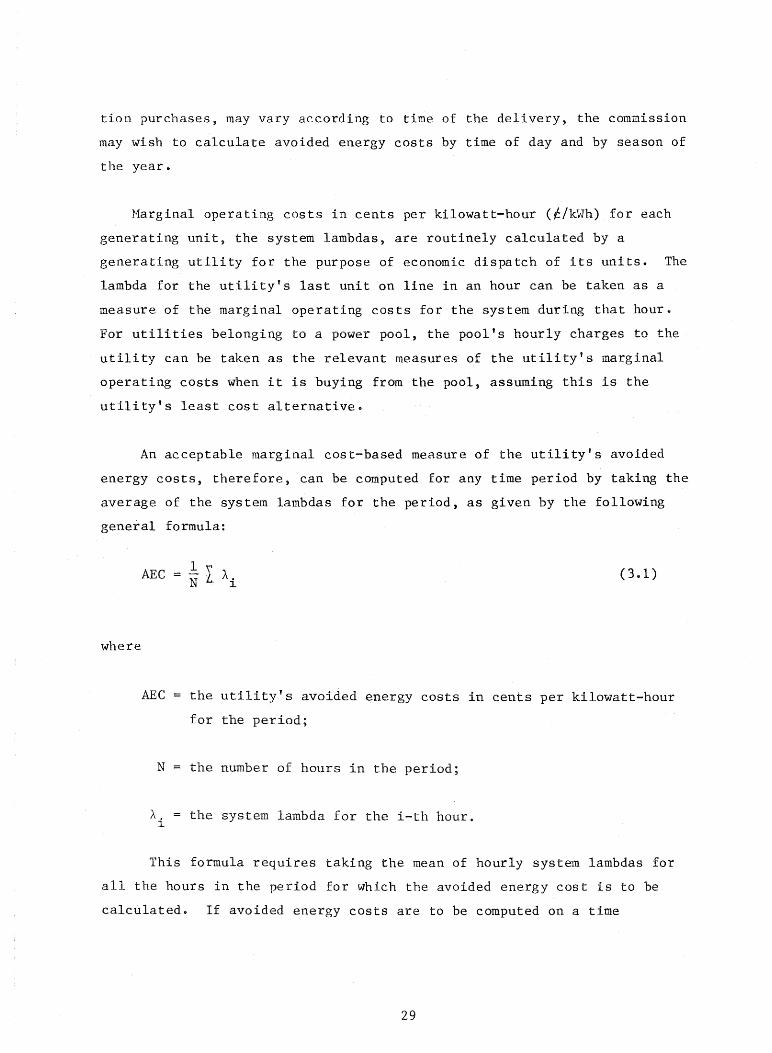
An acceptable marginal cost-based measure of the utility's avoided

energy costs, therefore, can be computed for any time period by taking the

average of the system lambdas for the period, as given by the following

general formula:

where

AEC l"L A. N . I. (3.1)

AEC the utility's avoided energy costs in cents per kilowatt-hour

for the period;

N the number of hours in the period;

A. the system lambda for the i-th hour. I.

This formula requires taking the mean of hourly system lambdas for

all the hours in the period for which the avoided energy cost is to be

calculated. If avoided energy costs are to be computed on a time

29

differentiated basis, then separate computations are made for each of the

peak and off-peak periods. In the calculations for each period, N becomes

the number of hours in the period and the Ai's are the lambdas for each

one of the hours. The formula can also be used for computing a utility's

avoided energy cost for a one-year period, without any time differentiation

for peak and off-peak. In this calculation, N equals 8,760 (the number of

hours in a year) and the A. 's are the utility's system lambdas for each 1

of those hours. The resulting avoided energy cost is an average measure

applying to all hours of the year.

In some circumstances, the commission may want to have the utility

pay an avoided energy cost credit that recognizes the varying quantities of

energy to be delivered by a supplier over the various hours of the per­

iod. 4 Such an avoided energy cost estimate can be computed by weighting

the hourly lambdas according to these varying quantities, as shown by the

following equation:

where

AEC I Wi Ai (3.2) i

Wi the fraction of total energy in the period that is expected

in the i-th hour.

As the total amount of energy being supplied to the utility increases,

these equations 3.1 and 3.2 will tend to overestimate its avoided energy

costs unless system lambdas are adjusted. As the most costly utility

generating plants are displaced by cogeneration purchases, the system's

marginal running costs (lambdas) for self-generated power decline.

4This may be the case, for example, when cogeneration purchases are available only during certain hours of the day.

30

Purchases of Energy and Capacity: An Idealized Method

Firm power deliveries and those which may be individually stochastic

in nature but have firm characteristics in their aggregate (e.g., the

collective output of solar and wind po\vered generators) can result in a

utility's avoiding both the capacity and energy costs of electric

generation. The nine step process presented below comprises ""hat may be

thought of as an idealized method for calculating these costs. The bulk of

the method deals with estimating avoided capacity costs. Perhaps the most

critical step in calculating a utility's avoided cost per kilowatt of

capacity purchased from cogenerators is specifying the total amount of

utility capacity displacement that will result from such purchases. The

nature and magnitude of cogeneration supply determines the numher and type

of planned plant additions that the utility may be able to delay or cancel.

The number and type of plants delayed or cancelled, in turn, determines the

utility's total and unit (dollars per kilowatt) avoided capacity costs.

Step 1. Forecast customer demand for electricity over the duration of the

utility's capacity expansion planning period. 5 Call this the utility's

base case forecast.

Step 2. Run a system capacity expansion planning model using as input this

forecast of demand to determine the least cost means for the utility to

meet this base case forecast.

The output of this run should include a schedule of plant additions

and the present value of the capital and operating costs of generation

required to meet the base case forecast. 6

5The length of capacity expansion planning horizons may vary among utilities. For this idealized method, the horizon should be set at that point in the future beyond which costs incurred (or avoided) by the utility are insignificant when discounted back to the present to account for the time value of money, ignoring the effects of inflation.

6He assume the model calculates these present values. For discus­sion of how to calculate the present value of a future expenditure, consult a standard engineering economics text) e.g., H. G. Theuesan, W. J.

31

Step 3. Determine whether the utility has planned capacity additions

and/or firm power purchases that could be postponed or cancelled as a

result of making cogeneration purchases.

If the result of Step 2 shows that the utility should plan neither to

construct nor purchase additional generating capacity over its capacity

planning period, or that it has as planned additions only that construction

in progress that cannot be prudently delayed, then no capacity costs can be

avoided by the utility as a result of cogeneration purchases, and it would

be inappropriate to permit avoided capacity credits in the cogeneration

rate. 7 The utility can avoid only system operating costs in these

situations; to calculate its avoided cost, refer to the subsection,

"Purchases of Energy," above.

If the utility has planned capacity additions and/or firm power

purchases that could be delayed or cancelled, proceed to Step 4.

Step 4. Forecast the probable amount of firm cogeneration supply that will

develop in the utility's service area during the period for which rates

will be in effect.

Fabrycky, and G. J. Theusan, Engineering Economy, 4th edition (Englewood Cliffs, N. J.: Prentice-Hall, Inc., 1971), pp. 105-8.

7Uowever, in line with the provisions of §292.303 of the PURPA, Section 210 rules, a cogenerator may request the utility to transmit its power to another utility with which the utility is interconnected. The first utility may agree to wheel the power to a second utility or it may decline to do so. If it agrees, then the second utility must purchase the cogenerator's electricity at its (the second utility's) own avoided cost, less an appropriate amount for line losses. The first utility need not agree to wheel the cogenerated power, but if it does not agree, it retains the obligation to buy at its own avoided cost. Cogenerators may wish to pursue this wheeling option for selling their output when the utility in whose service area they are located has excess capacity, is a non-gener­ating utility, or is a small utility with avoided costs lower than the cogenerator might obtain if located elsewhere.

32

A reasonable forecast of the anticipated capacity value of this

cogeneration supply is needed to determine how the utility's capacity

expansion plan will be affected by this new source of capacity supply. A

part of this forecast is a determination of the number of years duration of

this firm power; i.e., will it be available for one year, five years, or

permanently? The length of time over which firm power is supplied affects

how long a plant addition may be delayed and, within the context of the

utility's capacity expansion planning horizon, whether it may be cancelled

altogether. The duration of firm supply, therefore, is one factor that

determines the total long-run cost of capacity that the utility avoids. To

simplify the presentation, we assume here that the forecast of cogener­

ators' supply of firm power extends through the utility's planning horizon.

This supply can be considered permanent for utility capacity planning

purposes. When this is not the case, the ratemaker will find it necessary

to make separate avoided capacity cost calculations and set separate

capacity credits for sources of firm power with different supply durations.

It should also be noted that this forecast of cogeneration supply is

limited to the firm power supply that becomes available during the period

for which the rate for purchase is to be paid. Firm power that first

becomes available after this period is not included in the forecast.

Step 5. Modify the utility's base case load forecast (obtained in Step 1)

by the amount of forecasted firm capacity and energy supply from cogener­

ators (obtained in Step 4). Call this the utility's modified forecast.

The result of Step 5 is a modified utility load forecast (more cor­

rectly, modified forecast of its generating requirements) that takes into

account the forecasted supply to be purchased from cogeneratorso

Step 6. Run a system expansion planning model to obtain a new optimum

system expansion plan for the modified forecast (obtained in Step 5).

33

The output of this run will be a new optimum schedule of utility

capacity additions (other than the capacity purchased from cogenerators)

needed to meet its modified forecast. Also included in the output should

be the present value of the total capital and operating costs of generation

required to meet the modified forecast.

Step 7. To find the present value of the utility's long-run avoided cost

due to the firm supply of cogenerators, subtract the sum of capital and

operating costs obtained in Step 6 from the sum obtained in Step 2.

The result of Step 7 is the difference in present values of the

utility's total generation costs (capacity and energy) associated with

meeting the base case and modified case forecasts, the latter of which

takes into account the firm power supply of cogenerators.

Step 8. Annualize the Step 7 result.

Assuming that the present value of the utility's long-run avoided cost

is not to be paid to the cogeneration suppliers in a one-time, lump sum

pa~nent, this step is needed to find an annual installment on this cost

appropriate for ratemaking. Annualized costs can be obtained according to

the following general formula.

PVAC = PVTC~_(l!~R)-~

where:

PVAC present-value annualized cost;

PVTC present-value total costs;

and the expression in parentheses is an annuity factor in which:

34

IR interest rate;

N number of years over which the cost is annualized.

T,vith firm power supply that is permanent, one can take N to equal infinity

(00).8 In doing so the general formula reduces to the expression:

PVAC PVTC(IR)

Step 9. To obtain a unitized measure of the utility's long-run avoided

cost, divide the Step 8 result by the annual amount of electricity in

kilowatt-hours supplied by cogenerators.

However, the way in which unit avoided costs are calculated ultimately

depends on the way in which these costs are to be paid to cogenerators.

For example, a commission may want to allow either dollar-per-kilowatt or

cents-per-kilowatt-hour payments of avoided capacity costs, depending on

facility size, metering considerations, and whether the credit is for a

class aggregate capacity value or whether it applies to the output of one

facility. The commission may also want to adopt rates for purchases that

vary by time of delivery. For discussion of these types of ratemaking

considerations, see the following section, "Rates Based on Avoided Costs."

If this method of computing avoided costs is used and separate

measures are desired for the utility's dollar-per-kilowatt avoided cost of

81£ the firm supply is not permanent, then a finite value for N may be appropriate. The commission will probably choose to set N equal to the number of years for which the cogeneration capacity is considered firm. This increases the value of the annuity factor, but shorter-term capacity supplies also create less difference in the utility's optimum expansion plan so that PVTC is lo\.ver and, on balance, the PVAC Hill also be lovver, ceteris paribus.

In practice, any firm supply that extends through the utility's planning horizon can be considered permanent. Without specific information that a source of firm supply is temporary, it should be treated in the same way for avoided cost analysis as increments in demand are treated in ordinary marginal cost analysis. That is, ~"hatever annuity factor is used for calculating utility customer annuity payments should also be used for the utility's payment of avoided cost to its cogeneration suppliers.

35

generating capacity and its cents-per-kilowatt avoided cost of energy, then

the capital and operating cost portions of the output from Steps 6 and 2

should not be combined before performing the subtraction called for in Step

7. The annualized differences in capital and operating costs of the two

expansion plans then are divided in Step 9 by the annual kilowatts and

kilowatt-hours, respectively, of firm capacity and energy supplied by the

cogenerators.

This method of calculating avoided cost has been presented as an

idealized one in the sense that it assumes the availability of perfect

information and computational aids (computer models). A discussion of its

practical limitations is in order. First of all, some of the long-term

forecasts that it calls for are in practice impossible to do with any

reasonable degree of certainty. They depend heavily on knowledge of future

economic events that cannot be well predicted given the current state of

the art and science of economic forecasting. Fuel prices are a prime

example. As a result, one may prefer not to calculate a utility's avoided

energy costs for firm power supply by an expansion modeling process such as

the one described above, especially when more direct measures of system

marginal operating costs are available. One may choose instead to

calculate avoided energy costs using equation 3.2 with up-to-date hourly

system lambdas (see the preceding section, "Purchases of Energy").

Secondly, it is true that forecasting cogeneration supply and reoptimizing

the utility's expansion plan properly takes into account the size, timing,

and duration of cogenerators' firm supply when calculating the utility's

avoided cost of generation capacity_ However, such a process also yields a

measure of avoided capacity cost that is unadjusted for the higher unit

energy costs that the utility may incur as a result of delaying or

cancelling new plants. Given the mechanics of the method, there is no

simple way to estimate these costs and to adjust for them. Simpler methods

for estimating a utility's marginal cost of generating capacity, on the

other hand, typically share one common feature: they dispense with

forecasting and reoptimization of system expansion plans. This can be both

a weakness and a strength. When demand increments and decrements are

36

large, the distortions introduced by not reoptimizing the system expansion

process may be substantial. One of the strengths of these simpler

procedures, however, is that adjusting for changes in system fuel

efficiency as a result of adding or not adding a particular type of plant

at a particular time can he estimated and accounted for in a straight­

forward manner.. We examine the application of one of these methods in the

following subsection of this report.

Purchases of Energy and Capacity: A Simplified Method

The idealized method presented above for calculating a marginal cost

based estimate of utility avoided energy and capacity costs may be imprac­

ticable as a solution to the avoided cost estimation problem in many

situationso Here we present a simpler marginal cost approach for calcu­

lating a utility's avoided capacity cost. It is based on the work of

Turvey (see footnote 1); has been applied by Cicchetti, Gillen, and

Smolensky, Ope cit., in developing a computer program called MARGINALCOST;

and is illustrated in Storch, Ope cit. We will refer to the method as the

MARGINALCOST method. The MARGINALCOST approach to long-run avoided cost

estimation simplifies the nine-step idealized method in that it bypasses

the prescribed forecasting (Steps 1 and 4) and capacity expansion modeling

procedures (Steps 2 and 6). To the extent that such a simplified method

can be used in estimating the marginal costs to a utility of expanding its

electricity supply, it can also be used (with some modification) in

estimating the utility's avoided costs associated with reductions in future

generation resulting from the purchase of cogenerators' capacity and

energy.

In order to make the task of estimating marginal costs more

manageable, the MARGINALCOST approach to capacity cost estimation has two

significant simplifying steps: it dispenses wi th forecasting load

increments and with reoptimizing the utility capacity expansion plan for

meeting the incrementalload .. 9 Instead, it assumes that the utility

9This discussion draws heavily upon Storch, Ope cit., ppe 10 ff.

37

response to a load increment is to advance its current expansion plan by

one year. The utility's marginal cost of generating capacity is then

calculated by taking one year of the annnualized capital costs of each

plant whose on-line schedule is advanced,' adding the fixed operation and

maintenance expenses for each plant, and subtracting the total fuel savings

to be realized by having brought a newer, more efficient plant on line one

year earlier. These costs are converted to current dollars, summed,

increased by factors that account for required reserve margin and line

losses, and then divided by the sum of the rated capacities of the affected

plants= The result, expressed in $/kW) is taken as an estimate of the

utility's long-run marginal cost of expanding generating capacity.

In the avoided cost calculation problem, one is required to estimate

long-run decremental costs. Where utilities are planning future capacity

additions and the MARGINALCOST method can be applied to estimating

incremental capacity costs, it can also be applied (in the reverse) for

estimating capacity savings. Instead of moving the utility's expansion

plan forward, one moves it backward. The cost calculation and variables

entered into it are then the same for decremental (avoided) costs as for

incremental costs, with two exceptions:

1) instead of fuel savings being realized, additional fuel

expenditures are incurred as a result of having less

efficient plants on line one year longer; these additional

fuel costs are subtracted from the year of annualized

capital and fixed O&M expenses avoided for each plant as a

result of moving the expansion plan back; and

2) no adjustment for reserve margin requirements or line losses

needs to be made because the utility generally does not

avoid these costs as a result of making power purchases.

Taking these differences into account, a marginal cost based estimate of a

utility's avoided capacity costs can be calculated by a procedure similar

to that presented in Table 3-1.

38

The utility expansion plan and cost data in Table 3-1 are hypothet­

ical, constructed to approximate current costs. The hypothetical planned

additions are two 800 ~~ (800,000 kW) base load units, one coal and one

nuclear, scheduled to come on line in 1982 and 1985, respectively. All

costs are expressed in 1981 dollars, the year in which the avoided-cost

cogeneration rate will be paid. Line (1) contains the total capital cost

of each facility, and line (3) presents one year of these costs annualized

at a 10% interest rate over a 30-year life for each plant. Line (4) is the

annual fixed O&M expenses for each unit. Instead of fuel savings from

advancing new plants, line (5) in the avoided-cost calculation table

becomes the additional fuel and variable O&M expenses from having older,

TABLE 3-1

HYPOTHETICAL UTILITY AVOIDED COSTS OF GENERATION CAPACITY (IN KW) USING THE MARGINALCOST APPROACH (1981 DOLLARS)

Coal Plant Nuclear Plant Item (On Line in 1982) (On Line in 1985)

(1) Capital Cost $ 480,000,000 $ 800,000,000

(2) Capacity (kW) 800,000 800,000

(3) Annual Capital Costa $ 50,928,000 $ 84,880,000

(4) Annual Fixed Operation

and Maintenance Cost 1,320,000 1,200,000

(5) Additional Fuel Costs 12,000,000 24,000,000

(6) Total Avoided Costs of

Generation Capacity

(3) + (4) - (5) 40,248,000 62,080,000

aBased on a 30-year life and a 10% interest rate.

Source: Hypothetical data and calculations.

less efficient plants on line one year longer. 10 Line (6) presents an

esti.mate of the present value of the utility's net avoided generating

10Since both of the plants in this example are 800 MW base load

39

capacity cost for each plant as a result of delaying their introductions by

one year. This quantity is calculated by adding the annualized capital

cost of the plant to its annual fixed O&M expenses and subtracting the

additional fuel expense associated with the operation of older plant(s) one

year longer.

The utility's avoided capacity cost per kilowatt is then calculated by

summing the net avoided capacity costs for each unit and dividing by the

summed kilowatt capacities of the units. For this example:

$40,248,000 + $62,080,000 = $63.96/kW11 800,000 kW + 800,000 kW

To convert this estimate to cents per kilowatt-hour, one divides by 8,760,

the number of hours in a year.

The MARGlNALCOST computer program does not calculate incremental or

decremental energy costs; it requires them as an input. 12 One approach to

calculating these costs has already been described, the averaging of hourly

system lambdas. For instructions, see preceding section, "Purchases of

Energy ...

For those without computer capabilities or who would otherwise choose

to calculate avoided costs by hand, the MARGINALCOST calculations are

relatively simple and, given the necessary input data, can be performed

with the aid of a calculator in a few hours. 13

plants, growth in the utility's generating load is ignored in calculating additional fuel expense. It is assumed that these plants will be in constant operation no matter what year they are introduced.

llIn the MARGINALCOST procedure this number is multiplied further to account for required reserve margin and line losses for transmission (by voltage level). Since these costs are not avoided by the utility as a result of cogeneration purchases, these multipliers are inapplicable to avoided cost calculation.

12Storch, Ope cit.

13See Cicchetti, Gillen, and Smolensky, Ope cit.

40

Rates Based on Avoided Costs

How Avoided Costs Are to Be Paid

Once a utility's avoided costs have been calculated, the commission

must decide how these costs will be paid to cogenerators. If time-of-day

metering is already installed on the premises or if its installation is

judged to be cost-effective based on the anticipated volume of cogenerator

sales to the utility, the commission may want to adopt rates for purchases

that vary by time of day. If this option is chosen and the commission has

not already done so, utility rating periods for pricing these transactions

will have to be defined. 14 To do so, the commission must decide what

method it will use for determining the relative amount of avoided capacity

costs that will be paid for deliveries during peak and off-peak periods. 15

Avoided energy costs must also be calculated for peak and off-peak periods

(see "Purchases of Energy," equation 3,,2).

In setting rates for cogeneration purchases, the commission must also

determine whether and under what conditions avoided capacity credits will

be paid on a dollar-per-kilowatt or a cents-per-kilowatt-hour basis. If

capacity credits are to be awarded for only firm deliveries under contract,

then avoided capacity costs can be paid on a dollar-per-kilowatt basis for

the minimum deliverable capacity in the contract, much in the same way that

large consumers of electricity are billed a dollar-per-kilowatt charge for

the maximum demand they are permitted to place on the system. Aggregate-

14For an example illustrating how to go about selecting peak and off-peak periods, see Electric Power Research Institute, Electric Utility Rate Design Study, "How to Quantify Marginal Costs: Topic 4," Chapter IV, pp. 25-33.

lSrhere are at least three methods for distributing capacity costs to utility rating periods. For a treatment of the MARGINALCOST method, see Storch, Ope cit.; for the NERA method, see Electric Power Research Institute, Ope cit., Chapter V; and for the EBASCO method, see Electric Power Research Institute, Electric Utility Rate Design Study, "Costing for Peak Load Pricing: Topic 4," ppe 83-88.

41

value avoided capacity cost credits (paid to a class of producers whose

deliveries are individually random in nature) will generally have to be

determined on a cents-per-kilowatt-hour basis.

Interconnection Costs

The FERC rules, §292.306, require each qualifying cogeneration and

small power production facility to pay the necessary costs of inter­

connection with the electric utility power grid. State commissions are

left to determine the proper amount of these costs, as well as the manner

and term for their reimbursement to the utility. The assessment of these

costs must not discriminate against the qualifying facility in comparison

with the utility's practices toward other members of the same customer

class who do not generate electricity; i.e., cogenerator and small power

producer interconnection charges are limited to the amount of additional

interconnection expense that the utility incurs in order to permit

purchases to be made. The FERC rules also permit these charges to be

included in calculation of standard rates for purchases.

A recent survey sponsored by the U.S. DOE16 has uncovered wide

variation in utility interconnection practices and attendant costs. It

also has found that the criteria for evaluating such practices is far from

standardized. This lack of uniformity reflects in part individual

utilities' varying philosophies regarding acceptable risk and reliability

performance, as well as the fact that protective relaying has long been

regarded as an engineering art, affected by designers' judgments about the

trade-offs between reliability and cost. Actual interconnection costs were

found to range from $60,000 to $691,000 for customers whose capacities

ranged from 20 kW to 20 MW. Interconnection requirements appear to be

heavily situation-dependent and not necessarily related to the size of the

facility_ The report recommends that interconnection costs be determined

16James B. Patton, Survey of Utility-Cogenerator Interconnection Practices and Costs, Final Report to the U.S. Department of Energy, Office of Electric Energy Systems (Palo Alto, California: Systems Control, Inc., June 20, 1980.)

42

on a case-by-case, component-by-component basis, and cautions against

making generalizations from "typical" cases described in its survey. A

review of the engineering aspects of interconnection, especially as they

relate to concerns about system safety and reliability, is contained in a

recent paper by Blair Ross, American Electric Power Service Corporation. 17

l7Blair A. Ross, "Cogeneration and Small Power Production Facility Effects on the Electric Power System," Paper presented at The National Regulatory Research Institute Conferences on FERC Cogeneration and Small Power Production Rules and their Impact on State Utility Regulation, June 17-27, 1980.

43

~ ;.:d G H

~ 0 0

~

~ tlj

~ ~ 'i:I Z ;J> G ~ I'%j 0 H ;.:d H

H

~ tlj :;;d

§ ~ H t:i:I t:;l CIl tlj

~ <l H 0 tt:l

CHAPl'ER 4

INTRODUCTION TO INTERRUPI'IBLr~ SERVICE RATEMAKING

Although much of the recent increase in electricity prices has been

due to factors beyond utilities' direct control (e.g., fuel expenses,

construction costs, and costs of implementing environmental regulations),

reduction in the growth of expensive peak demand is one area that still has

significant cost control potential for many utilities. If system load can

be reduced during extreme peak periods, considerable savings in present and

future fuel and equipment expenditures often can be realized.

The term "load management" refers to a variety of methods that a

utility may employ to alter the pattern of demand reflected in its load

curve. Load management techniques may be either direct or indirect in

nature. Indirect techniques rely on incentives to induce consumers to

regulate voluntarily the demands they place on the system. Time-of-use

rates can be thought of as an indirect load management technique. Direct

load management techniques allow the utility to control by electro­

mechanical means some portion of the system load. Interruptible rates are

an example of a direct load management technique. Customers who choose

interruptible service agree to allow the utility to cut off their

consumption of electricity when th(~ utility is unable to meet total system

demand due to insufficient capacity.

While interruptible tariffs are common to many utilities, the practice

of interrupting interruptible customers may vary widely from one company to

another. It appears that some utilities may have created interruptible

rates (for certain industrial customers, for example) but proceeded to plan

and construct capacity as though the subscribers were regular, assured

47

seLvice customers. l This practice, where it has existed, violates one of

the cost-based rationales for creating an interruptible class in the first

place: to conserve capacity and energy costs on peak.

Nonetheless, interruptible service is still one tool available to

utilities with the potential for improving system load factor and, hence,

reducing required peak Generating capacity and peak fuel consumption. In

addition, it can be seen as a vehicle for providing greater choice by

consumers in selecting the kind of electricity they buy.

Electricity and Product Differentiation

The term "product differentiation" refers to the process of creating

in the minds of conSUI1:=rs real and imaginary product differences associated

with an industry's output. For example, the auto industry produces and

sells a product that is highly differentiated. Consumers view Fords as

being quite distinct from Chevrolets. Indeed, the many options available

on a typical automobile mean that even two cars of the same make and model

will typically have distinctive features such as color, interior design,

and varying mechanical options (air conditioning, automatic transmission,

etc.). Product differentiation can also be based on the purely subjective

preferences of consumers. A good example r.vOllld he the long standing

preference for cane sugar over beet sugar, even though the two products are

chemically identical. Producers may also use advertising to make their

product seem preferable over another. However, much product differentia­

tion is associated with real and important differences in the nature of

product offerings, and it has the effect of creating greater choice for the

consumers in what kind of prO(l11et they buy and how much they will pay for

it.

IThe actual behavior of utilities in this area is difficult to document. The belief that at least some utilities have operated in such a manner is as C.011111l)ll 111 the regula tory communi ty as are denials by utility representatives that their own companies have ever engaged in such a practice. Systematic evidence on the subject seems to be lacking.

48

For a long time in the United States electricity has been different­

iated on the basis of the voltage level at which service is provided.

Utilities have traditionally offered several distinct types of electric

service (i.e., industrial, primary, and residential), based roughly on the

voltage level at which the customer can be served.

Recently, the adoption of time-of-use pricing of electricity in some

service areas has allowed further differentiation of a utility's product.

To a large extent the usefulness and hence value of electricity to

consumers depends upon the time at which it is consumed. A kilowatt-hour

of electricity provided from 3 a.m. to 4 a.m., for example, is usually not

a ~()O,.l sl\1Jsti tute for a kilowat t-hour provided from 3 p .. m. to 4 p .. m.

Similarly, the cost of producing each of these kilowatt-hours differs

g-rea tly from that of the other. Seasonal and time-of-day rates recognize

electricity as a product that is differentiated on the basis of the time it

is produced and consumed.

The concept of interruptible electric service is another means for

utilities to further differentiate their output. This differentiation is

based on the reliability level at which electricity is received. With an

interruptible service option, customers are offered the opportunity to

choose a service reliability appropriate to their needs, presumably at a

rate lower than that charged for regular (firm) service.

Value-Based versus Cost-Based

Pricing of Interruptible Service

In the past, interruptible service options have been offered by

utilities at rates lower than those charged for regular service. Most of

these have taken the form of individually negotiated contracts between the

utility and one or more of its large industrial users. These special

contract services were often created to induce potential high-volume,

high-load-factor customers to use utility-generated electricity as their

primary energy source, rather than self-generating their electricity or

using some competing energy form such as fuel oil or natural gas. As

49

implied by the existence of individualized service contracts, the price of

this interruptible electricity was negotiated and was usually based on the

value of the service to the customer. For the industrial customer with

potential for self-generation, for example, the finally negotiated price

would lie somewhere between the utility's own running costs and those the

customer could expect to incur if he were to produce tl~ el~ctrlcity

himself. With the utility's more efficient, large central generating

stations, presumably the latter would be greater than the former&

Therefore, the interruptible contract based on value-of-service is an

arrangement under which both the utility and the industrial customer can

benefit.

Provisions of the PURPA and the general concern of ratemaking

authorities about setting e'1uti.:.qhll~ utility rates, however, have brought

cost-of-service principles to the forefront in discussions of electric

ratemaking. The PURPA Section III ratemaking standard for interruptible

service, for example, states:

Section III (d) (5) INTERRUPfIBLE RATES - Each electric ntility shall offer each industrial and commercial customer all i.rli.:p.rruptible rate which reflects the cost of providing interruptible service to the class {)f wh1.ch such customer is a member.

What we present in this report is an exploration of one approach to

pricing interruptible service on the basis of the costs of providing that

service, the marginal cost approach. Not all agree that marginal cost is

the appropriate standard to use when calculating cost-of-service, but

marginal costing clearly lies on the cost-of-service rather than value-of­

service side of approaching this particular ratemaking problem.

Load Management, Capacity Planning, and the

Reliability of Interruptible Service

Effective utilization of interruptible service by utilities in their

overall load management program can provide excellent opportunities for the

50

realization of two of PURPA's ratemaking goals--efficiency in utility

operations and conservation of scarce energy resources. If interruptible

cates are properly set at the cost of providing interruptible power, the

third of PURPA's goals--equity toward ratepayers--will also be served.

More specifically, providing an interruptible rate and strategically

shedding the load of customers who select it can result in the postponement

of expensive capacity additions and the conservation of scarce and expen­

sive peaker fuel. Offering an appropriately reduced rate to customers who

select the option can also provide an incentive for customer shifting of

unnecessary peak loads to off-peak hours, thus improving system load factor

and promoting utility efficiency.

While having an interruptible rate ideally can result in the above

favorable developments in utility operation, past experience with

interruptible rates suggests that, in some cases, the ideal has not been

realized. Despite being classified as "interruptible," many customers have

seldom had their electricity cut off. At the same time, the utility has

continued to build new generating capacity. One is tempted to conclude in

these sitlffitions that some of this capacity may have been planned to meet

interruptible loads. This practice, where it exists, furthers neither

at Lli Lj efficiency, conservation, nor equi ty ..

One solution to this problem is for the state utility commission not

to approve for inclusion in the utility's construction plans those capacity

additions associated with meetir~ interruptible customer's load; Not per-

mitting such raising of capital would in a way solve the problems of equity

and efficiency. Planning no capacity for interruptible service, however,

creates another problem: the threat of very low or highly unstable

reliability levels for interruptible service customers.

When a utility plans no capacity additions to serve the needs of

interruptible customers, the frequency of interruption for interruptible

customers can become high and/or irregular, depending on the number and

load patterns of customers selecting the option, and the coincidence of

their demands with the regular, assured-service customers. For some inter-

51

ruptible customers (e.g., those who can reschedule most consumption to

off-peak hours), these frequent or unpredictable patterns of interruption

on peak may be of no concern. Their main interest, due to high volume

consumption, is in receiving a lower rate. Other potential interruptible

customers may he interested in a somewhat reduced rate and could

accommodate occasional interruptions of service, but only relatively

infrequently and only when the frequency, timing, and duration of

interruptions could be predicted with some reasonable degree of certainty.

One approach to resolving this problem is to create two classes of

interruptible service, one for which some utility generating capacity is

planned (Class I) and a second for which there is not (Class II). Each

faces a different rate. For Class I, a lower than no~al reliability level

would be specified and generating capacity built to meet this level.

Providing power to Class I interruptible service at a reliability level

lower than regular service would result in a lower cost of service and

preserves the potential for a reduced rate. Specifying a minimum for Class

I reliability, however, also resolves the problem of too frequent or

unstable patterns of service interruption. Class II interruptible, on the

other hand, would have no minimum reliability and would be served only by

the utility's available idle capacity. This preserves the opportunity for

power consumption at the lowest possible cost.

Creating such interruptible service options to go along with regular

(firm) service, however, can create some formidable costing problems for

the cost-of-service analyst, not to mention the initial problems posed for

t:h~ utility's marketing department in selecting the proper reliability

levels at which service should be offered.

The Economics of System Reliability and Interruptible Electric Service

The reliability of electricity supply systems and selection of optimum

plant capacity have been subjects of increasing professional interest among

utility engineers and economists in recent years. Much of their work has

dealt with the problem of determining the optimum plant capacity that a

52

utility should construct to generate electricity_ The optimum capacity of

an electric utility refers to the plant and equipment that allows the

utility to serve its customer load at the lowest possible cost, taking into

account the costs associated with power outages. Optimum capacity depends

not only on the magnitude and pattern of customer load but also on the

desired reliability level of electric service.

Many utilities use a "loss of load probability" (LOLP) of one-day-in­

ten-years as a target for system-wide reliability. Use of this standard

rnearlS tlv-lt the total amount of time that a utility would be unable to meet

customer demand would be one (24-hour) day in a ten-year period. This

level of reliability requires that the utility build and maintain some

generation capacity that is used relatively infrequently. Utilities in

other countries, such as France and Great Britain, typically maintain

electric service reliability levels considerably lower than those in the

United States. The U.S. typically experiences a loss of 1.75 hours of

electrical service per customer per year. France and Great Britain

experience a 6 hour and 17.5 hour annual loss per customer, respectively.2

This high level of reliability of electrical service in the United States

might be admirable were it not for the fact that maintaining it is quite

expensive. 3

Michael Telson has attempted to estimate the social costs (e.g., lost

industry output, spoilage, etc.) associated with electric outages. He

found the social costs to be well below the costs of the additional plant

2Michael Telson, "The Economics of Alternative Levels of Reliability for Electric Power Generation Systems, II Bell Journal of Economics, (Autumn 1975), ppe, 679-94.

3U.S. Congress, House Subcommittee on Energy and Power, Committee on Interstate and Foreign Commerce, Are the Electric Utilities Gold Plated? A Perspective on Electric Utility Reliability, Congressional Research Service, Library of Congress, 96th Congress, 1st Sesse, April 1979 (Washington, D.C.: UeS. Government Printing Office, 1979). For a look ahead at the expected future of utility service reliability given

53

capacity needed to avoid the outages. 4 Using a quite different technique

for estimating the social costs of an outage, Munasinghe and Gellerson

found that the power system of Cascarel, Brazil could realize substantial

savings by choosing a lower level of reliability than is traditional, and

yet stIll maintain a satisfactory level of service reliability.5 In this

stll(ly) the cost of power failures to society includes the costs of

interruption of production in other industries, spoilage, and the

disruption of leisure time activities by households. Indeed, the loss of

leisure time activities is considered the chief outage cost for residential

consumers according to Hunasinghe and Gellerson. 6

In sum, the work of Telson and Munasinghe and Gellerson suggests that,

from an economic perspective, th8 tl~ditional reliability levels of

electric utilities may be excessive (i.e., the cost of very high

reliability may exceed the costs that would be imposed on society by an

outage). The ideal reliability level and hence the optimwn capacity of the

utility, they suggest, requires comparison of the social cost of outages

with the cost of maintaining given levels of reliability in electricity

supply.

The well known Averch-Johnson thesis holds that regulated public

utilities have an economic incentive to increase their rate base through

excessive investment in plant and equipment. 7 Additional theoretical

alternative demand and supply scenarios, see: U.S. Congress, House Subcommittee on Energy and PovJer, Committee on Interstate and Foreign Commerce, Will the Lights Go on in 1990? Congressional Research Service, Library of Congress, 96th Congress, 2nd Session, August 1980 (Washington, D.C.: U.S. Government Printing Office, 1980).-

4Telson, Ope cit., pp. 685-690.

5Mohan Munasinghe and Hark Gellerson, "Economic Cri teria for Optimizing Power System Reliability Levels," Bell Journal of Economics, (Spring 1979), pp. 362-3.

6Ibid", p. 356.

7H. Averch and L. Johnson, "Behavior of the Firm under Regulatory Cons traint , .. American Economic Review, (December 1962), pp. 1053-69.

54

support for the view that a rate-of-return regulated monopoly may tend to

choose levels of reliability in electric service which exceed the socially

optimal level has been provided by Crew and Kleindorfer&8 Empirical

evidence bearing on the general form of the Averch-Johnson hypothesis is

mixed,9 but the results of reliability studies performed to date suggest

that the costs of maintaining reliability levels traditional to U.S.

utilities may exceed the economic benefits derived by consumers&10

Creating an option of interruptible electric service has the advantage

of allowing consumers to participate directly in the choice of the system's

total reliability level. As more customers opt for interruptible service,

less total capacity is required by the utility. With lowered reliability,

of course, may come reduced capital expenditures. Properly priced, inter­

ruptible and regular service options give correct price signals to

consumers regarding the capacity cost implications of their reliabilty

demands, and allow customers to decide the utility service reliability

level that they both want and are willing to pay for. Customers who want

highly reliable electric service are permitted the option of purchasing

non-interruptible electric service exclusively, but they also will be

required to pay a price reflecting the costs associated with providing it.

Cost based pricing of interruptible electric service has received

attention only recently. Marchard11 has developed a model of socially

optimal (marginal cost) pricing of electric service supplied at alternative

levels of reliability_ Unfortunately the model does not take into account

the correlation of the electricity demands of individual subscribers (e.g.,

hot weather may increase the electric demands of many consumers simultane-

8M. A .. Crew and P. R .. Kleindorfer, "Reliability and Public Utility Pricing," American Economic Review, (March 1978), pp .. 38-9 ..

9Daniel Z. Czamanski, et al., Regulation as a System of Incentives (Columbus, Ohio: The National Regulatory Research Institute, 1980) ..

10Telson, Ope cit.; and Are the Electric Utilities Gold Plated?, Ope cit ..

11M .. G .. Marchard, "Pricing Power Supplied· on an Interruptible Basis,"European Economic Review, (July 1974), pp. 262-274 ..

55

ously),,12 This deficiency suggests that a complete theoretical solution

to the problem of interruptible electric pricing has yet to be offered.

A recent article by Panzar and Sibley develops a model that

incorporates another approach to the problem of pricing electric

reliability.13 Under the Panzar-Sibley model, consumers of electricity

nJ'(-~ per1nitted the option of buying a fuse that sets a ceiling level on

their electric demand. Each consumer thereby chooses his 0·;..]l1 level of

reliability in the process of fuse selection. Fuses are priced according

to the utility's marginal cost of capacity. One difficulty with this

self-rationing approach is that it does not account for the diverse timing

of customer loads. An individual subscrC)(~r ';lay exceed his allotted fuse

capacity and be cut off from further consumption during an off-peak time.

Such rationing of consumption is manifestly inappropriate when idle

generation capacity exists.

In conclusion, a review of the current economic literature indicates

that considerable work remains to develop an acceptable, operational method

for pricing interruptible service in a marginal cost framework. An attempt

to develop such a method appears in chapter 5.

Recent State Public Utility Commission Rulings

Information on states' consideration of the PURPA interruptible

service standard from sixteen state public ut iIi ty commissions was

available at the time of this wri ting. The.s(~ 8 ta tes are Arkansas,

Californi.a, Colorado, Connecticut, Florida, Illinois, Kansas,

Hassachusetts, Michigan, New York, North Carolina, North Dakota, Ohio,

South 8arolina, Vermont, and Virginia ..

12I bid., p .. 273.

13John C. Panzar and David S .. Sibley, "Public Utility Pricing under Risk: The Case of Self Ra tioning," American Economic Review, (December 1978), pp. 889-95.

56

Of these sixteen states, seven have some ronn of interruptible service

option in place for i0:1-13 tJAial and commercial customers.. In addition, at

least five of the sixteen states have approved some form of interruptible

residential load-control option.. Eight state public utility commissions

have ordered studies of the industrial interruptible service option and its

feasibility, while six state commissions have initiated studies of

residential load control.

The industrial interruptible service offered by the major Michigan

utilities provides an interesting example of interruptible rate design.

The minimum reliability level for this service is described in terms of a

maximum number of hours of interruption permitted per year (e .. g., 600 hrs ..

or 1,000 hrs .. ) and a maximum of 14 hours of interruption per day. The

ratio of the maximum possible hours of interruption per year to the number

of peak hours per year, mUltiplied by the regular service demand charge

yields the demand charge discount permitted to interruptible industrial

customers. An attractive feature of this method is its operational

simplicity.

Two of the perhaps better known residential interruptible power

service options offered by regulated utilities are in Arkansas and Vermont.

The special interruptible air conditioner rate approved by the Arkansas

Public Service Commission allows Arkansas Power and Light to offer

residential customers with central air conditioning an interruptible

service option. 14 Radio signals are used by the utility to interrupt

consumption. Participating consumers are granted a monthly credit per kva

of air conditioner compressor capacity. In Vermont, the Green Mountain

Power Corporation offers residential customers a five-dollar-per-month

c recii. t for agreeing to wa ter heater load control using a ripple control

system ..

14Raymond We Lawton, et al., Energy Management and Conservation in Arkansas, NRRI-78-1 (Columbus: The National Regulatory Research Institute, i978).

57

For a review of some of the more interesting utility exper.ilnental

programs currently underway involving interruption of customer load, see

the recent article in Public Utilities Fortnightly by Reinbergs and

Harlan. 15

The Perspective of Industrial Consumers

In general, industrial consumers are on the record as favoring

introduction of interruptible rates. 16 At the same time, there seems to

be little support for marginal cost pricing of electricity within this

influential consumer group.17 Hence, an interruptible rate based on

marginal cost pricing principles may encounter some opposition from

industrial consumers. However, the lower net cost of power available to

many industrial customers through llltn),luc.tlon of cost-based reliability

option(s) may reduce much of the tr c::rLticism. Potential cost savings may

be especially magnified in utili ty ,:>(~}." tC(~ areas where the interruptible

option(s) are offered as alternatives to mandatory time-of-day rates for

large users.

l5r1o Reinbergs and Kenneth M. Harlan, "Problems with Direct Load Control by Electr.iJ~ iJtLlities," Public Utilities Fortnightly, January 3, 1980, p. 21. -

16Jay B. Kennedy, "Load Management: Go od Ideas or Not?" ELeON Report (Winter 1979), p. 2.

l7Ibid., p. 5.

58

CHAPTER 5

METHODS FOR COMPUTING THE MARGINAL COST

OF INTERRUPTIBLE SERVICE AND

CONVERTING THESE COSTS INTO RATES

As already suggested in our introduction to interruptible ratemaking,

the problem of defining interruptible service and tracking its system costs

may be made a little easier if one considers it from a variable service

reliability perspective. Since regular electric service in the United

States presumes a comparatively high service reliability, interruptible

service can be defined through the process of selecting appropriately lower

level(s) of reliability that meet candidate customer requirements. The

costing problem for interruptible service then largely centers around

determining the utility capacity expenditures necessary to meet these

reliability requirements. There are also, of course, energy cost

differences related to peak and off-peak consumption and customer-related

metering and load-control device costs that have to be considered in

setting a cost-based interruptible rate. However, determining the costs of

generation, transmission, and distribution facilities necessary to provide

service at prescribed reliability levels is the most challenging costing

problem in calculation of the marginal costs of interruptible service.

As a preface to presenting a method for calculating the marginal costs

relevant to setting interruptible rates, it may be helpful to consider

first the problems of capacity planning and electric service reliability as

they relate to providing this type of service and determining its costs.

59

Capacity Planning, Service Reliability, and Interruptible Service

Perhaps due to the value-of-service pricing tradition in interruptible

service contracts, the cost impact on the utility of providing this service

at varying levels of reliability has received little attention. Large­

volume interruptible customers usually have a reduced demand charge as part

of the interruptible rate, compared to that of regular, firm service, but

detailed cost justifications for these reductions are seldom offered.

Since utility capacity normally used to serve the interruptible

customers' load may be also used on occasion to serve regular service load

(during periods of interruption), the capacity planning and costing

processes are complicated beyond the standard case in which the service

reliability of all customers is homogeneous. In order to prevent the

frequency of service interruptions from becoming intolerably high,

utilities may need to set aside some capacity to serve interruptible load.

It is also clear, however, that some utility capacity cost savings may

result from having interruptible load as an additional reserve for meeting

regular service demand during extreme system peaks. Utilities may use

different decision rules for determining when to meet and when to shed

these incremental demands,l but the impact of interruptible service class

demand on the system's need to incur marginal capacity costs depends

basically on two factors:

lDecision rules are needed for both interruptible class and individ­ual customer load shedding, but we are referring to the former. For example, a utility may decide that it will begin to shed interruptible load as soon as operation of the system's peakers are required. This may be a good rule when a utility is concerned primarily with saving on consumption of peaker fuel. Another utility may decide that it will shed interruptible load when it has to buy power to meet load. Still another utility may interrupt as an alternative to building new capacity. Any of these rules may be appropriate, depending on utility circumstances. In this report, we assume that the utility sheds interruptible load when total system load, including interruptible, exceeds total available capacity_ We assume further that the company stops interrupting and buys or builds additional capacity to meet interruptible demand only when further interruption would violate the maximum amount of interruption provided for in the customer's tariff or service contract.

60

1) the coincidence of this demand with regular, assured service peak

demand; and

2) the service reliability specified in the interruptible tariff or

service contract.

One could reasonably expect that the reliability needs of customers

who may be candidates for interruptible service could actually be quite

different from each other; i.e., their tolerances for interruptions

according to timing and duration may vary markedly. As we have already

suggested, this situation may require the creation of more than one class

of interruptible service, each with a different service reliability level

and, presumably, cost of service.

Another problem that arises in calculating the costs of utility

capacity required to provide interruptible service is that these costs are

composed of two parts: generation, and transmission and distribution (T&D).

Maintaining customer service reliability requires not only sufficient

generating capacity to meet customer load, but also sufficient capacity in

high voltage transmission lines, distribution substations, and line

transformers to handle the load. 2 In practice, most customers are rarely

if ever interrupted for lack of transmission and distribution capacity,

since the utility's network provides multiple routes for reaching most

customers; but most utility outages that do occur in the United States are

due to T&D failures. 3 Industrial interruptible customers, moreover, are

normally large-volume consumers, and they may not be uniformly distributed

geographically over the utility's T&D network. Several industrial

interruptible customers located along the same transmission line, for

example, may be interrupted more frequently due to T&D failure than an

industrial interruptible customer located in a primarily residential area.

2The probability of an interruption is equal to the probability of an interruption due to generation capacity failure, plus the probability of transmission capacity failure, minus the probability of the simultaneous independent failures of both generation and transmission capacity_

3UGS. Congress, Are the Electric Utilities Goldplated?, op.cit., Table 1; for complete citation, see Chapter 4, footnote 3.

61

In this sense, interruptible service customers may compete for the use of

the excess transmission and distribution capacity serving their particular

geographic area if insufficient capacity is planned and built for their

use. The process of planning and determining the cost of this T&D capacity

is complicated by the introduction of reliability levels other than that

normally assumed for regular service. How much sharing will go on between

interruptible and regular service? How frequently will interruptible

service have to be interrupted due to T&D failure for given amounts of T&D

capacity investment and customer load?

A first step toward solution of these costing problems is to make

explicit the reliabilities at which services are to be offered. For the

sake of simplicity, we examine here the case in which two classes of

industrial interruptible services are offered--Class I and Class II. Class

I interruptible customers would be charged for enough generation and T&D

capacity to maintain their reliability at some target level. Class II

interruptible service would have no capacity planned for it or charged to

it, and its reliability would be left unspecified. Such a reliability

ordering of customers would result in Class II interruptible load being

shed first as total system demand exceeds total system capacity, Class I

interruptibles second, and regular service customers last. In some

systems, Class II interruptibles could expect a virtual certainty of

interruption during certain peak demand hours. The actual number of hours

of interruption would depend on the system coincidence and volume of demand

by the individual Class II customer, the coincidence and volume of demand

by other Class II subscribers, as well as the demand of regular and Class I

interruptible customers. The minimum reliability of Class I customers

would be sufficiently lower than that of regular service customers so that

substantial capacity savings could be realized by the utility. The

reliability would be sufficiently high, however, that the frequency of

interruption for Class I would be relatively rare, unlike Class II

subscribers, and the conditions leading up to such interruptions could be

easily identified.

62

In this way, Class I interruptible service would meet the needs of

customers who are sensitive to the price of electricity, but who are also

unable to accommodate frequent or unpredictable patterns of interruption.

For these interruptible customers in the industrial class, electricity

expenses may be such a significantly large portion of total production

costs that a reduction in rate would be worth an occasional rearrangement

of production schedules. However, the costs of labor or fixed overhead,

variable seasonal demand, or the nature of their production processes may

preclude frequent or unpredictable power interruption. From the utility's

perspective, the demand of Class I customers will be served most of the

time by under-utilized capacity, which is only occasionally needed for

regular service demand. In addition, some additional generating capacity

may have to be built to keep these customers' annual loss-of-load

probability (LOLP) below a certain maximum as the volume of their class

demand rises (which is another way of saying that their service reliability

will be maintained at a target minimum). The lower capacity charge and

assurance of long-run stability of reliability levels may act to attract

some large users of electricty to this rate.

Certain other firms, which would make up Class II, may be extremely

sensitive to electricity's price and relatively insensitive to its

reliability, especially during the utility's peak periods. Both the

minimum reliability level and associated capacity charge assessed Class I

customers may be unnecessary for this class of consumers. If lumped with

those selecting a Class I type service, they could be charged for more

reliability than they actually need. For this reason, a Class II

interruptible rate is proposed that includes no capacity charge and that

sets no lower limit on service reliability. Class II customers would be

served by only the utility's capacity left over after it has met regular

and Class I demand. The reliability of Class II service would also be

allowed to vary significantly over time depending on the relative demands

of regular service, Class I, and other Class II interruptible customers.

In summary, Class I interruptible service would offer large users of

electricity the option of receiving service at a lower, but assured,

63

minimum level of reliability with a corresponding reduction in the usual

capacity charge. Class II interruptible service would offer customers a

tariff with no capacity charge in return for service with virtual certainty

of some interruption during peak periods.

Calculating Marginal Cost Based Rates

for Class I and Class II Interruptible Service

This section presents methods for calculating the marginal costs of

generation capacity for interruptible service and a discussion of the

marginal transmission and distribution, energy, and customer components of

interruptible rates. The subsection on generation capacity presents two

methods for calculating a marginal-cost-based generation capacity charge

for the Class I interruptible customer class. The first is an idealized

method, similar in structure and purpose to the idealized method presented

in chapter 3 for calculating utility avoided costs of cogeneration supply.

Like the metlmd in chapter 3, it ignores limitations of data availability,

costs of data acquisition, and availability of resources required to make

computations. The second is a simplified method, also similar to the

simplified method presented in chapter 3, that may prove a more practicable

approach for ratemaking in many situations.

Marginal Costs of Generation Capacity

An Idealized Method

An idealized approach to the problem of calculating the marginal cost

of generating capacity required to serve Class I interruptible customers

involves forecasting utility demand and modeling its capacity expansion

processes, once with Class I interruptible customers on the system and once

without them. The basic procedures required to execute such a method are

presented below in a series of seven steps.

Step 1. Forecast the demand of the utility's regular, assured service

customers over the duration of the utility's capacity expansion planning

period.

64

Step 2. Run a system capacity expansion planning model to determine the

present value of the total cost of generation capacity and system operation

required to meet this forecast of regular service demand.

A capacity expansion planning model chooses the least cost means for a

utility to meet its forecasted demand. The output of the run should

include a schedule of plant additions, described in terms of their rated

capacity in kilowatts, and the present value of the total capital and

operating costs for meeting load over the expansion plan. 4

Step 3. Forecast Class I demand for the period during which rates will be

in effect. Assume this to be a permanent demand increment that extends

through the utility's planning period.

Assuming Class I demand for the rating period to be a permanent demand

increment is convenient for ca~culating the long-run marginal (capacity)

cost consequences for the utility that result from having these customers

on the system. 5

4We assume that the capacity expansion planning model will calculate these present values. For a discussion of how to calculate the present value of a future expenditure, consult a standard engineering economics text; e.g., H. G. Thuesan, W. J. Fabrycky, G. J. Thuesan, Engineering Economy, 4th edition (Englewood Cliffs, N.J.: Prentice-Hall, Inc., 1971), pp. 105-8.

5Calculating the long-run cost of a demand increment occurring in the present is a process that is always somewhat tentative. This is the case because of the inconsistency between the practical requirements of expanding utility capacity and the limitations on our ability to forecast future demand. Forecasting economic events is a process fraught with uncertainty, especially as one attempts to extend that forecast more than just a few years into the future. This is as true for forecasting demand for electricity as it is for making any other type of economic forecast. The lead time requirements for electric power plant siting, licensing, and construction, however, require the forecasting of electric demand at least ten years into the future. Since power plants are typically considered to have a thirty-year useful service life, a utility's decision to invest in the construction of a new plant as the least cost option for meeting an expected increment in load also requires the assumption that there will be sufficient demand over the whole life of the plant to justify the expend-

65

Step 4. Run a system expansion planning model on the combined forecast of

regular and Class I interruptible service demand to determine the present

value of the total cost of generating capacity and system operation \

required to meet this forecast of combined demand.

It is assumed here that the model is capable of planning capacity

expansion to meet demand at different levels of reliability. The input for

the run includes the respective reliability levels of regular and Class I

customers. The output of the run is a utility expansion plan that requires

no more interruption of Class I customers than is specified in their tariff

or service contract, while at the same time meeting the demand of the

regular service class at its required reliability level. The expansion

plan should be expressed in terms of a schedule of plant additions,

described in terms of their rated capacities in kilowatts, and the present

value of the total capital and operating costs required to meet load over

the expansion plan.

Step 5. Subtract the results of Step 2 from Step 4, which yields the

difference between the present values of the total costs of the two

expansion plans.

Note that differences in operating costs of the two plans are

automatically taken into account by this procedure. This includes the

"fuel savings" often considered in calculating marginal capacity costs.

Step 6. Annualize the Step 5 result.

Assuming the present-value, incremental cost of utility generating

capacity needed to serve Class I interruptible customers will not be

iture. (Any accelerated depreciation schedule helps to reduce the uncertainties associated with recovering such investments and, if present, may be taken into account in ratemaking for the service requiring them.) We treat the Class I demand as permanent so that, when it necessitates the addition of a new plant, it can be treated as though it extends throughout the plant's useful life.

66

collected in a one-time lump sum payment, this step is needed to find the

annual installment on this cost attibutable to the service of Class I

customers. Annualized cost can be obtained according to the following

general formula.

PVAC = PVTC ~ - ~~+IR)-1

where:

PVAC = present-value annualized cost;

PVTC present-value total cost;

and the expression in parentheses is an annuity factor in which:

IR interest rate;

N number of years over which the cost is to be annualized.

With a demand increment assumed to be permanent, one can take N to

equal infinity (00).6 When doing so, the formula reduces to the simple

expression:

PVAC = PVTC (IR)

Step 7. To obtain a unitized (marginal cost) measure of this annualized

incremental cost of generating capacity, divide the Step 6 result by the

6If the demand is not considered permanent, a finite value for N may be appropriate. If the interruptible demand is assumed to exist for a finite time, e.g., 30 years, then a 30-year annuity repayment of the total cost could be used. At a 10 percent interest rate, the difference in annuity factors would be 0.1000 (for N = 00) versus 0.1061 (for N = 30). In practice, any demand should be considered permanent if it extends beyond the utility's forecasting horizon. Without particular information that interruptible demand is temporary, it should be treated in the same manner as regular service demand with regard to this aspect of cost analysis. That is, whatever repayment period (N) is used for calculating regular service annuity payments should also be used for interruptible customers.

67

annual amount of electricity consumption by Class I interruptible

customers.

The correct divisor for obtaining this annualized, long-run marginal

cost of generating capacity is the total kilowatt-hour sales to Class I

interruptible customers during the year to which the rate is to apply. The

ratemaker's choice of consumption unit (kilowatt-hour or kilowatt),

however, will ultimately depend on the billing unit to be used in the

tariff or service contract. If periodic readings of a demand meter are

used for collecting demand-related capacity charges, then some forecast of

the (uninterrupted) Class I demand during the rating year must be used. In

practice, such a forecast would be extremely difficult to obtain with any

accuracy, suggesting that kilowatt demand indicating meters may not be

appropriate for use with interruptible customers if they are to face rates

calculated by the method presented above. Such meters indicate only a

customer's maximum demand during the billing period. This is used as a

proxy for his peak-coincident demand. Because interruptible customers are

most likely to be interrupted during the system peak, readings of maximum

demand from demand meters are probably of little value for ratemaking in

the case of these customers. Spreading their annual capacity costs over

their annual sales in kilowatt-hours is a better procedure.

While an accurate forecast of uninterrupted peak load by interruptible

customers may not be possible in practice, data on recent loads of this

type may be available. In this case, the following simplified method for

calculating marginal capacity costs may be used. This method does not

yield a theoretically precise calculation of the marginal cost of capacity

associated with increments in Class I interruptible demand. However, it

does result in an approximately correct price signal of the cost of meeting

new interruptible demand relative to the cost of meeting new regular

service demand, based on some recent assessment of these relative costs. In

addition, it can be used with a kilowatt demand-indicating meter.

68

A Simplified Method and Illustration

Detailed forecasting of utility demand by customer class and modeling

utility system expansion processes, especially when class service

reliabilities are not homogeneous, are ambitious undertakings requiring

data, computer, and personnel resources that not all state commissions

possess. A simplified approach that may approximate results from an

idealized method is therefore desirable. One such simplified method for

calculating a utility's long-run marginal cost of generating capacity was

presented in chapter 3 (for discussion of the MARGINALCOST approach, see

"Purchases of Energy and Capaci ty: A Simplified Method"). It dispenses

with forecasting demand and reoptimizing system expansion plans. Instead,

it calculates an annualized, present-value dollar-per-kilowatt measure of

long-run marginal cost of generating capacity based on the costs of

delaying the utility's existing schedule of capacity additions by one year.

Unfortunately, the MARGINALCOST method also assumes a homogeneous service

reliability for all customer demand; i.e., it assumes all simultaneous

increments in demand will be met by the utility at the same LOLP, and it

does not directly address the question of what impact the utility's ability

to interrupt certain customers at peak times may have on its need to incur

this marginal capacity cost.

One way to acknowledge the capacity-related benefits of being able to

interrupt a customer class at times of peak load is to measure the relative

contribution of the various customer classes to the creation of the

utility's peak demand period. Pricing at marginal cost, one can then

determine the total annual demand-related generation charges for each

customer class based on its uninterrupted demand at system peak. Using

such a method requires that some care be taken in identifying the peak

period. The process involves more than simply identifying the high point

on the utility's hourly load curve. One must also determine that the peak

period selected is a time when all possible Class I and Class II

interruptible load has been shed by the utility, except that portion of

Class I demand that is required to meet the reliability target of this

69

group. Most of the time, this period will coincide with the high point on

the utility's annual load curve. It can be the case, however, whether

because of imprudent interruption practices, unanticipated seasonal

consumption, or unexpected frequencies of forced outages, that the time of

system annual peak load is not the time when the Class I service reliabil­

ity requirement is creating the need for new capacity_

A convenient indicator to use for selecting the peak relevant for the

calculation of Class I peak responsibility may be the observable pattern of

Class I customer class interruption. The period of highest system demand

with the highest amount of Class I load being interrupted is most likely to

be the time when the system's ability to provide power is under maximum

stress. The relative contribution of Class I customers to this maximum

stress period is one measure of their relative contribution to the utility

system's need to expand capacity and incur marginal capacity costs. Given

the reliability ordering of customers already suggested, it is also assumed

that this period would be identifiable as having no Class II interruptible

customers consuming power, since by definition their usage is always served

by only available generating reserves.

The duration of this period for measurement of Class I responsibility

should also be defined with care. Defining the period too narrowly could

allow some momentary interruption error to provide a false indication of

system stress. Defining it too broadly, on the other hand, by the

inclusion of hours with less intense demand pressure, could overestimate

the relative contribution of Class I customers to the utility's period of

maximum reliability stress. Some judgment by the analyst will be required

in determining the exact number of hours, but the optimum length of time

for the period will probably be not less than one hour and probably not

more than three or four.

In order to illustrate how a Class I interruptible capacity charge may

be computed with this method, let us assume that this period of maximum

stress on utility capacity has been identified and that the results of our

70

customer class consumption (kW or kWh) must be forecasted for each period

over which capacity charges will be collected, depending on the form of the

rate ($/kW or i/kWh) for collecting each customer class' total annual

capacity charges.

In this illustration, we assume that time-of-use prlclng is not being

used and we calculate a dollar-per-kilowatt capacity charge. 9 We are

assuming that capacity charges are assessed every month according to the

reading of a demand meter for each customer. This is not the way charges

are made to most customers in most circumstances, except for the company's

largest consumers, but doing so here helps one to compare the levels of

charges by customer class. Column (4) lists average monthly noncoincident

peak demand for the year by customer class. Column (5) presents

marginal-cost based monthly capacity charges in dollars per kilowatt by

customer class, unadjusted for class diversity factors. They are

calculated by dividing the customer class total annual capacity charge by

the sum of its monthly noncoincident demands (or average monthly

noncoincident demand multiplied times twelve).

The resulting monthly capacity charge for the Class I interruptible

service class is $2.189 per kilowatt, and the charge for th~ f(-~~ul;.-IX

service class at the same voltage level is $6.566 per kilowatt. Remember

that the system marginal cost of increased consumption on peak ($63.96/kW)

is the same for both customer classes, but the monthly marginal-cost based

capacity charges resulting for each class are quite different. The charges

reflect the utility's ability to interrupt Class I customers at the time

when the most severe upward pressure on its generating requirements exists.

9Since most utilities in the U.S. do not have time-of-use rates, using the whole year as a homogeneous pricing period corresponds to the ratemaking situation that most face. However, while industrial and other large-volume users are often billed on a dollar-per-kilowatt basis for their measured demand each month, other customer classes usually are not. Dollar-per-kilowatt charges based on anticipated kilowatts of demand are calculated here for each customer class to facilitate comparisons. Cents­per-kilowatt-hour charges can be calculated for any of the classes by dividing the class entry in column (3) by its anticipated kilowatt-hours of consumption instead of kilowatts of demand.

73

Class II interruptible customers, of course, are not permitted to consume

any power during the peak. Their monthly capacity charge is zero.

The approach to calculating marginal-cost based capacity charges

presented in this simplified method relies on recent measurements of the

responsibility of customer classes for creating a utility's maximum-stress

peak period. This approach may be well suited for evaluating the current

year's capacity charges from a marginal cost perspective. It may be less

well suited for calculating charges that will be in effect in future years.

The extent of service interruption for Class I customers may vary greatly

from year to year, especially when new generating capacity comes on line or

extreme fluctuations in seasonal consumption occur. The current peak load

responsibility of Class I customers may provide only a rough indication of

their responsibilty in the next year or two.

Transmission and Distribution Costs

Transmission and distribution (T&D) costs are of two types: those that

vary with load and those that do not. The transmission and distribution

costs that do not vary with the load of interruptible service customers can

be estimated, using such standard techniques as the zero-intercept

method,10 and included in the fi~ed customer charge (see below). Variable

T&D costs can be divided further into two types: transmission costs

associated with the bulk power supply and the demand-related portions of

the customer distribution network cost. Since bulk power transmission

facilities are closely related in the way they expand to the expansion of

generation capacity, it seems reasonable to allow the demand charge for the

bulk power network to hold the same ratios for Class I and Class II

interruptible to regular service as the Class I and Class II interruptible

generation demand charges (always zero for Class II) have to the regular

service generation demand chargee This assumes that the same proportional

relationship exists between generation and bulk power transmission capacity

10Czamanski, et ale, Electric Pricing Policies for Ohio, Ope cit.; for complete citation, see chapter 1, footnote 3.

74

costs for all of these customer classes. The remaining customer

distribution network often involves multiple means of reaching most

customers, and it may be the least likely area to display cost savings due

to interruptible service. A reasonable simplification, therefore, is to

use the same demand charge for this distribution network for regular

service and Class I and Class II interruptible service.

Energy and Customer Costs

If the annual load curve of Class I and Class II interruptible

customers is known with some reasonable degree of certainty, including

patterns of consumption and interruption during peak hours, the marginal

energy costs for these customers can be calculated by a method similar to

that presented in chapter 3, "Purchases of Energy." However, such an

approach ignores the potential benefits to all consumers of reductions in

overall utility unit energy costs due to the existence of interruptible

load. Since the primary cost reductions associated with interruptible load

are likely to be in utility capacity costs, a commission may choose simply

to allow the same energy charge for interruptible and regular service

customers.

Customer costs for interruptible customers are the same as for regular

service customers, except for the additional costs of special meters and

load control devices. These special costs may be added to the interrup­

tible customer charge, or they may be included as a rate base item and

charged to all utility consumers. The former approach is based on a

"causer of cost" philosophy.ll The latter recognizes the benefits in

lowered system energy costs occurring to all consumers as a result of

interruptible customers' existence on the utility system, by charging their

special customer costs to all who benefit from them.

llIf this approach is selected, however, consistency may also require giving interruptible customers a credit in their rate that reflects the overall system energy cost savings attributable to their agreeing to be interrupted. The idealized method for calculating marginal capacity costs presented earlier in this chapter represents one approach to incorporating these running cost savings into an interruptible rate. See specifically Steps 2, 4, 5, and associated text.

75

Potential Problems and Limitations in Implementing

a Marginal Cost Based Interruptible Rate

Efficiency and Conservation

Two of the primary benefits claimed for the marginal cost pricing

approach in general are reduced consumption of scarce energy-producing

resources and improved load factors in electric utility operations. Both

essentially add up to the elimination of wasteful consumption by utility

customers and a net reduction in utility production costSG However,

problems in utility efficiency and energy conservation related to interrup­

tible service could remain even with the adoption of marginal cost based

rates.

For example, one of the economic benefits attributable to a

well-constructed interruptible rate is the potential savings ~n capital

equipment and fuel expenditures by the utility associated with improved

system load factor. Any rate structure that acts to reduce the expected

annual peak demand on the utility's generation and transmission system will

tend to reduce capital equipment expansion requirements and expensive

peaker fuel consumption, which can result in lower system costs and

potentially lower rates.

The cost saving potential of interruptible service will not be

realized, however, if the utility is unwilling to allow the reliability of

Class I interruptible service to fall to its target level. In this same

vein, offering Class II interruptible service will be effective in

providing long-run capital savings only as long as the utility expands

neither generation nor transmission and distribution capacity on behalf of

these customers.

The seriousness of these concerns will, of course, depend on the

magnitude of the potential cost savings involved. As the magnitude of

interruptible loads becomes larger and the cost pressures associated with

76

utility peak load growth become greater, the need for public utility

commission monitoring of the situation increases. The easiest monitoring

task involves tracking the frequency and pattern of service interruption of

interruptible customers. If the timing and duration of interruptions do

not approximately correspond to those anticipated in the contract or

tariff, then clearly a commission investigation may be in order. Another

part of this commission monitoring process, however, would be to confirm

that the correct interruptible service reliabilities have been selected in

the first place. A Class II interruptible rate, permitting electricity

consumption at the lowest possible cost, would be of little value if too

few customers opt for it because the frequency of interruption has become

intolerable. Periodic review of customer reliability needs would be part

of the monitoring process.

Monitoring the utility's capacity savings due to the management of

interruptible load and judging the appropriateness of its expansion plans,

taking interruptible loads into account, are parts of a more complicated

and long-term monitoring process. The diagnostic tools and procedures

required for making such evaluations are included in the presentation of

interruptible service costing methods, above. A system expansion plan for

forecasted regular service load at its target reliability level yields an

estimate of the generating capacity needed to serve this customer class

alone. To obtain an estimate of the additional capacity needed for Class I

service, one must run an expansion plan for the forecasted combined loads

of regular and Class I interruptible appropriate to their respective levels

of service reliability. The difference between the two expansion plans

provides an estimate of the additional capacity needed to serve Class I

load, beyond that already planned for regular service. Comparing these

forecasts and estimates with the utility's current expansion plans can

provide an indication of the company's performance in holding down capacity

expansion costs by use of service reliability options.

In addition to the potential capacity cost savings associated with

interruptible rates, there is also a potential for significant savings in

77

fuel costs per kilowatt-hour. Interruptible service can contribute to

improved system load factor and change the long-run optimum mix of

generation equipment. The proportion of base and intermediate generation

equipment relative to peaking capacity could increase as interruptible

loads grow, producing an associated decrease in the system's fuel expense

per kilowatt-hour. Since the capital cost of base and intermediate load

equipment is more expensive per kilowatt than peaking equipment, part of

the decrease in fuel expense will be offset by higher capacity costs. Any

attempt to credit lower system fuel costs to interruptible customers should

not ignore these higher capacity costs. To avoid an essentially arbitrary

allocation of fuel and capacity expenses, it may be best to utilize the

same energy charge for all customers. Only a highly sophisticated diverse

technology model of utility system marginal cost can properly provide for a

differential between marginal energy costs of regular and interruptible

service.12 The use of such a model would significantly increase the

volume of information needed to produce marginal cost rates.

State utility commissions also need to be aware that the added expense

of special metering and control devices used in implementing interruptible

service can offset the potential capacity and fuel cost savings associated

wi th adopting this type of rate.. This is especially true for small

customers whose increased customer costs may exceed the savings in their

demand charge. The feasibility of interruptible service of any kind

depends crucially upon the cost of metering and load control compared to

the utility's savings in capacity and fuel.

The detrimental cost impact of cheating on an interruptible rate is

also significant. When interruptible service customers are expected to cut

off their own consumption upon notification by the utility, failure to do

so will have serious cost consequences for the utilty. Even with electro­

mechanical control of customers' loads, the potential for bypassing the

12Michael A. Crew and Paul As Kleindorfer, "Peak Load Pricing wi th a Diverse Technology," Bell Journal of Economics 7 (Spring 1976), pp. 207-31 ..

78

control system may exist. An appropriate penalty and disincentive for such

transgressions might be a charge equal to all interruptible service demand

savings that the customer has experienced in the past year. In any case,

the penalty assessed for cheating must be sufficiently great to remove any

economic motivations for an interruptible service customer to subvert the

provisions of his contract or tariff.

Changing reliability of interruptible service, such as that which may

result from the "lumpiness" of utility expansion processes, can also create

problems for utility conservation and efficiency. Such instability could

encourage consumers to opt for interruptible service when its reliability

rises and switch back to regular service as the reliability of interrup­

tible service falls. The selection of a target minimum reliability level

for Class I interruptible service minimizes the problem for this class by

permitting the utility to increase its plant capacity to meet its needs.

Even so, large and unexpected shifts in the number of customers using Class

I interruptible service may cause the reliability of this service to

deviate from its target level in the short run. Class II interruptible

service has no minimum target reliability and thus its actual reliability

level is likely to vary significantly with any major changes in demand or

total reserve capacity of the system.

The simplest solution to any potential switching problem might be to

provide for a switching penalty that removes the financial incentive for

switching from one reliability level to a higher one. A Class II

interruptible service customer who switches to Class I interruptible

service, for example, might be required to pay a penalty equal to the Class

I interruptible service demand charge for his past year's consumption of

Class II services By the same token, a Class I interruptible service

customer who switches to regular service might be expected to forefeit his

past annual cost savings by paying a retroactive regular service equivalent

demand charge. This charge would equal the regular service demand charge

minus the Class I interruptible service demand charge, and it might be

applied to the past twelve months of Class I interruptible service

consumption.

79

A related problem can arise for customers who purchase a mix of

regular and interruptible service and may want to switch to the more

reliable service during an interruption. In this case, the potential

capacity and fuel savings associated with interruptible service are

foregone when a reduction in interruptible load results in an increase in

regular service demand.

There are two alternative solutions to this problem. One is for the

utility to require that the hook-ups for each type of service be completely

separate. For example, an industrial customer might use regular service

for his lighting, Class I interruptible service for air conditioning and

machinery operation, and Class II interruptible service for electric

furnace operation. Each of these services would be separately delivered

and metered. The difficulty with this approach is that it requires the

utility to monitor the customers to prevent connection of any piece of

equipment to more than one type of electric service. This monitoring could

be rather difficult without unlimited access to all aspects of the firm's

electrical distribution system, and it may not be cost-effective for

smaller users.

An alternative approach is to allow the customer to use his electrical

service in any way he chooses but with upper limits placed on his

consumption of the more reliable forms. 13 Any customer will have an

incentive to utilize interruptible service heavily during months when the

likelihood of interruption is small and switch to more reliable service

during the system's peak usage months. Placing an upper limit on the peak

demand for regular service by a Class I interruptible customer can limit

the amount of this switching activity_ Similarly, customers who use Class

II interruptible service can have an upper limit placed upon their demand

for Class I interruptible service. A customer using all three types of

service would be required to set upper limits on his consumption of

13John C. Panzar and David S. Sibley, Ope cite, pp. 88-95. In fact, inspection of several tariffs has revealed this to be already common practice between some utilities and their large industrial customers.

80

regular service and Class I interruptible service, with no limit placed on

consumption of Class II interruptible service. Demand charges for these

customers would be based on the upper limit selected for regular and Class

I interruptible service. If excess system capacity exists, consumption

beyond these limits could be met through Class II interruptible service.

Equity or Fairness

Offering interruptible service at a rate that reflects the cost of

providing that service creates greater consumer choice in the kind of

electric service to be purchased. It also provides an opportunity for

reducing inter-consumer subsidies in cost-of-service allocations. Without

interruptible service options, consumers cannot choose the reliability

level of the electric service they purchase. Customers must pay for high

reliability at its attendant high price whether they want it or not.

Providing electricity at several reliability levels and at prices reflect­

ing their costs, therefore, allows not only greater consumer sovereignty in

the energy marketplace, but also can be more equitable in assigning the

costs of their own reliability to those who choose to impose them on the

system by virtue of their own decisions about reliability needs.

However, some cross subsidies among customers may still remain with

the introduction of an interruptible rate such as the one proposed here.

For example, the selection of target reliabilities for regular service and

Class I interruptible service, if done inappropriately, can cause customer

cross subsidies to arise. Setting reliability targets (and thus reserve

capacity requirements) too high for either or both will benefit the lower­

reliability category(ies) at the expense of the higher one(s).14 It may

also be inevitable that within the interruptible classes some geographic

cross subsidies will arise. As discussed in chapter 4, the probability of

interruption due to transmission system failure tends to depend upon the

14In the economic ideal, target reliabilities should be selected according to the outage costs of customers. The subject of optimum service reliability is discussed briefly in chapter 4, but generally lies beyond the scope of this report. For further discussion of the economic issues involved, see Munasinghe and Gellerson, Ope cit., pp. 362-3.

Rl

interruptible customer's geographic location. A cluster of large interrup­

tible customers located along the same part of the transmission system may

be interrupted more frequently than an interruptible customer located in a

primarily residential area. Therefore, the cost of maintaining the same

target transmission reliability for all Class I interruptible service

customers may not be the same. The fact that some Class I customers may

require more transmission equipment than others means that some Class I

customers may be required to subsidize the higher transmission requirements

of the others. To avoid adding costly geographic complications to the

costing and ratemaking process, a commission may decide that it is

preferable to permit this cross subsidy to exist. Note that since Class II

interruptible service customers are not guaranteed and do not pay for any

minimum target reliability, geographic differences in reliability within

this class imply no cross subsidies.

Unexpected patterns of reliability consumption can also cause

temporary cross subsidies to arise between the customer classes. The

idealized approach to the estimation of the capacity costs of regular and

interruptible service is based upon forecasts of the demand of regular and

Class I and interruptible service customers. If these forecasts are proven

inaccurate, the capacity costs associated with each will be estimated

inaccurately. For example, if Class I interruptible service is more

popular with industrial customers than expected, the capacity charge for

Class I interruptible service may be too small, and regular service

customers would be, for some time at least, subsidizing the plant and

equipment capacity needs of Class I interruptible customers.

Periodic observation of the demands of regular service and Class I

interruptible service customers during peak periods can provide an

indication of the accuracy of the load forecasts used in estimating their

capacity costs. If regular service customers are observed never to have

peak demands that utilize all of the capacity planned for them, it is

likely that the capacity charge for regular service is too large. Under

this condition, interruptible service customers are receiving an implicit

82

subsidy. If, on the other hand, the regular service customer class has

peak demands that regularly utilize more capacity than planned for its use,

then the capacity charge for regular service customers is too small and

regular service is being subsidized by Class I interruptible.

Ideally, estimates of capacity cost responsibility should be updated

on a regular basis (e.g., annually) using revised load forecasts and system

expansion planse This is especially true when interruptible service

options are newly introduced. \~en the same reliability options have been

available and in operation for a number of years, the pattern of customer

choice and performance regarding service reliability will be better known

and present few forecasting problems.

Some of the conservation and efficiency problems associated with

customers' wholesale switching from one reliability level to another were

discussed in the preceding section. Apart from these conservation and

efficiency problems, certain customer inequities also can result from

switching. For example, lumpiness of investment in plant and equipment for

utilities with relatively small markets occasionally may cause available

capacity to exceed the estimated total capacity necessary for the service

of regular Class I interruptible loads. The opening of a huge new base

load facility, for example, may create temporary excess capacity so that

for a time the reliability of all forms of service is quite high. lS

Obviously a large cross-subsidy incentive will exist under these circum­

stances for customers to switch to interruptible service until the growing

demand for electricity catches up to this excess capacity_ During these

periods, the utility may want to warn new interruptible customers that

their switching from interruptible service back to regular service will

require a retroactive demand charge to recover all or some portion of their

demand charge savings since the opening of the new facility.

ISIn fact, this may be an overstatement of the case since utilities normally enter into contracts for firm power sales to other utilities when not all the capacity of a new plant is needed to serve its own customers' demand.

83

The general problem of switching subscriptions from interruptible to

regular service and back again must be dealt with in some manner if

interruptible service is ever to achieve its full benefits. The best

solution to the problem is most likely to be to set some minimum term of

subscription for a reliability option. The length could be one or several

years, depending on utility and customer circumstances. Due to typical

seasonal variation in electric loads, one year would seem to be a necessary

minimum customer subscription duration to enable any utility cost savings

to be realized.

Customer Acceptance

The willingness of customers to accept new electric rates most often

depends on the effects of the rates on their electric bills. For example,

the industrial sector appears in general to favor reliability differen­

tiation (interruptible rates), but not marginal cost pricing. 16 On the

other hand, most residential customers would probably not favor the

introduction of reliability options that might erase any existing

industrial subsidization of high residential reliability needs, therefore

resulting in higher residential rates. In fact, as we have seen,

interruptible service rates without a carefully calculated capacity charge

could result in regular service customers subsidizing the generation and

transmission capacity requirements of interruptible customers or vice

versa. The elimination or introduction of any cross subsidies will always

make new rate proposals controversial.

The ultimate acceptability of marginal cost based interruptible rates

may also depend on another factor: their effect on interstate competition

for new industrial plant locations. It is often argued that electric rates

which subsidize new industrial customers at the expense of other consumers

can serve as an inducement for firms to locate within a state. At the same

time, the adoption of interruptible electric service rates that accurately

16Jay B. Kennedy, Ope cit., p. 2; for full citation, see chapter 4, footnote 16 of this reporte

84

reflect the utility costs can discourage the location of some new plants

within a state, especially when other states offer electric rates with

implicit subsidies (e.g., interruptible service with no demand charge and

relatively high levels of reliability). From the standpoint of economic

efficiency, such subsidies for the industrial consumption of electricity

are inappropriate. However, the realities of competition among states for

new plant locations on occasion may compel state utility commissions to

permit offering such rates.

85

:::::: ~

~ H

~ ~

n 0 CIl ~

S t:r.j

~ '"d

~ ~ Z G")

H

CS H H

~

0:1 ~ (")

~ c::: I-d

CIl I:l:j

~

is (") I:l:j CIl

CHAPTER 6

INTRODUCTION TO RATEMAKING FOR BACK-UP SERVICES

As the cost of electricity has risen, so has consumer interest in

alternative, decentralized power systems. When electricity prices were

declining, steam cogeneration, active and passive solar technologies,

woodburning stoves, and thermal storage technologies were little more than

historical or scientific curiosities to most energy consumers. As energy

bills and regional dependence on imported oil have grown, alternative

energy sources have become more attractive as long-run strategies for

reducing energy costs and increasing energy independence.

Decentralized systems often need a back-up power supply. The cost of

obtaining back-up service, in fact, is one important element in evaluating

the economic feasibility of decentralized power systems. From an economic

point of view, it is important that back-up electric rates which accurately

reflect the costs of back-up electricity be established early by utilities.

The purpose is neither to encourage nor discourage the development of

decentralized systems, but rather to provide correct and reliable price

signals to designers and potential investors in these systems regarding the

cost of electricity as a source of back-up energy.

It was perhaps with this need in mind that the Congress included in

PURPA Section 210 the requirement that electric utilities supply, at the

request of qualifying cogenerators and small power producers, interrup­

tible, supplementary, maintenance, and back-up power at nondiscriminatory

rates. The FERC, in issuing rules pursuant to this law, has required state

utility commissions to set rates for these services that are

1) just and reasonable,

2) in the public interest, and

89

3) nondiscriminatory in comparison to rates charged to other customers

served by the electric utility.l

The ratemaking issues and methods for calculating marginal cost based rates

for interruptible power, of course, are the subjects of earlier chapters in

this report. Supplementary, maintenance, and back-up services are specific

types of stand-by (or back-up) power service as variously defined over the

years. Because of the potential confusion over exactly what does and does

not constitute back-up service, it is important to define carefully the

services to be offered in order to accurately estimate their costs.

Definitions of Back-Up Services

In the broadest sense, a back-up customer is any consumer of an

electric utility who relies on some source of energy other than utility­

generated electricity to fulfill all or some significant part of his

regular energy needs, but who retains the option of drawing on the electric

utility when his alternative energy source is either insufficient or

unavailable. In this broad context, back-up service becomes that power

provided by a utility to a back-up customer to satisfy his unmet require­

ments. Under this definition, solar home dwellers and people who heat

their homes with wood burning stoves may have back-up power needs and want

to become back-up electricity customers, as, most likely, would industrial

steam cogenerators and owners of various types (e.g., hydro or wind) of

small power production facilities.

Each of these potential back-up customers may have a need for several

different types of back-up service, however, and each type may have differ­

ent cost consequences for the utility. For example, the industrial

cogenerator may have a steam turbine-powered generating facility whose

electrical output he consumes on premises to run his electric motors, light

IFederal Register, 45, no. 38, February 25, 1980, p. 12236.

90

and heat his buildings, etc. Should the boiler, turbine, or generator

malfunction, he may want to draw on the electric utility for power rather

than discontinue productive operations until the mechanical failure is

corrected. The cogeneration power plant manager also must schedule routine

monthly maintenance (e.g., eight hours each month) and major system main­

tenance, typically once per years During the latter, the generating

facility may be down from one to three weeks, depending on the extent of

repairs. The cogenerator will want to draw on utility power to some degree

during these periods. Lastly, the cogenerator's steam output may be ade­

quate to generate only a part of his plant's total electricity require­

ments. As a back-up customer, he may want to draw on utility capacity to

make up the difference between what his cogeneration system can generate

and his total electricity needs.

Back-up power requirements similar to these are likely to exist for

residential and other smaller back-up customers. Note that each type of

demand may differ from the others in magnitude, frequency, timing, dura­

tion, and degree of predictability. Each may require, therefore, separate

treatment in the costing and ratemaking processes. During the course of

this report we use the term "back-up service" as a collective term. It

refers to the electric service or services provided by an electric utility

to a customer who uses some source of energy other than the utility to meet

all or some significant part of his energy needs and Who draws on the

utility only when the alternate energy source is insufficient or

unavailable. There are three kinds of back-up service that a utility may

find itself asked to provide to a back-up customer in this situation. We

refer to them as maintenance, stand-by, and supplementary power.

Maintenance power is that provided to the back-up customer during scheduled

outages of his primary facility. Stand-by power is that supplied during

unscheduled outages. Supplementary power is that provided on a more or less

regular basis to make up the difference between the customer's total energy

needs and that produced by his own system. 2

2Ibide, p. 12234. have for these services.

The FERC rules do not use a collective term as we Since we use the term "back-up" in a collective

91

Some Issues in Ratemaking for Back-Up Services

Assuming a cost based approach to ratemaking for back-up service

raises social questions about whether or not any purposeful subsidy of

back-up customers should be part of a back-up rate. Should, for example,

those who use solar power, woodburning stoves, windmills, or other

renewable resource systems to meet a significant portion of their energy

needs be provided with some kind of incentive by utility companies to

invest in and use these systems? The development of these systems in a

utility's service area, after all, may reduce the utility's capital re-

quirements for new plant construction. \~ith the costs of utility long-term

borrowing and construction set on what seems to be a continually upward

path, reductions in a company's capital and building requirements can

result in lower electricity costs for all consumers, and contribute

substantially to improvement of the company's financial situation. The use

of renewable resource systems in some service areas also may help to reduce

the utility's consumption of oil, natural gas, and/or coal. The important

national goal of conserving nonrenewable energy resources could thereby be

served by the adoption of these systems, and the utility's unit energy

costs could be lowered in the process as well. Some would argue that, to

the extent these savings can be demonstrated, back-up customers should be

given credit for them in their electric rate. One can legitimately ques­

tion, however, whether it is wise ever to pay somebody for not consuming

utility power. Otherwise, when is one to draw the line on granting such

credits? Why should not homeowners who heat their homes with natural gas

(and thus save the utility added capacity and fuel costs) be offered

similar credits on the rate they pay for their electricity? Taking the

issue to perhaps its absurd extreme, why should not the automobile manufac­

turer, who has considered locating an assembly plant in a utility's service

area but later decided against it, receive regular checks from the utility

for the capacity costs it saved as a result of his decision?

sense, the term "stand-by" is substituted for what is called "back-up" in the FERC definitions.

92

Another question that has arisen in the consideration of back-up rates

is whether or not back-up customers, especially small users, should be re­

quired to pay a minimum monthly or annual charge for a back-up subscrip­

tion, even when they do not use any electricity. Such a requirement can

arise because cost based ratemaking normally recognizes three types of

utility costs: demand (or capacity), energy (running costs), and customer

costs. Demand costs vary according to the customer's contribution to the

utility's need to build plant capacity_ Energy costs vary according to the

customer's contribution to the utility's need to run these plants.

However, customer costs, such as those for line-drop, metering, and

billing, do not vary with consumption. They are incurred by the utility

even though a customer may use no electricity. Therefore, a cost based

rate for back-up service can require a perhaps substantial monthly charge

to be paid by the customer even though he does not "use" the service. Some

have asked whether the imposition of such a fixed charge in a back-up

tariff does not effectively penalize those who have committed themselves to

a worthy social goal--conserving our nation's energy resources. Does it

not act in some kind of perverse way to discourage the very thing that

every reasonable person agrees should be encouraged?

Except in the case of cogeneration rates, where federal rules have

already required that rates reflect utilities' avoided costs, this report

focuses on the development of methods for calculation of marginal costs of

service and converting these costs into cost based rates. In general, we

demur in making policy recommenda tions, especially those having to do wi th

intentionally providing subsidies to one class of utility consumers (at the

expense of another). In an economic sense, inter-consumer subsidies that

affect prices always raise questions about their detrimental effects on

economic efficiency. From a public policy viewpoint, intentional subsidies

also raise political questions about who should receive subsidies, who

should not, and who should be made to pay for them. Lastly, subsidies

create questions about whether a particular subsidy is the most cost-effec­

tive strategy for addressing a particular problem. These are all difficult

ratemaking policy questions, the correct answers to which only state public

utility commissioners can provide.

93

The PURPA is far from unambiguous in providing guidance on these

matters. It is on ratemaking questions such as these, in fact, that

PURPA's three purposes for utility rate regulation (efficiency, equity, and

conservation) tend to conflict most with one another. The U.S. DOE has

stated its position on some of these issues, however, in the form of a

voluntary guideline on the pricing of back-up service.

Department of Energy Voluntary Guideline

In February 1980, the U.S. Department of Energy issued its voluntary

Guideline No.2 pursuant to the Public Utility Regulatory Policies Act of

19780 The purpose of this guideline is to "assist state regulatory

authorities and nonregulated utilities in their consideration of the

ratemaking and other regulatory policy standards established under Title I

of PURPA as they apply specifically to solar energy and renewable resource

systems."3 Although the guideline was issued to apply specifically to

pricing back-up services for solar and other renewable energy resource

installations, its provisions are general enough to apply to pricing

back-up service for all types of customers. The provisions are outlined

below and are offered as an indication of some of the difficulties involved

in the determination of proper marginal cost-based rates for back-up

service.

Within the guideline, DOE states that its position with regard to

solar energy and renewable resource customers is that these customers

should not be placed in a separate rate class, unless analysis indicates

that their load characteristics are substantially different from the rest

of the customer class of which they normally would be a part. Those

different load characteristics must also have a concurrent impact on the

cost of service to these customers. The DOE guideline further states that

3Guideline No. 2 under the Public Utility Regulatory Policies Act of 1978: Solar Energy and Renewable Resources in Relation to the 11 PURPA Standards, U.S. Department of Energy, Economic Regulatory Administration, Office of Utility Systems, February 1980.

94

the creation of separate rate classes for solar and renewable resource

customers may not be warranted in the near term given the paucity of back­

up customer load data. However, where back-up load data are available in

sufficient quality and quantity to demonstrate that costs of service are

significantly different, separate classes for solar energy and renewable

resource customers may be established.

In determining the costs of service for back-up power and the energy

savings related to the introduction of solar energy and renewable resource

systems, DOE recommends that the following factors be considered: 4

1) timing of a utility's peak demand;

2) utility fuel mix as a function of load range;

3) local meteorological conditions with regard to their impact on solar

energy and renewable resource system operation and the utility's

load curve;

4) storage capacity of solar energy and renewable resource systems;

5) extent of solar energy and renewable resource end-use market

penetration;

6) reliability of solar energy and renewable resource systems; and

7) characteristics of solar energy and renewable resource system load.

To justify the creation of a separate rate class or modification of an

existing rate class for solar energy and renewable resource customers, DOE

recommends that the following conditions be satisfied: S

1) the costs of serving the solar group differ substantially from those

of the existing customer class;

2) there is no readily available method of reflecting these cost

differences within the existing classes;

3) the solar energy and renewable resource group is discretely

identifiable; and

4I bid ..

5Ibid ..

95

4) the costs of administration, including separate billing and special

metering equipment, are not excessive.

Consistent with these criteria, a separate customer class may also be

appropriate if solar energy and renewable resource systems possess special

characteristics that offer unique opportunities to promote the utility's

load management goals. According to the guideline, an evaluation of load

management potential of solar energy and renewable resource systems should

consider the following: 6

1) the effect of back-up customers on utility load curves, i.e., the

predictability of solar energy and renewable resource customer

d~a~;

2) utility fuel mix by load type;

3) the costs associated with realizing the load management potential of

these systems;

4) the interface with other load management techniques;

5) the level of penetration necessary to produce a beneficial impact;

6) utility system reliability; and

1) impacts on generating capacity deferral and distribution plant.

Lastly, the DOE voluntary guideline recommends that, to the maximum

extent practicable, rates offered to customers in a special back-up service

classification reflect marginal cost-of-service.

Experimental Rates by State Public Utility Commissions

A number of state public utility commissions have instituted solar

energy rates for electric and gas utility customers. A National Regulatory

Research Institute (NRRI) report,7 based on information supplied by 51

6I bid.

7Richard J. Darwin, A Profile of Utility Rates Used for Solar Energy Applications, (Columbus, Ohio: The National Regulatory Research Institute, 1979).

96

public utility commissions, found that sixteen specific rates for solar

energy users were in force in nine states for ten investor-owned utilities.

Two of the solar energy tariffs were designed for use by natural gas

customers, the rest for electric customers. The states identified as

having solar energy rates are Illinois, Kansas, Michigan, New Hampshire,

New York, North Carolina, South Carolina, Utah, and Wisconsin. In terms of

rate design, some of the tariffs employ the traditional declining block

approach, others use a flat rate, and one is based on time-of-use

principles. All sixteen of the tariffs are experimental in nature and

require the customer to agree to the use of special metering equipment to

monitor loads and usage. Ten of the tariffs are for residential use only,

and six tariffs include all customer classes. Several of the rates, as

described in the report, are outlined below. They are presented for illus­

trative purposes to indicate how a state public utility commission and a

utili ty might approach the problem of establi shiug rates for back-up

service.

The Central Illinois Light Company instituted a residential solar­

assisted electric space-heating rate on an experimental basis. 8 The rate

offering was restricted to the first fifty customers who take service for

domestic and general farm purposes. The overall rate included a one dollar

customer charge and an energy charge based upon a declining block form,

with a higher seasonal charge for all usage in excess of 400 kWh during the

five months beginning in June. A condition for the rate is that customers

must agree to permit the use of special equipment to measure load

requirements and usage.

The Kansas Gas and Electric Company offered an "Experimental Off-Peak

Storage Rider" for solar or mechanical-assisted space heating/ cooling and

water heating. 9 The tariff is limited to 200 customers whose total

8Ibid", p. 9 ..

9I bid", p. 15.

97

electric load is 400 kW or less. It is applicable to electric service for

storage equipment used in the operation of heating, cooling, and water

heating that is normally supplied from solar or mechanical sources. The

off-peak period for purposes of this tariff is defined as 10 p.m. to 11

a.m., seven days a week. All provisions of the appropriate standard rate

schedule apply except that a lower off-peak rate for the solar applications

is offered.

The general terms and conditions for this tariff require that the

customer bear all costs for the installation of a company-approved load

control device and that the circuit supplying this load be separately

metered. Any additional cost for metering devices or cabinets required to

serve the off-peak load are to be paid for by the customer.

A final example of solar energy tariffs provided in the NRRI report is

the two special contract tariffs of the Public Service Company of New

Hampshire. 10 The first of these is between the utility company and Total

Environmental Action, Inc. The service rendered under this agreement

consists of the utility providing the customer off-peak electricity for

controlled electric thermal storage for space heating in a solar-heated

home. The tariff is part of an experimental load research program under­

taken by the New Hampshire Public Utilities Commission. A rate of 1.95

cents per kWh for off-peak electric service was established as the average

of uncontrolled space heating at 2.4 cents per kWh and controlled water

heating at 1.5 cents per kWh. This off-peak rate is in effect from 10 p.m.

to 7 a.m. for controlled, solar-assisted space heating. The rate was to be

reduced to 1.9 cents per kHh if, after one year, the customer had not and

did not intend to request an increase in the hours of operation. The

difference (0.05 cents per kWh) for use up to that time is refunded to the

customer. The rates charged to the customer for other uses are the same as

in the standard tariff. The contract specifies that certain insulation

10Ibid., p. 23.

98

standards be met and that the residence be heated by no other energy

sourceo It also specifies that the utility company has the right to in­

stall, maintain, use, and remove timing devices, meters, and other types of

measuring equipment.

The Public Service Company of New Hampshire also entered into a solar

energy service agreement with an individual residential customer as part of

an experimental load research program. The service rendered under this

special contract consisted of furnishing off-peak electricity to be

utilized for controlled back-up space heating in a solar-heated home by

means of a customer-owned and installed thermal storage system. A rate of

1.9 cents per kWh was established for this service with the hours of

operation limited to 10 p.m. to 7 a.m. There was no provision for the

customer to request increasing the hours of operation. The rates charged

for the customer's other uses were the same as set forth in the standard

tariff, and the requirement for load monitoring and measuring devices was

also specified.

A recent article appearing in Public Utilities Fortnightlyll reports

on a number of studies that have found that solar customers, with

sufficient thermal storage and off-peak rates for charging this thermal

storage, can eliminate any peak demands on the utility_ They thereby cost

no more to serve than other utility customers. The article cites a

Congressional Office of Technology Assessment study that found that the

cost, in cents per kilowatt-hour, of serving a solar home in Boston is

thirteen percent less than that of serving a nonsolar home with a heat

pump. The same study was reported to have found that the cost of back-up

electricity (again in i/kWh) may be reduced as much as thirty-eight

percent for solar homes in Boston when off-peak thermal energy storage

systems are installed.

The article also reports that many public utility commissions have

established rates which favor the use of solar energy or have policies

IlDonald R. Wallenstein, "Utility Company Interface with Alternate Energy Systems," Public Utilities Fortnightly, June 19, 1980, p. 29.

99

against back-up rates for solar customers higher than for standard service.

Several utilities have offered solar customers the regular all-electric

discount rate and have provided lower priced off-peak service for charging

thermal storage. Finally, a number of states have passed statutes

forbidding discrimination or increased rates to utility customers owning

solar energy equipment.

With regard to multi-user solar or wind energy systems, the same

article finds that substantial economies of scale can be derived from this

type of renewable resource facility. These installations might be

appropriate for apartment buildings, condominiums, shopping centers,

industrial parks, mobile home parks, and district heating and cooling

systems. There is, however, the question of whether or not these community

solar and renewable resource installations might be subject to regulation

as public utilities. A Utah case decision required that a shopping mall

could not generate electricity for sale to businesses in the mall without

commission regulation. On the other hand, states such as Minnesota have

statutes which provide that there be no regulated utility status for a

person who provides electricity only to the tenants in buildings owned by

that person. Title II of PURPA gives the Federal Energy Regulatory Commis­

sion (FERC) the authority to exempt multi-user solar and renewable resource

systems from regulation if they qualify as small power producers or

cogenerators under Section 201 of the law.

100

CHAPTER 7

METHODS FOR COMPUTING THE MARGINAL COSTS OF

AND RATES FOR BACK-UP SERVICES

As discussed in chapter 6, back-up service is a collective term

referring to several different kinds of electric services that may be

required by those using decentralized energy systems. Ea~h of these

services may pose different cost consequences for the electric utility.

Some discussion of these services and their potential impacts on the

utility, therefore, may be in order before presentation of costing and

ratemaking methods.

Types of Back-Up Service Demand and Problems in Determining their Impacts on Utility Cost of Service

The three types of back-up service defined in chapter 6 are supple­

mentary, stand-by, and maintenance power. These types vary in the

predictability of their demands.

Types of Back-Up Service Demand

Supplementary power is supplied by a utility to a back-up customer on

a regular basis to make up the difference between the customer's total need

for power and what his facility can generate. Within broad parameters, at

least, these demands are predictable for each customer class and type of

self generation, much as the regular service load is predictable (subject

to variation around stochastic factors such as weather). Such demands will

require the utility to plan generating capacity much in the same manner as

it plans to meet regular service demand.

101

Stand-by power is provided during forced outages of a customer's

primary power source. For our purposes, we defined a forced outage

condition as identifiable by the occurrence of mechanical failure in the

customer's primary supply system. While an individual customer's need for

this service is less predictable (in the short run) than is his need for

supplementary power, the collective requirements for stand-by power by type

of customer facility are predictable over the long run (in an actuarial

sense). Therefore, after taking into account the coincident probabilities

of customer forced outages occurring simultaneously, a utility will need to

plan some amount of generating capacity to meet the stand-by power require­

ments of its back-up customers.

Maintenance power is provided during scheduled outages of a customer's

primary power supply system. It is possible that maintenance activities

requiring these scheduled outages generally can be performed during the

utility's off-peak months or hours, so that the utility's idle generating

plants can be employed to supply maintenance power to the back-up customer.

Power provided at these times, therefore, places no upward pressure on

utility capacity requirements. If, however, the customer's maintenance

power requirements cannot be scheduled during the utility's off-peak times,

then the demand takes on more of the cost characteristics of supplementary

power and should be treated as such.

Problems in Determining Impacts on Utility Costs of Service

Historically, most utility back-up service customers have been large

consumers of electricity, typically industrial cogeneratorse Rates for

this back-up service, much as has been the case for interruptible service,

have been often negotiated by contract and based on some value-of-service

principle. This industrial group may comprise the most significant candi­

date customer class for a cost-based interruptible tariff in many utility

service areas. Another candidate class may be the relatively new

collection of residential and non-residential small power producers. In

most areas, however, they are still relatively few in number and small in

102

total load. They own and operate primary generating facilities powered by

solar, wind, or low-head hydro. Very little data appear to exist on the

total costs of serving either of these two potential classes of back-up

customers. In the first case, the paucity of cost information may be

explained by the value-of-service, contract pricing tradition for

industrial users. In the second, the lack of information on the back-up

loads of small power producers is due to the utility industry's general

lack of experience in serving such customers.

Only in one of the three types of back-up service--maintenance power-­

are the customer's load curve and cost of service fairly easy to predict in

advance. As long as maintenance service is restricted to a utility's off­

peak hours, its marginal cost will always be the marginal cost of providing

power off-peak. The impacts of providing supplementary and stand-by power

on the utility's cost of service are not nearly so clear. The stochastic

factors affecting the demands for these services by customer class would

appear to be substantial. Furthermore, the paucity of load data in many

cases makes an unambiguous definition of cost-based customer class

boundaries very difficult. The small number of such customers in most

utility service areas often makes collection of these load data not

worthwhile. l

In circumstances such as these, what approach can the state utility

commission follow? Since the computation of the marginal cost of service

for all types of back-up service will not be feasible in many cases, a

commission may decide to adopt some form of experimental rate or just

include back-up customers in regular rate classes until more is known about

them. By simply dispensing with the task of calculating a cost-based rate

and including back-up customers in current rate classes (until such time as

a sufficient number of customers and quantity of load data are available to

lThe Solar Da ta Bank of the Solar Energy Research Institute, Golden, Colorado contains some information on solar energy supply characteristics. As can be expected, however, these data are limited in their applicability to specific geographic locations, site characteristics, and installation designs.

103

justify placing them in a separate class), the commission may effectively

discourage the commercialization of some of these decentralized generating

technologies. In doing so, it may forego the potential for any of their

cost-saving advantages. In addition, setting rates for these services that

are either too high or too low may lead to further distortion in the

economic efficiency of the energy-producing sector of the economy.

Furthermore, if these customers are placed in regular rate classes and

back-up rates were to change dramatically in the future (as back-up

customers' cost of service becomes known and they are placed in a separate

rate class), future owners of these systems may find their installations

suboptimal since their original design was based on earlier rates.

As with most new pricing policies and new load growth, the problem for

the utilities and their regulators is what to do between the current period

when there are few back-up customers on the utility system, and the future

period when the number of these customers and their impact may be quite

different. The experimental rate designs for solar energy customers

presented in the previous chapter may shed some light on potential

solutions to this problem. These experimental rates allow the utility to

collect load data on back-up customers while still explicitly recognizing

some of the possible load management advantages related to this type of

load growth. Although the costs of doing so can be a problem, utilities

may be able to obtain a fair estimate of these potential advantages by

analyzing the extant data on small power producers' load characteristics

and by discussing the likely impacts with manufacturers and distributors of

the systems. Although costs are again a factor to be considered, limiting

the hours of electric service provided to these customers can ensure that

they will not place an undue cost burden on the utility and its regular

customers. Experimental programs may permit the utility to take advantage

of any load management economies that might exist, to limit the negative

impacts any of these customers may impose, and at the same time to include

them in the company's regular load research program as they become

sufficiently numerous.

104

Fortunately, this lack of information on load characteristics may not

be so serious a problem with many high-volume, industrial or commercial

customers. Some already have long utility service records and may have

established their load characteristics under contract. Special metering

and control devices and time-of-use rates also may be more cost-effective

in the service of this class.

In the following section, we discuss how to compute the marginal costs

of back-up services when circumstances permit and suggest marginal cost

based solutions to the ratemaking problem when circumstances do not.

Methods for Computing the Marginal Costs of

and Marginal Cost Based Rates for Back-Up Services

This discussion proceeds by considering the types of back-up service

one at a time: maintenance power, supplementary power, and stand-by power.

Maintenance Power

Of the three types of service, maintenance power has the most

predictable load pattern and thus the most predictable set of cost

consequences for the utility providing it. Its costs can be more easily

predicted because its use can be scheduled. The timing, maximum demand in

kilowatts, and hours of maintenance power load duration all can be at least

approximately determined in advance.

As long as the consumer's planned outages are scheduled during the

utility's off-peak periods, when idle generating capacity is available, the

consumption of maintenance power should exert no upward pressure on the

utility's total capacity requirements. 2 As a consequence, the marginal

20f course, this may not be true if the customer's demand for maintenance power, whenever it may be scheduled, exceeds the utilityts available idle generating capacity. This situation could occur, for example, if a large industrial cogenerator were to locate in the service area of a small utility. Under the FERC's PURPA Section 210 rules

105

costs of capacity for this service may be taken as zero. The marginal cost

of energy for supplying maintenance power under these conditions is the

utility's incremental running costs for the off-peak periods when the

service is supplied. This cost can be computed using the same general

formula as was suggested for calculating a utility's decremental energy

costs for cogeneration purchases (see equations 3.1, 3.2, and associated

text). The only special care that must be taken is in selection of the

correct hours over which lambdas will be averaged or the power cost

simulation will be run. The customer costs for this service are the same

as for other customers in the same customer class except for the cost of

special metering or load control equipment. It may also be reasonable to

reduce customer charges by an amount that reflects the savings due to a

less frequent need for meter reading and billing by the company.

If not all of the customer's demand for maintenance power can be

restricted to times when the utility has idle capacity available to meet

it, then the demand should be costed and rated as though it were supplemen­

tary power service.

Supplementary Power

A customer's pattern of consumption of supplementary power depends on

the relationship between his total need for power and the output of his

primary system. In order to determine the cost consequences of this

difference for the utility, the customer's deficiency must be measured over

some period meaningful in terms of the utility's daily and seasonal load

cycles, e.g., one year. If time-of-day rates and time-of-day metering are

available and are cost-effective for the customer, then the cost-of-service

consequences of varying consumption patterns for supplementary power can be

(§292.305, paragraph b.2.), such utilities may be waived from the requirement to provide·service. The costs of providing maintenance, supplementary, and stand-by power under these circumstances will not be analyzed here.

106

automatically accounted for in the time-of-day billing system. For large

volume users, time-of-day metering may be cost-effective (or already in

place) and thus time-of-day rates may be an option for commissions to

consider for pricing supplementary power sales to these customers. The

time-of-day rate charged for supplementary power in these cases would be

the same as that charged for regular service customers of the same customer

class, except for the possibility of a reduced customer charge when the

need for less frequent meter reading is indicated.

In many situations, however, time-of-day rates may not be feasible,

especially for low-volume residential customers. In these situations,

information on the supplementary power users' load curves by time of day,

day of week, and season of the year is needed to determine the marginal

cost of providing service. Were it available, this information would

probably reveal substantial differences in the power demands of back-up

customers. In the residential class, for example, a customer with passive

solar space heating and thermal storage capability, with electric space

heating as a supplement, is likely to have a far different pattern of

demand for supplementary power than a customer who uses a windmill with

battery storage for his non-heating power needs, and who relies on the

utility connection as a supplement when the wind does not blow. An

industrial customer who needs supplementary power from the utility only

during his peak production period is likely to have a pattern of demand

quite different from either of these first two. In addition, the cost

impacts of each of these varying customer load patterns may differ

according to the peaking pattern of the utility (e.g_, summer versus

winter).

While this type of information on customer loads is needed to estimate

the marginal cost of service for supplementary power, it is also expensive

to collect. Practically speaking, collecting load data is worthwhile only

when the annual power sales to the customer class are large enough to

justify the expense of the load research. For example, load data are

required under PURPA Section 133 Cost-of-Service Information filings only

107

when the customer class constitutes ten percent of system demand or five

percent of total kilowatt-hour sales.

When these load data are available, customer class loads could be

forecasted over the utility's capacity planning horizon and the marginal

costs of generation (capacity and energy) could be calculated by methods

similar to those used for cogeneration and interruptible service customers:

a system expansion planning model could be run twice, once with and once

without these customers on the system; the difference in the cost per

kilowatt of the utility's future capacity requirements, expressed in

current dollars, could be taken as a measure of the marginal cost of

generating capacity for serving these customers; and the system's short-run

incremental operating costs per kilowatt-hour during the period when

service is required is the marginal cost of energy associated with

providing their service.

When these load data are not available, a commission's most prudent

course may be to assume that the marginal cost of serving supplementary

power customers is no different than that of the regular service rate class

to which they would otherwise belong. This means including them in an

appropriate residential, commercial, or industrial rate classification

until such time as evidence indicates that separate rating classes should

be established for them.

Stand-By Power

Calculating the marginal costs of generation capacity required to

provide stand-by power also requires data that may be difficult to obtain

and a probabalistic analysis that may be complicated to perform. For

example, in order to know the amount of utility generating capacity that

must be built and set aside for stand-by service, one would have to know:

1) the expected number of kilowatts of demand and number of hours

duration of each stand-by customer's power requirements during a

forced outage of his facility;

108

2) the expected frequency of forced outages for each customer; and

3) a set of hourly probabilities that express what is known about the

expected timing of these outages, so that the likel~hoods of various

levels of stand-by load coming on line at different hours can be

compared to the utility's expected regular loads and available

generating capacity during these hours.

With this information, the utility could plan enough additional

generating capacity to meet stand~by demand at a loss-of-load probability

equal to that used to plan for total system load. The cost per kilowatt

(in present dollars) of this incremental generating capacity can be taken

as the marginal cost of generating capacity for stand-by service. If one

had all of this information, one could also determine the utility's

incremental system running costs in cents per kilowatt-hour of providing

stand-by service.

Practically speaking, however, the availability of these data and

justification for doing such an expensive cost analysis may be as lacking

for stand-by service as they were for supplementary servicee This is

especially true in the case of small-volume users. From a cost-of-service

perspective, the only aspect of stand-by service that can be fairly well

predicted in advance is that the customer costs associated with it are

going to be approximately the same by customer class as they are for

regular service. As we have already mentioned for the other types of

back-up services, these costs may be reduced somewhat by the less frequent

need for meter reading and billing. By definition, customer costs are

generally unrelated to the amount of power consumed. Therefore, a cost

based rate for stand-by and other types of back-up customers would include

a standing monthly charge to cover the utility's customer-related costs,

regardless of the amount of power consumed during each month.

Without knowledge of the factors that affect the utility's variable

costs of serving these customers, a commission's only short-range rate-

109

making alternative may be to permit the utility to charge a regular service

rate (by customer class) for power consumed by stand-by customers. As the

utility's experience with and total sales to these customers increase,

studies to determine the costs of serving them may become cost-effective.

Only then will a separate, cost based stand-by rate become feasible.

110

WORKS CITED

Averch, H. and Johnson, L$ "Behavior of the Firm under Regulatory Constraint." American Economic Review (December 1962): 1053-69 ..

Bonbright, James C. Principles of Public Utility Rates.. New York: Columbia University Press, 1961.

Bos, Peter G" and Williams, James H. "Cogeneration's Future in the CPl." Chemical Engineering, February 26, 1979, pp. 104-110.

Bright, R. and Davitian, H. "A Method for Computing Avoided Costs: A Case Study." Paper presented at The National Regulatory Research Institute Conferences on FERC Cogeneration and Small Power Production Rules and their Impact on State Utility Regulation, 17-27 June 1980.

Cicchetti, Charles J.; Gillen, William J.; and Smolensky, Paul. The Marginal Cost Pricing of Electricity: An Applied Approach. A Report to the National Science Foundation on behalf of the Planning and Conservation Foundation; Sacramento, Calif., [June 1976].

Crew, Michael A. and Kleindorfer, Paul A. "Peak Load Pricing wi th a Diverse Technology." Bell Journal of Economics 7 (Spring 1976): 207-31.

Crew, H. A. and Kleindorfer, P .. A. "Reliabili ty and Public Utili ty Pricing." American Economic Review (March 1978): 31-40.

Czamanski, Daniel Z.; Henderson, J. Stephen; Kelly, Kevin A.; Schwarz, Peter M.; Storch, Stephen N.; Wechter, Carl R.; Neumuller, Robert; Poseidon, Christos. Electric Pricing Policies for Ohio. 2 vols. Columbus, Ohio: The National Regulatory Research Institute, 1977.

Czamanski, Daniel Z.; Henderson, J. Stephen; OdIe, Curt; and Witkind, Vivian. Regulation as a System of Incentives. Columbus, Ohio: The National Regulatory Research Institute, 1980.

Darwin, Richard J. A Profile of Utility Rates Used for Solar Energy Applications. Columbus, Ohio: The National Regulatory Research Institute, 1979.

Doran, John J.; Hoppe, Frederick M.; Koger, Robert; and Lindsay, William W. Electric Utility Cost Allocation Manuale Washington, D.C.: National Association of Regulatory Utility Commissioners, 1973.

Edelman, Richard A. and Bongiorno, Sal e "Cogeneration--A Viable Alternative." Public Utilities Fortnightly, December 6, 1979, pp. 36-43.

113

Electric Power Research Institute. Electric Utility Rate Design Study. "How to Quantify Marginal Costs: Topic 4." New York: National Economic Research Associates, Inc., [March 10, 1977].

Electric Utility Rate Design Study. "Costing for Peak Load Pricing: Topic 4." New York: Ebasco Services Incorporated, [June 6, 1977].

Federal Register. Vol. 45, Nos. 38, 44, and 173.

Jenkins, Joseph. "Use of Florida's Energy Broker to Determine Short-Run Avoided Costs." Paper presented at The National Regulatory Research Institute Conferences on FERC Cogeneration and Small Power Production Rules and their Impact on State Utility Regulation, Atlanta, Ga., 20 June 1980.

Kahn, Alfred E. The Economics of Regulation. Vol. I. New York: John Wiley & Sons, Inc., 1975.

Kelly, Kevin; Burns, Robert E.; McElroy, Roger; Redmond, Robert, Jr.; and Mann, Patrick.. "An Outline Discussion of PURPA Ratemaking Standards." Columbus, Ohio, September 1980.

Kennedy, Jay B. "Load Management: Good Ideas or Not?" ELCON Report (Winter 1979): 2.

Lawton, Raymond We; Perone, Julie; Hall, David; and Warns, Douglas Eo; Energy Management and Conservation in Arkansas. Columbus, Ohio: The National Regulatory Research Institute, 1978.

Marchard, M. G. "Pricing Power Supplied on an Interruptible Basis." European Economic Review (July 1974): 262-74.

Munasinghe, Mohan and Gellerson, Mark. Power System Reliability Levels." 1979): 353-365.

"Economic Criteria for Optimizing Bell Journal of Economics (Spring

Nakamura, S.; Gerber, M. S.; Miller, D. We; Kelly, K. A.; Baker, R. We; Brown, J. A.; Hampton, B. R.; Maki, B. A.; Pasz, D. J.; Poseidon, C.; Storch, J. No; Tzemos, S. Electric Utility Analysis Package. Columbus, Ohio: The National Regulatory Research Institute, 1977.

Panzar, John C. and Sibley, David S.. "Public Utility Pricing under Risk: The Case of Self Rationing .... American Economic Review (December 1978): 889-95 ..

Patton, James B. and Costs. 1980] ..

Survey of Utility-Cogenerator Interconnection Practices Palo Alto, Calif .. : Systems Control, Inc., [June 20,

Reinbergs, Mo and Harlan, Keith M.. "Problems with Direct Load Control by Electric Utilities .... Public Utilities Fortnightly, January 3, 1980, pp. 20-26 ..

114

Ross, Blair A. "Cogeneration and Small Power Production Facility Effects on the Electric Power System." Paper presented at The National Regulatory Research Institute Conferences on FERC Cogeneration and Small Power Production Rules and their Impact on State Utility Regulation, 17-27 June 1980.

Storch, Stephen N. A User's Manual for MARGINALCOST, A Computer Program Developed by Charles J. Cicchetti. Columbus, Ohio: The National Regulatory Research Institute, 1977.

Telson, Hichael. "The Economics of Alternative Levels of Reliabili ty for Electric Power Generation Systems.... Bell Journal of Economics (Autumn 1975): 679-94.

Thuesan, H.G., Fabrycky, W.J., and Thuesan, G.J. Engineering Economy. 4th edition. Englewood Cliffs, N.Je: Prentice-Hall, Inc., 1971.

Troop, Peter A. "Cogeneration in a Changing Regulatory Environment." Chemical Engineering, February 26, 1979, pp. 111-16.

Turvey, Ralph. Optimal Pricing and Investment in Electricity Supply. Cambridge, Mass.: MIT Press, 1968.

U.S. Congress, House, Subcommittee on Energy and Power, Committee on Interstate and Foreign Commerce. Are the Electric Utilities Gold Plated? A Perspective on Electric Utility Reliability. Congressional Research Service, Library of Congress. 96th Cong., 1st session, April 1979. Washington, D.C.: Government Printing Office, 1979.

Report on Centralized vs. Decentralized Energy Systems: Diverging or Parallel Roads? Congressional Research Service, Library of Congress. 96th Cong., 1st session, May 1979. Washington, D.C.: Government Printing Office, 1979.

Will the Lights Go on in 1990? Congressional Research Service, Library of Congress. 96th Cong., 2nd session, August 1980. Washington, D.C.: Government Printing Office, 1980.

U.S. Department of Energy, Economic Regulatory Administration, Office of Utility Systems. Guideline No. 2 under The Public Utility Regulatory Policies Act of 1978: Solar Energy and Renewable Resources in Relation to the 11 PURPA Standards. Washington, D.C.: Government Printing Office, February 1980.

Wallenstein, Donald R. "Utili ty Company Interface wi th Alternate Energy Systems." Public Utilities Fortnightly, June 19, 1980, pp .. 28-37e

Williams, Robert H. "Industrial Cogeneration." Annual Review of Energy 3 ( 19 7 8 ): 313-5 6 •

Zajac, Edward E. Fairness or Efficiency: Utility Pricing. Cambridge, Mass: 1978.

115

An Introduction to Public Ballinger Publishing Company,