Figure 2-10.

II

ABSTRACT

Aluminum and steel components are usually quenched in forced gas, oil or water flow to

improve mechanical properties and improve product life. During the quenching process,

heat is transferred rapidly from the hot metal component to the quenchant and the rapid

temperature drop introduces phase transformation and deformation in the hot metal

component. As a result, quenching problems arise such as distortion, cracking and high

tensile residual stresses. To avoid or minimize these problems while improving

mechanical properties, process optimization is needed for both part geometry and

quenching process design.

A series of methods, including four existing methods and two new methods developed in

this dissertation, were applied to obtain accurate thermal boundary conditions, i.e., the

heat transfer coefficient (HTC) distribution. The commercially available material model

DANTE was applied with finite element software ABAQUS to model the phase

transformations and constitutive behavior of steel parts during quenching. A user material

subroutine was developed for aluminum alloys based on a constitute model and tensile

test data. The predicted residual stresses in the quenched parts agreed with those

measured using the improved resistance strain gauge hole-drilling method and other

methods, which validates the numerical models.

III

ACKNOWLEDGEMENTS

I am profoundly grateful to my advisor, Prof. Yiming (Kevin) Rong, for his valuable

guidance and day to day advice throughout the research projects. I am especially thankful

for his guidance on fostering my professional problem-analyzing, problem-solving and

reporting skills.

I would like to extend my deepest gratitude to the other committee members. My deepest

thanks go to Prof. Richard D. Sisson, Jr., for his valuable advice on heat treatment and

material evolution and the usage of his quenching lab, Prof. Keyu Li from Oakland

University for her valuable advice on residual stress measurement, guidance during my

master study and the usage of her residual stress lab, Prof. Diran Apelian and Prof.

Makhlouf M. Makhlouf, for their valuable support and for being part of my PhD

dissertation committee. I am especially thankful to the committee member, Dr. Qigui

Wang from General Motors Company, for his trust and extensive help and advice on

carrying out water quenching and air quenching projects, professional writing skills and

others during my master and doctoral studies.

I am also grateful to Dr. Gang Wang, Dr. Mohammed Maniruzzaman, Dr. Xianjie Yang,

Dr. B. Lynn Ferguson, Dr. Bing Li, Dr. Daqing Zhou, Dr. Ranajit Ghosh, Mr. Parag

Jadhav, Mr. Max Hoetzl, Mr. Torbjorn S. Bergstrom and Mr. Brendan Powers for their

valuable help and advices.

I would like to thank Powertrain, GM Company and Center for Heat Treating Excellence

(CHTE) at WPI for providing me with financial supports. I would like to gratefully

IV

acknowledge all the member companies of the CHTE for the financial support and help

during this research work.

Last, but not least, I simply could not have come this far without love, understanding,

patience, and inspiration from my wife, Haiyan Yang, and my parents, Xingyou Xiao and

Liuhua Sun.

V

Contents

1 Introduction ..................................................................................................................1

1.1 Background ...........................................................................................................1

1.2 Challenges in optimization of quenching processes .............................................4

1.3 Research objectives ...............................................................................................7

1.4 Dissertation organization.......................................................................................9

2 Heat transfer modeling ...............................................................................................11

2.1 Introduction .........................................................................................................11

2.2 Challenges in heat transfer modeling ..................................................................14

2.3 Determining HTC using empirical equations......................................................15

2.3.1 Principle ...................................................................................................... 16

2.3.2 Applications ................................................................................................ 18

2.3.3 Advantages and disadvantages ................................................................... 20

2.4 Determining HTC using lumped heat capacity method ......................................20

2.4.1 Principle ...................................................................................................... 21

2.4.2 Applications ................................................................................................ 23


2.5 Determining HTC using semi-empirical equations .............................................28

2.5.1 Principle ...................................................................................................... 28

2.5.2 Applications ................................................................................................ 29


2.6 Determining HTC using iterative modification method .....................................29

2.6.1 Principle ...................................................................................................... 29

2.6.2 Applications ................................................................................................ 32

VI


2.7 Determining HTC using CFD simulation method ..............................................42

2.7.1 Principle ...................................................................................................... 42

2.7.2 Applications ................................................................................................ 42


2.8 Determining HTC using integration method .......................................................48

2.8.1 Principle ...................................................................................................... 49

2.8.2 Applications ................................................................................................ 52


2.9 Summary .............................................................................................................55

2.9.1 Comparisons of these methods to obtain HTC ........................................... 55

2.9.2 Assignment of HTC data in finite element packages.................................. 56

3 Material property evolution modeling ........................................................................58

3.1 Introduction .........................................................................................................58

3.1.1 Evolution of steel and aluminum alloy during quenching .......................... 59

3.1.2 Material constitutive model in FEM ........................................................... 64

3.2 Challenges in material property evolution modeling ..........................................68

3.3 Development of material constitutive models and subroutines ..........................69

3.3.1 Constitutive model and subroutine for steel ............................................... 69

3.3.2 Constitutive model for aluminum alloy casting .......................................... 72

3.3.3 Development of user constitutive subroutine for aluminum alloy casting . 75

3.3.4 An extended framework incorporating aging ............................................. 77

3.4 Summary .............................................................................................................81

4 Residual stress prediction and measurement ..............................................................83

4.1 Introduction .........................................................................................................83

VII

4.2 Challenges in residual stress prediction and measurement .................................84

4.3 Residual stress prediction ....................................................................................85

4.4 Residual stress measurement ...............................................................................87

4.4.1 Measurement methods ................................................................................ 87

4.4.2 Reasons for choosing hole-drilling relaxation method ............................... 94

4.4.3 Improvement on hole-drilling relaxation method [84] ............................... 94

4.5 Comparisons of residual stresses between prediction and measurement ............97

4.5.1 Water quenching of aluminum alloy frame-shape casting ......................... 98

4.5.2 Water quenching of aluminum alloy cylinder head .................................. 105

4.5.3 Air quenching of aluminum alloy frame-shape casting ............................ 109

4.5.4 Air quenching of aluminum alloy engine block ....................................... 113

4.6 Summary ...........................................................................................................120

5 Numerical comparisons between gas and liquid quenching .....................................121

5.1 Introduction .......................................................................................................121

5.2 High pressure hydrogen quenching of steel parts .............................................122

5.2.1 Hardenability analysis ............................................................................... 122

5.2.2 Distortion Analysis ................................................................................... 129

5.3 Summary ...........................................................................................................135

6 Conclusion and potential applications in other areas ...............................................136

6.1 Conclusions .......................................................................................................136

6.2 Potential applications in other areas ..................................................................138

7 References ................................................................................................................140

VIII

Figures

Figure 1-1. A demonstration of rapid quenching [1] ....................................................... 2

Figure 1-2. A sample TTT Diagram and microstructures [1] .......................................... 2

Figure 1-3. A sample temperature gradient during quenching ........................................ 3

Figure 1-4. Exaggerated distortion of a quenched component ........................................ 4

Figure 1-5. Flow chart of numerical modeling ................................................................ 5

Figure 2-1. A schematic illustration of heat transfer in quenching ............................... 11

Figure 2-2. The goal of heat transfer modeling ............................................................. 14

Figure 2-3. A schematic draw of flow across a cylinder [26] ....................................... 17

Figure 2-4. HTC variation with respect to hydrogen pressure and velocity .................. 19

Figure 2-5. A contour of HTC variation ........................................................................ 20

Figure 2-6. An experimental system for forced air quenching ...................................... 22

Figure 2-7. A schematic draw of the cast aluminum alloy probe .................................. 23

Figure 2-8. The calculated HTC as a function of probe surface temperature................ 23

Figure 2-9. A schematic illustration of three quenching orientations ........................... 24

Figure 2-10. The factor for air velocity........................................................................ 26

Figure 2-11. The factor for orientation ........................................................................ 27

Figure 2-12. A schematic illustration of how different surfaces were grouped ........... 30

Figure 2-13. A flow chart of iterative determination of HTC ...................................... 31

Figure 2-14. A frame shape casting with 11 thermocouples........................................ 32

Figure 2-15. A schematic illustration of experimental setup for water quenching ...... 34

Figure 2-16. A photo of the water quenching bed ....................................................... 34

Figure 2-17. The measured cooling curves for thin leg down quench orientation ...... 35

IX

Figure 2-18. Iteratively determined HTC data from the cooling curves ...................... 37

Figure 2-19. A cylinder head with 20 thermocouples .................................................. 38

Figure 2-20. 8 subgroups of the cylinder head surfaces .............................................. 39

Figure 2-21. 8 HTC curves for the 8 zones of the cylinder head ................................. 39

Figure 2-22. Subgroups of engine block surfaces ........................................................ 40

Figure 2-23. Comparison of cooling curves of the engine block ................................. 41

Figure 2-24. CFD modeling ......................................................................................... 43

Figure 2-25. Mesh scheme for CFD simulation ........................................................... 44

Figure 2-26. Air velocity distribution .......................................................................... 45

Figure 2-27. HTC distribution of orientation vertical 1 ............................................... 46

Figure 2-28. A schematic drawing of the spur gear (gear width:50mm) ..................... 46

Figure 2-29. Velocity distribution ................................................................................ 47

Figure 2-30. HTC distribution ..................................................................................... 48

Figure 2-31. The flow chart of optimizing HTC distribution [48]............................... 50

Figure 2-32. The integrated method of determining HTC distribution ....................... 51

Figure 2-33. A frame shape casting with 14 thermocouples........................................ 52

Figure 2-34. A comparison of temperature-time curves before optimization.............. 53

Figure 2-35. A comparison of temperature-time curves after optimization ................ 54

Figure 2-36. A schematical show of HTC mapping .................................................... 57

Figure 3-1. Cooling curves in steel CCT diagram ......................................................... 60

Figure 3-2. A sample Al-Cu phase diagram [51] .......................................................... 61

Figure 3-3. Schematic Illustration of the solid diffusion process [54] .......................... 63

Figure 3-4. Hardness vs. time for various Al-Cu alloys at 130oC [55] ......................... 63

Figure 3-5. Material property evolution modeling ........................................................ 64

X

Figure 3-6. Components of stress in three dimensions [56] .......................................... 65

Figure 3-7. Node stiffness matrix in FEA ..................................................................... 67

Figure 3-8. The multiphase mechanics model for steel in DANTE package [66] ........ 71

Figure 3-9. Stress-strain curves for Al-Si alloy 319 casting [15] .................................. 72

Figure 3-10. Flow chart of UMAT............................................................................... 76

Figure 3-11. Schematic of multiphase mechanic model for aluminum alloy .............. 79

Figure 3-12. Simulation procedure for quenching and aging of aluminum alloy ........ 80

Figure 4-1. Schematic show of structural analysis of quenching process ..................... 86

Figure 4-2. A rectangular resistance strain rosette [77] ................................................. 87

Figure 4-3. The setup for the hole-drilling method in residual stress lab at OU [5] ..... 88

Figure 4-4. Depths of layers of the drilled hole ............................................................. 90

Figure 4-5. Rectangular and polar coordinates in the ISSR/ring-core method [81] ...... 92

Figure 4-6. Bragg‘s law for X-ray and neutron diffraction [18] .................................... 93

Figure 4-7. Automatic determination of calibration coefficients and residual stresses . 96

Figure 4-8. Residual stress distribution comparison...................................................... 97

Figure 4-9. The mesh scheme for the frame-shape casting ........................................... 98

Figure 4-10. Residual stresses on thick leg .................................................................. 99

Figure 4-11. Residual stresses on thin leg.................................................................. 100

Figure 4-12. Residual stress measurements on frame-shape castings ....................... 101

Figure 4-13. Comparison of maximal principal residual stress at thick leg .............. 102

Figure 4-14. Comparison of minimal principal residual stress at thick leg ............... 102

Figure 4-15. Comparison of maximal principal residual stress at thin leg ................ 103

Figure 4-16. Comparison of minimal principal residual stress at thin leg ................. 103

Figure 4-17. The meshed cylinder head ..................................................................... 105

XI

Figure 4-18. High residual stress predicted at the cracking area ............................... 106

Figure 4-19. Residual stress measurements on the cylinder head .............................. 106

Figure 4-20. Maximal principal residual stresses in the cylinder head ...................... 108

Figure 4-21. Minimal principal residual stresses in the cylinder head ...................... 108

Figure 4-22. Distribution of simulated residual stresses (MPa) at cross section 1 .... 109

Figure 4-23. Distribution of simulated residual stresses (MPa) at cross section 2 .... 110

Figure 4-24. Residual stress measurements on air quenched frame castings ............ 110

Figure 4-25. Residual stresses at thick wall after air quenching ................................ 111

Figure 4-26. Residual stresses at thin wall after air quenching ................................. 112

Figure 4-27. Comparison of residual stresses in air- and water- quenched castings . 113

Figure 4-28. The mesh scheme for the engine block ................................................. 114

Figure 4-29. Von Mises stresses (MPa) in the air-quenched engine block................ 115

Figure 4-30. Elements in the measurement area ........................................................ 116

Figure 4-31. The status of stress at the measurement point ....................................... 117

Figure 4-32. A strain gage is mounted onto the surface of engine block [86] ........... 118

Figure 5-1. A typical oil HTC curve and its mean HTC ............................................. 123

Figure 5-2. Finite element model for cooling down an infinite long cylinder ............ 124

Figure 5-3. Simulation results for 25.4 mm (1 inch) diameter cylinder ...................... 125



Figure 5-6. Hardenability of steel 4140 in HPHQ and typical oil quenching ............. 128

Figure 5-7. Conditions of HPHQ for the equivalent HTC........................................... 129

Figure 5-8. Schematic drawing of a ring (unit in mm) ................................................ 130

Figure 5-9. Directions of gas flow ............................................................................... 130

XII

Figure 5-10. CFD modeling for distributed HTC ...................................................... 131

Figure 5-11. HTC distribution for 0 degree gas flow ................................................ 131

Figure 5-12. Finite element modeling ........................................................................ 132

Figure 5-13. Distortion of the ring at different orientation (mm) .............................. 133

Figure 5-14. Comparison of scaled shapes of inner circle ......................................... 134

Figure 5-15. Approximation of out of roundness of the inner circle ......................... 134

XIII

Tables

Table 1. Gas thermophysical properties at 1 bar and room temperature [27-29] ......... 18

Table 2. Experimental test matrix ................................................................................. 24

Table 3. Experimental results of HTC in air quenching (first phase) ........................... 25

Table 4. Comparisons of methods to determine HTC distribution ............................... 56

Table 5. Material composition of aluminum alloy 319 in weight percent.................... 72

Table 6. Unit systems for finite element simulation ..................................................... 86

Table 7. The calibration coefficient A for ra=0.5rm from 2-D FE model [78] ............. 90

Table 8. Nodes on thick leg of the frame-shape casting ............................................... 99

Table 9. Nodes on thin leg of the frame-shape casting ............................................... 100

Table 10. Comparison of residual stresses on cylinder head .................................... 107

Table 11. Simulation results in the measurement area.............................................. 116

Table 12. Residual stress measurements on the 5.3 liter engine block [86] ............. 119

1

1 Introduction

Heat treatment is a method mainly used to alter the physical properties such as

microstructure and mechanical behavior, and sometimes chemical properties such as

carbon concentration, of a material or a part. Unlike grinding and machining, there is

usually no material removal in heat treatment processes. Typical heat treatment processes

include those altering physical properties such as quenching, tempering, aging, annealing,

normalizing, etc. and those involving chemical property changes such as carburizing,

nitriding, etc.

This work studies heat transfer, stress, strain, distortion and material property evolution

of steel and aluminum alloy components in liquid quenching such as water quenching

and oil quenching, and air/gas quenching.

1.1 Background

To improve mechanical properties, aluminum alloy and steel components are usually

subject to a heat treatment including quenching. Quenching is a rapid cooling, which

prevents low-temperature processes such as phase transformations from occurring. The

two cooling curves A and B in Figure 1-1 demonstrate that in a rapid quenching, there is

no time for low temperature phase transformation. Figure 1-2 illustrates some phases for

steel components at different cooling rates and shows that steel can be hardened in a

rapid quenching by introducing martensite. For an aluminum alloy, a rapid quenching

will prevent all phase transformation and generate a supersaturated single phase for the

followed aging process, which further improves its mechanical properties.

2

Figure 1-1. A demonstration of rapid quenching [1]

Figure 1-2. A sample TTT Diagram and microstructures [1]

In this rapid cooling process, heat is transferred out from the hot components to the

surrounded cool quenching media. As a result, temperature is not uniform as

3

demonstrated in Figure 1-3 anymore during the cooling process, especially when the

cooling rate is very high, which in returns causes unacceptable tolerance, distortion, or

even cracking as demonstrated in Figure 1-4 due to the shrinking rate differences at

different locations of the component. A significant amount of residual stresses can be also

developed in the component when quenched particularly in water [2-7]. The existence of

residual stresses, in particular tensile residual stresses, can have a significant detrimental

influence on the performance of a structural component. In many cases, the high tensile

residual stresses can also result in a severe distortion of the component, and they can even

cause cracking during quenching or subsequent manufacturing processes [4, 8, 9].

Figure 1-3. A sample temperature gradient during quenching

4

Figure 1-4. Exaggerated distortion of a quenched component

1.2 Challenges in optimization of quenching processes

In order to prevent the harmful effects of distortion, residual stress and cracking while

improve the mechanical properties of steel and aluminum alloy components, it is highly

necessary for heat treaters to optimize component designs and heat treating processes.

Experimental trials were used to determine better component designs and process setups,

but more and more attentions are being paid to numerical modeling using finite element

packages and computational fluid dynamic packages for the benefits on money and time

saving.

Numerical simulations of quenching of metal parts are usually carried out by finite

element analysis packages such as ABAQUS [10], Ansys [11], etc. As shown in Figure

1-5, a CAD model of the part were first created in 2-D or 3-D form, then the model is

meshed with suitable elements. For quenching simulations, the temperature-displacement

5

simulation is usually decoupled to thermal simulation and structure simulation in

industrial practice for two reasons. First, decoupled simulation scheme requires less

memory and converges faster than the coupled one. Second, the results from these two

schemes are similar since in heat treating processes the heat generated by deformation is

usually negligible compared to the heat transferred from hot solid to environmental media.

Thus, thermal simulation is first carried out to obtain temperature-time profile of the part.

The followed structural simulation reads the temperature-time profile and predicts

quenching results such as distortion and residual stresses. In order to obtain high accurate

simulation results, the finite element modeling must be validated by experimental

measurements of residual stresses, distortion, etc.

Figure 1-5. Flow chart of numerical modeling

Thermal

simulation

Structural

simulation

Mesh

CAD model

Results

Heat transfer modeling

Key: HTC

FE modelingKey: Material constitutive model

Measurement & validation:

Residual stresses, etc

6

The thermal simulation of a heat treating process is usually a transient temperature

analysis, in which the hot part temperature changes with respect to time from an initial

state to a final state. In the simulation, initial temperature of the hot part and temperature

of quenchant are usually easy to obtain and can be assigned with reasonably accurate

values. So are the thermophysical properties of the part material. The biggest uncertainty

is the heat transfer coefficient (HTC) between the hot part and quenchant. It has been

reported that HTC affects the quenching result significantly [3, 12]. In liquid quenching,

the heat transfer between hot metal parts and water is very complicated and it is difficult

to determine the HTC. When a hot part is quenched in a fluid like oil or water, there are

usually 3 stages: vapor stage, boiling stage and convection stage [13, 14]. The

complicated interactions between solid and fluid lead to very complicated HTC data [14],

which are not uniform in both time and space. Because of the importance of HTC and the

determination difficulty, efforts must be made to acquire HTC distribution for a specific

part as real as possible. Classical empirical equations from heat transfer textbooks are

usually not suitable for real parts because of the complicated interaction and geometry

[13]. Current CFD packages are also facing difficulties on this issue.

In the structural simulation, the temperature-time profile from the thermal simulation is

read in and the part is shrunk due to the temperature drop. The non-uniform thermal

shrinkage is constrained by the geometric structure and material strength that is varying

with respect to temperature, strain, strain rate, etc. [4, 15-17] In other words, some

portions of the part may not be able to move freely and therefore experience yielding.

Thus, how the material behavior during quenching is governed is extremely important to

the simulation accuracy.

7

Quenching results such as temperature-time profile, residual stress and distortion can be

predicted by numerical simulations and can be evaluated by experimental measurements.

Temperature-time curves acquired from experiments can be used to evaluate the accuracy

of thermal model, especially boundary conditions like HTC data. Comparison between

predicted distortion and measured one is a good choice to evaluate the accuracy of finite

element models, especially the material models in the structural analysis. In this work,

residual stresses at some certain locations of the quenched parts were measured and used

to validate the numerical models, because of the importance of residual stress [4, 8].

There are many different methods to measure residual stresses such as X-ray diffraction,

neutron diffraction, interference strain\slope rosette (ISSR), resistance strain gauge center

hole-drilling method, curvature and layer removal methods, magnetic method and

ultrasonic method [18]. In this work, residual stresses were measured using the most

widely applied method [19], the resistance strain gauges center hole-drilling method

described in the ASTM standard E837 [20], because this method can provide residual

stress distribution in the depth direction and thus that comparisons of residual stress

distributions can be made between predictions and measurements. Unlike other methods,

this method requires relatively very cheap equipment. The easy application and high

accuracy are other pluses for choosing this method.

1.3 Research objectives

This work is dedicated to study the challenges in numerical modeling of quenching

processes of aluminum alloy and steel parts and therefore to optimize part geometrical

design and production condition parameters using the validated numerical models that are

8

developed in this work. In addition, these numerical models and simulation procedure can

be applied to other temperature and stress related situations such as other heat treating

processes, reliability prediction of critical parts under thermal cycling loads, etc.

Specifically, the objectives of this work are:

1) Heat transfer modeling

The major challenge in thermal analysis of quenching processes is to obtain accurate

HTC distribution for the target part. Developing widely applicable methods to determine

accurate HTC distribution and constructing an HTC database for various quenchants

based on experiments and simulations are the goals of the thermal modeling.

2) Material property evolution modeling

The key challenge in structural analysis of quenching process is to accurately govern

material constitutive behavior at various temperatures, strains, strain rates, microstructure,

etc. The goals of the material property evolution modeling are to analyze the evolution of

material properties of steels and aluminum alloys and develop corresponding user

material constitutive subroutines for FEA packages such as ABAQUS to accurately

govern evolution of material microstructure and mechanical properties.

3) Prediction and optimization of quenching results

Another objective of this work is to predict quenching results such as distortion and

residual stresses of a specific part. Optimization of part geometric design and quenching

production setup can therefore be conducted using the developed numerical models at

9

low cost of money and time. For accuracy, these numerical models must be validated by

comparing the predictions to experimental measurements.

1.4 Dissertation organization

In correspondence to the research objectives, this work includes chapters to address the

challenges in numerical modeling.

Chapter 2 applies four existing methods and two developed methods to various

quenching processes (water quenching, air quenching and high pressure hydrogen

quenching) to determine HTC data. Specifically, these existing methods include

empirical equation method, lumped heat capacity method, iterative modification method

and CFD simulation method. The newly developed methods include semi-empirical

equation method and the integration method. An HTC database for various quenchants is

also constructed and presented.

Chapter 3 presents analyses of material property evolution of aluminum alloy and steel

parts and development of a user material constitutive subroutine for quenching of

aluminum alloy castings. A framework of governing material mechanical property

evolution of aluminum alloy casting in both quenching and aging processes is presented

as well. The commercially available user subroutine sets DANTE [21] for steels is also

introduced in this chapter.

Chapter 4 presents prediction and measurement of residual stresses in as-quenched

aluminum alloy castings. In the prediction of residual stresses, thermal models and

material property evolution models are applied. As for measurement of residual stresses,

10

the widely used resistance strain gauge center hole-drilling method is improved and

applied. Good agreements between prediction and measurement of residual stresses in

these parts validate the numerical models developed in this work.

Chapter 5 presents numerical comparisons between high pressure hydrogen quenching

and oil quenching by applying the thermal models and commercially available user

material subroutine sets, DANTE. This chapter compares the quench severities of high

pressure hydrogen quenching (HPHQ) and typical oil quenching from the points of view

of microstructure and hardness. The quenching conditions for HPHQ that produce similar

microstructure as typical oil quenching are also inversely determined. This chapter also

illustrates the possibility of minimizing distortion of a part by properly setting up the

quenching condition.

Chapter 6 concludes the numerical modeling and experimental investigation in this work.

It also demonstrates the potential application of the numerical models and simulation

procedure in other temperature and stress related situations such as other heat treating

processes, welding processes, reliability prediction of critical parts under thermal cycling

loads in PowerTrain systems and energy systems, etc.

11

2 Heat transfer modeling

During quenching, heat is transferred from hot solid components to the surrounded

quenchants. The temperature variations of the hot components are the driving force of

wanted and unwanted material property evolution, deformation and residual stress. Well

control of the quenching results begins with the temperature control of the components.

This chapter analyzes the heat transfer in various quenching processes, develops and

applies methods to determine accurate heat transfer coefficient (HTC) distribution, which

is key to accurate thermal modeling and simulation.

2.1 Introduction

Whenever a temperature gradient exists in a body or a system, there will be an energy

transfer from the high-temperature region to the low-temperature region. This transition

of thermal energy is defined as heat transfer, consisting of convection, radiation and

conduction.

Figure 2-1. A schematic illustration of heat transfer in quenching

Conduction

Convection

Radiation

Q

QUENCHANT

QUENCHANT

FLOW

QUENCHANT

12

Particular for a quenching process as shown schematically in Figure 2-1, the heat is

transferred from the hot solid to the surrounded quenchant via convection and radiation

while at the same time conduction occurs in the hot solid and quenchants respectively.

1) Conduction

Conduction occurs when there is a temperature difference within a body. The heat

transfer rate is governed by Equation 1 [13].

x

TKAQcond

(1)

where:

condQ =heat transfer rate via conduction

K = thermal conductivity of a material, W/moC

A = cross section area, m2

xT / = thermal gradient in the direction of the heat flow, oC/m

2) Convection

When a heated component is exposed to ambient quenchant, natural or free convection

occurs when the quenchant is still, or forced convection occurs in the case of the

quenchant in motion. The heat transfer rate is governed by Equation 2 [13].

)( TTAhQ cconv (2)

where:

convQ =heat transfer rate via convection

hc = convection heat transfer coefficient, W/m2o

C

13

A = surface area, m2

T = component temperature, oC

T = quenchant temperature, oC

3) Radiation

In contrast to the mechanisms of conduction and convection, heat can transfer in perfect

vacuum. This mechanism is called thermal radiation caused by the temperature difference.

Equation 3 expresses the heat transfer rate for a simple radiation problem when the heat

transfer surface enclosed by a much larger surface [13].

))(4()( 344

TTTATTAQ orad (3)

where:

radQ =heat transfer rate via radiation

= universal Stefan Boltzman constant, 5.6704 × 10-8

W/m2K

4

= emissivity of the body

T = component temperature, oC

T = quenchant temperature, oC

oT = a temperature depending on T and T , oC

4) Generalized HTC

As seen from Figure 2-1, the heat in quenching process is transferred via both convection

and radiation, which is expressed in Equation 4 if the two mechanisms are added together.

Since the heat transferred via radiation is much smaller than that via convection in

quenching processes, adding the heat transferred via radiation to convection is reasonable,

14

especially if the predicted temperature-time curves are agreeable to the experimentally

measured ones, as illustrated in Figure 2-2, which is the goal of the thermal modeling.

Thus, when we talk about HTC in the following sections, the small fraction of heat

transferred via radiation is also included, if not specified.

)()()4( 3

0 TTAHTCTTAThQ

dgeneralize

call (4)

Figure 2-2. The goal of heat transfer modeling

2.2 Challenges in heat transfer modeling

The amount of residual stresses and distortion generated in a component during

quenching significantly depends on the cooling rate and the extent of non-uniformity of

the temperature distribution in the component. Experimental investigation and numerical

simulation results have shown that HTC between the component and the quenching

media plays an important role in resultant distortion, residual stress and hardness

15

distribution of the quenched object [3, 12, 22], therefore HTC distribution data are very

important to the accuracy of numerical prediction of quenching results.

However, determination of HTC for a part in a specific quenching process is full of

challenges. First of all, HTC data for a specific part are usually not available in literatures

or handbooks. Second of all, determination of HTC distribution for a specific part in a

particular quenching process is not an easy job, especially for liquid quenching where the

heat transfer between hot metal parts and liquid quenchants is very complicated. When a

hot part is quenched in fluid like oil or water, there are usually 3 stages: vapor stage,

boiling stage and convection stage [13, 14]. The big difference of interactions in the 3

stages between solid and fluid leads to very complicated HTC data [14]. As a result, the

HTC data vary in both time and space. The third, current practice of determining HTC

cannot provide accurate HTC data. Classical empirical equations from heat transfer

textbooks [13] are usually not suitable for real parts because of the complicated

interaction and geometry. Current CFD packages are also facing difficulties to generate

accurate HTC distribution, especially for liquid quenching.

Thus, reliable methods must be developed to determine HTC distribution for a specific

part in a quenching process, because of its importance and the difficulties encountered in

current practice.

2.3 Determining HTC using empirical equations

In current practice, classic empirical equations are used to calculate HTC in convection.

This method is applied and analyzed in this section.

16

2.3.1 Principle

There are many classical empirical equations reported in literatures for calculating

convection HTC data [13]. With the classical heat transfer theory, the dimensionless

Reynolds number, Prandtl number and Nusselt number are defined in Equation 5-7,

respectively.

u

vLRe (5)

K

uC pPr (6)

K

LhNu c (7)

where:

v = quenchant flow velocity, m/s

= quenchant density, kg/m3

L =characteristic length of the work piece, m

pC = quenchant specific heat, J/kg°C

u = quenchant dynamic (absolute) viscosity, kg/ms

K = quenchant thermal conductivity, W/m°C

ch = quenchant heat transfer coefficient, W/m2°C

The Nusselt number can be calculated from Reynolds number and Prandtl number using

empirical equations. For instance, for the case of flow across a cylinder as shown in

Figure 2-3, the equation expressed in Equation 8 can be used to calculate the Nusselt

number [23]. After the Nusselt number is calculated, HTC can be determined from

17

Equation 7. The corresponding calculation of HTC is expressed in Equation 9. Another

equation used to calculate HTC of gases [24] is expressed in Equation 10. Equations 9

and 10 show clearly that the HTC is a function of gas thermophysical properties, gas

pressure (density) and velocity. Equation 11 [25] has a wide application range of

Reynolds numbers and relatively higher accuracy and therefore is recommended by the

textbook [13].

Figure 2-3. A schematic draw of flow across a cylinder [26]

3/18.0 PrRe023.0 Nu (8)

2.067.033.047.08.0

1

LKCuvCh pc (9)

2.06.04.04.08.0

2

LKCuvCh pc

(10)

Where C1 and C2 are constants.

5

4

8

5

4

1

3

2

3

1

2

1

282000

Re1

])Pr

4.0(1[

PrRe62.03.0

Nu (11)

18

2.3.2 Applications

This method was applied to study the variation of HTC with respect to gas pressure and

velocity in high pressure hydrogen quenching (HPHQ). The hydrogen thermophysical

properties at different pressures and temperatures are gathered from two websites:

Innovative Nuclear Space Power and Propulsion Institute (INSPI) [27] and the National

Institute of Standards and Technology (NIST) [28]. Thermal conductivity, specific heat

and viscosity of hydrogen vary slightly with respect to pressure for the range from 1bar to

30 bar, and the density increases proportionally to pressure, in agreement with ideal gas

law [28]. For simplicity, it is assumed in the HTC calculation that thermal conductivity,

specific heat and viscosity are independent of gas pressure and velocity and the density

variation is computed by the ideal gas flow. It is also assumed that the hydrogen

temperature remains constant because the hydrogen is circulated and heat absorbed from

the hot cylinder is taken away by the cooling system of the HPHQ equipment.

Table 1. Gas thermophysical properties at 1 bar and room temperature [27-29]

Properties Hydrogen

Molecular Weight 2.016

Density at atmospheric pressure (kg/m3) 0.082644628

Absolute (Dynamic) Viscosity (kg/ms) 0.000009

Specific Heat ( J/kgK) 14310

Thermal Conductivity (W/moC) 0.182

Flammable yes

With the physical properties of hydrogen in Table 1, the HTC data at different pressures

and velocities are calculated using Equation 11 and shown in Figure 2-4 and Figure 2-5.

These figures and Equations 9 and 10 show clearly that HTC is an increasing function of

19

pressure (density), velocity, specific heat, thermal conductivity, and a decreasing function

of viscosity and characteristic length. In Figure 2-4 and Figure 2-5, it is seen that HTC for

HPHQ at 20 bar and 20 m/s can be as high as 1900 CmW o2/ . Other than the significant

effects of gas pressure and velocity, it has been pointed out and verified by experiments

that HTC of two-component gas mixture might be higher than that of the pure gases [24,

26, 30, 31]. It is further reported that the hydrogen-nitrogen mixture produces a peak

HTC which is about 35% higher than that of pure hydrogen when the volume fraction of

hydrogen ranges from 75% to 85% [30].

Figure 2-4. HTC variation with respect to hydrogen pressure and velocity

20

Figure 2-5. A contour of HTC variation

2.3.3 Advantages and disadvantages

It is pretty easy to apply this method and there is no need of experiments and simulations.

However, the applications are very limited since almost all of them are calibrated under

some specific experimental conditions which are significantly different from actual

production situations. In addition, no HTC distribution can be calculated from this

method.

2.4 Determining HTC using lumped heat capacity method

Experimental approach with a small probe can be utilized to determine the HTC. The

method, called lumped heat capacity method [14, 32] is applied in this work.

21

2.4.1 Principle

The principle of this method to determine HTC is simply based on the energy (heat)

conservation and the assumption that all the heat lost of the probe during quenching is

transferred to the quenchant flow via convection. An experimental system shown in

Figure 2-6 is used to collect temperature-time curves of a probe shown in Figure 2-7.

These temperature-time curves of the probe are acquired and used to inversely calculate

HTC in terms of probe surface temperature [13, 23, 32-35]. Because of its small size and

in particular high thermal conductivity of probe material like silver and aluminum alloy,

the Biot number calculated by Equation 12 is less than 0.1 and thus the temperature field

in the probe can be considered uniform during quenching [36]. The average HTC of the

probe can then be determined simply from the temperature-time curve at the center of the

probe using Equation 13.

s

c

K

LhBiot (12)

dt

dT

TTA

TCmh

p

c

)(

)( (13)

where:

ch

=HTC averaged over the surface area, W/m2o

C

L

= characteristic length, m

sK

=solid thermal conductivity, CmW o/

m

=probe mass, kg

A

=probe surface area, 2m

T

=temperature of the probe, Co

22

T

=temperature of the quenchant, Co

pC

=specific heat of the probe material, CkgJ o/

Figure 2-6. An experimental system for forced air quenching

In the calculation of cooling rate, background noise in the measured probe cooling curve

can introduce a significant error because any oscillation in the cooling curve will be

magnified during differentiating. To eliminate any possible background noise in the

cooling curves, a curve fitting scheme was used in this work. The 4th order polynomial

function provided by Matlab [37] was employed to smooth the cooling curves. With the

smoothed cooling curve, a reliable cooling rate and accurate HTC data can be calculated

Heater

Furnace

Weather Station

High Pressure Air

Blower

Data acquisition system

Fixing Coupling

Connecting rod

Probe

Ceramic Coupling

Pneumatic lifting

system

Reference thermocouple

23

using Equation 13. The specific heat of probe, which influences the HTC calculation

significantly, was also treated as a function of probe temperature in the Matlab

calculation routine. Figure 2-8 shows one example HTC as a function of probe

temperature in air quenching.

Figure 2-7. A schematic draw of the cast aluminum alloy probe

Figure 2-8. The calculated HTC as a function of probe surface temperature

2.4.2 Applications

This method was applied in air quenching process using an aluminum alloy probe. The

experimental test conditions are tabulated in Table 2. The velocities of the air flow in the

mm53.9,"8

3

mm1.38,"2

3

mm59.1,"16

1

mm35.6,"4

1

mm94.7,"16

5

24 teeth per inch (25.4mm)

24

quenching area were adjusted by varying the input voltage of the blower using a variac,

and calibrated using an anemometer. Air humidity and air temperature in the quenching

room were also controlled and measured every time when carrying out experiments. The

probe was placed in the air flow at different orientations, the degrees of which are defined

and shown in Figure 2-9.

Table 2. Experimental test matrix

Air temperature (oC)

Air relative humidity

Air velocity (m/s)

Probe orientation (degree)

15 25

30% 50%

4.8 7.5 10.5 13.7 18

90, Vertical 70 45 30 0, Horizontal

Figure 2-9. A schematic illustration of three quenching orientations

HTC data at various conditions were inversely determined and tabulated in Table 3. For

high accuracy, the experiment at each condition was repeated once and the average was

calculated.

Vertical orientation (90o) 45o orientation Horizontal orientation (0o)

Probe

ThermocoupleThermocouple

Pro

be

Thermocouple

25

Table 3. Experimental results of HTC in air quenching (first phase)

Velocity (m/s)

Air temperature

(oC)

Relative humidity

Orientation HTC

experiment1 (W/m2 oC)

HTC experiment2

(W/m2 oC)

Average HTC

(W/m2 oC)

18 15

31~33%

Vertical 147.97 146.40 147.19

45 degree 153.80 155.99 154.89

Horizontal 139.43 139.32 139.37

46~50% Vertical 148.71 148.18 148.45

25 31~33% Vertical 146.48 148.70 147.59

10.5 15

31~33%

Vertical 98.66 102.49 100.58

45 degree 108.48 107.99 108.24

Horizontal 93.32 96.32 94.82

46~50% Vertical 106.04 106.00 106.02

25 31~33% Vertical 106.29 107.32 106.81

4.8 15

31~33%

Vertical 66.90 65.83 66.37

45 degree 69.68 71.37 70.52

Horizontal 58.58 59.32 58.95

46~50% Vertical 61.90 65.89 63.90

25 31~33% Vertical 70.50 70.55 70.53

It is apparent from Table 3 that air relative humidity and air temperature affect the HTC

slightly. If the HTC data are divided by the HTC value (denoted as HTCo) at a standard

condition (1 bar, 10.5 m/s, 25 ℃ and the vertical orientation), it is seen in Figure 2-10

that HTC varies linearly with respect to air velocity in the velocity range from 5 m/s to 18

m/s and this linear relationship can be expressed as in Equation 14.

26

Figure 2-10. The factor for air velocity

41.0)(57.0 oo

velocityVel

Vel

HTC

HTCK (14)

To further explore the effect of probe orientation, some more experiments at other

orientations were performed in phase 2. Please note that the air velocities in phase 2 were

slightly different from those in phase 1. For each velocity level, the HTC data at different

orientations were divided by the HTC at the vertical orientation and the ratios were

plotted in Figure 2-11. The effect of probe orientation was regressed by a second order

polynomial as shown in Equation 15.

y = 0.5719x + 0.4095R² = 0.998

0

0.2

0.4

0.6

0.8

1

1.2

1.4

1.6

0 0.2 0.4 0.6 0.8 1 1.2 1.4 1.6 1.8

Ra

tio

of

HT

C to

HT

Co

Ratio of air velocity to standard velocity

HTC VS. Air Velocity

Measured HTC

Linear (Measured HTC)

27

Figure 2-11. The factor for orientation

906.0)90

(7882.0)90

(6933.0 2

ooo

norientatioAngle

Angle

Angle

Angle

HTC

HTCK (15)


This lumped heat capacity method assumes that the thermal resistance of the probe (body)

is negligible in comparison with the resistance of the surrounding environment and

therefore its temperature distribution is uniform during the cooling process. Accordingly,

it is usually required to make the probe very small, or in some cases, the probe is made of

material with high thermal conductivity like silver [32] so that the temperature of the

probe is uniform during quenching in order to calculate HTC inversely [14]. Because of

y = -0.6933x2 + 0.7882x + 0.906R² = 0.9649

0

0.2

0.4

0.6

0.8

1

1.2

1.4

0 0.2 0.4 0.6 0.8 1 1.2

HT

C to

HT

C a

t s

tan

da

rd a

ng

le (9

0o)

Ratio of angle to standard angle (90o)

5 m/s

9.8 m/s

17.4 m/s

average

28

the constraints, it is very difficult to apply this method to real part. In other words, it is

not suitable for obtaining HTC distribution of a complicated part.

2.5 Determining HTC using semi-empirical equations

The semi-empirical equations were developed in this work for the purpose of determining

HTC data at new conditions based on known HTC data at the baseline condition to save

money and time for new experiments.

2.5.1 Principle

With this method, a specified standard condition (where the HTC is denoted as oHTC ) is

first chosen as a standard value, and the HTC values at other conditions can be scaled up

or down by some factors governing their influences. Equation 15 expresses the main idea

of the semi-empirical equation system.

on HTCKKKKHTC 321 (16)

where,

oHTC = the standard HTC at a baseline condition, CmW o2/

nKKKK ,,,, 321 = modification factors

These modification factors are governing the effects of various influencing factors such

as quenchant velocity, quenchant flow direction, quenchant temperature, work piece

surface quality and material and can be constant, linear or nonlinear functions. For air

quenching, the modification factor for air velocity is expressed in Equation 14 and the

29

one for probe orientation, in Equation 15. Factors for relative humidity, air temperature,

etc. are taken as constant, one.

2.5.2 Applications

This method is further integrated in the method described in section 2.8.


Once the semi-empirical equation system is established and the factors are calibrated,

time and money for new experiments and simulations can be saved, especially when no

high accuracy is required. The negative sides of this method include the efforts to

establish the equation system and calibrate factors and relatively lower accuracy.

2.6 Determining HTC using iterative modification method

The iterative modification method was recently applied to determine accurate HTC

distribution for complicated components. Automatic routines coded in Python [38] for

ABAQUS [10] were developed and applied to several quenching cases in this section.

2.6.1 Principle

First some thermocouples were embedded into a component and quenching experiments

were carried out to acquire cooling curves at various locations of the component. Then

surfaces of the component were grouped to several sub-zones and it was assumed that the

HTC of each zone was uniform over the whole zone surface. The HTC of each zone was

associated with a few cooling curves at nearby locations. Figure 2-12 illustrates the

30

surface grouping of the frame shape casting during water quenching at the orientation

named thin leg down.

Figure 2-12. A schematic illustration of how different surfaces were grouped

Next, as shown in Figure 2-13, an initial set of HTC data for surface zones were guessed

and used in the thermal analysis. Then the HTC data were modified iteratively based on

the differences between the predicted temperatures from finite element package and the

experimentally measured temperatures at various locations of the thermocouples using

Equation 17 and 18. For a given quenching condition, the optimal heat transfer

coefficients for different surface zones were obtained till the temperature differences

Top surfaces

Bottom

surfaces

The rest are

side surfaces

Merging

Direction

Water ~ ~ water ~ ~ Water ~ ~

31

between the predictions and the measurements were reduced to an acceptable tolerance

such as 5 oC or the iteration numbers exceed a preset number. Finally the routine stops

and outputs optimized HTC data.

Figure 2-13. A flow chart of iterative determination of HTC

HTCHTCHTC oldnew (17)

TkHTC (18)

where k is a constant number that is picked by experience. It does not affect the results

other than the convergence rate.

The above describes my development of the script code in Python [38] for finite element

package ABAQUS [10]. The optimization process using CFD package Wraft [39] was

START

Thermal simulation in

FEM

Read T from FEM results

Calculate

temperature

differences

∆T

∆T >= 5 oCand

Iteration #

<=50

END

FILE: HTCs for different

surface zones

FILE:

Experimental

temperature

vs. time curves

INITIAL

NO

YES,

MODIFY

32

also used in this dissertation work. Recently, some work has been done with such an

approach using finite element packages such as ABAQUS and Deform [40] and

optimization software such as Isight [41] to determine HTC iteratively [6, 32].

2.6.2 Applications

This method was applied to a few cases: water quenching of aluminum alloy frame-shape

casting, water quenching of cylinder head and air quenching of engine block.

Application case 1: water quenching of aluminum alloy casting frame

Figure 2-14. A frame shape casting with 11 thermocouples

25 mm

122 mm

25 mm

10 mm

1

10

54

32

11

6 7

8

9

33

An aluminum alloy frame-shape casting with thermocouples instrumented at different

locations was shown in Figure 2-14. Dots on thermocouple lines indicate where they

went into the casting and lengths of the dash lines indicate how deep they went. The

thermocouples were cast-in-place in the casting to ensure the tight and firm connections

with the casting and a no-water environment in the connections. During quenching, the

thermocouples recorded the temperature changes and distributions in the casting.

Figure 2-15 and Figure 2-16 show the schematic design and a picture of the water

quenching setup, respectively. The quenching setup was constructed in the residual stress

lab at Oakland University. In quenching experiment, the casting was first heated up and

held at a specific temperature for at least 30 minutes in a furnace and then placed on the

pneumatic lifting system that immersed the casting into water at a constant speed. To

simulate actual production condition, the water was heated up and hold at 75oC. For

experiments with agitation, the water was pumped and circulated using an electric pump,

as shown in Figure 2-15 and Figure 2-16. The water flow velocity at the location where

the test casting was quenched was controlled at about 0.08m/s, which was similar to the

production condition. After cooled down to water temperature, the casting was then taken

out by the pneumatic lifting system.

34

Figure 2-15. A schematic illustration of experimental setup for water quenching

Figure 2-16. A photo of the water quenching bed

Furnace

Sink

heater

Motor

Pump

Data

acquisition

system

Part

Thermocouple

Water

Pneumatic

piston

Water flow

Channel

35

In the quenching experiments, the temperatures at different locations of the casting were

acquired using a data acquisition system. Figure 2-17 shows the cooling curves at the

places where thermocouples are embedded at the thin leg down orientation.

Figure 2-17. The measured cooling curves for thin leg down quench orientation

Because bubbles form on the casting surfaces during water quenching, HTC can vary

significantly from surface to surface in different quenching orientations [13, 14]. To

simplify the calculations in HTC optimization, the surfaces with similar orientation

during quenching were grouped together although the heat transfer can be different from

point to point even on the same surface. Figure 2-12 shows how the three different kinds

of surfaces were grouped for the thin leg down orientation.

50

100

150

200

250

300

350

400

450

500

0 5 10 15 20

Te

mp

era

ture

( oC

)

Time ( s )

Temperature - time curves

TC1

TC2

TC3

TC4

TC5

TC6

TC7

TC8

TC9

TC10

TC11

36

It is generally accepted that the heat transfer of a hot object undergoes three main stages

when it is quenched in a fluid like oil or water. The first stage is called film boiling [13],

or vapor [14], or vapor blanket [23, 42] in high temperature region. At this stage, there is

a rapid local boiling, leading to the formation of a vapor blanket (water steam) around the

surface of the hot part. Heat is then transferred to the fluid through this vapor film. The

second stage is called nucleate boiling [13, 23, 42], or boiling [14], where fluid comes

into direct contact with the hot part surface and a nucleate boiling regime is developed.

The heat transfer mechanism in the nucleate boiling stage is very complicated because of

the complex physics relating to bubbles nucleation, growth, and departure from the hot

metal surface. During the bubble growth and departure, heat is transferred from the hot

metal surface to the growing bubbles and the nearby liquid. Usually more heat is

transferred out from the hot metal during bubble growth because the bubble growth

absorbs a lot of heat from the hot metal and the surrounded liquid which absorbs heat

from the hot metal eventually [43]. The final stage is called convective cooling [23, 42],

or convection [14] when the part surface temperature is lower than boiling temperature of

the fluid. In this stage, heat is transferred directly into the fluid [14].

This three-stage heat transfer processes can be read from the inversely calculated

temperature-dependent HTC curves for different surfaces of the water-quenched

aluminum casting as shown in Figure 2-18. When the surface temperature of the casting

is above about 200 oC, heat transfer is in the vapor blanket stage with relatively low HTC

values. It is also noticed that the vapor blanket stage in this experimental study is

relatively long because the water is heated to 75 oC and it is believed that the higher

quenchant temperature typically produce longer vapor blanket stage [42]. When the

37

surface temperature of the casting is in the range from about 100 oC to 200

oC, nucleate

boiling appears to occur, leading to very high HTC values. When the surface temperature

is below 100 oC (boiling point of the quenching liquid [42]), however, heat is transferred

mainly by convection. The HTC values are reduced significantly.

The bottom surfaces, facing down during quenching, exhibit lower HTC values in

comparison with other surfaces. This is probably due to the fact that the bubbles formed

on the bottom surfaces cannot easily escape from the surfaces. While bubbles formed on

the side surfaces or top surfaces are easier to escape and therefore the heat transfer

coefficients are relatively higher.

Figure 2-18. Iteratively determined HTC data from the cooling curves

0

5

10

15

20

25

30

35

40

0 100 200 300 400 500 600

HT

C ( m

W/m

m2

oC

)

Surface Temperature ( oC )

Heat Transfer Coefficients

top surfaces

side surfaces

bottom surfaces

Co

nve

ctive

co

olin

g

Nu

cle

ate

bo

ilin

g

Vapor blanket

38

Application case 2: water quenching of a cylinder head

This method was applied to the case of water quenching of cylinder head as well. Water

quenching experiments with a cylinder head with 20 thermocouples at various locations,

as shown in Figure 2-19, were carried out at real production condition and temperature-

time curves were acquired by Oakland University research team (Parag Jadhav, Bowang

Xiao, Keyu Li, Qigui Wang, etc) for GM water quenching project. Accordingly, the

surfaces were divided to 8 subgroups as shown in Figure 2-20.

Figure 2-19. A cylinder head with 20 thermocouples

39

Figure 2-20. 8 subgroups of the cylinder head surfaces

The acquired cooling curves at these 20 locations were used to determine HTC data

iteratively. In this case, the CFD package Wraft was used together with a user defined

script. After some iteration, the HTC curves converged to these shown in Figure 2-21.

Figure 2-21. 8 HTC curves for the 8 zones of the cylinder head

0

10

20

30

40

50 100 150 200 250 300 350 400 450 500 550

HT

C ( m

W/m

m2

oC

)

Temperature( oC)

Heat Transfer Coefficient Distribution

bottom

ports

top

front bottom

front center

front top

rear bottom

rear top

40

Application case 3: air quenching of an engine block

This method is also applied to the case of air quenching of an engine block. The

temperature-curve data for the engine block in air quenching process were provided by

GM Powertrain [44]. In the experiments, thermocouples were placed at symmetric

locations and therefore only two temperature curves for the whole engine block were

useful. Thus the surfaces were divided to 2 subgroups. One is named ‗bottom engine

surface‘, which is related to the average of temperature curves from the bottom

thermocouples, while the other subgroup consists of ‗top engine surface‘ and ‗liner

surface‘, related to the top thermocouples as shown in Figure 2-22.

Figure 2-22. Subgroups of engine block surfaces

Liner

surface

TOP

engine

surface

BOTTOM

engine

surface

41

After simulations were iterated for a few times, the HTC for ‗top surface‘ reached 0.163

mW/ mm2o

C and the other HTC reached 0.158 mW/ mm2o

C. In this case, the HTC data

did not vary with respect to the engine block temperature that much. Two predicted

temperature curves of two points in the engine block were compared to experimental

measurements in Figure 2-23. It is seen that they are in very good agreements.

Figure 2-23. Comparison of cooling curves of the engine block


This method iteratively modifies the HTC data in order to make the predicted

temperature-time curves agreeable with the experimentally measured ones. This method

can generate zone-based HTC at relatively high accuracy, but the fact that the HTC data

0

100

200

300

400

500

0 50 100 150 200 250 300 350 400 450

Te

mp

era

ture

( o

C )

Time ( s )

Comparison of cooling curves between simulation and experiment

TOP_measured

TOP_simulated

BOTTOM_measured

BOTTOM_simulated

42

are not uniform over a subgroup of surfaces while they are assumed the same can

introduce some errors. In other words, the zone-based HTC distribution is too rough.

2.7 Determining HTC using CFD simulation method

Commercially available computational fluid dynamics (CFD) packages, such as Fluent

[45], CFX [46] and others can solve thermal and fluid problems to certain degrees of

accuracy. With CFD simulations, node-based HTC distribution can be obtained.

2.7.1 Principle

Computational fluid dynamics is one of the branches of fluid mechanics that uses

numerical methods and algorithms to solve and analyze problems that involve fluid flows.

In CFD simulations, three equations of conversation (continuity, momentum and energy)

are solved to obtain dynamic results in the fluid field. Heat transfer problems can be also

solved in both fluid and solid domains. More specifically, heat is conducted in hot solid

and transferred to solid surface, and then taken away by the around fluid. Conjugated heat

transfer assumptions are made so that the heat fluxes in the fluid and the work piece are

equal at the interface. CFD simulation can provide a node-based HTC distribution for the

entire surface of the work piece and is applied to do so in the literature [47].

2.7.2 Applications

This method was applied to a few cases: air quenching of an aluminum alloy frame-shape

casting and high pressure hydrogen quenching of a spur gear.

http://en.wikipedia.org/wiki/Fluid_mechanics

43

Application case 1: air quenching of an aluminum alloy frame-shape casting

A big air box around the casting was created. Boundary conditions were applied to the air

box shown in Figure 2-24. One face was defined as the air velocity inlet where normal air

flow at specified air velocity was blown in. K-epsilon turbulence model and P1 radiation

model were applied in this CFD simulation. Simulation results show that radiation

slightly affects the temperature cooling curve.

Figure 2-24. CFD modeling

44

The whole model was meshed as shown in Figure 2-25. The casting was meshed with

elements at the size of 2 mm, while the element sizes for the air box vary from 2 mm at

the closest of the casting to 30 mm at the outmost side. Two layers of prism elements

were placed close to the solid surfaces for a higher accuracy and convergence rate. As

seen from Figure 2-25, the elements in air domain close to the solid casting surfaces are

prism element (quad shape in the view plane in Figure 2-25) because usually quad

elements provide higher convergence rates in CFD simulations.

Figure 2-25. Mesh scheme for CFD simulation

Global View

Local View

Mesh of casting

45

Figure 2-26. Air velocity distribution

The air velocity distribution for this orientation is illustrated in Figure 2-26, and the HTC

distribution in Figure 2-27. It is seen that the HTC for the top surface is lower than the

side surfaces, which agrees with the fact that the air velocities close to the top surface are

lower than those to the side surfaces. It is also noted that the HTC data vary from point to

point even for the same surface. CFD simulation provides a perfect HTC distribution

around the casting. These HTC data are highly related to the local air velocities and differ

from each other from point to point.

Velocity (m/s)

Velocity (m/s)

46

Figure 2-27. HTC distribution of orientation vertical 1

Application case 2: high pressure hydrogen quenching of a spur gear

A spur gear shown in Figure 2-28 was quenched in high pressure hydrogen flow.

Figure 2-28. A schematic drawing of the spur gear (gear width:50mm)

Air Flow

Heat Transfer Coefficient( W/m2 oC )

47

In the CFD modeling, the initial temperature of this spur gear was set as 850oC, and

hydrogen temperature, 25oC. In the model, K-e turbulence model is applied. The pressure

and velocity was set as 15 bar and 20 m/s, respectively.

Velocity distribution for this orientation is shown in Figure 2-29. It is seen that the local

velocities near the front face are very small and even zero at some locations.

Figure 2-29. Velocity distribution

The HTC distribution shown in Figure 2-30 corresponds to the velocity distribution

tightly: the HTC data on the front face are very small while the HTC data on the center

hole are much higher.

Velocity (m/s)

48

Figure 2-30. HTC distribution


With CFD simulations, node-based HTC distributions can be obtained. In general, the

distribution results in relatively accurate prediction of temperature-time field in the entire

work part, but CFD predictions are somehow different from experimental measurements

for various reasons including the difficulties of modeling reality in every detail, the

uncertainties of the parameters embedded in CFD packages, etc.

2.8 Determining HTC using integration method

CFD simulations can generate nice node-based HTC distribution, but are somehow

different from experimental measurements for various reasons. In this section, the CFD

Front

face

HTC, W/m2oC

49

simulation method and the iterative modification method were integrated and a new

method to obtain accurate HTC distribution was developed. This method is being

registered as a patent [48].

2.8.1 Principle

Figure 2-31 illustrates the idea of the new method, where an initial set of node-based

HTC distribution data are first obtained from the CFD simulation based on the work

piece geometry, quenching set up and conditions including, work piece initial

temperature and material properties, quenchant flow velocity, direction relative to the

work piece, quenchant temperature, quenchant thermophysical properties, etc. The initial

HTC distribution data for the entire surface of the work piece calculated from the CFD

simulation are assigned to finite element package ABAQUS for the thermal simulation.

The differences of predicted and measured temperatures are then calculated and used to

modify scale factors to minimize the errors for the given quenching condition. The scale

factors are used to adjust the CFD produced HTC distribution. Once the scale factors are

adjusted to proper values, the HTC distribution used in finite element simulations, which

is the product of CFD predicted HTC distribution and the scale factors, can result

minimal temperature differences between prediction and measurement. After certain

iterations, the temperature differences can be reduced to an acceptable tolerance such as 5

oC.

50

Figure 2-31. The flow chart of optimizing HTC distribution [48]

Equations 19 and 20 illustrate how the scale factors are modified based on the

temperature differences between simulation and measurements. In the optimization

process, the scale factors are modified iteratively until either acceptable temperature

differences such 5oC are reached or iteration number reaches the preset maximal iteration

number (to prevent endless loop).

rScaleFactorScaleFactorScaleFacto oldnew (19)

TkrScaleFacto (20)

START

Thermal simulation in

ABAQUS

Read Temperature from

ABAQUS results

Calculate

temperature

differences ∆T

∆T >= 5 oCand

Iteration #

<=10

END

FILE: HTC distribution data

exported from CFD simulation

FILE:

Experimental

temperature vs.

time curves

INITIAL

NO

MODIFYScale factors

YES

51

where k is a constant number that is picked by experience. It does not affect the results

other than the convergence rate.

Please note that the scale factors can vary with respect to surface temperature or time. If

the surfaces of the work piece are grouped to several zones, each zone may have a

separate scale factor.

The node-based HTC distribution from CFD simulation and the optimized scale factors

are then used in the finite element simulation to predict temperature profile of the work

piece, based on which the structural analysis can be conducted to obtain distortions and

residual stresses.

Figure 2-32. The integrated method of determining HTC distribution

When the HTC values are optimized for a baseline quenching condition, a set of semi-

empirical equations (or weight functions) in section 2-5 can then be further integrated in

this method as shown in Figure 2-32, and used to quickly modify the optimized baseline

HTC data for different quenching conditions (i.e., variations of quenching conditions

from the baseline) without performing thorough heat transfer and optimization

calculations. These modification factors are governing the effects of various influencing

CFD

simulation

Experiment

HTC

distribution

Scale factors

New

HTC

distribution

New

production

conditionSemi-empirical

equations

52

factors such as quenchant velocity, quenchant flow direction, quenchant temperature,

work piece surface quality, material, etc.

2.8.2 Applications

This new method was applied in the air quenching of aluminum alloy frame-shape

casting as shown in Figure 2-33 [48].

Figure 2-33. A frame shape casting with 14 thermocouples

A CFD simulation was conducted according to the quenching geometric setup and

conditions and a node-based HTC distribution was obtained in section 2-7. The node-

based HTC distribution data were then mapped into a finite element model for thermal

and structural analyses. However, Figure 2-34 shows that temperature-time curves from

25 mm

122 mm25 mm

10 mm

1

10

14

4 3

2

11

6 78

9

135

12

53

finite element prediction using original HTC data from CFD simulation differ from the

experimentally measured ones.

Figure 2-34. A comparison of temperature-time curves before optimization

Therefore, the node-based HTC distribution was scaled up by multiplying optimized

scale factors that vary with surface temperature and were determined using the

optimization script. As shown in Figure 2-35, after the optimized scaled factors were

reached, the predicted temperature-time curves agreed perfectly with the experimentally

measured ones.

50

100

150

200

250

300

350

400

450

500

0 50 100 150 200 250 300

Te

mp

era

ture

( o

C)

Time ( s )

Comparison between simulation and experiment

2 measured

2 simulated

3 measured

3 simulated

5 measured

5 simulated

9 measured

9 simulated

Vertical 1 @ 18 m/s

54

Figure 2-35. A comparison of temperature-time curves after optimization


In general, commercially available CFD software can solve thermal and fluid problems to

a certain degree of accuracy, but there are usually differences between predicted results

such as temperature and HTC and real ones in production for various reasons. In addition,

these differences vary with respect to the CFD package used as well as user‘s experience.

These differences cannot be eliminated.

In this work, a new method integrating CFD simulation method and iterative

modification method was developed to determine accurate node-based HTC distribution

50

100

150

200

250

300

350

400

450

500

0 50 100 150 200 250 300

Te

mp

era

ture

( o

C)

Time ( s )

Comparison between simulation and experiment after optimization

2 measured

2 simulated

3 measured

3 simulated

5 measured

5 simulated

9 measured

9 simulated

Vertical 1 @ 18 m/s

55

for a work piece with complicated geometry. With this method, the accurate HTC

distribution data can be obtained. When further integrated with semi-empirical equations,

this method can be used to predict new HTC distribution at new production conditions at

no cost of experiments and simulations. The idea of modifying CFD simulation results

based on experimental measurements can be applied in other situations as well.

This method was initially designed for and validated in quenching processes, but it can

also be applied in other heat treating processes like heating, annealing, tempering, etc

whenever accurate prediction of temperature profile is required.

2.9 Summary

In this chapter, a few different approaches of determining HTC distribution for a

complicated part were analyzed and compared below.

2.9.1 Comparisons of these methods to obtain HTC

The methods to obtain HTC distribution are compared in Table 4. Determining HTC data

by applying empirical equations is very easy and fast since no experiments and CFD

simulations get involved. The lumped heat capacity method using a small probe is

especially suitable for studying factors in quenching production, but not suitable for big

parts since the HTC distribution cannot be determined with this method. Semi-empirical

equations are constructed based on the factor study using lumped heat capacity method or

others and are suitable for rough calculation without performing new experiments when

production condition changes. The iterative modification method can produce accurate

56

zone-based HTC distribution based on experimental acquired cooling curves for a part

with complicated geometry. CFD method can generate node-based HTC distribution and

its main con is that the accuracy is not as high as the iterative modification method. The

integration method integrates the semi-empirical equations method, CFD simulation

method and iterative modification method and takes good advantage of their pros. With

this method, accurate node-based HTC distribution can be obtained for complicated parts,

particularly in gas quenching process.

Table 4. Comparisons of methods to determine HTC distribution

2.9.2 Assignment of HTC data in finite element packages

The HTC data vary in both space and temperature of the hot component or time. A

uniform-in-space HTC can be easily assigned in a finite element modeling. So does the

zone-based HTC distribution since the number of zones is a small number. However, it is

Method Pros Cons Application

Empirical

equations

•Easy to use •No distribution

•Low accuracy

•Rough calculation

Lumped heat

capacity

• Relatively high

accuracy

•Time-consuming

•Costly

•No distribution

•Factor study

Iterative

modification

• Relatively high

accuracy

•Time-consuming

•Costly

•Rough distribution

•Rough HTC

distribution

CFD

simulation

•Good distribution

•No experiments

•Medium accuracy

• Complicated modeling

•Node-based HTC

distribution

Semi-

empirical

equations

•No experiments

•No CFD simulations

(after calibration)

• Relatively low accuracy

• No distribution

•Rough calculation

• New production

condition

Integration

method

•Highest accuracy

•Good distribution

•Application of CFD

•Experiments required

• Complicated modeling

•Accurate node-based

HTC distribution

57

not an easy job to map node-based HTC distribution from CFD simulation to a finite

element model by hand, especially when there are thousands of nodes on surfaces. This

can be done by a mapping script as shown in Figure 2-36. In this work, a python code is

developed to map node-based HTC distribution data to the finite element package

ABAQUS.

Figure 2-36. A schematical show of HTC mapping

However, it should be pointed out that it is possible to convert temperature history of the

solid component of CFD simulation into a format that can be read by an FEA package.

The beauty of this method is that FEA package can use temperature history from CFD

simulation and therefore the thermal analysis in FEA can be saved. The disadvantage is

that the temperature history from CFD simulation cannot be adjusted according

experimental measurements. Thus, this approach is not applied in this work.

CFDHTC distribution

FEANode/element

coordinates

FEANode/element-based

HTC distribution

Mapping

58

3 Material property evolution modeling

During quenching, aluminum alloy and steel components experience various

temperatures, strain rates, etc. The material evolves in the quenching process, especially

for steel when phase transformation takes place. As a result, the material properties,

particularly the constitutive behaviors, vary significantly in the quenching process, which

are highly related to the quenching results such as distortion and residual stress.

This chapter analyzes the evolutions of material properties and material constitutive

models of aluminum alloys and steels. A user material constitutive subroutine was

developed for quenching of aluminum alloy 319 components. In addition, a frame work

of developing user subroutine incorporating aging effect is also proposed. The user

material constitutive subroutine package, DANTE [21], was used in the simulation of

quenching steel components.

3.1 Introduction

Aluminum alloy and steel components experience various temperatures, strain rates, etc

in the quenching process and as a result, the material properties, particularly the

constitutive behaviors, evolve and vary significantly in this process. How steel and

aluminum alloy components evolve is introduced in this section. In correspondence to

numerical modeling, the variation of material constitutive behavior introduced due to

evolution of material affects the accuracy of finite element modeling significantly.

59

3.1.1 Evolution of steel and aluminum alloy during quenching

How steel and aluminum alloy components response in quenching processes is

introduced in this section.

1) Steel

Steel is an alloy of iron and carbon with the carbon content up to about 2 wt%. Other

alloying elements can weight upto about 5 wt% in low-alloy steels or higher in high-alloy

steels [42]. Steel components are usually quenched to improve mechanical properties and

remove some unwanted stresses introduced from previous processes.

When a treatable steel component is heated to and held at the austenizing temperature,

uniform face centered cubic austenite is formed inside the component. When the steel is

cooled down, austenite is not stable and phase transformation occurs. Figure 3-1 shows

two cooling curves at different rates. If a steel 4140 component is cooled down very

rapidly like the cooling curve 1, the austenite is transformed to martensite. If a steel 4140

component is cooled down less rapidly like the cooling curve 2, the austenite is

transformed to bainite and martensite. If the component is cooled down slowly, pearlite

might be formed. The CCT curves are from Cias‘s work in 1977 [49]. Figure 1-2 in

chapter 1 illustrates the microstructures of these phases.

Other heat treating processes after quenching such as tempering, annealing, etc will

further affect the material evolution. This is not discussed in this work due to the

objective limitation.

60

Figure 3-1. Cooling curves in steel CCT diagram

2) Aluminum alloy

Aluminum alloys are alloys consisting of predominant aluminum and other alloying

elements such as silicon, copper, zinc, magnesium, etc. Casting alloys (e.g. Al-Si-Cu-Mg

based) and wrought alloys (e.g. Al-Cu-Mg-Zn based) are the two principal classifications

of Aluminum alloys. The most important cast aluminum alloy system is Al-Si alloy with

silicon up to 13% to give good casting characteristics. Aluminum alloys are widely used

in engineering structures and components, especially when light weight or corrosion

resistance is required [50].

0

100

200

300

400

500

600

700

800

900

0.1 1 10 100 1000 10000 100000

Tem

pe

ratu

re (

oC

)

Time ( s )

4140 CCT

Pearlite_s

Pearlite_f

Bainite

Martensite

1

2

CCT Source: Witold W. Cias, 1977

61

Aluminum alloy is solution treated at a temperature near the liquidus temperature of the

alloy to maximize the concentration of hardening elements including silicon, copper, zinc,

magnesium, etc in the solid solution, because the concentration of these elements increase

with temperature. During solution treatment, these elements are re-dissolved to produce a

solute-rich solid solution.

Figure 3-2. A sample Al-Cu phase diagram [51]

If the aluminum alloy is quickly cooled from the solutionizing temperature, precipitation

and diffusion processes of these hardening elements are retarded. For instance, the Al-Cu

alloy, whose phase diagram is shown in Figure 3-2 [51], is heated to a solutionizing

temperature and all copper is in solid solution as a stable fcc phase. In quenching, there

is no time for any phase transformation to occur in the alloy so that the solid solution is

62

retained unchanged to room temperature. Therefore the solid solution is supersaturated

with Cu and a driving force exists for precipitation of the equilibrium phase [52].

If the aluminum alloy is slowly cooled down from the solutionizing temperature, the

hardening elements in the alloy precipitate and diffuse from solid solution to concentrate

at the train boundaries, small voids, at dislocations and other imperfections in the

aluminum lattice [53].

Therefore, aluminum alloys are quenched sufficiently fast to avoid undesirable

concentration of the alloy elements in the defect and grain boundary structure. After

quenching, aluminum alloys are aged to obtain a fine dispersion of elements for

significantly increased material strengths [53]. Figure 3-3 [54] schematically illustrates

the solid diffusion processes in a slowly cooling process and a quenching process.

If an Al-Cu alloy is aged, the microstructure is highly likely to change as following.

43210 '"GPzones

For instance, if the Al-Cu alloy is aged by holding at a temperature about 130 oC for a

period of time, there will be precipitates in the following precipitation process [52].

Figure 3-4 demonstrates the variation of hardness of the alloy as the phase changes

during aging process [55].

63

Figure 3-3. Schematic Illustration of the solid diffusion process [54]

Figure 3-4. Hardness vs. time for various Al-Cu alloys at 130oC [55]

64

3.1.2 Material constitutive model in FEM

As shown in Figure 3-5, in the numerical simulation of quenching process of aluminum

alloy and steel components, thermal analysis is first performed for temperature-time

profile. During the temperature drop, the material shrinks due to thermal expansion,

which is the driving force of the structural analysis. At the same time, the material

properties evolve, which in return affects the constitutive relationship. The finite element

solver integrates the driving force of thermal strain, the material property governing

model of user material subroutine and other factors such as boundary conditions and load,

and computes the quenching results such as distortion, strain, residual stress, etc.

Figure 3-5. Material property evolution modeling

Temperature

profile

Thermal

expansion: ∆ε

FE Solver

Strains

Stresses

Distortion

BCs

Loads

Thermal

analysis

Material property

evolution

σ-ε relationship

User material

subroutine

J

Material property

evolution modeling

T, t

65

Constitutive model is relationship between two physical quantities (often tensors). The

constitutive equation is specific to a material or substance, but it does not follow directly

physical law. The first constitutive equation (constitutive law) was discovered by Robert

Hooke and is known as Hooke's law. In the constitutive equations, the linear stress-strain

relationship was well governed. Another example of constitutive equation is the Coulomb

friction where the relationship between friction and the normal force is connected with a

friction coefficient.

In finite element modeling, the displacements and forces of a material point are

connected by a stiffness matrix [K]. Stiffness matrix describes how the point will move in

respond to the force applied. The simplest example of it is a spring, where the elastic

coefficient K is a stiffness matrix for a uniaxial elastic problem. For a 3D problem, the

stresses and strains at a point consist of 9 components for an anisotropic problem or 6

components for an isotropic one as shown in Figure 3-6.

Figure 3-6. Components of stress in three dimensions [56]

http://en.wikipedia.org/wiki/Robert_Hooke



66

The displacements u1,u2 and u3 of a point in x,y and z direction respectively are connected

the strains at that point by the geometry equations as expressed in Equation 21 or in

tensor form as in Equation 22 [57].

1

111

x

u

(21-a)

2

222

x

u

(21-b)

3

3

33x

u

(21-c)

13

1

3

3

131

2

1

x

u

x

u

(21-d)

32

3

2

2

3

232

1

x

u

x

u

(21-e)

12

1

2

2

121

2

1

x

u

x

u

(21-f)

ji

i

j

j

iij

x

u

x

u

2

1

(22)

The forces 1F

, 2F

and 3F

at a point in x, y and z direction respectively are associated

with the stresses at that point by the equilibrium equations as expressed in Equation 23 or

in tensor form as in Equation 24 [57].

01

3

31

2

21

1

11

F

xxx

(23-a)

02

3

32

2

22

1

12

F

xxx

(23-b)

67

03

3

33

2

23

1

13

F

xxx

(23-c)

0, ijij F

(24)

The constitutive equations governing the relationship of stresses and strains are a bridge

connecting forces and displacement and the very important components of the stiffness

matrix as shown in Figure 3-7 [58]. In the numerical modeling, geometry equations and

equilibrium equations are known and constant, while the constitutive equations vary with

respect to temperature, strain rate and microstructure, etc. It is the constitutive equations

that describe the material behaviors and differences among materials. Therefore having

accurate material constitutive models is crucial to the accuracy of finite element

simulation.

Figure 3-7. Node stiffness matrix in FEA

EQUILIBRIUMEQUATIONS

Constitutive model

GEOMETRY EQUATIONS

FK

68

3.2 Challenges in material property evolution modeling

The development of user material subroutine to govern material property evolution is full

of challenges. These challenges lay on the three processes: development of model

governing material evolution, development of material constitutive model and

development of user subroutine for finite element package.

In the process of development of model governing material evolution, a mathematical

model is constructed to describe how the material evolves (e.g. microstructure evolves)

based on experimental investigation. This process is highly related to the next one since

the material property will of course significantly influence its behavior. Please note that

sometimes this process is skipped when developing material constitutive model from the

macro behavior point of view. This happens especially when the material does not evolve

much. For instance, in quenching of some metal components, there is no phase

transformation or other changes in the material microstructure.

In the process of development of material constitutive model, a mathematical model is

constructed to govern the material behavior considering the effects of temperature, strain

rate, microstructure, etc. when they are involved. The mathematical model is a separate

routine and is to describe how the material will respond at various conditions. The

prediction of the model should be validated by experimental measurements. This process

is also full of challenges because the material constitutive equations cannot be derived

from physical laws and must be well describing the complicated phenomenon of material

behavior, which involves knowledge of physics, thermodynamics, mechanics,

microstructure, etc.

69

In the process of development of user subroutine, the user developed or calibrated

constitutive equations must be converted to a computer program that can work with finite

element packages so that the material behavior can be accurately governed in the finite

element simulation. This is not an easy job neither for the reasons: (1) The subroutine

must be able to handle 3D problems, i.e., the 9 stress components and 9 strain

components (6 components each for isotropic material) must be modeled and well

coordinated; (2) The modeling of material property usually involves elastic problem,

plastic problem, and sometimes viscoplastic problem; and (3) Many constitutive

equations are expressed with differential equations because the lack of analytic solutions.

When solving these differential equations simultaneously, the convergence can be a

problem especially for a 3D case where they are highly interrelated stress and strain

components.

3.3 Development of material constitutive models and subroutines

The constitutive models and subroutines for steel and aluminum alloy casting are

introduced in this section.

3.3.1 Constitutive model and subroutine for steel

Recently, a user subroutine set, DANTE [21] was developed by Deformation Control

Technology (DCT), Inc to model the material evolution and constitutive behavior in heat

treating processes including heating, quenching, tempering, etc [21]. In this work,

DANTE was used together with ABAQUS to simulating quenching of steel components.

70

Both diffusive and martensitic transformations are included in the metallurgical

transformation models in DANTE [21]. Researchers at Colorado School of Mines have

developed phase transformation models in cooling processes for steel alloys in the last 20

years [59-65]. DCT developed the heat up kinetics for slow and rapid formation of

austenite and Low temperature tempering model [21]. Temperature, time and stress state

information were the inputs of the models, which were passed from ABAQUS. The

model calculates material evolution in terms of phase transformation, which is passed to

the thermal and mechanical models. Steel chemistry, grain size, and kinetics parameters

derived from dilatometry, CCT, TTT and Jominy are used to characterize the

transformation kinetics [21].

Sandia National Laboratories developed the multiphase mechanics model based on phase

transformation model [66]. In the multiphase mechanics model, mechanical response of

the composite structure that changes during heat treatment is calculated based on the

inputted mechanical properties of each phase [21, 66]. Temperature, strain rate, time and

grain size are important factors in the mechanic models.

Figure 3-8 shows the structure of the subroutine set and procedure to run simulation for

heat treating processes of steel components. Because carbon concentration plays an

important role in the phase transformation, a carbon diffusion analysis of carburizing is

usually performed to obtain the carbon profile of the steel component. After the carbon

diffusion analysis, the heat transfer analysis and phase transformation analysis are carried

out simultaneously to generate temperature-time profile and phase profile, respectively.

These two analyses are carried together because they are tightly interrelated and affect

71

each other strongly. At the end, the structural analysis is performed to predict the stress

profile and distortion. [66]

Figure 3-8. The multiphase mechanics model for steel in DANTE package [66]

Other researchers also developed some material constitutive models for steel components,

but they are more focusing on the stress-strain relationship and pay less attention to the

phase transformation mechanism, although the effects of which on stress-strain

relationship are governed in the models [67-71].

Carbon Diffusion

Analysis

Phase Transformation

Analysis

Martensitic

Diffusive

Thermal AnalysisMechanical

Analysis

T(x,y,z)-t

C(x,y,z)

C(x,y,z)

C diffusivity (C,T)

H(T,(x,y,z))

Ρ(Phase, C)

Cp(phase, C, T)

K(Phase, C, T) )(

),(

),(

),,,(

Phase

TPhaseCTE

TPhaseE

TPhase

tiontransforma

f

Ms(C,…)

TTT(C,…)

Carburizing Temperature vs. Time

Carbon Potential vs. Time

72

3.3.2 Constitutive model for aluminum alloy casting

During quenching, the aluminum alloy castings experience temperature drop and material

shrinkage. The deformation rates at different locations are usually different due to

geometrical and other constraints. Because of these facts, the material behaviors are

varying with respect to both time and location [4, 15-17]. In order to get accurate

simulation results, the material behaviors must be well governed. Current FE package

incorporated material models are usually for general materials and therefore special

material constitutive model must be developed for a specific material under specific

conditions. In this work, quenching of components made of casting Al-Si alloy 319,

whose composition is tabulated in Table 5, was studied.

Table 5. Material composition of aluminum alloy 319 in weight percent

Element Si Cu Fe Mg Mn Zn Ti Cr Sr Al

Wt(Pct) 7.43 3.33 0.38 0.26 0.24 <0.25 0.12 <0.05 0.03 balance

Figure 3-9. Stress-strain curves for Al-Si alloy 319 casting [15]

73

Figure 3-9 shows that material constitutive relationship of aluminum alloy 319 depends

strongly on temperature and strain rate [15]. These curves were governed by the material

constitutive model for aluminum alloy 319 in Newman‘s paper [15]. This model is used

in this work for its simplicity and special application for water quenching process. This

model does not consider changes in microstructure, but focuses on the macro constitutive

behavior. In this model, the flow stress is the sum of three components: an athermal

stress a , an ―intrinsic strength‖ i and a state variable e . The intrinsic strength i

models yielding and e evolves with the deformation to model hardening. For large grain

materials, such as cast 319, a is assumed to be 0. Thus, the flow stress is expressed as

Equation 25.

0000

ˆ),(

ˆ),(

ˆ),(

ˆ),(

)()(

ei

i

ei

i

a TSeTSTSeTSTT

(25)

Here, )(T is the temperature-dependent shear modulus, given as

1)215

exp(

3440)( 0

T

T (26)

where 0 =28.815GPa is the reference value at 0 K and 1710 s . T is the temperature in

Kelvin.

At yielding, 0ˆ e . After yielding, a liner form of the state variable is used in this model

as expressed in Equation 27.

d

T

os

e

ee

ˆ

ˆ1

)(ˆˆ

0

0

(27)

74

where:

0 = the slope of the stress-strain curve at yield in the reference state (0 K, 1710 s )

os

=a material parameter, MPa

e ˆ = the previous state variable, MPa

d = the strain increment during the evolution

Velocity-modified temperatures, ),( TSi and ),( TSe , is used to scale the temperature

and strain rate as following:

i

i

p

q

oi

igbT

kTTS

1

1

0

3)ln(

)(1),(

(28)

e

e

p

q

oi

egbT

kTTS

1

1

0

3)ln(

)(1),(

(29)

where oig and osg are the activation energy for flow at yield and saturation, respectively.

They are normalized by Boltzmann‘s constant k, the Burgers vector b, and the shear

modules )(T .

The constants ip , iq , ep and eq are related to the interaction of dislocation with

precipitates enological constants. Please refer to the literature [15] for value assignments.

Young‘s modulus is determined from the stress-strain curves of tensile tests at different

temperatures and strain rates and is fitted to a second-order polynomial as shown in

Equation 30.

75

214767.0353.72599,67 TTE (30)

In this material constitutive model, all other parameters are treated as constants, except

the four parameters: os , i , oig and osg , which can be determined from tensile tests at

various temperatures and strain rates for a specific material.

3.3.3 Development of user constitutive subroutine for aluminum alloy casting

In order to apply the material constitutive model in the finite element simulations, the

model must be translated to something that a FE package can use it. In this work, the user

material constitutive subroutine, UMAT, was developed in Fortran language based on the

isotropic hardening plasticity for FE package ABAQUS [10, 72, 73]. During the

simulation, ABAQUS calls UMAT at each integration point.

As shown in the flow chart in Figure 3-10, for each call at every point, UMAT first

conducts a trial elastic calculation assuming full elastic deformation governed by

Equation 31 with the inputs (previous status, strain increments, temperature, etc) passed

in from ABAQUS and generates the new status of stress, strain, etc. The subroutine then

by using Equation 32 compares the Von Mises of the trial calculation to the flow stress

predicted by the material model to see if there is any plastic flow in this increment. If no,

the subroutine updates the status variables and returns the Jacobian matrix as defined in

Equation 33 to ABAQUS for global calculation. If yes, the subroutine recalculates the

new status including plastic flow as defined in Equation 34 with plastic theory and

updates state variables and Jacobian matrix. Jacobian matrix for the constitutive equation

governs the evolution of material property. The calculation of new status with plastic

76

theory usually cannot be done in one step because of the non-linear character and is

usually done iteratively.

Figure 3-10. Flow chart of UMAT

ijel

kkel

ijij 2 (31)

where:

ij = stress tensor, i,j=1,2,3

ij =Kronecker delta, it is 1 if i=j; and 0 otherwise

=Shear modulus, ))1(2/( vEG , E is Young‘s modulus, v is poison‘s ratio

=Lame‘s constant, ))21)(1/(( vvvE

ijel = elastic strain tensor, i,j=1,2,3

START

Set material model constants

END

Trial calculation with elasticity equations

Calculate flow stressfrom Material model

Mises >Flow stress

Calculate plastic flow

Yes

No

Obtain equivalent plasticstrain and hardening rate

Update state variables&

determine Jacobian Matrix

Final calculation withplasticity equations

77

2

13

2

23

2

12

2

3322

2

3311

2

2211 6662

1

2

3 ijij SS

(32)

where:

= equivalent stress, Von Mises stress

ijS =deviator stress tensor

)(

)(

)(

)(

)(

)(

)(

)(

6

6

1

6

6

1

1

1

J (33)

where J is the Jocabian matrix.

pl

y

ijpl

ij

S

2

3 (34)

where:

pl

ij = tensor of plastic strain rate, i,j=1,2,3

pl =equivalent plastic strain rate

y =yielding stress

3.3.4 An extended framework incorporating aging

In the previous section, a user material constitutive subroutine for aluminum alloy 319

without considering aging effect was developed. However, as discussed in the material

evolution section, the supersaturated solid solution was obtained in the quenching process,

78

but it is not a stable phase and there is a driving force for phase transformation, especially

when held at an elevated temperature for a period of time.

Other researchers have done some work about the aging effect. The research team of Dr.

Sehitoglu had developed a complicated material constitutive model to take account of

temperature, strain rate, time and microstructure (represented by SDAS – secondary

dendrite arm spacing). That phenomenological constitutive model was developed to

govern the stress-strain response of the cast 319 T6/T7 aluminum alloy under

thermomechanical loading. [16, 74] and it is potentially possible to be adapted to govern

the constitutive behavior in quenching considering aging effect.

CHTE research team at WPI had done some work to study the aging of aluminum alloys

in the aging cycle optimization for aluminum alloy project [75]. A model was constructed

for yield strength and microstructure prediction of Al-Si-Cu-Mg based cast and Al-Cu-

Mg-Zn based wroght aluminum alloys at the degree of accuracy to some certain [76].

Traditional constitutive models, especially phenomenological constitutive model, are

designed to predict stress-strain relationship when aluminum alloys experience

temperature changes. They can predict constitutive behavior pretty accurately in the

designed range of conditions, but are usually unable to predict the material microstructure

changes. The one developed by CHTE can predict yielding strength and evolution of

some precipitation, but are not designed to describe the constitutive behavior of

aluminum alloys.

79

Figure 3-11. Schematic of multiphase mechanic model for aluminum alloy

Therefore, a frame work of a constitutive model governing both the evolution of the

microstructure and macro constitutive behavior in the quenching was proposed for other

researchers who would like to further develop the model. As shown in Figure 3-11, a

thermal analysis and phase transformation analysis are performed simultaneously. In this

process, the thermal analysis predicts temperature variation with material thermophysical

property and thermal boundary condition information. The temperature-time information

at each node was passed to the material property evolution model which predicts the

evolution of the microstructure due to possible aging effect. The evolution of material

property influences the thermal analysis to some certain of degree. In the followed

mechanical (structural) analysis, temperature-time profile and microstructure information

at each node is passed to the constitutive model which predicts the stress-strain

relationship based on the temperature profile, microstructure profile and other factors


Analysis

Aging

Thermal Analysis

Mechanical Analysis

T(x,y,z)-t

H(T,(x,y,z))

Ρ(Phase)

Cp(phase, T)

K(Phase, T)

),();,,(

),,();,,,,(

SDASPhaseSDASTPhaseCTE

SDASTPhaseESDASTPhase

tiontransforma

f

TTP (SDAS)T(x,y,z)-t

Vf(x,y,z)-t

Vf(x,y,z)-t

80

such as strain and strain rate. The stress-strain relationship of each node was used to

construct the global stiffness matrix of the whole part as shown in Figure 3-7.

Figure 3-12. Simulation procedure for quenching and aging of aluminum alloy

For some aluminum alloys, the aging effects in quenching processes are negligible. In

other words, the evolution of material property analysis can be skipped. But most of

aluminum alloys, no matter aging occurs in quenching or not, are further aged for a

harder property. In this case, the aging must be numerical modeled as well. Figure 3-12

illustrates the simulation procedure for quenching and aging processes. The simulations


AnalysisThermal Analysis

Mechanical Analysis

START

Quenching simulation

Aging simulation


AnalysisThermal Analysis

Mechanical Analysis

END

81

for quenching and aging are carried out sequentially. The temperature profile,

microstructure profile and stress, strain profiles generated in quenching process are

passed to the models for aging process.

3.4 Summary

In this chapter, the material evolutions of aluminum alloy and steel components were

analyzed. The material evolutions during quenching processes lead to phase changes and

variations of material constitutive behavior. Because of the importance of constitutive

models in finite element method, it is extremely important to govern the behavior during

quenching processes to accurately predict quenching out comes such as distortion and

residual stress. In finite element practice, the material constitutive models were

developed as user material constitutive subroutines, which worked together with finite

element packages.

The material evolution of steel components during quenching was analyzed and a

commercially available user material subroutine set, DANTE, was conjunctly applied

with finite element package ABAQUS for simulation of quenching of steel components.

The material evolution of aluminum alloy components during quenching was also

analyzed and a user material constitutive subroutine was developed based on a particular

constitutive model that governs the stress-strain behavior during quenching. Considering

the big role played by aging particularly in some aluminum alloys, it is necessary to

integrate the possible aging effect in the material constitutive model into quenching

modeling. A framework of developing a subroutine set incorporating the possible phase

82

transformation due to aging and variation of constitutive behavior was proposed. This

framework covers both the quenching and aging processes.

83

4 Residual stress prediction and measurement

Residual stresses are the stresses exist in a component without an external load or force

(including gravity) or other sources like thermal gradient [18]. The residual stresses may

present in engineered components, thin films, surface coatings, composites, multiphase

materials, etc. Residual stress in a product will affect its quality mainly in two ways:

tensile residual stresses reduce fatigue life significantly and release of residual stress

causes unacceptable distortion during usage, especially for big parts.

This chapter presents how to predict residual stresses in as-quenched aluminum alloy and

steel components by numerical simulation, based on which optimization of part design

and process design can be reached. To improve the accuracy of numerical modeling, the

numerical predicted residual stresses are validated by experimental measurements.

4.1 Introduction

The residual stresses may present in engineered components, thin films, surface coatings,

composites, multiphase materials, etc. Residual stresses originate from a variety of

sources. Macroscopic residual stresses can arise from processes involving plastic

deformation including heat treatment, machining, bending, drawing, rolling, forming,

pressing, spinning and assembly. Microstructural stresses often result from the CTE

(coefficient of thermal expansion) mismatch between phases and constituents or from

phase transformations in a grain. It is unlikely that a manufactured component is entirely

free from residual stresses.

84

Residual stress in a product will affect its quality mainly in two ways: tensile residual

stresses reduce fatigue life significantly and release of residual stress causes unacceptable

distortion during usage, especially for big parts. It is believed that compressive residual

stresses are good for the fatigue life, crack propagation and stress corrosion of materials

whereas tensile residual stresses reduce their performance capacity because the residual

stress is super posed as a mean stress with dynamic stress [8, 18].

Since the residual stresses cannot be eliminated from manufactured components and they

have important effects on the performances of components including fatigue, fracture,

corrosion, wear and friction, it is highly necessary to control residual stresses in

manufactured components by optimizing part design and process setup. In this work,

prediction and measurement of residual stresses are addressed for optimization in

quenching processes of aluminum alloy and steel components.

As discussed in Chapter 1, optimization of part design and production conditions through

numerical modeling are preferred because it saves time and money and provides results

in more detail, compared to the experimental method. Numerical models are created to

predict residual stresses in as-quenched components, which are validated by experimental

measurements.

4.2 Challenges in residual stress prediction and measurement

In the numerical prediction of residual stress using finite element packages, challenges

lay on the governing of thermal boundary condition (HTC), material constitutive

behavior, applied loads and other boundary conditions and using proper mesh scheme. In

85

simulation of quenching process, the applied loads and constraints are usually not so

complicated as the governing of HTC and material constitutive behavior, which have

been addressed extensively in the previous chapters. Therefore, the biggest challenge left

in numerical prediction is to create and set the computer model properly.

In the measurement of residual stress, accuracy must be ensured in order to validate

numerical prediction. Experimental errors and fluctuation must be minimized. In addition,

the measurement methods that provide residual stress distribution are preferred for

extensive comparisons between prediction and measurement.

4.3 Residual stress prediction

As illustrated in Figure 4-1, the quenched components are first meshed with elements

before any numerical simulations. The coupled temperature-displacement analysis is

decoupled to two steps: heat transfer analysis and stress analysis, because by doing so the

stress analysis converges faster and requires less computer memories. Thermal simulation

is run first to obtain temperature profiles. Chapter 2 introduced methods to obtain

accurate HTC distribution data for the work piece. By using the accurate HTC data, the

thermal simulations in ABAQUS can provide very accurate temperature profiles.

Structural (stress) simulation is run to obtain residual stresses and distortion generated

due to temperature gradients and geometrical constraints. The temperature drop is the

driven force of this structural analysis. In the structural analysis, material constitutive

behaviors that vary quite different with respect to different temperatures, strain rates, etc.

are well governed by using the self-developed user subroutine for aluminum alloy, and

86

DANTE for steel components. No external forces are applied to the model and constrains

are only applied to remove the rigid body movement. In this process, thermal expansion,

material constitutive model, external loads and boundary conditions are integrated

together by the ABAQUS solver to predict strains, stresses, distortion, etc.

Figure 4-1. Schematic show of structural analysis of quenching process

Table 6. Unit systems for finite element simulation

Quantity SI (engineering) SI (primary)

Length mm m

Force N N

Mass ton, (N/(mm/s2)) kg, (N/(m/s2))= 10-3 ton

Time s s

Stress MPa, (N/mm2) Pa, (N/m2)

Energy mJ, (N*mm) J, (N*m)

Density ton/mm3 kg/m3= 10-12 ton/mm3

Power mW, (N*mm/s) W, (N*m/s)

Acceleration mm/s2 m/s2

Conductivity mW/(mm*K) W/(m*K)= mW/(mm*K)

Specific heat mJ/(ton*K) J/(kg*K)=10-6 mJ/(ton*K)

HTC mW/(mm2*K) W/(m2*K)= 103 mW/(mm2*K)

Thermal

simulation

Structural

simulation

Mesh

Geometry

Results

Heat transfer modeling

Key: HTC

FE modelingKey: Material constitutive model

Measurement & validation:

Residual stresses, etc

Temperature

gradient

Thermal

expansion

FE Solver

Strains

Stresses

Distortion

BCs

Loads

Material

model

87

Because there is no specific unit system in the finite element package ABAQUS, the self-

consistent unit system using mm, MPa, etc. tabulated in Table 6 is used.

4.4 Residual stress measurement

Residual stresses were measured to validate the accuracy of numerical modeling. This

section first reviews some common technologies for measuring residual stresses.

4.4.1 Measurement methods

Currently widely applied measurement methods are introduced in this section.

a) Resistance strain gauge hole-drilling method

The hole-drilling stress relaxation method is the most widely used modern technique for

measuring residual stress [19]. A strain gage rosette shown in Figure 4-2 is mounted onto

the surface of a sample, and a small hole is drilled at the center of the three strain gages.

A setup of measuring strain relieves in three different directions using three strain

indicators during hole-drilling process is illustrated in Figure 4-3.

Figure 4-2. A rectangular resistance strain rosette [77]

88

Figure 4-3. The setup for the hole-drilling method in residual stress lab at OU [5]

During the hole-drilling, strains are relieved due to the release of residual stresses. The

relieved strains are measured and used to back-calculate residual stresses in that small

area. The general expression for the relieved radial strains due to a plane biaxial residual

stress state is Equation 35 [19, 20, 77, 78]:

2cos)()(1 yxyx BA

2cos)()(2 yxyx BA (35)

2cos)()(3 yxyx BA

where:

3,2,1 =measured strain relieved from strain gage 1, 2 and 3, respectively,

x =stress in x direction, MPa

89

y =stress in y direction, MPa

A, B =calibration coefficients, MPa/

=angle measured counterclockwise from the x direction to the axis of the strain

gage 1, 2 and 3, respectively, degree

For a rectangular strain gage rosette as shown in Figure 4-2, where

ooo 90,45,0 , the three strain gages measure the three strains along the gage

directions during hole-drilling. The principal stresses and their directions are solved and

shown in Equation 36:

2

231

2

1331

max )2()(4

1

4

BA

2

231

2

13

31

min )2()(4

1

4

BA (36)

31

321 22tan

where:

max =max principal stress, MPa

min =min principal stress, MPa

= principal angle from strain gauge 1, degree

Since the coefficients A and B for blind hole-drilling cannot be calculated directly from

theoretical considerations, they must be obtained by empirical means, e.g. experimental

calibration or numerical procedures such as finite-element analysis [77]. The procedure

of determining calibration coefficient by interpolating nondimensional coefficient tables,

90

a sample of which is shown in Table 7, was proposed to save the calibration process [78].

The nondimensionized coefficients were defined in Equation 37 with respect to variables

such as nondimensional hole depth, mrzh / , nondimensional depth measured from

surface, mrZH / , and the ratio of hole radius to strain gage radius [78]. The definitions of

the hole depths, z and Z, and the mean radius are shown in Figure 4-4.

Figure 4-4. Depths of layers of the drilled hole

AE

a

1

2 BEb 2 (37)

Table 7. The calibration coefficient A for ra=0.5rm from 2-D FE model [78]

h \H .00 .05 .10 .15 .20 .25

.00 .0000

.05 .0000 -0.0332

.10 .0000 -0.0466 -0.0811

.15 .0000 -0.0561 -0.1013 -0.1317

.20 .0000 -0.0622 -0.1147 -0.1522 -0.1747

.25 .0000 -0.0665 -0.1229 -0.1650 -0.1937 -0.2095

In this procedure, the calibration coefficient for a specific measurement can be

interpolated or extrapolated using a quadratic triangular interpolation scheme [78]. For

instance, with this scheme, the values at (h=0.05, H=0.05), (0.10, 0.05), (0.10, 0.10),

(0.15, 0.05), (0.15, 0.10), (0.15, 0.15) will be used when interpolating the coefficients for

rm

Zz

91

a case where 15.010.0 h and 10.005.0 H . In such a case, this interpolation

scheme gives pretty accurate data.

b) Interferometric Strain/Slope Rosette hole-drilling/ring-core method

A new optical method to measure strains and residual stresses was developed recently by

Dr. Keyu Li at Oakland University. ISSR (Interferometric Strain/Slope Rosette) consists

of three micro-indentations and has the configuration of delta or rectangular rosette [79].

A delta rosette, also called 60-deg ISSR, contains three six-faced indentations and the

three indentations form an equilateral triangle. Under illumination by an incident laser

beam, the six facets of each indentation in a delta rosette reflect and diffract the light in

six directions which are at 60° apart from each other and the diffraction patterns from

three indentations superpose in six directions. The motion of the fringes is related to the

displacements among the indentations and hence to the strains and slopes. The strains and

slopes are determined through tracing the shifts of fringe patterns.

The ISSR was combined with hole-drilling method [80] and ring-core cutting method [81]

to measure residual stresses. The principles are similar to the resistance strain gauge hole-

drilling method: residual stresses are relieved by removing some material of the sample

and strain changes are measured and used to back calculate residuals stresses using some

coefficients that are calibrated in advance. Figure 4-5 shows the relative positions of the

ring-core center and the ISSR.

92

Figure 4-5. Rectangular and polar coordinates in the ISSR/ring-core method [81]

c) X-ray, neutron diffraction and other methods

X-ray and neutron diffraction methods attract a lot of attentions because they enable a

nondestructive measurement of stresses. This is very useful when estimating the fatigue

life of mechanical components. Compared with conventional techniques, X-ray and

neutron diffraction methods enable local measurements and real-time analysis of stress

[18].

When a monochromatic X-ray or a moving neutron beam irradiates a solid material, the

beam is scattered by the atoms composing the material, as shown in Figure 4-6 [82].

Atoms are packed regularly intro a three-dimensional periodic lattice for a perfect

crystalline material. When the X-ray or moving neutron beam incidences at a certain

angle that meets the condition expressed in Equation 34, the intensities of scattered waves

sum up into a constructive interference and the diffraction pattern can be observed. [18,

82]

P (ISSR Center)

~100m

O

(Core Center)

y

x

Principal

Stress 1

Direction

r

93

Figure 4-6. Bragg‘s law for X-ray and neutron diffraction [18]

nd sin2 (38)

where d is the spacing between the planes in the atomic lattice, n is an integer, λ is the

wavelength of the X-rays or moving neutrons (or moving electrons or protons), and θ is

the angle between the incident X-ray or moving neutrons and the scattering planes [82,

83].

When an X-ray beam or moving neutron beam irradiates the surface of a crystalline

material, the beam is scattered constructively only if the lattice planes orient and fulfill

the Bragg‘s law. There will be always some grains meet the diffraction condition, if the

material is composed of many grains (crystallites) randomly oriented. If the grain size is

big, fewer grains will be irradiated and therefore there will be fewer suitably oriented

lattice planes fulfilling Bragg‘s Law. In this case, the local crystal defect such as

dislocations, vacancies, stacking faults will lead to a local fluctuation of the lattice

spacing, resulting in a peak broadening [18]. This will reduce the accuracy of the X-ray

and neutron diffraction methods.

94

4.4.2 Reasons for choosing hole-drilling relaxation method

X-ray diffraction method is getting more and more popular for its characteristics such as

non-destructiveness and real time measurement. But resistance strain gauge hole-drilling

method was mainly applied in this work to measure residual stresses in quenched

aluminum alloy castings because the relative big grain size lead to fluctuations in X-ray

measurement. Neutron diffraction method has the similar problem. In addition, resistance

strain gauge hole-drilling method provides residual stress distribution at various depths

easily and accurately. A few ISSR/ring-core and ISSR/hole-drilling residual stress

measurements were also made.

Other methods such as layer remove method and sectioning method involve completely

destructive processes of the samples, so the costs are high. Magnetic method and

ultrasonic method are developed to measure residual stresses recently, but they have

relative narrow application range and their accuracies are relatively low. For these

reasons, these methods are not as popular as resistance strain gauge hole-drilling method

and not chosen for residual stress measurement in this work.

4.4.3 Improvement on hole-drilling relaxation method [84]

As introduced in the section 4.4.1, in the case where h=0.05 and H=0.05, this

interpolation scheme gives pretty accurate data, but it is not applicable for a case where

13.0h and 13.0H because it is not possible to find seven reference data in the tables

due to their discontinuities. Linear triangular interpolation can be applied to such a case,

but the interpolation results are poor. And note that if the ma rr / is among 0.3, 0.4 and 0.5,

95

the interpolation errors are bigger because another interpolation must be done following

this one. Introducing interpolation error not only lowers the accuracy of calculation of

residual stress, but also leads to a higher possibility of yielding ill-conditioned matrix

which will restrict the reliability of this technique considerably [85].

Neither interpolation nor extrapolation of calibration coefficients for integral method is

reliable, when the drilling parameters in a real test are not close to nodes in the tables.

More accurate residual stresses can be calculated if the errors of interpolation of

calibration coefficients can be avoided, for instance, by determining the calibration

coefficients directly from experiments or FEA for a specific measurement.

Therefore, an automatic routine coded in Python language [38] for finite element package

ABAQUS [10] was developed based on the study of factors of element size, sample

geometry dimensions, radius, offset and incline of the drilled hole, and material

properties [84]. As shown in Figure 4-7, a technician conducts the residual stress

measurement as usual and then inputs the relieved strains and measurement conditions to

the Python routines, which call ABAQUS to generate a 3-D FE model based on user

specified thickness, width and length, material properties, depth of cutting hole, loads,

boundary conditions, etc. and run simulations automatically. The simulation results are

fetched by Python code through ABAQUS API so that coefficients can be determined

automatically. Therefore, residual stresses can be calculated based on relieved strains and

the determined calibration coefficients by the Python code. In this procedure, the

technician conducts the measurement as usual, simply inputs experimental conditions to

the Python code and lets the automatic script do all the rest. He or she does not

96

necessarily know how to run Finite Element software like ABAQUS. The troubles of

interpolating calibration coefficients are saved as well.

Figure 4-7. Automatic determination of calibration coefficients and residual stresses

A beam experiment demonstrates the application procedure of the new approach and

shows that the Python routines do provide more accurate residual stress results than the

conventional method of interpolating coefficient tables [84], as shown in Figure 4-8.

With these routines, the calculation can be done automatically with great convenience

and efficiency.

Output automatically

Relieved strains Python

program

•Calibration coefficients

•Residual stresses

Technician

Center hole-drilling

measurement [Vishay]

ABAQUS

package

Measurement

conditions

97

Figure 4-8. Residual stress distribution comparison

4.5 Comparisons of residual stresses between prediction and

measurement

Residual stresses in aluminum alloy components after various quenching process were

predicted by using the previously developed numerical models including thermal analysis

and structural analysis. Comparisons of residual stresses in as-quenched components

were made between prediction and measurement.

0

10

20

30

40

50

60

70

0 0.1 0.2 0.3 0.4 0.5 0.6

Resid

ual

Ste

rss (

MP

a )

Depth ( mm )

Residual Stress Distribution

theoretical stress distribution

RS (interpolated coefficients)

RS (ABAQUS model coefficients)

98

4.5.1 Water quenching of aluminum alloy frame-shape casting

The quenched components were first meshed with elements before any numerical

simulations. Figure 4-9 shows the meshed aluminum alloy casting. The elements in

measurement areas (dark areas in Figure 4-9) are 0.5 mm in size, the rest are 2 mm in size.

There are total 432,714 second order tetrahedral elements and 611,088 nodes. Thermal

analysis is first done to obtain the temperature history of each node, while the structural

simulation is then conducted to predict the residual stress and distortion based on the

temperature history of each node from the thermal analysis. In the ABAQUS structural

model, no external forces or constrains are applied to the casting except for those

eliminating free body movements so that the casting can deform freely during water

quenching simulation.

Figure 4-9. The mesh scheme for the frame-shape casting

99

Simulation results at thick leg and thin leg are outputted for comparison with residual

stress measurements. Figure 4-10 shows the predicted residual stresses at the

measurement area on the thick leg. Table 8 tabulates the three nodes chosen at different

depths in the measurement point and residual stresses in the YOZ plane.

Figure 4-10. Residual stresses on thick leg

Table 8. Nodes on thick leg of the frame-shape casting

Node ID

x (mm)

y (mm)

z (mm)

σyy (MPa)

σyz (MPa)

σzz (MPa)

Depth from surface (mm)

534198 0.8041 99.571 12.217 -47.198 -0.16046 -69.067 0

498904 1.3015 99.571 12.468 -28.569 -0.01405 -43.775 0.5

497259 1.8063 99.896 12.656 -14.433 -0.07116 -25.342 1

Y

Z

100

Figure 4-11 shows the predicted residual stresses at the measurement area on the thin leg

and Table 9 tabulates the three nodes chosen at different depths in the measurement point

and residual stresses in the XOZ plane.

Figure 4-11. Residual stresses on thin leg

Table 9. Nodes on thin leg of the frame-shape casting

Node ID

x (mm) y (mm) z (mm) σxx

(MPa) σxz

(MPa) σzz

(MPa) Depth from

surface (mm)

293411 86.4497 0.57418 12.5001 34.30 -1.52 -22.93 0

254109 86.3487 1.09666 12.5486 32.70 -1.32 -13.08 0.5

218700 86.4475 1.56043 12.4033 31.42 -1.02 -6.70 1

Figure 4-12 shows some aluminum alloy frame-shape castings with residual stress

measurements on it using resistance strain gauge rosette hole-drilling method. The areas

Z

X

101

with finer elements in the mesh scheme shown in Figure 4-9 are corresponding to the

measurement areas.

Figure 4-12. Residual stress measurements on frame-shape castings

It is seen from Figures 4-13 and 4-14 that on the thick leg normal stresses are negative

(compressed) in both Y and Z directions and the shear stresses are negligible compared to

the normal stresses.

102

Figure 4-13. Comparison of maximal principal residual stress at thick leg

Figure 4-14. Comparison of minimal principal residual stress at thick leg

Figures 4-15 and 4-16 show that on the thin leg, normal stresses in Z direction are

negative and those in X direction are positive (tensile).

-50

-40

-30

-20

-10

0

10

20

30

0 0.2 0.4 0.6 0.8 1 1.2

Resid

ual S

tress (

MP

a)

Depth (mm)

Max Principal Residual Stresses (in y direction)

average of measurements

simulation

-70

-60

-50

-40

-30

-20

-10

0

0 0.2 0.4 0.6 0.8 1 1.2

Resid

ual S

tress (

MP

a)

Depth (mm)

Min Principal Residual Stresses (in z direction)

average of measurementssimulation

103

Figure 4-15. Comparison of maximal principal residual stress at thin leg

Figure 4-16. Comparison of minimal principal residual stress at thin leg

Compressed residual stresses are usually expected at surfaces of quenched parts because

inside of the part is cooled down later than the surface, causing a compressed effect on

the surface and a tensile effect inside. In this frame-shape casting, the thin leg is cooled

faster than the thick leg due to the volume difference. Thus, when the thick leg is cooled

-40

-20

0

20

40

60

80

0 0.2 0.4 0.6 0.8 1 1.2

Resid

ual S

tress (

MP

a)

Depth (mm)

Max Principal Residual Stresses (in x direction)


simulation

trend of measurements

-60

-40

-20

0

20

40

60

0 0.2 0.4 0.6 0.8 1 1.2

Resid

ual S

tress (

MP

a)

Depth (mm)

Min Principal Residual Stresses (in z direction)


simulation

trend of measurements

104

down to room temperature, the thin leg is already cooled down, producing a tensile effect

on the thin legs.

Because of the geometric symmetry, the principle directions of residual stresses in the

surface plane at the measurement areas are in the longitudinal and latitude directions. The

residual stresses in the depth direction are very small due to the free surface effect.

Averages and upper and lower bounds of the experimental measured residual stresses at

these two locations were obtained and plotted in Figures 4-13 to 4-16 to evaluate

numerical simulation accuracy.

As we can see in Figures 4-13 and 4-14, measured residual stresses in both Y and Z

directions confirm the simulation, especially at depth from about 0.5mm to 1 mm. Small

residual stresses were measured at the surface because the casting surface is not flat and

must be filed to a smooth surface before mounting the resistance strain gauge rosette,

during which some residual stresses near surface were relieved. Similar conclusions can

be reached for the residual stresses at thin leg from Figures 4-15 and 4-16. It is also noted

that the fluctuation of the measured residual stresses at thin leg are bigger than that at

thick leg. This might result from the fact that the thickness of thin leg is very small and

relative easy to deform during the transportation from quenching place to measurement

place, etc.

More comparisons of residual stresses in the water-quenched aluminum alloy castings

among measurements using resistance strain gauge hole-drilling method, ISSR/ring-core

cutting method, X-ray diffraction method and neutron diffraction method were reported

in the article [5].

105

4.5.2 Water quenching of aluminum alloy cylinder head

The approach and the models were also applied to the simulation of water quenching of

an aluminum alloy cylinder head. Multiple thermocouples were imbedded to the cylinder

head and experiments were conducted to obtain zone-based HTC distribution as

introduced in section 2.6. The material constitutive model was also applied in the

simulation. As shown in Figure 4-17, there are 1,089,515 tetrahedral elements and

1,757,074 nodes. The elements range from 5mm to 10 mm in size. The cylinder head was

heated to an elevated temperature and then quenched in hot water. Cracking occurs

during quenching at the location named ‗high stress area‘ shown in Figure 4-18. In order

to study the quenching effect and optimize the part design, finite element simulation was

performed to predict residual stresses at the location near the high stress area. Residual

stresses at the location were also measured as shown in Figure 4-19.

Figure 4-17. The meshed cylinder head

106

Figure 4-18. High residual stress predicted at the cracking area

Figure 4-19. Residual stress measurements on the cylinder head

107

Maximal principal stresses predicted by numerical simulation at location 1 and 2 are

shown in Figure 4-20 and minimal ones are shown in Figure 4-21. It can be seen from

Figures 4-18, 4-20 and 4-21 that the residual stresses at surface are most negative, except

these areas are strongly constrained by structure where high tensile stresses are observed.

Because it is of difficulty to have elements in about 0.5 mm for this huge part, the

predicted residual stresses at the measured areas were compared to the average measured

stresses over the depths. These average stresses are tabulated in Table 10. It is seen from

the table that in general, the numerical predictions are very close to the measurements.

Both the numerical prediction and measurement show high tensile stress at location 2,

which is close to the cracking area (high stress area in Figure 4-18). Please note that the

measured residual stresses are averaged over only a depth of about 0.5 mm, but the

elements in the numerical model at the measurement areas are ranging from about 5 mm

to 10 mm, which somehow averages the predicted stresses on the nodes at the surface.

Because of that, the predicted stresses are in general lower than measurement in

magnitude. Higher residual stresses are expected at the surface nodes if the elements are

refined in size, however, in this simulation, the elements are not further refined because

of the huge node volume.

Table 10. Comparison of residual stresses on cylinder head

Note: approximated

data were used.

Location 1 Location 2

Max principal stress (MPa)

Min principal stress (MPa)

Max principal stress (MPa)

Min principal stress (MPa)

Simulation -10 -30 80 -48

Measurement -20 -35 90 -50

108

Figure 4-20. Maximal principal residual stresses in the cylinder head

Figure 4-21. Minimal principal residual stresses in the cylinder head

109

4.5.3 Air quenching of aluminum alloy frame-shape casting

The approach and the models were also applied in the simulation of air quenching of

aluminum alloy frame shape castings. The quenched casting was first meshed in the same

manner as in the case of water quenching of aluminum alloy frame-shape casting.

Residual stress simulation results are shown in Figure 4-22 and Figure 4-23. It is seen

that the residual stresses in the air-quenched casting are in the order of 1 MPa. In

particular, the residual stresses in the air-quenched aluminum casting are very uniform

across the entire casting although slight compressive stresses on the surfaces and tensile

stresses at the central sections are observed. At the thin leg, positive stresses were

observed at the outside surface due to the bending effect of this frame, because the thick

leg was cooled down to room temperature later than the thin leg. Thus the frame was bent

when the thick leg was shrunken.

Figure 4-22. Distribution of simulated residual stresses (MPa) at cross section 1

110

Figure 4-23. Distribution of simulated residual stresses (MPa) at cross section 2

Figure 4-24. Residual stress measurements on air quenched frame castings

111

Predicted residual stresses of nodes at different depths at the two measurement areas

(identical to the water quenching case) corresponding to the measurement areas as

shown in Figure 4-24 are also outputted for comparison purpose.

Figure 4-25 compares the numerically predicted residual stresses near the surface of the

thick wall of the air-quenched aluminum casting with the experimental measurements. In

general, the predicted residual stresses are very small and uniform from the surface to

inside. The measurement results are also small and uniform, although some oscillations

present due to the difficulty of measuring small residual stresses. Both the measurement

and simulation say the residual stresses increase from surface to inside, which agree with

that negative stresses present at surface and positive stresses inside.

a) Measured residual stresses b) Predicted residual stresses

Figure 4-25. Residual stresses at thick wall after air quenching

Figure 4-26 compares the numerically predicted residual stresses near the surface of the

thin wall [7]. It is seen from both measurement and prediction that the residual stresses

are increasing from surface to inside and the stresses in the X direction are positive due to

the bending effect. It is noticed that the measured residual stresses are different from

112

simulations by 4-8 MPa. Considering the relatively high practical errors in measuring

residual stresses, the simulation results are in good agreement with measurements.

a) Measured residual stresses b) Simulated residual stresses

Figure 4-26. Residual stresses at thin wall after air quenching

Figure 4-27 compares the measured residual stress distributions at the thick wall of the

air-quenched aluminum casting with the ones measured at the same location of the water-

quenched casting [5]. It is seen that the residual stresses in the air-quenched aluminum

casting are less than 10 MPa, which are much smaller than those in the water-quenched

casting. In the water-quenched aluminum casting, the absolute values of residual stresses

vary from 40 MPa to 100 MPa. Small and uniform residual stresses in air-quenched

castings are good to the fatigue life and distortion control.

113

Figure 4-27. Comparison of residual stresses in air- and water- quenched castings

4.5.4 Air quenching of aluminum alloy engine block

The mesh scheme used for the aluminum alloy engine block in the simulation is shown in

Figure 4-28. The elements are about 5-8 mm in size. There are 595, 034 elements. Please

note that the blue part of the elements is for liners that are made of cast iron, and the

yellow part is for the engine block made of aluminum alloy 319. The cast iron liners were

put in their positions when the engine block was casted, so a very firm contact is between

the liners and the block, which is simulated using a tie contact conditions in the modeling.

No slip will occur during the quenching process.

-120

-100

-80

-60

-40

-20

0

0 0.2 0.4 0.6 0.8 1R

es

idu

al s

tre

ss

es

( M

Pa

)

Depth ( mm )

Residual stresses at thick wall

Max Principal af ter air quenching

Min Principal af ter air quenching

Max principal af ter water quenching

114

Figure 4-28. The mesh scheme for the engine block

Residual stresses produced in the quenching process are plotted in Figure 4-29. It can be

seen that the Von Mises stresses are smaller than 40 MPa in the most area of the block

except the cylinder area where the stresses are as high as 120 MPa for aluminum alloy

casting and 300 MPa for cast iron liners. The reason why the residual stresses in cast iron

are much higher than aluminum alloy is that former material poses a higher yielding

stress than the latter.

Meshed Engine block

Meshed iron casting liner

115

Figure 4-29. Von Mises stresses (MPa) in the air-quenched engine block

In this project, we are more interested in the stresses in the aluminum alloy castings. In

order to compare the numerically predicted stresses to measurement results, simulation

results in the measurement area are outputted. The measurement area is presented by the

four elements shown in Figure 4-30.

Because of the coarse elements used in this simulation, simulation results at the center of

the two cylinders are unable to be obtained directly from a node in the middle. Results at

the integration points of these 4 elements are outputted and averaged instead. These

results are tabulated in Table 11.

116

Figure 4-30. Elements in the measurement area

Table 11. Simulation results in the measurement area

element #

S11 (Mpa)

S22 (Mpa)

S33 (Mpa)

S12 (Mpa)

S13 (Mpa)

S23 (Mpa)

330538 -61.51 61.92 57.48 -0.50 -0.14 6.99

543813 -47.26 72.75 73.61 -2.30 2.60 6.24

222419 -48.34 71.88 72.58 1.71 -1.17 6.78

132819 -52.13 66.92 71.00 0.49 0.43 7.24

Average -52.31 68.37 68.67 -0.15 0.43 6.81

Because residual stress measurements only measure the stresses on the surface which are

about in the direction of 45 degree to both Y axis and Z axis in the YZ plane, the

predicted results must be transformed to this direction so that comparison between

simulation and measurement can be made. A diagram of status of stress in the

measurement area is plotted in Figure 4-31. The normal stress in the red arrow direction

117

is calculated using the transformation equation expressed in Equation 39. The positive

residual stress stands that that area is being tensioned.

Figure 4-31. The status of stress at the measurement point

MPa

yyzz

33.75

cossin2sincos

45

22

45

(39)

where:

ZZ =stress in Z direction, 68.67 MPa

YY =stress in Y direction, 68.37 MPa

=shear stress, -6.81 MPa

= transform angle, 45o

Section cutting method was applied to the measurement of residual stresses on the engine

bock. This method involves the procedure of mounting strain gage, cutting the object to

118

pieces and recording strains relived during the cutting. This method is a destructive

method, after which the work piece cannot be used any more.

A strain gage was mounted onto the surface of area, shown in Figure 4-32, and then the

engine block was cut into small pieces, so that the residuals stresses at the measurement

area can be fully released. The strains relieved during this process are recorded and used

to calculate residual stress. Since all the strains relieved are caused by the full release of

residual stresses, the residual stresses can be calculated from the relived strains by using

Hooke‘s law.

Figure 4-32. A strain gage is mounted onto the surface of engine block [86]

The results of the measurements on 5.3 liter engine block are provide by GM R&D

technical center [86] and tabulated in Table 12. The measured residual stresses vary from

119

68.6 MPa to 124.25 MPa, with an average of 90.6 MPa and standard deviation of 17.8

MPa.

Table 12. Residual stress measurements on the 5.3 liter engine block [86]

Serial # Date Operator Residual stress (Mpa)

4362-1 October,2004 Mary Cawford 92.29






3743 Janurary, 2006 Mary Cawford 75.60

3795 Janurary, 2006 Mary Cawford 68.60

PS168/J057 Janurary, 2006 Mary Cawford 114.73

PS168/J046 Janurary, 2006 Mary Cawford 124.25

Max 124.25 Average: 90.60

Min 68.60 deviation 17.80

Simulation results show that the stress in the measurement direction is about 75.33 MPa,

which is in the range of measurement. The simulation result is lower than the average of

measurement results, because of two facts. First of all, the element size in the simulation

is a little too big; as it is seen from Figure 4-30 that there is only one element between

two cylinders. In this case, the two cylinders are bonded to cast iron liners and high

residual stresses are expected in this area because of the big differences between cast iron

and aluminum alloy properties. It is expected that the stresses in cast iron and aluminum

alloy will go opposite. Too coarse elements average the simulation results. Second of all,

the residual stresses in this area are very high, close to yielding stress. It is very likely

that plastic deformation occurs during section cutting, as a result of which, the relieved

strains measured are greater than the pure elastic strains, which is supposed to be used for

120

the calculation of residual stresses. In the case of plastic deformation, application of

Hooke‘s law will introduce some errors and bigger residual stresses will be calculated.

4.6 Summary

In this chapter, numerical models were created and successfully predicted residual

stresses in a few quenching cases: water quenching of an aluminum alloy frame-shape

casting, water quenching of an aluminum alloy cylinder head, air quenching of an

aluminum alloy frame-shape casting and air quenching of an aluminum alloy engine

block. In the numerical modeling, accurate HTC distribution data discussed in chapter 2

and material constitutive models discussed in chapter 3 were applied.

This chapter also reviews a few popular methods for measuring residual stresses. The

resistance strain gauge rosette hole-drilling method was introduced in detail and some

work was conducted to improve the accuracy of this method. This method was applied to

measure residual stresses in as-quenched components. The measurements were compared

to other measurements using X-ray diffraction, neutron diffraction [5] and sectioning

methods.

Comparisons of residual stresses between simulation prediction and experimental

measurements were made in this chapter. Good agreements between simulation

predictions and experimental measurements validate the numerical models. In addition,

successful prediction of some quenching problems like cracking observed from

production further validate these numerical models and the simulation procedure, which

can be used to help optimize part design and production condition.

121

5 Numerical comparisons between gas and liquid

quenching

This chapter applies the numerical modeling technologies to high pressure hydrogen

quenching of steel components. A distortion study is also included in this chapter.

5.1 Introduction

Distortion can be defined as an irreversible dimensional change in the component during

processing from temperature variations and loading in service, and from heat treatment.

The term dimensional change is used to denote changes in both shape and size. The heat-

treatment distortion is used by engineers to describe a movement that has occurred in a

component in heat treating process [42]. Reversible changes refer to a change of shape or

size in elastic field due to external stress or temperature variation. On the other hand,

irreversible changes in size and shape of a component are those involving plastic

deformation.

Distortion in heat treatment operations can be classified into size distortion and shape

distortion or warpage. Size distortion is the net change in specific volume, where phase

transformation plays an important role. Shape distortion or warpage is a change in

geometrical form or shape [42, 87].

Both size distortion and shape distortion or warpage occur during heat treatment

processes. Usually there is a conflict between distortion control and quenching severity.

On one hand, in order to have better quenching results, the cooling rates are very high.

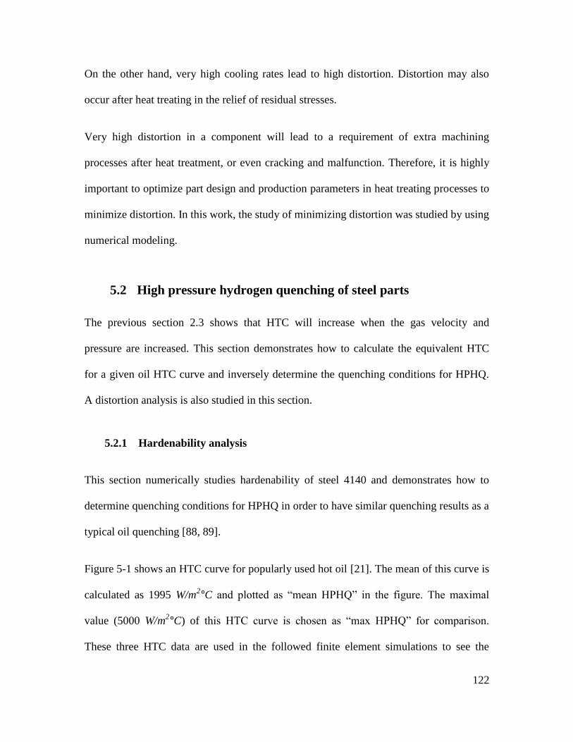
122

On the other hand, very high cooling rates lead to high distortion. Distortion may also

occur after heat treating in the relief of residual stresses.

Very high distortion in a component will lead to a requirement of extra machining

processes after heat treatment, or even cracking and malfunction. Therefore, it is highly

important to optimize part design and production parameters in heat treating processes to

minimize distortion. In this work, the study of minimizing distortion was studied by using

numerical modeling.

5.2 High pressure hydrogen quenching of steel parts

The previous section 2.3 shows that HTC will increase when the gas velocity and

pressure are increased. This section demonstrates how to calculate the equivalent HTC

for a given oil HTC curve and inversely determine the quenching conditions for HPHQ.

A distortion analysis is also studied in this section.

5.2.1 Hardenability analysis

This section numerically studies hardenability of steel 4140 and demonstrates how to

determine quenching conditions for HPHQ in order to have similar quenching results as a

typical oil quenching [88, 89].

Figure 5-1 shows an HTC curve for popularly used hot oil [21]. The mean of this curve is

calculated as 1995 W/m2°C and plotted as ―mean HPHQ‖ in the figure. The maximal

value (5000 W/m2°C) of this HTC curve is chosen as ―max HPHQ‖ for comparison.

These three HTC data are used in the followed finite element simulations to see the

123

hardenabilities. ―Mean HPHQ‖ and ―Max HPHQ‖ in this article are treated as two

quenchants like oil.

Figure 5-1. A typical oil HTC curve and its mean HTC

In this finite element simulation, a section of an infinite long cylinder shown in Figure 5-

2 is picked and meshed to analyze the cooling results from surface to the center of the

cylinder. The elements are 0.5mm in size, which is fine enough to catch the variation of

microstructure. The cylinder is made of 4140 steel with an initial microstructure of 50%

of pearlite and 50% of ferrite. The cylinder is first heated in hot furnace at 850oC for

1800 seconds for fully austenizing and cooled down in typical hot oil, ―max HPHQ‖ and

―mean HPHQ‖. The heating and cooling simulations were performed using finite element

0.00

1.00

2.00

3.00

4.00

5.00

6.00

0 200 400 600 800 1000

HTC

( kw

/m2 C

)

Work piece surface temperature ( oC )

HTC curves of different quenchants

GM hot oil

Max HPHQ

Mean HPHQ

124

package ABAQUS [10] in conjunction with DANTE [21]. DANTE is a set of user

subroutines developed for ABAQUS to govern phase transformation and material

constitutive behavior during heat treatment.

Figure 5-2. Finite element model for cooling down an infinite long cylinder

A series of simulations with cylinders varying from 25.4 mm (1 inch) to 76.2 mm (3 inch)

in diameter are conducted to compare the cooling capacities of the 3 quenchants and find

out their critical diameters. The critical diameter was first introduced by Grossmann and

was defined as the largest bar diameter that contains 50% martensite at the center after

being quenched in a given quenching media [23, 90]. Please be aware that the term

critical diameters is different from the term ideal critical diameters, which refers to the

largest bar diameter that contains 50% martensite at the center after being given an

―infinite‖ or ―ideal‖ quench. The ideal quench is one that lowers the surface temperature

of an austenized steel to the bath temperature instantaneously and therefore ideal critical

diameter is a property of a steel other than a quenchant [23].

Some of the simulation results are illustrated in Figures 5-3, 5-4 and 5-5. Figure 5-3(a)

plots the cooling curves at surface and center of the 25.4 mm diameter cylinder in a CCT

diagram of 4140 from Climax Molybdenum Company [49]. It is seen from Figure 5-3(a)

Axisymmetric surface

125

that the cooling curves do not enter to the bainite transformation zone that much and as a

result, the cylinder is through hardened with high fraction of martensite from surface to

center as shown in Figure 5-3(b). From both Figure 5-3(a) and 5-3(b), it is seen that

―mean HPHQ‖ can cool down the cylinder as fast as oil quenching.

(a) Cooling curves in CCT diagram (b) Variation of martensite

Figure 5-3. Simulation results for 25.4 mm (1 inch) diameter cylinder

Figure 5-4(a) plots the cooling curves at surface and center of the 50.8 mm diameter

cylinder in the CCT diagram of 4140. It is seen from Figure 5-4(a) that the cooling curves

enter the bainite transformation zone and as a result, high fraction of bainite and less

martensite are produced, especially at center as shown in Figure 5-4(b). From both Figure

5-4(a) and Figure 5-4(b), it is seen that ―mean HPHQ‖ can cool down the cylinder as fast

as oil quenching.

0

100

200

300

400

500

600

700

800

900

1 10 100 1000 10000 100000

Tem

pe

ratu

re (

oC

)

Time ( s )

4140 CCT

Ferrite_s

Ferrite_f

Bainite

Martensite

Oil_cen

Oil_surf

H2_max_cen

H2_mean_cen

H2_mean_surf


Temperatureat center

Temperatureat surface

90.0%

91.0%

92.0%

93.0%

94.0%

95.0%

96.0%

97.0%

98.0%

0 5 10 15

Vo

lum

e f

ract

ion


Oil-Mar%

H2_max-Mar%

H2_mean-Mar%

126

(a) Cooling curves in CCT diagram (b) Variation of martensite


(a) Cooling curves in CCT diagram (b) Phase composition of cylinder

quenched in oil

(c) Variation of martensite (d) variation of hardness


0

100

200

300

400

500

600

700

800

900

1 10 100 1000 10000 100000

Tem

per

atu

re (

o C )

Time ( s )

4140 CCT

Ferrite_s

Ferrite_f

Bainite

Martensite

Oil

Oil_surf

H2_max

H2_mean

H2_mean_surf




0.0%

10.0%

20.0%

30.0%

40.0%

50.0%

60.0%

70.0%

80.0%

90.0%

100.0%

0 5 10 15 20 25 30

Volu

me

frac

tion


Oil-Mar%

H2_max-Mar%

H2_mean-Mar%

0

100

200

300

400

500

600

700

800

900

1 10 100 1000 10000 100000

Te

mp

era

ture

( o

C )

Time ( s )

4140 CCT

Ferrite_s

Ferrite_f

Bainite

Martensite

Oil

Oil_surf

H2_max

H2_mean

H2_mean_surf




0%

10%

20%

30%

40%

50%

60%

70%

80%

90%

0 10 20 30 40

Vo

lum

e fr

acti

on


Oil-Mar%

Oil-Lbain%

Oil-Ubain%

0%

10%

20%

30%

40%

50%

60%

70%

80%

90%

100%

0 10 20 30 40

Volu

me

frac

tion


Oil-Mar%

H2_max-Mar%

H2_mean-Mar%

40

41

42

43

44

45

46

47

48

49

50

0 10 20 30 40

Har

dnes

s (H

RC)


Oil-HRC

H2_max-HRC

H2_mean-HRC

127

Figure 5-5(a) plots the cooling curves at surface and center of the 76.2 mm diameter

cylinder in the CCT diagram of 4140. From Figure 5-5(a), it is seen that the cooling

curves at surface do not enter the bainite transformation zone that much and as a result,

high fraction of martensite is produced at surface, but the cooling curves at center enter

the bainite transformation zone and less martensite is produced at center as shown in

Figure 5-5(b). Figure 5-5(c) and 5-5(d) show that variation of martensite fraction and

hardness from surface to center of the cylinder. From these figures, it is seen that ―mean

HPHQ‖ can cool down the cylinder as fast as oil quenching. Please note that magnitude

of the hardness might be different from experiments due to the accuracy of coefficients

for this steel in the phase transformation model in DANTE, but the relative difference is

reasonable [21].

It is seen that martensite fraction at center of the 50.8 mm diameter cylinder is higher

than 50% from Figure 5-6 and martensite fraction at center the 76.2 mm diameter

cylinder is less than 50% from Figure 5-6, therefore the critical diameters of this steel in

these 3 quenchants should be between 50.8 mm and 76.2 mm. Simulations of cooling

down a 56 mm (2.2 inch) diameter cylinder were performed. Figure 5-6 shows the

variation of the volume fraction of martensite at center of the cylinder with respect to

cylinder diameter. It can be seen that ―mean HPHQ‖ can quench deeper than this typical

oil.

128

Figure 5-6. Hardenability of steel 4140 in HPHQ and typical oil quenching

From the above analysis, it is seen that HPHQ with the mean of an HTC curve of a sort of

oil can produce similar results as the oil quenching. The mean HTC is 1995 W/m2°C for

this typical hot oil.

It is more important to find out the quenching condition (gas pressure and velocity) of

HPHQ to generate such a mean HTC. The conditions to generate such a mean HTC are

inversely determined from Equation 11. From the definition, Prandtl number is a constant

for a given gas and Nusselt number is a constant if HTC is fixed (as 1995 W/m2°C in this

case), therefore the gas pressure (density) and velocity can be determined by solving the

non-linear equation of Reynolds number. Newton iteration method is applied to solve this

non-linear equation and therefore the quenching conditions for HPHQ are determined and

plotted in Figure 5-7. HPHQ at 20 bar and 20 m/s will meet the requirement. The

counterpoints for helium and nitrogen are also determined and plotted in Figure 5-7. It is

0%

25%

50%

75%

100%

0 20 40 60 80

Vo

lum

e fr

acti

on

Cylinder diameter (mm)

Martensite vs. diameter

Dante oil

hydrogen max

hydrogen mean

56mm

129

seen that hydrogen requires lower pressure or velocity than helium and nitrogen to

generate the mean HTC.

Figure 5-7. Conditions of HPHQ for the equivalent HTC

5.2.2 Distortion Analysis

Since HTC around a work piece is not uniform and HTC distributions for different

orientations are different, it is worthy to study the differences of distortion for different

HTC distributions and find out the optimal part orientation when the distortion of a target

portion of a part is minimized. This section studies the effect of HTC distribution on

distortion of a ring shown in Figure 5-8 and compares the distortion of the inner circle

when quenched at different orientations shown in Figure 5-9 [89, 91]. The ring is made of

4140 steel.

130

Figure 5-8. Schematic drawing of a ring (unit in mm)

Figure 5-9. Directions of gas flow

In this work, CFD simulations were conducted to obtain hydrogen flow and HTC

distribution. Figure 5-9 shows a half ring in the middle of the gas domain since this is a

symmetric problem. The environment pressure is set as 15 bar and inlet gas velocity is set

as 21 m/s. The inlet hydrogen temperature is 25 oC and the initial ring temperature is

850oC. K-epsilon turbulence model is applied in the CFD simulation. The HTC

distribution from CFD simulation ranges from about 900 to 2500 CmW o2/ , as illustrated

in Figure 5-11. In gas quenching, the HTC data for front faces are usually smaller than

Ø50.8Ø25.4

9.5

3.2

0°

30°

60°90°

150°

120°

180°

131

other faces because the local gas velocities near front faces are usually very small or even

zero at some locations. The average HTC in this case is about 1950 CmW o2/ .

Figure 5-10. CFD modeling for distributed HTC

Figure 5-11. HTC distribution for 0 degree gas flow

The node-based HTC distributions obtained from CFD simulations are mapped to finite

element models. Because the distortion of the inner circle is studied, one point of the

inner circle is fixed to remove free body movement as shown in Figure 5-12. In this case,

the distortion or the shape of the inner circle after quenching can be compared easier. In

the finite element simulations using ABAQUS [10], DANTE [21] is applied to model

Gas domain

Half ring

Direction :180o

Direction: 0o

HTC (W/m2 oC)

132

phase transformation and material constitutive behavior of steel 4140 in the quenching

process. In the ABAQUS models, there are 4305 nodes and 3360 elements. The elements

are about 3 mm in size.

Figure 5-12. Finite element modeling

Figure 5-13 shows the distortion of the ring after quenching at two different orientations

with a scale factor of 100. It shows clearly that distortion at different orientations is

different. In other words, the HTC distribution plays a very big important role in

generating distortion.

(a) Distortion of the ring for 0 degree flow

H2

flow

133

(b) Distortion of the ring for 180 degree

Figure 5-13. Distortion of the ring at different orientation (mm)

The shapes of the inner circle after quenching at different orientations were calculated by

adding scaled displacements in the circle plane of nodes of the path (red line in Figure 5-

12) by 100 times to the original shape and plotted in Figure 5-14. The solid blue line was

the original shape and other shapes after quenching were scaled up 100 times for a clearer

view. The out of roundness values of the inner circle were also calculated approximately

and illustrated in Figure 5-15. In the approximate calculation, the displacement in the

circle plane of each node of the path was treated as the change of radius. The change of

radius was assigned positive or negative symbol according to the displacement direction.

The out of roundness was determined as the difference between maximum and minimum

changes of radius. The figures show clearly that the distortion for each orientation is

different and implies that:

(a) For a specific portion of a part, uniform-in-space HTC data do not necessarily

produce the best results. In this case, the shapes using uniform-in-space HTC labeled as

h2_avg and oil is even worse than the shapes at 0 degree and 90 degree.

H2 flow

134

(b) For this ring, 0, 30 and 90 degree flows generate the lowest distortion of the inner

circle. It should be chosen for production if the distortion of the inner circle must be

minimized.

(c) It should be noted that 0, 30 and 90 degree flows might not produce the best results

for other portion of the part. The best orientation may be determined after comparing

distortions of all critical portions of the part.

Figure 5-14. Comparison of scaled shapes of inner circle

Figure 5-15. Approximation of out of roundness of the inner circle

0

2

4

6

8

10

12

14

-5 0 5 10 15 20 25 30

Y (

mm

)

X (mm)

Scaled Shapes of Inner Circle Original

Oil

H2_avg

CFD (0o)

CFD (30o)

CFD (60o)

CFD (90o)

CFD (120o)

CFD (150o)

CFD (180o)

Scale Factor=100

Oil, 0.0478

H2_avg, 0.0320

(0 ), 0.0146 (30 ), 0.0153

(60 ), 0.0424

(90 ), 0.0144

(120 ), 0.0725

(150 ), 0.0673

(180 ), 0.0350

0

0.01

0.02

0.03

0.04

0.05

0.06

0.07

0.08

Approximation of out of roundness (mm)

135

5.3 Summary

In this work, a few numerical simulations of high pressure hydrogen quenching of steel

components using finite element package ABAQUS and a user subroutine set DANTE

were conducted. A hardenability analysis of a steel rod was conducted to compare the

quenching severity of HPHQ and oil quenching from the points of view of microstructure

and hardness. This analysis indicates that HPHQ with an HTC value at the mean level of

the HTC curve for a typical oil quenching can produce similar microstructure as the oil

quenching. A study was also made on the HTC distribution effect on distortion of a steel

ring. This study shows that distortions of the same component at different quenching

orientation are different and implies that distortion can be minimized by choosing a

proper orientation. It is also illustrated that distortion of the component is lower than oil

quenching when similar microstructure is produced in the two quenching processes.

136

6 Conclusion and potential applications in other areas

This chapter concludes the numerical modeling and experimental investigation of various

quenching processes and points out the potential application of the numerical models

developed in this work.

6.1 Conclusions

In this work, the problems and challenges in numerical modeling of gas and liquid

quenching processes were analyzed and models were developed to solve the key issues in

the numerical simulations.

1. In the heat transfer modeling chapter, four existing methods to determine thermal

boundary condition, HTC distribution, for solid components in quenchant flow were

analyzed and applied in gas and liquid quenching processes. These methods include

empirical equation method, lumped heat capacity method, CFD simulation method and

iterative modification method. Two new methods were developed to determine the HTC

distribution at high accuracy and low cost. The first developed method, called semi-

empirical equation method, was established based on experimental investigation. At the

end, another new method, integrating CFD simulation method, iterative modification

method and semi-empirical equation method together, was developed to determine node-

based HTC distributions for complicated components at very high accuracy. A US patent

was filled for this new method with General Motors Company. A valuable HTC database

for air quenching and water quenching was also built and validated.

137

2. In the material property evolution modeling chapter, material property evolution

of steel and aluminum alloy parts were addressed. The variations of their constitutive

behaviors lead to the need of development of user material constitutive subroutines in

finite element simulations. The commercially available user material subroutine set,

DANTE, was applied with finite element package ABAQUS for simulation of quenching

of steel components. The material property evolution of aluminum alloy castings during

quenching was also analyzed and a user material constitutive subroutine was developed

based on a particular constitutive model that governs the stress-strain behavior during

quenching. An extended framework was also proposed in this work to account for the

possible aging effect during quenching and to simulate the aging process.

3. In the residual stress prediction and measurement chapter, residual stresses in

quenched aluminum alloy and steel components were predicted by applying the heat

transfer and material constitutive models, and compared to experimental measurements

using mainly resistance strain gauge rosette hole-drilling method. Improvement for this

measurement method was proposed for higher accuracy and validated by experimental

investigation. Residual stresses were predicted in the quenching cases: water quenching

of an aluminum alloy frame-shape casting, water quenching of an aluminum alloy

cylinder head, air quenching of an aluminum alloy frame-shape casting and air quenching

of an aluminum alloy engine block. Good agreements of residual stresses in the quenched

components between predictions and experimental measurements validate the numerical

simulation procedure and the numerical models developed in this work.

4. In the numerical comparisons between gas and liquid quenching chapter, a

hardenability analysis and a distortion study were conducted for high pressure hydrogen

138

quenching and typical oil quenching of steel components. The hardenability study shows

that high pressure hydrogen quenching with HTC data at the mean level of an HTC curve

of oil quenching will produce similar microstructure (martensite volume fraction, etc.)

and hardness to what the oil quenching produces. The distortion study indicates that

distortion of a steel component in high pressure hydrogen quenching is lower than that in

oil quenching when similar microstructures are produced. This study also shows

distortions at different quenching orientations are different, which implies that distortion

can be minimized by choosing a proper quenching orientation.

6.2 Potential applications in other areas

In this work, the numerical models were developed and applied for quenching processes,

but they can also be applied in other situations where temperature, stress and distortion

are involved.

A. The numerical models can be applied in other heat treating processes such as

annealing, tempering, aging, etc.

For instance, in the steel tempering process, the methods developed in this work to

determine HTC distribution for any part can be applied to predict temperature-time

profile. The material property evolution model for steel can be applied to govern the

phase transformation and constitutive behavior, which in conjunction with finite element

package can predict the generation of distortion, stress and strain.

B. The numerical models can be applied in other manufacturing processes such as

welding, casting, etc.

139

For instance, in the welding process, the parts are heated up and then cooled down. The

heat transfer modeling and material property evolution modeling can be applied to predict

the temperature profile, phase transformation, stress profile, etc.

C. The numerical models can be applied in other industries such as new energy

industry, semi-conductor industry, etc.

For instance, in the new energy industry, solar panels and their mounting systems

experience temperature variation during usage due to the air temperature change in

seasons and the heat from sun. As a result, thermal expansion introduces reliability and

deformation problems. The models developed in this work governing thermal and

material behavior can be applied in such situations.

Applying the models to the thermal management of electronic systems such as laptop is

another example. In this case, the design of the cooling system (fan speed, configuration,

etc) strongly depends on heat transfer coefficient, which is well addressed and can be

determined with the models in this work.

140

7 References

[1] Elgun, S. Z., 1999, "TTT Diagram,"

Http://info.Lu.Farmingdale.edu/depts/met/met205/tttdiagram.Html, 2009(12/2) .

[2] Elkatatny, I., Morsi, Y., Blicblau, A. S., 2003, "Numerical Analysis and Experimental

Validation of High Pressure Gas Quenching," International Journal of Thermal Sciences,

42(4) pp. 417-423.

[3] Rose, A., Kessler, O., Hoffmann, F., 2006, "Quenching Distortion of Aluminum

Castings-Improvement by Gas Cooling," Materialwissenschaft Und Werkstofftechnik,

37(1) pp. 116-121.

[4] Li, P., Maijer, D. M., Lindley, T. C., 2007, "Simulating the Residual Stress in an

A356 Automotive Wheel and its Impact on Fatigue Life," Metallurgical and Materials

Transactions B, 38(4) pp. 505-515.

[5] Li, K., Xiao, B., and Wang, Q., 2009, "Residual Stresses in as-Quenched Aluminum

Castings," SAE International Journal of Materials & Manufacturing, 1(1) pp. 725-731.

[6] Li, M., and Allison, J. E., 2007, "Determination of Thermal Boundary Conditions for

the Casting and Quenching Process with the Optimization Tool OptCast," Metallurgical

and Materials Transactions B, 38B(4) pp. 567-574.

http://info.lu.farmingdale.edu/depts/met/met205/tttdiagram.Html

141

[7] Xiao, B., Rong, Y., and Li, k., 2010, "Residual Stresses in Water and Air Quenched

Aluminum Alloy Castings," Proceedings of SEM Annual Conference & Exposition on

Experimental and Applied Mechanics 2010, Society for Experimental Mechanics Inc., .

[8] Lee, Y.L., Pan, J., Hathaway, R., 2005, "Fatigue testing and analysis: theory and

practice," Elsevier Butterworth-Heinemann, pp. 402.

[9] Kibey, S., Sehitoglu, H., and Pecknold, D. A., 2004, "Modeling of Fatigue Crack

Closure in Inclined and Deflected Cracks," International Journal of Fracture, 129(3) pp.

279-308.

[10] ABAQUS, I., 2007, "ABAQUS Help Documentation," 6.7.

[11] ANSYS, I., 2009, "ANSYS Documentation," 12.1.

[12] Li, Z., Grandhi, R. V., and Srinivasan, R., 2006, "Distortion Minimization during

Gas Quenching Process," Journal of Materials Processing Technology, 172(2) pp. 249(9).

[13] Holman, J.P., 2002, "Heat Transfer," McGraw-Hill, New York, pp. 665.

[14] Sedighi, M., and McMahon, C. A., 2000, "The Influence of Quenchant Agitation on

the Heat Transfer Coefficient and Residual Stress Development in the Quenching of

Steels," Proceedings of the Institution of Mechanical Engineers, Part B: Journal of

Engineering Manufacture, 214(7) pp. 555-567.

142

[15] Newman, M. L., Robinson, B. J., Sehitoglu, H., 2003, "Deformation, Residual Stress,

and Constitutive Relations for Quenched W319 Aluminum," Metallurgical and Materials

Transactions A, 34(7) pp. 1483-1491.

[16] Sehitoglu, H., Smith, T., Qing, X., 2000, "Stress-Strain Response of a Cast 319-T6

Aluminum Under Thermomechanical Loading," Metallurgical and Materials


[17] Estey, C. M., Cockcroft, S. L., Maijer, D. M., 2004, "Constitutive Behaviour of

A356 during the Quenching Operation," Materials Science & Engineering A, 383(2) pp.

245-251.

[18] Lu, J., and James, M., 1996, "Handbook of measurement of residual stresses,"

Fairmont Press,Inc, Lilburn, GA, USA, pp. 237.

[19] Schajer, G. S., 1988, "Measurement of Non-Uniform Residual Stresses using the

Hole-Drilling Method. Part I-Stress Calculation Procedures," Journal of Engineering

Materials and Technology, 110pp. 338-343.

[20] ASTM designation: E837-01, 2002, ASTM international, Philadelphia, PA, pp. 703-

712.

[21] Deformation Control Technology, I., 2008, "DANTE Heat Treatment Simulation

Software Help," 3.3.

143

[22] Li, H., Zhao, G., Niu, S., 2007, "Technologic Parameter Optimization of Gas

Quenching Process using Response Surface Method," Computational Materials Science,

38(4) pp. 561-570.

[23] Totten, G.E., Bates, C.E., and Clinton, N.A., 1993, "Handbook of quenchants and

quenching technology," ASM International, Materials Park, OH, pp. 514.

[24] Giacobbe, F., 1998, "Heat Transfer Capability of Selected Binary Gaseous Mixtures

Relative to Helium and Hydrogen," Applied Thermal Engineering, 18(3-4) pp. 199-206.

[25] Churchill, S., and Bernstein, M., 1977, "A Correlating Equation for Forced

Convection from Gases and Liquids to a Circular Cylinder in Crossflow," ASME,

Transactions, Series C-Journal of Heat Transfer, 99pp. 300-306.

[26] Faura, F., Campo, A., and Zamora, B., 1998, "A Mixture of Pure Gases that Produce

Maximum Heat Transfer Characteristics for Quenching," Journal of Materials

Engineering and Performance, 7(3) pp. 420-424.

[27] Innovative Nuclear Space Power and Propulsion Institute, "Hydrogen Properties

Package," Http://www.Inspi.Ufl.edu/data/h_prop_package.Html, 2009(May 15) .

[28] The National Institute of Standards and Technology, "Thermophysical Properties of

Hydrogen," Http://www.Boulder.Nist.gov/div838/Hydrogen/Properties/Properties.Htm,

2009(May 15) .

http://www.inspi.ufl.edu/data/h_prop_package.Html

http://www.boulder.nist.gov/div838/Hydrogen/Properties/Properties.Htm

144

[29] The engineering toolbox, 2005, "The Engineering Toolbox,"

Http://www.Engineeringtoolbox.com/nitrogen-d_1421.Html, 2009(5/15) .

[30] Laumen, C., Midea, S. I., Lubben, T., 1997, "Measured heat transfer coefficients by

using hydrogen as quenchant in comparison with helium and nitrogen," Accelerated

Cooling/Direct Quenching of Steels, Indianapolis, Indiana; USA;, pp. 199-206.

[31] Chaffotte, F., Domergue, D., Kazi, S., 2005, "Optimizing Gas Quenching

Technology through Modeling of Heat Transfer," Industrial Heating, 72(11) pp. 49-53.

[32] Sugianto, A., Narazaki, M., Kogawara, M., 2008, "A Comparative Study on

Determination Method of Heat Transfer Coefficient using Inverse Heat Transfer and

Iterative Modification," Journal of Materials Processing Technology, 209(10) pp. 4627-

4632.

[33] Maniruzzaman, M., Chaves, J., McGee, C., 2002, "CHTE Quench Probe System: A

New Quenchant Characterization System," 5th International Conference on Frontiers of

Design and Manufacturing (ICFDM), pp. 619-625.

[34] Funatani, D. K., Narazaki, M., and Tanaka, M., 1999, "Comparisons of Probe

Design and Cooling Curve Analysis Methods," 19th ASM heat treating society

conference proceedings including steel heat treating in the new millennium, G. Krauss, S.

J. Midea and G. D. Pfaffmann, eds. ASM international, Cincinnati, Ohio, pp. 255-263.

http://www.engineeringtoolbox.com/nitrogen-d_1421.Html

145

[35] Kobasko, N. I., Moskalenko, A. A., Totten, G. E., 1997, "Experimental

Determination of the First and Second Critical Heat Flux Densities and Quench Process

Characterization," Journal of Materials Engineering and Performance, 6(1) pp. 93-101.

[36] Mills, A.F., 1995, "Heat and mass transfer," CRC Press, Irwin, MA, USA, pp. 1280.

[37] The MathWorks, I., 2007, "MATLAB Help Documentation," The MathWorks, Inc,

2007B.

[38] Python Software Foundation, 2008, "Python Documentation," Http://python.org/doc/,

2.5.

[39] Gerald P. Backer, 1998, "Computer-Aided Engineering Software for Semi-Solid

Metal Manufacturing," JOM Journal of the Minerals, Metals and Materials Society, 50(8)

pp. 21-23.

[40] Scientific Forming Technologies Corporation, 2007, "DEFORM Decoumentation,"

Http://www.Deform.com/products/deform-ht/ht-Brochure.Pdf, .

[41] Dassault Systèmes, 2008, "Isight," 3.5.

[42] ASM International Handbook Committee, 1991, "ASM Handbook," ASM

International, Metals Park, OH, pp. 448.

[43] Kim, J., "Review of Nucleate Pool Boiling Bubble Heat Transfer Mechanisms,"

International Journal of Multiphase Flow, In Press, Accepted Manuscript.

http://python.org/doc/

http://www.deform.com/products/deform-ht/ht-Brochure.Pdf

146

[44] GM Powertrain, 2002, "temperature-time curves of Gen V8 block," GM Powertrain.

[45] ANSYS Inc., 2009, "ANSYS Fluent Documentation," 12.1.

[46] ANSYS Inc., 2009, "ANSYS CFX Documentation," 12.1.

[47] Wang, G., Xiao, B., Zhang, L., 2008, "Heat Transfer Coefficient Study for Air

Quenching by Experiment and CFD Modeling," 137th Annual Meeting & Exhibition.

Materials Characterization, Computation and Modeling, TMS (The Minerals, Metals &

Materials Society), Warrendale, PA, USA, 2, pp. 271-276.

[48] Wang, Q., Xiao, B., Wang, G., 2010, "Systems and Methods for Predicting Heat

Transfer Coefficients during Quenching," (pending patent) .

[49] Cias, W.W., 1977, "Austenite transformation kinetics of ferrous alloys," NP-23519,

Climax Molybdenum Co., Greenwich, CT, pp. 83.

[50] Polmear, I.J., 1995, "Light Alloys:Metallurgy of the Light Metals," Butterworth-

Heinemann, London, UK, pp. 384.

[51] Lorimer, G. W., 1978, "Precipitation Processes in Solids," Proceedings of a

symposium sponsored by the TMS-AIME Heat Treatment Committee, K. C. Russell and

H. I. Aaronson, eds. Metallurgical Society of AIME, pp. 87.

[52] Porter, D.A., and Easterling, K.E., 2000, "Phase transformations in metals and

alloys," Stanley Thornes Ltd, Cheltenham, UK, pp. 514.

147

[53] Kavalco, P. M., Canale, L. C. F., and Totten, G. E., 2009, "Quenching of Aluminum

Alloys:Cooling Rate, Strength, and Integranular Corrosion," Heat Treating Progress, 9(7)

pp. 25-30.

[54] Croucher, T., 1982, "Quenching of Aluminum Alloy:What this Key Step

Accomplishes," Heat Treating, 14(5) pp. 20-21.

[55] Silcock, J. M., Heal, T. J., and Hardy, H. K., 1953, "Structural Ageing

Characteristics of Binary aluminium–copper Alloys," J.Inst.Met, 82pp. 239-248.

[56] Sanpaz, 2009, "FileStress Transformation 3D_svg - Wikipedia, the Free

Encyclopedia.Mht," Http://en.Wikipedia.org/wiki/File:Stress_transformation_3D.Svg,

2010(January 13) .

[57] Ugural, A.C., and Fenster, S.K., 1995, "Advanced strength and applied elasticity,"

Prentice-Hall, New Jersey, pp. 539.

[58] Lu, Y., and Zhou, Z., 2002, "Finite Element Analysis of Mechanical and Automobile

Structure," Tongji University, Shanghai, China, pp. 186.

[59] Henriksen, M., Larson, D. B., and Van Tyne, C. J., 1992, "On the Analysis of

Distortion and Residual Stress in Carburized Steels," Journal of Engineering Materials

and Technology, 114pp. 362.

[60] Lusk, M., Krauss, G., and Jou, H. J., 1995, "A Balance Principle Approach for

Modeling Phase Transformation Kinetics," Journal De Physique IV, 5(8) pp. 279-286.

http://en.wikipedia.org/wiki/File:Stress_transformation_3D.Svg

148

[61] Lee, Y. K., and Lusk, M. T., 1999, "Thermodynamic Prediction of the Eutectoid

Transformation Temperatures of Low-Alloy Steels," Metallurgical and Materials


[62] Lee, S. J., Lusk, M., and Lee, Y. K., 2007, "Conversional Model of Transformation

Strain to Phase Fraction in Low Alloy Steels," Acta Materialia, 55(3) pp. 875-882.

[63] Lusk, M. T., and Lee, Y. K., 1999, "A global material model for simulating the

transformation kinetics of low alloy steels," Heat Treatment and Surface Engineering of

Light Alloys, Proceedings of the 7th Int. Seminar of IFHT, Budapest, Hungary,

September, pp. 15-17.

[64] Lusk, M. T., Jaramillo, R., Roche, A., "Microstructural Evolution in Sprayformed

Steel: Phase Transitions, Inelasticity, Residual Stress and Distortion," Microstructural

Modeling and Prediction during Thermomechanical Processing, pp. 75–84.

[65] Speer, J., Matlock, D. K., Cooman, B. C. D., 2003, "Carbon Partitioning into

Austenite After Martensite Transformation," Acta Materialia, 51(9) pp. 2611.

[66] Prantil, V., Callabresi, M., Lathrop, J., 2003, "Simulating Distortion and Residual

Stresses in Carburized Thin Strips," Journal of Engineering Materials and Technology,

125pp. 116.

[67] Sehitoglu, H., and Karasek, M., 1986, "Observations of Material Behavior Under

Isothermal and Thermo-Mechanical Loading," Journal of Engineering Materials and

Technology, 108(2) pp. 192-198.

149

[68] Jiang, Y., and Sehitoglu, H., 1996, "Modeling of Cyclic Ratchetting Plasticity, Part I:

Development of Constitutive Relations," Journal of Applied Mechanics, 63pp. 720.

[69] Jiang, Y., and Sehitoglu, H., 1996, "Modeling of Cyclic Ratchetting Plasticity, Part

II: Comparison of Model Simulations with Experiments," Journal of Applied Mechanics,

63pp. 726.

[70] Sehitoglu, H., 1989, "Changes in State Variables at Elevated Temperatures," Journal

of Engineering Materials and Technology, 111(2) pp. 192-203.

[71] Karaman, I., Balzer, M., Sehitoglu, H., 1998, "Stress-State Effects on the Stress-

Induced Martensitic Transformation of Carburized 4320 Steels," Metallurgical and

Materials Transactions A, 29(2) pp. 427-437.

[72] Compaq, I., 2002, "Fortran," 6.6.

[73] Simo, J.C., and Hughes, T.J.R., 2000, "Computational inelasticity," Springer, pp.

392.

[74] Smith, T. J., Sehitoglu, H., Fleury, E., 1999, "Modeling High-Temperature Stress-

Strain Behavior of Cast Aluminum Alloys," Metallurgical and Materials Transactions A,

30(1) pp. 133-146.

[75] Sisson Jr, R.D., Backman, D., Maniruzzaman, M., 2007, "Aging cycle optimization

for aluminum alloys," CHTE project report, 07-01, Worcester, MA.

150

[76] Sisson Jr, R.D., Backman, D., Maniruzzaman, M., 2008, "Aging cycle optimization

for aluminum alloys," CHTE project, 08-02, Worcester, MA.

[77] Vishaymicro-Measurements, 2007, "Tech Note TN-503:Measurement of Residual

Stresses by the Hole-Drilling Strain Gage Method," 2009pp. 33.

[78] Schajer, G. S., 1988, "Measurement of Non-Uniform Residual Stresses using the

Hole-Drilling Method. Part II-Practical Application of the Integral Method," Journal of

Engineering Materials and Technology, 110pp. 344-349.

[79] Li, K., 1995, "Interferometric 45 and 60 Strain Rosettes," Applied Optics, 34(28) pp.

6376-6379.

[80] Tjhung, T., and Li, K., 1999, "On accuracy of residual stress measurements by hole-

drilling and interferometric strain rosette," Proceedings of the SEM Annual Conference

on Theoretical, Experimental and Computational Mechanics, Society for Experimental

Mechanics, Inc, pp. 387-390.

[81] Li, K., and Ren, W., 2007, "Application of Minature Ring-Core and Interferometric

Strain/Slope Rosette to Determine Residual Stress Distribution with Depth—Part I:

Theories," Journal of Applied Mechanics, 74pp. 298.

[82] Bragg, W. L., 1912, "The diffraction of short electromagnetic waves by a crystal,"

Proceedings of the Cambridge Philosophical Society, 17, pp. 43-57.

151

[83] Wikimedia Foundation Inc., 2009, "Bragg's Law - Wikipedia, the Free

Encyclopedia.Mht," Http://en.Wikipedia.org/wiki/Bragg's_law#cite_note-0,

2009(December 15) .

[84] Xiao, B., Li, K., and Rong, Y., 2010, "Automatic Determination and Experimental

Evaluation of Residual Stress Calibration Coefficients for Hole-Drilling Strain Gage

Integral Method," Strain, In Press, Accepted Manuscript.

[85] H Wern, 1995, "Measurement of Non-Uniform Residual Stresses using the Hole

Drilling Method, a New Integral Formalism," Strain, 31(2) pp. 63-68.

[86] Crawford, M., and Werner, J., 2004-2006, "GM Power train Evaluation reports on

residuals tress measurement of GEN IV," Pontiac, MI, USA.

[87] Bell, T., 1972, "Survey of the Heat Treatment of Engineering Components,"

I.S.I.Monograph, 56pp. 106.

[88] Xiao, B., Wang, G., and Rong, Y., 2009, "A Study on Heat Transfer Coefficient of

High Pressure Hydrogen Quenching," Heat Treating: Proceedings of the 25th ASM Heat

Treating Society Conference, F. Specht, S. MacKenzie and D. Weires, eds. ASM

International, pp. 101-104.

[89] Xiao, B., Wang, G., and Rong, Y., 2010, "Hardenability and Distortion Control in

High Pressure Hydrogen Quenching," International Journal of Manufacturing Research,

In press, accepted manuscript.

http://en.wikipedia.org/wiki/Bragg's_law#cite_note-0

152

[90] Grossmann, M.A., 1952, "Elements of hardenability," American Society for Metals,

Cleveland, OH, pp. 146.

[91] Xiao, B., Wang, G., and Rong, Y., 2010, "A Study on Heat Transfer Coefficient

Distribution in High Pressure Hydrogen Quenching," Proceedings of 139th TMS annual

meeting & exhibition, TMS (The Minerals, Metals & Materials Society), Warrendale,

PA, USA, 1, pp. 479-486.

Figure 2-10.

Documents

Transcript of Figure 2-10.