Fifth Draft Dick - anderson.ucla.edu

The End of Class Warfare, April 20, 2002

1

The End of Class Warfare: An Examination of Income Disparity

by

Richard Roll and John Talbott*

April 20, 2002

Abstract

During the 1990s, the richest quintile of a country had an average income per capita approximately ten times that of the poorest quintile. We find that the poor of a country are better off relatively, and absolutely, when the country ranks higher in average income, union participation, taxation, government spending, education, and property rights. Under these same conditions, the wealthy of a country also have more absolute per capita income, just not a higher percentage relative to the poor. Countries with substantial black market activity, high levels of international trade (as a percentage of GDP), and former Spanish colonies have greater income disparity; these features also coincide with lower incomes for both rich and poor. Key features of democracy such as political and voting rights, civil liberties and freedom of the press, while important for economic growth, are not independently associated with income inequality. We find little empirical support for a tradeoff between a high level of prosperity and greater equality. Above a very low level of development, appropriate policies are associated with both higher average and more equal income.

Roll Talbott

Address Anderson School, UCLA 110 Westwood Plaza Los Angeles, CA 90095-1481

Global Development Group 2260 El Cajon Boulevard, #201 San Diego, CA 92104

Voice 310-825-6118 619-772-3849 Fax 310-206-8404 619-295-5036

E-Mail [email protected] [email protected] * The authors thank The Heritage Foundation, the World Bank, Freedom House and the International Labor Organization for years of data compilation that make empirical research a possibility. We also thank Daron Acemoglu for patiently explaining his recent work on institutions and development. We deeply appreciate the hard work by the reference librarians at UCSD, whose selfless effort can only be compensated by this short mention of gratitude.


2

The End of Class Warfare

An Examination of Income Disparity

The cries of “Free Markets!” screamed out by the striking union workers were drowned out by the shouts of “Higher Wages!” from the factory owner and her husband. ------A possible storyline from a newspaper in the year 2020.

I. Introduction

Most studies of inequality within countries have focused on the percentages of income

received by various income quantiles, or else on Gini coefficients.1 But if one seeks to

alleviate poverty, perhaps a better gauge of success would be the per capita income of the

poor. An effective policy would make the poor richer while having a positive or neutral affect

on the rest of the population. Only average income levels by quantile, not percentages, can

reveal such an effect.

In this paper, we study a broad geographic mix of developing and developed countries. On

average in our sample of 113 countries, the poorest quintile earns 6.4% of total country

income, while the richest quintile earns 46.7% of the total. The average country’s ratio of the

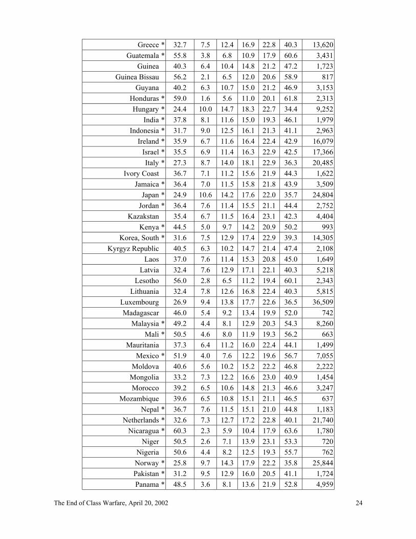
two is 9.8. Table 1 presents the sample of countries along with inequality and income

measures. These data cover a period from 1991 through 1996 inclusive. It is impossible to

better align the data temporally across nations because inequality measures are based on

surveys that occur infrequently at different times in different countries. Pertinent details are

available on the internet at the websites of the individual sources.

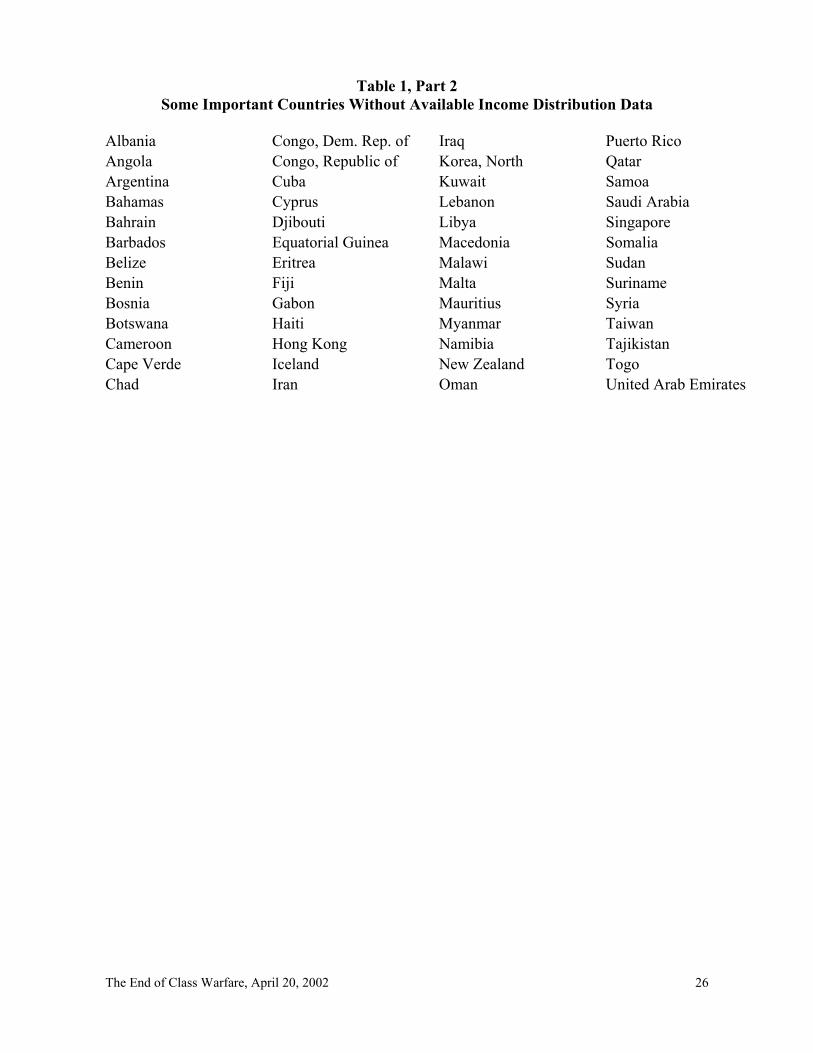
Although the sample appears to cover a wide range of country incomes, we recognize it could

be biased. The very poorest nations are less apt to report statistics of any kind and perhaps are

even more reluctant to reveal income inequality figures. Other countries, even when

relatively rich, might be embarrassed to report dramatic inequality. Table 1 names 56

countries for which we have no income distribution data. With a few inexplicable exceptions

(Iceland, New Zealand), and a few others that may not care to reveal income distributions for

their own reasons (Kuwait, Taiwan), most are poor and several are among the poorest on the

1 See Appendix A for a description of the Gini coefficient.


3

planet. We hope their exclusion has simply lessened the likelihood of uncovering statistically

significant results and has not brought an incorrect inference, but we are unable to provide

any assurance and can only plead that it would be entirely unintentional.

We examine 21 different potential determinants of inequality, measuring their relation with

Gini coefficients, income percentages by quintile and average dollar incomes per capita by

quintile. Table 2 lists and describes them. Multicollinearity among these variables can be

overcome with appropriate empirical methods, but the more serious conceptual problem of

endogeneity cannot be; hence, conclusions about causality remain unavoidably ambiguous.

In general, richer countries tend to have more egalitarian distributions of income. Only five

of the 113 countries in our sample had both above-average inequality, (as measured by the

Gini coefficient), and above-average income per capita.2 Countries that are richer, or have

higher union participation, more extensive education systems, stronger property rights, higher

taxes, or more government spending are more egalitarian. Somewhat surprisingly, among

these factors associated with greater equality, almost none has a damaging effect on the

wealthy as measured by average income per capita for the richest quintile.

Black market activity, international trade (as a percentage of GDP) or being a former Spanish

colony is each associated with greater inequality. Although democratic institutions nurture

development and growth (Roll and Talbott [2001]), they are not significantly associated with

inequality, once the average level of income is taken into account. Of course since greater

wealth is associated with more equality, democratic institutions might have an indirect

positive egalitarian influence.

If the factors we measure really are causes and not the effects of greater equality, then policies

are available to both stimulate growth and diminish income disparity. These goals do not

seem to be mutually exclusive.

2 These countries were Chile, Malaysia, South Africa, Uruguay, and the United States.


4

II. The Issues and Some Preliminary Empirical Results.

Journalists and politicians frequently suppose that income redistribution is a zero-sum game;

i.e., any action taken to help one class hurts another. Such a conclusion is, in fact, inescapable

if redistribution is measured by the percentages of income accruing to various wealth groups.

By construction, percentages must aggregate to 100%, so if the poorest quintile’s percentage

increases, at least some richer quintile percentage must decrease.

But such arithmetic ignores the absolute income level of each class, which is perhaps more

relevant. To see the difference, think about the following choice: would one rather be a poor

citizen of a country where the poorest quintile earns five percent of the total income and the

average per capita income is $10,000, or a poor citizen of a country where the poorest quintile

earns ten percent of the total income and average per capita income is $1,000? The average

poor citizen in the first country has five times the income of the average poor citizen in the

second. Unless envy of richer fellow citizens is an overweening sentiment, few would prefer

the second alternative.

Across the 113 countries in our sample, the ratio of high to low quintile income percentage

ranges from 2.6 to 57.6. Considering such proportions, an understandable gut reaction for

improving the lot of the poor is simply to transfer resources from the rich. By transferring

6.4% of total income from the richest quintile to the poorest, the poor incomes would double

while the wealthiest incomes would still exceed 40% of the total. A relatively small burden

on the rich can appear to loom large in the alleviation of suffering.

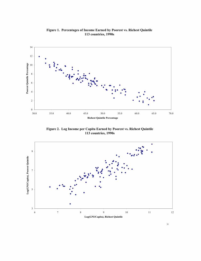
A cross-country comparison of income percentages reveals the empirical extent of this

apparent tradeoff. Figure 1 plots the lowest quintile (LQ) income percentage against the

highest quintile (HQ) income percentage for our 113 countries.3 This certainly looks like a

zero-sum game and a casual empiricist might be forgiven for that deduction. Consider,

though, that the scatter in Figure 1 is not perfectly co-linear entirely because the three middle

quintiles have been ignored. There would be a perfect relation between the percentage in any

fractile of the distribution and its compliment.

3 No figure in this paper necessarily implies causality running from the x-axis variable to the y-axis variable.


5

Instead of using percentages, we might employ the same underlying data to compare average

dollar incomes per capita in various quintiles. If Gi is average income per capita (GNI/Capita)

for country i, Ni is the population, and πij is the percentage that quintile j receives in country i,

then the per capita average income of quintile j in country i is gij=(πijGiNi)/(Ni/5)=5πijGi.4

Figure 2 plots, across the same countries used in Figure 1, the lowest quintile versus the

highest quintile average incomes per capita.

The results are striking. Based on incomes rather than percentages, there is a strong positive

cross-country correlation between the poorest and richest quintile incomes. Not only is there

no evidence of a trade-off between rich and poor; the casual empiricist might readily conclude

from Figure 2 that the goose and the gander have coincidental interests.

Moving beyond bivariate comparisons of income class percentages complicates the study of

inequality. As we shall see, a number of different factors are related to inequality, but

causality directions are problematic and multicollinearity is extensive among possible

determinants. It is tempting to predict that particular policies will benefit one class, while

harming another. Yet there could be unforeseen and unintended consequences. To this point,

we do not even know whether policies intended to reduce income disparity actually deliver

resources to the poor, nor whether they have any impact whatsoever on the rich or on the

average citizen.

4 This calculation assumes that the pre-tax total GNI is distributed according to the measured quintile fractions, which were essentially based on after-tax consumption. Later, we will examine the implications of this assumption.


6

III. Inequality and Its Proximate Determinants.

Figure 3 plots Gini coefficients against average GNI/capita across our sample of countries.

High income is associated with low Gini values and hence more equality. What is most

interesting is not where the data points lie in this figure, but rather where they do not. The

upper right hand quadrant is virtually empty. Only a few countries in our sample have both

above-average income and above-average inequality.

Following Kuznets [1955], previous researchers (Ahluwalia, [1976], Jha [1996]) have

reported an inverted U-shape for the relation between inequality and income, which suggests

that a country must transition through a temporary period of increasing inequality as it

develops. Thorton [2001] finds that the inflexion point is quite low, around $2,000 of average

per capita income. No inverted U-shape is apparent in Figure 3, but extremely poor countries

are bunched close to the vertical axis and any pattern among them would be difficult to

discern.

To make them more prominent, we re-plotted the figure using the natural log of GNI/Capita

rather than the raw number. The results are depicted in Figure 4. There does indeed seem to

be a positive relation between Gini and log(GNI/Capita) at the very poor end; the vertical line

indicates an income level of about $1100. Thornton’s peak around $2,000 would be broadly

consistent with an inverted U drawn through these points.

Beyond the extremely poor nations, higher incomes are unquestionably associated with more

equality, but which is the cause and which the effect? A natural surmise is that rapid growth

eventually helps the poor, even more in percentage terms then it helps the rich. But there is

an opposing argument that inequality impedes development (Alesina and Rodrik [1994],

Persson and Tabellini [1994]). Alesina and Perotti [1995] suggest that inequality fuels socio-

political instability, which reduces investment and thereby hampers growth. This causality

issue cannot, unfortunately, be resolved with cross-sectional data. Time series data in

sufficient quantity and quality would be more informative but are limited at this juncture.5

5 Deininger and Squire [1996] amassed an impressive time series of “high quality” inequality data for some countries. Forbes [2000] used these data in her study of inequality and subsequent growth. Unfortunately, similar time series data for many conceivable determinants of inequality are, to our knowledge, non-existent.


7

There exists a close positive relation between the Gini coefficient and the percentage of

income earned by the richest quintile; see Figure 5. Seeing this plot, a member of the upper

class might understandably oppose egalitarian measures to reduce inequality.

But consider Figure 6, a plot of Gini versus dollar income per capita of the upper quintile.

The strong linear positive correlation of Figure 5 has vanished. It has been replaced by a

weaker and apparently non-linear relation, negatively sloped above the very lowest level of

income. The wealthy in countries with more equality are mostly better off in absolute dollar

terms than the wealthy in countries with large income disparity. Again, the upper right part of

the graph is unsullied white space. Just a single country whose inequality (Gini) exceeds the

average has a top quintile earning more than $30,000. This is the United States, the upper

outlier at the far right of the plot, with barely above-average inequality and the second richest

upper class among our sample of countries.6

IV. Multivariate Cross-Country Evidence.

To this point, we have presented simple visual information about inequality and income

without statistical tests of significance. The time has now arrived to become more formal.

This section provides evidence about inequality’s relation not only to income but also to the

other possible proximate determinants listed in Table 2. Unfortunately, data for many of our

additional determinant candidates are not available for quite a few countries. For the

empirical tests in this section we were obliged to reduce the sample size by almost 40%, from

the 113 countries previously considered to only 69. The remaining 69 countries bear asterisks

in Table 1.

Table 3 tabulates correlations among the candidate determinants and reveals the presence of

substantial multicollinearity. A standard procedure for handling collinear data is regression

on principal components (Cf. Judge, et. al. [1985, pp. 909-912]). This method can be justified

6 Only one other country, Luxembourg, has an upper quintile earning more than $60,000 per person.


8

theoretically here because our explanatory variables are mere proxies for the underlying, but

unobservable, latent conditions that affect inequality. It seems possible that the number of

proxy variables actually exceeds the true number of underlying determinants.

Examination of the eigenvalues from the 21X21 correlation matrix of the original explanatory

variables indicates the presence of quite a few latent variables. The first principal component

explains about 41% of the variance and the percentage explained reaches 90% only around

the 9th principal component. Consequently, we decided to cut the dimensionality

approximately in half by employing the first ten principal components as regressors.

The ten estimated regression coefficients were then transformed back into the original 21-

dimensional space, thereby producing a coefficient and a t-statistic for each original variable.

This well-known procedure is tantamount to OLS regression subject to a set of linear

restrictions corresponding to the eigenvectors of the regressor correlation matrix. Because of

these restrictions, the standard errors can often be disentangled precisely even in the presence

of multicollinearity.

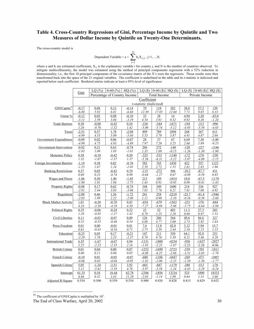
Table 4 reports results for ten separate and distinct multiple regressions. In column 1, the

dependent variable is the Gini coefficient. In the next three columns, the dependent variable

is the percentage of total income received by respectively; the poorest quintile, LQ(%), the

lowest 60% of the population, 0-60(%), and the richest quintile, HQ(%).

The right most six columns report regressions where average dollar income per capita is the

dependent variable. Again, there are separate regressions for the poorest quintile, LQ($), the

lowest 60% of the population, 0-60($), and the richest quintile, HQ($). In this case, however,

we consider two alternative estimates of quintile income per capita.

The first, labeled “Total Income” is the same as we have been using heretofore,

gij=(πijGiNi)/(Ni/5)=5πijGi where Gi is average income per capita (GNI/Capita) for country i,

Ni is the population, and πij is the percentage that quintile j consumes in country i. A possible

difficulty with this definition is its implicit assumption that government spending represents

income to each quintile in proportion to that quintile’s consumption. For some government

expenditures such as direct cash transfer payments, this is probably acceptable (since the

transfer payments are generally spent on consumption purchases.) However, for government


9

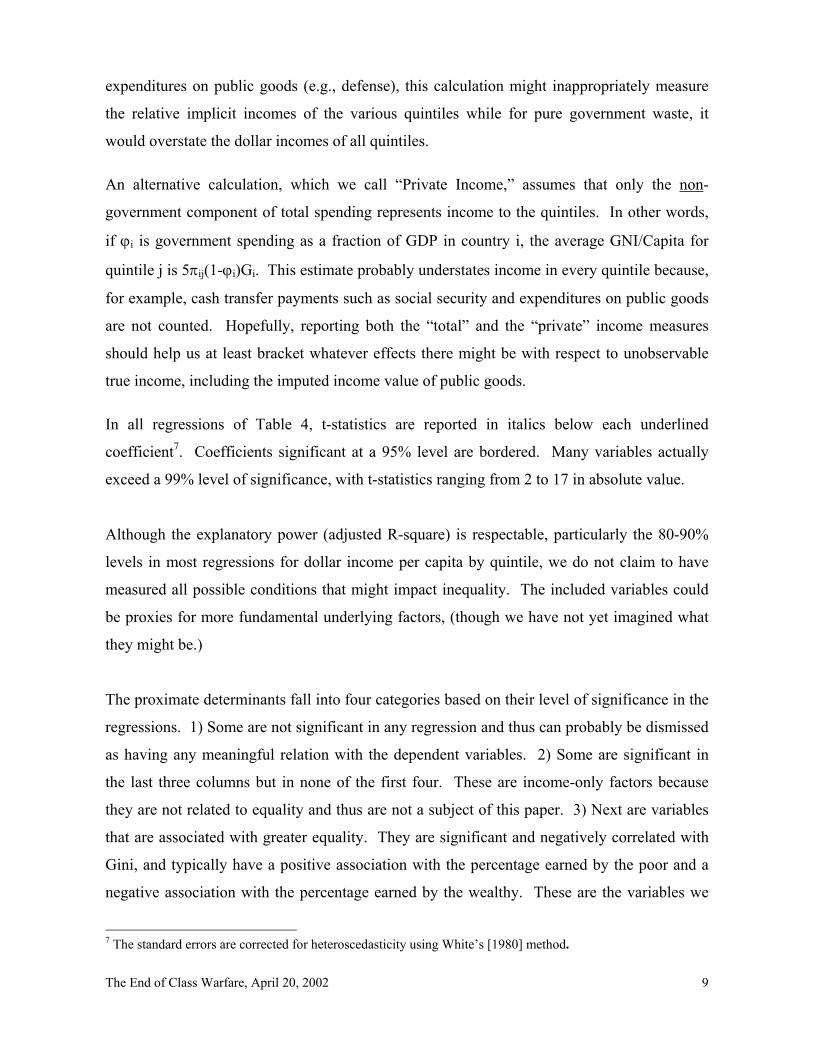
expenditures on public goods (e.g., defense), this calculation might inappropriately measure

the relative implicit incomes of the various quintiles while for pure government waste, it

would overstate the dollar incomes of all quintiles.

An alternative calculation, which we call “Private Income,” assumes that only the non-

government component of total spending represents income to the quintiles. In other words,

if ϕi is government spending as a fraction of GDP in country i, the average GNI/Capita for

quintile j is 5πij(1-ϕi)Gi. This estimate probably understates income in every quintile because,

for example, cash transfer payments such as social security and expenditures on public goods

are not counted. Hopefully, reporting both the “total” and the “private” income measures

should help us at least bracket whatever effects there might be with respect to unobservable

true income, including the imputed income value of public goods.

In all regressions of Table 4, t-statistics are reported in italics below each underlined

coefficient7. Coefficients significant at a 95% level are bordered. Many variables actually

exceed a 99% level of significance, with t-statistics ranging from 2 to 17 in absolute value.

Although the explanatory power (adjusted R-square) is respectable, particularly the 80-90%

levels in most regressions for dollar income per capita by quintile, we do not claim to have

measured all possible conditions that might impact inequality. The included variables could

be proxies for more fundamental underlying factors, (though we have not yet imagined what

they might be.)

The proximate determinants fall into four categories based on their level of significance in the

regressions. 1) Some are not significant in any regression and thus can probably be dismissed

as having any meaningful relation with the dependent variables. 2) Some are significant in

the last three columns but in none of the first four. These are income-only factors because

they are not related to equality and thus are not a subject of this paper. 3) Next are variables

that are associated with greater equality. They are significant and negatively correlated with

Gini, and typically have a positive association with the percentage earned by the poor and a

negative association with the percentage earned by the wealthy. These are the variables we

7 The standard errors are corrected for heteroscedasticity using White’s [1980] method.


10

are most interested in considering as possible correlates and we shall discuss them in detail

below. 4) Finally, some variables are associated with greater inequality. They have positive

coefficients in the Gini regression and positive (negative) coefficients in richest (poorest)

percentage regressions. Following is a summary categorization of these variables:

Insignificant

Government Intervention, Banking Restrictions, Wages and Prices.

Affects Average Income Only – No Inequality Significance

Trade Barriers(-), Monetary Policy (Inflation)(-), Foreign Investment

Barriers(+), Political Rights (+), Civil Liberties(+), Freedom of the Press(+),

British Colonization(-), French Colonization(-).

Greater Equality

GNI/Capita, Union %, Taxes, Government Expenditures, Property Rights,

Regulation, Education.

Greater Inequality

Black Market Activity, International Trade, Spanish Colonization.

Before discussing variables in the last two groups, we would be remiss by not saying a brief

word about some of the conditions that turn out to have no relation to equality. One can

readily concoct a story about each variable in the first two groups. The British and French

consulates should be pleased that their former colonies are relatively egalitarian, (though

significantly poorer than the average country in our study). The only real surprise is that none

of the democratic variables, and here we are talking about Political Rights, Civil Liberties and

Freedom of the Press, has any significant association with equality.

In another paper (Roll and Talbott [2001]) we find that these three democratic factors are all

highly positively significant in explaining country income and growth; and we see in Table 4

that high income is one of the most significant correlates of more equality. This seems to

imply that democracy has a positive impact on equality, but mainly because it is associated

with higher average income. Once average income is taken into account, democracy itself

seems to exert no further egalitarian influence.


11

GNI/Capita

Based on the magnitude of its t-statistics in every regression, average GNI/capita is the most

significant of all our variables. Higher average income is strongly associated with higher

incomes in all quintiles from poor to rich. Note that this result is not an a priori tautology

since the percentage earned by a given quintile could have, in principle, been adversely

impacted by higher average income for the entire country. Of course, if the percentages were

not affected by average income, there would necessarily be a positive algebraic relation

between the income in each quintile and the average.

But this is not, in fact, the situation. Notice that the Gini coefficient declines with

GNI/Capita, thereby revealing more equality in richer countries. Also, as shown in

regressions 2 through 4, the percentages earned by the poorest quintile and by the lowest three

quintiles are positively related to average income, while the percentage earned by the richest

quintile (regression 5) is negatively related to the average. In other words, greater equality

with higher average income implies a negative relative impact on the rich, but it is of

insufficient magnitude to make the rich worse off in an absolute sense.

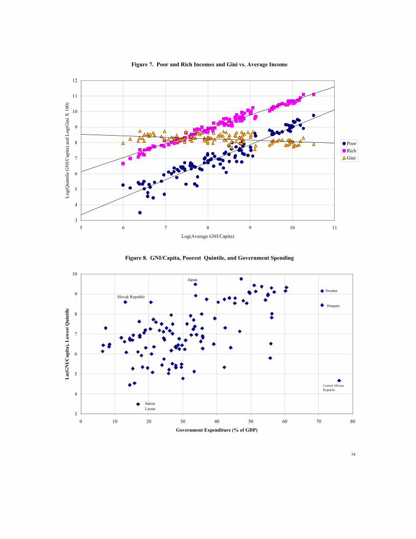
These effects are depicted in Figure 7, which plots poorest and richest quintile incomes and

Gini against average GNI/Capita for our expanded sample of 113 countries.8 The (bivariate)

line of best fit is also plotted. The slope of the line through the poorest incomes is 1.13 (t-

statistic 30.9) while the slope through the richest is somewhat lower, 0.929 (t-statistic 69.6).

Their difference is highly statistically significant.9 The slope of the Gini line is –0.103 (t-

statistic 5.15.) Hence, the negative inequality/income relation is weaker than either of the

positive quintile/average income relations, but it is still very significant. In conclusion, higher

average income is very strongly associated with higher incomes for both rich and poor, with

the association being somewhat more pronounced for the poor.

Some researchers argue that inequality is the cause of slow development rather than the effect

(Alesina and Rodrik [1994]), (Persson and Tabellini [1994], Clarke [1995]). They suggest that

as inequality increases there is no immediate effect on income, but the poor and middle

8 The natural logarithms of all variables are used to make the plot more linear. 9 This is based on a regression of the difference between poorest and richest GNI/Capita against the country average GNI/Capita (not reported); the slope coefficient has a t-statistic of 4.07.


12

classes eventually rise up as a new majority and force through policies damaging to growth.

This argument implies that minimum wage laws, government programs for the poor, union

formation and other actions the poor might take to address inequality could be bad for growth.

At least in the case of union participation and higher government spending, we find little

supporting evidence; both are associated with higher dollar Total incomes for all classes

(columns 5-7 of Table 4) although the association between union participation and rich Total

income is insignificant. The coefficients are negative for the rich when the narrower

definition, Private income, is employed, (regression 10), but they are not significant.

Moreover, Forbes [2000] disputes previous research and argues that currently high levels of

inequality are associated with more rapid growth, not less growth, in subsequent periods.

Forbes argues that previous contrary findings are attributable to a combination of poor quality

data and omitted variables. By using panel estimation, (dummy variables for individual

countries and time periods), and only “high quality” data, she claims to have partially

overcome these difficulties. Country dummies in the panel estimation control for omitted

variables across countries, but imperfectly unless they remain constant over time in each

country. Some possible omitted variables she mentions explicitly, (p. 885), as possible

culprits include corruption and education, which are two of the 21 proximate determinants we

employ in this paper; (black market activity is our proxy for corruption.)

If Forbes is right that inequality will lead to higher future growth, how does it happen that

richer countries currently have more equal distributions of income? Rich countries had more

rapid growth in the past, so to reconcile Forbes’ result with current conditions, these countries

must have had higher initial inequality, before their growth spurts, followed by a reversal to

more equality after they became rich. Though possible, this is a convoluted tale compared to

the simple story that growth is the engine behind greater equality.

We suspect that Forbes’ results are sensitive to her sample of countries (employed because of

their high quality data.) There are 45 countries in all, mostly large and none from sub-Sahara

Africa. (See her Table 2, p. 875.) For almost all the included countries, there is minimal

intertemporal variation in Gini coefficients, Forbes’ inequality measure, which suggests that


13

the observed level of statistical significance could depend on only a handful of countries,

those that have gone through at least moderate alterations in equality.

Using similar country data, we verified that the Gini coefficient is positively related to next

period’s growth and is statistically significant, a t-statistic of 2.18. But after removing just

two countries, Finland and Trinidad and Tobago, the t-statistic drops to 1.13. These two

countries were intentionally selected for removal because they had meaningful changes in

Gini over time, so we cannot claim that Forbes’ results are insignificant. Nonetheless, since

much of the information in the Forbes sample appears to reside in two relatively small

countries, one is entitled to wonder about the generality of her conclusion.

Property Rights, Black Market Activity and Regulation

Table 4 shows that strong property rights are negatively (and significantly) associated with the

Gini coefficient. The association between strong property rights and equality is also

supported by the income percentage regressions, a positive effect for the poor and a negative

effect for the rich. Yet strong property rights are positively related to dollar income levels of

all classes from rich to poor, regardless of the definition of income. If truly causative, it is a

second example (after average country income per capita) of a condition that benefits

everybody positively (de Soto [2000]), and also contributes to reduced inequality.

The connection between property rights and wealth is complex. Consider that individuals

without property have little incentive to fight for strong property rights laws, so very poor

countries would not likely have many citizens who care about them. Distributing property

more broadly by enacting land reform, formalizing rights to squatters’ de facto possessions, or

arranging some kind of ESOP where workers accumulate an ownership position, might lead

to more popular enthusiasm for strong property rights. Programs that encourage ownership,

such home mortgage interest deductibility, might indirectly promote popular support for

strong property rights legislation. Perhaps this would feed-forward and bring improvement in

both equality and average income.

Land reform need not entail confiscation. There are large swaths of unoccupied public land in

some countries that, by being distributed, could bring the pride of ownership to the current


14

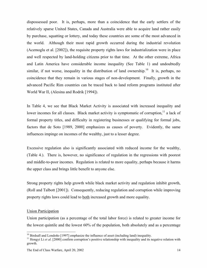
dispossessed poor. It is, perhaps, more than a coincidence that the early settlers of the

relatively sparse United States, Canada and Australia were able to acquire land rather easily

by purchase, squatting or lottery, and today these countries are some of the most advanced in

the world. Although their most rapid growth occurred during the industrial revolution

(Acemoglu et al. [2002]), the requisite property rights laws for industrialization were in place

and well respected by land-holding citizens prior to that time. At the other extreme, Africa

and Latin America have considerable income inequality (See Table 1) and undoubtedly

similar, if not worse, inequality in the distribution of land ownership.10 It is, perhaps, no

coincidence that they remain in various stages of non-development. Finally, growth in the

advanced Pacific Rim countries can be traced back to land reform programs instituted after

World War II, (Alesina and Rodrik [1994]).

In Table 4, we see that Black Market Activity is associated with increased inequality and

lower incomes for all classes. Black market activity is symptomatic of corruption,11 a lack of

formal property titles, and difficulty in registering businesses or qualifying for formal jobs,

factors that de Soto [1989, 2000] emphasizes as causes of poverty. Evidently, the same

influences impinge on incomes of the wealthy, just to a lesser degree.

Excessive regulation also is significantly associated with reduced income for the wealthy,

(Table 4.). There is, however, no significance of regulation in the regressions with poorest

and middle-to-poor incomes. Regulation is related to more equality, perhaps because it harms

the upper class and brings little benefit to anyone else.

Strong property rights help growth while black market activity and regulation inhibit growth,

(Roll and Talbott [2001]). Consequently, reducing regulation and corruption while improving

property rights laws could lead to both increased growth and more equality.

Union Participation

Union participation (as a percentage of the total labor force) is related to greater income for

the lowest quintile and the lowest 60% of the population, both absolutely and as a percentage 10 Birdsall and Londoño [1997] emphasize the influence of asset (including land) inequality. 11 Hongyi Li et al. [2000] confirm corruption’s positive relationship with inequality and its negative relation with growth.


15

of total country income. However, the dollar income coefficients are statistically significant

only for the broad definition, Total income. The wealthy share of country income falls with

greater unionization, but there is no significant association with the absolute income level of

the wealthy.12

One might expect to find unionization increasing as countries develop from a heavy

dependence on agriculture into more manufacturing. We attempted to control for this effect

by including average GNI/capita in the regression as an independent variable, but one can

never be sure that such a maneuver is adequate. Principal Components (PC) regression was

effective in eliminating other variables that seemed to have no explanatory relationship with

inequality but were highly correlated with income; e.g., trade barriers, inflation and the

democracy-related variables. So we put some credence on the possibility that unionization

has its own separate influence. We find no evidence that unions impede development.

Richard Freeman [1993] argues that unions, minimum wage laws, food subsidies and

employment protection laws - typically labeled as anti-growth - did little in the 1980’s to

prevent growth in the developed world. Also, they did not retard structural adjustment

programs and the concomitant reductions in wages in the developing world.

Taxes and Government Expenditures

Taxes and Government Expenditures (as a percentage of GDP) are associated with higher

incomes per capita;13 the strength of the relation is higher for the poor. This is reflected in the

inequality measures. Gini declines with government expenditures and the fraction earned by

the rich (poor) declines (increases.) The positive association between government spending

and both the relative and absolute incomes of the poor seems to make intuitive sense. After

all, many government programs are intended to benefit this group. Figure 8 presents a simple

bivariate plot of the (log) GNI/Capita for the poorest quintile against government spending for

the expanded sample of 113 countries. There is indeed a strongly positive correlation.14

12 The sign of the coefficient is positive (14) using Total income and negative (-45) using Private income, but neither is significant. 13 Except for government spending and the richest quintile using the Private measure of income. In this case, the coefficient is negative but insignificant. 14 A few of the more prominent outliers are tagged in the figure. Some of these, such as the Central African Republic, might very well represent suspicious data.


16

The positive relation between taxes and the richest incomes might seem counter-intuitive.

Perhaps taxes are proxying for some other positive government attribute. For instance, La

Porta et al. [1998] in their study “The Quality of Government” found “that the better

performing governments are also larger, and collect higher taxes”. The rich could benefit also

from a well-functioning government that promotes societal stability by providing some care

for the poor; Cf. Olson [1986]. Friedman [1962] suggests that a negative income tax would

be an efficient mechanism for achieving this desirable result.

Education

Education is related to higher absolute incomes for all classes and also to greater equality.15

Edwards [1997] finds that “countries that improved their education system…, experienced a

reduction in inequality.” This makes sense because education here is measured by the

average number of years of schooling completed by age 25. Because there is a limit to how

much schooling a wealthy student can acquire, the poor might benefit from education more

than proportionately. Education is clearly one possible avenue for the poor to climb out of

their unfavorable position. Education, however, is not free. It is a real investment that

implies foregoing other possible investments along the avenue to development. If the effect

really is causative, there is good news in that education brings greater prosperity and a more

egalitarian society.

Of course, the causality could actually be reversed. An elite class, in an attempt to defend its

privileged and very unequal position, might close off opportunities for the poor to advance

themselves through education. There could also be a gender issue. On average, women in

unequal poor countries are not encouraged to remain in school as long as men. In some cases,

such as in Taliban-controlled Afghanistan, women were blatantly excluded.

15 The coefficient is only marginally significant in the regression for the percentage earned by the poorest quintile.


17

International Trade

The level of International Trade is related to exacerbated inequality, a higher Gini and a larger

gap between the rich and poor, along with lower absolute incomes of the poorest and lowest

three quintiles. The relation of trade levels to absolute income is marginal and insignificant

for the rich. One interpretation is that trade per se has only a moderate net influence on the

total income of a country, but that it does have some distributional effect, perhaps owing to

relatively greater international competitive wage pressure on the poor.

Again, however, one must be cautious about the direction of causation. An alternative

interpretation is that more unequal countries engage in more trade because their richer citizens

have no access to locally produced manufactured luxuries. (There aren’t any.) They pay for

such imports by exporting cheap goods, (such as cloth, bananas, and beef), produced with

inexpensive labor.

Trade Barriers are unrelated to inequality. This result supports Edwards [1997], who argued

that opening trade does not exacerbate inequality for developing countries. Supporters of free

trade argue now that openness, rather than trade level, is the most important influence on

factor price equalization. Similarly, technological advancement comes with openness and

serves to reduce the distorting effects of local monopolies. Openness (an absence of barriers)

is associated with higher average income, (Roll and Talbott [2001]), so it could still have an

indirect positive influence on equality.

Why are more developing countries not promoting trade openness? The answer could very

well reside in the observation that trade barriers are useful in maintaining a system of official

corruption. Competition from the exterior would reduce the gains from bribery, lower the

private benefits from granting special import licenses and lower the payoffs from winking at

smugglers. Trade barriers are correlated with black market activity, another possible

corruption indicator; see Table 3. There may also be temporary hardships on the citizenry as

it shifts from an agrarian to an industrial society that may dampen its enthusiasm for openness

to new technology.


18

Spanish Colonization

Previous Spanish colonies have greater inequality, ceteris paribus, and absolute incomes of

their poor are significantly lower. As this is an exogenous variable the causality direction is

fairly certain, though the observed effect could be a proxy for something else. For instance,

Catholicism is the dominant religion in most former Spanish colonies and some believe that

religion has been cynically manipulated by the upper class to keep the poor in line. In some

countries of Latin America and the Caribbean, this allegedly has an ethnic component; i.e.,

descendents of European immigrants make up much of the upper class while native people

and African immigrants are the faithful (and the poor.)

VI. Conclusion. Wealthier countries are more egalitarian. After controlling for average income (the single

variable with the strongest egalitarian association), we find other conditions also that are

positively associated with greater equality. Property rights, unions, taxes, and government

spending all share the same feature: they are negatively and significantly related to the Gini

coefficient (a composite measure of inequality) and to the fraction of income earned by the

richest quintile, while they are positively and significantly associated with the fractions

earned by the poorest quintile and by the poorest 60% of the population. Other conditions

such as regulation and education are also related to more equality, but are less pervasively

significant.

Somewhat surprisingly, although the wealthiest earn relatively less under these conditions,

their absolute dollar incomes are either significantly higher or else insignificant in all cases

except under excessive regulation. This suggests that poor countries can become richer in

general and more egalitarian without any class losing ground in an absolute sense.

Some conditions are associated with greater inequality and with lower incomes for all classes.

These include black market activity, the level of international trade, and being a former

Spanish colony. Trade barriers and democracy-related conditions such as freedom of the

press, civil liberties, and political rights are all related to higher absolute incomes but appear

to have no association with inequality.


19

By focusing attention on average income per capita by class rather than on percentages earned

by class, much of the incitement for class confrontation appears to evaporate. The rich and

the poor have more congruent interests than they appear to realize and certainly more than

either side admits.


20

References Acemoglu, Daron, Simon Johnson, and James A. Robinson. 2002. “Reversal of Fortune: Geography and Instituitions in the Making of the Modern World Income Distribution.” Quarterly Journal of Economics, (forthcoming). Currently available at the following web site: http://econ-www.mit.edu/faculty/acemoglu/files/papers/qjerffinal1.pdf. (March). Alesina, Alberto, and Roberto Perotti. 1996. “Income Distribution, Political Instability, and Investment.” European Economic Review 40, 6 (June), 1203 –28. Alesina, Alberto, and Dani Rodrik. 1994. “Distributive Politics and Economic Growth.” Quarterly Journal of Economics 109 (May), 465 –90. Birdsall, Nancy, and Juan Luis Londoño. 1997. “Asset Inequality Matters: An Assessment of the World Bank’s Approach to Poverty Reduction.”American Economic Review 87, 2 (May), 32-37. Central Intelligence Agency. 2001. CIA World Factbook. Washington, D. C.: Central Intelligence Agency; Supplier of Documents. Clarke, George, R. G., 1995, “More evidence on income distribution and growth,” Journal of Development Economics 47, 2 (August), 403-427. De Soto, Hernando. 1989. The Other Path: The Invisible Revolution in the Third World. New York: Harper and Row. __________. 2000. The Mystery of Capital. Why Capitalism Triumphs in the West and Fails Everywhere Else. New York: Basic Books -Perseus Books Group. Edwards, Sebastian. 1997. “Trade Policy, Growth, and Income Distribution.” American Economic Review 87, 2 (May), 205-210. Forbes, Kristin J., 2000, “A Reassessment of the Relationship Between Inequality and Growth,” American Economic Review 90, 4 (September), 869-887. Freeman, Richard B. 1993. “Labor Markets and Institutions in Economic Development.” American Economic Review 83, 2 (May), 403-408. Friedman, Milton. 1962. Capitalism and Freedom. Chicago, IL: University of Chicago Press. Jha, Sailesh K. 1996. The Kuznets Curve: A Reassessment.” World Development 24, 4, 773-780. Judge, George C., W. E. Griffiths, R. Carter Hill, Helmut Lütkepohl, and Tsoung-Chao Lee, 1985, The Theory and Practice of Econometrics, (New York: Wiley.) Kuznets, Simon. 1955. “Economic Growth and Income Inequality.” American Economic Review 45,1 (March), 1-28.


21

La Porta, Rafael, Florencio Lopez-de-Silanes, Andrei Shleifer, and Robert Vishny. 1998. “The Quality of Government.” Journal of Law, Economics and Organization 15, 222-279. Li, Hongyi, Lixin Colin Xu, and Heng-Fu Zou. 2000. “Corruption, Income Distribution, and Growth.” Economics and Politics 12, 2 (July), 155-182. Olson, Mancur, 1986, Why Some Welfare-State Redistribution to the Poor Is a Great Idea, in Charles K. Rowley, ed., Public Choice and Liberty: Essays in Honor of Gordon Tullock, (Oxford: Basil Blackwell.) Persson, Torsten, and Guido Tabellini. 1994. “Is Inequality Harmful for Growth? Theory and Evidence.” American Economic Review 84, 3 (June), 600 –21. Roll, Richard, and John Talbott. 2001. “Why Many Developing Countries Just Aren’t.” Working paper. On http://www.anderson.ucla.edu/acad_unit/finance/wp/2001/19-01.pdf. (November). Thorton, John. 2001. “The Kuznets Inverted-U Hypothesis: Panel Data Evidence from 96 Countries.” Applied Economics Letters 8, 15-16. White, H., 1980. “A Heteroskedasticity-Consistent Covariance Matrix Estimator and a Direct Test for Heteroskedasticity”, Econometrica 48, 817-838.


22

Appendix

The Gini Coefficient

The Gini coefficient, named for the Italian statistician Corrado Gini, (1994-1964), is based on the area under the “Lorenz curve.” The Lorenz curve plots cumulative income as a fraction of total country income on the y-axis, from poorest to richest, against the cumulative fraction of the population on the x-axis. By construction, the resulting curve passes through the origin and also through the point (1,1) corresponding to 100% of the population and 100% of the income. If everyone had exactly the same income, the Lorenz curve would be a 45º line, but actual populations are unequal so the curve usually appears something like Figure A-1. The lightly shaded area under the curve is smaller the greater the inequality of incomes across the population. Call the lightly shaded area L and note that 0 ≤ L ≤½. The Gini coefficient is 1-2L, so it varies between zero, complete equality and 1.0, complete inequality. The darker shaded area is one-half Gini. Although the merits of the Gini coefficient could be and have been disputed, it remains one of the most popular composite measures of income inequality.

Figure A-1

0

0.1

0.2

0.3

0.4

0.5

0.6

0.7

0.8

0.9

1

0 0.1 0.2 0.3 0.4 0.5 0.6 0.7 0.8 0.9 1

Fraction of Population

Frac

tion

of In

com

e

L

Lorenz Curve

Gini/2


23

Table 1. Gini Coefficients, Percentages Earned by Quintile, and Total Income per Capita (from the 1990s)16

Poor 2 3 4 Rich

Country Gini (%) Percentage of Income by Quintile17

Income/ Capita ($)

Algeria * 35.3 7.0 11.6 16.1 22.7 42.6 4,560 Armenia 44.4 5.5 9.4 13.9 20.6 50.6 2,019 Australia * 35.2 5.9 12.0 17.2 23.6 41.3 21,030

Austria * 23.1 10.4 14.8 18.5 22.9 33.3 22,577 Azerbaijan 36.0 6.9 11.5 16.1 22.3 43.3 1,962

Bangladesh * 33.6 8.7 12.0 15.7 20.8 42.8 1,344 Belarus 21.7 11.4 15.2 18.2 21.9 33.3 5,286

Belgium * 25.0 9.5 14.6 18.4 23.0 34.5 23,092 Bolivia * 58.9 1.9 5.9 11.1 19.3 61.8 2,189

Brazil * 59.1 2.6 5.7 10.3 18.5 63.0 6,647 Bulgaria 26.4 10.1 13.9 17.4 21.9 36.8 4,912

Burkina Faso 48.2 5.5 8.7 12.0 18.7 55.0 844 Burundi 33.3 7.9 12.1 16.3 22.1 41.6 574

Cambodia 40.4 6.9 10.7 14.7 20.1 47.6 1,337 Canada * 31.5 7.5 12.9 17.2 23.0 39.3 22,499

Central African Republic 61.3 2.0 4.9 9.6 18.5 65.0 1,066 Chile * 57.5 3.4 6.3 10.5 17.9 62.0 7,726 China * 40.3 5.9 10.2 15.1 22.2 46.6 2,758

Colombia * 57.1 3.0 6.6 11.1 18.4 60.9 5,886 Costa Rica * 45.9 4.5 8.9 14.1 21.6 51.0 5,737

Croatia 29.0 8.8 13.3 17.4 22.6 38.0 6,420 Czech Republic 25.4 10.3 14.5 17.7 21.7 35.9 12,871

Denmark * 24.7 9.6 14.9 18.3 22.7 34.5 23,407 Dominican Republic * 47.4 5.1 8.6 13.0 20.0 53.3 4,017

Ecuador * 43.7 5.4 9.4 14.2 21.3 49.7 3,001 Egypt * 28.9 9.8 13.2 16.6 21.4 39.0 2,976

El Salvador * 50.8 3.7 7.8 12.8 20.4 55.3 4,018 Estonia 37.6 7.0 11.0 15.3 21.6 45.1 6,811

Ethiopia 40.0 7.1 10.9 14.5 19.8 47.7 591 Finland * 25.6 10.0 14.2 17.6 22.3 35.8 18,885 France * 32.7 7.2 12.6 17.2 22.8 40.2 20,813

Gambia * 47.8 4.4 9.0 13.5 20.4 52.8 1,428 Georgia 37.1 6.1 11.4 16.3 22.7 43.6 2,982

Germany * 30.0 8.2 13.2 17.5 22.7 38.5 21,713 Ghana * 39.6 5.9 10.4 15.3 22.5 45.9 1,730

16 Countries with asterisks constitute the sample for the multivariate analysis. 17 Since the percentages are based on consumption surveys or similar sources, they are effectively after tax. They should include direct government transfers. Average country income (or GNI) is pre-tax.


24

Greece * 32.7 7.5 12.4 16.9 22.8 40.3 13,620 Guatemala * 55.8 3.8 6.8 10.9 17.9 60.6 3,431

Guinea 40.3 6.4 10.4 14.8 21.2 47.2 1,723 Guinea Bissau 56.2 2.1 6.5 12.0 20.6 58.9 817

Guyana 40.2 6.3 10.7 15.0 21.2 46.9 3,153 Honduras * 59.0 1.6 5.6 11.0 20.1 61.8 2,313 Hungary * 24.4 10.0 14.7 18.3 22.7 34.4 9,252

India * 37.8 8.1 11.6 15.0 19.3 46.1 1,979 Indonesia * 31.7 9.0 12.5 16.1 21.3 41.1 2,963

Ireland * 35.9 6.7 11.6 16.4 22.4 42.9 16,079 Israel * 35.5 6.9 11.4 16.3 22.9 42.5 17,366 Italy * 27.3 8.7 14.0 18.1 22.9 36.3 20,485

Ivory Coast 36.7 7.1 11.2 15.6 21.9 44.3 1,622 Jamaica * 36.4 7.0 11.5 15.8 21.8 43.9 3,509

Japan * 24.9 10.6 14.2 17.6 22.0 35.7 24,804 Jordan * 36.4 7.6 11.4 15.5 21.1 44.4 2,752

Kazakstan 35.4 6.7 11.5 16.4 23.1 42.3 4,404 Kenya * 44.5 5.0 9.7 14.2 20.9 50.2 993

Korea, South * 31.6 7.5 12.9 17.4 22.9 39.3 14,305 Kyrgyz Republic 40.5 6.3 10.2 14.7 21.4 47.4 2,108

Laos 37.0 7.6 11.4 15.3 20.8 45.0 1,649 Latvia 32.4 7.6 12.9 17.1 22.1 40.3 5,218

Lesotho 56.0 2.8 6.5 11.2 19.4 60.1 2,343 Lithuania 32.4 7.8 12.6 16.8 22.4 40.3 5,815

Luxembourg 26.9 9.4 13.8 17.7 22.6 36.5 36,509 Madagascar 46.0 5.4 9.2 13.4 19.9 52.0 742

Malaysia * 49.2 4.4 8.1 12.9 20.3 54.3 8,260 Mali * 50.5 4.6 8.0 11.9 19.3 56.2 663

Mauritania 37.3 6.4 11.2 16.0 22.4 44.1 1,499 Mexico * 51.9 4.0 7.6 12.2 19.6 56.7 7,055

Moldova 40.6 5.6 10.2 15.2 22.2 46.8 2,222 Mongolia 33.2 7.3 12.2 16.6 23.0 40.9 1,454 Morocco 39.2 6.5 10.6 14.8 21.3 46.6 3,247

Mozambique 39.6 6.5 10.8 15.1 21.1 46.5 637 Nepal * 36.7 7.6 11.5 15.1 21.0 44.8 1,183

Netherlands * 32.6 7.3 12.7 17.2 22.8 40.1 21,740 Nicaragua * 60.3 2.3 5.9 10.4 17.9 63.6 1,780

Niger 50.5 2.6 7.1 13.9 23.1 53.3 720 Nigeria 50.6 4.4 8.2 12.5 19.3 55.7 762 Norway * 25.8 9.7 14.3 17.9 22.2 35.8 25,844 Pakistan * 31.2 9.5 12.9 16.0 20.5 41.1 1,724 Panama * 48.5 3.6 8.1 13.6 21.9 52.8 4,959


25

Papua New Guinea * 50.9 4.5 7.9 11.9 19.2 56.5 2,466 Paraguay * 57.7 1.9 6.0 11.4 20.1 60.7 4,609

Peru * 46.2 4.4 9.1 14.1 21.3 51.2 4,260 Philippines * 46.2 5.4 8.8 13.2 20.3 52.3 3,819

Poland * 31.6 7.8 12.8 17.1 22.6 39.7 7,000 Portugal * 35.6 7.3 11.6 15.9 21.8 43.4 14,026 Romania 28.6 8.9 13.6 17.6 22.6 37.3 6,698

Russia 48.7 4.4 8.6 13.3 20.1 53.7 6,780 Rwanda * 28.9 9.7 13.2 16.5 21.6 39.1 400 Senegal * 41.3 6.4 10.3 14.5 20.6 48.2 1,262

Sierra Leone 62.9 1.1 2.0 9.8 23.7 63.4 597 Slovak Republic 19.5 11.9 15.8 18.8 22.2 31.4 9,083

Slovenia 28.4 9.1 13.4 17.3 22.5 37.7 13,640 South Africa * 59.3 2.9 5.5 9.2 17.7 64.8 8,645

Spain * 32.5 7.5 12.6 17.0 22.6 40.3 15,437 Sri Lanka * 34.4 8.0 11.8 15.8 21.5 42.8 2,793 Swaziland 60.9 2.7 5.8 10.0 17.1 64.4 4,327

Sweden * 25.0 9.6 14.5 18.1 23.2 34.5 19,519 Switzerland * 33.1 6.9 12.7 17.3 22.9 40.3 26,677

Tanzania 38.2 6.8 11.0 15.1 21.6 45.5 474 Thailand * 41.4 6.4 9.8 14.2 21.2 48.4 6,378

Trinidad and Tobago * 40.3 5.5 10.3 15.5 22.7 45.9 6,571 Tunisia * 41.7 5.7 9.9 14.7 21.8 47.9 4,905 Turkey * 41.5 5.8 10.2 14.8 21.6 47.7 6,238

Turkmenistan 40.8 6.1 10.2 14.7 21.5 47.5 2,985 Uganda * 37.4 7.1 11.1 15.4 21.5 44.9 1,053 Ukraine 29.0 8.8 13.3 17.4 22.7 37.8 3,362

United Kingdom * 36.1 6.6 11.5 16.3 22.7 43.0 20,004 United States * 40.8 5.2 10.5 15.6 22.4 46.4 28,649

Uruguay * 42.3 5.4 10.0 14.8 21.5 48.3 8,209 Uzbekistan 33.3 7.4 12.0 16.7 23.0 40.9 2,042 Venezuela * 48.8 4.1 8.3 13.2 20.7 53.7 5,666

Vietnam 36.1 8.0 11.4 15.2 20.9 44.5 1,571 Yemen 33.4 7.4 12.2 16.7 22.5 41.2 657 Zambia * 52.6 3.3 7.6 12.5 20.0 56.6 721

Zimbabwe * 56.8 4.0 6.3 10.0 17.4 62.3 2,593

Mean 39.7 6.4 10.6 15.0 21.3 46.7 7,199 Minimum 19.5 1.1 2.0 9.2 17.1 31.4 400 Maximum 62.9 11.9 15.8 18.8 23.7 65.0 36,509


26

Table 1, Part 2 Some Important Countries Without Available Income Distribution Data

Albania Congo, Dem. Rep. of Iraq Puerto Rico Angola Congo, Republic of Korea, North Qatar Argentina Cuba Kuwait Samoa Bahamas Cyprus Lebanon Saudi Arabia Bahrain Djibouti Libya Singapore Barbados Equatorial Guinea Macedonia Somalia Belize Eritrea Malawi Sudan Benin Fiji Malta Suriname Bosnia Gabon Mauritius Syria Botswana Haiti Myanmar Taiwan Cameroon Hong Kong Namibia Tajikistan Cape Verde Iceland New Zealand Togo Chad Iran Oman United Arab Emirates


27

Table 2. Components of Variables as Described in Original Sources.

Banking Restrictions • Government ownership of banks. • Restrictions on the ability of foreign banks

to open branches and subsidiaries. • Government influence over the allocation

of credit. • Government regulations. • Freedom to offer all types of financial

services, securities, and insurance policies. • Source: Heritage Foundation (a).

Black Market Activity • Smuggling. • Piracy of intellectual property in the black

market. • • Agricultural production supplied on the

black market. • Manufacturing supplied on the black

market. • Services supplied on the black market. • Transportation supplied on the black

market. • Labor supplied on the black market. • Source: Heritage Foundation (a).

Civil Liberties • Equality of opportunity. • Rule of law, with people treated fairly

under the law, without fear of unjust imprisonment or torture.

• Freedom of press, association, religion, assembly, demonstration, discussion and organization.

• Source: Freedom House (b).

Colonization History • Dummy variable equal to one or zero with

one signifying prior colonization. • French, British and Spanish colonies

observed. • Source: Previous study on growth.

Education • Average number of years of schooling

attained by 25 year olds • Source: World Bank.

Foreign Investment Restrictions • Foreign investment code. • Restrictions on foreign ownership of

business. • Restrictions on the industries and

companies open to foreign investors.

• Restrictions and performance requirements on foreign companies.

• Foreign ownership of land. • Equal treatment under the law for both

foreign and domestic companies. • Restrictions on the repatriation of

earnings. • Availability of local financing for foreign

companies. • Source: Heritage Foundation (a).

Freedom of the Press • System of mass communication and its

ability to permit free flow of communication.

• Government laws and decisions that influence content of the media.

• Political or financial influence over the media.

• Oppression of the media. • Censure of the media. • Source: Freedom House (b).

Gini and Percentage Income by Quintiles • Based on surveys from 1991 to 1996. • Based on consumption or income. • GNI/capita • 1996 GNI per capita. • GNI adjusted for Purchasing Power Parity

(PPP). • Source: World Bank Data (PPP Adjusted)

and CIA World Factbook.

Government Expenditures • Government Expenditures as a % of total

GDP. • Government Expenditures include transfer

payments. • Source: Heritage Foundation (a).

Government Intervention in the Economy • Government consumption as a percentage

of the economy. • Government ownership of businesses and

industries. • Share of government revenues from state-

owned enterprises and government ownership of property.

• Economic output produced by the government.

• Source: Heritage Foundation (a).


28

International Trade • Level of trade as a % of GDP. • Source: World Bank.

Monetary Policy • Weighted average inflation rate from 1990

to 1999 with more recent data more heavily weighted.


Political Rights • Free elections. • Right to vote. • Self-determination. • Freedom from military and totalitarianism • Source: Freedom House (b).

Property Rights • Freedom from government influence over • the judicial system. • Commercial code defining contracts. • Sanctioning of foreign arbitration of

contract disputes. • Government expropriation of property. • Corruption within the judiciary. • Delays in receiving judicial decisions. • Legally granted and protected private

property. • Source: Heritage Foundation (a)(b).

Regulation • Licensing requirements to operate a

business. • Ease of obtaining a business license. • Corruption within the bureaucracy. • Labor regulations, such as established

work-weeks, paid vacations, and parental leave, as well as selected labor regulations.

• Environmental, consumer safety, and worker health regulations.

• Regulations that impose a burden on business.


Taxes • Top income tax rate. • Tax rate that the average taxpayer faces. • Top corporate tax rate. • Source: Heritage Foundation (a).

Trade Barriers • Average tariff rate. • Non-tariff barriers. • Corruption in the customs service. • Source: Heritage Foundation (a).

Union Participation • Union membership as a % of total labor

force. • Includes farming in labor force • Source: International Labour Organization.

Wages and Prices • Minimum wage laws. • Freedom to set prices privately without

government influence. • Government price controls. • The extent to which government price

controls are used. • Government subsidies to businesses that

affect prices. • Source: Heritage Foundation (a).

For ease of interpretation, we reversed the scale of four variables, Property Rights, Political Rights, Civil Liberties and Freedom of the Press, from their original source, so that now a larger value is associated intuitively with a higher degree of rights, liberty, and freedom. We also broke the Heritage Foundation’s Fiscal Burden Index into its two constituents, Taxes and Government Expenditures, in order to check their separate influences. Heritage’s Fiscal Burden index is the simple average of two of its own sub-indices, the first measuring levels of personal and corporate tax rates, and the second reflecting levels of government expenditures as a percentage of GDP. Heritage’s summary tax rating is our Taxes variable, and their raw government expenditures as a percentage of GDP is our Government Expenditures variable. We selected raw percentages for the Government Expenditures variable, because Heritage’s summary rating score is based on different scales for developed versus developing countries.

___________________________________________

(a) The 2001 Index of Economic Freedom. This Heritage publication provides a narrative description of each variable for every country. It is also available on the internet. The 2002 version is now available. (b) Original scale reversed, so that a larger value now means more.


29

Table 3. Correlations of Candidates for Determinants of Inequality.

GN

I/Cap

ita

Union % 0.546 Uni

on %

Trade Barriers -0.610 -0.221 Trad

e B

arrie

rs

Taxes 0.600 0.373 -0.298 Taxe

s

Government Expenditures 0.743 0.684 -0.404 0.565 Gov

ernm

ent E

xpen

ditu

res

Government Intervention 0.105 0.374 0.205 0.258 0.348 Gov

ernm

ent I

nter

vent

ion

Monetary Policy -0.705 -0.346 0.382 -0.466 -0.496 -0.099 Mon

etar

y Po

licy

Foreign Investment Barriers -0.316 -0.239 0.463 -0.157 -0.321 0.061 0.134 Fore

ign

Inve

stm

ent B

arrie

rs

Banking Restrictions -0.418 -0.257 0.427 -0.193 -0.289 0.088 0.349 0.486 Ban

king

Res

trict

ions

Wages and Prices -0.372 -0.267 0.339 -0.137 -0.314 0.008 0.256 0.437 0.559 Wag

es a

nd P

rices

Property Rights 0.751 0.411 -0.563 0.516 0.556 -0.071 -0.624 -0.343 -0.445 -0.312 Prop

erty

Rig

hts

Regulation -0.604 -0.350 0.422 -0.360 -0.497 -0.003 0.487 0.373 0.395 0.501 -0.629 Reg

ulat

ion

Black Market Activity -0.790 -0.481 0.462 -0.489 -0.658 -0.083 0.615 0.225 0.445 0.447 -0.743 0.554 Bla

ck M

arke

t Act

ivity

Political Rights 0.640 0.340 -0.437 0.295 0.538 -0.090 -0.419 -0.416 -0.303 -0.352 0.566 -0.514 -0.496 Polit

ical

Rig

hts

Civil Liberties 0.738 0.411 -0.564 0.330 0.575 -0.109 -0.509 -0.502 -0.415 -0.432 0.653 -0.514 -0.571 0.878 Civ

il Li

berti

es

Press Freedom 0.708 0.339 -0.520 0.334 0.585 0.013 -0.523 -0.403 -0.349 -0.381 0.656 -0.487 -0.580 0.879 0.892 Pres

s Fre

edom

Education 0.833 0.566 -0.521 0.412 0.641 0.026 -0.559 -0.409 -0.472 -0.455 0.698 -0.606 -0.678 0.610 0.698 0.634 Educ

atio

n

International Trade 0.118 0.181 0.033 -0.015 0.208 -0.010 -0.315 -0.038 -0.196 -0.075 0.274 -0.303 -0.194 0.088 0.137 0.142 0.209 Inte

rnat

iona

l Tra

de

British Colonization -0.148 -0.122 0.210 0.133 -0.045 0.075 -0.034 0.085 -0.007 0.015 0.035 -0.002 0.053 -0.158 -0.227 -0.131 -0.056 0.077 Brit

ish

Col

oniz

atio

n

French Colonization -0.206 0.038 0.288 -0.094 -0.118 0.083 0.106 0.088 0.075 0.114 -0.206 0.020 0.140 -0.233 -0.165 -0.198 -0.314 -0.020 -0.185 Fren

ch C

olon

izat

ion

Spanish Colonization -0.285 -0.261 -0.050 -0.508 -0.408 -0.283 0.364 -0.205 -0.072 -0.079 -0.315 0.175 0.343 -0.004 0.030 -0.085 -0.135 -0.101 -0.349 -0.147


30

Table 4. Cross-Country Regressions of Gini, Percentage Income by Quintile and Two

Measures of Dollar Income by Quintile on Twenty-One Determinants.

The cross-country model is

Dependent Variable = a + ∑=

21

1ij,iiXb , j=1,…,N,

where a and bi are estimated coefficients, Xi,j is the explanatory variable i for country j, and N is the number of countries observed. To mitigate multicollinearity, the model was estimated using the method of principal components regression with a 52% reduction in dimensionality; i.e., the first 10 principal components of the covariance matrix of the X’s were the regressors. Those results were then transformed back into the space of the 21 original variables. The coefficient is underlined in the table and its t-statistic is italicized and reported below each coefficient. Bordered entries indicate at least a 95% level of significance.

LQ (%) 0-60 (%) HQ (%) LQ ($) 0-60 ($) HQ ($) LQ ($) 0-60 ($) HQ ($)

Gini Percentage of Country Income Total Income Private Income

Coefficient t-statistic (italicized)

GNI/Capita18 -0.17 0.04 0.12 -0.14 79 118 282 38.8 57.3 130 -6.80 5.92 6.81 -6.68 12.39 17.05 12.68 7.71 9.85 8.33

Union % -0.12 0.03 0.08 -0.10 33 38 14 4.94 2.20 -45.0 -3.11 2.59 3.04 -3.19 4.54 3.91 0.32 0.92 0.26 -1.24

Trade Barriers 0.58 -0.08 -0.42 0.54 -336 -544 -1671 -194 -312 -996 1.26 -0.76 -1.32 1.42 -5.09 -5.74 -5.12 -4.95 -5.59 -4.65

Taxes -2.51 0.57 1.78 -2.04 499 789 1894 244 367 611 -4.99 4.53 5.09 -5.04 5.53 5.70 3.87 4.91 4.87 2.04

Government Expenditures -0.09 0.02 0.06 -0.07 28 37 67 6.69 7.58 -3.40 -4.99 4.75 4.93 -4.89 7.97 7.20 3.25 2.66 1.89 -0.23

Government Intervention -0.92 0.21 0.63 -0.74 206 272 -140 -128 -227 -1246 -1.03 1.09 1.05 -1.01 1.35 1.09 -0.15 -1.26 -1.30 -1.90

Monetary Policy 0.58 -0.10 -0.42 0.50 -325 -533 -1140 -172 -276 -530 1.32 -1.07 -1.37 1.37 -5.56 -6.31 -3.22 -5.07 -4.89 -2.15

Foreign Investment Barriers -1.19 0.38 0.82 -0.78 582 765 1430 422 557 1123 -1.25 1.67 1.24 -1.01 2.59 2.72 1.52 2.61 2.83 1.86

Banking Restrictions 0.57 0.05 -0.42 0.70 -115 -272 506 -10.2 -87.7 431 0.69 0.23 -0.74 0.99 -0.68 -1.27 0.67 -0.09 -0.59 0.85

Wages and Prices -1.86 0.50 1.40 -1.45 215 189 -1014 10.0 -67.5 -1170 -1.80 1.91 1.94 -1.75 1.43 0.91 -0.95 0.09 -0.41 -1.43

Property Rights -0.88 0.17 0.62 -0.74 344 549 1600 214 336 927 -2.91 2.44 3.03 -3.06 7.85 7.76 6.21 7.61 7.08 4.92

Regulation -2.08 0.46 1.56 -1.72 241 258 -2218 -23.7 -81.4 -1946 -2.03 1.89 2.22 -2.00 1.11 0.90 -2.10 -0.16 -0.39 -2.68

Black Market Activity 1.01 -0.20 -0.70 0.83 -454 -679 -1563 -253 -376 -844 4.24 -3.38 -4.19 4.30 -7.27 -8.69 -5.08 -5.75 -6.64 -3.98

Political Rights 0.35 -0.06 -0.24 0.32 23 52 403 11.3 27.3 203 1.29 -0.95 -1.27 1.42 0.79 1.25 2.20 0.69 0.97 1.52

Civil Liberties 0.11 -0.03 -0.07 0.09 126 206 564 49.6 86.6 227 0.52 -0.55 -0.46 0.54 4.09 4.77 3.00 2.73 2.92 1.63

Press Freedom 0.01 0.00 -0.01 0.01 7.6 13.8 42.0 3.12 5.94 15.7 0.61 -0.43 -0.54 0.71 2.75 3.59 2.44 2.10 2.15 1.15

Education -0.25 0.05 0.17 -0.21 147 211 550 64.1 92.8 253 -2.29 1.76 2.23 -2.37 8.78 8.76 5.38 6.21 5.46 3.28

International Trade 6.55 -1.67 -4.67 4.94 -1151 -1800 -4234 -958 -1437 -2927 2.25 -2.23 -2.35 2.16 -1.95 -2.25 -1.07 -2.23 -2.28 -0.96

British Colony 0.01 0.04 0.00 0.07 -1252 -1690 -3723 -539 -703 -1811 0.00 0.11 0.00 0.05 -6.09 -6.25 -2.86 -3.51 -3.05 -1.78

French Colony -0.10 0.01 -0.05 -0.07 -680 -1106 -4447 -269 -471 -2407 -0.06 0.03 -0.04 -0.05 -1.82 -2.06 -2.23 -1.50 -1.56 -1.77

Spanish Colony 5.05 -1.24 -3.51 3.92 -601 -847 -1179 -388 -513 -176 5.11 -5.62 -5.19 4.76 -3.97 -3.58 -1.24 -4.43 -3.29 -0.24

Intercept 61.35 0.54 16.44 62.78 -2386 -1856 13216 525 1890 18333 8.86 0.32 3.43 11.29 -2.03 -1.14 1.99 0.64 1.53 3.60

Adjusted R-Square 0.554 0.500 0.559 0.554 0.900 0.920 0.828 0.815 0.829 0.652

18 The coefficient of GNI/Capita is multiplied by 103.

31

Figure 1. Percentages of Income Earned by Poorest vs. Richest Quintile113 countries, 1990s

0

2

4

6

8

10

12

14

30.0 35.0 40.0 45.0 50.0 55.0 60.0 65.0 70.0

Richest Quintile Percentage

Poor

est Q

uint

ile P

erce

ntag

e

Figure 2. Log Income per Capita Earned by Poorest vs. Richest Quintile113 countries, 1990s

3

5

7

9

6 7 8 9 10 11 12

Log(GNI/Capita), Richest Quintile

Log

(GN

I/C

apita

), Po

ores

t Qui

ntile

32

Figure 3. Gini vs. GNI/Capita113 countries, 1990s

18

23

28

33

38

43

48

53

58

63

0 5,000 10,000 15,000 20,000 25,000 30,000 35,000 40,000

GNI/Capita

Gin

i

Figure 4. Gini vs. Log(GNI/Capita)113 countries, 1990s

18

23

28

33

38

43

48

53

58

63

5 6 7 8 9 10 11

Log(GNI/Capita)

Gin

i

33

Figure 5. Gini vs. Percentage Earned by Richest Quintile113 countries, 1990s

18

23

28

33

38

43

48

53

58

63

30.0 35.0 40.0 45.0 50.0 55.0 60.0 65.0

Percentage Earned by Richest Quintile

Gin

i

Figure 6. Gini vs. GNI/Capita of the Richest Quintile113 countries, 1990s

18

23

28

33

38

43

48

53

58

63

0 10000 20000 30000 40000 50000 60000 70000

GNI/Capita, Richest Quintile

Gin

i

34

Figure 7. Poor and Rich Incomes and Gini vs. Average Income

3

4

5

6

7

8

9

10

11

12

5 6 7 8 9 10 11

Log(Average GNI/Capita)

Log(

Qui

ntile

GN

I/Cap

ita) a

nd L

og(G

ini X

100

)

PoorRichGini

Figure 8. GNI/Capita, Poorest Quintile, and Government Spending

3

4

5

6

7

8

9

10

0 10 20 30 40 50 60 70 80

Government Expenditure (% of GDP)

Ln(

GN

I/C

apita

), L

owes

t Qui

ntile

Central AfricanRepublic

Sweden

Hungary

SierraLeone

Slovak Republic

Japan

Fifth Draft Dick - anderson.ucla.edu

Documents

Transcript of Fifth Draft Dick - anderson.ucla.edu