FIDELIO 1 - Europapublications.jrc.ec.europa.eu/repository/bitstream/JRC81864/lfna... · Contents...
149
Report EUR 25985 EN 2013 Kurt Kratena, Gerhard Streicher, Umed Temurshoev, Antonio F. Amores, Iñaki Arto, Ignazio Mongelli, Frederik Neuwahl, José M. Rueda-Cantuche, Valeria Andreoni FIDELIO 1: Fully Interregional Dynamic Econometric Long-term Input-Output Model for the EU27
Transcript of FIDELIO 1 - Europapublications.jrc.ec.europa.eu/repository/bitstream/JRC81864/lfna... · Contents...

Report EUR 25985 EN
2 0 1 3
Kurt Kratena, Gerhard Streicher, Umed Temurshoev,Antonio F. Amores, Iñaki Arto, Ignazio Mongelli, Frederik Neuwahl, José M. Rueda-Cantuche, Valeria Andreoni
FIDELIO 1: Fully Interregional Dynamic Econometric Long-term Input-Output Model for the EU27

European Commission
Joint Research Centre
Institute for Prospective Technological Studies
Contact information
Address: Edificio Expo. c/ Inca Garcilaso, 3. E-41092 Seville (Spain)
E-mail: [email protected]
Tel.: +34 954488318
Fax: +34 954488300
http://ipts.jrc.ec.europa.eu
http://www.jrc.ec.europa.eu
Legal Notice
Neither the European Commission nor any person acting on behalf of the Commission
is responsible for the use which might be made of this publication.
Europe Direct is a service to help you find answers to your questions about the European Union
Freephone number (*): 00 800 6 7 8 9 10 11
(*) Certain mobile telephone operators do not allow access to 00 800 numbers or these calls may be billed.
A great deal of additional information on the European Union is available on the Internet.
It can be accessed through the Europa server http://europa.eu/.
JRC81864
EUR 25985 EN
ISBN 978-92-79-30009-7 (pdf)
ISSN 1831-9424 (online)
doi:10.2791/17619
Luxembourg: Publications Office of the European Union, 2013
© European Union, 2013
Reproduction is authorised provided the source is acknowledged.
Printed in Spain
FIDELIO 1:Fully Interregional Dynamic Econometric
Long-term Input-Output Modelfor the EU27
Kurt Kratena, Gerhard Streicher, Umed Temurshoev,Antonio F. Amores, Inaki Arto, Ignazio Mongelli, Frederik Neuwahl,
Jose M. Rueda-Cantuche, Valeria Andreoni
May 22, 2013
Contents
Contents i
Preface vii
Glossary xi
1 Macro-overview of FIDELIO 1
2 Theoretical foundations of FIDELIO 15
2.1 Consumption block . . . . . . . . . . . . . . . . . . . . . . . . . . . . 15
2.1.1 Households’ demands for four types of durable and total non-durable commodities . . . . . . . . . . . . . . . . . . . . . . . 15
2.1.2 Splitting aggregate nondurable commodity into its differentcategories . . . . . . . . . . . . . . . . . . . . . . . . . . . . . 24
2.2 Production block . . . . . . . . . . . . . . . . . . . . . . . . . . . . . 29
2.2.1 The translog function . . . . . . . . . . . . . . . . . . . . . . . 30
2.2.2 Sectoral output prices and derived input demands . . . . . . . 31
2.3 Labour market . . . . . . . . . . . . . . . . . . . . . . . . . . . . . . 36
2.3.1 Demands for labour skill types . . . . . . . . . . . . . . . . . . 36
2.3.2 Wage curves . . . . . . . . . . . . . . . . . . . . . . . . . . . . 38
3 Derivation of the base-year data 43
3.1 Basic price data . . . . . . . . . . . . . . . . . . . . . . . . . . . . . . 43
3.2 Shares and structure matrices . . . . . . . . . . . . . . . . . . . . . . 44
i
ii CONTENTS
3.3 Trade matrix construction . . . . . . . . . . . . . . . . . . . . . . . . 50
3.4 COICOP-CPA bridge matrices . . . . . . . . . . . . . . . . . . . . . . 53
3.5 Consumption block residuals . . . . . . . . . . . . . . . . . . . . . . . 56
3.6 Production block residuals . . . . . . . . . . . . . . . . . . . . . . . . 61
3.7 Labour market block residuals . . . . . . . . . . . . . . . . . . . . . . 64
3.8 Other relevant exogenous data . . . . . . . . . . . . . . . . . . . . . . 66
4 FIDELIO equations 69
4.1 Gross outputs . . . . . . . . . . . . . . . . . . . . . . . . . . . . . . . 70
4.2 Demand for intermediate and primary inputs . . . . . . . . . . . . . . 72
4.3 Labour market equations . . . . . . . . . . . . . . . . . . . . . . . . . 75
4.4 Demand for final goods at purchasers’ prices . . . . . . . . . . . . . . 77
4.4.1 Stocks and flows of durable commodities . . . . . . . . . . . . 77
4.4.2 Demand for non-durable commodities . . . . . . . . . . . . . . 79
4.4.3 Sectoral demands for investments . . . . . . . . . . . . . . . . 82
4.4.4 Demands for final products at purchasers’ prices . . . . . . . . 84
4.5 Demands for goods at basic prices . . . . . . . . . . . . . . . . . . . . 85
4.6 Demands for imported and domestic goods . . . . . . . . . . . . . . . 86
4.7 Regional indicators . . . . . . . . . . . . . . . . . . . . . . . . . . . . 89
4.8 Prices . . . . . . . . . . . . . . . . . . . . . . . . . . . . . . . . . . . 90
5 Data sources 99
A List of FIDELIO variables 107
B Sector and product classifications 117
Bibliography 123
Index 129
List of Figures
1.1 Overview of the main economic flows in FIDELIO . . . . . . . . . . . 5
1.2 Overview of selected prices in FIDELIO . . . . . . . . . . . . . . . . 10
2.1 Policy functions. Durable and nondurable as a function of cash-on-hand 20
iii

iv LIST OF FIGURES
List of Tables
2.1 Parameters for computing the durable and nondurable demands . . . 23
2.2 Parameters of the QAIDS model . . . . . . . . . . . . . . . . . . . . . 28
2.3 AIDS parameters for splitting Energy and Transport . . . . . . . . . 29
2.4 Estimates of the translog parameters in (2.33) of selected Austrianindustries . . . . . . . . . . . . . . . . . . . . . . . . . . . . . . . . . 35
2.5 Parameters of the translog labour price function (2.37) . . . . . . . . 37
2.6 Elasticities of the wage curves in (2.40) . . . . . . . . . . . . . . . . . 41
3.1 Consumption expenditures of households, Austria (mil. Euros) . . . . 54
3.2 COICOP-CPA bridge matrix for Spain, 2005 . . . . . . . . . . . . . . 55
B.1 Statistical classification of economic activities in the European Com-munity, NACE Rev1.1 (EC, 2002a) . . . . . . . . . . . . . . . . . . . 118
B.2 Classification of Product by Activities, CPA (EC, 2002b) . . . . . . . 120
v

vi LIST OF TABLES
Preface
Modeling is one per cent inspiration, ninety-nine per cent perspiration.
(Slightly modified quotation from Thomas Alva Edison: Genius is one per
cent inspiration, ninety-nine per cent perspiration.)
The history of FIDELIO starts on February 14 in 2006 at the the European
Commission’s Joint Research Centre – Institute for Prospective Technological Stu-
dies (JRC-IPTS) with an expert workshop on an “Exploratory research project:
EU-wide extended input-output analysis tools”, where several experts in the field
gave presentations on input-output modeling, with a focus on environmental data
and analysis. The workshop can ex post be considered as successful, as the “ex-
ploratory research project” resulted in several research initiatives at JRC-IPTS,
linked to input-output (IO) analysis. One line was the compilation of data for mem-
ber states, including the derivation of an EU table as well as the construction of time
series of supply and use tables. The other line of research was still called “EU-wide
extended input-output analysis tools” and mainly consisted of using an extended IO
model for the EU for policy simulations. The extensions mainly comprised modeling
private consumption and integrating environmental accounts in the IO model.
In 2008 a new step was taken with the organization of an “Econometric IO
modeling course” at JRC-IPTS, where the history and methodology of econometric
vii

IO modeling has been laid down in several modules during 2008 and 2009. Special
emphasis was given in this course on inter-regional modeling and the implementation
of IO models based on supply and use tables in the software package GAMS. The
assignments in this course led to first versions of prototype econometric IO models
for several EU countries, implemented in GAMS. The next logical step consisted
in a research project for a full econometric input-output model for the EU, which
is where we stand now. In parallel to this research line, other research projects
and activities have continuously provided new and very useful data for this kind
of modeling. Especially the output of the World Input-Output Database (WIOD)
project has to be mentioned in this context. Another red line of the research leading
to FIDELIO has always been the clear distinction of this kind of model from static
IO modeling on the one side and from traditional CGE modeling on the other side.
The informed reader may find that several features of FIDELIO are very similar to
CGE models, whereas in other parts the demand driven and linear ‘IO philosophy’
still dominates. FIDELIO must be seen as something new that tries to combine
aspects of both lines and attempts to give a relevant representation of supply and
demand mechanisms of the European economy. It is especially the aspect of dynamic
adjustment mechanisms where FIDELIO wants to give a distinct picture of the
economy than is laid down in static CGE modeling.
This preface is also a wonderful opportunity to acknowledge the contribution
of several people to FIDELIO that are not listed as authors of this technical report.
Luis Delgado (JRC-IPTS) has always shown much interest in the econometric IO
approach, and in the richness of this type of analysis and therefore his support has
made FIDELIO possible. Andreas Loschel was the main force behind organizing the
first expert workshop in February 2006 and thereby making the first step towards
FIDELIO. Two other members of the JRC-IPTS team that have collaborated at
an early stage in important parts are Aurelien Genty and Andreas Uhlein. Michael
viii

Wuger (WIFO) has developed part of the econometric methodology together with
the authors of this report and has in certain stages guided the modeling work.
Katharina Koberl (WIFO) and Martina Agwi (WIFO) have provided excellent re-
search assistance and helped with the data analysis. Sincere thanks are given to all
these people for their help with the construction of FIDELIO.
During the econometric IO modeling course we had somehow established within
our group the term DEIO (Dynamic Econometric IO) modeling for what we were
doing. In one of the workshops for the project, after a long series of presentations
and discussions on technical details, we decided to spend some time with a brain-
storming for an appealing acronym. Adding characters to DEIO and playing around
and given the fact that there are several friends of the opera in the research group,
suddenly the proposal “FIDELIO” with the corresponding interpretation came up.
We have no idea what would have resulted from this exercise, if we had had some afi-
cionados of ancient history or medieval literature in our group. Wikipedia describes
the background of the opera “Fidelio” as “a story of personal sacrifice, heroism and
eventual triumph”. Although on our way we might more often have seen and experi-
enced the sacrifice and the heroism (especially, when it came to data gaps) than the
expectation of eventual triumph, FIDELIO as described below is a working model
of the EU 27 economies with relevant features for some of the policy questions of
our times.
ix

x
Glossary
Throughout the book the term commodity is used to refer to the COICOP commod-
ity, while the terms good and product refer to CPA products given in the Supply
and Use tables. The following notations for the sets’ identifiers and subscripts are
adopted.
Sets identifiers
c private consumption commodity, refers to COICOP category
cd durable commodity
cf coefficient in an econometric equation
cn nondurable commodity
ctn total of nondurable (QAIDS) commodities
f final demand category
g good (product), refers to CPA products
ge energy good
gm margin good
gne non-energy good
gnm non-margin good
r region (does not include the rest of the world)
rt trading region (any region including the rest of the world)
xi
s sector
sk labour skill type, indicates high-, medium- or low-skilled labour
st total sector, represents all intermediate users
t time
u user, refers to sectors and final demand categories
utr trade users, refers only to st and f
v value added component
Note: Whenever the same sets are used and the necessity of distinguishing between
the two arises, numerical subscripts are added to the corresponding identifiers. For
example, both r and r1 refer to the same set of regions, but a sum operator can be
defined only over r1.
Subscripts
1 a variable lagged once
2 a variable lagged twice
bp basic prices
cif CIF (cost, insurance, freight; at importers’ border) prices
elect related to commodity Electricity
eu European Union-related data
fob FOB (free-on-board; at exporters’ border) prices
na.io National Accounts to input-output data ratio of the same variable
pp purchasers’ prices
privtr related to commodity Private Transport
qaids related to the quadratic almost ideal demand system (QAIDS) model
red stands for ‘reduced’
xii
rec. stands for ‘received’
row rest of the world
tncs related to the estimation of costs for third-country transport
trf related to tariffs estimation
xrate related to exchange rate index
wiod related to the data of the World Input-Output Database (WIOD) project
Final demand categories
con private consumption
gov government (public) consumption
npish non-profit institutions serving households
inv investments
invent changes in inventories
exp exports
The detailed list of all the variables are given in the Appendix. For variables’
notations we used the following general rule: if a variable has at least two dimen-
sions, then its shortcut name is written with uppercase letters only (except for the
possibility of having subscripts as defined above); if, on the other hand, a variable
has only one dimension, then at least some part of its name is written with lowercase
letters. For example, the total number of hours worked in sector s and region r is
denoted by HRWK(r,s), while the total number of regional hours worked is denoted
by HrWktot(r).
xiii

Chapter 1
Macro-overview of FIDELIO
In this chapter we provide a concise macro-overview of FIDELIO. It helps under-
standing the main mechanisms underlying the model’s solution, and as such serves
two main purposes. First, it is an adequate material for those who are only inter-
ested in FIDELIO’s main features and its underlying quantity and price mechanisms.
These readers do not have to go into the detailed description of FIDELIO given in
Chapters 3 and 4, but are encouraged to read Chapter 2 that presents the economic
theories underlying the core blocks of FIDELIO. Second, this chapter makes the pro-
cess of understanding all the details of FIDELIO easy to those who want to learn
(almost) everything about the model. These readers are expected to find helpful
the overview of the model flows and prices demonstrated in Figures 1.1 and 1.2,
respectively, and are encouraged to go back-and-forth to these charts while learning
the material of Chapters 3 and 4.1
Figure 1.1 illustrates the main economic flows of FIDELIO. Note that flows
refer to nominal flows (monetary transactions), and not to real flows (quantities).
Real quantities are derived by dividing the flows by the corresponding prices that will
1For this reason also the variables’ labels are given in these overview charts as they appear inthe equations presented in Chapter 4.
1
2 CHAPTER 1. MACRO-OVERVIEW OF FIDELIO
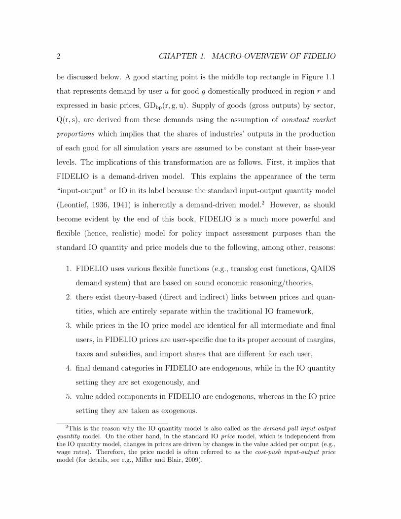
be discussed below. A good starting point is the middle top rectangle in Figure 1.1
that represents demand by user u for good g domestically produced in region r and
expressed in basic prices, GDbp(r, g, u). Supply of goods (gross outputs) by sector,
Q(r, s), are derived from these demands using the assumption of constant market
proportions which implies that the shares of industries’ outputs in the production
of each good for all simulation years are assumed to be constant at their base-year
levels. The implications of this transformation are as follows. First, it implies that
FIDELIO is a demand-driven model. This explains the appearance of the term
“input-output” or IO in its label because the standard input-output quantity model
(Leontief, 1936, 1941) is inherently a demand-driven model.2 However, as should
become evident by the end of this book, FIDELIO is a much more powerful and
flexible (hence, realistic) model for policy impact assessment purposes than the
standard IO quantity and price models due to the following, among other, reasons:
1. FIDELIO uses various flexible functions (e.g., translog cost functions, QAIDS
demand system) that are based on sound economic reasoning/theories,
2. there exist theory-based (direct and indirect) links between prices and quan-
tities, which are entirely separate within the traditional IO framework,
3. while prices in the IO price model are identical for all intermediate and final
users, in FIDELIO prices are user-specific due to its proper account of margins,
taxes and subsidies, and import shares that are different for each user,
4. final demand categories in FIDELIO are endogenous, while in the IO quantity
setting they are set exogenously, and
5. value added components in FIDELIO are endogenous, whereas in the IO price
setting they are taken as exogenous.
2This is the reason why the IO quantity model is also called as the demand-pull input-outputquantity model. On the other hand, in the standard IO price model, which is independent fromthe IO quantity model, changes in prices are driven by changes in the value added per output (e.g.,wage rates). Therefore, the price model is often referred to as the cost-push input-output pricemodel (for details, see e.g., Miller and Blair, 2009).

3
However, it is important to note that supply-side shocks can be simulated as well,
though FIDELIO fits better for the analysis of demand-side shocks.
FIDELIO shows several similarities with computable general equilibrium (CGE)
models, partly mentioned above in the five points where it was shown that FIDELIO
has a richer potential for policy impact assessment than the static IO model, but
also deviates from specifications in CGE models in some important aspects. In FI-
DELIO the supply side is specified in the dual model, i.e., a cost function that also
comprises total factor productivity (TFP). The output firms are supplying is in the
dual model with constant returns to scale determined by the demand side. Supply
side aspects come into play, as cost factors and prices determine the level of demand.
The growth of TFP is the most important long-term supply side force in that sense
in FIDELIO. As described in Kratena and Streicher (2009), the differences between
econometric IO modeling and CGE modeling have often been exaggerated and can in
many cases be reduced to certain features in the macroeconomic closure rules of the
models. This view can be upheld, when it comes to the differentiation of FIDELIO
from a dynamic CGE model, like the IGEM model for the U.S. economy (Goettle
et al., 2007).3 In CGE it is the changes in prices that bring about equilibrium in all
markets. In FIDELIO, however, the equilibrium concept in all markets is based on
the observed empirical regularities indicating how economies are evolving over time.
It is obvious that, in general, the base-year data, used in CGE and other modeling
frameworks, are not consistent with the concept of “economic equilibrium” in its
strict economic sense. Equilibrium is given in FIDELIO by demand reactions at
all levels of users and all types of goods or factor inputs, and by the corresponding
supply that is determined under the restrictions given at factor markets. The latter
are mainly represented by an exogenous benchmark interest rate and liquidity con-
straints, as far as the input of capital is concerned, and by the institution of union
3The complete description and applications of the IGEM model are available at http://www.
igem.insightworks.com/.
4 CHAPTER 1. MACRO-OVERVIEW OF FIDELIO
wage bargaining at industry level, as far as the input of labour is concerned. Savings
in the economy (domestic plus external) are not fixed by a fixed current account
balance, but are determined in the buffer stock model of consumption, taking into
account the wealth position (and therefore also the foreign wealth) of households.
Current and lagged household income has an impact on private consumption, as
far as lending constraints in the capital market are present and the purchase of
consumer durables cannot be fully financed by borrowing.
The public sector in the current version is specified with exogenous expen-
diture and therefore no explicit restriction on this balance for equilibrium in the
economy is integrated into FIDELIO. Anyway, for the construction of a ‘baseline’
scenario growth rates of transfer payments and public consumption in the different
countries that are ex ante in line with their mid-term fiscal stabilization targets (for
net lending and public debt as percentage of GDP) are taken into account. This
specification could easily be changed into an explicit restriction by endogenizing
transfer payments and public consumption, given the target path of net lending as
percentage of GDP.
Given the level of production Q(r, s) and input prices, firms are assumed to
minimize their total costs. Input prices are taken as given in this stage because
of perfect competition assumption. Further, with a constant returns to scale as-
sumption, minimization of total costs at given level of output becomes equivalent
to the minimization of a unit or average cost function, which represents the gross
output price by sector, PQ(r, s). Using the translog cost approach (see Chapter 2.2.2
for details), the derived input demands for five aggregate inputs are fist obtained.
These are demands for total energy inputs E(r, s), total domestic non-energy inputs
D(r, s), total imported non-energy inputs M(r, s) and demands for two primary in-
puts of labour L(r, s) and capital K(r, s). Aggregate labour is further disaggregated
into demands for three skill types: high-, medium- and low-skilled labour demands

5
Fig
ure
1.1
:O
verv
iew
ofth
em
ain
econ
omic
flow
sin
FID
EL
IO
Th
eva
riab
les
incl
ud
edw
ith
inre
dre
ctan
gles
are
end
ogen
ou
sva
riab
les.
Th
em
ain
fun
ctio
nal
form
san
dap
pro
ach
esu
sed
for
the
der
ivati
on
ofva
riou
sp
arts
ofth
em
od
elar
em
enti
oned
wit
hin
the
blu
eov
al
shap
es.
6 CHAPTER 1. MACRO-OVERVIEW OF FIDELIO
denoted, respectively, as LH(r, s), LM(r, s) and LL(r, s). Here also the translog cost
approach is employed, where the cost function is the wage earned per hour that
determines labour price PL(r, s) (pricing details are discussed below).
The next step is computing demands for intermediate goods at purchasers’
prices, Gpp(r, g, s). This is done by allocating the aggregate intermediate inputs
E(r, s), D(r, s) and M(r, s) over all goods g using the corresponding product use
structure (proportions) of the base year. Here, again if one expects that, for example,
the product structure of energy inputs proportions are going to be different in the
future compared to those in the base year, the corresponding information can be
exogenously incorporated in the corresponding structure matrix.
The derived input demand (and supply) of labour and capital make up the
total value added by sector, i.e., VA(r, s) = L(r, s) + K(r, s). At this stage also more
components of value added (i.e., wages, social security contributions, production
taxes and subsidies, and depreciation) are obtained, which we do not discuss here.
Regional public consumption demand and regional non-profit institutions serving
households (NPISH) consumption demand, both at purchasers’ prices, are currently
treated as exogenous. For the construction of a ‘baseline’ scenario these final de-
mand components are extrapolated according the regional targets for public net
lending. In a future version of FIDELIO, NPISH will be included in private con-
sumption and public consumption will be endogenized in a form that the net lending
targets are met explicitly. The corresponding totals for regional public consump-
tion demand and regional non-profit institutions serving households (NPISH) are
again distributed over all goods g employing the corresponding use structures of the
benchmark year, which results in the public and NPISH consumption demands for
products at purchasers’ prices, i.e., Gpp(r, g, gov) and Gpp(r, g, npish), respectively.
(The last are not shown in Figure 1.1 as currently they are exogenous.)
In FIDELIO it is recognized that private consumption is the largest compo-
7
nent of aggregate demand, and as such its modeling should be given a very care-
ful consideration. Obtaining private consumption demands at purchasers’ prices,
Gpp(r, g, con), consists of three stages. The first stage is based on a theory of inter-
temporal optimization of households with buffer stock saving as proposed by Luengo-
Prado (2006) and also discussed in Chapter 2.1.1. This theory takes into account
that households cannot optimize according to the permanent income hypothesis
due to credit market restrictions (liquidity constraints) and down payments for the
purchase of durables. From the optimality conditions of the intertemporal prob-
lem we derive policy functions of durable and nondurable consumption that turn
out to depend on households’ wealth, down payment requirement (needed for pur-
chasing durable goods) and the user cost of durables. The last in its turn depends
on durables’ prices, depreciation rates and the interest rate relevant to households’
durables purchases. This theory is used to compute the regional demands for four
durable commodities Appliances, Vehicles, Video and Audio, and Housing, and one
aggregate non-durable commodity. Demand for housing is derived not exactly in the
same way as the other three durables’ demands, because housing consists of owner
occupied houses and houses for rent, where the last is explained by demography
(these details are given in Chapter 4.4.1). In the second stage, the derived aggre-
gate nondurable demand is split up into its different components using the Quadratic
Almost Ideal Demand System (QAIDS) proposed by Banks, Blundell and Lewbel
(1997), which is also discussed in Chapter 2.1.2. Finally, the obtained demands
for durable and nondurable commodities consistent with COICOP classification4
are transformed into private consumption demands for products that are consistent
with CPA 2002 classification,5 Gpp(r, g, con), using the corresponding region-specific
4COICOP stands for “Classification of Individual Consumption According to Purpose”; see theUnited Nations Statistics Division’s COICOP information at http://unstats.un.org/unsd/cr/registry/regcst.asp?Cl=5.
5CPA stands for “Classification of Products by Activity”, for details see the Eurostat’s CPAinformation at http://ec.europa.eu/eurostat/ramon/nomenclatures/index.cfm?TargetUrl=LST_NOM_DTL&StrNom=CPA&StrLanguageCode=EN&IntPcKey=&StrLayoutCode=HIERARCHIC.

8 CHAPTER 1. MACRO-OVERVIEW OF FIDELIO
bridge matrices between the two systems.
Sectoral capital stocks KS(r, s) are obtained from the assumption that their
total user cost value is equal to the sectoral capital compensation (cash flow). Two
options of static and dynamic concepts of user cost of capital can be employed, both
of which assume that capital market is in equilibrium in each period (Jorgenson,
1967; Christensen and Jorgenson, 1969). User cost of capital depends on price of
investments, interest rate for capital costs of firms’ purchases and depreciation rate
by industry (see Chapter 4.4.3). Then using Leontief technology, in this case the
base-year investment-to-capital stock proportions, the investment demand by sector
in purchasers’ prices INVpp(r, s) is obtained. These are finally transformed into
the investment demands for products at purchasers’ prices Gpp(r, g, inv) using the
benchmark-year product structure of investments.
Demands for exports in purchasers’ prices Gpp(r, g, u) are obtained from the
endogenous trade flows between the model regions (which in Figure 1.1 is denoted
as TRDM(r, rt, g, u) and indicates region r’s demands for imports from its trade
partner rt) plus the exports to the rest of the world. The last component of final
demand – demand for inventory – is assumed to be fixed at its base-year use level for
all products, and for this reason is not given in the middle-right square of Figure 1.1
that includes four endogenous components of final demand. These are all demands
for both domestically produced and imported goods (or composite goods, for short).
Taking into account trade and transport margins and taxes less subsidies on prod-
ucts, these purchasers’ price demands are translated into the demands for composite
goods at basic prices Gbp(r, g, u), the details of which are given in Chapter 4.5.
Multiplication of total import shares MSH(r, g, f) by the corresponding basic
price demands for composite goods Gbp(r, g, f) gives final user f ’s demand in region
r for total imported good g valued at CIF prices, IMP(r, g, f). Sectoral demand
for intermediate imports of energy goods IMP(r, ge, s) is derived similarly, but that
9
for non-energy good IMP(r, gne, s) is obtained differently, namely, by multiplica-
tion of the total demand for non-energy imported inputs (from the Translog model
of factor demands) with the use-structure matrix for imported non-energy inter-
mediates. This use-structure matrix and the total import shares are assumed to
be the same as those of the base year for all users, except for private consumers
where the Armington approach is applied (i.e., the total import shares of consumers
MSH(r, g, con) depend on domestic and import prices). The partner-specific import
demands TRDM(r, rt, g, u) are computed from the total imports demand IMP(r, g, u)
using the base-year trade shares in combination with the Armington approach (for
details, see Chapter 4.6).
And finally, deducting imports IMP(r, g, u) from demands for composite goods
at basic prices Gbp(r, g, u) gives demand for domestically produced goods in basic
prices, GDbp(r, g, u), with which we have started the brief explanation of the main
economic flows demonstrated in Figure 1.1. This closes the loop of the main flows
interactions with the understanding that quite crucial details behind these dependen-
cies are skipped for simplicity purposes and are discussed in the following chapters.
We now turn to the discussion of various prices (but not all prices, similar to
the flows discussion above), which naturally affect directly and/or indirectly all the
endogenous variables discussed so far. The derivation of all the prices is discussed
in Chapter 4.8, while the required theoretical reasonings are presented in the next
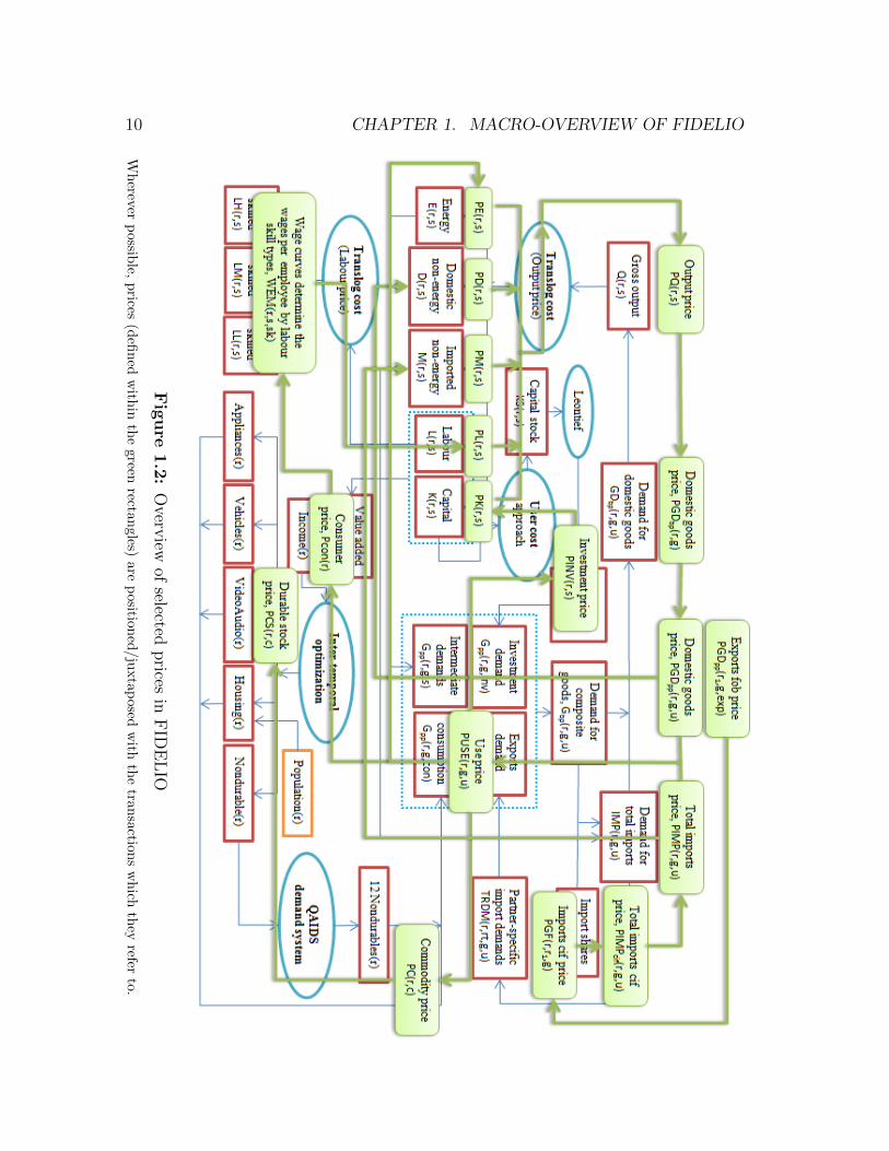
chapter. The overview of the main prices are illustrated in Figure 1.2, where prices
are juxtaposed on the flows chart of Figure 1.1. Wherever possible, prices are
positioned close to the transactions which they refer to.
Let us start with the gross output prices PQ(r, s) that are basic prices deter-
mined, through the translog cost approach, from the prices of energy inputs PE(r, s),
of domestic non-energy inputs PD(r, s), of imported non-energy inputs PM(r, s), of
labour PL(r, s), and of capital PK(r, s), and time (in order to take into account
10 CHAPTER 1. MACRO-OVERVIEW OF FIDELIO
Fig
ure
1.2
:O
verview
ofselected
prices
inF
IDE
LIO
Wh
ereverp
ossible,
prices
(defi
ned
with
inth
egreen
rectan
gles)
are
positio
ned
/ju
xta
posed
with
the
transaction
sw
hich
they
referto.
11
the effect of technical progress due to TFP growth in the unit cost function and
factor-biased technical progress). The last five mentioned prices also enter in the
derivation of derived demands for aggregate inputs.
Basic prices of domestic products PGDbp(r, g) are obtained as weighted aver-
ages of the sectoral gross output prices, where the base-year market shares of sectors
are used as weights. Note that the last price is the same for all users, similar to
the standard IO price model. However, taking into account the fact that in pur-
chasers’ prices, demand for products is essentially demand for a composite good, i.e.,
the good itself, trade and transport margins, and taxes less subsidies on the good,
the purchaser prices of domestically produced products PGDpp(r, g, u) become user-
specific. The FOB price of exports in the exporter region r1 is PGDpp(r1, g, exp),
which once corrected for the exchange rates and augmented by international trans-
port costs and tariffs gives the CIF prices at the border of the importing region r
for goods imported from region r1, PGF(r, r1, g). The corresponding CIF prices for
imports from the rest of the world PGF(r, row, g) are taken exogenous to the model.
Next, the weighted average of the import prices of trading partners (i.e.,
PGF’s) gives the total import CIF price at the border of region r for good g and
user u, PIMPcif(r, g, u), where the endogenously determined trading partner-specific
import shares are taken as weights. Further accounting for domestic markups turn
PIMPcif(r, g, u) into the total import prices including domestic margins and taxes
less subsidies on products, PIMP(r, g, u).
Products’ use prices for intermediate and final users PUSE(r, g, u) are the
weighted averages of the purchasers’ prices of domestic products PGDpp(r, g, u) and
import prices PIMP(r, g, u) using the import shares MSH(r, g, u) as the correspond-
ing weights. The aggregate price of energy inputs PE(r, s) is determined using the
base-year product structure of energy inputs and the corresponding sectoral use
prices PUSE(r, g, s). Similarly, combining the purchasers’ prices of domestic goods

12 CHAPTER 1. MACRO-OVERVIEW OF FIDELIO
PGDpp(r, g, u) (resp. the import prices PIMP(r, g, u)) with the base-year product
structure of domestic (resp. imported) non-energy inputs results in the aggregate
prices of domestic (resp. imported) non-energy inputs PD(r, s) (resp. PM(r, s)). By
the same principle, the prices of investments PINV(r, s) are determined from the
products’ use prices for investments and the base-year product structure of invest-
ments.
The regional use price for each user is the aggregate price of “inputs” for that
user, and is obtained as the weighted average of the corresponding use prices with
weights representing the product shares of endogenously derived demands for goods
in purchasers’ prices. If the user is private consumer, then the corresponding regional
use price is the consumer price, Pcon(r). Using the COICOP-CPA bridge matri-
ces of the base year, products’ use prices for private consumption PUSE(r, g, con)
are translated into the prices of durable and nondurable consumption commodities
PC(r, c). The prices of stocks of durable commodities PCS(r, c) are obtained using
the concept of user cost of durable goods.
The wages per employee of the high-, medium- and low-skilled labour, de-
noted respectively as WEM(r, s, high), WEM(r, s,med) and WEM(r, s, low), are de-
termined by wage curves (Blanchflower and Oswald, 1994; see also Chapter 2.3.2),
which in FIDELIO relate labour skill type wages to labour productivity, consumer
price and skill-specific unemployment rates. These wages together with time com-
ponents (in order to take into account the effects of technical change in the aggre-
gate wage rate function and skill-biased technical progress) within the translog cost
framework determine average wage earned per hour, which in turn defines the price
of labour PL(r, s). Finally, the price of sectoral capital stock PK(r, s) is obtained
from the investments prices PINV(r, s) using the notion of the user cost of capital.
By now it should, in principle, become clear why the model is called Fully
Interregional Dynamic Econometric Long-term Input-Output (FIDELIO) model. It
13
is “fully interregional” because it is a complete inter-regional economic model that
takes into account the most important features (for policy analysis purposes) of con-
sumption, production, labour market, trade between regions, and the environment.
However, the full-fledged environmental block is (still) not discussed in this book,
keeping in mind that some simple environmental impact calculations are straightfor-
ward to make once production- and consumption-side impacts are obtained from the
model. The quantity and price interactions between regions (currently 27 EU Mem-
ber States and one rest of the world region) are taken into account by comprehensive
modeling of interregional trade flows. It is “dynamic” because, as mentioned above,
the consumption block is based on an inter-temporal optimization approach and
capital stocks (and investments) derivation is based on dynamic neoclassic theory of
optimal capital accumulation. Further, time is explicitly included in the derivations
of prices and firms’ demands for intermediate and primary inputs, while various
lagged flow and price variables are contained in the consumption demands. These
ultimately lead the model to be inherently a dynamic model in the sense of its over-
time policy impact assessment capability. The model is “econometric” because the
crucial parameters’ values in the functions, characterizing economic agents’ reactions
in consumption, production and labour blocks, are estimated from the appropriate
time series data employing most relevant (advanced) econometric techniques. The
model is “long-term” because the durable and nondurable consumption demands
are expressed in the form of long-run equilibrium relationships of an error correc-
tion model specification. This allows computing not only short-run effects, but also
long-run equilibrium effects and the adjustment speeds of the short-run deviations
toward the long-run equilibrium. Finally, the “input-output” part has been already
explained in the beginning of this chapter. Here, it additionally needs to be noted
that detailed supply and use tables make the core data of FIDELIO, which constitute
the building blocks of the commodity-industry approach in input-output analysis.

14 CHAPTER 1. MACRO-OVERVIEW OF FIDELIO

Chapter 2
Theoretical foundations of
FIDELIO
2.1 Consumption block
Since private consumption is by far the largest component of aggregate demand, it
is of utmost importance to pay special attention to consumption behavior model-
ing. The consumption block of FIDELIO consists of two nests. First, households’
demands for four types of durable and one aggregate non-durable commodities are
derived, and then the aggregate nondurables obtained from the first step is split into
its different categories. The theories behind these steps are explained below.
2.1.1 Households’ demands for four types of durable and
total non-durable commodities
This part of FIDELIO’s consumption block is based on a theory of inter-temporal
optimization problem of households along the lines of the ‘buffer stock model’ of
15
16 CHAPTER 2. THEORETICAL FOUNDATIONS OF FIDELIO
consumption. The traditional way of linking a consumption block to an input-
output (IO) model is the social accounting matrix (SAM) multiplier model, where
the accounts for household income are linked to value added on the one side and
to consumption on the other side. This specification is based on the Keynesian
theory of consumption, and consumption mainly depends on current disposable
income. There is – to our knowledge – only one attempt in the literature to link
the IO model to a dynamic model of consumption, based on the permanent income
hypothesis, namely Chen et al. (2010). However, the permanent income hypothesis
has been challenged by different empirical puzzles that show a certain dependence
of household consumption on current household income. This has been motivated
by the existence of liquidity constraints and ‘buffer stock’ savings behavior in order
to build up reserves for unexpected events and expenditure. Carroll (1997) has
laid down the base of the buffer stock model, starting from the empirical puzzles
that the permanent income hypothesis was not able to resolve. In FIDELIO we
use a form of the buffer stock model, where households save for the purchase of
durables, as described in Luengo-Prado (2006). Consumers maximize the present
discounted value of expected utility from consumption of nondurable commodity Ct
and from the service flow provided by the stocks of durable commodity Kt, subject
to the budget and collateralized constraints. A very crucial and novel feature of
this model is consideration of the last constraint imposed on consumers. It includes
the so-called down payment requirement parameter, θ ∈ [0, 1], which represents the
fraction of durables that a household is not allowed to finance. Hence, the borrowing
limit (or maximum loan) of an individual is equal to (1− θ) fraction (share) of the
stocks of durable commodities. The mentioned constraint then implies that, at any
point in time, the household is only required to keep an accumulated durable equity
equal to θKt, i.e., to θ fraction of the stocks of durable commodities.
Without going into all the mathematical details of the mentioned problem, we

2.1. CONSUMPTION BLOCK 17
will just briefly discuss the main results of Luengo-Prado’s (2006) paper. Using the
same notation, the interest and depreciation factors are denoted, respectively, by
R ≡ 1 + r and ψ ≡ 1− δ, where r and δ are the rates of interest and depreciation,
respectively. Then (R−ψ)/R = (r+δ)/(1+r) is known as the user cost of the durable,
or rental equivalent cost of one durable unit. The dependence of user cost on interest
and depreciation rates has the following reasoning. The user cost increases if the
interest rate r goes up because then the opportunity cost of investing in the durable
increases: an euro invested in the durable commodity would have given a return of
r if invested in financial assets. It is also evident that the higher depreciation erodes
consumers’ investments in the durable, which is equivalent to increasing the cost of
using such a durable.
The following definitions will be useful. First, cash-on-hand is defined as the
sum of assets holding, stocks of durables and income, i.e., Xt ≡ (1 + r)At−1 + (1−
δ)Kt−1 + Yt. Total wealth of a household, At + Kt, is comprised of the required
down payment, θKt, and voluntary equity holding, Qt ≡ At + (1− θ)Kt. Using these
definitions and the budget constraint At = (1+r)At−1+Yt−Ct−(Kt−(1−δ)Kt−1), it
can be readily seen that the difference between cash-on-hand and voluntary equity
holding is the sum of nondurable consumption and down payment share of the
durable stock consumption, i.e.,
Xt −Qt = Ct + θKt. (2.1)
The analysis then proceeds with normalized variables, where all the variables
are divided by permanent income, in order to deal with the nonstationarity of in-
come, as proposed by Carroll (1997). As far as the collateralized constraint is
concerned, two cases should be distinguished:
(i) Constrained agents: the normalized cash-on-hand, x, is below the unique
threshold level, x∗(θ) ≡ c + θk, when the agent will be left without any re-
18 CHAPTER 2. THEORETICAL FOUNDATIONS OF FIDELIO
sources once she pays for nondurable consumption and the down payment
requirement. Here, thus no voluntary equity is carried over to the next period,
i.e., q = a+ (1− θ)k = 0.
(ii) Non-constrained agents: normalized cash-on-hand is higher than x∗(θ), hence
some voluntary equity is accumulated, i.e., q > 0.
Luengo-Prado (2006) derives the policy functions of durable and nondurable
consumption that turn out to be a function of the difference of cash-on-hand and
voluntary equity holding, xt − qt, down payment parameter, θ, and
Ω ≡ ϕ−1/ρ
[r + δ
1 + r
]1/ρ
, (2.2)
where ϕ and ρ are consumer’s preference parameters with ρ > 0 implying risk-averse
agent with precautionary motive for saving. Note that the expression in brackets
in (2.2) is the user cost of the durable. Let us now discuss the main results of
Luengo-Prada (2006) that are relevant for FIDELIO.
First, for nonconstrained agents, i.e., when xt > x∗t (θ), irrespective of the value
of down payment parameter, θ, it must be the case that ct/kt = Ct/Kt = Ω, where
the policy functions take the following forms:
ct =Ω
Ω + θ(xt − qt), (2.3)
kt =1
Ω + θ(xt − qt). (2.4)
That is, when the collateralized constrained is not binding, once the agent decides
on her voluntary equity to be kept on to the next period, she simply spends fixed
proportions of the cash-on-hand leftover between the durable and nondurable com-
modities.
The richness of the model, however, becomes apparent when one considers the
second case of constrained agents with xt ≤ x∗t (θ). Here everything depends on the
2.1. CONSUMPTION BLOCK 19
value of θ and, crucially, its link to the user cost term. In particular, Proposition 2
in Luengo-Prado (2006) proves that:
(i) if θ = 0, then ct = xt and kt = (1/Ω)x∗(θ),
(ii) if θ < (R−ψ)/R, then ct (resp. kt) is a convex (resp. concave) function of xt,
(iii) if θ = (R − ψ)/R, then the policy function are linear: ct = [Ω/(Ω + θ)]xt and
kt = [1/(Ω + θ)]xt, and
(iv) if (R − ψ)/R < θ ≤ 1, then ct (resp. kt) is a concave (resp. convex) function
of xt.
The policy functions in all the above considered cases are illustrated in Fig-
ure 2.1. It turns out that all this flexibility of the derived policy functions (in terms
of their curvature and flatness) makes the model capable of explaining such concepts
in macroeconomics as excess smoothness and excess sensitivity observed in US and
other countries’ aggregate data. These were puzzling observations because they were
not in line with the predictions of the life cycle-permanent income hypothesis that
states that consumption is determined by the expected value of lifetime resources
or permanent income. Excess smoothness refers to the empirical observations that
consumption is excessively smooth, i.e., consumption growth is smoother than per-
manent income. It has been also found that consumption is excessively sensitive:
Ct+1 reacts to date t or earlier variables other than Ct (for example, income at
time t), whereas the standard inter-temporal optimization condition would state
that it should not (Hall, 1978, is the pioneering work in this field) because all past
and predictable information is already incorporated in current consumption so that
no lagged information can provide additional explanatory power in accounting for
variations in future consumption. It is important to realize that consumption can
simultaneously display excess sensitivity and excess smoothness. This is because
excess sensitivity refers to how consumption reacts to past, thus predictable, income

20 CHAPTER 2. THEORETICAL FOUNDATIONS OF FIDELIO
c=x-q
c=x
1
x*
x*Ω
1(x-q)
Ωk=
k=
45º
q=0 x x*
1(x-q)
(Ω+θ)k=
45º
q=0 x
Ω(x-q)
(Ω+θ)c=
x*
1(x-q)
(Ω+θ)k=
45º
q=0 x
Ω(x-q)(Ω+θ)c=
x*
1(x-q)
(Ω+θ)k=
45º
q=0 x
Ω(x-q)
(Ω+θ)c=
(a) Case 1: θ = 0 (b) Case 2: 0 < θ < (R-ψ)/R
(c) Case 3: θ = (R-ψ)/R (d) Case 4: (R-ψ)/R < θ < 1
Figure 2.1: Policy functions. Durable and nondurable as a function of cash-on-hand
shocks whereas excess smoothness refers to how consumption reacts to present, thus
unpredictable, income shocks.
From Figure 2.1 it follows, for example, that for a constrained household as the
down payment requirement increases, the policy function for the nondurable com-
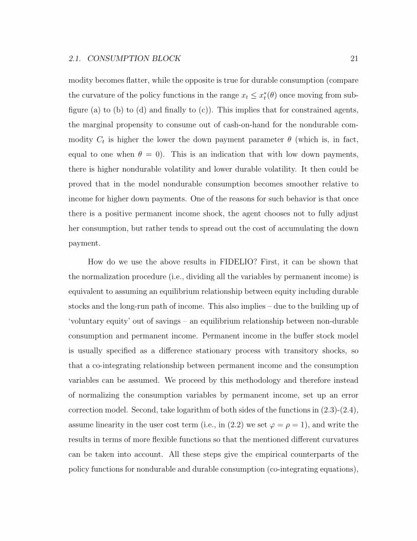
2.1. CONSUMPTION BLOCK 21
modity becomes flatter, while the opposite is true for durable consumption (compare
the curvature of the policy functions in the range xt ≤ x∗t (θ) once moving from sub-
figure (a) to (b) to (d) and finally to (c)). This implies that for constrained agents,
the marginal propensity to consume out of cash-on-hand for the nondurable com-
modity Ct is higher the lower the down payment parameter θ (which is, in fact,
equal to one when θ = 0). This is an indication that with low down payments,
there is higher nondurable volatility and lower durable volatility. It then could be
proved that in the model nondurable consumption becomes smoother relative to
income for higher down payments. One of the reasons for such behavior is that once
there is a positive permanent income shock, the agent chooses not to fully adjust
her consumption, but rather tends to spread out the cost of accumulating the down
payment.
How do we use the above results in FIDELIO? First, it can be shown that
the normalization procedure (i.e., dividing all the variables by permanent income) is
equivalent to assuming an equilibrium relationship between equity including durable
stocks and the long-run path of income. This also implies – due to the building up of
‘voluntary equity’ out of savings – an equilibrium relationship between non-durable
consumption and permanent income. Permanent income in the buffer stock model
is usually specified as a difference stationary process with transitory shocks, so
that a co-integrating relationship between permanent income and the consumption
variables can be assumed. We proceed by this methodology and therefore instead
of normalizing the consumption variables by permanent income, set up an error
correction model. Second, take logarithm of both sides of the functions in (2.3)-(2.4),
assume linearity in the user cost term (i.e., in (2.2) we set ϕ = ρ = 1), and write the
results in terms of more flexible functions so that the mentioned different curvatures
can be taken into account. All these steps give the empirical counterparts of the
policy functions for nondurable and durable consumption (co-integrating equations),
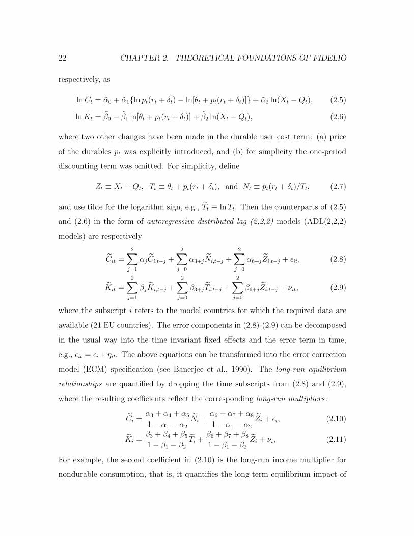
22 CHAPTER 2. THEORETICAL FOUNDATIONS OF FIDELIO
respectively, as
lnCt = α0 + α1ln pt(rt + δt)− ln[θt + pt(rt + δt)]+ α2 ln(Xt −Qt), (2.5)
lnKt = β0 − β1 ln[θt + pt(rt + δt)] + β2 ln(Xt −Qt), (2.6)
where two other changes have been made in the durable user cost term: (a) price
of the durables pt was explicitly introduced, and (b) for simplicity the one-period
discounting term was omitted. For simplicity, define
Zt ≡ Xt −Qt, Tt ≡ θt + pt(rt + δt), and Nt ≡ pt(rt + δt)/Tt, (2.7)
and use tilde for the logarithm sign, e.g., Tt ≡ lnTt. Then the counterparts of (2.5)
and (2.6) in the form of autoregressive distributed lag (2,2,2) models (ADL(2,2,2)
models) are respectively
Cit =2∑j=1
αjCi,t−j +2∑j=0
α3+jNi,t−j +2∑j=0
α6+jZi,t−j + εit, (2.8)
Kit =2∑j=1
βjKi,t−j +2∑j=0
β3+jTi,t−j +2∑j=0
β6+jZi,t−j + νit, (2.9)
where the subscript i refers to the model countries for which the required data are
available (21 EU countries). The error components in (2.8)-(2.9) can be decomposed
in the usual way into the time invariant fixed effects and the error term in time,
e.g., εit = εi + ηit. The above equations can be transformed into the error correction
model (ECM) specification (see Banerjee et al., 1990). The long-run equilibrium
relationships are quantified by dropping the time subscripts from (2.8) and (2.9),
where the resulting coefficients reflect the corresponding long-run multipliers :
Ci =α3 + α4 + α5
1− α1 − α2
Ni +α6 + α7 + α8
1− α1 − α2
Zi + εi, (2.10)
Ki =β3 + β4 + β5
1− β1 − β2
Ti +β6 + β7 + β8
1− β1 − β2
Zi + νi, (2.11)
For example, the second coefficient in (2.10) is the long-run income multiplier for
nondurable consumption, that is, it quantifies the long-term equilibrium impact of

2.1. CONSUMPTION BLOCK 23
changes in income (cash-on-hand net of voluntary equity holding) on the household’s
demand for nondurable commodities.
Finally, if one writes (2.8) and (2.9) in the ECM form, then it immediately
becomes evident that the error-correction parameters in the corresponding equations
equal, respectively,
− (1− α1 − α2) and − (1− β1 − β2), (2.12)
which determine the speed of adjustment towards the long-run equilibrium.
The error correction models equivalent to the ADL (2,2,2) models in (2.8)
and (2.9) have been estimated using the GMM estimator for dynamic panel data
proposed by Blundell and Bond (1998). The estimates of all the coefficients, error-
correction parameters (ECP ) and the long-run ‘durable cost’1 and income multipli-
ers (M1 and M2, respectively) are presented in the table below.
Table 2.1: Parameters for computing the durable and nondurable demands
Nondurables α1 α2 α3 α4 α5 α6 α7 α8 ECP M1 M2
Aggregate 1.277 -0.432 0.063 0.059 -0.099 0.185 -0.534 0.422 -0.155 0,153 0.472
Durables β1 β2 β3 β4 β5 β6 β7 β8 ECP M1 M2
VideoAudio 1.585 -0.660 -0.107 0.104 -0.015 0.095 -0.124 0.076 -0.075 -0.244 0.632
Vehicles 1.771 -0.859 -0.261 0.458 -0.162 0.090 -0.312 0.250 -0.088 0.404 0.321
Appliances 1.619 -0.677 -0.075 0.077 -0.017 0.025 -0.036 0.023 -0.058 -0.259 0.193
Housing 1.840 -1.098 0.677 -0.168 -0.675 -0.710 0.637 0.283 -0.259 -0.643 0.812
Note: ECP = error correction parameter in (2.12), M1 and M2 are the long-run durable cost and income multipliers
in (2.10) and (2.11).
The results in Table 2.1 show, for example, that the adjustment speed to
long-run equilibrium is highest for Housing and lowest for Appliances, which also
have, respectively, the biggest and lowest income long-run multipliers, M2. Note
1These have different interpretations for Ct and Kt: for nondurables, it is the elasticity ofconsumption demand with respect to the share of the durable user cost in the user cost plus downpayment requirement, pt(rt + δt)/[θt + pt(rt + δt)], and for durables, these are the elasticities ofconsumption demand with respect to the durable user cost plus the down payment requirement.

24 CHAPTER 2. THEORETICAL FOUNDATIONS OF FIDELIO
that the stocks of vehicles, video/audio, appliances and housing variables are in cur-
rent prices, therefore a long-run multiplier M1 < 1 guarantees a negative own price
elasticity. This reasoning does not apply to non-durables, as the corresponding mul-
tiplier M1 measures cross-price elasticity (i.e., reaction of non-durable consumption
to durable costs) and therefore any positive value guarantees a substitution effect.
2.1.2 Splitting aggregate nondurable commodity into its dif-
ferent categories
Once consumption of total nondurable commodity has been estimated using the
approach discussed in Chapter 2.1.1, we need to split up this aggregate demand
into its different components.2 For the purposes of this second step allocation the
so-called Quadratic Almost Ideal Demand System (QAIDS) proposed by Banks,
Blundell and Lewbel (1997) is used. This model is quite popular and widely-used
approach in applied microeconomics for estimating demand functions. Therefore,
without going into all the details, the main result is that the expenditure share
equation for the i-th nondurable commodity of a utility-maximizing consumer has
the following form:
wi = αi +∑j
γij ln pj + βi ln
[C
a(p)
]+
λib(p)
ln
[C
a(p)
]2
, (2.13)
where wi is the expenditure share of nondurable commodity i, p = (p1, p2, . . . , pn)′
is the vector of prices of the n nondurable commodities, a(p) is the price index used
to deflate nominal aggregate consumption C to arrive at real total expenditure,
b(p) is another price index reflecting the cost of bliss (within AIDS model), and
2As pointed out by Attanasio and Weber (1995, p. 1144), this strategy is consistent with atwo step interpretation of the intertemporal optimization problem: in the first step, the consumerdecides how to allocate expenditure across time periods, while in the second step, she allocates thederived expenditure for each time period to its different consumption categories. This second stepallocation depends on the prices of consumption categories and the corresponding total expenditure.
2.1. CONSUMPTION BLOCK 25
the rest are parameters to be estimated. If λi = 0, then (2.13) reduces to the
AIDS model of Deaton and Muellbauer (1980). Thus, the AIDS model assumes
that demand (or expenditure share) equations are linear in log of real income, but
its extension – QAIDS allows for non-linear Engel curves that could be observed for
some commodities in practice (e.g., alcohol and clothing).
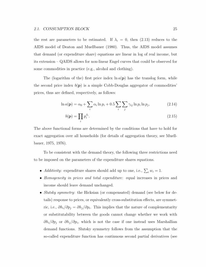
The (logarithm of the) first price index ln a(p) has the translog form, while
the second price index b(p) is a simple Cobb-Douglas aggregator of commodities’
prices, thus are defined, respectively, as follows:
ln a(p) = α0 +∑i
αi ln pi + 0.5∑i
∑j
γij ln pi ln pj, (2.14)
b(p) =∏i
pβii . (2.15)
The above functional forms are determined by the conditions that have to hold for
exact aggregation over all households (for details of aggregation theory, see Muell-
bauer, 1975, 1976).
To be consistent with the demand theory, the following three restrictions need
to be imposed on the parameters of the expenditure shares equations.
• Additivity : expenditure shares should add up to one, i.e.,∑
iwi = 1.
• Homogeneity in prices and total expenditure: equal increases in prices and
income should leave demand unchanged.
• Slutsky symmetry : the Hicksian (or compensated) demand (see below for de-
tails) response to prices, or equivalently cross-substitution effects, are symmet-
ric, i.e., ∂hi/∂pj = ∂hj/∂pi. This implies that the nature of complementarity
or substitutability between the goods cannot change whether we work with
∂hi/∂pj or ∂hj/∂pi, which is not the case if one instead uses Marshallian
demand functions. Slutsky symmetry follows from the assumption that the
so-called expenditure function has continuous second partial derivatives (see
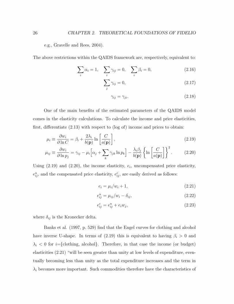
26 CHAPTER 2. THEORETICAL FOUNDATIONS OF FIDELIO
e.g., Gravelle and Rees, 2004).
The above restrictions within the QAIDS framework are, respectively, equivalent to:∑i
αi = 1,∑i
γij = 0,∑i
βi = 0, (2.16)
∑j
γij = 0, (2.17)
γij = γji. (2.18)
One of the main benefits of the estimated parameters of the QAIDS model
comes in the elasticity calculations. To calculate the income and price elasticities,
first, differentiate (2.13) with respect to (log of) income and prices to obtain:
µi ≡∂wi∂ lnC
= βi +2λib(p)
ln
[C
a(p)
], (2.19)
µij ≡∂wi∂ ln pj
= γij − µi[αj +
∑k
γjk ln pk
]− λiβjb(p)
ln
[C
a(p)
]2
. (2.20)
Using (2.19) and (2.20), the income elasticity, ei, uncompensated price elasticity,
euij, and the compensated price elasticity, ecij, are easily derived as follows:
ei = µi/wi + 1, (2.21)
euij = µij/wi − δij, (2.22)
ecij = euij + eiwj, (2.23)
where δij is the Kronecker delta.
Banks et al. (1997, p. 529) find that the Engel curves for clothing and alcohol
have inverse U-shape. In terms of (2.19) this is equivalent to having βi > 0 and
λi < 0 for i=clothing, alcohol. Therefore, in that case the income (or budget)
elasticities (2.21) “will be seen greater than unity at low levels of expenditure, even-
tually becoming less than unity as the total expenditure increases and the term in
λi becomes more important. Such commodities therefore have the characteristics of
2.1. CONSUMPTION BLOCK 27
luxuries at low levels of total expenditure and necessities at high levels” (Banks et
al., 1997, p. 534, emphasis added).
Recall from consumer theory that there are two demand curves which do not
respond identically to a price change. These are Marshallian demand (after the
economist Alfred Marshall, 1842–1924) and Hicksian demand (after the economist
John Richard Hicks, 1904–1989) curves. Marshallian demand quantifies how the
quantity of a commodity demanded change in response to the change of the price of
that commodity, holding income and all other prices constant. As such they com-
bine both the well-known (to economists) income and substitution effects of a price
change. Thus, Marshallian demand curves can be also called “net” demands be-
cause they aggregate the two conceptually distinct consumers’ behaviorial responses
to price changes.
Hicksian demand function, however, shows how the quantity demanded change
with a price of the good, holding consumer utility constant. But to hold consumer
utility constant (or keep the consumer on the same indifference curve) as prices
vary, adjustments to the consumer’s income are necessary, i.e., the consumer must be
compensated. Therefore, Hicksian demand is called “compensated” demand, and for
the analogous reason Marshallian demand is called “uncompensated” demand. The
Slutsky equation (2.23) is used to calculate the set of compensated price elasticities.
The parameters estimated from the QAIDS model, which are used in the
consumption block calibration of FIDELIO are given in Table 2.2. Note that the
reported estimates are provided for ten nondurables, where Energy includes Heat-
ing and Electricity, and Transport includes Private Transport and Public Transport.
Notice that all the presented estimates obey the additivity, homogeneity and sym-
metry restrictions given in (2.16), (2.17) and (2.18), respectively. And because of
the last restriction, for simplicity, we skip all the γij’s for all j > i. Also observe that
since the values of λi are almost all zero, then the AIDS specification of the linear

28 CHAPTER 2. THEORETICAL FOUNDATIONS OF FIDELIO
Tab
le2.2
:P
arameters
ofth
eQ
AID
Sm
odel
Non
du
rab
lei
Estim
ates
of
the
para
maters
in(2
.13),
(2.14)an
d(2.15)
αi
βi
λi
γi,1
γi,2
γi,3
γi,4
γi,5
γi,6
γi,7
γi,8
γi,9
γi,1
0
Food
0.4576
-0.1
0610.002
90.0
99
Alco
hol
0.0
756-0.00
400.00
01
0.0
22
0.0
16
Clo
thin
g0.10
33
-0.0055
0.0001
-0.0
25
-0.0
05
0.0
24
En
ergy0.06
86
-0.0
1570.00
04
-0.0
08
-0.0
06
-0.0
08
0.0
22
Tra
nsp
ort0.0
8670.0
144-0.00
04
-0.0
62
-0.0
05
0.0
06
0.0
04
0.0
50
Com
mu
nica
tion-0.028
40.02
08-0.000
60.0
06
0.0
01
-0.0
02
0.0
04
0.0
00-0.003
Recreatio
n0.0
279
0.0202
-0.0006
-0.0
05
-0.0
03
0.0
01
0.0
02
0.0
03-0.001
0.006
Hea
lth0.0
060
0.0
282-0.000
8-0
.008
0.0
05
0.0
01
-0.0
05
-0.0
03-0.001
0.0010.011
Hotels
&resta
uran
ts0.1
795
-0.0
0260.000
1-0
.024
-0.0
24
0.0
09
-0.0
11
0.0
120.000
-0.0020.000
0.038
Oth
ern
ond
urab
les0.023
10.05
02-0.001
40.0
06
0.0
00
-0.0
01
0.0
06
-0.0
05-0.004
-0.001-0.001
0.001-0.001
Su
m1.0
000
0.0
0000.00
00
0.0
00
-0.0
22
0.0
30
0.0
23
0.0
57-0.009
0.0030.010
0.040-0.001
Note
:S
ince
the
para
meters
γij
are
sym
metric,
for
simp
licityth
eestim
ates
ofγij
=γji
aresk
ipp
edfrom
the
table
forall
j>i.
Nu
mb
ersj
=1,2,...,1
0stan
dfor
the
non
du
rab
leco
mm
od
itiesacco
rdin
gto
the
ord
erap
pearin
gin
the
first
colum
nof
this
table,
e.g.,
1=
Food
,2
=A
lcoh
ol,
and
sofo
rthu
pto
10=
Oth
ern
on
du
rab
les.

2.2. PRODUCTION BLOCK 29
Engel curves for all nondurables seems not to contradict the data. In FIDELIO all
these parameters are assumed to be the same for all countries.
Energy and Transport now have to be split into Electricity and Heating, and
Private Transport and Public Transport, respectively. For this purpose, for energy
splitting first the following regression has been run:
Electricity share = c1 + c2 ln(Pelectricity/Pheating) + c3 ln(Energy/Penergy), (2.24)
where Pelectricity stands for the price of electricity. Note that (2.24) is nothing else
as the AIDS model for two nondurables Electricity and Heating, i.e., (2.13) without
its last term. It is given only for Electricity because Heating share will be derived
as a residual using the adding-up restriction. Similar approach has been used for
computing (calibrating) the share of Private Transport in total Transport, while
Public Transport is treated as the residual in this category. Table 2.3 shows the
estimates of the parameters for heating and public transport shares equations that
are used in FIDELIO for splitting Energy and Transport into their corresponding
two components.
Table 2.3: AIDS parameters for splitting Energy and Transport
Share of c1 c2 c3
Electricity in Energy 0.4216 0.0170 0.0052
Private Transport in Transport 0.8123 0.0537 0.1300
The estimates reported in Table 2.3 are assumed to be the same for all countries.
2.2 Production block
The production block of FIDELIO is based on cost minimization approach, where
the cost function has been chosen to have a flexible functional form known in the
30 CHAPTER 2. THEORETICAL FOUNDATIONS OF FIDELIO
literature as transendental logarithmic function, or translog function for short. In
applied econometrics flexible functional forms are used for the purpose of modeling
second-order effects (e.g., elasticities of substitution) that are functions of the second
derivatives of cost, utility or production functions. Given the importance of the
translog function, we first provide a brief overview of its derivation, and then discuss
FIDELIO nests of the production block.
2.2.1 The translog function
The most popular flexible functional form used in the empirical studies of production
is the translog function, which is interpreted as a second-order approximation of an
unknown function of interest. We provide a brief discussion of this function, while
for further details the reader is referred to Christensen, Jorgenson and Lau (1973),
Bernt and Christensen (1973), Christensen, Jorgenson and Lau (1975), Bernt and
Wood (1975), Christensen and Greene (1976), and Greene (2003).
Suppose the function is y = g(x1, x2, . . . , xn), which can be taken as ln y =
ln g(x1, x2, . . . , xn). But since xi = exp(lnxi), we can interpret the function of
interest as a function of the logarithms of xi’s, i.e., ln y = f(lnx1, lnx2, . . . , lnxn).
Next, expand the last function as a second-order Taylor series around the point
x = (1, 1, . . . , 1)′ so that the expansion point is conveniently (and without loss of
generality) taken as zero (i.e, ln 1 = 0). This gives
ln y =f(0) +∑i
[∂f(·)∂ lnxi
]lnx=0
lnxi
+1
2
∑i
∑j
[∂2f(·)
∂ lnxi∂ lnxj
]lnx=0
lnxi lnxj + ε, (2.25)
where ε is the approximation error. Since the function and its derivatives evaluated
at the fixed value 0 are constants, these can be seen as the coefficients in a regression
2.2. PRODUCTION BLOCK 31
setting and thus one can write (2.25) equivalently as
ln y = β0 +∑i
βi lnxi +1
2
∑i
∑j
γij lnxi lnxj + ε. (2.26)
Although (2.26) is a linear regression model, in its role of approximating an-
other function it actually captures a significant amount of curvature. If the unknown
function is assumed to be continuous and twice continuously differentiable, then by
Young’s theorem it must be the case that γij = γji. This assumption of a the-
ory can be tested in the empirical applications of (2.26). Notice also that the other
widely-used Cobb-Douglas function (loglinear model) is a special case of the translog
function when γij = 0.
2.2.2 Sectoral output prices and derived input demands
Suppose that production is characterized by a production function Q = f(x) and
firms are minimizing their costs subject to a fixed level of production. Assuming
perfect competition in the input markets, the input prices p are taken as given by
the firms. This produces optimal input (or factor) demands xi = xi(Q,p) and the
total cost of production is given by the cost function
C =∑i
pixi(Q,p) = C(Q,p). (2.27)
With constant returns to scale assumption, the cost function can be shown
to take the form C = Q · c(p), where c(p) is the unit or average cost function.
Hence, lnC = lnQ + ln c(p). From microeconomics we know that the optimal
(cost-minimizing) input demands xi are derived using Shepard’s lemma as
xi =∂C(Q,p)
∂pi=Q · ∂c(p)
∂pi. (2.28)
Using (2.28) we obtain the cost-minimizing cost share of input i as follow
si =∂ lnC(Q,p)
∂ ln pi=
pic(p)
∂c(p)
∂pi=pixic(p)
. (2.29)
32 CHAPTER 2. THEORETICAL FOUNDATIONS OF FIDELIO
In FIDELIO for producing sectoral outputs five types of factor inputs are
distinguished: capital (k), labour (l), total energy inputs (e), imported non-energy
inputs (m) and domestic non-energy inputs (d). Denote the corresponding output
and input prices, respectively, by pq, pk, pl, pe, pm and pd. Adding time, t, to the
translog function (2.26) in order to take the effect of technical progress (namely,
total factor productivity (TFP) growth in the unit cost function and factor-biased
technical progress) into account, the unit cost, or equivalently, output price function
(i.e., ln c(p) ≡ pq) can be written as
pq = β0+∑
i∈k,l,e,m,d
βipi+α1t+α2t2+
1
2·
∑i,j∈k,l,e,m,d
γij pipj+∑
j∈k,l,e,m,d
ρtjtpj, (2.30)
where tilde indicates the logarithm of the variable it refers to, e.g., pd ≡ ln pd.
In (2.30) TFP effect is represented by the term α1t + α2t2, while the factor-biased
technical progress is captured by ρtjt for each factor i = k, l, e,m, d. Next imposing
the symmetry condition γij = γji, the cost shares (2.29) take the following form:
sk = βk + γkkpk + γklpl + γkepe + γkmpm + γkdpd + ρtkt,
sl = βl + γklpk + γllpl + γlepe + γlmpm + γldpd + ρtlt,
se = βe + γkepk + γlepl + γeepe + γempm + γedpd + ρtet, (2.31)
sm = βm + γkmpk + γlmpl + γempe + γmmpm + γmdpd + ρtmt,
sd = βd + γkdpk + γldpl + γedpe + γmdpm + γddpd + ρtdt.
The cost shares in (2.31) must sum to 1, which implies that the following extra
conditions must be imposed∑i
βi = 1 and∑i
γij =∑j
γij =∑j
ρtj = 0, (2.32)
where all the summations are taken over all factors, i.e., i, j ∈ k, l, e,m, d.
Conditions (2.32) imply that the cost (or output price) function (2.30) is homo-
geneous of degree one in input prices – a well-behaved property of the cost function
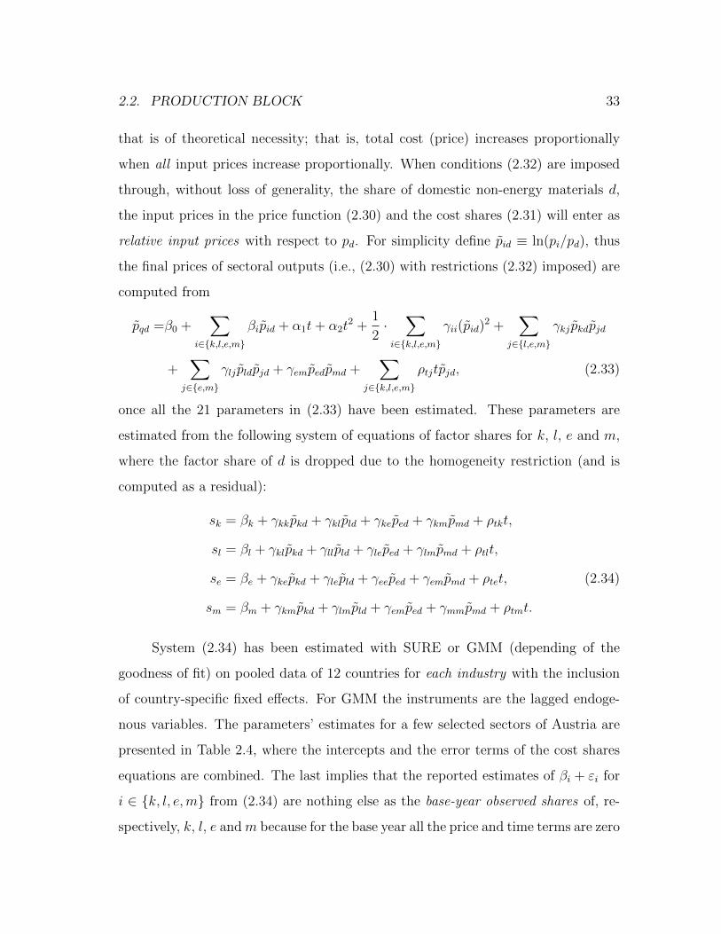
2.2. PRODUCTION BLOCK 33
that is of theoretical necessity; that is, total cost (price) increases proportionally
when all input prices increase proportionally. When conditions (2.32) are imposed
through, without loss of generality, the share of domestic non-energy materials d,
the input prices in the price function (2.30) and the cost shares (2.31) will enter as
relative input prices with respect to pd. For simplicity define pid ≡ ln(pi/pd), thus
the final prices of sectoral outputs (i.e., (2.30) with restrictions (2.32) imposed) are
computed from
pqd =β0 +∑
i∈k,l,e,m
βipid + α1t+ α2t2 +
1
2·∑
i∈k,l,e,m
γii(pid)2 +
∑j∈l,e,m
γkj pkdpjd
+∑
j∈e,m
γlj pldpjd + γempedpmd +∑
j∈k,l,e,m
ρtjtpjd, (2.33)
once all the 21 parameters in (2.33) have been estimated. These parameters are
estimated from the following system of equations of factor shares for k, l, e and m,
where the factor share of d is dropped due to the homogeneity restriction (and is
computed as a residual):
sk = βk + γkkpkd + γklpld + γkeped + γkmpmd + ρtkt,
sl = βl + γklpkd + γllpld + γleped + γlmpmd + ρtlt,
se = βe + γkepkd + γlepld + γeeped + γempmd + ρtet, (2.34)
sm = βm + γkmpkd + γlmpld + γemped + γmmpmd + ρtmt.
System (2.34) has been estimated with SURE or GMM (depending of the
goodness of fit) on pooled data of 12 countries for each industry with the inclusion
of country-specific fixed effects. For GMM the instruments are the lagged endoge-
nous variables. The parameters’ estimates for a few selected sectors of Austria are
presented in Table 2.4, where the intercepts and the error terms of the cost shares
equations are combined. The last implies that the reported estimates of βi + εi for
i ∈ k, l, e,m from (2.34) are nothing else as the base-year observed shares of, re-
spectively, k, l, e andm because for the base year all the price and time terms are zero
34 CHAPTER 2. THEORETICAL FOUNDATIONS OF FIDELIO
(e.g., ped = ln(pe/pd) = ln(1/1) = 0). The base-year observed share of the domestic
non-energy input can be derived as the residual, if needed. For example, for sector
sec01 it is equal to βd = 1−βk−βl−βe−βm = 1−0.366−0.074−0.069−0.093 = 0.398.
The important results derived from the parameters’ estimates of the unit cost
function reported in Table 2.4 are the elasticities of substitution between the factors
of production and the price elasticities of demand. For the translog cost function
the Allen partial elasticities of substitution between inputs i and j are defined as
follows:
σij =c(p) · [∂2c(p)/(∂pi∂pj)]
[∂c(p)/∂pi] · [∂c(p)/∂pj]=
(γij + sisj)/(sisj) if i 6= j,
(γij + s2i − si)/s2
i if i = j,(2.35)
and the price elasticity of demand for factor i with respect to input price j, given
output quantity and all other input prices, are derived from
εij = siσij =
(γij + sisj)/sj if i 6= j,
(γij + s2i − si)/si if i = j.
(2.36)
Observe from (2.35) and (2.36) that although σij = σji for i 6= j, in general,
the price elasticities are not symmetric (i.e., εij 6= εji) because the corresponding
factor shares are different. Note that a positive (resp. negative) value of σij or εij
implies that factors i and j are substitutes (resp. complements), which is important
information for policy objectives. But it should be kept in mind that these are partial
equilibrium concepts and miss various crucial and complex feedback mechanisms
that are captured in models like FIDELIO (for example, all input prices change).
Therefore, the most likely effects on factor demand cannot be directly seen from the
computed price elasticities.
Using (2.36) and Table 2.4 we can compute the price elasticities of demand.
For example, from the last table we see that for the first sector in the base year
the share of its capital is sk = 0.366 and γkk = −0.091. Plugging these values in
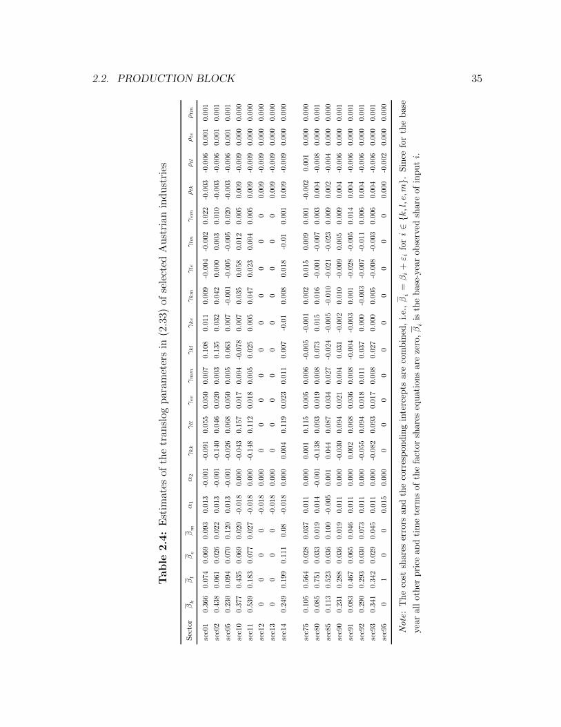
2.2. PRODUCTION BLOCK 35
Table
2.4
:E
stim
ates
ofth
etr
ansl
ogpar
amet
ers
in(2
.33)
ofse
lect
edA
ust
rian
indust
ries
Sec
tor
βk
βl
βe
βm
α1
α2
γkk
γll
γee
γm
mγkl
γke
γkm
γle
γlm
γem
ρtk
ρtl
ρte
ρtm
sec0
10.
366
0.07
40.
069
0.09
30.
013
-0.0
01
-0.0
910.
055
0.0
50
0.0
07
0.108
0.0
11
0.0
09-0
.004
-0.0
02
0.0
22
-0.0
03-0
.006
0.0
01
0.0
01
sec0
20.
438
0.06
10.
026
0.02
20.
013
-0.0
01
-0.1
400.
046
0.0
20
0.0
03
0.135
0.0
32
0.0
420.0
000.
003
0.0
10
-0.0
03
-0.0
060.0
010.
001
sec0
50.
230
0.09
40.
070
0.12
00.
013
-0.0
01
-0.0
260.
068
0.0
50
0.0
05
0.063
0.0
07
-0.0
01
-0.0
05-0
.005
0.0
20
-0.0
03
-0.0
06
0.0
010.0
01
sec1
00.
377
0.43
50.
069
0.02
0-0
.018
0.0
00-0
.043
0.157
0.0
17
0.0
04
-0.0
78
0.0
07
0.0
350.0
580.
012
0.0
050.0
09-0
.009
0.0
000.
000
sec1
10.
539
0.18
30.
077
0.02
7-0
.018
0.0
00-0
.148
0.112
0.0
18
0.0
05
0.025
0.0
05
0.0
470.0
230.
004
0.0
05
0.0
09-0
.009
0.0
000.0
00
sec1
20
00
0-0
.018
0.0
000
00
00
00
00
00.0
09
-0.0
09
0.0
00
0.0
00
sec1
30
00
0-0
.018
0.0
000
00
00
00
00
00.0
09
-0.0
09
0.0
00
0.0
00
sec1
40.
249
0.19
90.
111
0.08
-0.0
180.0
000.0
040.1
190.
023
0.0
11
0.0
07-0
.01
0.0
080.0
18-0
.01
0.0
010.0
09-0
.009
0.0
000.
000
sec7
50.
105
0.56
40.
028
0.03
70.
011
0.0
00
0.0
010.
115
0.0
05
0.0
06-0
.005
-0.0
010.0
020.0
150.
009
0.0
01
-0.0
02
0.0
01
0.0
000.0
00
sec8
00.
085
0.75
10.
033
0.01
90.
014
-0.0
01
-0.1
380.
093
0.0
19
0.0
08
0.073
0.0
15
0.0
16-0
.001
-0.0
07
0.0
03
0.0
04-0
.008
0.000
0.001
sec8
50.
113
0.52
30.
036
0.10
0-0
.005
0.0
010.0
440.0
870.
034
0.0
27
-0.0
24-0
.005
-0.0
10
-0.0
21
-0.0
23
0.0
090.0
02-0
.004
0.0
000.0
00
sec9
00.
231
0.28
80.
036
0.01
90.
011
0.0
00
-0.0
300.0
940.
021
0.0
04
0.0
31-0
.002
0.0
10-0
.009
0.005
0.0
090.0
04-0
.006
0.0
000.
001
sec9
10.
083
0.46
70.
065
0.04
60.
011
0.0
00
0.0
020.
068
0.0
36
0.0
08-0
.004
-0.0
030.0
01-0
.028
-0.0
05
0.0
14
0.0
04-0
.006
0.000
0.001
sec9
20.
290
0.29
30.
030
0.07
30.
011
0.0
00
-0.0
550.0
940.
018
0.0
11
0.0
370.
000
-0.0
03
-0.0
07-0
.011
0.0
06
0.0
04-0
.006
0.000
0.001
sec9
30.
341
0.34
20.
029
0.04
50.
011
0.0
00
-0.0
820.0
930.
017
0.0
08
0.0
270.
000
0.005
-0.0
08
-0.0
030.0
060.0
04-0
.006
0.0
000.
001
sec9
50
10
00.
015
0.0
000
00
00
00
00
00.
000
-0.0
02
0.000
0.0
00
Note
:T
he
cost
shar
eser
rors
and
the
corr
esp
on
din
gin
terc
epts
are
com
bin
ed,
i.e.
,βi
=βi
+ε i
fori∈k,l,e,m.
Sin
cefo
rth
eb
ase
year
all
oth
erp
rice
and
tim
ete
rms
ofth
efa
ctor
share
seq
uati
on
sare
zero
,βi
isth
eb
ase
-yea
rob
serv
edsh
are
of
inpu
ti.
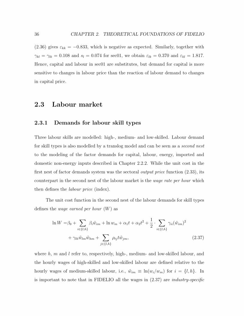
36 CHAPTER 2. THEORETICAL FOUNDATIONS OF FIDELIO
(2.36) gives εkk = −0.833, which is negative as expected. Similarly, together with
γkl = γlk = 0.108 and sl = 0.074 for sec01, we obtain εlk = 0.370 and εkl = 1.817.
Hence, capital and labour in sec01 are substitutes, but demand for capital is more
sensitive to changes in labour price than the reaction of labour demand to changes
in capital price.
2.3 Labour market
2.3.1 Demands for labour skill types
Three labour skills are modelled: high-, medium- and low-skilled. Labour demand
for skill types is also modelled by a translog model and can be seen as a second nest
to the modeling of the factor demands for capital, labour, energy, imported and
domestic non-energy inputs described in Chapter 2.2.2. While the unit cost in the
first nest of factor demands system was the sectoral output price function (2.33), its
counterpart in the second nest of the labour market is the wage rate per hour which
then defines the labour price (index).
The unit cost function in the second nest of the labour demands for skill types
defines the wage earned per hour (W ) as
lnW =β0 +∑i∈l,h
βiwim + lnwm + α1t+ α2t2 +
1
2·∑i∈l,h
γii(wim)2
+ γlhwlmwhm +∑j∈l,h
ρtjtwjm, (2.37)
where h, m and l refer to, respectively, high-, medium- and low-skilled labour, and
the hourly wages of high-skilled and low-skilled labour are defined relative to the
hourly wages of medium-skilled labour, i.e., wim ≡ ln(wi/wm) for i = l, h. In
is important to note that in FIDELIO all the wages in (2.37) are industry-specific
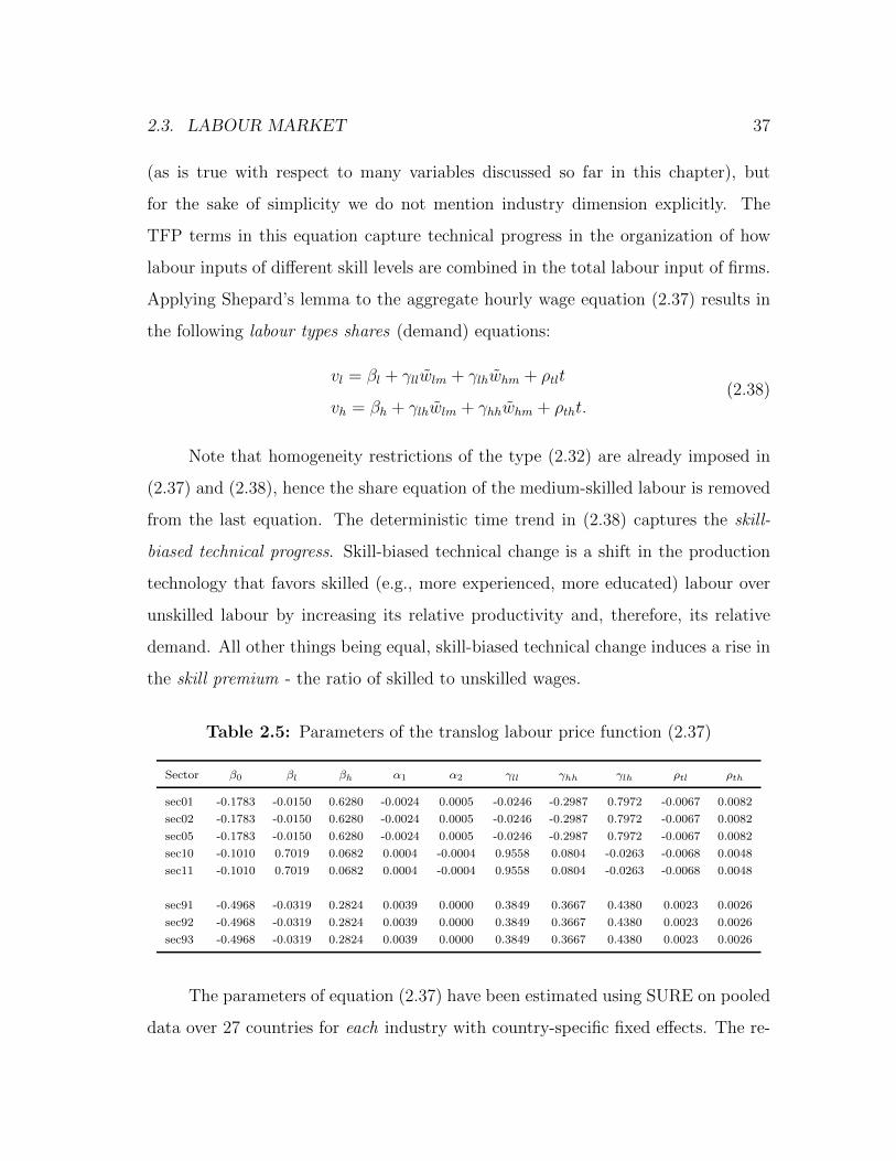
2.3. LABOUR MARKET 37
(as is true with respect to many variables discussed so far in this chapter), but
for the sake of simplicity we do not mention industry dimension explicitly. The
TFP terms in this equation capture technical progress in the organization of how
labour inputs of different skill levels are combined in the total labour input of firms.
Applying Shepard’s lemma to the aggregate hourly wage equation (2.37) results in
the following labour types shares (demand) equations:
vl = βl + γllwlm + γlhwhm + ρtlt
vh = βh + γlhwlm + γhhwhm + ρtht.(2.38)
Note that homogeneity restrictions of the type (2.32) are already imposed in
(2.37) and (2.38), hence the share equation of the medium-skilled labour is removed
from the last equation. The deterministic time trend in (2.38) captures the skill-
biased technical progress. Skill-biased technical change is a shift in the production
technology that favors skilled (e.g., more experienced, more educated) labour over
unskilled labour by increasing its relative productivity and, therefore, its relative
demand. All other things being equal, skill-biased technical change induces a rise in
the skill premium - the ratio of skilled to unskilled wages.
Table 2.5: Parameters of the translog labour price function (2.37)
Sector β0 βl βh α1 α2 γll γhh γlh ρtl ρth
sec01 -0.1783 -0.0150 0.6280 -0.0024 0.0005 -0.0246 -0.2987 0.7972 -0.0067 0.0082
sec02 -0.1783 -0.0150 0.6280 -0.0024 0.0005 -0.0246 -0.2987 0.7972 -0.0067 0.0082
sec05 -0.1783 -0.0150 0.6280 -0.0024 0.0005 -0.0246 -0.2987 0.7972 -0.0067 0.0082
sec10 -0.1010 0.7019 0.0682 0.0004 -0.0004 0.9558 0.0804 -0.0263 -0.0068 0.0048
sec11 -0.1010 0.7019 0.0682 0.0004 -0.0004 0.9558 0.0804 -0.0263 -0.0068 0.0048
sec91 -0.4968 -0.0319 0.2824 0.0039 0.0000 0.3849 0.3667 0.4380 0.0023 0.0026
sec92 -0.4968 -0.0319 0.2824 0.0039 0.0000 0.3849 0.3667 0.4380 0.0023 0.0026
sec93 -0.4968 -0.0319 0.2824 0.0039 0.0000 0.3849 0.3667 0.4380 0.0023 0.0026
The parameters of equation (2.37) have been estimated using SURE on pooled
data over 27 countries for each industry with country-specific fixed effects. The re-
38 CHAPTER 2. THEORETICAL FOUNDATIONS OF FIDELIO
sults are reported in Table 2.5 for selected sectors. In case the estimated parameters
did not yield negative own price elasticities, these elasticities have been set equal
to zero and not restricted. The philosophy behind such estimation strategy is that
substitution between different segments of the labour market is a much stronger
“null hypothesis” than between the first nest production factors (i.e., between cap-
ital, labour, energy inputs, domestic and imported non-energy inputs) and should
be assumed not to exist, if it cannot be proven with the data.
2.3.2 Wage curves
Following a meta analysis of Folmer (2009), the sectoral hourly wages by skill type,
i.e., wi’s in (2.37) and (2.38), are derived from the so-called wage curves (or func-
tions). The wage curve describes the responsiveness of individual real wages to the
changing local market conditions. In their pathbreaking work, Blanchflower and
Oswald (1994) found that there is a stable relationship in the form of downward-
sloping convex curve between local unemployment and the level of wages, which
establishes the so-called empirical “law” of economics they characterized as “the
wage curve”. They also argue that for most purposes, the wage curve relation is
well approximated by a simple log-linear function.
Based on the detailed review of some hundred articles, books and working
papers, Folmer (2009) gathers and computes 1004 elasticities of pay in disaggregated
(industry of labour market segment) macro equations. In FIDELIO three wage
elasticities reported in the mentioned study are used. These are related to labour
productivity (Q/L), consumer price (PC) and unemployment rate by skill level (UR).
That is, the first two explanatory variables are invariant with respect to the labour
skill type, while the last is labour skill-specific variable. The log-linear versions of
the (long-run) wage equations for labour skill type i = l,m, h that need to be
2.3. LABOUR MARKET 39
used in the empirical applications are given by
lnwi = constanti + τ1 ln(Q/L) + τ2 ln(PC) + τi ln(URi). (2.39)
Again we note that for simplicity of exposition (and to be consistent with previous
section notations) we dropped the industry dimension from wi and the constant
term constanti in (2.40), and country dimension for all the mentioned variables. The
constant term accounts for the unexplained industry component in determination
of wages by skill level.
In FIDELIO, however, wage curves determine yearly wages per employee by
skill level, similar to Folmer (2009) meta analysis, and not hourly wages as given in
(2.39). That is, we use instead
lnwemi = constanti + τ1 ln(Q/L) + τ2 ln(PC) + τi ln(URi), (2.40)
where wemi denotes wage per employee of labour skill type i = l,m, h. The
reasons for using wemi instead of wi in the wage curve are mainly two-fold:
1. The wage elasticities in (2.39) and (2.40) “are similar, given that extra remu-
nerations are proportional to the hourly wage rate and that changes in total
number of hours worked are taken into account in the yearly wage equation”
(Folmer 2009, p. 54).
2. By dealing with costs by employee for labour demand, we take into account
certain short-term fixed characteristics of labour cost and the input of labour
cannot adjust immediately. Therefore, changing hours per employee becomes
a way of adjusting labour (like the German “Kurzarbeit” during the recent
recession) or a policy variable.3
3This design of the wage rate is therefore also chosen with the perspective of a possible simulationof shortening working time. If we do so in FIDELIO, we would on the one hand (ceteris paribus)have the pure calculation effect of distributing given quantity of labour across more employees andon the other hand also the effect of a correspondingly higher wage costs, so that demand for labourwill adjust. This latter effect can be seen in analogy to the “rebound effect” of energy efficiencyincreases.
40 CHAPTER 2. THEORETICAL FOUNDATIONS OF FIDELIO
Thus, the hourly wage by skill type wi is then simply derived by dividing the wages
per employee wemi by the so-called working time (exogenous) variable which is
nothing else as the total hours worked per employee (and varies by sector and region).
The estimates of the required parameters in (2.40) are the benchmark values
of the corresponding long-term (average) elasticities reported in Folmer (2009, pp.
38-39). The information on the reported short-term elasticities values have been
ignored because the differences between the two are rather small. Folker makes the
following breakdown of the countries:
- The Netherlands
- Anglo-Saxon countries: Australia, Canada, New Zealand, UK, USA
- Nordic countries: Denmark, Finland, Norway, Sweden
- All other countries
The values of τ1, τ2 and τ3 = τl = τm = τh in (2.40) are assumed to be the same
for all labour skill types and the corresponding estimates reported in Folmer (2009)
are presented in Table 2.6. From the table we observe that whenever unemployment
increases, wages in all regions/coutnries decrease. The corresponding elasticity is
lowest for Anlgo Saxon countries (-4.3%) and much higher (in absolute terms) for the
remaining countries (from -7.9% to -9.0%). This might be explained by the fact that
the Anglo Saxon countries have less generous welfare state than the others. “The
lower the real unemployment benefits, the stronger the incentive to look for a new
job in case of unemployment and the lower the reservation wage. So an additional
rise in unemployment may have lesser impact on search intensity and wages than in
more generous welfare states like those of Nordic countries and The Netherlands”
(Folmer, 2009, p. 40).
The wage equations by skill and industry in each region (group of regions)
comprise an industry component that cannot be explained by differences in the skill

2.3. LABOUR MARKET 41
Table 2.6: Elasticities of the wage curves in (2.40)
Regions τ1 τ2 τ3
AUT/BEL/LUX/NLD 0.832 0.584 -0.080
Anglo Saxon 0.921 0.580 -0.043
Nordic countries 0.921 0.520 -0.090
Other countries 0.921 0.580 -0.079
Source: Folmer (2009, pp. 38-39).
structure and labour productivity of industries. The literature on inter-industry
wage differentials in Europe (Du Caju et al., 2010) shows the significant magnitude
of this differential and reveals the role of industry specific factors as rent-sharing
mechanisms. Though from an academic point of view the unresolved puzzles of
inter-industry wage differentials might be seen as disappointing, the integration of
this component in an inter-industry model like FIDELIO adds an important degree
of differentiation.
It is important to note what the wage curve does not represent. First, the
wage curve is not the famous Phillips curve traditionally taught in macroeconomics
courses, named after Alban Phillips (see Phillips, 1958). This is because in wage
curve contemporaneous unemployment rate determines the level of wages (adjusted
for permanent market-specific differentials), while Phillips curve postulates the ex-
istence of negative relation (or short-term tradeoff) between the contemporaneous
unemployment rate and the rate of change of wages. Second, Blanchflower and
Oswald (1994) argue that their wage curve is not a labour supply function. This
could be a plausible interpretation because as “short run changes in employment
and unemployment are approximately mirror images, a finding that wages rise with
contemporaneous reductions in unemployment may simply reflect movements along
an upward-sloping labor supply function” (Card, 1995, p. 795). This interpretation
42 CHAPTER 2. THEORETICAL FOUNDATIONS OF FIDELIO
is rejected by Blanchflower and Oswald empirical results which strongly support the
view that it is local unemployment, and not local employment or the size of the
local labour force, that effects wages. Since most economists think of labour supply
curve in terms of total quantity of labour supplied as a function of wages, these
findings seem, indeed, to be inconsistent with the second mentioned interpretation.
Rejecting both interpretations, Blanchflower and Oswald (1994) argue that their
findings represents something new, which thus they call “the wage curve”.
In his excellent review of Blanchflower and Oswald’s work, Card (1995) con-
cluded that “the existence of a wage curve relation is an important addition to our
knowledge about the modern labor market. ... Many readers will be stimulated by
the conclusion that the wage curve is “something new”: a surrogate supply function
that can be combined with a simple demand curve to yield interesting models of the
labor market; a challenge to orthodox theories of supply and demand” (p. 798). It is
namely in this context that the wage curve is used in FIDELIO, i.e., the “surrogate
supply functions” (2.40) together with the derived labour demands (2.38) determine
the “equilibrium” quantities of labour skill types.
Chapter 3
Derivation of the base-year data
In this chapter we discuss the relationships among and the derivations of all the
necessary variables, mainly for the base year. All the major data sources, which
make the core dataset of FIDELIO, are listed in Chapter 5. In the Appendix we
also give the definitions all the variables used in FIDELIO, which further contributes
to the easier processing of the material presented in this and the next chapters.
3.1 Basic price data
The base-year use table at basic prices is, by definition, derived from the use table
at purchasers’ prices adjusted for the trade and transport margins and taxes less
subsidies, i.e.,
USEbp(r, g, u) = USEpp(r, g, u)−MRG(r, g, u)− TXS(r, g, u). (3.1)
The values of gross outputs (i.e., gross outputs in nominal terms) by region and sector
are obtained from the corresponding make matrix by summing over all goods:1
1Note that Q does not mean “quantities in physical terms” as, for example, in CGE modelling,but denotes “quantities in nominal terms”. We could have used VQ instead of Q to indicate this
43
44 CHAPTER 3. DERIVATION OF THE BASE-YEAR DATA
Q(r, s) =∑
g
MAKE(r, g, s). (3.2)
Total value added at basic prices can be derived as a residual, i.e.,
VA(r, s) = Q(r, s)−∑
g
USEpp(r, g, s). (3.3)
3.2 Shares and structure matrices
In FIDELIO sectoral outputs are computed from the demands for domestically pro-
duced goods based on the assumption of constant market shares. The corresponding
market share matrix shows the proportions (shares) of industries’ outputs in the pro-
duction of each good, and is defined as
MKSH(r, g, s) = MAKE(r, g, s)/∑
s
MAKE(r, g, s). (3.4)
Hence, by definition, for each good and each region the sum of the market shares over
all sectors equals unity. Equation (3.4) is defined only for goods that are produced
domestically. The entries corresponding to zero domestic outputs of the market
share matrix are set to zero. Without further mentioning, such a rule with zero
denominators is applied to all the relevant cases (formulas) discussed below.
The total intermediate use at purchasers’ prices for each region and each user
(which refers to sectors and final demand categories) is obtained as
S(r, u) =∑
g
USEpp(r, g, u). (3.5)
Note from (3.5) that S(r,s) represents base-year demand for total intermediate inputs
by sector s located in region r.
fact, but the last adapted notation is simpler.
3.2. SHARES AND STRUCTURE MATRICES 45
Using (3.2) and (3.5), the total intermediate inputs shares are obtained from
S Q(r, s) = S(r, s)/Q(r, s). (3.6)
FIDELIO’s production block distinguishes between energy (E) and non-energy
(N) intermediate inputs. The total energy inputs include domestic and imported
intermediate inputs of five energy goods:
E(r, s) =∑ge
USEpp(r, ge, s), (3.7)
where ge (energy goods identifier) refers to products “Coal and lignite; peat”, “Crude
petroleum and natural gas”, “Uranium and thorium ores”, “Coke, refined petroleum
production and nuclear fuels”, and “Electrical energy, gas, steam and hot water”.
Similarly, total non-energy inputs is the aggregate of domestic and imported
inputs of all non-energy products, i.e.,
N(r, s) =∑gne
USEpp(r, gne, s). (3.8)
The energy inputs shares in gross outputs by sectors and regions are then
defined as
E Q(r, s) = E(r, s)/Q(r, s). (3.9)
Consequently, the shares of non-energy inputs can be obtained as residuals, i.e.,
N Q(r, s) = S Q(r, s)− E Q(r, s). (3.10)
To distinguish between domestic and imported non-energy intermediate inputs,
we need the import shares matrix which shows the proportion of total imported
products from the corresponding basic price uses, i.e.,
MSH(r, g, u) = MUSE(r, g, u)/USEbp(r, g, u). (3.11)
46 CHAPTER 3. DERIVATION OF THE BASE-YEAR DATA
The matrices of imported non-energy inputs (M) and domestic non-energy inputs
(D) are derived using the import shares matrix (3.11) as follows:
M(r, s) =∑gne
USEpp(r, gne, s) ·MSH(r, gne, s), (3.12)
D(r, s) =∑gne
USEpp(r, gne, s) ·[1−MSH(r, gne, s)
]. (3.13)
Note that, by definition, N(r, s) = D(r, s) + M(r, s). The base-year shares of M and
D in gross outputs are, respectively,
M Q(r, s) = M(r, s)/Q(r, s), (3.14)
D Q(r, s) = D(r, s)/Q(r, s). (3.15)
The shares of labour compensation, which includes wages and social security
contributions, in gross output are obtained from the base-year value added compo-
nents matrix, VAC, as
L Q(r, s) =[VAC(r,wage, s) + VAC(r, soc.sec.cont, s)
]/Q(r, s). (3.16)
The sum of all value added components without labour compensation is defined as
capital compensation or cash flow. That is, the value of capital inputs is the sum
of production taxes net of production subsidies, depreciation and operating profits.
Given the input-output expenditure-side accounting identity, the share of capital in
gross output can be derived as the residual:
K Q(r, s) = 1− S Q(r, s)− L Q(r, s). (3.17)
The shares of employers’ social security contributions in total labour compensation
are
SSC L(r, s) =VAC(r, soc.sec.cont, s)
VAC(r,wage, s) + VAC(r, soc.sec.cont, s). (3.18)
The shares of production taxes in gross outputs is obtained from
TXP Q(r, s) = VAC(r, prdn.tax, s)/Q(r, s). (3.19)
3.2. SHARES AND STRUCTURE MATRICES 47
Similarly, the base-year shares of production subsidies and of depreciation in gross
outputs are given, respectively, by
SBP Q(r, s) = VAC(r, prdn.sub, s)/Q(r, s), (3.20)
DPR Q(r, s) = VAC(r, depr, s)/Q(r, s). (3.21)
The shares of investment goods in gross outputs that could be used in deriving
investment demands are obtained as
I Q(r, s) =∑
g
INVpp(r, g, s)/Q(r, s). (3.22)
The option that is used in FIDELIO for deriving investment demands consists of
linking investments to sectoral capital stocks using the investment-capital stock ra-
tios from the base-year data, i.e.,
I K(r, s) =∑
g
INVpp(r, g, s)/KS(r, s), (3.23)
where KS(r,s) is the capital stock of sector s in region r.
The product use structure matrix of a region shows for each user the purchasers’
price values of the uses of imported and domestic goods per total its (intermediate
or final) used goods, hence is defined as
USTR(r, g, u) = USEpp(r, g, u)/∑
g
USEpp(r, g, u). (3.24)
Similar structure matrices are defined for energy and non-energy inputs separately.
Using (3.7), the matrix of product structure of energy inputs is obtained from
ESTR(r, g, s) =
USEpp(r, g, s)/E(r, s) if g = ge,
0 if g = gne.(3.25)
Similarly, using total non-energy intermediate inputs (3.8) and the use table at
purchasers’ prices, the product structure of non-energy inputs is derived as
NSTR(r, g, s) =
USEpp(r, g, s)/N(r, s) if g = gne,
0 if g = ge.(3.26)
48 CHAPTER 3. DERIVATION OF THE BASE-YEAR DATA
Using (3.11) and (3.12), the product structure of imported non-energy inputs
is obtained from
MSTR(r, g, s) =
[USEpp(r, g, s) ·MSH(r, g, s)
]/M(r, s) if g = gne,
0 if g = ge.(3.27)
Similarly, using the import share matrix (3.11) and the matrix of domestic non-
energy intermediate inputs (3.13), the product structure of domestic non-energy in-
puts is derived as follows:
DSTR(r, g, s) =
[USEpp(r, g, s) · (1−MSH(r, g, s))
]/D(r, s) if g = gne,
0 if g = ge.(3.28)
Note that for each region r and each sector s the sum over all goods of the structure
matrices ESTR, NSTR, MSTR and DSTR is unity, by construction. This fact is
used later in the allocation of aggregate inputs of energy, imported and domestic
non-energy materials over all products in order to compute the sectoral demands for
intermediate goods at purchasers’ prices.
The product structure of investments (at purchasers’ prices) is defined as
ISTR(r, g, s) = INVpp(r, g, s)/∑
g
INVpp(r, g, s). (3.29)
For each region and each user, the product tax net of subsidy rate is given by
TXSR(r, g, u) = TXS(r, g, u)/USEpp(r, g, u). (3.30)
The rates of total margins (trade and transport) paid on non-margin goods are ob-
tained from
MGRpaid(r, g, u)
=
MRG(r, g, u)/[USEpp(r, g, u)− TXS(r, g, u)
]if g = gnm,
0 ifg = gm.(3.31)

3.2. SHARES AND STRUCTURE MATRICES 49
The share of total margins received by a margin good (i.e., share of a margin good
in total margins) is computed from
MGSrec.(r, g, u) =
MRG(r, g, u)/∑
gm1MRG(r, gm1, u) if g = gm,
0 if g = gnm.(3.32)
For simplicity of exposition, let us define for each good and each user, the
shares of total margins in the corresponding uses at basic prices plus margins as
follows:
MG MGU(r, g, u) ≡ MRG(r, g, u)/ [USEbp(r, g, u) + MRG(r, g, u)] . (3.33)
Then using the margin shares of margin goods (3.32), the matrix of price structure
of domestically produced goods can be defined as
PSTR(r, g, u, g1)
=
1 if g = g1 = gm,
1−MG MGU(r, g, u) if g = g1 = gnm,
MG MGU(r, g, u) ·MGSrec.(r, g1, u) if gn = g 6= g1 = gm,
0 otherwise.
(3.34)
Note that∑
g1PSTR(r, g, u, g1) = 1 for each region r, each good g and each user u.
For each margin good g = gm, PSTR has only one positive element always equal
to unity corresponding to the same margin good. But, for each non-margin good
g = gn in PSTR(r, g, u, g1) we have the following positive elements: (a) position
(gn, gn) indicates the proportion of gn’s use at basic prices in its use at basic prices
plus margins, and (b) positions (gn, gm’s) indicate the proportion of gn’s margins
in its use at basic prices plus margins that is distributed over all margin goods gm’s
according to their shares in generating total margins. This price structure matrix
along with information on the rates of products’ net taxes (3.30) will be used in the
model simulations to translate basic prices of domestic goods g1 into the purchasers’
prices of domestically produced goods g.

50 CHAPTER 3. DERIVATION OF THE BASE-YEAR DATA
The following regional shares are based on the data on financial balances of
households (FBHH). Taxes on households will be determined from income tax rate
that is defined as
Tx Inc(r) =FBHH(r, taxes)
FBHH(r,wage) + FBHH(r, oper.surp)− FBHH(r, soc.con.gov).
(3.35)
Note that FBHH data are obtained from National Accounts (NA) sources and not
from the supply and use tables (SUTs). As such the SUTs-based data need to be
re-scaled so as to match those of the NA data. For this purpose, simple scale ratios
are used. These are the NA to input-output (IO, or SUT) ratios of wages, social
security contributions (Sscn) and operating surplus (Opsp):
Wagena.io(r) =FBHH(r,wage)∑
s [VAC(r,wage, s) + VAC(r, soc.sec.cont, s)], (3.36)
Sscnna.io(r) =FBHH(r, soc.con.gov)∑s VAC(r, soc.sec.cont, s)
, (3.37)
Opspna.io(r) =FBHH(r, oper.surp)∑s VAC(r, oper.surp, s)
. (3.38)
3.3 Trade matrix construction
There are two options for taking into account the costs for third countries to transit
non-service goods from one region to another. A simple and ad hoc option is to use
the data for transit costs powers2 that are computed as follows
TNCS(r, r1, g) = 1 + 0.06 · Distance(r, r1)
MaxDist, (3.39)
where MaxDist is the maximum distance between a pair of regions included in the
model, except for the rest of the world (RoW). The number 0.06 in (3.39) simply
means that the transit costs are assumed not to be larger than 6% of the value
2Power of a variable is defined as one plus the rate of change (or interest) of that variable.
3.3. TRADE MATRIX CONSTRUCTION 51
of any transaction between countries. Transit costs of all non-service goods to the
RoW are set to 1.08 for all regions. For service goods transit costs are zero, hence
the corresponding TNCS elements are set to unity.
A more realistic estimates of the international transit costs, that are also used
in FIDELIO-1, are derived by Streicher and Stehrer (2012). In contrast to (3.39), for
each pair of the exporting and importing countries, these estimates also vary across
(non-service) goods. We do not discuss the details of these transit costs derivation
here and refer the interested reader to the mentioned study.
Let us denote the WIOD trade matrix by TRDwiod(r, r1, g, u), where the first
region r is the importing (destination) region, while the second region r1 is the
exporting (source) region. Further, the total EU-imports of each region r given in
MUSEeu(r, g, u) are expressed in national currencies. The initial trade matrix at CIF
prices expressed in euros is obtained as
TRDcif(r, r1, g, u) =
0 if r = r1,
MUSEeu(r,g,u)Xrate(r)
· TRDwiod(r,r1,g,u)∑r2 6=r TRDwiod(r,r2,g,u)
if r 6= r1
(3.40)
where r is the destination region and r1 is the source region. In (3.40) the WIOD’s
trade matrix TRDwiod is used for the distribution of imports to the trading partners
and is not used itself because the product import shares of all sectors in this matrix
are identical, while a more realistic picture of the imports is given in the use tables;
hence both data are used in (3.40).
The matrix of trade in FOB prices is then obtained by taking into account the
corresponding transit costs, TNCS:
TRD fob(r, r1, g, u) = TRDcif(r, r1, g, u)/TNCS(r, r1, g). (3.41)
However, then one needs to ensure that in the derived trade matrices (3.40) and
(3.41): (i) all imports are accounted for (i.e., the sum over all trading partners’
52 CHAPTER 3. DERIVATION OF THE BASE-YEAR DATA
shares equals one) and (ii) on the exporting partners’ side, the sum of CIF-imports
by the trading partners corrected for international trade and transport margins has
to equal the export vector valued at FOB (here it is the exports within the EU area,
exp eu). To ensure these two conditions, exports to and imports from the RoW are
taken as residuals. The analytical representation of this procedure is given by the
following steps:
start loop
TRDcif(r, r1, g, u) =MUSEeu(r, g, u)
Xrate(r)· TRDcif(r, r1, g, u)∑
r2TRDcif(r, r2, g, u)
,
Re-compute TRDfob(r, r1, g, u) using Equation (3.41),
TRDfob(r, r1, g, u) = TRDfob(r, r1, g, u) ·min
[1,
USEpp(r1, g, exp eu)/Xrate(r1)∑r2,u1
TRDfob(r2, r1, g, u1)
],
TRDcif(r, r1, g, u) = TRDfob(r, r1, g, u) · TNCS(r, r1, g)
end loop
until the trade matrices at CIF prices TRDcif(r, r1, g, u) from the first and final steps
of a particular loop (described above) converge to each other. Then we obtain again
TRDfob using (3.41). Adding the RoW as additional region to the trade matrices,
the imports of an EU-region r from the RoW is computed as the difference between
the total imports and the EU-imports of region r:
TRDcif(r, row, g, u) =MUSE(r, g, u)
Xrate(r)−∑
r1
TRDcif(r, r1, g, u). (3.42)
Then the new TRDfob is obtained by plugging (3.42) in (3.41) which now also in-
cludes the RoW region. Using this new TRDfob matrix, total exports of an EU-region
r to the RoW is again obtained as a residual (‘exp’ stands for total exports):
TRDfob(row, r, g, exp) =USEpp(r, g, exp)
Xrate(r)−∑r1,u
TRDfob(r1, r, g, u). (3.43)
3.4. COICOP-CPA BRIDGE MATRICES 53
From (3.43) we ultimately find the vector of exports to the RoW in national cur-
rencies, i.e., exports that are not accounted for by trade within the model regions
(which will be taken as exogenous in the baseline simulation):
EXProw(r, g) = TRDfob(row, r, g, exp) · Xrate(r). (3.44)
For region r its trading partners’ import shares in its total imports by each
user and each good is defined as
TMSH(r, rt, g, u) =TRDcif(r, rt, g, u)
MUSE(r, g, u)/Xrate(r). (3.45)
Note that the first step of the trade matrix adjustment procedure outlined above
guarantees that∑
rt TMSH(r, rt, g, u) = 1 for all r, g and u. However because of the
problem of memory, the number of users needs to be reduced in the trade matrix.
Therefore, the reduced matrix of trading partners’ import shares is defined only for
seven trade users (utr), which are all intermediate users as one sector (st) and six
final demanders (f). Hence,
TMSHred(r, rt, g, utr) =
TMSH(r, rt, g, f) if utr = f,∑s TMSH(r, rt, g, s) if utr = st.
(3.46)
3.4 COICOP-CPA bridge matrices
The base-year and the required lagged data on private consumption of COICOP
commodities C(r,c,t) are derived from the national accounts information. For FI-
DELIO purposes, the 47 components of the individual consumption expenditure
of households of the COICOP classification at 3-digit level are aggregated to 17
commodities, from which 12 are nondurables and 5 are durable goods.
As an illustration, Table 3.1 shows the details of these commodities in the
example of Austria for the years of 2000 to 2005. In addition to the durables and
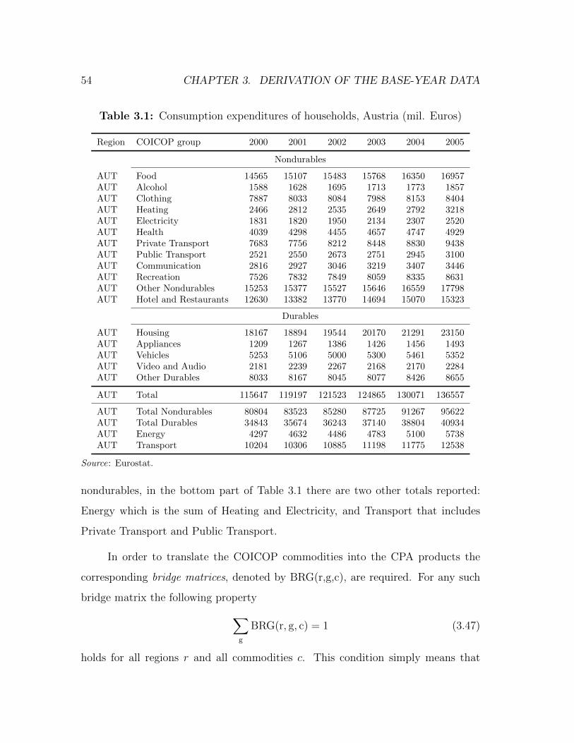
54 CHAPTER 3. DERIVATION OF THE BASE-YEAR DATA
Table 3.1: Consumption expenditures of households, Austria (mil. Euros)
Region COICOP group 2000 2001 2002 2003 2004 2005
Nondurables
AUT Food 14565 15107 15483 15768 16350 16957AUT Alcohol 1588 1628 1695 1713 1773 1857AUT Clothing 7887 8033 8084 7988 8153 8404AUT Heating 2466 2812 2535 2649 2792 3218AUT Electricity 1831 1820 1950 2134 2307 2520AUT Health 4039 4298 4455 4657 4747 4929AUT Private Transport 7683 7756 8212 8448 8830 9438AUT Public Transport 2521 2550 2673 2751 2945 3100AUT Communication 2816 2927 3046 3219 3407 3446AUT Recreation 7526 7832 7849 8059 8335 8631AUT Other Nondurables 15253 15377 15527 15646 16559 17798AUT Hotel and Restaurants 12630 13382 13770 14694 15070 15323
Durables
AUT Housing 18167 18894 19544 20170 21291 23150AUT Appliances 1209 1267 1386 1426 1456 1493AUT Vehicles 5253 5106 5000 5300 5461 5352AUT Video and Audio 2181 2239 2267 2168 2170 2284AUT Other Durables 8033 8167 8045 8077 8426 8655
AUT Total 115647 119197 121523 124865 130071 136557
AUT Total Nondurables 80804 83523 85280 87725 91267 95622AUT Total Durables 34843 35674 36243 37140 38804 40934AUT Energy 4297 4632 4486 4783 5100 5738AUT Transport 10204 10306 10885 11198 11775 12538
Source: Eurostat.
nondurables, in the bottom part of Table 3.1 there are two other totals reported:
Energy which is the sum of Heating and Electricity, and Transport that includes
Private Transport and Public Transport.
In order to translate the COICOP commodities into the CPA products the
corresponding bridge matrices, denoted by BRG(r,g,c), are required. For any such
bridge matrix the following property∑g
BRG(r, g, c) = 1 (3.47)
holds for all regions r and all commodities c. This condition simply means that
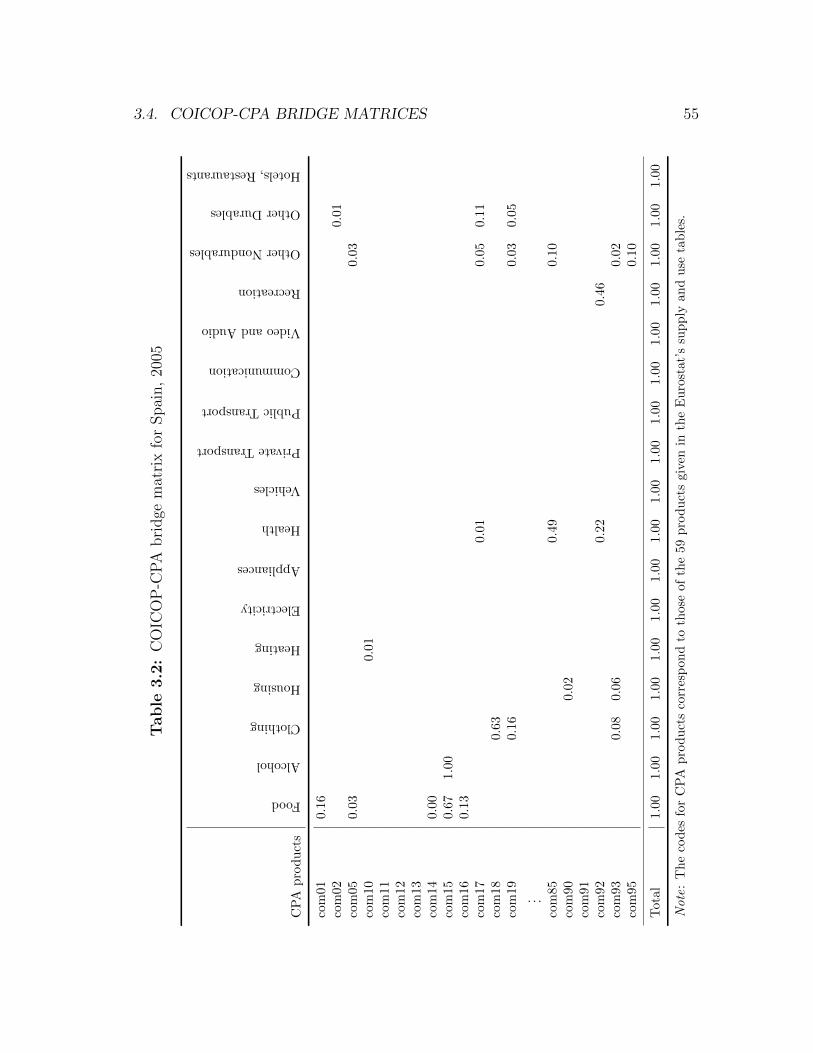
3.4. COICOP-CPA BRIDGE MATRICES 55
Table
3.2
:C
OIC
OP
-CP
Abri
dge
mat
rix
for
Spai
n,
2005
CP
Ap
rod
uct
s
Food
Alcohol
Clothing
Housing
Heating
Electricity
Appliances
Health
Vehicles
PrivateTransport
PublicTransport
Communication
VideoandAudio
Recreation
OtherNondurables
OtherDurables
Hotels,Restaurants
com
010.
16co
m02
0.0
1co
m05
0.03
0.0
3co
m10
0.0
1co
m11
com
12co
m13
com
140.
00co
m15
0.67
1.00
com
160.
13co
m17
0.0
10.0
50.1
1co
m18
0.63
com
190.
160.0
30.0
5. . .
com
850.4
90.1
0co
m90
0.02
com
91co
m92
0.2
20.4
6co
m93
0.08
0.06
0.0
2co
m95
0.1
0
Tot
al1.
001.
001.
001.
001.0
01.0
01.0
01.0
01.0
01.0
01.0
01.0
01.0
01.0
01.0
01.0
01.0
0
Note
:T
he
cod
esfo
rC
PA
pro
du
cts
corr
esp
on
dto
those
of
the
59
pro
du
cts
giv
enin
the
Eu
rost
at’
ssu
pply
an
du
seta
ble
s.
56 CHAPTER 3. DERIVATION OF THE BASE-YEAR DATA
each of the COICOP commodity should be distributed over all the relevant CPA
products.
As an example in Table 3.2 we present the (incomplete over the CPA products
dimension) bridge matrix of Spain for 2005. The first column of this bridge matrix
shows that the COICOP commodity “Food” is distributed according to the given
proportions over five CPA products, which are “Products of agriculture, hunting
and related services” (code: com01), “Fish and fishing products” (com05), “Other
mining and quarrying products” (com14), “Food products and beverages” (com15)
and “Tobacco products” (com16). Similarly, commodity “Alcohol” is allocated en-
tirely to “Food products and beverages” (com15) as the corresponding element is
unity, i.e., BRG(ESP, com15,Alcohol) = 1. Therefore, the column coefficients of
each COICOP commodity of the bridge matrix can be also interpreted as house-
holds’ consumption technology according to which CPA products are used as inputs
by individuals to “produce” (a bundle of) commodities for their own needs. This
notion was first explored by Lancaster (1966). For recent discussion of this concept
see e.g., Mongelli et al. (2010).
3.5 Consumption block residuals
In the consumption block of FIDELIO durable commodities are modelled as stocks,
from which then the corresponding flows are obtained. For the explicit distinc-
tion of this fact, we denote region r’s stock and flow of the durable commodity
cd, respectively, as CS(r,cd) and C(r,cd). The estimates of the parameters of the
nondurable and durable policy functions in their ADL(2,2,2) specifications (2.8)
and (2.9) are included in the consumption block coefficient matrices Φr,cdCS,coefficient
and Φr,ctnC,coefficient, respectively. That is, (Φr,ctn
C,1 ,Φr,ctnC,2 , . . . ,Φ
r,ctnC,8 )′ = (α1, α2, . . . , α8)′
and (Φr,cdCS,1,Φ
r,cdCS,2, . . . ,Φ
r,cdCS,8)′ = (β1, β2, . . . , β8)′. The corresponding values are all

3.5. CONSUMPTION BLOCK RESIDUALS 57
reported in Table 2.1. Using durable consumption demand equation (2.9), the cor-
responding base-year residuals are derived as
RCS(r, cd) =ln CS(r, cd)
−
Φr,cdCS,1 · ln CS1(r, cd) + Φr,cd
CS,2 · ln CS2(r, cd)
+Φr,cdCS,3 · ln [Tht(r) + PCS(r, cd)]
+Φr,cdCS,4 · ln [Tht1(r) + PCS1(r, cd)] (3.48)
+Φr,cdCS,5 · ln [Tht2(r) + PCS2(r, cd)]
+Φr,cdCS,6 · ln Zz(r) + Φr,cd
CS,7 · ln Zz1(r) + Φr,cdCS,8 · ln Zz2(r)
,
where PCS(r,cd) are the observed prices of durable commodities and Zz(r) is the
difference between cash-on-hand and voluntary equity holding at time t. The last
equals the sum of aggregate nondurable consumption and down payment share of
the total stocks of durable commodities as given in (2.1).
Similarly, the calibrated base-year residuals from the nondurable consumption
demand (2.8) are obtained as
RCndr(r) =ln Cndr(r)−
Φr,ctnC,1 · ln Cndr1(r) + Φr,ctn
C,2 · ln Cndr2(r)
+Φr,ctnC,3 ·
(ln PCStot(r)− ln [Tht(r) + PCStot(r)]
)+Φr,ctn
C,4 ·(
ln PCStot1(r)− ln [Tht1(r) + PCStot1(r)])
(3.49)
+Φr,ctnC,5 ·
(ln PCStot2(r)− ln [Tht2(r) + PCStot2(r)]
)+Φr,ctn
C,6 · ln Zz(r) + Φr,ctnC,7 · ln Zz1(r) + Φr,ctn
C,8 · ln Zz2(r),
where Cndr(r) is the aggregate nondurable commodity in region r and PCStot(r) is
the price of total stocks of all durable commodities.
The parameters of the QAIDS expenditure share equation (2.13) used for split-
ting the aggregate nondurable commodity into its different categories are denoted by
(Φr,cnC,1 ,Φ
r,cnC,2 ,Φ
r,cnC,3 )′ = (αi, βi, λi)
′ and ΓrC(cn, cn1) = γcn,cn1 . The corresponding values
58 CHAPTER 3. DERIVATION OF THE BASE-YEAR DATA
are all reported in Table 2.2. The calibrated residuals from the price index ln aqaids(r)
given in (2.14) are computed as
Raqaids(r) =ln aqaids(r)−∑cn
Φr,cnC,1 · ln PC(r, cn)
−0.5∑
cn,cn1
ΓrC(cn, cn1) · ln PC(r, cn) · ln PC(r, cn1), (3.50)
where PC(r,c) is the price of commodity c in region r, which are all set to unity for
all commodities for the base-year calculations purposes.
The residuals from the expenditure share equation (2.13) are obtained as
RWqaids(r, cn) =C(r, cn)∑
cn1C(r, cn1)
− Φr,cnC,1 −
∑cn1
ΓrC(cn, cn1) · ln PC(r, cn1)
−Φr,cnC,2 · ln
Cndr(r)
aqaids(r)−
Φr,cnC,3
bqaids(r)·[ln
Cndr(r)
aqaids(r)
]2
. (3.51)
For the base year calculations, the two required QAIDS price indices (2.14)-(2.15)
used in equations (3.50) and (3.51) are set to unity, i.e., aqaids(r) = bqaids(r) = 1 for
all r.
Next, private Energy consumption must be split into Electricity and Heating.
For this purpose we use equation (2.24) and the corresponding estimated param-
eters are reported in the first row of Table 2.3. For the electricity expenditure
share equation (2.24) be consistent with the AIDS specification notation derived
from (2.13), these parameters are denoted as (ΦrEE,1,Φ
rEE,2)′ = (αi, βi)
′ = (c1, c3)′ and
ΓrEE = γelect,heat = c2, where elect (or Elect) and heat (or Heat) refer to Electricity
and Heating, respectively. The prices of Electricity and Heating are, however, ad-
justed by the corresponding efficiencies factors which are included in CEF(r,c).
Hence, the calibrated residuals from the price index ln aqaids(r) in (2.14) associated
with the AIDS model (2.24), once all the restrictions (2.16)-(2.18) have been im-
posed, are obtained from
3.5. CONSUMPTION BLOCK RESIDUALS 59
Raenergyaids (r)= ln aenergy
aids (r)− ΦrEE,1 · ln
PC(r,Elect)
CEF(r,Elect)− Φr
EE,2 · lnPC(r,Heat)
CEF(r,Heat)
−ΓrEE · ln
PC(r,Elect)
CEF(r,Elect)· ln PC(r,Heat)
CEF(r,Heat)(3.52)
−0.5 · ΓrEE ·
[(ln
PC(r,Elect)
CEF(r,Elect)
)2
+
(ln
PC(r,Heat)
CEF(r,Heat)
)2].
Then the residuals from the electricity share equation (2.24) are given by
RWelect(r) =C(r,Elect)
C(r,Energy)− Φr
EE,1
−ΓrEE · ln
[PC(r,Elect)/CEF(r,Elect)
PC(r,Heating)/CEF(r,Heating)
](3.53)
−ΦrEE,2 · ln
[C(r,Energy)
Penergy(r)
],
where the (aggregate) price of energy, as follows from the AIDS model, is equivalent
to the relevant first price index, i.e.,
Penergy(r) = aenergyaids (r). (3.54)
Similar to the split of Electricity from Energy commodity, one splits Private
Transport from total Transport. The corresponding parameters are reported in the
second row of Table 2.3 and are denoted as (ΦrTT,1,Φ
rTT,2)′ = (αi, βi)
′ = (c1, c3)′ and
ΓrTT = γprivtr,pubtr = c2, where privtr (or PrivTr) and pubtr (PubTr) refer to, respec-
tively, private transport and public transport. Similar to the base-year residuals
from the energy price equation (3.52), the calibrated residuals of the transport price
equation are
Ratranaids (r)= ln atran
aids (r)− ΦrTT,1 · ln
PC(r,PrivTr)
CEF(r,PrivTr)− Φr
TT,2 · lnPC(r,PubTr)
CEF(r,PubTr)
−ΓrTT · ln
PC(r,PrivTr)
CEF(r,PrivTr)· ln PC(r,PubTr)
CEF(r,PubTr)(3.55)
−0.5 · ΓrTT
[(ln
PC(r,PrivTr)
CEF(r,PrivTr)
)2
+
(ln
PC(r,PubTr)
CEF(r,PubTr)
)2].
60 CHAPTER 3. DERIVATION OF THE BASE-YEAR DATA
Hence, the residuals from the private transport share equation are obtained, similar
to (3.53), as follows:
RWprivtr(r) =C(r,PrivTr)
C(r,Transport)− Φr
TT,1
−ΓrTT · ln
[PC(r,PrivTr)/CEF(r,PrivTr)
PC(r,PubTr)/CEF(r,PubTr)
](3.56)
−ΦrTT,2 · ln
[C(r,Transport)
Ptran(r))
],
where the (aggregate) price of transport is equal to the corresponding AIDS price
index:
Ptran(r) = atranaids (r). (3.57)
We will (or might) also need the scale factors for durable commodities that
are used for transforming the durable stocks into the corresponding flow demands,
which are defined as
ScaleCS(r, cd) =C(r, cd)
CS(r, cd)− [1−DPR(r, cd)] · CS1(r, cd)if CS(r, cd) 6= 0, (3.58)
and ScaleCS(r, cd) = 1 if CS(r, cd) = 0, where DPR(r,cd) is the depreciation rate of
the durable cd (see Section 3.8 below).
For the overall scaling from COICOP commodities to CPA products of private
consumption we need the ratio of their totals for the base year, i.e.,
TotalCtoP(r) =
∑c C(r, c)∑
g USEpp(r, g, con). (3.59)
The additive and multiplicative commodity-specific scale factors for the purpose of
transforming the COICOP consumption into CPA consumption are defined, respec-
tively, as
AddScaleCtoP(r, g) = TotalCtoP(r) · USEpp(r, g, con)
−∑
c
BRG(r, g, c) · C(r, c), (3.60)
MulScaleCtoP(r, g) =TotalCtoP(r) · USEpp(r, g, con)∑
c BRG(r, g, c) · C(r, c). (3.61)
3.6. PRODUCTION BLOCK RESIDUALS 61
Using the definition of TotalCtoP(r) from equation (3.59) it can be easily seen
that the first term on the right-hand side of (3.60), which is also the numerator
of (3.61), gives the amount of CPA product (or good) g in region r that is derived
by applying private consumption composition (i.e., the share of product g in total
private consumption) from the use table to the sum of all durable and non-durable
commodities∑
c C(r, c). The second term in the right-hand side of (3.60), which
is also the denominator in (3.61), gives the same quantity but uses the information
of each durable and non-durable commodities separately that are translated into
CPA consumption products using the corresponding bridge matrix. Given that
there is no guarantee that the two estimates are identical, the related difference is
captured additively and multiplicatively by the good-specific scale factors in (3.60)
and (3.60), respectively. Note that, for example, the sum of (3.60) over all goods is
zero,∑
r AddScaleCtoP(r, g) = 0 (using the property of the bridge matrix given in
(3.47)) so that all the product-specific gaps are accounted for in the transformation
process, whereas the economy-wide difference of the total commodities and products
private consumption to be made with the overall scaling scaling factor (3.59) remains
unchanged (see (4.61*) and the follow-up explanation).
3.6 Production block residuals
The estimates of the parameters of the output price equation (2.33) are included in
the same order of appearance in the production block coefficient matrix Φr,sP,coefficient.
That is, (Φr,sP,1,Φ
r,sP,2, . . . ,Φ
r,sP,21)′ = (βk, βl, βe, βm, α1, α2, γkk, γll, γee, γmm, γkl, γke, γkm,
γle, γlm, γem, ρtk, ρtl, ρte, ρtm)′. A few of these parameters are reported in Table 2.4.
The factor (or input) prices for capital, labour, energy materials, imported non-
energy materials and domestic non-energy materials are defined, respectively, as
PK, PL, PE, PM and PD that vary by region and sector. The base year calibrated
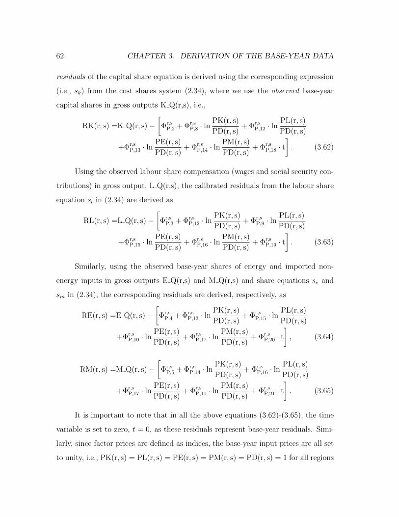
62 CHAPTER 3. DERIVATION OF THE BASE-YEAR DATA
residuals of the capital share equation is derived using the corresponding expression
(i.e., sk) from the cost shares system (2.34), where we use the observed base-year
capital shares in gross outputs K Q(r,s), i.e.,
RK(r, s) =K Q(r, s)−[Φr,s
P,2 + Φr,sP,8 · ln
PK(r, s)
PD(r, s)+ Φr,s
P,12 · lnPL(r, s)
PD(r, s)
+Φr,sP,13 · ln
PE(r, s)
PD(r, s)+ Φr,s
P,14 · lnPM(r, s)
PD(r, s)+ Φr,s
P,18 · t]. (3.62)
Using the observed labour share compensation (wages and social security con-
tributions) in gross output, L Q(r,s), the calibrated residuals from the labour share
equation sl in (2.34) are derived as
RL(r, s) =L Q(r, s)−[Φr,s
P,3 + Φr,sP,12 · ln
PK(r, s)
PD(r, s)+ Φr,s
P,9 · lnPL(r, s)
PD(r, s)
+Φr,sP,15 · ln
PE(r, s)
PD(r, s)+ Φr,s
P,16 · lnPM(r, s)
PD(r, s)+ Φr,s
P,19 · t]. (3.63)
Similarly, using the observed base-year shares of energy and imported non-
energy inputs in gross outputs E Q(r,s) and M Q(r,s) and share equations se and
sm in (2.34), the corresponding residuals are derived, respectively, as
RE(r, s) =E Q(r, s)−[Φr,s
P,4 + Φr,sP,13 · ln
PK(r, s)
PD(r, s)+ Φr,s
P,15 · lnPL(r, s)
PD(r, s)
+Φr,sP,10 · ln
PE(r, s)
PD(r, s)+ Φr,s
P,17 · lnPM(r, s)
PD(r, s)+ Φr,s
P,20 · t], (3.64)
RM(r, s) =M Q(r, s)−[Φr,s
P,5 + Φr,sP,14 · ln
PK(r, s)
PD(r, s)+ Φr,s
P,16 · lnPL(r, s)
PD(r, s)
+Φr,sP,17 · ln
PE(r, s)
PD(r, s)+ Φr,s
P,11 · lnPM(r, s)
PD(r, s)+ Φr,s
P,21 · t]. (3.65)
It is important to note that in all the above equations (3.62)-(3.65), the time
variable is set to zero, t = 0, as these residuals represent base-year residuals. Simi-
larly, since factor prices are defined as indices, the base-year input prices are all set
to unity, i.e., PK(r, s) = PL(r, s) = PE(r, s) = PM(r, s) = PD(r, s) = 1 for all regions
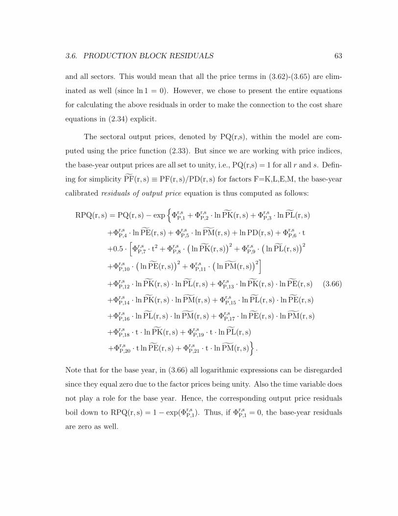
3.6. PRODUCTION BLOCK RESIDUALS 63
and all sectors. This would mean that all the price terms in (3.62)-(3.65) are elim-
inated as well (since ln 1 = 0). However, we chose to present the entire equations
for calculating the above residuals in order to make the connection to the cost share
equations in (2.34) explicit.
The sectoral output prices, denoted by PQ(r,s), within the model are com-
puted using the price function (2.33). But since we are working with price indices,
the base-year output prices are all set to unity, i.e., PQ(r,s) = 1 for all r and s. Defin-
ing for simplicity PF(r, s) ≡ PF(r, s)/PD(r, s) for factors F=K,L,E,M, the base-year
calibrated residuals of output price equation is thus computed as follows:
RPQ(r, s) = PQ(r, s)− exp
Φr,sP,1 + Φr,s
P,2 · ln PK(r, s) + Φr,sP,3 · ln PL(r, s)
+Φr,sP,4 · ln PE(r, s) + Φr,s
P,5 · ln PM(r, s) + ln PD(r, s) + Φr,sP,6 · t
+0.5 ·[Φr,s
P,7 · t2 + Φr,s
P,8 ·(
ln PK(r, s))2
+ Φr,sP,9 ·
(ln PL(r, s)
)2
+Φr,sP,10 ·
(ln PE(r, s)
)2+ Φr,s
P,11 ·(
ln PM(r, s))2]
+Φr,sP,12 · ln PK(r, s) · ln PL(r, s) + Φr,s
P,13 · ln PK(r, s) · ln PE(r, s) (3.66)
+Φr,sP,14 · ln PK(r, s) · ln PM(r, s) + Φr,s
P,15 · ln PL(r, s) · ln PE(r, s)
+Φr,sP,16 · ln PL(r, s) · ln PM(r, s) + Φr,s
P,17 · ln PE(r, s) · ln PM(r, s)
+Φr,sP,18 · t · ln PK(r, s) + Φr,s
P,19 · t · ln PL(r, s)
+Φr,sP,20 · t ln PE(r, s) + Φr,s
P,21 · t · ln PM(r, s).
Note that for the base year, in (3.66) all logarithmic expressions can be disregarded
since they equal zero due to the factor prices being unity. Also the time variable does
not play a role for the base year. Hence, the corresponding output price residuals
boil down to RPQ(r, s) = 1− exp(Φr,sP,1). Thus, if Φr,s
P,1 = 0, the base-year residuals
are zero as well.

64 CHAPTER 3. DERIVATION OF THE BASE-YEAR DATA
3.7 Labour market block residuals
We start with computing the base-year residuals from the wage curves given in
(2.40). Let RWEM(r,s,sk) be the base-year residuals of the equations of wages per
employee of skill type sk=high, medium (med), low. The wages per employee by
skill type are denoted by WEM(r,s,sk), which for the base year are obtained from the
socio-economic accounts of the WIOD database. The estimates of the parameters
of the wage curves are contained in the coefficient matrix Φr,skillW,coefficient that includes
the values of τ ’s reported in Table 2.6. Next, let Pcon(r) be the consumer price
index, which for the base year is set to unity and otherwise is endogenously derived
within the FIDELIO model. Further, let HrWktot(r) be the total hours worked by
employees of region r which for the base-year calculations also come from the socio-
economic accounts of the WIOD database. Finally denoting unemployment rates by
skill type as UNEMR(r,sk) and the regional real output by QReal(r), the residuals
of the wage curves (2.40) are obtained as
RWEM(r, s, sk)= ln WEM(r, s, sk)− Φr,skW,1 · ln
[QReal(r)/HtWktot(r)
]−Φr,sk
W,2 · Pcon(r)− Φr,skW,3 · ln UNEMR(r, sk). (3.67)
Next, the estimates of the parameters of the labour price (wage) function
(2.37) are included in the labour block coefficient matrix Φr,sL,coefficient. That is,
(Φr,sL,1,Φ
r,sL,2, . . . ,Φ
r,sL,10)′ = (β0, βl, βh, α1, α2, γll, γhh, γlh, ρtl, ρth)
′. The overall labour
hourly wage is denoted by WHRtot(r, s), and, similar to the hourly wages by skill
types WHR(r,s,sk) and wages per employee WEM(r,s,sk) is also obtained/computed
from the socio-economic accounts of the WIOD database. The base year calibrated
residuals of the labour skill type share equation are derived using (2.38), where
we use the observed high-, medium- and low-skilled labour shares denoted, respec-
tively, by LH L(r,s), LM L(r,s) and LL L(r,s). Hence, the residuals from the low-
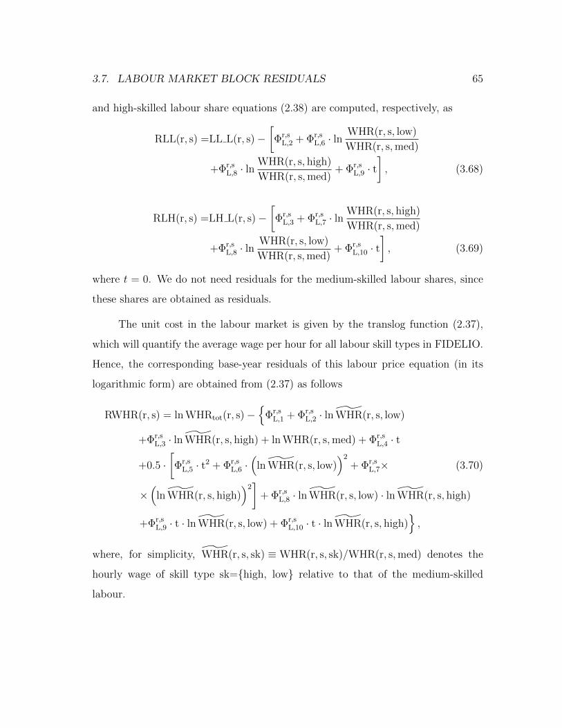
3.7. LABOUR MARKET BLOCK RESIDUALS 65
and high-skilled labour share equations (2.38) are computed, respectively, as
RLL(r, s) =LL L(r, s)−[Φr,s
L,2 + Φr,sL,6 · ln
WHR(r, s, low)
WHR(r, s,med)
+Φr,sL,8 · ln
WHR(r, s, high)
WHR(r, s,med)+ Φr,s
L,9 · t], (3.68)
RLH(r, s) =LH L(r, s)−[Φr,s
L,3 + Φr,sL,7 · ln
WHR(r, s, high)
WHR(r, s,med)
+Φr,sL,8 · ln
WHR(r, s, low)
WHR(r, s,med)+ Φr,s
L,10 · t], (3.69)
where t = 0. We do not need residuals for the medium-skilled labour shares, since
these shares are obtained as residuals.
The unit cost in the labour market is given by the translog function (2.37),
which will quantify the average wage per hour for all labour skill types in FIDELIO.
Hence, the corresponding base-year residuals of this labour price equation (in its
logarithmic form) are obtained from (2.37) as follows
RWHR(r, s) = ln WHRtot(r, s)−
Φr,sL,1 + Φr,s
L,2 · ln WHR(r, s, low)
+Φr,sL,3 · ln WHR(r, s, high) + ln WHR(r, s,med) + Φr,s
L,4 · t
+0.5 ·[Φr,s
L,5 · t2 + Φr,s
L,6 ·(
ln WHR(r, s, low))2
+ Φr,sL,7× (3.70)
×(
ln WHR(r, s, high))2]
+ Φr,sL,8 · ln WHR(r, s, low) · ln WHR(r, s, high)
+Φr,sL,9 · t · ln WHR(r, s, low) + Φr,s
L,10 · t · ln WHR(r, s, high),
where, for simplicity, WHR(r, s, sk) ≡WHR(r, s, sk)/WHR(r, s,med) denotes the
hourly wage of skill type sk=high, low relative to that of the medium-skilled
labour.
66 CHAPTER 3. DERIVATION OF THE BASE-YEAR DATA
3.8 Other relevant exogenous data
The theoretical model in the consumption block of FIDELIO is based on inter-
temporal optimization problem of households with durable and non-durable com-
modities (for details, see Luego-Prado, 2006). A very crucial feature of this model is
consideration of a collateralized constraints imposed on consumers. The last includes
a down payment requirement parameter, θ ∈ [0, 1], which represents the fraction of
durables that a household is not allowed to finance. Hence, the borrowing limit (or
maximum loan) of the individual is equal to (1− θ) fraction (share) of the stocks of
durable commodities. The mentioned constraint then implies that, at any point in
time, a household is only required to keep an accumulated durable equity equal to
θ fraction of the durables stocks. The time series of down payment requirement is
denoted by Tht(r,t) and treated as exogenous in the simulations. The corresponding
estimates are derived from (1 − θ), which is calculated as the relationship of long
term debt to the total stock of durables. Some of the base year examples used in
the model simulations are: Tht(AUT)=0.709, Tht(DNK)=0.489, Tht(DEU)=0.650,
and Tht(LVA)=0.999. In general, these parameters are close to unity, implying the
shortage of financing for purchases of durable commodities.
Interest rates (relevant) for capital costs of firms and households’ durables
purchases are considered as given in the model and are denoted by IntD(r). This
rate is taken exogenous in FIDELIO, which is basically determined by the monetary
policy. The corresponding values are mainly within the interval [0.03, 0.04] except
for a few cases, e.g., for Romania the interest rate for durable purchases is 0.07.
These data are the benchmark interest rates in the corresponding bond markets.
Efficiencies of electrical appliances, heating equipment and transport are de-
noted by CEF(r,c). For example, for the base year of 2005 these efficiencies are as-
sumed (or estimated) to be CEF(r,Electricity) = 1.1, CEF(r,Heating) = 1.05, and
3.8. OTHER RELEVANT EXOGENOUS DATA 67
CEF(r,PrivateTransport) = CEF(r,PublicTransport) = 1 for all regions r. From
2009 onwards it is assumed that all these efficiencies increase by the same rate as
between 2007 and 2008.
Depreciation rates of stocks of durable commodities are denoted as DPR(r,cd).
Since the category ‘Other Durables’ has been treated as exogenous and equal to its
base-year level, depreciation rates are defined for the other four durable commodities
Housing, Appliances, Vehicles, Video and Audio and for their aggregate ‘Total
Durables’ (for simplicity, denoted by TotD). It has been assumed that for all r and
t, the depreciation rates are equal to 0.083, 0.2, 0.015 and 0.05, respectively, for
durables Vehicle, VideoAudio, Housing and Appliances. However, the depreciation
rate of total stocks of durables TotD is endogenous because it is the weighted average
of the four exogenous depreciation rates with weights equal to the shares of the
corresponding endogenous stocks of durables in the total of the four durable stocks.
It ranges, in general, within the interval [0.02, 0.03].
Aggregate depreciation rates by sector are denoted by DPRS(r,s,t). These rates
are based on the capital input data from the EUKLEMS database, which include
information on the depreciation rates by asset and the capital stock for each asset
by industry. The asset structure of the capital stock by industry has been used for
weighting together the depreciation rates by asset in each sector.
In order to obtain the consumption demands for housing additionally the fol-
lowing data is required:
Pop(r) = Population size of region r,
Rent Pop(r) = Ratio of rented houses stocks in real terms per person in region r,
Phouse(r) = House price in region r,
SprHouse(r) = Spread of housing interest rates from those of consumer durables,
SprAsset(r) = Spread of interest rates on assets from those of consumer durables.
68 CHAPTER 3. DERIVATION OF THE BASE-YEAR DATA
For derivation of aggregate indicators of households’ financial status the fol-
lowing data is needed:
PenH(r) = pension funds of households,
CapTranH(r) = capital transfers,
DLiabH(r) = change in other liabilities except debt from year t− 1 to t,
TransfH(r) = governmental transfers,
DeprH(r) = depreciation accruing to households (for self-employed persons),
OthIncH(r) = other income of households.
For the labour market analyses, an important exogenous policy variable is
working time per employee, which is denoted by WKTM(r, s) for each region r and
sector s. In the base year they are derived by dividing the total hours worked in
each sector by the number of employees in that sector. Another exogenous variable
is labour supply rate by skill types LSR(r, sk), which is the proportion of labour
supply (labour force) in total population.

Chapter 4
FIDELIO equations
In this chapter we present all the details of FIDELIO’s equations. For simplicity of
exposition, we will skip all the so-called “add” and “fix” terms that are present in
the actual (GAMS) code of FIDELIO equations. They, however, play crucial role
in the simulation analysis. The role of the “add” terms is simulating the effect of
exogenously adding (subtracting) some amount to (from) an endogenous variable.
For example, by setting the “add” term AX = 100 in the equation that determines
variable X, we would run a simulation of the model economy when X was 100
units higher than it would be implied by the equation for X alone. The role of the
“fix” terms is exogenizing (part of) certain endogenous variables. For example, if
we have (or activate) the “fix” variable FX(sector1) = 10, then the value of X for
sector 1 would be fixed at the level of 10, while those for all other sectors would
be determined endogenously. Although the “add” and “fixed” terms are skipped,
the symbol (*) is added to the equation number indicating that the corresponding
equation has at least one of these two terms.
Throughout this chapter we stick to the following rules. An underlined variable
indicates that the corresponding variable is exogenously given, hence its value does
69
70 CHAPTER 4. FIDELIO EQUATIONS
not change in the simulation analysis. All the variables that have been used/defined
in the previous sections are, generally, different from the the variables with the
same labels in this chapter. For example, the base-year observed make matrix is
different from MAKE in this section which is now an endogenous variable. The
base-year and simulation variables are the same only if the variable is underlined
(i.e., it is exogenous) and it has a superscript 0 indicating base year. For example,
the market share matrix MKSH defined in (3.4) is denoted as MKSH0 in the model
equations below. Any variable that is not underlined is an endogenous variable.
Coefficients estimates of various required parameters obtained from econometric
estimations are exogenous, but they are not underlined. In general for simplicity,
these are all denoted by Φregion,sector/commodityblock,coefficient . For example, Φr,s
P,5 denotes the 5-
th coefficient of the output price equation in the production block for region r and
sector s. Finally, we do not include time dimension in all the equations for simplicity
purposes; however, all the variables without time indication are assumed to be
defined for current simulation period t. Lagged variables are not underlined, though
they are all taken as given for time t’s simulation exercise. Numerical subscripts
indicate the exact lagged time of a variable.
4.1 Gross outputs
Time t Make matrix is derived using the assumption of constant market shares.
That is, using the base-year market share matrix (3.4), we first obtain
MAKE(r, g, s) = MKSH0(r, g, s) ·∑
u
GDbp(r, g, u), (4.1)
where GDbp is each user’s demand for domestically produced goods expressed in
basic prices. Hence, sectoral gross outputs in nominal terms at time t are derived
4.1. GROSS OUTPUTS 71
by summing the corresponding make matrix over its product dimension:
Q(r, s) =∑
g
MAKE(r, g, s). (4.2*)
This process of transforming users’ demands for products into sectors’ supply of
products has the following implications. First, it implies that FIDELIO is a demand-
driven model. Although supply-side shocks can be simulated as well, FIDELIO fits
better for the analysis of demand-side shocks. Second, this step of equating demand
and supply of goods makes FIDELIO different from a CGE modelling approach. In
CGE it is the changes in prices that bring about equilibrium in the markets for goods.
In FIDELIO, however, the equilibrium concept in the goods market is based on the
observed empirical regularities indicating how economies are evolving over time. It
is obvious that, in general, the base-year data, used in CGE and other modelling
frameworks, are not consistent with the concept of “economic equilibrium” in its
strict economic sense. As mentioned in Chapter 1, equilibrium in FIDELIO is given
by demand reactions at all levels of users and all types of goods or factor inputs,
and by the corresponding supply that is determined under the restrictions given at
factor markets. It is also important to note that if there is a strong evidence that
certain market shares will change in the future, these can be easily incorporated
exogenously in the model simulation exercises.
Total regional real output is obtained from
QReal(r) =∑
s
[Q(r, s)/PQ(r, s)
], (4.3)
where PQ(r, s) are output prices whose derivation is discussed in Chapter 4.8.
72 CHAPTER 4. FIDELIO EQUATIONS
4.2 Demand for intermediate and primary inputs
The intermediate and primary inputs demands at purchasers’ prices are derived
using the factor (or cost) shares equations that were obtained from the translog
cost function approach (for details, see Chapter 2.2.2). To each factor equation we
also add the corresponding base-year residuals computed in Chapter 3.6. Hence,
the factor shares of capital, labour, total energy inputs, and imported non-energy
materials are derived, respectively, from
K Q(r, s) =RK0(r, s) + Φr,sP,2 + Φr,s
P,8 · lnPK(r, s)
PD(r, s)+ Φr,s
P,12 · lnPL(r, s)
PD(r, s)
+Φr,sP,13 · ln
PE(r, s)
PD(r, s)+ Φr,s
P,14 · lnPM(r, s)
PD(r, s)+ Φr,s
P,18 · t, (4.4*)
L Q(r, s) =RL0(r, s) + Φr,sP,3 + Φr,s
P,12 · lnPK(r, s)
PD(r, s)+ Φr,s
P,9 · lnPL(r, s)
PD(r, s)
+Φr,sP,15 · ln
PE(r, s)
PD(r, s)+ Φr,s
P,16 · lnPM(r, s)
PD(r, s)+ Φr,s
P,19 · t, (4.5*)
E Q(r, s) =RE0(r, s) + Φr,sP,4 + Φr,s
P,13 · lnPK(r, s)
PD(r, s)+ Φr,s
P,15 · lnPL(r, s)
PD(r, s)
+Φr,sP,10 · ln
PE(r, s)
PD(r, s)+ Φr,s
P,17 · lnPM(r, s)
PD(r, s)+ Φr,s
P,20 · t, (4.6*)
M Q(r, s) =RM0(r, s) + Φr,sP,5 + Φr,s
P,14 · lnPK(r, s)
PD(r, s)+ Φr,s
P,16 · lnPL(r, s)
PD(r, s)
+Φr,sP,17 · ln
PE(r, s)
PD(r, s)+ Φr,s
P,11 · lnPM(r, s)
PD(r, s)+ Φr,s
P,21 · t, (4.7*)
where the base-year calibrated residuals RK0, RL0, RE0 and RM0 computed in
(3.62)-(3.65) are added to their corresponding factor shares equations. The shares
of total domestic non-energy materials in gross outputs are obtained as residuals,
i.e.,
D Q(r, s) = 1−K Q(r, s)− L Q(r, s)− E Q(r, s)−M Q(r, s). (4.8)

4.2. DEMAND FOR INTERMEDIATE AND PRIMARY INPUTS 73
Equations (4.6*)-(4.8) determine the shares of total intermediate inputs as well, i.e.,
S Q(r, s) = E Q(r, s) + M Q(r, s) + D Q(r, s). (4.9)
Multiplication of all the above cost shares with the values of gross outputs
obtained from (4.2*) gives the corresponding derived inputs demands in nominal
terms. Hence, the demands for capital, labour, energy inputs, imported non-energy
inputs, and domestic non-energy materials are determined, respectively, as
K(r, s) = K Q(r, s) ·Q(r, s), (4.10)
L(r, s) = L Q(r, s) ·Q(r, s), (4.11)
E(r, s) = E Q(r, s) ·Q(r, s), (4.12)
M(r, s) = M Q(r, s) ·Q(r, s), (4.13)
D(r, s) = D Q(r, s) ·Q(r, s). (4.14)
Using the base-year product structure matrices of energy inputs (ESTR) in
(3.25), of imported non-energy inputs (MSTR) in (3.27), of domestic non-energy
inputs (DSTR) in (3.28), and the corresponding total inputs demands from (4.12)-
(4.14), the demands for intermediate goods at purchasers’ prices of each sector are
derived as follows:
Gpp(r, g, s) =ESTR0(r, g, s) · E(r, s) + MSTR0(r, g, s) ·M(r, s)
+DSTR0(r, g, s) ·D(r, s). (4.15*)
Note that since the sum of the base-year input structure matrices over goods equals
unity, in (4.15*) we have simply allocated the aggregate intermediate energy and
non-energy inputs (4.12)-(4.14) over all intermediate products, i.e.,
∑g
Gpp(r, g, s) = E(r, s) + M(r, s) + D(r, s) = S(r, s).
74 CHAPTER 4. FIDELIO EQUATIONS
The labour demands are distinguished between different skill types, and as ex-
plained in Chapter 2.3.1 these are also derived using the translog cost approach. The
low- and high-skilled labour shares equations (2.38) with their base-year calibrated
residuals obtained from (3.68)-(3.69) are determined, respectively, as
LL L(r, s) =RLL0(r, s) + Φr,sL,2 + Φr,s
L,6 · lnWHR(r, s, low)
WHR(r, s,med)
+Φr,sL,8 · ln
WHR(r, s, high)
WHR(r, s,med)+ Φr,s
L,9 · t, (4.16)
LH L(r, s) =RLH0(r, s) + Φr,sL,3 + Φr,s
L,7 · lnWHR(r, s, high)
WHR(r, s,med)
+Φr,sL,8 · ln
WHR(r, s, low)
WHR(r, s,med)+ Φr,s
L,10 · t, (4.17)
where WHR(r, s, sk) is the wage per hour of labour skill type sk = high, medium
(med), low. The shares of the medium skilled labour demands are derived as
residuals:
LM L(r, s) = 1− LL L(r, s)− LH L(r, s). (4.18)
Multiplying the above labour skill types shares (4.16)-(4.18) by the total labour
demand (4.11) gives the derived labour demand by skill types.
Combining equations (4.2*) and (4.9) gives the total intermediate demand for
each sector at purchasers’ prices :
S(r, s) = S Q(r, s) ·Q(r, s). (4.19*)
The previous steps enable us to find total value added for each sector from
VA(r, s) = Q(r, s)− E(r, s)−M(r, s)−D(r, s). (4.20*)
Alternatively, total value added can be derived as the sum of capital and labour
demands obtained in (4.10)-(4.11), i.e., VA(r, s) = K(r, s) + L(r, s).

4.3. LABOUR MARKET EQUATIONS 75
The different components of value added are determined as follows. Wages,
social security contributions, production taxes, production subsidies, and deprecia-
tion are computed using the corresponding base-year shares given in (3.18)-(3.21),
that is,
VAC(r,wage, s) = [1− SSC L0(r, s)] · L Q(r, s) ·Q(r, s), (4.21)
VAC(r, soc.sec.cont, s) = SSC L0(r, s) · L Q(r, s) ·Q(r, s), (4.22)
VAC(r, prdn.tax, s) = TXP Q0(r, s) ·Q(r, s), (4.23)
VAC(r, prdn.sub, s) = SBP Q0(r, s) ·Q(r, s), (4.24)
VAC(r, depr, s) = DPR Q0(r, s) ·Q(r, s). (4.25)
The remaining part of the total value added then gives its last component – operating
surplus:
VAC(r,oper.surp, s) = VA(r, s)− VAC(r,wage, s)− VAC(r, soc.sec.cont, s)
−VAC(r, prdn.tax, s)− VAC(r, prdn.sub, s)− VAC(r, depr, s). (4.26)
Note that the total labour demand (4.11) can be also derived by summing wages
(2.38) and social security contributions (4.22), that is,
L(r, s) = VAC(r,wage, s) + VAC(r, soc.sec.cont, s) = L Q(r, s) ·Q(r, s).
The regional labour demand (compensation) is thus given by
LReg(r) =∑
s
[VAC(r,wage, s) + VAC(r, soc.sec.cont, s)]. (4.27*)
4.3 Labour market equations
Multiplication of total labour demand (4.11) by labour shares by skill types (4.16)-
(4.18) gives the labour demand by skill type. Dividing the last by the hourly wage by
76 CHAPTER 4. FIDELIO EQUATIONS
labour skill type (or price of labour skill type) WHR(r, s, sk) gives the total number
of hours worked by skill type sk in sector s and region r:
HRWK(r, s, sk) =[L(r, s) · SK L(r, s, sk)
]/WHR(r, s, sk). (4.28*)
where the labour skill type shares are compactly written as SK L(r, s, low) = LL L(r, s),
SK L(r, s,med) = LM L(r, s) and SK L(r, s, high) = LH L(r, s).
The total number of regional hours worked in region r is then given by
HrWktot(r) =∑
s
∑sk
HRWK(r, s, sk). (4.29)
Using hours worked by skill type (4.28*) and the exogenous variable of working
time per employee WKTM(r, s), we then derive total number of employees by skill
type in each sector and each region as follows:
EMP(r, s, sk) = HRWK(r, s, sk)/WKTM(r, s). (4.30*)
Therefore, total employment for all skill levels is
EMPtot(r, s) =∑
sk
EMP(r, s, sk). (4.31*)
Using the exogenously given labour supply rates for each skill level and popu-
lation size, labour supply by skill type is exogenously given as follows:
LSUP(r, sk) = Pop(r) · LSR(r, sk). (4.32*)
Finally, employing (4.31*) and (4.32*), unemployment rate by labour skill type
is computed as
UNEMR(r, sk) =[LSUP(r, sk)−
∑s
EMP(r, s, sk)]/LSUP(r, sk). (4.33*)
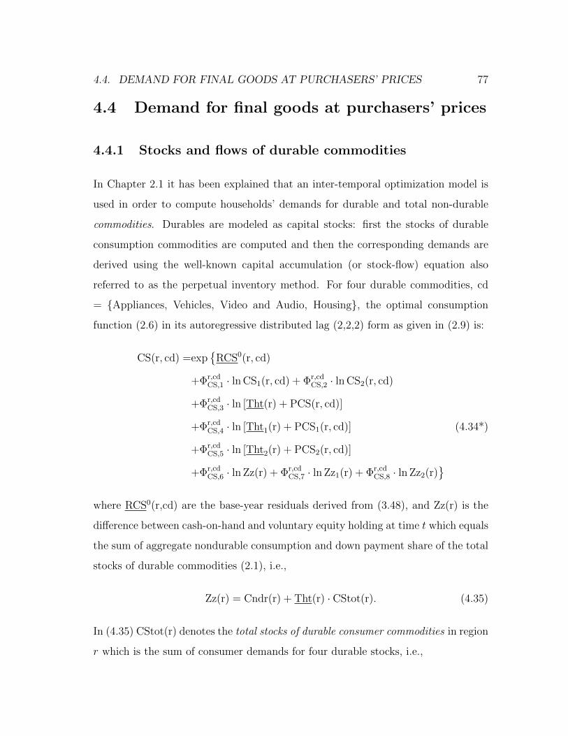
4.4. DEMAND FOR FINAL GOODS AT PURCHASERS’ PRICES 77
4.4 Demand for final goods at purchasers’ prices
4.4.1 Stocks and flows of durable commodities
In Chapter 2.1 it has been explained that an inter-temporal optimization model is
used in order to compute households’ demands for durable and total non-durable
commodities. Durables are modeled as capital stocks: first the stocks of durable
consumption commodities are computed and then the corresponding demands are
derived using the well-known capital accumulation (or stock-flow) equation also
referred to as the perpetual inventory method. For four durable commodities, cd
= Appliances, Vehicles, Video and Audio, Housing, the optimal consumption
function (2.6) in its autoregressive distributed lag (2,2,2) form as given in (2.9) is:
CS(r, cd) =exp
RCS0(r, cd)
+Φr,cdCS,1 · ln CS1(r, cd) + Φr,cd
CS,2 · ln CS2(r, cd)
+Φr,cdCS,3 · ln [Tht(r) + PCS(r, cd)]
+Φr,cdCS,4 · ln [Tht1(r) + PCS1(r, cd)] (4.34*)
+Φr,cdCS,5 · ln [Tht2(r) + PCS2(r, cd)]
+Φr,cdCS,6 · ln Zz(r) + Φr,cd
CS,7 · ln Zz1(r) + Φr,cdCS,8 · ln Zz2(r)
where RCS0(r,cd) are the base-year residuals derived from (3.48), and Zz(r) is the
difference between cash-on-hand and voluntary equity holding at time t which equals
the sum of aggregate nondurable consumption and down payment share of the total
stocks of durable commodities (2.1), i.e.,
Zz(r) = Cndr(r) + Tht(r) · CStot(r). (4.35)
In (4.35) CStot(r) denotes the total stocks of durable consumer commodities in region
r which is the sum of consumer demands for four durable stocks, i.e.,
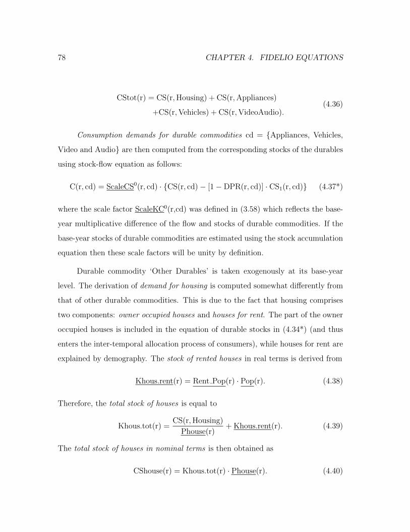
78 CHAPTER 4. FIDELIO EQUATIONS
CStot(r) = CS(r,Housing) + CS(r,Appliances)
+CS(r,Vehicles) + CS(r,VideoAudio).(4.36)
Consumption demands for durable commodities cd = Appliances, Vehicles,
Video and Audio are then computed from the corresponding stocks of the durables
using stock-flow equation as follows:
C(r, cd) = ScaleCS0(r, cd) · CS(r, cd)− [1−DPR(r, cd)] · CS1(r, cd) (4.37*)
where the scale factor ScaleKC0(r,cd) was defined in (3.58) which reflects the base-
year multiplicative difference of the flow and stocks of durable commodities. If the
base-year stocks of durable commodities are estimated using the stock accumulation
equation then these scale factors will be unity by definition.
Durable commodity ‘Other Durables’ is taken exogenously at its base-year
level. The derivation of demand for housing is computed somewhat differently from
that of other durable commodities. This is due to the fact that housing comprises
two components: owner occupied houses and houses for rent. The part of the owner
occupied houses is included in the equation of durable stocks in (4.34*) (and thus
enters the inter-temporal allocation process of consumers), while houses for rent are
explained by demography. The stock of rented houses in real terms is derived from
Khous.rent(r) = Rent Pop(r) · Pop(r). (4.38)
Therefore, the total stock of houses is equal to
Khous.tot(r) =CS(r,Housing)
Phouse(r)+ Khous.rent(r). (4.39)
The total stock of houses in nominal terms is then obtained as
CShouse(r) = Khous.tot(r) · Phouse(r). (4.40)
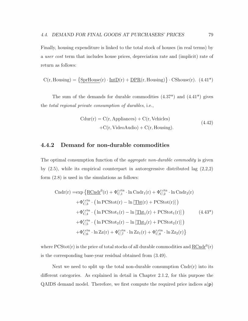
4.4. DEMAND FOR FINAL GOODS AT PURCHASERS’ PRICES 79
Finally, housing expenditure is linked to the total stock of houses (in real terms) by
a user cost term that includes house prices, depreciation rate and (implicit) rate of
return as follows:
C(r,Housing) =
SprHouse(r) · IntD(r) + DPR(r,Housing)· CShouse(r). (4.41*)
The sum of the demands for durable commodities (4.37*) and (4.41*) gives
the total regional private consumption of durables, i.e.,
Cdur(r) = C(r,Appliances) + C(r,Vehicles)
+C(r,VideoAudio) + C(r,Housing).(4.42)
4.4.2 Demand for non-durable commodities
The optimal consumption function of the aggregate non-durable commodity is given
by (2.5), while its empirical counterpart in autoregressive distributed lag (2,2,2)
form (2.8) is used in the simulations as follows:
Cndr(r) =exp
RCndr0(r) + Φr,ctnC,1 · ln Cndr1(r) + Φr,ctn
C,2 · ln Cndr2(r)
+Φr,ctnC,3 ·
(ln PCStot(r)− ln [Tht(r) + PCStot(r)]
)+Φr,ctn
C,4 ·(
ln PCStot1(r)− ln [Tht1(r) + PCStot1(r)])
(4.43*)
+Φr,ctnC,5 ·
(ln PCStot2(r)− ln [Tht2(r) + PCStot2(r)]
)+Φr,ctn
C,6 · ln Zz(r) + Φr,ctnC,7 · ln Zz1(r) + Φr,ctn
C,8 · ln Zz2(r)
where PCStot(r) is the price of total stocks of all durable commodities and RCndr0(r)
is the corresponding base-year residual obtained from (3.49).
Next we need to split up the total non-durable consumption Cndr(r) into its
different categories. As explained in detail in Chapter 2.1.2, for this purpose the
QAIDS demand model. Therefore, we first compute the required price indices a(p)
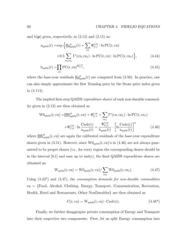
80 CHAPTER 4. FIDELIO EQUATIONS
and b(p) given, respectively, in (2.14) and (2.15) as:
aqaids(r) =exp
Ra0qaids(r) +
∑cn
Φr,cnC,1 · ln PC(r, cn)
+0.5∑
cn,cn1
Γr(cn, cn1) · ln PC(r, cn) · ln PC(r, cn1), (4.44)
bqaids(r) =∏cn
PC(r, cn)Φr,cnC,2 , (4.45)
where the base-year residuals Ra0qaids(r) are computed from (3.50). In practice, one
can also simply approximate the first Translog price by the Stone price index given
in (4.114).
The implied first-step QAIDS expenditure shares of each non-durable commod-
ity given in (2.13) are then obtained as
W0qaids(r, cn) =RW0qaids(r, cn) + Φr,cn
C,1 +∑cn1
Γr(cn, cn1) · ln PC(r, cn1)
+Φr,cnC,2 · ln
Cndr(r)
aqaids(r)+
Φr,cnC,3
bqaids(r)·[ln
Cndr(r)
aqaids(r)
]2
(4.46)
where RW0qaids(r, cn) are again the calibrated residuals of the base-year expenditure
shares given in (3.51). However, since W0qaids(r, cn)’s in (4.46) are not always guar-
anteed to be proper shares (i.e., for every region the corresponding shares should be
in the interval [0,1] and sum up to unity), the final QAIDS expenditure shares are
obtained as:
Wqaids(r, cn) = W0qaids(r, cn)/∑cn1
W0qaids(r, cn1). (4.47)
Using (4.43*) and (4.47), the consumption demands for non-durable commodities
cn = Food, Alcohol, Clothing, Energy, Transport, Communication, Recreation,
Health, Hotel and Restaurants, Other NonDurables are then obtained as
C(r, cn) = Wqaids(r, cn) · Cndr(r). (4.48*)
Finally, we further disaggregate private consumption of Energy and Transport
into their respective two components. First, let us split Energy consumption into
4.4. DEMAND FOR FINAL GOODS AT PURCHASERS’ PRICES 81
Electricity and Heating. Using the AIDS electricity share equation (2.24) and the
corresponding residuals from (3.53), we have
Welect energy(r)= RWelect0(r) + ΦrEE,1
+ΓrEE · ln
[PC(r,Elect)/CEF(r,Elect)
PC(r,Heating)/CEF(r,Heating)
](4.49)
+ΦrEE,2 · ln
[C(r,Energy)
Penergy(r)
]where the (aggregate) price of energy is the price index aenergy
aids (r) in the AIDS system
and is determined similar to (4.44), i.e.,
Penergy(r) = exp
Raenergyaids (r) + Φr
EE,1 · lnPC(r,Elect)
CEF(r,Elect)+ Φr
EE,2 · lnPC(r,Heat)
CEF(r,Heat)
+ΓrEE · ln
PC(r,Elect)
CEF(r,Elect)· ln PC(r,Heat)
CEF(r,Heat)(4.50)
+0.5 · ΓrEE ·
[(ln
PC(r,Elect)
CEF(r,Elect)
)2
+(
lnPC(r,Heat)
CEF(r,Heat)
)2],
where Raenergyaids (r) are the corresponding base-year residuals of the energy price index
equation computed in (3.52). Observe that in (4.49) and (4.50) all the prices of
energy types are adjusted for the corresponding efficiencies factors of electrical
appliances or heating equipments given in CEF matrices. In practice, one can also
simply approximate the Translog price (4.50) by the corresponding Stone price index
given in (4.116).
The consumer demands for electricity and heating are then derived, respec-
tively, as:
C(r,Elect) =Welect energy(r) · C(r,Energy), (4.51)
C(r,Heating) =C(r,Energy)− C(r,Elect). (4.52)
In this case usually an adjustment for obtaining proper shares similar to (4.47) is
not required as there are only two energy commodities, but could be done only if
the obtained share Welect energy(r) crosses [0,1] border.
82 CHAPTER 4. FIDELIO EQUATIONS
Similar to the split of Electricity from Energy commodity, we split Private
Transport from total Transport. Using the base-year residuals from the private
transport shares equation (3.56), we have
Wprivtr tran(r)= RWprivtr0(r) + ΦrTT,1
+ΓrTT · ln
[PC(r,PrivTr)/CEF(r,PrivTr)
PC(r,PubTr)/CEF(r,PubTr)
](4.53)
+ΦrTT,2 · ln
[C(r,Transport)
Ptran(r)
],
where the AIDS price index atranaids (r) defines the aggregate transport price as
Ptran(r) = exp
Ratranaids (r) + Φr
TT,1 · lnPC(r,PrivTr)
CEF(r,PrivTr)+ Φr
TT,2 · lnPC(r,PubTr)
CEF(r,PubTr)
+ΓrTT · ln
PC(r,PrivTr)
CEF(r,PrivTr)· ln PC(r,PubTr)
CEF(r,PubTr)(4.54)
+0.5 · ΓrTT ·
[(ln
PC(r,PrivTr)
CEF(r,PrivTr)
)2
+(
lnPC(r,PubTr)
CEF(r,PubTr)
)2],
with the base-year residuals Ratranaids (r) are obtained from (3.55). As with the ag-
gregate prices of all non-durables and energy, one can approximate the transport
Translog price (4.54) by the corresponding Stone price index given in (4.117).
Finally, the demands for private transport and public transport are obtained,
respectively, from
C(r,PrivTr) =Wprivtr tran(r) · C(r,Transport), (4.55)
C(r,PubTr) =C(r,Transport)− C(r,PrivTr). (4.56)
4.4.3 Sectoral demands for investments
Sectoral capital stocks, denoted by KS, are derived from the assumption that their
total user cost value is equal to the sectoral capital compensation (or cash flow),
i.e., KS(r, s) · UCKS(r, s) = K(r, s), where UCKS(r,s) is the user cost of capital by

4.4. DEMAND FOR FINAL GOODS AT PURCHASERS’ PRICES 83
sector. Since cash flow data can be negative, such sectoral base-year capital stocks
are nullified by adding the appropriate add-factors AddKS(r,s) to the obtained (neg-
ative) capital stocks. Consequently, these values are taken as given in the simulation
exercises. Hence, the equation that determines the stocks of capital by sector is
KS(r, s) = K(r, s)/UCKS(r, s) + AddKS0(r, s). (4.57*)
There are static and dynamic concepts of capital user cost, which assume that capital
market is in equilibrium in each period (for further details, see e.g., Jorgenson, 1967;
Christensen and Jorgenson, 1969). The static user cost of capital is computed from
UCKS(r, s) = PINV(r, s) ·[IntD(r) + DPRS(r, s)
], (4.58)
where IntD(r) and DPRS(r,s) are, respectively, the exogenously given interest rate
for capital costs of firms (and households’ durables purchases) and aggregate depre-
ciation rate by industry for year t, while PINV(r,s) is the price index for investments
by sector whose base-year values are all set to unity.
Alternatively, one can use the dynamic concept of capital user cost which is
based on Euler equation for capital market equilibrium and is given by
UCKS(r, s) = PINV(r, s) ·[IntD(r) + DPRS(r, s)
]−∆PINV(r, s), (4.59)
where the term ∆PINV(r, s) ≡ PINV(r, s, t)− PINV(r, s, t− 1) takes explicitly into
account changes in the investments prices from period t−1 to period t. Apparently,
it is desirable to use the dynamic version of the user cost of capital (4.59), but if
it turns out that the changes in investment prices are significantly volatile then a
switch to the static version of the user cost given in (4.58) could be more appropriate.
The investments demand by sector in purchasers’ prices is then derived using
the base-year proportion of investments in the capital stocks computed in (3.23),
i.e.,
INVpp(r, s) = I K0(r, s) ·KS(r, s). (4.60*)
84 CHAPTER 4. FIDELIO EQUATIONS
4.4.4 Demands for final products at purchasers’ prices
Region r’s private consumption demand for good g at purchasers’ prices is derived
from the corresponding COICOP commodities demands computed in Chapters 4.4.1
and 4.4.2 as follows:
Gpp(r, g, con) = AddScaleCtoP0(r, g) +
∑c BRG0(r, g, c) · C(r, c)
TotalCtoP0(r). (4.61*)
The second term on the right-hand side equation of (4.61*) is the demand for
final good g that has been adjusted using the base-year overall scale factor of
commodities-to-products transformation TotalCtoP0(r) given in (3.59). This step
of the adjustment ensures that the overall discrepancy between economy-wide total
private consumption in CPA and total COICOP commodities of the base year is
taken into account in the simulation exercises as well. Then, to this term we add
the product-specific gaps of COICOP-to-CPA consumption transformation of the
base year AddScaleCtoP0(r) from (3.60) which completes the proper transformation
process.
The investment demands for products at purchasers’ prices are obtained as
follows
Gpp(r, g, inv) =∑
s
INVpp(r, s) · ISTR0(r, g, s), (4.62*)
where INVpp(r, s) is investment demand given in (4.60*) and ISTR0(r, g, s) is the
base-year product structure of investments (3.29).
Regional public consumption and regional NPISH consumption are given ex-
ogenously as Cpubpp
(r) and Cnpishpp
(r), respectively. This allows for the possibility
of construction of a baseline scenario where these final demand components are ex-
trapolated according the regional targets for public net lending. Using these regional
totals and the corresponding product use structure of the base year, the public con-
sumption and NPISH consumption demands for products at purchasers’ prices are
4.5. DEMANDS FOR GOODS AT BASIC PRICES 85
obtained, respectively, as
Gpp(r, g, gov) = USTR0pp(r, g, gov) · Cpub
pp(r), (4.63)
Gpp(r, g, npish) = USTR0pp(r, g, npish) · Cnpish
pp(r). (4.64)
Demands for inventory are assumed to be fixed at their base-year use levels
for all products, i.e., Gpp(r, g, invent) = USEpp(r, g, invent).
And finally, demands for exports in purchasers’ prices are obtained from the
endogenous trade flows with other model regions plus the (exogenous) exports to
the rest of the world, i.e.,
Gpp(r, g, exp) = Xrate(r) ·∑r1,utr
TRDM(r1, r, g, utr)
TNCS(r1, r, g) · TRF(r1, r, g)
+
EXProw(r, g) for the baseline scenario
EXProw(r, g) ·[
PGDpp(r,g,exp)/PGrow(g)
PGD0pp(r,g,exp)/PG0
row(g)
]−TREL(r,g,exp)
otherwise(4.65*)
where TRDM(r1, r, g, utr) is the endogenous trade matrix (representing user utr’s
demands in region r1 for imports of good g produced in region r, see Chapter 4.6),
PGDpp(r, g, exp) is the FOB price of exports in the exporting region r, and PGrow(g)
is the FOB price of exports of the rest of world, and TREL’s are the trade elasticities
on the relative FOB-prices of exports. That is, the exports to the rest of the world
EXProw(r, g) computed in (3.44) are assumed to be exogenous in the base run of the
model, while in simulations these values are modified according to the relative FOB-
prices: if FOB-prices rise relative to those of the baseline scenario, then exports to
the rest of the world decreases.
4.5 Demands for goods at basic prices
To transform products demands at purchasers’ prices to demands at basic prices we
need to account for total (trade and transport) margins, and net taxes on products.

86 CHAPTER 4. FIDELIO EQUATIONS
This transformation involves three steps. First, using the base-year margin rates
paid on non-margin goods from (3.31), we determine the values of margins paid on
non-margin products as follows:
MRGpaid(r, g, u) = Gpp(r, g, u) · [1− TXSR(r, g, u)] ·MGR0paid(r, g, u), (4.66)
where the product tax net of subsidy rates are set to those of the base-year derived
in (3.30) for the baseline scenario, while could be changed for other simulation runs.
In the second step, the total margins received by margin goods are computed
using the base-year received margins shares from (3.32) as follows:
MRGrec.(r, g, u) = MGS0rec.(r, g, u) ·
∑g1
MRGpaid(r, g1, u). (4.67)
Finally, deducting the net taxes on products and paid margins (4.66) from
and adding received margins (4.67) to the demands at purchasers’ prices gives the
demands for goods at basic prices :
Gbp(r, g, u) =Gpp(r, g, u) · [1− TXSR(r, g, u)]
−MGRpaid(r, g, u) + MRGrec.(r, g, u). (4.68)
From all these steps it thus follows that margins and net taxes on products are
calculated as “mark-downs” on the demands in purchasers’ prices.
4.6 Demands for imported and domestic goods
In deriving imports demands, private consumption (CP) is treated somewhat differ-
ently than the other users. Namely, the import shares of private consumption are
obtained using the Armington approach, where these shares are a function of domes-
tic and import prices. For all other users, we use the base-year import shares matrix
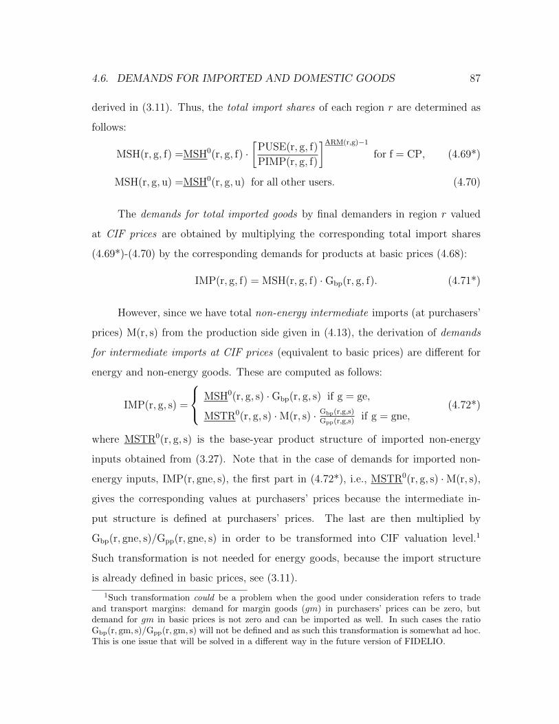
4.6. DEMANDS FOR IMPORTED AND DOMESTIC GOODS 87
derived in (3.11). Thus, the total import shares of each region r are determined as
follows:
MSH(r, g, f) =MSH0(r, g, f) ·[
PUSE(r, g, f)
PIMP(r, g, f)
]ARM(r,g)−1
for f = CP, (4.69*)
MSH(r, g, u) =MSH0(r, g, u) for all other users. (4.70)
The demands for total imported goods by final demanders in region r valued
at CIF prices are obtained by multiplying the corresponding total import shares
(4.69*)-(4.70) by the corresponding demands for products at basic prices (4.68):
IMP(r, g, f) = MSH(r, g, f) ·Gbp(r, g, f). (4.71*)
However, since we have total non-energy intermediate imports (at purchasers’
prices) M(r, s) from the production side given in (4.13), the derivation of demands
for intermediate imports at CIF prices (equivalent to basic prices) are different for
energy and non-energy goods. These are computed as follows:
IMP(r, g, s) =
MSH0(r, g, s) ·Gbp(r, g, s) if g = ge,
MSTR0(r, g, s) ·M(r, s) · Gbp(r,g,s)
Gpp(r,g,s)if g = gne,
(4.72*)
where MSTR0(r, g, s) is the base-year product structure of imported non-energy
inputs obtained from (3.27). Note that in the case of demands for imported non-
energy inputs, IMP(r, gne, s), the first part in (4.72*), i.e., MSTR0(r, g, s) ·M(r, s),
gives the corresponding values at purchasers’ prices because the intermediate in-
put structure is defined at purchasers’ prices. The last are then multiplied by
Gbp(r, gne, s)/Gpp(r, gne, s) in order to be transformed into CIF valuation level.1
Such transformation is not needed for energy goods, because the import structure
is already defined in basic prices, see (3.11).
1Such transformation could be a problem when the good under consideration refers to tradeand transport margins: demand for margin goods (gm) in purchasers’ prices can be zero, butdemand for gm in basic prices is not zero and can be imported as well. In such cases the ratioGbp(r, gm, s)/Gpp(r, gm, s) will not be defined and as such this transformation is somewhat ad hoc.This is one issue that will be solved in a different way in the future version of FIDELIO.
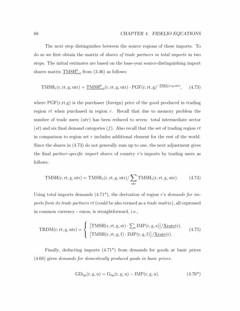
88 CHAPTER 4. FIDELIO EQUATIONS
The next step distinguishes between the source regions of these imports. To
do so we first obtain the matrix of shares of trade partners in total imports in two
steps. The initial estimates are based on the base-year source-distinguishing import
shares matrix TMSH0red from (3.46) as follows:
TMSH1(r, rt, g, utr) = TMSH0red(r, rt, g, utr) · PGF(r, rt, g)−TREL(r,g,utr), (4.73)
where PGF(r,rt,g) is the purchaser (foreign) price of the good produced in trading
region rt when purchased in region r. Recall that due to memory problem the
number of trade users (utr) has been reduced to seven: total intermediate sector
(st) and six final demand categories (f). Also recall that the set of trading region rt
in comparison to region set r includes additional element for the rest of the world.
Since the shares in (4.73) do not generally sum up to one, the next adjustment gives
the final partner-specific import shares of country r’s imports by trading users as
follows:
TMSH(r, rt, g, utr) = TMSH1(r, rt, g, utr)/∑utr
TMSH1(r, rt, g, utr). (4.74)
Using total imports demands (4.71*), the derivation of region r’s demands for im-
ports from its trade partners rt (could be also termed as a trade matrix ), all expressed
in common currency - euros, is straightforward, i.e.,
TRDM(r, rt, g, utr) =
[TMSH(r, rt, g, st) ·
∑s IMP(r, g, s)
]/Xrate(r),[
TMSH(r, rt, g, f) · IMP(r, g, f)]/Xrate(r).
(4.75)
Finally, deducting imports (4.71*) from demands for goods at basic prices
(4.68) gives demands for domestically produced goods in basic prices :
GDbp(r, g, u) = Gbp(r, g, u)− IMP(r, g, u). (4.76*)
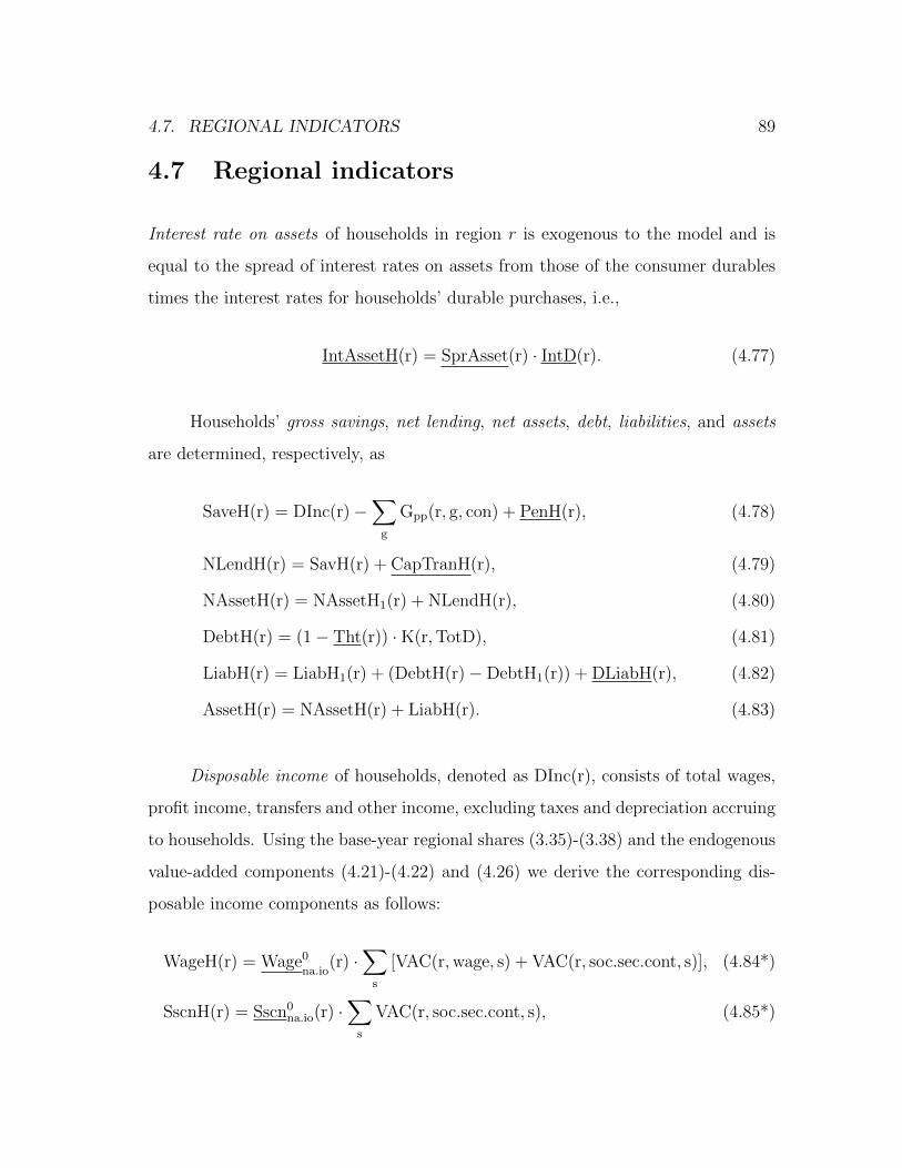
4.7. REGIONAL INDICATORS 89
4.7 Regional indicators
Interest rate on assets of households in region r is exogenous to the model and is
equal to the spread of interest rates on assets from those of the consumer durables
times the interest rates for households’ durable purchases, i.e.,
IntAssetH(r) = SprAsset(r) · IntD(r). (4.77)
Households’ gross savings, net lending, net assets, debt, liabilities, and assets
are determined, respectively, as
SaveH(r) = DInc(r)−∑
g
Gpp(r, g, con) + PenH(r), (4.78)
NLendH(r) = SavH(r) + CapTranH(r), (4.79)
NAssetH(r) = NAssetH1(r) + NLendH(r), (4.80)
DebtH(r) = (1− Tht(r)) ·K(r,TotD), (4.81)
LiabH(r) = LiabH1(r) + (DebtH(r)−DebtH1(r)) + DLiabH(r), (4.82)
AssetH(r) = NAssetH(r) + LiabH(r). (4.83)
Disposable income of households, denoted as DInc(r), consists of total wages,
profit income, transfers and other income, excluding taxes and depreciation accruing
to households. Using the base-year regional shares (3.35)-(3.38) and the endogenous
value-added components (4.21)-(4.22) and (4.26) we derive the corresponding dis-
posable income components as follows:
WageH(r) = Wage0
na.io(r) ·
∑s
[VAC(r,wage, s) + VAC(r, soc.sec.cont, s)], (4.84*)
SscnH(r) = Sscn0na.io(r) ·
∑s
VAC(r, soc.sec.cont, s), (4.85*)
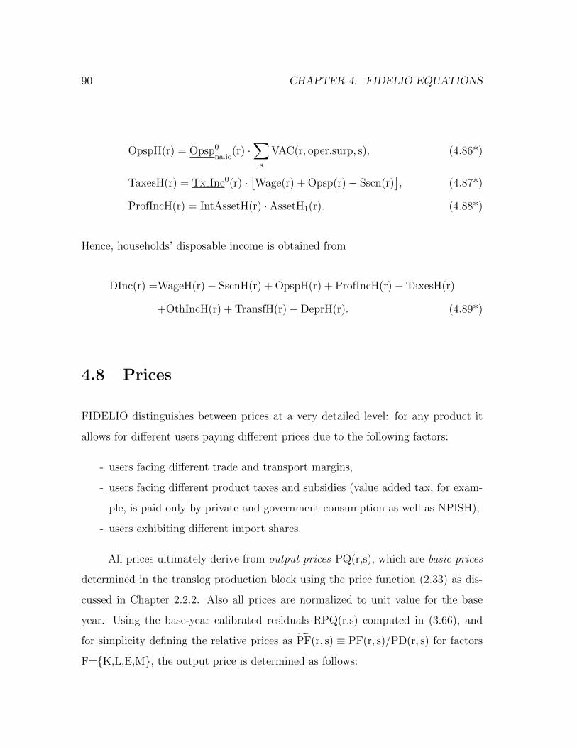
90 CHAPTER 4. FIDELIO EQUATIONS
OpspH(r) = Opsp0
na.io(r) ·
∑s
VAC(r, oper.surp, s), (4.86*)
TaxesH(r) = Tx Inc0(r) ·[Wage(r) + Opsp(r)− Sscn(r)
], (4.87*)
ProfIncH(r) = IntAssetH(r) · AssetH1(r). (4.88*)
Hence, households’ disposable income is obtained from
DInc(r) =WageH(r)− SscnH(r) + OpspH(r) + ProfIncH(r)− TaxesH(r)
+OthIncH(r) + TransfH(r)−DeprH(r). (4.89*)
4.8 Prices
FIDELIO distinguishes between prices at a very detailed level: for any product it
allows for different users paying different prices due to the following factors:
- users facing different trade and transport margins,
- users facing different product taxes and subsidies (value added tax, for exam-
ple, is paid only by private and government consumption as well as NPISH),
- users exhibiting different import shares.
All prices ultimately derive from output prices PQ(r,s), which are basic prices
determined in the translog production block using the price function (2.33) as dis-
cussed in Chapter 2.2.2. Also all prices are normalized to unit value for the base
year. Using the base-year calibrated residuals RPQ(r,s) computed in (3.66), and
for simplicity defining the relative prices as PF(r, s) ≡ PF(r, s)/PD(r, s) for factors
F=K,L,E,M, the output price is determined as follows:
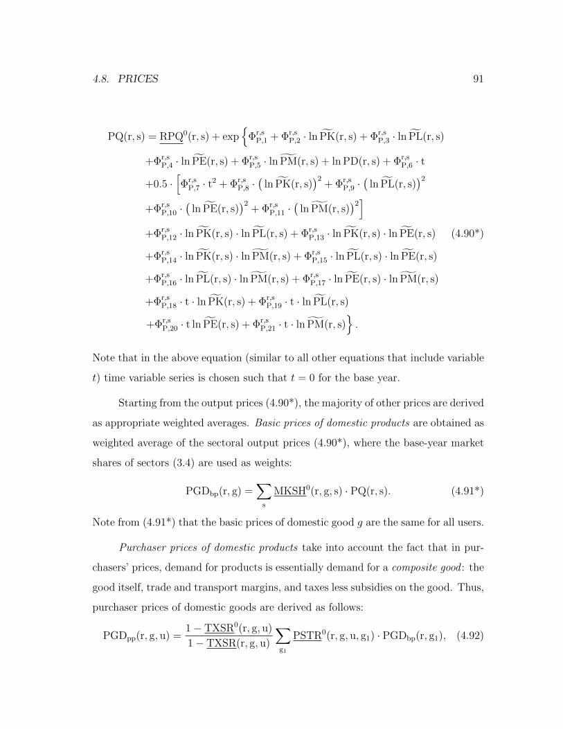
4.8. PRICES 91
PQ(r, s) = RPQ0(r, s) + exp
Φr,sP,1 + Φr,s
P,2 · ln PK(r, s) + Φr,sP,3 · ln PL(r, s)
+Φr,sP,4 · ln PE(r, s) + Φr,s
P,5 · ln PM(r, s) + ln PD(r, s) + Φr,sP,6 · t
+0.5 ·[Φr,s
P,7 · t2 + Φr,s
P,8 ·(
ln PK(r, s))2
+ Φr,sP,9 ·
(ln PL(r, s)
)2
+Φr,sP,10 ·
(ln PE(r, s)
)2+ Φr,s
P,11 ·(
ln PM(r, s))2]
+Φr,sP,12 · ln PK(r, s) · ln PL(r, s) + Φr,s
P,13 · ln PK(r, s) · ln PE(r, s) (4.90*)
+Φr,sP,14 · ln PK(r, s) · ln PM(r, s) + Φr,s
P,15 · ln PL(r, s) · ln PE(r, s)
+Φr,sP,16 · ln PL(r, s) · ln PM(r, s) + Φr,s
P,17 · ln PE(r, s) · ln PM(r, s)
+Φr,sP,18 · t · ln PK(r, s) + Φr,s
P,19 · t · ln PL(r, s)
+Φr,sP,20 · t ln PE(r, s) + Φr,s
P,21 · t · ln PM(r, s).
Note that in the above equation (similar to all other equations that include variable
t) time variable series is chosen such that t = 0 for the base year.
Starting from the output prices (4.90*), the majority of other prices are derived
as appropriate weighted averages. Basic prices of domestic products are obtained as
weighted average of the sectoral output prices (4.90*), where the base-year market
shares of sectors (3.4) are used as weights:
PGDbp(r, g) =∑
s
MKSH0(r, g, s) · PQ(r, s). (4.91*)
Note from (4.91*) that the basic prices of domestic good g are the same for all users.
Purchaser prices of domestic products take into account the fact that in pur-
chasers’ prices, demand for products is essentially demand for a composite good : the
good itself, trade and transport margins, and taxes less subsidies on the good. Thus,
purchaser prices of domestic goods are derived as follows:
PGDpp(r, g, u) =1− TXSR0(r, g, u)
1− TXSR(r, g, u)
∑g1
PSTR0(r, g, u, g1) · PGDbp(r, g1), (4.92)
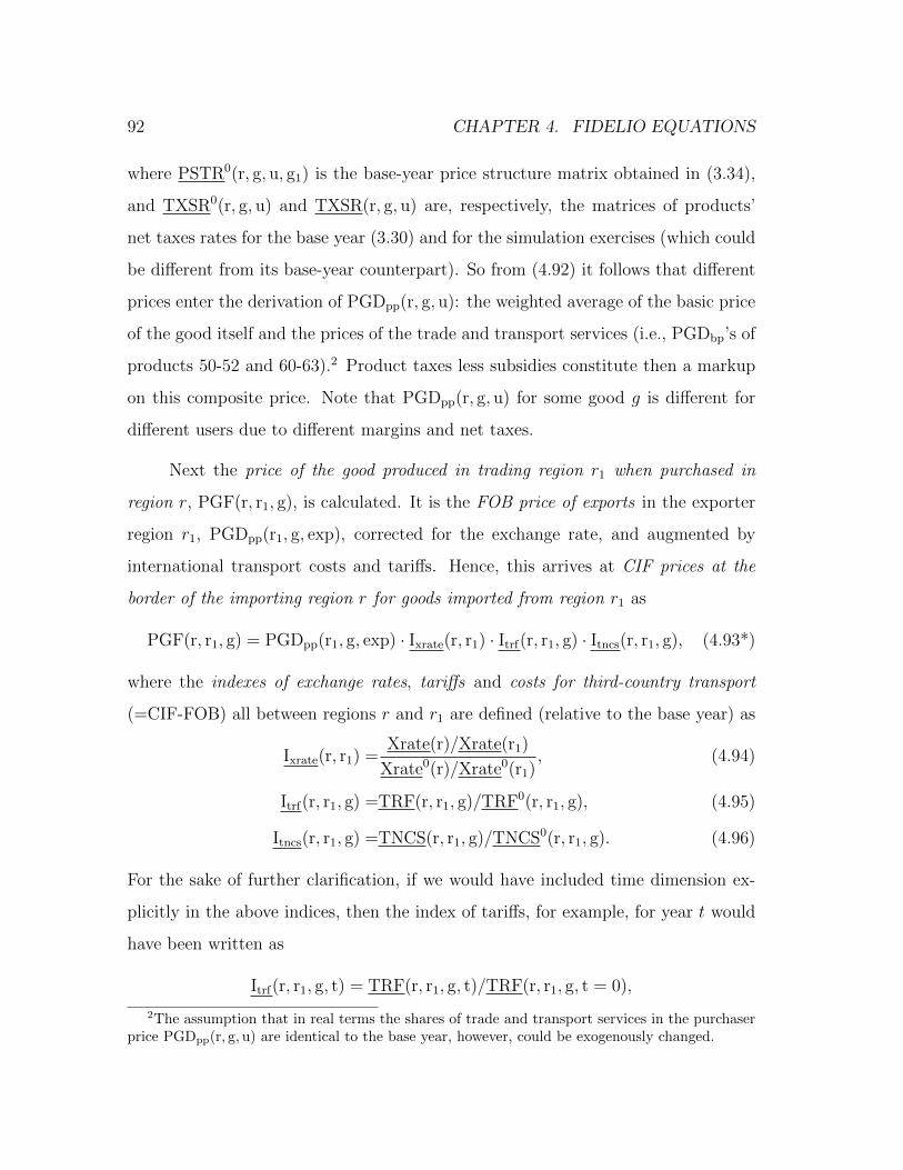
92 CHAPTER 4. FIDELIO EQUATIONS
where PSTR0(r, g, u, g1) is the base-year price structure matrix obtained in (3.34),
and TXSR0(r, g, u) and TXSR(r, g, u) are, respectively, the matrices of products’
net taxes rates for the base year (3.30) and for the simulation exercises (which could
be different from its base-year counterpart). So from (4.92) it follows that different
prices enter the derivation of PGDpp(r, g, u): the weighted average of the basic price
of the good itself and the prices of the trade and transport services (i.e., PGDbp’s of
products 50-52 and 60-63).2 Product taxes less subsidies constitute then a markup
on this composite price. Note that PGDpp(r, g, u) for some good g is different for
different users due to different margins and net taxes.
Next the price of the good produced in trading region r1 when purchased in
region r, PGF(r, r1, g), is calculated. It is the FOB price of exports in the exporter
region r1, PGDpp(r1, g, exp), corrected for the exchange rate, and augmented by
international transport costs and tariffs. Hence, this arrives at CIF prices at the
border of the importing region r for goods imported from region r1 as
PGF(r, r1, g) = PGDpp(r1, g, exp) · Ixrate(r, r1) · Itrf(r, r1, g) · Itncs(r, r1, g), (4.93*)
where the indexes of exchange rates, tariffs and costs for third-country transport
(=CIF-FOB) all between regions r and r1 are defined (relative to the base year) as
Ixrate(r, r1) =Xrate(r)/Xrate(r1)
Xrate0(r)/Xrate0(r1), (4.94)
Itrf(r, r1, g) =TRF(r, r1, g)/TRF0(r, r1, g), (4.95)
Itncs(r, r1, g) =TNCS(r, r1, g)/TNCS0(r, r1, g). (4.96)
For the sake of further clarification, if we would have included time dimension ex-
plicitly in the above indices, then the index of tariffs, for example, for year t would
have been written as
Itrf(r, r1, g, t) = TRF(r, r1, g, t)/TRF(r, r1, g, t = 0),
2The assumption that in real terms the shares of trade and transport services in the purchaserprice PGDpp(r, g,u) are identical to the base year, however, could be exogenously changed.

4.8. PRICES 93
where t = 0 represents the base year. Therefore for the base year, the CIF prices of
imports from region r1, PGF(r, r1, g), are equal to the region FOB prices of exports
PGDpp(r1, g, exp).
The corresponding CIF prices for imports from the rest of the world are taken
exogenous to the model:
PGF(r, row, g) = PGrow(g) · Ixrate(r, row) · Itrf(r, row, g) · Itncs(r, row, g), (4.97*)
where PGrow(g) is the FOB price of exports of the RoW (i.e., prices in the RoW).
Recall that the last price PGrow(g) and the purchaser price of exports of region r,
PGDpp(r, g, exp), determined demands for region r’s exports to the rest of the world
as indicated by (4.65*).
The total import CIF price at the border of region r for good g and user utr are
computed as the weighted average of the import prices of trading partners PGF’s
from (4.93*) and (4.97*) with the shares of trading partners endogenously deter-
mined in (4.73)-(4.74) as weights, i.e.,
PIMPcif(r, g, utr) =∑
rt
TMSH(r, rt, g, utr) · PGF(r, rt, g), (4.98*)
with PIMPcif(r, g, s) = PIMPcif(r, g, st) for all sectors s. Then the total import prices
including (domestic margins and) taxes less subsidies on products are derived as
follows:
PIMP(r, g, u) = PMcif(r, g, u) · 1− TXSR0(r, g, u)
1− TXSR(r, g, u). (4.99*)
The next step computes products’ use prices for all users PUSE(r, g, u), which
are the weighted averages of the purchasers’ prices of domestic products PGDpp(r, g, u)
and import prices PIMP(r, g, u) using the import shares MSH(r, g, u) from (4.69*)-
(4.70) as weights:
PUSE(r, g, u) =MSH(r, g, u) · PIMP(r, g, u)
+[1−MSH(r, g, u)] · PGDpp(r, g, u). (4.100*)
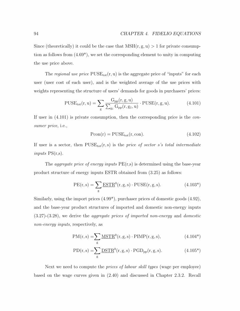
94 CHAPTER 4. FIDELIO EQUATIONS
Since (theoretically) it could be the case that MSH(r, g, u) > 1 for private consump-
tion as follows from (4.69*), we set the corresponding element to unity in computing
the use price above.
The regional use price PUSEtot(r, u) is the aggregate price of “inputs” for each
user (user cost of each user), and is the weighted average of the use prices with
weights representing the structure of users’ demands for goods in purchasers’ prices:
PUSEtot(r, u) =∑
g
Gpp(r, g, u)∑g1
Gpp(r, g1, u)· PUSE(r, g, u). (4.101)
If user in (4.101) is private consumption, then the corresponding price is the con-
sumer price, i.e.,
Pcon(r) = PUSEtot(r, con). (4.102)
If user is a sector, then PUSEtot(r, s) is the price of sector s’s total intermediate
inputs PS(r,s).
The aggregate price of energy inputs PE(r,s) is determined using the base-year
product structure of energy inputs ESTR obtained from (3.25) as follows:
PE(r, s) =∑
g
ESTR0(r, g, s) · PUSE(r, g, s). (4.103*)
Similarly, using the import prices (4.99*), purchaser prices of domestic goods (4.92),
and the base-year product structures of imported and domestic non-energy inputs
(3.27)-(3.28), we derive the aggregate prices of imported non-energy and domestic
non-energy inputs, respectively, as
PM(r, s) =∑
g
MSTR0(r, g, s) · PIMP(r, g, s), (4.104*)
PD(r, s) =∑
g
DSTR0(r, g, s) · PGDpp(r, g, s). (4.105*)
Next we need to compute the prices of labour skill types (wage per employee)
based on the wage curves given in (2.40) and discussed in Chapter 2.3.2. Recall
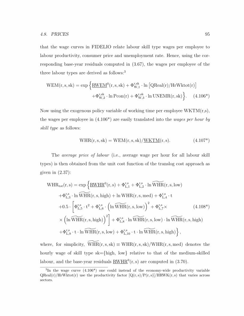
4.8. PRICES 95
that the wage curves in FIDELIO relate labour skill type wages per employee to
labour productivity, consumer price and unemployment rate. Hence, using the cor-
responding base-year residuals computed in (3.67), the wages per employee of the
three labour types are derived as follows:3
WEM(r, s, sk) = exp
RWEM0(r, s, sk) + Φr,skW,1 · ln
[QReal(r)/HrWktot(r)
]+Φr,sk
W,2 · ln Pcon(r) + Φr,skW,3 · ln UNEMR(r, sk)
. (4.106*)
Now using the exogenous policy variable of working time per employee WKTM(r,s),
the wages per employee in (4.106*) are easily translated into the wages per hour by
skill type as follows:
WHR(r, s, sk) = WEM(r, s, sk)/WKTM(r, s). (4.107*)
The average price of labour (i.e., average wage per hour for all labour skill
types) is then obtained from the unit cost function of the translog cost approach as
given in (2.37):
WHRtot(r, s) = exp
RWHR0(r, s) + Φr,sL,1 + Φr,s
L,2 · ln WHR(r, s, low)
+Φr,sL,3 · ln WHR(r, s, high) + ln WHR(r, s,med) + Φr,s
L,4 · t
+0.5 ·[Φr,s
L,5 · t2 + Φr,s
L,6 ·(
ln WHR(r, s, low))2
+ Φr,sL,7× (4.108*)
×(
ln WHR(r, s, high))2]
+ Φr,sL,8 · ln WHR(r, s, low) · ln WHR(r, s, high)
+Φr,sL,9 · t · ln WHR(r, s, low) + Φr,s
L,10 · t · ln WHR(r, s, high),
where, for simplicity, WHR(r, s, sk) ≡WHR(r, s, sk)/WHR(r, s,med) denotes the
hourly wage of skill type sk=high, low relative to that of the medium-skilled
labour, and the base-year residuals RWHR0(r, s) are computed in (3.70).
3In the wage curve (4.106*) one could instead of the economy-wide productivity variableQReal(r)/HrWktot(r) use the productivity factor [Q(r, s)/P(r, s)]/HRWK(r, s) that varies acrosssectors.
96 CHAPTER 4. FIDELIO EQUATIONS
Recall that prices are defined as indices. Thus, the average price of labour at
time t relative to that of the base year then gives the price of labour which is used
in the production block, i.e.,
PL(r, s) = WHRtot(r, s)/WHR0tot(r, s). (4.109*)
Similarly, the price of sectoral capital stock is obtained as an index of user cost of
capital – using its static concept (4.58) or the dynamic one (4.59) – as follows:
PK(r, s) = UCKS(r, s)/UCKS0(r, s). (4.110)
The prices of investments are determined from the products’ use prices for invest-
ments and the base-year product structure of investments from (3.29) as:
PINV(r, s) =∑
g
ISTR0(r, g, s) · PUSE(r, g, inv). (4.111*)
The prices of the consumption commodities (i.e., COICOP commodities) are
calculated on the base of CPA-products’ use prices for private consumption from
(4.100*) and the base-year bridge matrix:
PC(r, c) =∑
g
BRG0(r, g, c) · PUSE(r, g, con). (4.112*)
Since non-durable commodities allocation is done within the QAIDS demand
system (4.46), the aggregate price of non-durable commodities is equivalent to the
corresponding price index, i.e.,
PCndr(r) = aqaids(r) (4.113)
where aqaids(r) is computed in (4.44).4
4It is often the case that in practice instead of the correct Translog price (4.44), its approximateStone price index – a weighted sum of the relevant prices – is used. In such a case, instead of(4.113) the price of aggregate non-durable becomes
PCndr(r) =∑cn
C(r, cn)
Cndr(r)PC(r, cn), (4.114)
which is also used for aqaids(r) in the entire QAIDS system.
4.8. PRICES 97
Using (4.112*), consumption of durables (4.37*) and (4.41*), and total durable
consumption (4.42), the aggregate price of all durables is obtained from
PCdur(r) =∑cd
C(r, cd)
Cdur(r)· PC(r, cd). (4.115*)
Given that energy and transport have been allocated into their corresponding
components using the AIDS models in (4.49) and (4.53), respectively, the aggregate
prices of energy and transport are defined within these models as well. These are
already given, respectively, in (4.50) and (4.54).5
The price of all commodities from the QAIDS block is computed as
PCtot(r) =Cndr(r, c)
Ctot(r)· PCndr(r) +
Cdur(r, c)
Ctot(r)· PCdur(r), (4.118*)
where Ctot(r) = Cndr(r) + Cdur(r).
The prices of stocks of durable commodities are obtained using the user cost
concept similar to that for sectoral capital stocks as given in (4.58), i.e.,
PCS(r, cd) = PC(r, cd) · [IntD(r) + DPR(r, cd)] , (4.119)
where DPR(r, cd) are the exogenously given depreciation rates for durable commodi-
ties. Using (4.119) and the demands for stocks of durables from (4.34*) and (4.36),
the price of total stock of all durable commodities is derived as
PCStot(r) =∑cd
CS(r, cd)
CStot(r)· PCS(r, cd). (4.120)
5Similar to the aggregate price on non-durables (see fn. 4 above), here one can also use thecorresponding Stone price indices. Thus, instead of (4.50) and (4.54), the prices of energy andtransport can be also derived, respectively, from
Penergy(r)=∑
c∈Elect,Heating
C(r, c)
C(r,Energy)· PC(r, c)
CEF(r, c), (4.116)
Ptran(r)=∑
c∈PrivTr,PubTr
C(r, c)
C(r,Transport)· PC(r, c)
CEF(r, c). (4.117)
98 CHAPTER 4. FIDELIO EQUATIONS
Finally, the average depreciation rate of the stocks of all durable commodi-
ties is obtained using the exogenous depreciation rates of durable stocks and the
endogenous demands for the stocks of durables as follows:
DPRtot(r) =∑cd
CS(r, cd)
CStot(r)·DPR(r, cd). (4.121)
Chapter 5
Data sources
One of the primary data source of FIDELIO is the so-called TIMESUT database.
This database contains the TIME Series of Supply and Use Tables of each of the
EU member states for the period 1995-2007 in NACE Rev1.1/CPA 2002 (59 indus-
tries/59 commodities, for the detailed breakdown, see Tables B.1 and B.2 in the
Appendix). In this dataset for each year the following tables are available: Supply
Tables at basic prices with transformation into purchaser’s prices, Use Tables at
purchasers’ prices, Use Tables at basic prices, Trade and Transport Margin Tables
and Taxes less Subsidies Tables.1
The entire TIMESUT database is, however, not publicly available as far as
it has been compiled under an Administrative Arrangement between Eurostat and
European Commission’s Joint Research Centre with confidential information pro-
vided by many member states. Part of this information (at least, 2000-2007 annual
Supply Tables at basic prices with transformation into purchasers’ prices and Use
Tables at purchasers’ prices, and five-year Input-Output Tables differentiating be-
1Financial Intermediation Services Indirectly Measured (FISIM) were originally recorded as anextra industry in the Use tables up to 2004 for many countries. In TIMESUT, FISIM has beenredistributed among industries to harmonize with the 2005-onwards FISIM treatment approach.
99
100 CHAPTER 5. DATA SOURCES
tween domestic and imported uses) submitted by member states in order to fulfill
the ESA95 Transmission Programme (EC, 1996; EC, 2007) are available at Euro-
stat website.2 However, note that these available tables contain blank confidential
cells for some countries. The confidential information submitted by member states
was reviewed and adjusted for consistency. Whenever this information is missing, it
was estimated by means of the best methods considering the available information
(Rueda-Cantuche et al., 2013).
It should be noted that in FIDELIO, SUTs (and, in fact, the whole FIDELIO
model) are included in national currencies. Exchange rates also come from the
corresponding Eurostat dataset. Individual countries are coded according to their
ISO 3166-1 alpha-3 codes (ISO, 2006),3, while the aggregated “Rest of the World”
region is coded as ’ROW’. For trade matrix construction, total imports taken from
Eurostat import matrices have to be distributed accross all trading partners covered
in the model. For this purpose, the inter-regional use tables of the EU-funded
project World Input-Output Database (WIOD) have been used (Timmer, 2012).
WIOD database comprises 35 industries and 59 commodities. The product split is
made according to the TIMESUT database.4
The main data source for modeling the production block, which requires price
and share information on labour input, capital input, energy intermediate input, do-
mestic non-energy and imported non-energy intermediate inputs, was Socio-Economic
Accounts (SEA) files of the WIOD database (December 2011 release).5 In general,
the relevant full dataset has been constructed for the EU 23 (which includes all
EU 27 countries without Bulgaria, Cyprus, Estonia and Malta), covering the period
2See http://epp.eurostat.ec.europa.eu/portal/page/portal/esa95_supply_use_
input_tables/data/workbooks.3These codes can be found at http://unstats.un.org/unsd/tradekb/Knowledgebase/
Country-Code.4For further details about WIOD, see http://www.wiod.org/.5The socio-economic accounts in WIOD mainly come from the EUKLEMS project. For further
details about EUKLEMS, see http://www.euklems.net/.
101
1995 to 2009. For details, see Kratena and Wuger (2012). This dataset is available
in the industry classification of WIOD (35 industries).
The capital stock and investment by industry for the base year have been con-
structed using the appropriate data from the SEA accounts in the WIOD database.
The WIOD’s capital stock to output ratios at the 35 industry level are expanded to
the NACE Rev1.1 2-digit classification of FIDELIO and used for the derivation of
the base-year and one-lagged capital stock variable KS(r,s). Similarly, investment
by investing industry (NACE Rev1.1 2-digit) vectors for each country are obtained
(by using fixed investment/output ratios). These vectors represent one margin of
the investment matrices INVpp(r, g, s), which for each country r have the dimen-
sion of investing industry (NACE Rev1.1 2-digit) × investment commodity (CPA
2002, 2-digit). These matrices have been adjusted by a RAS procedure towards the
commodity vector of investment in SUTs.6 However, detailed investment matrix
was available only for Austria. Hence, the investment structure for Austria was
used as the starting point in the RAS procedure, which on the commodity side is
restricted by the investment vector from SUTs and on the sector side by WIOD (or
EUROSTAT) information on sectoral investments.
The price of capital is derived as an index of user costs of capital. The time
series of dynamic user costs, given in (4.59), shows a high variance in some EU
countries due to statistical outliers in the inflation rate of investment prices, PINV.
Therefore, the full estimation for the EU 23 has been carried out using the static user
cost concept, (4.58). The aggregate depreciation rate by industry for the EU 23 coun-
tries has been calculated based on the capital input files from the WIOD/EUKLEMS
database. These files contain the depreciation rate by asset and the capital stock
for each asset by industry. The asset structure of the capital stock by industry has
been used for weighting together the depreciation rates by asset in each industry.
6For details about the RAS procedure, see e.g., Temurshoev et al. (2013).

102 CHAPTER 5. DATA SOURCES
For calculating the capital stock in t and t − 1, depreciation rates for those EU 27
countries that were not available from the WIOD/EUKLEMS capital input files,
have been approximated by those from similar countries.
The price of labour input is calculated from the hours worked by industry in
the SEA files of the WIOD database and the values for labour compensation from
the same source.
The SEA accounts data for total intermediate inputs have been complemented
by physical and monetary energy data, constructed from the WIOD energy accounts
and the information in the International Energy Agency (IEA) Energy Prices and
Taxes.7 In the first step, the WIOD physical energy data by energy carrier from 1995
to 2009 have been combined with prices (per physical unit) by energy carrier from
the OECD energy prices and taxes. Price information for certain energy carriers
(district heating, biomass and fuelwood) had to be taken from other national data
sources. From that nominal expenditure for energy and an aggregate energy price
by industry can be calculated. In the second step, the energy inputs have been
subtracted from total intermediate inputs (from the SEA accounts in the WIOD
database) in order to derive total non-energy intermediate inputs. Next, the last
had to be split up into domestic and imported non-energy intermediates. This
has been done based on the International SUT from the WIOD database. The
full matrix of the International SUT can be divided into the part of the diagonal
matrices, corresponding to the domestic use matrix and the other matrices, by
column corresponding to the import use matrix. Prices for domestic and imported
have then been calculated by combining the deflator for total intermediate inputs
(from the SEA accounts in the WIOD database) with a deflation procedure for
imported intermediates, derived from the information in the WIOD database. This
procedure encompasses the following steps:
7Further details of the IEA statistics can be obtained from http://www.iea.org/stats/.
103
1. converting the gross output deflator (in national currency) from the SEA ac-
counts into national commodity deflators by using market share matrices,
2. converting the commodity deflator into a previous years prices (pyp) series,
3. converting the international SUT from US dollars into national currency and
then applying the commodity pyp of each sending country and the exchange
rate between the sending and the receiving country in order to generate inter-
national SUT at pyp from the perspective of the receiving country.
Then the import matrix from international SUT in national currency and
current prices is divided by the import matrix in pyp from step 3, which gives imports
in pyp by commodity and user for each country. The sum over all commodities gives
the import price (pyp) for each user, which is - in a final step - converted into an
import deflator. The price for domestic intermediates is then calculated as a residual
by assuming a Divisia price index for the aggregate intermediates price and using
total intermediates, imported and domestic intermediates at current prices for the
weights in the Divisia price index.
Data for COICOP consumption categories8, disposable income and financial
wealth of households are available for EU 27 from 1995 – 2010 (Eurostat) with
some minor data gaps which have been filled by interpolation techniques. Data for
the durable stock have been constructed by assuming lifetimes for the 4 durable
categories (audio/video goods, passenger cars, household appliances, and owner oc-
cupied dwellings with respective depreciation rates of 0.2, 0.083, 0.05 and 0.015) and
applying the perpetual inventory method (i.e., stock-flow equation) from a starting
value of the durable stock in 1995 on. For the estimation of this starting value other
statistical sources that contain information about physical measures of household
durables (ODYSSEE database, EUROCONSTRUCT) and information from Euro-
8COICOP stands for “Classification of Individual Consumption According to Purpose”; see theUnited Nations Statistics Division’s COICOP information at http://unstats.un.org/unsd/cr/registry/regcst.asp?Cl=5.
104 CHAPTER 5. DATA SOURCES
stat on unit prices in consumer and investment price measurement have been used.9
The obtained capital stock data are fully consistent wit the COICOP expenditure
data (in current prices), applying the depreciation rate according to the lifetimes.
Prices for aggregates of durables and non-durables have been derived by applying
the Divisia price index.
Eurostat financial and sectoral accounts are the primary source of disposable
household income and components (wages and operating surplus, government pay-
ments, property income), stock of household debt and stock of net financial assets.
Interest rate on assets is the calculated by relating property income of households
from sectoral accounts to net financial assets. Interest rate for user costs of durable
stock is the bond market rate or household credit prime rate. Borrowing limits
(1− θ) for each country are calculated as the relationship of long term debt to the
total stock of durables.
In general, the COICOP data (expenditure, prices) have been taken from
Eurostat, only the splitting up of energy into electricity and heating had to rely
on additional statistical sources. Electricity expenditure has been estimated by
combining IEA energy balance data (for the household sector) with IEA energy
prices. The category heating has been treated as the residual in the category Energy.
Starting from a bridge matrix between the classification of SUTs (CPA 2002, 2-digit)
and COICOP for Austria in purchaser prices, bridge matrices for the other countries
have been constructed by application of RAS. Energy efficiency indices for heating
and electrical appliances are taken from the ODYSSEE database, while TREMOVE
database10 was the primary source of the energy efficiency index for vehicles.
Finally, the SEA accounts of the WIOD database (release December 2011)
have been used to obtain the following labour market data set:
9Further information about the ODYSSEE and EUROCONSTRUCT databases can be found,respectively, at http://www.odyssee-indicators.org/ and http://www.euroconstruct.org/.
10For more information visit the website http://www.tremove.org/.

105
• labour compensation of employees by skill type (high, medium and low),
• hours worked of employees by skill type, and
• number of high-, medium- and low-skilled employees.
That, in turn, led to a calculation of hourly wages for the three types of skill. These
data have been complemented by unemployment rates for the same three skill types
from EUROSTAT.

106 CHAPTER 5. DATA SOURCES
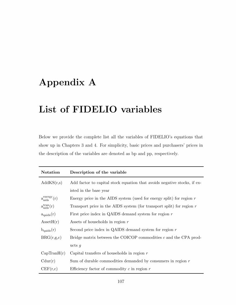
Appendix A
List of FIDELIO variables
Below we provide the complete list all the variables of FIDELIO’s equations that
show up in Chapters 3 and 4. For simplicity, basic prices and purchasers’ prices in
the description of the variables are denoted as bp and pp, respectively.
Notation Description of the variable
AddKS(r,s) Add factor to capital stock equation that avoids negative stocks, if ex-
isted in the base year
aenergyaids (r) Energy price in the AIDS system (used for energy split) for region r
atranaids (r) Transport price in the AIDS system (for transport split) for region r
aqaids(r) First price index in QAIDS demand system for region r
AssetH(r) Assets of households in region r
bqaids(r) Second price index in QAIDS demand system for region r
BRG(r,g,c) Bridge matrix between the COICOP commodities c and the CPA prod-
ucts g
CapTranH(r) Capital transfers of households in region r
Cdur(r) Sum of durable commodities demanded by consumers in region r
CEF(r,c) Efficiency factor of commodity c in region r
107

108 APPENDIX A. LIST OF FIDELIO VARIABLES
Notation Description of the variable
Cndr(r) Aggregate non-durable commodity demanded by consumers in region r
Cnpishpp(r) Regional NPISH consumption at pp
Cpubpp(r) Regional public consumption at pp
CS(r,cd) Stocks of durable consumption commodity cd demanded in region r
CShouse(r) Total stock of rented and owner occupied houses (in nominal terms)
CStot(r) Total stocks of durable consumer commodities in region r
Ctot(r) Total consumption of durable and non-durable commodities in region r
D(r,s) Total domestic non-energy inputs at pp of sector s in region r
D Q(r,s) Share of domestic non-energy inputs at pp in gross output at bp of sector
s in region r
DebtH(r) Debt of households in region r
DeprH(r) Depreciation accruing to households in region r
DInc(r) Disposable income of households in region r
DLiabH(r) Change in other households’ liabilities except debt in region r
DPR(r,cd) Depreciation rate of consumer durable cd in region r
DPR Q(r,s) Share of depreciation in gross output of sector s in region r
DPRS(r,s) Depreciation rate of capital in sector s and region r
DPRtot(r) Average depreciation rate of all consumer durables in region r
DSTR(r,g,u) Share of domestic non-energy good g in total domestic non-energy inputs
used by sector s in region r
E(r,s) Total (domestic and imported) energy inputs at pp of sector s in r
E Q(r,s) Share of total energy inputs at pp in gross output at bp of sector s in r
EMP(r,s,sk) Employment by skill type sk in sector s and region r
EMPtot(r, s) Total number of employees in sector s and region r
ESTR(r,g,s) Share of energy good g (domestic and imported) in total energy inputs
used by sector s in region r
EXProw(r, g) Exports of good g to the rest of the world (in national currency of the
exporting region)
EXProw(r, g) Region r’s exports of good g to the rest of the world
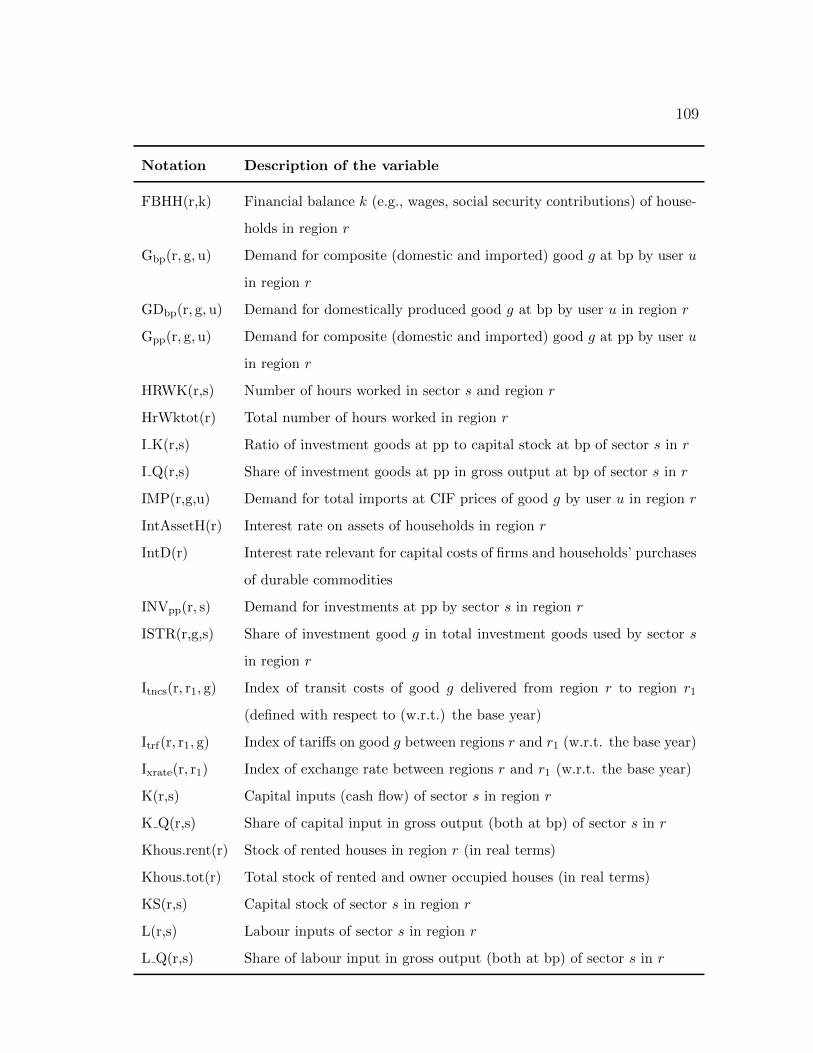
109
Notation Description of the variable
FBHH(r,k) Financial balance k (e.g., wages, social security contributions) of house-
holds in region r
Gbp(r, g,u) Demand for composite (domestic and imported) good g at bp by user u
in region r
GDbp(r, g, u) Demand for domestically produced good g at bp by user u in region r
Gpp(r, g,u) Demand for composite (domestic and imported) good g at pp by user u
in region r
HRWK(r,s) Number of hours worked in sector s and region r
HrWktot(r) Total number of hours worked in region r
I K(r,s) Ratio of investment goods at pp to capital stock at bp of sector s in r
I Q(r,s) Share of investment goods at pp in gross output at bp of sector s in r
IMP(r,g,u) Demand for total imports at CIF prices of good g by user u in region r
IntAssetH(r) Interest rate on assets of households in region r
IntD(r) Interest rate relevant for capital costs of firms and households’ purchases
of durable commodities
INVpp(r, s) Demand for investments at pp by sector s in region r
ISTR(r,g,s) Share of investment good g in total investment goods used by sector s
in region r
Itncs(r, r1, g) Index of transit costs of good g delivered from region r to region r1
(defined with respect to (w.r.t.) the base year)
Itrf(r, r1, g) Index of tariffs on good g between regions r and r1 (w.r.t. the base year)
Ixrate(r, r1) Index of exchange rate between regions r and r1 (w.r.t. the base year)
K(r,s) Capital inputs (cash flow) of sector s in region r
K Q(r,s) Share of capital input in gross output (both at bp) of sector s in r
Khous.rent(r) Stock of rented houses in region r (in real terms)
Khous.tot(r) Total stock of rented and owner occupied houses (in real terms)
KS(r,s) Capital stock of sector s in region r
L(r,s) Labour inputs of sector s in region r
L Q(r,s) Share of labour input in gross output (both at bp) of sector s in r
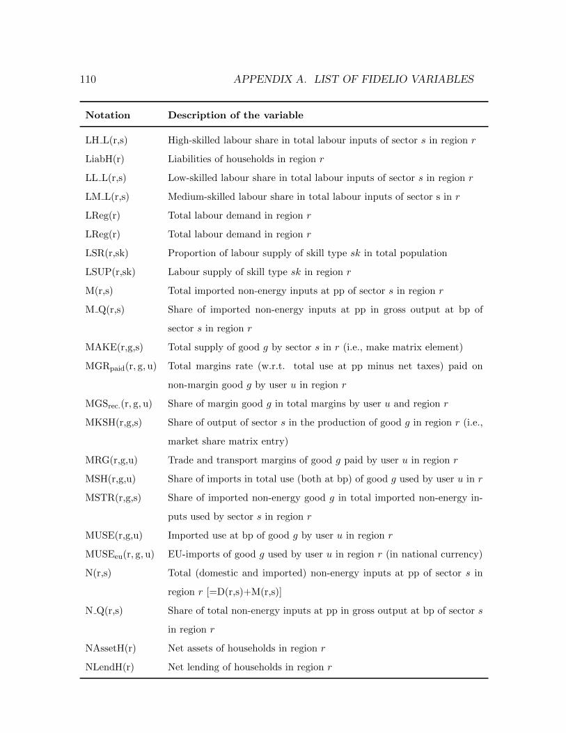
110 APPENDIX A. LIST OF FIDELIO VARIABLES
Notation Description of the variable
LH L(r,s) High-skilled labour share in total labour inputs of sector s in region r
LiabH(r) Liabilities of households in region r
LL L(r,s) Low-skilled labour share in total labour inputs of sector s in region r
LM L(r,s) Medium-skilled labour share in total labour inputs of sector s in r
LReg(r) Total labour demand in region r
LReg(r) Total labour demand in region r
LSR(r,sk) Proportion of labour supply of skill type sk in total population
LSUP(r,sk) Labour supply of skill type sk in region r
M(r,s) Total imported non-energy inputs at pp of sector s in region r
M Q(r,s) Share of imported non-energy inputs at pp in gross output at bp of
sector s in region r
MAKE(r,g,s) Total supply of good g by sector s in r (i.e., make matrix element)
MGRpaid(r, g, u) Total margins rate (w.r.t. total use at pp minus net taxes) paid on
non-margin good g by user u in region r
MGSrec.(r, g,u) Share of margin good g in total margins by user u and region r
MKSH(r,g,s) Share of output of sector s in the production of good g in region r (i.e.,
market share matrix entry)
MRG(r,g,u) Trade and transport margins of good g paid by user u in region r
MSH(r,g,u) Share of imports in total use (both at bp) of good g used by user u in r
MSTR(r,g,s) Share of imported non-energy good g in total imported non-energy in-
puts used by sector s in region r
MUSE(r,g,u) Imported use at bp of good g by user u in region r
MUSEeu(r, g,u) EU-imports of good g used by user u in region r (in national currency)
N(r,s) Total (domestic and imported) non-energy inputs at pp of sector s in
region r [=D(r,s)+M(r,s)]
N Q(r,s) Share of total non-energy inputs at pp in gross output at bp of sector s
in region r
NAssetH(r) Net assets of households in region r
NLendH(r) Net lending of households in region r

111
Notation Description of the variable
NSTR(r,g,s) Share of non-energy good g (domestic and imported) in total non-
energy inputs used by s in region r
OpspH(r) Operating surplus of households in region r
Opspna.io(r) Ratio of households’ operating surplus in national accounts to those
in input-output tables
OthIncH(r) Other income of households in region r
PC(r,c) Price of consumption commodity c in region r
PCdur(r) Aggregate price of all durable commodities in region r
PCndr(r) Aggregate price of all non-durable commodities in region r
Pcon(r) Consumer price in region r
PCS(r,cd) Price of stocks of durable commodity cd in region r
PCStot(r) Price of stock of all durable commodities in region r
PCtot(r) Aggregate price of all commodities in region r
PD(r,s) Price of domestic non-energy inputs of sector s in region r
PE(r,s) Price of energy inputs of sector s in region r
Penergy(r) Aggregate price of energy (electricity and heating) in region r
PenH(r) Pension funds of households in region r
PGDbp(r, g) Basic price of domestic good g in region r (note that this price is not
user-specific)
PGDpp(r, g, exp) FOB price of exports of good g in the exporting region r
PGDpp(r, g, u) Purchaser price of domestic good g paid by user u in region r
PGF(r, r1, g) Purchaser (foreign) price of imported good g produced in region r1
when purchased in region r; equivalently, CIF price at the border of
importing region r for good g imported from region r1
PGrow(r) FOB price of exports of the rest of the world
Phouse(r) House price in region r
PIMP(r,g,u) Total import price of good g including domestic margins and net
taxes on products
PIMPcif(r, g,utr) Total imports CIF price at the border of importing region r for good
g and user utr
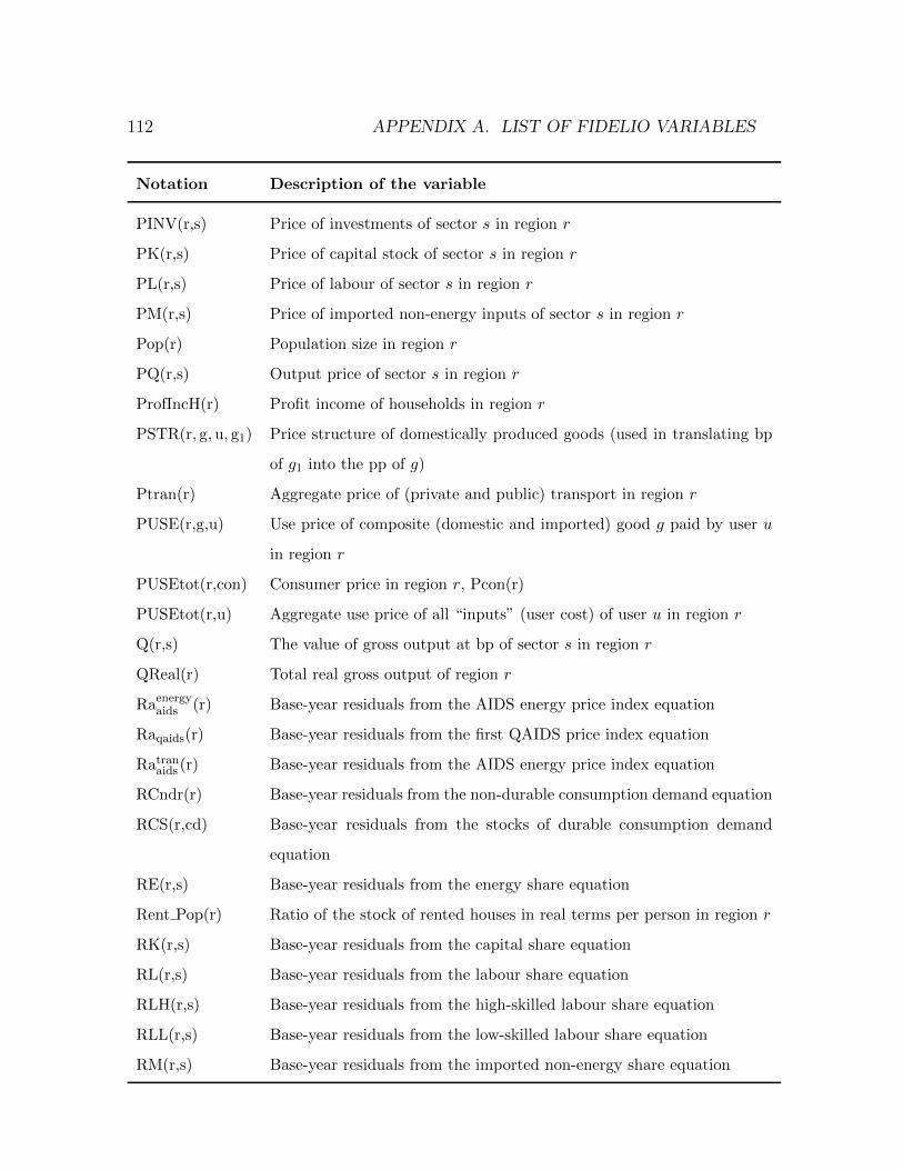
112 APPENDIX A. LIST OF FIDELIO VARIABLES
Notation Description of the variable
PINV(r,s) Price of investments of sector s in region r
PK(r,s) Price of capital stock of sector s in region r
PL(r,s) Price of labour of sector s in region r
PM(r,s) Price of imported non-energy inputs of sector s in region r
Pop(r) Population size in region r
PQ(r,s) Output price of sector s in region r
ProfIncH(r) Profit income of households in region r
PSTR(r, g,u, g1) Price structure of domestically produced goods (used in translating bp
of g1 into the pp of g)
Ptran(r) Aggregate price of (private and public) transport in region r
PUSE(r,g,u) Use price of composite (domestic and imported) good g paid by user u
in region r
PUSEtot(r,con) Consumer price in region r, Pcon(r)
PUSEtot(r,u) Aggregate use price of all “inputs” (user cost) of user u in region r
Q(r,s) The value of gross output at bp of sector s in region r
QReal(r) Total real gross output of region r
Raenergyaids (r) Base-year residuals from the AIDS energy price index equation
Raqaids(r) Base-year residuals from the first QAIDS price index equation
Ratranaids (r) Base-year residuals from the AIDS energy price index equation
RCndr(r) Base-year residuals from the non-durable consumption demand equation
RCS(r,cd) Base-year residuals from the stocks of durable consumption demand
equation
RE(r,s) Base-year residuals from the energy share equation
Rent Pop(r) Ratio of the stock of rented houses in real terms per person in region r
RK(r,s) Base-year residuals from the capital share equation
RL(r,s) Base-year residuals from the labour share equation
RLH(r,s) Base-year residuals from the high-skilled labour share equation
RLL(r,s) Base-year residuals from the low-skilled labour share equation
RM(r,s) Base-year residuals from the imported non-energy share equation
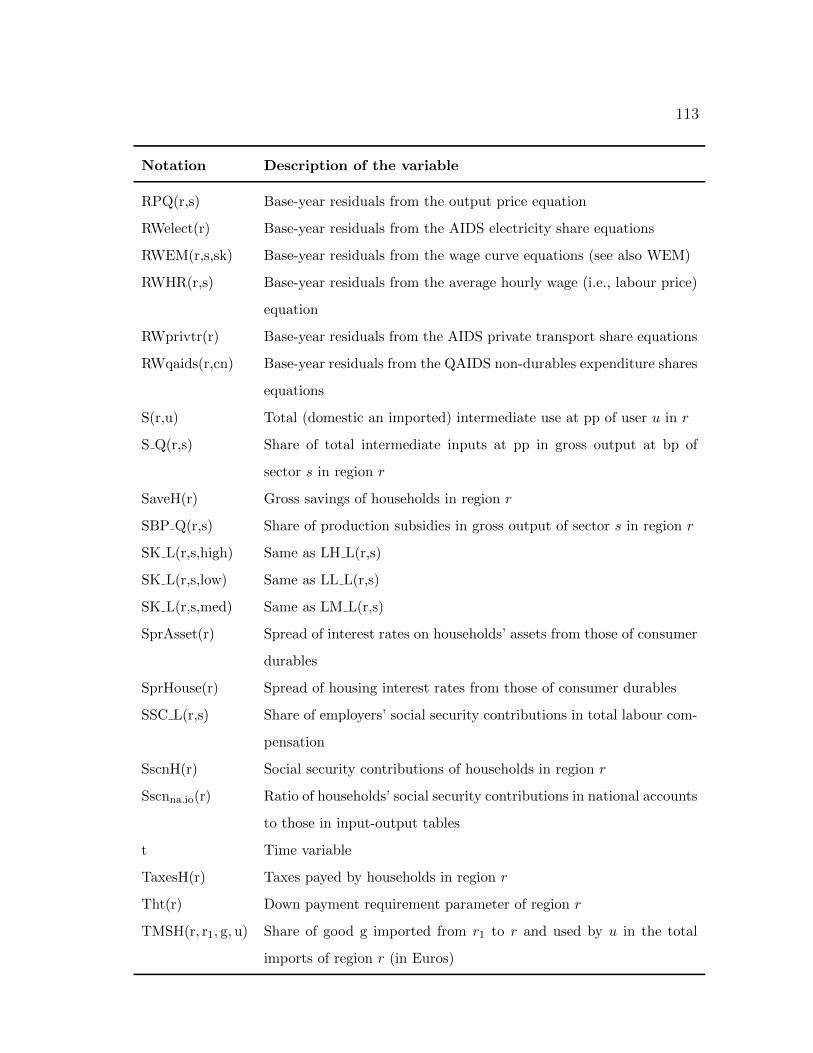
113
Notation Description of the variable
RPQ(r,s) Base-year residuals from the output price equation
RWelect(r) Base-year residuals from the AIDS electricity share equations
RWEM(r,s,sk) Base-year residuals from the wage curve equations (see also WEM)
RWHR(r,s) Base-year residuals from the average hourly wage (i.e., labour price)
equation
RWprivtr(r) Base-year residuals from the AIDS private transport share equations
RWqaids(r,cn) Base-year residuals from the QAIDS non-durables expenditure shares
equations
S(r,u) Total (domestic an imported) intermediate use at pp of user u in r
S Q(r,s) Share of total intermediate inputs at pp in gross output at bp of
sector s in region r
SaveH(r) Gross savings of households in region r
SBP Q(r,s) Share of production subsidies in gross output of sector s in region r
SK L(r,s,high) Same as LH L(r,s)
SK L(r,s,low) Same as LL L(r,s)
SK L(r,s,med) Same as LM L(r,s)
SprAsset(r) Spread of interest rates on households’ assets from those of consumer
durables
SprHouse(r) Spread of housing interest rates from those of consumer durables
SSC L(r,s) Share of employers’ social security contributions in total labour com-
pensation
SscnH(r) Social security contributions of households in region r
Sscnna.io(r) Ratio of households’ social security contributions in national accounts
to those in input-output tables
t Time variable
TaxesH(r) Taxes payed by households in region r
Tht(r) Down payment requirement parameter of region r
TMSH(r, r1, g, u) Share of good g imported from r1 to r and used by u in the total
imports of region r (in Euros)
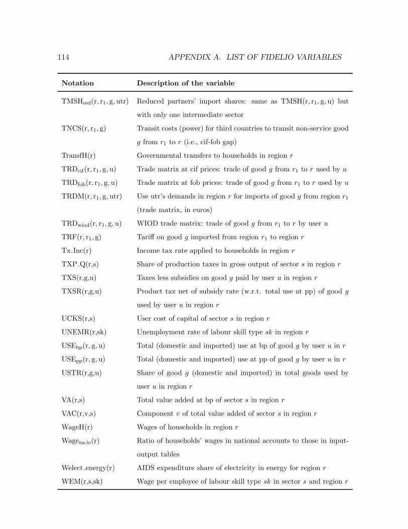
114 APPENDIX A. LIST OF FIDELIO VARIABLES
Notation Description of the variable
TMSHred(r, r1, g,utr) Reduced partners’ import shares: same as TMSH(r, r1, g,u) but
with only one intermediate sector
TNCS(r, r1, g) Transit costs (power) for third countries to transit non-service good
g from r1 to r (i.e., cif-fob gap)
TransfH(r) Governmental transfers to households in region r
TRDcif(r, r1, g,u) Trade matrix at cif prices: trade of good g from r1 to r used by u
TRDfob(r, r1, g, u) Trade matrix at fob prices: trade of good g from r1 to r used by u
TRDM(r, r1, g,utr) Use utr’s demands in region r for imports of good g from region r1
(trade matrix, in euros)
TRDwiod(r, r1, g, u) WIOD trade matrix: trade of good g from r1 to r by user u
TRF(r, r1, g) Tariff on good g imported from region r1 to region r
Tx Inc(r) Income tax rate applied to households in region r
TXP Q(r,s) Share of production taxes in gross output of sector s in region r
TXS(r,g,u) Taxes less subsidies on good g paid by user u in region r
TXSR(r,g,u) Product tax net of subsidy rate (w.r.t. total use at pp) of good g
used by user u in region r
UCKS(r,s) User cost of capital of sector s in region r
UNEMR(r,sk) Unemployment rate of labour skill type sk in region r
USEbp(r, g,u) Total (domestic and imported) use at bp of good g by user u in r
USEpp(r, g,u) Total (domestic and imported) use at pp of good g by user u in r
USTR(r,g,u) Share of good g (domestic and imported) in total goods used by
user u in region r
VA(r,s) Total value added at bp of sector s in region r
VAC(r,v,s) Component v of total value added of sector s in region r
WageH(r) Wages of households in region r
Wagena.io(r) Ratio of households’ wages in national accounts to those in input-
output tables
Welect energy(r) AIDS expenditure share of electricity in energy for region r
WEM(r,s,sk) Wage per employee of labour skill type sk in sector s and region r
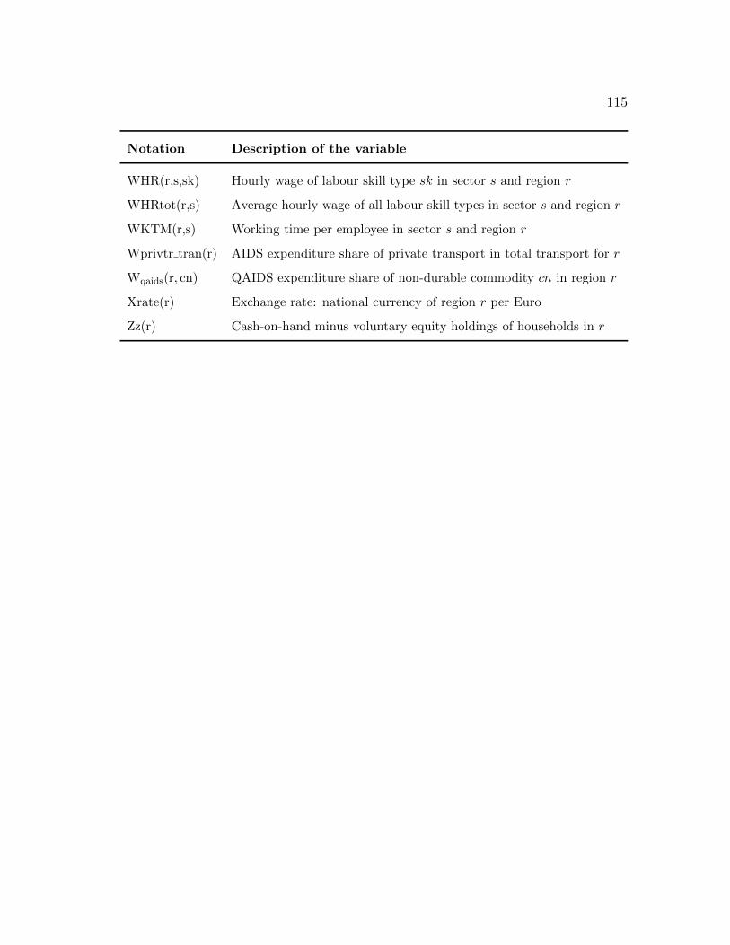
115
Notation Description of the variable
WHR(r,s,sk) Hourly wage of labour skill type sk in sector s and region r
WHRtot(r,s) Average hourly wage of all labour skill types in sector s and region r
WKTM(r,s) Working time per employee in sector s and region r
Wprivtr tran(r) AIDS expenditure share of private transport in total transport for r
Wqaids(r, cn) QAIDS expenditure share of non-durable commodity cn in region r
Xrate(r) Exchange rate: national currency of region r per Euro
Zz(r) Cash-on-hand minus voluntary equity holdings of households in r

116 APPENDIX A. LIST OF FIDELIO VARIABLES

Appendix B
Sector and product classifications
Industry classification used in FIDELIO corresponds to the statistical classification
of economic activities in the European Community, NACE Rev1.1 (EC, 2002a) and
is presented in Table B.1.1 The term NACE is derived from the French Nomenclature
statistique des activites economiques dans la Communauteuropeenne. It should be
noted that this classification is compatible with the United Nations International
Standard Industrial Classification of All Economic Activities, ISIC Rev3.1.
Products classification used in FIDELIO corresponds to the Classification of
Product by Activities, CPA (EC, 2002b) and is given in Table B.2.2 This classifica-
tion, in turn, is compatible with the United Nations Central Product Classification,
CPC Rev1.1.
1More detailed breakdown of NACE Rev1.1. can be found from http://ec.europa.eu/
eurostat/ramon/nomenclatures/index.cfm?TargetUrl=ACT_OTH_DFLT_LAYOUT&StrNom=NACE_
1_1&StrLanguageCode=EN.2Further details of CPA 2002 can be obtained from http://ec.europa.eu/eurostat/
ramon/nomenclatures/index.cfm?TargetUrl=LST_NOM_DTL&StrNom=CPA&StrLanguageCode=
EN&IntPcKey=&StrLayoutCode=HIERARCHIC.
117

118 APPENDIX B. SECTOR AND PRODUCT CLASSIFICATIONS
Table
B.1
:Statistical
classification
ofecon
omic
activities
inth
eE
urop
eanC
omm
unity,
NA
CE
Rev
1.1(E
C,
2002a)
No.
FID
EL
IOco
de
NA
CE
Rev
1.1D
escription
1sec0
1A
01A
gricultu
re,hu
ntin
gan
drela
tedserv
iceactiv
ities2
sec02
A02
Forestry,
logging
and
related
service
activ
ities3
sec05
B05
Fish
ing,
op
erating
offi
shh
atch
eriesan
dfi
shfa
rms;
service
activ
itiesin
ciden
talto
fish
ing
4sec1
0C
A10
Min
ing
of
coalan
dlig
nite;
extra
ction
of
pea
t5
sec11
CA
11E
xtra
ctionof
crud
ep
etroleu
man
dn
atu
ral
gas;
service
activ
itiesin
ciden
talto
oilan
dgas
extraction
exclu
din
gsu
rveyin
g6
sec12C
A12
Min
ing
ofu
raniu
man
dth
oriu
mores
7sec13
CB
13M
inin
gof
metal
ores8
sec14C
B14
Oth
erm
inin
gan
dqu
arry
ing
9sec15
DA
15
Man
ufa
cture
offo
od
pro
du
ctsan
db
everages
10
sec16D
A16
Man
ufa
cture
oftob
acco
pro
du
cts11
sec17D
B17
Manu
facture
oftex
tiles12
sec18D
B18
Manu
facture
ofw
earin
gap
parel;
dressin
gan
dd
yeing
of
fur
13
sec19D
C19
Tan
nin
gan
dd
ressing
of
leath
er;m
anu
factu
reof
luggage,
han
db
ags,sad
dlery,
harn
essan
dfo
otwear
14
sec20D
D20
Manu
facture
ofw
ood
an
dof
pro
du
ctsof
wood
an
dco
rk,
excep
tfu
rnitu
re;m
anu
facture
ofarticles
ofstraw
an
dp
laiting
materia
ls15
sec21
DE
21
Man
ufa
cture
ofp
ulp
,p
ap
eran
dp
ap
erp
rod
ucts
16
sec22
DE
22
Pu
blish
ing,
prin
ting
an
drep
rod
uctio
nof
record
edm
edia
17
sec23
DF
23
Man
ufa
cture
ofcok
e,refi
ned
petro
leum
pro
du
ctsan
dnu
clear
fuels
18
sec24
DG
24
Man
ufa
cture
ofch
emica
lsan
dch
emica
lp
rod
ucts
19
sec25
DH
25
Man
ufactu
reof
rub
ber
an
dp
lastic
pro
du
cts20
sec26
DI26
Man
ufactu
reof
other
non
-meta
llicm
inera
lp
rod
ucts
21
sec27
DJ27
Man
ufa
cture
ofb
asicm
etals
22
sec28
DJ28
Man
ufa
cture
offab
ricated
meta
lp
rod
ucts,
excep
tm
ach
inery
an
deq
uip
men
t23
sec29
DK
29
Man
ufa
cture
ofm
ach
inery
an
deq
uip
men
tn
.e.c.24
sec30
DL
30M
anu
facture
ofoffi
cem
ach
inery
an
dco
mpu
ters25
sec31
DL
31M
anu
facture
ofelectrica
lm
ach
inery
an
dap
para
tus
n.e.c.
26
sec32
DL
32M
anu
facture
ofrad
io,
televisio
nan
dco
mm
un
icatio
neq
uip
men
tan
dap
paratu
s27
sec33
DL
33M
anu
facture
ofm
edica
l,p
recision
an
dop
tical
instru
men
ts,w
atch
esan
dclo
cks

119
No.
FID
EL
IOco
de
NA
CE
Rev
1.1
Des
crip
tion
28se
c34
DM
34M
anu
fact
ure
ofm
oto
rve
hic
les,
trail
ers
an
dse
mi-
trail
ers
29se
c35
DM
35M
anu
fact
ure
ofoth
ertr
an
sport
equ
ipm
ent
30se
c36
DN
36M
anu
fact
ure
of
furn
itu
re;
manu
fact
uri
ng
n.e
.c.
31se
c37
DN
37R
ecycl
ing
32se
c40
E40
Ele
ctri
city
,ga
s,st
eam
an
dh
ot
wate
rsu
pp
ly33
sec4
1E
41C
olle
ctio
n,
pu
rifi
cati
on
an
ddis
trib
uti
on
of
wate
r34
sec4
5F
45C
onst
ruct
ion
35se
c50
G50
Sal
e,m
ainte
nan
cean
dre
pair
of
moto
rve
hic
les
an
dm
oto
rcycl
es;
reta
ilsa
lese
rvic
esof
au
tom
oti
vefu
el36
sec5
1G
51W
hol
esal
etr
ade
an
dco
mm
issi
on
trad
e,ex
cep
tof
moto
rveh
icle
san
dm
oto
rcycl
es37
sec5
2G
52R
etai
ltr
ade,
exce
pt
of
moto
rveh
icle
san
dm
oto
rcycl
es;
rep
air
of
per
son
al
an
dh
ou
seh
old
good
s38
sec5
5H
55H
otel
san
dre
stau
rants
39se
c60
I60
Lan
dtr
ansp
ort;
transp
ort
via
pip
elin
es40
sec6
1I6
1W
ater
tran
spor
t41
sec6
2I6
2A
irtr
ansp
ort
42se
c63
I63
Su
pp
orti
ng
and
au
xil
iary
tran
sport
act
ivit
ies;
act
ivit
ies
of
trav
elagen
cies
43se
c64
I64
Pos
tan
dte
leco
mm
un
icati
on
s44
sec6
5J65
Fin
anci
alin
term
edia
tion
,ex
cep
tin
sura
nce
an
dp
ensi
on
fun
din
g45
sec6
6J66
Insu
ran
cean
dp
ensi
on
fun
din
g,
exce
pt
com
pu
lsory
soci
al
secu
rity
46se
c67
J67
Act
ivit
ies
auxil
iary
tofi
nan
cial
inte
rmed
iati
on
47se
c70
K70
Rea
les
tate
acti
vit
ies
48se
c71
K71
Ren
tin
gof
mac
hin
ery
an
deq
uip
men
tw
ith
ou
top
erato
ran
dof
per
son
al
an
dh
ou
seh
old
good
s49
sec7
2K
72C
omp
ute
ran
dre
late
dact
ivit
ies
50se
c73
K73
Res
earc
han
ddev
elop
men
t51
sec7
4K
74O
ther
bu
sin
ess
act
ivit
ies
52se
c75
L75
Pu
bli
cad
min
istr
ati
on
an
dd
efen
ce;
com
pu
lsory
soci
al
secu
rity
53se
c80
M80
Ed
uca
tion
54se
c85
N85
Hea
lth
and
soci
al
work
55se
c90
O90
Sew
age
and
refu
sed
isp
osa
l,sa
nit
ati
on
an
dsi
mil
ar
act
ivit
ies
56se
c91
O91
Act
ivit
ies
ofm
emb
ersh
iporg
an
isati
on
n.e
.c.
57se
c92
O92
Rec
reat
ion
al,
cult
ura
lan
dsp
ort
ing
act
ivit
ies
58se
c93
O93
Oth
erse
rvic
eac
tivit
ies
59se
c95
P95
Pri
vate
hou
sehold
sw
ith
emp
loyed
per
son
s
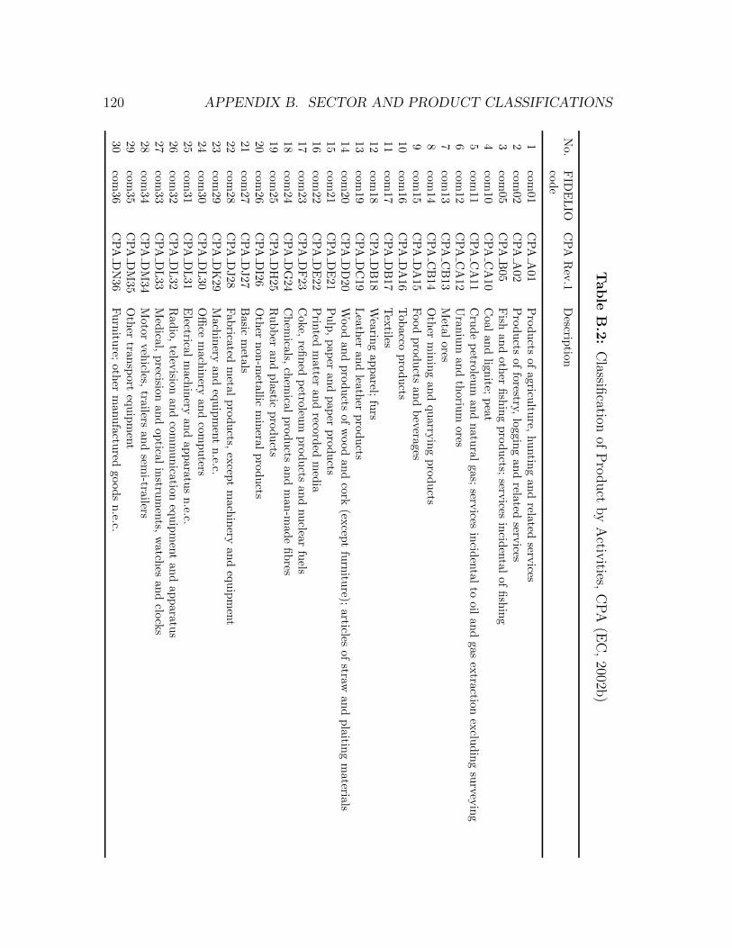
120 APPENDIX B. SECTOR AND PRODUCT CLASSIFICATIONS
Table
B.2
:C
lassification
ofP
roduct
by
Activ
ities,C
PA
(EC
,2002b
)
No.
FID
EL
IOco
de
CP
AR
ev.1
Descrip
tion
1co
m01
CP
AA
01
Pro
du
ctsof
agricultu
re,hu
ntin
gan
drela
tedserv
ices2
com02
CP
AA
02
Pro
du
ctsof
forestry,lo
ggin
gan
drela
tedserv
ices3
com05
CP
AB
05F
ishan
doth
erfi
shin
gp
rod
ucts;
services
incid
enta
lof
fish
ing
4com
10
CP
AC
A10
Coal
and
lignite;
pea
t5
com11
CP
AC
A11
Cru
de
petroleu
man
dn
atu
ral
gas;
services
incid
enta
lto
oil
and
gasex
tractionex
clud
ing
surv
eyin
g6
com12
CP
AC
A12
Ura
niu
man
dth
oriu
mores
7com
13
CP
AC
B13
Meta
lores
8com
14
CP
AC
B14
Oth
erm
inin
gan
dqu
arry
ing
pro
du
cts9
com15
CP
AD
A15
Food
pro
du
ctsan
db
everages
10com
16
CP
AD
A16
Tob
acco
pro
du
cts11
com17
CP
AD
B17
Tex
tiles12
com18
CP
AD
B18
Wearin
gap
parel;
furs
13com
19
CP
AD
C19
Leath
eran
dlea
ther
pro
du
cts14
com20
CP
AD
D20
Wood
and
pro
du
ctsof
wood
an
dco
rk(ex
cept
furn
iture);
articles
ofstraw
and
plaitin
gm
aterials15
com21
CP
AD
E21
Pu
lp,
pap
eran
dp
ap
erp
rod
ucts
16com
22
CP
AD
E22
Prin
tedm
atteran
dreco
rded
med
ia17
com23
CP
AD
F23
Coke,
refin
edp
etroleu
mp
rod
ucts
an
dnu
clear
fuels
18com
24
CP
AD
G24
Ch
emicals,
chem
ical
pro
du
ctsan
dm
an
-mad
efi
bres
19com
25
CP
AD
H25
Ru
bb
eran
dp
lastic
pro
du
cts20
com26
CP
AD
I26
Oth
ern
on-m
etallic
min
eral
pro
du
cts21
com27
CP
AD
J27
Basic
metals
22com
28
CP
AD
J28
Fab
ricatedm
etal
pro
du
cts,ex
cept
mach
inery
an
deq
uip
men
t23
com29
CP
AD
K29
Mach
inery
and
equ
ipm
ent
n.e.c.
24com
30
CP
AD
L30
Offi
cem
achin
eryan
dco
mp
uters
25com
31
CP
AD
L31
Electrical
mach
inery
and
ap
para
tus
n.e.c.
26com
32
CP
AD
L32
Rad
io,
televisio
nan
dco
mm
un
icatio
neq
uip
men
tan
dap
paratu
s27
com33
CP
AD
L33
Med
ical,p
recision
an
dop
tical
instru
men
ts,w
atch
esan
dclo
cks
28com
34
CP
AD
M34
Motor
vehicles,
trailers
an
dsem
i-trailers
29com
35
CP
AD
M35
Oth
ertran
sport
equ
ipm
ent
30com
36
CP
AD
N36
Fu
rnitu
re;oth
erm
anu
factu
redgood
sn
.e.c.
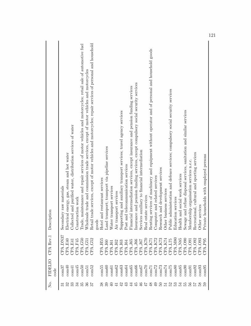
121
No.
FID
EL
IOco
de
CP
AR
ev.1
Des
crip
tion
31co
m37
CP
AD
N37
Sec
ond
ary
raw
mate
rials
32co
m40
CP
AE
40E
lect
rica
len
ergy,
gas,
stea
man
dh
ot
wate
r33
com
41C
PA
E41
Col
lect
edan
dp
uri
fied
wate
r,d
istr
ibu
tion
serv
ices
of
wate
r34
com
45C
PA
F45
Con
stru
ctio
nw
ork
35co
m50
CP
AG
50T
rad
e,m
ainte
nan
cean
dre
pair
serv
ices
of
moto
rveh
icle
san
dm
oto
rcycl
es;
reta
ilsa
leof
au
tom
oti
vefu
el36
com
51C
PA
G51
Wh
oles
ale
trad
ean
dco
mm
issi
on
trad
ese
rvic
es,
exce
pt
of
moto
rveh
icle
san
dm
oto
rcycl
es37
com
52C
PA
G52
Ret
ail
trad
ese
rvic
es,
exce
pt
of
moto
rve
hic
les
an
dm
oto
rcycl
es;
rep
air
serv
ices
of
per
son
al
an
dh
ou
seh
old
good
s38
com
55C
PA
H55
Hot
elan
dre
stau
rant
serv
ices
39co
m60
CP
AI6
0L
and
tran
sport
;tr
an
sport
via
pip
elin
ese
rvic
es40
com
61C
PA
I61
Wat
ertr
ansp
ort
serv
ices
41co
m62
CP
AI6
2A
irtr
ansp
ort
serv
ices
42co
m63
CP
AI6
3S
up
por
tin
gan
dau
xil
iary
tran
sport
serv
ices
;tr
avel
agen
cyse
rvic
es43
com
64C
PA
I64
Pos
tan
dte
leco
mm
un
icati
on
serv
ices
44co
m65
CP
AJ65
Fin
anci
alin
term
edia
tion
serv
ices
,ex
cep
tin
sura
nce
an
dp
ensi
on
fun
din
gse
rvic
es45
com
66C
PA
J66
Insu
ran
cean
dp
ensi
on
fun
din
gse
rvic
es,
exce
pt
com
pu
lsory
soci
al
secu
rity
serv
ices
46co
m67
CP
AJ67
Ser
vic
esau
xil
iary
tofi
nan
cial
inte
rmed
iati
on
47co
m70
CP
AK
70R
eal
esta
tese
rvic
es48
com
71C
PA
K71
Ren
tin
gse
rvic
esof
mach
iner
yan
deq
uip
men
tw
ith
ou
top
erato
ran
dof
per
son
al
an
dh
ou
seh
old
good
s49
com
72C
PA
K72
Com
pu
ter
and
rela
ted
serv
ices
50co
m73
CP
AK
73R
esea
rch
an
dd
evel
op
men
tse
rvic
es51
com
74C
PA
K74
Oth
erb
usi
nes
sse
rvic
es52
com
75C
PA
L75
Pu
bli
cad
min
istr
ati
on
an
dd
efen
cese
rvic
es;
com
pu
lsory
soci
al
secu
rity
serv
ices
53co
m80
CP
AM
80E
du
cati
onse
rvic
es54
com
85C
PA
N85
Hea
lth
and
soci
al
work
serv
ices
55co
m90
CP
AO
90S
ewag
ean
dre
fuse
dis
posa
lse
rvic
es,
san
itati
on
an
dsi
mil
ar
serv
ices
56co
m91
CP
AO
91M
emb
ersh
iporg
an
isati
on
serv
ices
n.e
.c.
57co
m92
CP
AO
92R
ecre
atio
nal
,cu
ltu
ral
an
dsp
ort
ing
serv
ices
58co
m93
CP
AO
93O
ther
serv
ices
59co
m95
CP
AP
95P
riva
teh
ouse
hold
sw
ith
emp
loye
dp
erso
ns

122 APPENDIX B. SECTOR AND PRODUCT CLASSIFICATIONS
Bibliography
[1] Attanasio, O.P. and G. Weber (1995), Is consumption growth consistent wiht
intertemproal optimization? Evidence from the consumer expenditure survey,
Journal of Polictical Economy, 103, pp. 1121-1157.
[2] Banerjee, A., Galbraith, J.W. and J. Dolado (1990), Dynamic specification
and linear transformations of the autoregressive-distributed lag model, Oxford
Bulletin of Economics and Statistics, 52, pp. 95-104.
[3] Banks, J., Blundell, R. and A. Lewbel (1997), Quadratic Engel curves and
consumer demands, Review of Economics and Statistics, 79, pp. 527-539.
[4] Berndt, E.R. and L.R. Christensen (1973), The translog function and the sub-
stitution of equipment, structures, and labor in U.S. manufacturing 1929-68,
Journal of Econometrics, 1, pp. 81-114.
[5] Berndt, E.R. and D.O. Wood (1975), Technology, prices and the derived de-
mand for energy, Review of Economics and Statistics, 57, pp. 259-268.
[6] Blanchflower D.G. and A.J. Oswald (1994), The Wage Curve, Cambridge, Mas-
sachusetts and London: MIT Press.
[7] Blundell, R.W. and S.R. Bond (1998), Initial conditions and moment restric-
tions in dynamic panel data models, Journal of Econometrics, 87, pp. 115-143.
123
124 BIBLIOGRAPHY
[8] Card, D. (1995), The wage curve: a review, Journal of Economic Literature,
33, pp. 785-799.
[9] Carroll, C.D. (1997), Buffer-stock saving and the life cycle/permanent ncome
hypothesis, Quarterly Journal of Economics, 112, pp. 1-55.
[10] Chen, Q., Dietzenbacher, E., Los B. and C. Yang (2010), Partially endoge-
nized consumption: A new method to incorporate the household sector into
input-output models, Paper presented at the 18th International Input-Output
Conference, Sidney, July 2010.
[11] Christensen, L.R. and W.H. Greene (1976), Economics of scale in the U.S.
electric power generation, Journal of Political Economy,84, pp. 655-676.
[12] Christensen, L.R. and D.W. Jorgenson (1969), The measurement of U.S. real
capital input, 1929-1967, Review of Income and Wealth, 15, pp. 293-320.
[13] Christensen, L.R., Jorgenson, D.W. and L.J. Lau (1973), Transcendental loga-
rithmic production frontiers, Review of Economics and Statistics, 55, pp. 28-45.
[14] Christensen, L.R., Jorgenson, D.W. and L.J. Lau (1975), Transcendental loga-
rithmic utility functions, American Economic Review, 65, pp. 367-383.
[15] Deaton, A. and J. Muellbauer (1980), An almost ideal demand system, Amer-
ican Economic Review, 70, pp. 312-326.
[16] Du Caju, P., Katay, G., Lamo, A., Nicolitsas, D. and S. Poelhekke (2010), Inter-
industry wage differentials in EU countries: What do cross-country time varying
data add to the picture?, Journal of the European Economic Association, 8, pp.
478 - 486.
[17] EC (1996), Council Regulation (EC) No 2223/96 of 25 June 1996 on the Euro-
pean system of national and regional accounts in the Community.

BIBLIOGRAPHY 125
[18] EC (2002a), Commission Regulation (EC) No 29/2002 of 19 December 2001
amending Council Regulation (EEC) No 3037/90 on the statistical classification
of economic activities in the European Community.
[19] EC (2002b), Commission Regulation No 204/2002 of 19 December 2001 amend-
ing Council Regulation (EEC) No 3696/93 on the statistical classification of
products by activity (CPA) in the European Economic Community.
[20] EC (2007), Regulation (EC) No 1392/2007 of the European Parliament and
of the Council of 13 November 2007 amending Council Regulation (EC) No
2223/96 with respect to the transmission of national accounts data.
[21] Folmer, K. (2009), Why do macro wage elasticities diverge? CBP Discussion
Paper No. 122.
[22] Goettle, R.J., Ho, M.S., Jorgenson, D.W., Slesnick, D.T. and P.J. Wilcoxen
(2007), IGEM, an inter-temporal general equilibrium model of the U.S. econ-
omy with emphasis on growth, energy and the environment, Prepared for the
U.S. Environmental Protection Agency (EPA), Office of Atmospheric Programs,
Climate Change Division, EPA Contract EP-W-05-035.
[23] Gravelle H. and R. Rees (2004), Microeconomics, 3-rd edition, London: Prentice
Hall.
[24] Greene, W.H. (2003), Econometric Analysis, 5-th edition, New Jersey: Prentice
Hall.
[25] Hall, R.E. (1978), Stochastic implications of the life cycle-permanent income
hypothesis: theory and evidence, Journal of Policitical Economy, 86, pp. 971-
987.
126 BIBLIOGRAPHY
[26] ISO (2006), International Organization for Standardization. ISO 3166-1:2006,
Codes for the representation of names of countries and their subdivisions - Part
1: Country codes.
[27] Jorgenson, D.W. (1967), The theory of investment behavior, In: Robert F.
(ed.), Determinants of Investment Behavior, MI, pp. 129-188, available at http:
//www.nber.org/chapters/c1235.
[28] Kratena, K. (2005), Prices and factor demand in an endogenized input-output
model, Economic Systems Research, 17, pp. 47-56.
[29] Kratena, K. and G. Streicher (2009), Macroeconomic input-output modelling:
structures, functional forms and closure rules, International Input-Output As-
sociation Working Paper WPIOX 09-009.
[30] Kratena, K. and M. Wuger (2010), An intertemporal optimisation model of
households in an E3-model (economy/energy/environment) framework, WIFO
Working Paper 382, WIFO, Vienna.
[31] Kratena, K. and M. Wuger (2012), Technical change and energy demand in
Europe, WIFO Working Paper 427, WIFO, Vienna.
[32] Kratena, K., Mongelli, I. and M. Wuger (2009), An econometric input-output
model for EU countries based on supply and use tables: private consumption,
International Input-Output Association Working Paper WPIOX 09-006.
[33] Lancaster, K.J. (1966), A new approach to consumer theory, Journal of Political
Economy, 74, pp. 132-157.
[34] Leontief, W.W. (1936), Quantitative input-output relations in the economic
system of the United States, Review of Economics and Statistics, 18, pp. 105-
125.
BIBLIOGRAPHY 127
[35] Leontief W.W. (1941), The Structure of American Economy, 1919-1929: An
Empirical Application of Equilibrium Analysis, Cambridge: Cambridge Univer-
sity Press.
[36] Luengo-Prado, M.J. (2006), Durables, nondurables, down payments and con-
sumption excesses, Journal of Monetary Economics, 53, pp. 1509-1539.
[37] Miller R.E. and P.D. Blair (2009), Input-Output Analysis: Foundations and
Extensions, Cambridge: Cambridge University Press, 2nd edition.
[38] Mongelli, I., Neuwahl, F. and J.M. Rueda-Cantuche (2010), Integrating a house-
hold demand system in the input-output framework: Methodological aspects
and modelling implications, Economic Systems Research, 22, pp. 201-222.
[39] Muellbauer, J. (1975), Aggregation, income distribution and consumer demand,
Review of Economic Studies, 62, pp. 525-543.
[40] Muellbauer, J. (1976), Community preferences and the representative con-
sumer, Econometrica, 44, pp. 979-999.
[41] Neuwhal, F., Uihlein, A. and A. Genty (2009), An econometric input-output
model for EU countries based on supply and use tables: the production side,
International Input-Output Association Working Paper WPIOX 09-007.
[42] Phillips, A.W.H. (1958), The relation between unemployment and the rate of
change of maney wage rates in the United Kingdom, 1861-1957, Economica, 25,
pp. 283-299.
[43] Pollak R.A. and T.J. Wales (1992), Demand System Specification and Estima-
tion, Oxford: Oxford University Press.
[44] Streicher, G. and R. Stehrer (2012), Whither Panama? Constructing a consis-
tent and balanced world SUT system including international trade and trans-
128 BIBLIOGRAPHY
port margins, WIOD Working Paper 13. Available at http://www.wiod.org/
publications/memoabstract.htm?id=13.
[45] Rueda-Cantuche, J.M., Remond-Tiedrez, I., Beutel, J. and A.F. Amores (2013),
A set of good practice guidelines in the estimation of Use Tables at basic prices
and valuation matrices. Paper presented in the 21st International Input-Output
Conference, Kitakyushu, Japan.
[46] Temurshoev, U., Miller R.E. and M.C. Bouwmeester (2013), A note on
the GRAS method, Economic Systems Research, In press, http://www.
tandfonline.com/eprint/N5wupIDPSn4s4dYT4PbV/full.
[47] Timmer M.P. (2012, ed.), The World Input-Output Database (WIOD):
Contents, Sources and Methods. Available at: http://www.wiod.org/
publications/source_docs/WIOD_sources.pdf.
Index
assets of households, 89
assets, gross and net, 89
buffer stock model, 16
capital compensation, 46
capital stock, 83
cash flow, see capital compensation
cash-on-hand, 17
CGE approach, 3
COICOP commodities, 53
COICOP-CPA bridge matrix, 54
compensated demand, see Hicksian de-
mand curve
constant market shares, 2
constant returns to scale, 4
cost function, 31
cost shares, 32, 72
debt of households, 89
demand
aggregate nondurable, 79
derived factor, 73
domestic goods, 88
durable commodities, 78
electricity and heating, 81
housing, 78
imports, 87
intermediate goods at pp, 73
inventory, 85
invesments, 83
investments, 84
labour skill types, 74
nondurables, 80
NPISH consumption, 85
partner-specific imports, 88
private and public transport, 82
private consumption, 84
regional labour, 75
regional NPISH consumption, 84
regional public consumption, 84
depreciation rate of durable stocks, 98
disposable income, 90
down payment requirement, 16
elasticity of substitution, 34
Engel curve, 25
129

130 INDEX
excess sensitivity, 19
excess smoothness, 19
factor shares, see cost shares
factor-biased technical progress, 32
gross output, 2, 43, 70
Hicksian demand curve, 27
hours worked, 76
import shares, 46, 87
income elasticity, 26
input-output models, 2
interest rate on assets, 89
Keynesian theory of consumption, 16
labor compensation, 46
labour supply, 76
lending, net, 89
liabilities of households, 89
life cycle-permanent income hypothesis,
19
long-run multipliers, 22
luxury good, 27
make matrix, 43, 70
margins
paid, 86
rates, 48
received, 86
shares, 49
market share matrix, 44
Marshallian demand curve, 27
necessity good, 27
net taxes on products
rate, 48
operating surplus of households, 89
Phillips curve, 41
price
capital, 96
CIF price of imports, 92
CIF price of total imports, 93
commodities, 96
consumer price, 94
domestic goods, bp, 91
domestic goods, pp, 91
durable stocks, 97
durables, 97
energy, 81, 97
FOB price of exports, 92
gross output, bp, 90
investments, 83, 96
labour skill types, 94
nondurables, 96
price of labour, 96
regional use price, 94
INDEX 131
total imports, 93
transport, 82, 97
use price, 93
price elasticity, 26
price elasticity of demand, 34
price structure matrix, 49
product use structure matrix
domestic non-energy, 48
energy, 47
imported non-energy, 48
investments, 48
non-energy, 47
total, 47
profit income, 89
QAIDS, 7, 24
real output, 71
rental equivalent cost, see user cost of
durable
savings, 89
Shepard lemma, 31
skill premium, 37
skill-biased technical progress, 37
Slutsky equation, 27
social security contributions, 89
speed of adjustment, 23
Stone price index, 96
taxes paid by households, 89
total factor productivity, TFP, 32
trade matrix, see partner-specific imports
demand
translog function, 30
uncompensated demand, see Marchallian
demand curve
unemployment rate, 76
use table at basic prices, 43
user cost of capital
dynamic, 83
static, 83
user cost of durable, 7, 17
value added
components, 75
total, 44, 74
voluntary equity, 17
wage curve, 38
wage per employee, 39, 94
wage per hour, 39, 95
wages
aggregate labour, 95
households, 89
working time, 68
Young theorem, 31
European Commission
EUR 25985 – Joint Research Centre – Institute for Prospective Technological Studies
Title: FIDELIO 1: Fully Interregional Dynamic Econometric Long-term Input-Output Model for the EU27
Authors: Kurt Kratena, Gerhard Streicher, Umed Temurshoev, Antonio F. Amores, Iñaki Arto, Ignazio Mongelli, Frederik Neuwahl, José M. Rueda-
Cantuche, Valeria Andreoni
Luxembourg: Publications Office of the European Union
2013- 145 pp. – 21.0 x 29.7 cm
EUR – Scientific and Technical Research series – ISSN 1831-9424 (online)
ISBN 978-92-79-30009-7 (pdf)
doi:10.2791/17619
Abstract
In this report we present complete information about the Fully Interregional Dynamic Econometric Long-term Input-Output Model for the EU27
(FIDELIO 1). First, the macro overview of the model is discussed, which presents the main mechanisms of interactions between various blocks of
FIDELIO. The second chapter explains the main economic theories underlying FIDELIO consumption, production and labour market blocks. Here,
further econometric approaches for estimation of the parameters of all behavioural equations and their results are presented. Then, derivation of
all the necessary base-year data (e.g., various commodity use structure and price structure matrices, trade matrix, base-year residuals, etc.) are
discussed in detail. All FIDELIO equations are presented (with discussions) in Chapter 4. Finally, a full description of the data sources is given in the
last chapter. It will become clear from this description document that FIDELIO is appropriate for the impact assessment purposes of diverse
(economic and/or environmental) policy questions of our times.

z
As the Commission’s in-house science service, the Joint Research Centre’s mission is to provide EU policies with independent, evidence-based scientific and technical support throughout the whole policy cycle. Working in close cooperation with policy Directorates-General, the JRC addresses key societal challenges while stimulating innovation through developing new standards, methods and tools, and sharing and transferring its know-how to the Member States and international community. Key policy areas include: environment and climate change; energy and transport; agriculture and food security; health and consumer protection; information society and digital agenda; safety and security including nuclear; all supported through a cross-cutting and multi-disciplinary approach.
LF-NA-25985-EN-N