Fiber-matrix Contact Stress Analysis for Elastic 2D ... · Three widely used composite materials...

583

Abstract

This paper presents a finite element formulation for the analysis of

two dimensional reinforced elastic solids developing both small

and large deformations without increasing the number of degrees

of freedom. Fibers are spread inside the domain without the neces-

sity of node coincidence. Contact stress analysis is carried out for

both straight and curved elements via two different strategies. The

first employs consistent differential relations and the second

adopts a simple average calculation. The development of all equa-

tions is described along the paper. Numerical examples are em-

ployed to demonstrate the behavior of the proposed methodology

and to compare the contact stress results for both calculations.

Keywords

Finite element method; geometrical nonlinearity; fiber-reinforced

solids; contact stress analysis.

Fiber-matrix Contact Stress Analysis

for Elastic 2D Composite Solids

1 INTRODUCTION

Composites are made of more than one material in order to take advantage of complementary char-

acteristics. Three widely used composite materials that falls in the fiber reinforced category are the

reinforced concrete, the reinforced rubber and the fiber-carbon-epoxy. The reinforced concrete com-

bines the low cost of concrete and its strength to compression with the ductility and strength to

traction of the steel. The reinforced rubber combines the large deformability of rubber for dynamic

energy absorbing with the steel strength and stiffness. The fiber-carbon composite uses the matrix

as a bounding among the carbon fibers. Mechanical analysis of fiber-reinforced composites falls in

three main levels: the macro-level, the meso-level and the nano-level. The first is interested in the

overall behavior of structural components. The meso-level deals with the interdependent behavior of

fiber and matrix, i.e. interfacial stress and slip. Finally the nano-level is interested in the nano-scale

constitution of fibers and matrix by themselves and in its influence at meso and macro-levels.

In this paper we intend to collaborate in meso and macro-levels of fiber reinforced modeling via

Finite Elements. We propose a way to represent short or long fibers immersed in elastic continuum

Rodrigo Ribeiro Paccola*

Maria do Socorro Martins Sampaio

Humberto Breves Coda

Structural Engineering Department,

Escola de Engenharia de São Carlos,

Universidade de São Paulo

Corresponding author:

*[email protected]

http://dx.doi.org/10.1590/1679-78251282

Received 11.04.2014

Accepted 21.10.2014

Available online 30.10.2014

584 R.R. Paccola et al./ Fiber-Matrix contact stress analysis for elastic 2D composite solids

Latin American Journal of Solids and Structures 12 (2015) 583-611

domains by means of fiber finite elements without increasing the number of degrees of freedom and

a way to calculate, with good precision, the contact stresses (shear and normal) between fiber and

matrix without using auxiliary bounding layer strategies.

In FEM literature different ways are developed to incorporate fibers inside matrix domain. The

reader is invited to consult the works (Radtke et al., 2011, 2010a, 2010b; Hettich et al., 2008;

Chudoba et al., 2009; Oliver et al., 2008) where field enrichments are imposed inside the 2D domain

in order to model the fiber-matrix coupling. These enrichments are based on general known behav-

ior of fiber-matrix connections. They are mostly based on the so called Partition of Unity FEM

(Melenk and Babuska, 2006; Duarte and Oden, 1996a, 1996b; Oden et al., 1998; Duarte et al., 2000;

Babuska and Melenk, 1997). These works are very elegant and well posed; however the pre-known

enrichment field is of difficult achievement when, for example, curved fibers are present. Readers

are invited to consult the works Schlangen et al. (1992); Bolander and Saito (1997); Liz et al.,

(2006) in which authors employ lattice strategy to model composites from micro-structures. Moreo-

ver, other approaches that adopt slip degrees of freedom to represent the fiber reinforced body can

be found in Balakrishnan and Murray (1986); Désir et al. (1999). Works that employ the Boundary

Element Method should also be mentioned (Coda, 2001; Leite et al., 2003).

This study presents an alternative geometrically nonlinear formulation to analyze 2D solids rein-

forced by fibers. The 2D solid finite element applied here to discretize the continuum is

isoparametric of any order (Coda, 2009; Coda and Paccola, 2008; Pascon and Coda, 2013). Curved

high order fiber elements are developed to be embedded in the continuum. To calculated contact

stresses without using slip degrees of freedom two approaches are developed and compared, an av-

erage stress calculated from the transfer fiber force resultants and a differential relation among

normal fiber internal stress and contact forces. The adopted nodal parameters are positions, not

displacements, which is adequate to model curved elements and large deformations due to the natu-

ral presence of a numerical chain rule. The formulation is classified as total Lagrangian and the

Saint-Venant-Kirchhoff constitutive law is chosen to model the material behavior (Ciarlet, 1993;

Ogden, 1984). Therefore, the Green strain and the Second Piola-Kirchhoff stress are adopted.

Fiber elements are introduced in matrix by means of nodal kinematic relations. This strategy

directly ensures the adhesion of fibers nodes to the matrix without increasing the number of degrees

of freedom and without the need of nodal matching (Sampaio et al., 2013; Vanalli et al., 2008).

To solve the resulting geometrical nonlinear problem we adopt the Principle of Stationary Total

Potential Energy (Tauchert, 1974). From this principle we find the nonlinear equilibrium equations

and the Newton-Raphson iterative procedure (Luenberger, 1989) is used to solve the nonlinear sys-

tem. External loads are considered conservative and incrementally applied.

The paper is organized as follows. Section 2 describes the general nonlinear solution process,

indicating the important variables that will be developed in subsequent sections. Section 3 describes

the procedure used to model the two-dimensional continuum. Section 4 presents the developed any

order fiber finite element and describes the chain rule applied to generalize the inclusion of fibers

into high order 2D solid finite elements without increasing the number of degrees of freedom. Sec-

tion 5 presents the proposed fiber-matrix contact stresses calculations. Section 6 presents the nu-

merical examples comparing and analyzing the behavior of the proposed formulations. Finally, con-

clusions are presented in section 7.

R.R. Paccola et al./ Fiber-Matrix contact stress analysis for elastic 2D composite solids 585


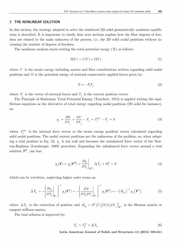
2 THE NONLINEAR SOLUTION

In this section, the strategy adopted to solve the reinforced 2D solid geometrically nonlinear equilib-

rium is described. It is important to clarify that next sections explain how the fiber degrees of free-

dom are related to the main unknown of the process, i.e., the 2D solid nodal positions without in-

creasing the number of degrees of freedom.

The nonlinear analysis starts writing the total potential energy (Π) as follows:

( ) ( ) ( )Y U Y YΠ = + Ω (1)

where U is the strain energy including matrix and fiber contributions written regarding solid nodal

positions and Ω is the potential energy of external conservative applied forces given by:

j jFYΩ = − (2)

where jF is the vector of external forces and jY is the current position vector.

The Principle of Stationary Total Potential Energy (Tauchert, 1974) is applied writing the equi-

librium equations as the derivative of total energy regarding nodal positions (2D solid for instance),

as:

int 0j j j j

j j

Ug F F F

Y Y

∂Π ∂= = − = − =∂ ∂

(3)

where intjF is the internal force vector or the strain energy gradient vector calculated regarding

solid nodal positions. The nodal current positions are the unknowns of the problem, so, when adopt-

ing a trial position in Eq. (3) jg is not null and becomes the unbalanced force vector of the New-

ton-Raphson (Luenberger, 1989) procedure. Expanding the unbalanced force vector around a trial

solution 0Y , one has:

0

2

( )

( ) ( ) 0j

j j k j

k

gg g Y O

Y

∂= + ∆ + =

∂0

Y

Y Y (4)

which can be rewritten, neglecting higher order terms as:

( ) ( )0 0

1 12

10 0 0( ) ( )j

k j j kj j

k k j

g UY g g H g

Y Y Y

− −

− ∂ ∂ ∆ = − = − = − ∂ ∂ ∂ Y Y

Y Y Y (5)

where kY∆ is the correction of position and ( ) ( ) 0

2kj k jH U Y Y= ∂ ∂ ∂

Y is the Hessian matrix or

tangent stiffness matrix.

The trial solution is improved by:

0k k kY Y Y= + ∆ (6)


Latin American Journal of Solids and Structures

until kY∆ or jg become sufficiently small

applied if one wants to describe the equilibrium path of the analyzed structure.

3 ISOPARAMETRIC 2D SOLID FINITE ELEMENT

As we are interested in composite analysis the procedure described in

continuum part of the composite, i.e., the matrix. After achieving the strain energy of the matrix

the next section is concerned with the introduction of the fiber strain energy into the mechanical

system.

3.1 Kinematical approximation and positional mapping

By means of the illustration of a quadratic finite element, Figure 1 shows the 2D solid (matrix)

mapping from the initial configuration (not deformed)

al., 2000). This mapping is done using a dimensionless auxiliary configuration

Figure 1: Initial and current configuration mappings.

The initial configuration 0B whose points have coordinates

space 1B with coordinates iξ using shape functions of any order,

of the nodes l in the initial configuration,

i i l ix f X

Similarly, the current configuration B

pression:

i i l iy f Y

Matrix contact stress analysis for elastic 2D composite solids


become sufficiently small (Luenberger, 1989). The load level can be incrementally

applied if one wants to describe the equilibrium path of the analyzed structure.

ISOPARAMETRIC 2D SOLID FINITE ELEMENT – ISOTROPIC CONTINUUM

As we are interested in composite analysis the procedure described in this section is applied to the



pproximation and positional mapping


mapping from the initial configuration (not deformed) 0B to its current configuration B (Bonet et

. This mapping is done using a dimensionless auxiliary configuration 1B .

Initial and current configuration mappings.

whose points have coordinates ix is mapped from the dimensionless

using shape functions of any order, ( )1 2,lφ ξ ξ , and by the coordinates

in the initial configuration, liX , such as:

( )01 2,

li i l ix f Xφ ξ ξ= =

B is mapped from the dimensionless space 1B by the e

( )11 2,

li i l iy f Yφ ξ ξ= =

. The load level can be incrementally

this section is applied to the




Bonet et

is mapped from the dimensionless

, and by the coordinates

(7)

by the ex-

(8)



where iy are coordinates of points in the current configuration, liY are the current node positions,

1,...,l N= are nodes and 1,2i = correspond to coordinate directions.

The deformation function f that maps the initial configuration 0B to the current configuration

B can be written as a composition of mappings 0f and 1f as:

( ) 11 0−

= f f f (9)

The deformation gradient A can be derived directly from 0A and 1A as (Bonet et al., 2000;

Coda and Paccola, 2007):

1 0 1( )−= ⋅A A A , with 0

0 iij

j

fA

ξ

∂=∂

, 1

1 iij

j

fA

ξ

∂=∂

(10)

Equation (10) can be understood as a numerical chain rule because the initial mapping gradient 0A is a known numerical quantity. The solid element has any order of approximation and N is the

number of nodes given as a function of the approximation order GP as:

( 1)( 2)

2

GP GPN

+ += (11)

3.2 Continuum strain energy

Without loss of generality, to simulate the continuum portion of the composite (matrix) we adopted

the Saint-Venant-Kirchhoff specific strain energy function (Ciarlet, 1993; Ogden, 1984), as:

1

2mat ij ijkl klu E E= C (12)

where ijklC is the elastic fourth-order tensor and E is the Green-Lagrange second-order strain ex-

pressed respectively by:

( )2

1 2ijkl ij kl ik jl il jk

GG

νδ δ δ δ δ δν

= + +−

C (13)

( ) ( )1 1

2 2ij ij ij ki kj ijE C A Aδ δ= − = − (14)

The variables ⋅tC = A A and δδδδ are the right Cauchy-Green stretch tensor and the Kroenecker

delta, respectively. In Eq. (13), G is the shear modulus and ν is the Poisson's ratio.

The strain energy accumulated in the continuum part of the composite (matrix) is calculated by

integrating the specific strain energy over the initial volume, i.e.,

0

0mat matV

U u dV= ∫ (15)



Considering solids with unitary thickness and writing Eq. (15) as a function of dimensionless

coordinates ( 1ξ and 2ξ ) results:

21 1

1 2 0 1 2 1 20 0( , ) ( , )mat matU u J d d

ξξ ξ ξ ξ ξ ξ

−= ∫ ∫ (16)

where 0J is the Jacobian of the initial mapping, i.e.,

00 1 2( , ) det( )J ξ ξ = A (17)

with 0A given by Eq. (10).

The matrix strain energy can be derived directly regarding the solid finite element positions find-

ing the conjugate internal force vector, as:

1

0

11int

0 0 1 2 2 1

0 0

( , )mat mat mat

v

U u uF dV J d d

Y Y Y

ξβ

α β β βα α α

ξ ξ ξ ξ

−∂ ∂ ∂

= = =∂ ∂ ∂∫ ∫ ∫ (18)

in which α is the direction and β is the node. The derivative inside the integral term of Eq. (18)

can be developed as:

1

: : :2

mat matu u

Y Y Yβ β βα α α

∂ ∂ ∂ ∂ ∂= =∂ ∂∂ ∂ ∂

E C CS

E C (19)

where matu∂ ∂S = E is the second Piola-Kirchhoff stress tensor. From the definition of the right

Cauchy stretch and Eq. (10) one writes:

1 1

0 1 0 1 0 1 0 1( )( ) ( ) ( ) ( ) ( )

TT T T

Y Y Yβ β βα α α

− − − −∂∂ ∂= ⋅ ⋅ ⋅ + ⋅ ⋅ ⋅

∂ ∂ ∂

AC AA A A A A A (20)

From Eq. (8) results

1

, 1 2 , 1 2 , 1 2( , ) ( , ) ( , )l

ij il j l j l i j i

A Y

Y Yβ α β αβ β

α α

φ ξ ξ φ ξ ξ δ δ φ ξ ξ δ∂ ∂

= = =∂ ∂

(21)

To complete the necessary variables of the solution process (section 2) it is necessary to calculate

the second derivative of strain energy regarding nodal positions, resulting into the Hessian matrix

as:

0

2 2

0mat mat mat

V

U uH dV

Y Y Y Yαβγξ β ξ β ξ

α γ α γ

∂ ∂= =∂ ∂ ∂ ∂∫ (22)

in which



2 2 21 1

: : :4 2

mat mat matu u u

Y Y Y Y Y Yβ ξ ξ β ξ βα γ γ α γ α

∂ ∂ ∂∂ ∂ ∂= +

∂ ∂ ∂∂ ∂ ∂ ∂ ∂ ∂

C C C

E E E (23.a)

or

2 21 1

: : :4 2

matu

Y Y Y Y Y Yβ ξ ξ β ξ βα γ γ α γ α

∂ ∂ ∂ ∂= +

∂ ∂ ∂ ∂ ∂ ∂

C C CSC (23.b)

and

2 1 12 10 1 0 1 0 0 1

1 1 2 10 0 1 0 1 0 1

( ) ( )( ) ( ) ( ) ( )

( ) ( ) ( ) ( ) ( ) ( )

T TT T

TT T T

Y Y Y Y Y Y

Y Y Y Y

β ξ β ξ β ξα γ α γ α γ

ξ β β ξγ α α γ

− − − −

− − − −

∂ ∂∂ ∂= + +

∂ ∂ ∂ ∂ ∂ ∂

∂ ∂ ∂+

∂ ∂ ∂ ∂

. . . . .

. . . . . .

A AC AA .A A A A

A A AA A A A A

(24)

It should be noted that, for solid elements, the second derivative of 1A regarding nodal parame-

ters is null, simplifying expression (24) to:

1 12 1 1

0 0 1 0 0 1( ) ( )( ) ( ) ( ) ( )

T TT T

Y Y Y Y Y Yβ ξ β ξ ξ βα γ α γ γ α

− − − −∂ ∂∂ ∂ ∂= +

∂ ∂ ∂ ∂ ∂ ∂. . . . . .

A AC A AA A A A (25)

Next section presents the necessary expressions to introduce fibers into the composite formula-

tion.

4 ELASTIC FIBER REINFORCEMENT – KINEMATICS AND ENERGY CONSIDERATIONS

This section is divided into two subsections. The first describes the strain energy of general curved

fibers and the second describes the strategy used to introduce fiber energy in the composite solution

without increasing the number of degrees of freedom.

4.1 Any order curved fiber element

To guaranty total adherent fiber-matrix coupling when using high order solid elements it is also

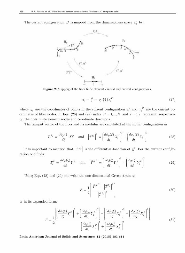
necessary to adopt high order fiber elements (Sampaio et al., 2013). Figure 2 shows the non-

deformed initial configuration 0B , the current configuration B and a non-dimensional auxiliary

configuration 1B for the curved fiber finite element of any order.

The initial configuration 0B whose points have coordinates ix is mapped from the dimensionless

space 1B with coordinates ξ using shape functions of any order, ( )Pφ ξ , and by the coordinates of

nodes P , PiX , at the initial configuration, such as:

( )0 Pi i P ix f Xφ ξ= = (26)


Latin American Journal of Solids and Structures

The current configuration B is mapped from the dimensionless space

Figure 2: Mapping of the fiber fin

i i P iy f Y

where iy are the coordinates of points in the current configuration

ordinates of fiber nodes. In Eqs. (26) and (27) index

ly, the fiber finite element nodes and coordinate directions.

The tangent vector of the fiber and its modulus are calculated at the initial configuration as

0( )B P P

i i

dT X

d

φ ξ

ξ= and

It is important to mention that 0BT

ration one finds:

( )B P P

i i

dT Y

d

φ ξ

ξ= and

Using Eqs. (28) and (29) one write the one

E =

or in its expanded form,

2 2 2 2

1 2 1 2

( ) ( ) ( ) ( )

1

2

P P P Pl l l ld d d dY Y X X

d d d dE

d d

φ ξ φ ξ φ ξ φ ξ

ξ ξ ξ ξ

+ − + =

Matrix contact stress analysis for elastic 2D composite solids


is mapped from the dimensionless space 1B by:

Mapping of the fiber finite element - initial and current configurations.

( )1 Pi i P iy f Yφ ξ= =

are the coordinates of points in the current configuration B and PiY are the current c

ordinates of fiber nodes. In Eqs. (26) and (27) index 1,...,P N= and 1,2i = represent, respectiv

ly, the fiber finite element nodes and coordinate directions.

The tangent vector of the fiber and its modulus are calculated at the initial configuration as

and 0

2 22

1 2

( ) ( )B P P P Pd dT X X

d d

φ ξ φ ξ

ξ ξ

= +

is the differential Jacobian of 0if . For the current config

and

2 22

1 2

( ) ( )B l P l Pd dT Y Y

d d

φ ξ φ ξ

ξ ξ

= +

(28) and (29) one write the one-dimensional Green strain as

0

0

22

2

1

2

BB

B

T T

T

− =

2 2 2 2

1 2 1 2

2 2

1 2

( ) ( ) ( ) ( )

( ) ( )

P P P Pl l l l

P Pl l

d d d dY Y X X

d d d d

d dX X

d d

φ ξ φ ξ φ ξ φ ξ

ξ ξ ξ ξ

φ ξ φ ξ

ξ ξ

+ − +

+

(27)

are the current co-

t, respective-

(28)

. For the current configu-

(29)

(30)

(31)



Using the Saint-Venant-Kirchhoff constitutive law one writes the specific strain energy at a

point of the fiber as:

21

( ) ( )2fu Eξ ξ = ⋅ E (32)

where E is the elastic modulus and ( )E ξ is the Green strain measure defined by Eq. (30) or (31).

The strain energy of a curved fiber is given by integrating equation (32) over its initial volume

0V as:

0

0f fV

U u dV= ∫ (33)

In order to proceed with the equilibrium analysis it is necessary to know the first derivative of

strain energy regarding positions. Based on the energy conjugate concept the natural internal fiber

force vector related to node j and direction k (intj f

kF ) is calculated regarding fiber parameters as:

0

int

0

j f f f

k j jVk k

U uF dV

Y Y

∂ ∂= =∂ ∂

∫ (34)

From Eqs. (31) and (32) follows

0 0

int

0 020

( )( ) jllk

j f f

k j V Vk

ddY

U d dF E dV E S dV

Y T

φ ξφ ξ

ξ ξ

∂ = = ⋅ = ⋅∂

∫ ∫E (35)

in which S is the one-dimensional Second Piola-Kirchhoff stress. Considering S constant over the

cross section area A of the fiber one transforms 0fdV into a simple expression, resulting:

0 1int

0 02 20 10 0

( ) ( )( ) ( )

( )

j jl ll lk k

Lj f

k

d dd dY Y

d d d dF E Ads E J Ad

T T

φ ξ φ ξφ ξ φ ξ

ξ ξ ξ ξξ ξ

−

= ⋅ = ⋅ ⋅∫ ∫E E (36)

Where, as mentioned before,

2 2

0 1 20( )

dx dxJ T

d dξ

ξ ξ

= = +

(37)

The Hessian matrix components for the fiber element are obtained by the second derivative of

the strain energy, i.e.:



0 0

2 2

0 0f f

f ff ff fkj kjj jV V

k k

U uH dV h dV

Y Y Y Yαβ αββ β

α α

∂ ∂= = =∂ ∂ ∂ ∂

∫ ∫ (38)

Developing the necessary calculations one achieves:

0

04 20 0

( ) ( ) ( ) ( )( ) ( ) j jf l l l lkj k k

V

d d d dd dE EH Y Y dV

d d d d d dT T

β β

αβ α α

φ ξ φ ξ φ ξ φ ξφ ξ φ ξδ

ξ ξ ξ ξ ξ ξ

⋅ ⋅ = + ∫

E E (39)

or

1

04 21 0 0

( ) ( ) ( ) ( )( ) ( )( )

j jf l l l lkj k k

d d d dd dE EH Y Y A J d

d d d d d dT T

β β

αβ α α

φ ξ φ ξ φ ξ φ ξφ ξ φ ξδ ξ ξ

ξ ξ ξ ξ ξ ξ−

⋅ ⋅ = + ⋅ ∫E E

(40)

Integrals (36) and (40) are solved using Gauss-Legendre quadrature.

The parameters used to find the internal force and Hessian matrix for fibers are not suitable to

be directly applied in the solid solution process; in next section the necessary transformations are

presented.

4.2 Coupling strategy – kinematical fiber matrix coupling

The procedure adopted here to embed fibers at any position of the domain without increasing the

number of degrees of freedom is an extension of the works of Vanalli et al. (2008) where linear ele-

ments and linear elasticity were adopted.

4.2.1 General fiber / solid connection

The requisite to start the procedure to embed curved fibers in curved solid elements is to know the

solid dimensionless coordinates related to fiber nodes coordinates. This is done solving the pair of

dimensionless solid variable 1 2( , )p pξ ξ associated to the physical fiber node position in the following

nonlinear system,

1 2( , )P P l Pl i iX Xφ ξ ξ = (41)

where lφ are the shape functions of the solid element, PiX are the known physical coordinates of

fiber nodes (generated independently of solid mesh) and liX are the know solid nodes coordinates.

To solve Eq. (41) one expands it in Taylor series until the first order and starts with a trial dimen-

sionless coordinate, 1 2( , )pt ptξ ξ , i.e.:

1 2

1 21 2

( , )

( , )( , )

Pt Pt

P Pt Pt l li l i j

j

X X

ξ ξ

φ ξ ξφ ξ ξ ξ

ξ

∂≅ + ∆

∂ or P Pt

i i ij jX X H ξ= + ∆ (42)



in which PtiX is a trial position of the fiber node calculated from the solid element geometry and

the trial dimensionless coordinates and ijH is a two dimensional matrix. The correction of the trial

dimensionless coordinates iξ∆ is calculated solving the following linear system of equation:

P Ptij j i iH X Xξ∆ = − (43)

The procedure is a simple and fast Newton-Raphson nonlinear solver that relates all fiber nodes

to the connected solid element revealing the pair of dimensionless variables 1 2( , )p pξ ξ . From this in-

formation one also knows the current position of fiber nodes as a function of solid nodes positions,

i.e.,

1 2( , )P P P li l iY Yφ ξ ξ= (44)

in which liY are the current positions of solid nodes. Equation (44) ensures the connection among

nodes of fibers and the matrix 2D elements.

In the next item it will be necessary to differentiate the fiber strain energy regarding the solid

nodal coordinates using the chain rule. To make it possible one has to differentiate Eq. (44) regar-

ding a generic nodal solid coordinate, as:

1 2 1 2( , ) ( , )P li i P P P P

l i l l

Y Y

Y Yα ββ β

α α

φ ξ ξ δ δ φ ξ ξ∂ ∂

= =∂ ∂

(45)

If the fiber node P belongs to the solid element then 1lβδ = and if direction α (solid) is equal

to direction i (fiber) then 1iαδ = and expression (45) results 1 2( , )P P PiY Y βα βφ ξ ξ∂ ∂ = , otherwise it

results zero.

4.2.2 General internal force

The strain energy stored in a reinforced body is the sum of the strain energies stored in the matrix

and fibers,

mat fU U U= + (46)

where matU is the strain energy stored in the 2D solid finite elements used to discretize the matrix

and fU is the strain energy stored in the fiber finite elements. Therefore, the internal force at a

node β following direction α , considering both fiber and matrix contributions is found by the con-

jugate energy concept, such as:

int

1 2

( )( , )

Pmat P fmat f f fmat mat i P P

Pi

U U U UU U YF F F

Y Y Y Y Y Y

β β

α β α αβ β β β βα α α α α

φ ξ ξ∂ + ∂ ∂∂ ∂ ∂

= + = + = + =∂ ∂ ∂ ∂ ∂ ∂

(47)

where Eqs. (18), (36) and (45) have been used and there is no summation over P .



4.2.3 Hessian Matrix

Proceeding as described for the calculation of internal forces, we develop the second derivative of

strain energy of the reinforced finite element regarding the solid nodal parameters, as follows

( )

0 0 0

2 2 222

0 0 0

( )

f

mat f mat f fmat f

V V V

U U u u uuUdV dV dV

Y Y Y Y Y Y Y Y Y Yβ ξ β ξ β ξ β ξ β ξα γ α γ α γ α γ α γ

∂ + ∂ + ∂∂∂= = = +

∂ ∂ ∂ ∂ ∂ ∂ ∂ ∂ ∂ ∂∫ ∫ ∫ (48)

The first integral at the last term of Eq. (48) is known, Eq. (22). However, it is necessary to

observe that the kernel of the last integral is the specific strain energy of a fiber derived twice re-

garding the solid nodal parameters. As Eq. (39) gives its value when derived regarding fiber para-

meters one has to apply the chain rule twice, described by Eq. (45), over Eq. (48), that is:

2 2 2 2 2f f f f f f f f

f f f f f

f f f f f f f fw

u u u u uY Y Y Y Y Y Y Y

Y Y Y Y Y Y Y Y Y Y Y Y Y Y Y Y Y Y

ρ ρ ρ η η ρ η ηω ω ω π π ω π π

β ξ ρ ρ β ξ ρ η β ξ η ρ β ξ η η β ξα γ ω α γ ω π α γ π ω α γ π π α γ

∂ ∂ ∂ ∂ ∂∂ ∂ ∂ ∂ ∂ ∂ ∂ ∂= + + +

∂ ∂ ∂ ∂ ∂ ∂ ∂ ∂ ∂ ∂ ∂ ∂ ∂ ∂ ∂ ∂ ∂ ∂ (49)

2 f f f f f f f f

f f f f fu Y Y Y Y Y Y Y Y

h h h hY Y Y Y Y Y Y Y Y Y


ωρωρ ωρπη πηωρ πηπηβ ξ β ξ β ξ β ξ β ξα γ α γ α γ α γ α γ

∂ ∂ ∂ ∂ ∂ ∂ ∂ ∂ ∂= + + +

∂ ∂ ∂ ∂ ∂ ∂ ∂ ∂ ∂ ∂ (50)

where fh is the fiber Hessian matrix kernel, Eq. (38). In Eq. (50) summation is not implyied.

Integrating (50) over fiber volume gives:

2 f f f f f f f f

f f f f fU Y Y Y Y Y Y Y Y

H H H HY Y Y Y Y Y Y Y Y Y


ωρωρ ωρπη πηωρ πηπηβ ξ β ξ β ξ β ξ β ξα γ α γ α γ α γ α γ

∂ ∂ ∂ ∂ ∂ ∂ ∂ ∂ ∂= + + +

∂ ∂ ∂ ∂ ∂ ∂ ∂ ∂ ∂ ∂ (51)

Using Eq. (51) into (48) results the consistent spreading of fibers contribution over the matrix

properties, i.e.:

ef fH H H= + (52)

5 CONTACT STRESS CALCULATION

In the proposed formulation the contact stresses are not used to achieve the equilibrium position.

Therefore, the contact stress calculation is done after solving the problem for positions. Two strate-

gies are presented in order to do this calculation. The first is based on differential relations and is

presented in subsections 5.1 and 5.2. The second is an average calculation, shown at subsection 5.3,

for which the transferred nodal force from fiber to matrix is decomposed following the tangential

and normal directions of fiber node and divided by a influence portion of the element contact area.

5.1 Shear contact stress – differential formulation

The differential equilibrium depicted in Figure 3 is used to calculate the contact shear stress ( )q ξ

between fiber and matrix as:



Figure 3: Differential equilibrium following fiber direction.

1

. .dN dN

q t ds dN ds qds t ds

= = ⇒ = (53)

where ds is a differential of the curvilinear coordinate along the deformed fiber and t is the fiber

thickness. ds is calculated as a function of dimensionless coordinate ξ as:

2 2

2 2 1 21 2 ( ).

dy dyds dy dy d d J d

d dξ ξ ξ ξ

ξ ξ

= + = + = (54)

or

( )ds

Jd

ξξ= (55)

Using the chain rule results:

1 1

. .( )

dN dN d dN dN

ds d ds d ds J d

d

ξ

ξ ξ ξ ξ

ξ

= = = (56)

Considering constant thickness the Cauchy stress is calculated from Piola Kirchhoff stress as:

0 0

( ) ( )( ) ( ) ( )

( ) ( )

J JS E

J J

ξ ξσ ξ ξ ξ

ξ ξ= = E. (57)

0

( )( ) ( ).

( )

JN E A

J

ξξ ξ

ξ= E. (58)

With ( )E ξ given by equation (31).

Instead of differentiate expression (58) regarding ξ and substituting into (56) and (53) we prefer

to calculate the normal force nodal values using (31) and (58) and make:

( ) ( ) PPN Nξ φ ξ= (59)

therefore:

( )

( )p p

ddNN

d d

φ ξξ

ξ ξ= (60)



Substituting (60) into (56) and (56) into (53) results:

( )1 1

( )( )

p pd

q Nt J d

φ ξξ

ξ ξ= (61)

It is important to mention that the differential formulation cannot be applied for linear fiber

element, as it results null values of ( )q ξ .

5.2 Normal contact stress – differential formulation

For an infinitesimal length ds there is a curvature center and a curvature radius, see Figure 4.

From this figure one writes the following geometrical relation:

.ds Rdθ= (62)

Figure 4: Infinitesimal part of a fiber finite element.

Remembering that t is the body thickness, the equilibrium equation following the fiber orthogonal

direction is given by:

. . . .( . ) 2. . .2

dp t ds p t Rd N sen N d

θθ θ

= = = (63)

or

( )1

( )( )

Np

t R

ξξ

ξ= (64)

As ( )N ξ is known, equation (58), it is necessary to calculate 1 ( )R ξ , given by:

( )

2 22 1 1 2

2 2

3

1

( ) ( )

d y dy d y dy

d dd d

R J

ξ ξξ ξ

ξ ξ

−

= (65)

Substituting (65) into (64) results the final expression:



( )

2 22 1 1 2

2 2

3

1( ) ( )

( )

d y dy d y dy

d dd dp N

t J

ξ ξξ ξξ ξ

ξ

−

= (66)

By the same reason described in the previous item, expression (66) cannot be applied for linear

fiber elements. In section 6 examples are used to demonstrate the use of presented expressions.

5.3 Average contact stress

A generic nodal transfer force (from matrix to fiber) intF

is depicted in Figure 5 together with the

tangential and normal unit vectors (n and t

) calculated at the same point. The tangential and

normal components of the transfer force are:

intQ = F t⋅

(67)

intP = F n⋅

(68)

Figure 5: Transfer force and area of influence.

The normal and tangential forces are divided by the surface influence area ( infA ) depicted in Figure

5 and the average values results:

intinf

q = F t A⋅

(69)

intinf

p = F n A⋅

(70)

It is worth noting that for connecting nodes the resulting value is the average between values calcu-

lated for each element.

6 NUMERICAL EXAMPLES

Five numerical examples are chosen to show the behavior of the proposed formulation regarding the

overall behavior of reinforced structural members and the estimated contact stress accuracy. A con-

vergence analysis is carried out for both displacement and contact stresses.

6.1 Simple supported beam

This example is used to certify that the mechanical coupling between fiber and matrix is working



properly. Both displacement and contact stress are compared to a simple analytical solution limited

to small displacements and strains in order to certify the coherence of results.

It is a simple supported reinforced beam, depicted in Figure 6, subjected to a uniformly distrib-

uted load 10 N cmq = . The simple supports are modeled by vertical distributed loads of

100 N/cmrq = and the adopted geometrical properties are: 400 cmL = , 20 cmh = , 1 cmb =

and 1 cmd = , see Figure 6. The Young modulus and the Poisson´s ratio of the matrix are 5 221x10 N cmcE = and 0ν = , while the Young modulus and the cross-sectional area of the rein-

forcement are 5 2210x10 N cmfE = and 21 cmfA = . Due to symmetry, only a half of the problem

is solved as depicted by Figure 6.

Figure 6: Geometry and boundary conditions.

In order to check displacement convergence, see Figure 7, we use 160 linear fiber elements to discre-

tize the horizontal reinforcement and three different meshes of triangular third order finite elements,

i.e., mesh (a) 8x80 elements and 12050 dof, (b) 16x160 elements and 47138 dof and (c) 32x320

elements and 186434 dof. As one can see the displacement difference from the second to the third

discretization is less than 0.3% characterizing convergence. Adopting the mid position of reaction

as the span position one achieves the technical reference value ( )4 384 1.105 cmq EI⋅ =ℓ obviously

smaller than the achieved numerical value.

Figure 7: Displacement convergence.

0 50000 100000 150000 200000

-1.1699

-1.1698

-1.1697

-1.1696

Vertical displacement (cm)

Degrees of freedom (dof)

200 cm 20 cm

20 cm

100 N/cm

10 N/cm

1 cm

1 cm

19 cm

1 cm

reinforcement

x

y



The convergence analysis for shear contact stress is made using linear fibers and the average tech-

nique, see Figure 8. We adopt 80 and 160 linear fibers for meshes (a), (b) and (c). As one can see

there is no significant difference in results characterizing convergence. However, it is important to

note that when one increases the number of fiber finite elements it is also necessary to increase the

continuum mesh.

Figure 8: Contact shear stress behavior.

Adopting the average calculation formulation and using mesh (b), Figure 9 compares the shear con-

tact stress for equally spaced nodes using 160 linear, 80 quadratic and 53 third order fiber approxi-

mations. Figure 10 shows the same results of Figure 9 when the differential procedure is adopted to

calculate the shear stress for second and third order approximations (remembering that the differen-

tial procedure is not applied for first order approximation).

Figure 9: Contact shear stress for high order elements (average calculation).

From Figures 9 and 10 one concludes that when using high order fiber elements a perturbation

of the shear contact stress appears; moreover the use of differential formulation, expected to be the

0 50 100 150 200

-100

-80

-60

-40

-20

0

Contact Shear stress

Position (cm)

Technical solution

Mesh (a) - 80 Fibers

Mesh (b) - 80 Fibers

Mesh (b) - 160 Fibers

Mesh (c) - 80 Fibers

Mesh (c) - 160 Fibers



most precise one, introduces even more oscillations. At the beginning we did not know why this

spurious behavior appears, however after thinking over the subject we conclude that, due to the

nodal characteristic of internal force transfer from matrix to fibers a not recommended finite ele-

ment operation is taking place.

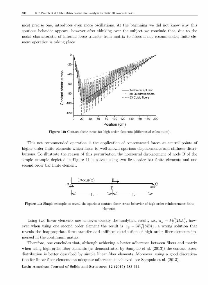
Figure 10: Contact shear stress for high order elements (differential calculation).

This not recommended operation is the application of concentrated forces at central points of

higher order finite elements which leads to well-known spurious displacements and stiffness distri-

butions. To illustrate the reason of this perturbation the horizontal displacement of node B of the

simple example depicted in Figure 11 is solved using two first order bar finite elements and one

second order bar finite element.

Figure 11: Simple example to reveal the spurious contact shear stress behavior of high order reinforcement finite

elements.

Using two linear elements one achieves exactly the analytical result, i.e., ( )2Bu Fl EA= , how-

ever when using one second order element the result is ( )3 8Bu Fl EA= , a wrong solution that

reveals the inappropriate force transfer and stiffness distribution of high order fiber elements im-

mersed in the continuum matrix.

Therefore, one concludes that, although achieving a better adherence between fibers and matrix

when using high order fiber elements (as demonstrated by Sampaio et al. (2013)) the contact stress

distribution is better described by simple linear fiber elements. Moreover, using a good discretiza-

tion for linear fiber elements an adequate adherence is achieved, see Sampaio et al. (2013).

0 20 40 60 80 100 120 140 160 180 200

-120

-100

-80

-60

-40

-20

0

Contact shear stress

Position (cm)

Technical solution

80 Quadratic fibers

53 Cubic fibers

L L

A C B

F x,u(x)



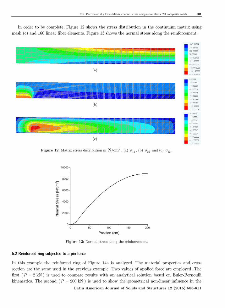
In order to be complete, Figure 12 shows the stress distribution in the continuum matrix using

mesh (c) and 160 linear fiber elements. Figure 13 shows the normal stress along the reinforcement.

(a)

(b)

(c)

Figure 12: Matrix stress distribution in 2N/cm , (a) 11σ , (b) 22σ and (c) 12σ .

Figure 13: Normal stress along the reinforcement.

6.2 Reinforced ring subjected to a pin force

In this example the reinforced ring of Figure 14a is analyzed. The material properties and cross

section are the same used in the previous example. Two values of applied force are employed. The

first ( 2 kNP = ) is used to compare results with an analytical solution based on Euler-Bernoulli

kinematics. The second ( 200 kNP = ) is used to show the geometrical non-linear influence in the

0 50 100 150 200

0

2000

4000

6000

8000

10000

Normal Stress (N/cm2)

Position (cm)



developed contact stress. Due to symmetry only a half of the problem is discretized, as depicted in

Figure 14b. The adopted matrix mesh ( 8x240 ) is chosen after a convergence analysis.

Figure 14: Geometry and matrix discretization.

For 2kNP = Figure 15 compares the analytical shear stress and the ones achieved using the

average technique for 240 and 120 linear fiber elements. Obviously that the analytical solution is

only a reference value as the Euler-Bernoulli hypothesis excessively simplifies the problem. In Figure

16 one finds the same result using 240 quadratic and 480 cubic elements, revealing the same spuri-

ous behavior detected in the previous example for high order elements. Figure 17 shows the normal

contact stress for the same load level using linear fiber elements. As expected the normal contact

stress increases near the loaded region.

Figure 15: Contact shear stress distribution – Linear elements.

0.0 0.5 1.0 1.5 2.0 2.5 3.0 3.5

-60

-40

-20

0

20

40

60

Reference

120

240

Contact shear stress (N/cm2)

Position (rad)



Figure 16: Contact shear stress distribution – High order elements.

Figure 17: Contact normal stress distribution – Linear elements.

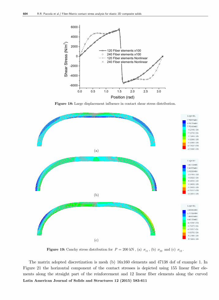
In Figure 18 we multiply by 100 the result of Figure 15 and compare it to the shear contact

stress achieved when effectively using 200 kNP = . This procedure indicates the influence of large

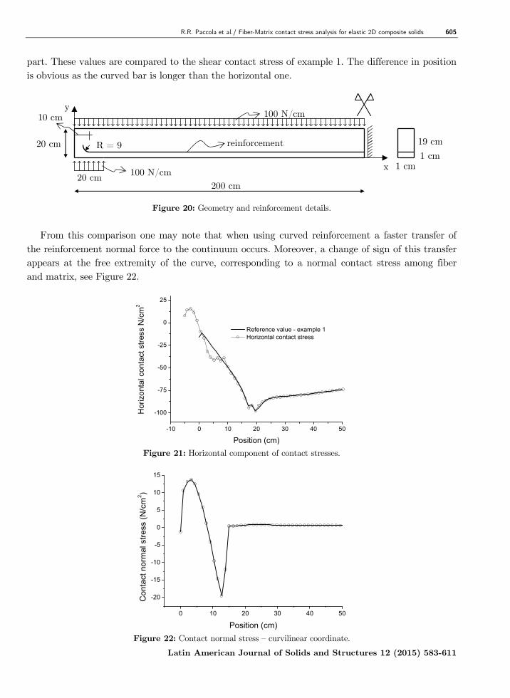
displacements in results. Figure 19 shows the deformed configuration for 200 kNP = with the

Cauchy stress distribution inside the matrix.

6.3 Curved reinforcement

In this example the same beam modeled in example 1 is solved considering the curved reinforcement

as depicted in Figure 20.

0.0 0.2 0.4 0.6 0.8 1.0 1.2 1.4

-40

-30

-20

-10

0

10

20

30

40

50

60

70

80

Reference

240 Quadratic

480 Cubic

Shear contact stress (N/cm2)

Position (rad)

0.0 0.5 1.0 1.5 2.0 2.5 3.0

-20

-10

0

10

20

30

Normal stress (N/m

2)

Position (rad)

120 Fiber Elements

240 Fiber Elements



Figure 18: Large displacement influence in contact shear stress distribution.

(a)

(b)

(c)

Figure 19: Cauchy stress distribution for 200 kNP = , (a) 11σ , (b) 22σ and (c) 12σ .

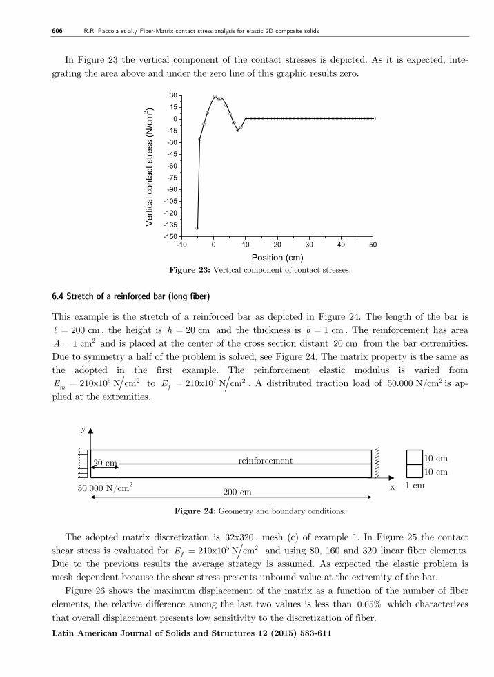
The matrix adopted discretization is mesh (b) 16x160 elements and 47138 dof of example 1. In

Figure 21 the horizontal component of the contact stresses is depicted using 155 linear fiber ele-

ments along the straight part of the reinforcement and 12 linear fiber elements along the curved

0.0 0.5 1.0 1.5 2.0 2.5 3.0

-6000

-4000

-2000

0

2000

4000

6000

Shear Stress (N/m

2)

Position (rad)

120 Fiber elements x100

240 Fiber elements x100

120 Fiber elements Nonlinear

240 Fiber elements Nonlinear



part. These values are compared to the shear contact stress of example 1. The difference in position

is obvious as the curved bar is longer than the horizontal one.

Figure 20: Geometry and reinforcement details.

From this comparison one may note that when using curved reinforcement a faster transfer of

the reinforcement normal force to the continuum occurs. Moreover, a change of sign of this transfer

appears at the free extremity of the curve, corresponding to a normal contact stress among fiber

and matrix, see Figure 22.

Figure 21: Horizontal component of contact stresses.

Figure 22: Contact normal stress – curvilinear coordinate.

-10 0 10 20 30 40 50

-100

-75

-50

-25

0

25

Horizontal contact stress N/cm2

Position (cm)

Reference value - example 1

Horizontal contact stress

0 10 20 30 40 50

-20

-15

-10

-5

0

5

10

15

Contact normal stress (N/cm2)

Position (cm)

200 cm 20 cm

20 cm

100 N/cm

100 N/cm

1 cm

19 cm

1 cm

reinforcement

x

y

R = 9

10 cm



In Figure 23 the vertical component of the contact stresses is depicted. As it is expected, inte-

grating the area above and under the zero line of this graphic results zero.

Figure 23: Vertical component of contact stresses.

6.4 Stretch of a reinforced bar (long fiber)

This example is the stretch of a reinforced bar as depicted in Figure 24. The length of the bar is

200 cm=ℓ , the height is 20 cmh = and the thickness is 1 cmb = . The reinforcement has area 21 cmA = and is placed at the center of the cross section distant 20 cm from the bar extremities.

Due to symmetry a half of the problem is solved, see Figure 24. The matrix property is the same as

the adopted in the first example. The reinforcement elastic modulus is varied from 5 2210x10 N cmmE = to 7 2210x10 N cmfE = . A distributed traction load of 250.000 N/cm is ap-

plied at the extremities.

Figure 24: Geometry and boundary conditions.

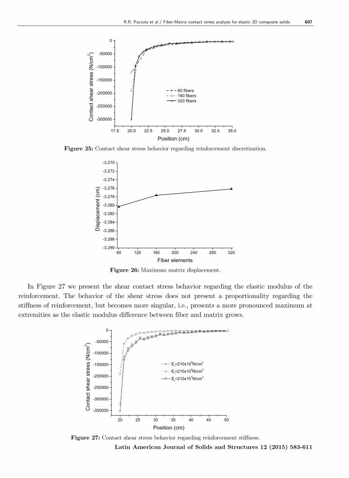
The adopted matrix discretization is 32x320 , mesh (c) of example 1. In Figure 25 the contact

shear stress is evaluated for 5 2210x10 N cmfE = and using 80, 160 and 320 linear fiber elements.

Due to the previous results the average strategy is assumed. As expected the elastic problem is

mesh dependent because the shear stress presents unbound value at the extremity of the bar.

Figure 26 shows the maximum displacement of the matrix as a function of the number of fiber

elements, the relative difference among the last two values is less than 0.05% which characterizes

that overall displacement presents low sensitivity to the discretization of fiber.

-10 0 10 20 30 40 50-150

-135

-120

-105

-90

-75

-60

-45

-30

-15

0

15

30

Vertical contact stress (N/cm2)

Position (cm)

200 cm

20 cm

50.000 N/cm2 1 cm

10 cm reinforcement

x

y

10 cm



Figure 25: Contact shear stress behavior regarding reinforcement discretization.

Figure 26: Maximum matrix displacement.

In Figure 27 we present the shear contact stress behavior regarding the elastic modulus of the

reinforcement. The behavior of the shear stress does not present a proportionality regarding the

stiffness of reinforcement, but becomes more singular, i.e., presents a more pronounced maximum at

extremities as the elastic modulus difference between fiber and matrix grows.

Figure 27: Contact shear stress behavior regarding reinforcement stiffness.

17.5 20.0 22.5 25.0 27.5 30.0 32.5 35.0

-300000

-250000

-200000

-150000

-100000

-50000

0


Position (cm)

80 fibers

160 fibers

320 fibers

80 120 160 200 240 280 320

-3.290

-3.288

-3.286

-3.284

-3.282

-3.280

-3.278

-3.276

-3.274

-3.272

-3.270

Displacement (cm)

Fiber elements

20 25 30 35 40 45 50

-350000

-300000

-250000

-200000

-150000

-100000

-50000

0


Position (cm)

Ef=210x10

5N/cm

2

Ef=210x10

6N/cm

2

Ef=210x10

7N/cm

2



Figure 28 illustrates the reinforcement influence on the matrix 11σ stress behavior. Almost all

stress is transferred to the bar along less than 25 cm. It is important to mention that the limits

adopted in legend of Figure 28 are taken on purpose to show the transition that is hidden if the

total stress range is assumed.

Figure 28: Matrix horizontal stress behavior ( 7 2210x10 N/cmfE = ).

6.5 Stretch of a reinforced bar (short random fibers)

The same bar of example 6.5 is reinforced by 4000 random short fibers instead of a single long fiber.

Short fibers are 5cm long and have a cross section area of 20.1 cm . Three values of elastic modulus

are adopted: 6 2210x10 N cmfE = , 7 2210x10 N cmfE = and 8 2210x10 N cmfE = . The random

fibers and the matrix discretization are depicted in Figure 29.

Figure 29: Random fibers and matrix discretization.

The matrix horizontal stress distributions for different fiber elastic modulus are presented in

Figure 30. The same maximum and minimum values have been adopted to facilitate comparisons.

6 2210x10 N cm

fE =

7 2210x10 N cm

fE =

8 2210x10 N cm

fE =

Figure 30: Matrix stress ( 11σ ) distribution – same scale - 2N/cm .



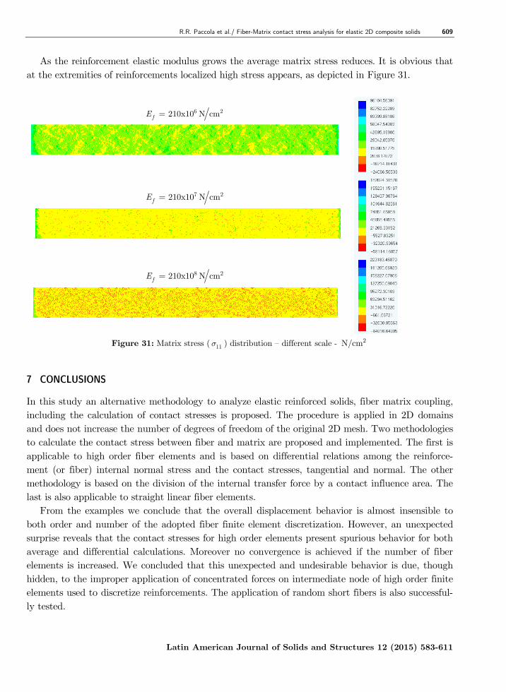
As the reinforcement elastic modulus grows the average matrix stress reduces. It is obvious that

at the extremities of reinforcements localized high stress appears, as depicted in Figure 31.

6 2210x10 N cmfE =

7 2210x10 N cmf

E =

8 2210x10 N cmf

E =

Figure 31: Matrix stress ( 11σ ) distribution – different scale - 2N/cm

7 CONCLUSIONS

In this study an alternative methodology to analyze elastic reinforced solids, fiber matrix coupling,

including the calculation of contact stresses is proposed. The procedure is applied in 2D domains

and does not increase the number of degrees of freedom of the original 2D mesh. Two methodologies

to calculate the contact stress between fiber and matrix are proposed and implemented. The first is

applicable to high order fiber elements and is based on differential relations among the reinforce-

ment (or fiber) internal normal stress and the contact stresses, tangential and normal. The other

methodology is based on the division of the internal transfer force by a contact influence area. The

last is also applicable to straight linear fiber elements.

From the examples we conclude that the overall displacement behavior is almost insensible to

both order and number of the adopted fiber finite element discretization. However, an unexpected

surprise reveals that the contact stresses for high order elements present spurious behavior for both

average and differential calculations. Moreover no convergence is achieved if the number of fiber

elements is increased. We concluded that this unexpected and undesirable behavior is due, though

hidden, to the improper application of concentrated forces on intermediate node of high order finite

elements used to discretize reinforcements. The application of random short fibers is also successful-

ly tested.



In future works we intend to apply the successful developments of this paper to consider slip

among fiber and matrix without increasing the number of degrees of freedom.

Acknowledgements

This research is supported by the Coordenação de Aperfeiçoamento de Pessoal de Nível Superior

(CAPES), Amazon Research Foundation (FAPEAM) and São Paulo Research Foundation

(FAPESP).

References

Babuska, I., Melenk, J.M., (1997). The partition of unity method. International Journal for Numerical Methods in

Engineering 40: 727–758.

Balakrishnan, S., Murray, D.W., (1986). Finite element prediction of reinforced concrete. Ph.D. Thesis, University of

Alberta.

Bolander Jr, J.E., Saito, S., (1997). Discrete modeling of short-fiber reinforcement in cementitious composites. Ad-

vanced Cement Based Materials 6: 76–86.

Bonet, J., Wood, R.D., Mahaney, J., Heywood, P., (2000). Finite element analysis of air supported membrane struc-

tures. Computer Methods in Applied Mechanics and Engineering 5-7: 579-595.

Ciarlet, P. G., (1993). Mathematical Elasticity. North-Holland.

Chudoba, R., Jerábek, J., Peiffer, F., (2009). Crack-centered enrichment for debonding in two-phase composite ap-

plied to textile reinforced concrete. International Journal for Multiscale Computational Engineering 7(4): 309–328.

Coda, H. B., (2001). Dynamic and static non-linear analysis of reinforced media: a BEM/FEM coupling approach.

Computers & Structures, 79(31): 2751-2765.

Coda, H.B., (2009). A solid-like FEM for geometrically non-linear 3D frames, Computer methods in applied mechan-

ics and engineering 198(47-48): 3712-3722.

Coda, H.B., Paccola, R.R., (2007). An alternative positional FEM formulation for geometrically nonlinear analysis of

shells: Curved triangular isoparametric elements. Computational Mechanics 40(1): 185-200.

Coda, H.B., Paccola, R.R, (2008). A positional FEM Formulation for geometrical non-linear analysis of shells, Latin

American Journal of Solids and Structures 5(3): 205-223.

Désir, J.-M., Romdhane, M.R.B., Ulm, F.-J., Fairbairn, E.M.R., (1999). Steel–concrete interface: revisiting constitu-

tive and numerical modeling. Computers and Structures 71: 489–503.

Duarte, C.A., Babuska, I., Oden, J.T., (2000). Generalized finite element methods for three-dimensional structural

mechanics problems. Computers and Structures 77: 215–232.

Duarte, C.A., Oden, J.T., (1996a). H-p clouds-an h-p meshless method. Numerical Methods for Partial Differential

Equations 12: 673–705.

Duarte C.A., Oden, J.T., (1996b). An h-p adaptive method using clouds. Computer Methods in Applied Mechanics

and Engineering 139: 237–262.

Hettich, T., Hund, A., Ramm, E., (2008). Modeling of failure in composites by X-FEM and level sets within a

multiscale framework. Computer Methods in Applied Mechanics and Engineering 197: 414-424.

Leite, L.G.S., Venturini, W.S., Coda, H.B., (2003). Two dimensional solids reinforced by thin bars using the bounda-

ry element method. Engineering Analysis with Boundary Elements 3(27): 193-201.

Li, Z., Perez Lara, M.A., Bolander, J.E., (2006). Restraining effects of fibers during non-uniform drying of cement

composites. Cement and Concrete Research 36: 1643–1652.

Luenberger, D. G., (1989). Linear and nonlinear programming. Addison-Wesley Publishing Company.



Melenk, J.M., Babuska, I., (2006). The partition of unity finite element method: basic theory and applications. Com-

puter Methods in Applied Mechanics and Engineering 139: 289–314.

Oden, J.T., Duarte, C.A.M., Zienkiewicz, O.C., (1998). A new cloud-based hp finite element method. Computer

Methods in Applied Mechanics and Engineering 153: 117–126.

Ogden, R.W., (1984). Nonlinear Elastic deformation, Ellis Horwood, England.

Oliver, J., Linero, D.L., Huespe, A.E., Manzoli, O.L., (2008). Two-dimensional modeling of material failure in rein-

forced concrete by means of a continuum strong discontinuity approach. Computer Methods in Applied Mechanics

and Engineering 197: 332–348.

Pascon, J.P., Coda, H.B., (2013). A shell finite element formulation to analyze highly deformable rubber-like materi-

als. Latin American Journal of Solids and Structures 10: 1177-1209.

Radtke, F.K.F., Simone, A., Sluys, L.J., (2010a). A partition of unity finite element method for obtaining elastic

properties of continua with embedded thin fibres, International Journal for Numerical Methods in Engineering 84

(6): 708-732.

Radtke, F.K.F., Simone, A., Sluys, L.J., (2010b). A computational model for failure analysis of fibre reinforced con-

crete with discrete treatment of fibres. Engineering Fracture Mechanics 77(4): 597-620.

Radtke, F.K.F., Simone, A., Sluys, L.J., (2011). A partition of unity finite element method for simulating nonlinear

debonding and matrix failure in thin fibre composites. International Journal for Numerical Methods in Engineering

86(4-5): 453-476.

Sampaio, M.S.M., Paccola, R.R., Coda, H.B., (2013). Fully adherent fiber-matrix FEM formulation for geometrically

nonlinear 2D solid analysis. Finite Elements Analysis and Design 66: 12-25.

Schlangen, E., Van Mier, J.G.M., (1992). Simple lattice model for numerical simulation of fracture of concrete mate-

rials and structures. Materials and Structures 25: 534–542.

Tauchert, T.R., (1974). Energy principles in structural mechanics. McGraw Hill.

Vanalli, L., Paccola, R.R., Coda, H.B., (2008). A simple way to introduce fibers into FEM models. Communication

in numerical methods in Engineering 24: 585-603.

Fiber-matrix Contact Stress Analysis for Elastic 2D ... · Three widely used composite materials...

Documents

Transcript of Fiber-matrix Contact Stress Analysis for Elastic 2D ... · Three widely used composite materials...