Federal Reserve Bank of New York

Staff Reports

Quantifying the Benefits of a Liquidity-Saving Mechanism

Enghin Atalay

Antoine Martin

James McAndrews

Staff Report no. 447

May 2010

This paper presents preliminary findings and is being distributed to economists

and other interested readers solely to stimulate discussion and elicit comments.

The views expressed in this paper are those of the authors and are not necessarily

reflective of views the Federal Reserve Bank of New York or the Federal Reserve

System. Any errors or omissions are the responsibility of the authors.

Quantifying the Benefits of a Liquidity-Saving Mechanism

Enghin Atalay, Antoine Martin, and James McAndrews

Federal Reserve Bank of New York Staff Reports, no. 447

May 2010

JEL classification: E42, E58, G21

Abstract

This paper attempts to quantify the benefits associated with operating a liquidity-saving

mechanism (LSM) in Fedwire, the large-value payment system of the Federal Reserve.

Calibrating the model of Martin and McAndrews (2008), we find that potential gains are

large compared to the likely cost of implementing an LSM, on the order of hundreds of

thousands of dollars per day.

Key words: liquidity-saving mechanisms, real-time gross settlement, large-value payment

systems

Atalay: Ph.D. candidate, University of Chicago (e-mail: atalay@uchicago.edu). Martin: Federal

Reserve Bank of New York (e-mail: antoine.martin@ny.frb.org). McAndrews: Federal Reserve

Bank of New York (e-mail: jamie.mcandrews@ny.frb.org). The authors thank Marco Galbiati,

Thor Koeppl, Tomohiro Ota, Jean-Charles Rochet, Matthew Willison, and seminar participants at

the University of Western Ontario, the University of Mannheim, the Higher School of Economics,

the Bank of England, Banque de France, the Moncasca Workshop (Rome 2008), and the

Payments and Networks Conference (Santa Barbara 2008) for useful comments, as well as

Jeffrey Shrader for excellent research assistance. The views expressed in this paper are those of

the authors and do not necessarily reflect the position of the Federal Reserve Bank of New York

or the Federal Reserve System.

1 Introduction

This paper attempts to quantify the benefits from operating a liquidity-saving mechanism

(LSM) on a real-time gross settlement (RTGS) large-value payment system. Using data from

Fedwire, the large-value payment system of the Federal Reserve, we find that these gains

are large compared to the likely cost of implementing an LSM, on the order of hundreds of

thousands of dollars per day. Our paper is the first attempt to use data from the payment

system operated by a large central bank to estimate the benefits of an LSM.

LSMs are queuing arrangements that operate in conjunction with an interbank settle-

ment system. Queued payments are released when some prespecified rule has been satisfied.

Typically, a payment is released from the queue if the sending bank’s balance is above some

minimum threshold or if the payment is part of a multilaterally offsetting group of payments.

TARGET 2, the large-value payment system used in the euro area, already includes an LSM.

The Bank of Japan introduced an LSM in October 2008. The Federal Reserve is studying

the benefits and costs of implementing an LSM for Fedwire, its large-value payment system.

Hence, evaluating the performance of different LSM designs is an important policy issue.

We calibrate the model of Martin and McAndrews (2008) to quantify the improvement

that could be achieved by including a liquidity-saving mechanism in Fedwire. In the model,

banks choose whether to make a payment early or late in the day. Sending a payment early

increases the risk of incurring an overdraft fee from the central bank. Delaying a payment

can be costly because it negatively affects the banks’customers or counterparties.

The difference between the expected cost of sending a payment early and the expected

cost of delaying a payment is increasing in the fraction of other banks that delay their pay-

ments. Without an LSM, this strategic complementarity creates the possibility of multiple

equilibria, including an equilibrium where all banks decide to delay their payments.

We use Fedwire data to calibrate the model. Our data suggest that the size of liquidity

shocks on Fedwire is relatively small. The benefits of an LSM are large in that region of

the parameter space. Hence our calibration suggests that implementing an LSM for Fedwire

would have important benefits. Indeed, we find that the benefits of implementing a liquidity-

saving mechanism are over $500, 000 per day, in some cases considerably more.

The remainder of the paper proceeds as follows. Section 2 reviews Martin andMcAndrews

1

(2008) and Atalay et al. (2010). Section 3 describes our calibration and section 4 offers a

brief conclusion.

2 Model Set-up and Results

In this section, we review the main results of Martin and McAndrews (2008). Section 2.1

describes the model and defines the parameters that will be calibrated in section 3. Section

2.2 presents the equilibrium and the socially optimal allocations for the case without an

LSM and alternatively when a liquidity-saving mechanism is available. For a more detailed

discussion, see Martin and McAndrews (2008) or Atalay et al. (2010).

2.1 Set-up

The model lasts two periods, morning and afternoon. There is a unit mass of banks of equal

size. Each bank must make and receive one payment during the day. A fraction θ ∈ [0, 1]

of the banks must make a time-critical payment. Banks that delay time-critical payments

incur a cost γ > 0. The remaining 1 − θ banks have a non-time-critical payment that can

be delayed at no cost.

Before the beginning of the morning period, banks face a shock to their balances with

the central bank. We can think of this liquidity shock as a payment that must be made

in the morning and won’t be offset until the afternoon. A fraction σ ∈ [0, 14] of the banks

receive a negative liquidity shock of size 1−µ ∈ [0, 12]; a fraction σ receive a positive liquidity

shock of size 1 − µ; and the remaining 1 − 2σ banks do not receive a liquidity shock. So,

banks can be one of six types. They can have a positive, a negative, or no liquidity shock.

Furthermore, independent of the liquidity shock, banks can have a time-critical payment or

a payment that can be delayed without cost.

Banks that have a negative balance at the end of the morning period must pay an

overdraft fee R > 0 on their balances. Banks with a positive position do not earn any

interest on their balances and cannot loan their excess funds to other banks.1 Banks decide

whether to delay or send their payments early by comparing the expected costs of each

1There is no market for intraday reserves. See Martin and McAndrews (2010) for a discussion.

2

Nature chooseswhich banks receivea liquidity shock anda time­sensitivepayment

Morning period

Banks decidewhether to sendpayments in themorning, to delay, orto queue (if available)

Borrowing costsincurred if balance isnegative, delay costsif time­criticalpayment not made

Afternoon period

All remainingpayments made

Figure 1: Timeline for shocks and for sending and receiving payments.

option, while forming rational expectations about the probability of receiving a payment in

the morning.

If an LSM is present, banks have a third option. They can choose to send their payments

to a queue, which will release the payment provided that doing so does not cause the bank

to incur an overdraft. The number of payments that are released from the queue depends on

the underlying pattern of payments. For this paper, we assume that the payments form one

cycle (i.e., bank A’s payment is destined for bank B, bank B’s payment is for bank C, ....,

bank Y ’s payment is for bank Z and bank Z’s payment is for bank A). This assumption

on the pattern of payments generates the smallest number of queued payments that are

released. In this way, we are providing a lower bound on the benefit that can be realized by

a liquidity-saving mechanism.

To review, Figure 1, from Atalay et al. (2010), describes the timing of events in the

model.

2.2 Results

2.2.1 Without a liquidity-saving mechanism

In equilibrium, banks with a non-time-critical payment always choose to delay their payment,

because the expected cost of delay is 0 and the expected cost of sending early is positive.

3

Depending on the parameters of the model, some subset of the banks with a time-critical

payment may delay or send their payment early. We might expect that the fraction of banks

that delay is decreasing in γR, the ratio of the cost of delay to the cost of borrowing from the

central bank, but things are not so simple. Because banks form beliefs about the probability

of receiving a payment in the morning period, the equilibrium also depends on the fraction

of banks that have a liquidity shock and the fraction of banks with a time-critical payment.

In some regions of the parameter space, multiple equilibria can coexist.

For future reference, it is useful to describe the effi cient timing of payment submission,

the timing that would be chosen by a social planner. The planner tries to minimize the sum

of the delay costs and overdraft fees incurred by the banks and has the ability to instruct

banks of a specific type to send or delay their payments. The planner knows the distribution

of bank types in the economy, but does not know the specific type of the receiving bank

when it instructs a bank to send or delay a payment.

Depending on the parameter values, the social planner chooses one of three payment

patterns: (1) all banks pay early, (2) only banks with a negative liquidity shock and a

non-time-critical payment delay, and (3) only banks with a negative liquidity shock delay.

For most of the values of the parameters, the planner chooses to have all banks send their

payments early. Only when µ is close to 12does the planner want banks with a negative

liquidity shock to delay their payments. The planner does so in cases of a large enough gain

arising from banks with a negative liquidity shock receiving a payment from a bank with a

positive liquidity shock.

Below, we describe the equilibrium and the planner’s allocations. Table 1 gives the

possible actions of the six different types of banks, for the equilibrium and the planner’s

allocations. Figure 2 illustrates these allocations for a given range of parameter values. The

table and figure also appear in Atalay et al. (2010). In the table, {+, 0,−} is used to

classify banks according to their liquidity shock, while s is for banks with a time-sensitive

payment and r is for banks with a non-time-sensitive payment. Banks can either send their

payment early (E) or delay (D). As can be seen from Table 1, the planner’s allocation and

the equilibrium allocation never coincide.

4

Type s+ s0 s- r+ r0 r-1-Equlibrium E E E D D D2-Equlibrium E E D D D D3-Equlibrium E D D D D D4-Equlibrium D D D D D D1-Planner E E E E E E2-Planner E E E E E D3-Planner E E D E E D

Table 1: Equilibrium allocations (first four rows) and planner’s solutions (last three rows)when an LSM is not available.

Figure 2: Comparing the equilibrium (left) and planner’s (right) allocations, when an LSMis not available. µ is given on the X-axis and γ / R is given on the Y-axis. For these graphswe used σ = 0.15 and θ = 0.6. Left panel: equilibrium allocations. Right panel: planner’sallocations. The numbers correspond to the rows of Table 1.

2.2.2 With a liquidity-saving mechanism

With a liquidity-saving mechanism, banks have the option to submit their payments to a

queue, in addition to delaying or sending their payments early. A queued payment will be

released in the morning period if and only if the sending bank receives an offsetting payment

in the morning. Martin and McAndrews (2008) show that there are four possible equilibria,

displayed in Table 2 and Figure 3. The social planner’s allocations are given in the final

four rows of the table.

5

Type s+ s0 s- r+ r0 r-1-Equlibrium E E E E E E2-Equlibrium E E E Q Q D3-Equlibrium E Q Q Q Q D4-Equlibrium E Q D Q Q D1-Planner E E E E E E2-Planner E E E E Q D3-Planner E Q Q E Q D4-Planner E Q D E Q D

Table 2: Equilibria and planner’s allocations, with a liquidity-saving mechanism

Figure 3: Comparing the equilibrium (left) and planner’s (right) allocations when an LSMis available. The numbers correspond to the rows of Table 2.

It is worth noting that the allocation where all banks send their payments early is the same

as the allocation where all banks queue their payments. In this allocation, all payments are

settled in the morning. With an LSM, all banks have an incentive to queue their payments,

even if they have to make a non-time-critical payment. The reason is that if all other banks

queue, a bank that delays cannot receive a payment, since the payment that the bank would

receive cannot be released from the queue. As suggested by Table 2, there are parameter

configurations for which the equilibrium allocation corresponds to the planner’s allocation.

For these parameters, all payments are settled in the morning.

There are also regions of the parameter space where the equilibrium allocation with an

LSM does not correspond to the planner’s allocation. Even for these parameters, however,

6

adopting an LSM can reduce banks’expected costs. In the next section, we calibrate our

model using data from Fedwire to find an estimate of the benefits from adopting an LSM.

3 Calibrating the Model Using Data from Fedwire

In this section, we use Fedwire data to calibrate the equilibrium of the model described in

section 2, with and without an LSM. We will first describe our data and then calibrate values

for σ and µ. With values for σ and µ in hand, we can make a first comparison between the

welfare under an RTGS system with and without an LSM. Next, we calibrate values for θ, R,

and γ, which allows us to put a dollar figure on the welfare improvement of an LSM relative

to a pure RTGS system.

The expression for the aggregate welfare cost incurred by banks that participate in the

payment system is given by equation (1), below. The λji give the fraction of type i banks that

pay early (j = e ), delay (j = d), or queue (j = q), if a queue is available. The bank could

have either a time sensitive payment (s) or a non-time-sensitive payment (r). In addition,

the bank could have a positive, zero, or negative liquidity shock. In this way, i can take one

of six values: s+, s0, s−, r+, r0, or r − . The parameters of the model σ,R, γ, µ, and θ, are

defined as in section 2. The probability that a payment is received in the morning period is

given by π. To get a dollar figure, we multiple W by 4.31 trillion, which is the average daily

turnover for Fedwire Funds and Fedwire securities over the sample period.

7

W = −σ[(θλes+ + (1− θ)λer+)(1− π)(2µ− 1)R

](1)

− σθλqs+(1− π)γ

− σθλds+γ

− (1− 2σ) [(θλes0 + (1− θ)λer0)(1− π)µR]

− (1− 2σ)θλqs0(1− π)γ

− (1− 2σ)θλds0γ

− σ[(θλes− + (1− θ)λer−) (1− µπ)R

]− σ [θλqs−(1− π)γ + (θλqs− + (1− θ)λqr−) (1− µ)R]

− σ[θλds−γ +

(θλds− + (1− θ)λdr−

)(1− π)(1− µ)R

],

3.1 The data

The Fedwire Funds Service is a RTGS system owned and operated by the Federal Reserve. In

the first and second quarters of 2007, approximately 534, 000 payments worth $2.48 trillion

were sent each day via Fedwire Funds. For this calibration exercise, we use a transaction-

level dataset that includes the identity of the sending and receiving institutions, the size

of each transaction, the time at which the transactions are settled over Fedwire Funds,

and a variable that differentiates transactions between overnight money-market deliveries,

returns of overnight money-market loans, settlement transactions, third-party transactions,

and interbank transactions.

We associate the liquidity shock with the net of payments made to, and received from,

three settlement systems: CHIPS, CLS, and DTC. Each of these settlement systems main-

tains accounts with the Federal Reserve and may send and receive funds using Fedwire Funds.

We also include the payment side of securities transactions made through the Fedwire Secu-

rities Service as part of the liquidity shock. These transfers are usually initiated by the seller

of the security and represent a large part of the daylight overdrafts of some banks. None of

8

these payments can be delayed and thus fit well with our idea of the liquidity shock.2

CHIPS is a privately owned payment system that processes payments worth approxi-

mately $1.82 trillion each day. At the beginning of the day, banks send funds from their

account at the Federal Reserve to CHIPS. These funds are used for the banks’activity in

CHIPS. Near the end of the day, shortly after 5:00 PM, banks will either need to send

additional funds from their Federal Reserve account to CHIPS or will receive funds from

CHIPS.

CLS Bank is an industry-owned payment system that settles foreign exchange transac-

tions, worth $3.41 trillion during the average day of our sample period. Its hours of operation

are 1:00 AM to 6:00 AM.

DTC is a securities settlement system, settling transactions worth almost $900 billion

each day. As with CHIPS, banks may need to send intraday progress payments to DTC.

DTC’s final settlement occurs between 4:00 PM and 4:40 PM. Banks with negative positions

at DTC send a Fedwire Funds payment to DTC’s account at 4:35. At 4:40, DTC sends a

Fedwire Funds transaction to banks with positive positions at DTC. Similar to CHIPS, DTC

is a net receiver of funds in the morning and returns funds to banks in the late afternoon.

The Fedwire Securities Service, also owned and operated by the Federal Reserve, is a

delivery-versus-payment securities settlement system. In the first and second quarters of

2007, the average daily cash value of the transactions over Fedwire Securities was approxi-

mately $1.8 trillion. We include the cash side of securities transactions made before 12:00

PM in our calculation of the morning liquidity shock. More than 60 percent of the cash value

of the day’s transactions occurred before noon of the average day in the sample period.

3.2 Calibrating σ and µ

Our first objective is to calibrate σ, the fraction of banks that receive a positive or a negative

liquidity shock, and 1− µ, the size of the shocks. In the model, banks have either a positive2While these payments are not perfectly anticipated by banks, note that our model does not require that

liquidity shocks be unanticipated. In our model, banks know their shock before choosing an action. Ourinterpretation of the welfare function as the expected utility of a representative bank before it knows its shockis somewhat problematic if banks have a precise idea of what their shock will be. However, the interpretationof the welfare as the weighted average of the banks’utility does not require shocks to be unexpected.

9

shock, a negative shock, or no shock in the morning. In contrast, the distribution of shocks

in the data looks much smoother. To determine the fraction of banks that qualify as having

received a shock, we look at the distribution of shocks given by the data and select two cutoff

values. Between these cutoffs, banks are assigned to the zero-shock group. Above the higher

cutoff, banks are assigned to the positive shock group, and all other banks are assigned to

the negative shock group.

Banks may send and receive several payments to and from the settlement institutions.

We think of the bank’s liquidity shock as corresponding to the net position resulting from all

of these payments. For example, a bank may send a payment to DTC but receive a payment

on the Fedwire Securities Service from the sale of a security. Since only the net position

affects bank’s balances, we use this measure to calibrate 1− µ.

We need to make two adjustments to ensure that the calibrated liquidity shock is of the

appropriate size. First, the size of a bank’s shock in the model is a share of all payments

made by the bank. It corresponds to the bank’s liquidity shock, in absolute value, divided by

the sum of the liquidity shock, again in absolute value, and other payments made throughout

the day. Thus, we want 1− µ to be given by

1− µ = |Net position with settlement institutions||Net position with settlement institutions|+Gross payments throughout the day

(2)

The net position of a bank with the settlement institutions is defined to be its net

position with CHIPS, CLS, DTC, and Fedwire Securities at 12:00 P.M.

The second adjustment has to do with the fact that banks have either a time-critical

payment or a non—time-critical payment in our model. In the data, banks have to make many

payments of each type. Theory shows that banks always delay non—time-critical payments in

an RTGS system. When considering whether to make a time-critical payment early, banks

compare the cost of delay with the cost of borrowing. To get this margin right, we believe

that only time-critical payments should be considered in the second term of the denominator

of 1− µ, in equation (2). Hence, our calibrated value for µ will depend on the payments we

classify as time critical. If we classify more payments as non—time critical, the denominator

10

of the right-hand side of equation (2) will decrease and our calibrated value for µ will decrease

as well.

Since we cannot directly observe which payments are time critical, we need to make an

assumption concerning the categories of payments that are time critical. In our model, only

non—time-critical payments are always delayed. In the data, only deliveries of overnight

money-market loans are always made late in the day; 93 percent of these transactions are

settled after 2:30 P.M.3 Other types of transactions occur both early and late in the day.

Transactions made on behalf of a third party are settled, on average, earliest in the day. To

capture the range of reasonable values of µ, we will consider two cases for our calibration.

The case where only deliveries of money-market loans are non—time critical will yield a high

value for µ, and the case where all but third-party transactions are non—time critical will

yield a low value for µ.

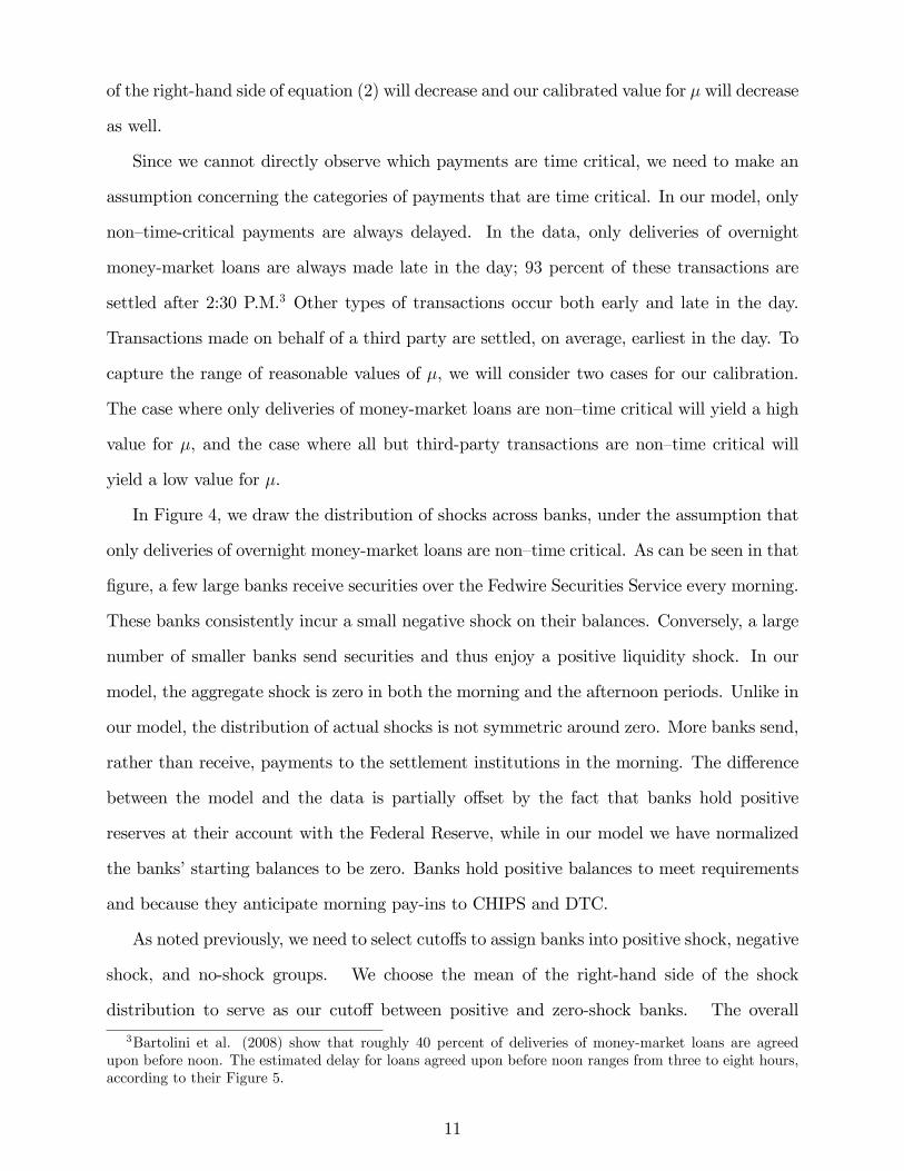
In Figure 4, we draw the distribution of shocks across banks, under the assumption that

only deliveries of overnight money-market loans are non—time critical. As can be seen in that

figure, a few large banks receive securities over the Fedwire Securities Service every morning.

These banks consistently incur a small negative shock on their balances. Conversely, a large

number of smaller banks send securities and thus enjoy a positive liquidity shock. In our

model, the aggregate shock is zero in both the morning and the afternoon periods. Unlike in

our model, the distribution of actual shocks is not symmetric around zero. More banks send,

rather than receive, payments to the settlement institutions in the morning. The difference

between the model and the data is partially offset by the fact that banks hold positive

reserves at their account with the Federal Reserve, while in our model we have normalized

the banks’starting balances to be zero. Banks hold positive balances to meet requirements

and because they anticipate morning pay-ins to CHIPS and DTC.

As noted previously, we need to select cutoffs to assign banks into positive shock, negative

shock, and no-shock groups. We choose the mean of the right-hand side of the shock

distribution to serve as our cutoff between positive and zero-shock banks. The overall

3Bartolini et al. (2008) show that roughly 40 percent of deliveries of money-market loans are agreedupon before noon. The estimated delay for loans agreed upon before noon ranges from three to eight hours,according to their Figure 5.

11

average shock is represented by the middle vertical line in Figure 4 at −0.5 percent. Because

the shock in our model is symmetric, we focus on one side of the distribution and extrapolate.

We choose the right-hand side of the distribution, because small changes in the cutoff will

have only minor effects on our calibration of the shock.4 The mean of the right-hand side

of the distribution is 8.8 percent, which gives a calibrated value for 1 − µ of 9.3 percent.

Thirteen percent of the banks have a shock greater than 0.088. Thus, our calibration of σ

is 0.13. To have a symmetric shock, the cutoff for a negative liquidity shock must be set at

−8.5 percent. This is slightly less than the mean of the left-hand side of the distribution,

which is −7.2 percent.

As expected, the calibrated value for µ decreases as we classify more payments as non—

time critical. If we classify only third-party transactions as time critical, the mean shock,

given by equation (2), is −1.0 percent. The mean value of the right-hand side of the distri-

bution of shocks is 16.5 percent, resulting in 82.5 percent as our calibrated value of µ (since

1 − µ = 17.5 percent). Seventeen percent of the banks have a shock that is greater than

0.165, giving us a calibrated value of 0.17 for σ.

Figure 4: Distribution of shocks. The three vertical lines give the mean shock of the left-hand side of the distribution, the mean shock, and the mean shock of the right-hand side ofthe distribution.

Since µ is greater than 23, welfare under an LSM will be at least as high as under an

RTGS system (see proof of proposition 10 of Martin and McAndrews 2008). Thus, our

4Focusing on the left-hand side of the distribution of shocks leads to little change in the calibrated valuesfor σ and µ.

12

results suggest that welfare would increase if an LSM were added to Fedwire. For an idea of

the size of possible benefits, we compute the ratio of costs under the two different settlement

systems,

ρ =Aggregate cost under RTGSAggregate cost with an LSM

,

for different values of µ and σ in the range of the calibrated value.5 Since we have not yet

attempted to calibrate θ, R, and γ, we let these parameters take a wide range of values.6 As

mentioned in section 2, there are regions of the parameter space for which multiple equilibria

can coexist when a liquidity-saving mechanism is not present. When computing the aggregate

cost under RTGS, we consider the equilibria that have the most payments settle early. This

will imply that our measure is a lower bound for the improvement generated by a liquidity-

saving mechanism. Over this grid, the median value of ρ is 3.13. For more than 90 percent

of the parameter combinations, ρ is greater than 1.45.

The planner always chooses to have all payments sent early for µ greater than 23. For the

same set of parameter values for µ, σ, γR, and θ, the ratio

Aggregate cost under RTGSAggregate cost under a planner’s solution

has a median value of 8.27 and is always at least 1.0625.

To go further and provide an estimate of the benefits of an LSM in dollar terms, we need

to calibrate θ, γ, and R. We do this in the remainder of this section. When calibrating these

parameters, we again consider the case where only money-market deliveries are classified as

non—time-critical payments and the case where deliveries on overnight money-market loans,

returns on overnight money-market loans, and interbank transactions are non—time-critical

payments.

5We choose µ ∈ {0.80, 0.805, ...0.945} and σ ∈ {0.10, 0.11, ..., 0.20}.6We let γ

R ∈ {0.10, 0.13....3.10} and θ ∈ {0.025, 0.075, ...0.975}.

13

3.3 Calibrating θ

Our first step is to calibrate θ. In our model, each bank must make either one time-critical or

one non—time-critical payment. The fraction of banks that must make a time-critical payment

is θ. Since, in the data, banks make both time-critical and non—time-critical payments, we

use an indirect strategy to obtain a value for θ. We exploit the fact that the amount of

reserves borrowed in the model depends only on µ and σ, which we have already calibrated,

and on θ. We choose θ so that the average amount borrowed in Fedwire is consistent with

the amount predicted by our model, given the calibrated values for µ and σ.

The amount of borrowing in the model depends on which equilibrium is played. Martin

and McAndrews (2008) show that four types of equilibria can occur in an RTGS system: (1)

All time-critical payments are delayed, (2) only banks with a positive liquidity shock make

their time-critical payments early, (3) banks with a positive liquidity shock and banks with

no liquidity shock make their time-critical payments early, and (4) all time-critical payments

are made early. Given a calibrated value of σ between 0.13 and 0.17, we should observe that

the fraction of time-critical payments that are delayed is 0 percent, 13− 17 percent, 83− 87

percent, or 100 percent, depending on the type of equilibrium.

Looking at the data, we see that the fraction of payments delayed depends on when we

choose the cutoff between morning and afternoon. If we choose the cutoff time to be noon

and assume that only deliveries of overnight money-market loans are non—time critical, then

82 percent of the time critical payments in our model are delayed. This number would drop

to 72 percent if the cutoff were 2:00 P.M. We get similar values (81 percent for noon and 68

percent for 2:00 P.M.) when only transactions made on behalf of a third-party are classified

as time-critical. In either case, we conclude that Fedwire is in an equilibrium in which only

banks that receive a positive liquidity shock make their time-critical payments early. All

other payments are delayed.

In this equilibrium, theory indicates that the total borrowed from the central bank is

equal to σθ(2µ − 1)(1 − σθ) + σ(1 − σθ)(1 − µ). This expression corresponds to the share

of banks with a time-critical payment and positive liquidity shock, σθ, multiplied by the

14

amount these banks have to borrow if they do not receive a payment in the morning, 2µ−1,

multiplied by the probability that they will not receive a payment in the morning, 1 − σθ,

plus the share of banks with a negative liquidity shock, σ, that do not receive a payment in

the morning, 1− σθ, and must borrow 1− µ.

In the first two quarters of 2007, the average daily amount paid in overdraft fees was

$508, 000 per day. Hence, the number of overdraft hours is 1.219 trillion on the average day.7

We know that the average overdraft was three hours and 59 minutes in the first half of 2007,

implying that approximately $305 billion was borrowed each day from the Federal Reserve

during this period. This amount represents 7.1 percent of the $4.31 trillion sent each day.

Setting σθ(2µ− 1)(1− σθ) + σ(1− σθ)(1− µ) equal to 0.071 gives us combinations of σ, θ,

and µ, which are consistent with our model. These values are plotted in Figure 5. We also

plot the two (µ, σ) pairs calibrated in the previous subsection.

Figure 5 shows that our calibration with fewer payments classified as time-critical (µ =

0.825 and σ = 0.17) results in a smaller value for θ. This accords with our intuition since

we would expect that fewer time-critical payments would lead to a smaller calibrated value

of the share of banks having to make a time-critical payment.

θ =0.0

θ =1.0

θ =0.5

.05

.1

.15

.2

.25

σ

.5 .6 .7 .8 .9 1µ

Figure 5: Values of θ, µ, and σ for which the data are consistent with the model. The two(µ, σ) pairs, as calibrated in the previous subsection, are the two dots in the figure.

7Banks pay 36 basis points, at an annual rate, on their average intraday overdraft. If banks pay $508, 000per day, then their aggregate intraday overdraft is $ 508,000

36 basis points/year*1year/360 days*1 day/24 hours = 1.219 trilliondollar-hours.

15

In summary, Figure 5 shows that values of θ in the range (13, 23) are consistent with the

values of µ and σ that were calibrated in section 3.2.

3.4 Calibrating γ and R

Using the calibrated values of µ, θ, and σ, we can calibrate γR, the ratio of the cost of delay

to the daylight overdraft fee. Then, to complete our calibration, we calibrate R based on

the overdraft fee paid by banks. Our strategy is to choose a value of γRsuch that the timing

of settlement given by the model is consistent with the timing of settlement in the data. In

our model, all non—time-critical payments are delayed. Banks will choose to send or delay

time-critical payments depending on the magnitude of γRand on their liquidity shock.

If only banks with a positive liquidity shock make their time-critical payments early, as we

argued in the previous subsection, then we must have (1−σθ)µ > γR≥ (1−σθ)(2µ−1). This

gives us a range of 0.830 > γR≥ 0.738 using our calibration with many payments classified as

time critical (µ = 0.90, σ = 0.13, and θ = 0.60) and a range of 0.769 > γR≥ 0.606 using our

calibration with few payments classified as time critical (µ = 0.825, σ = 0.17, and θ = 0.40).

Next we calibrate R: Fedwire participants pay 36 basis points to the Federal Reserve on

their average daylight overdrafts. Since the average length of an overdraft is three hours and

59 minutes, our calibrated value of R is 6.0 (= 363.9924) basis points.

Given our calibration for R, µ, θ, and σ, there is a range of values of γ consistent with

the RTGS equilibrium we consider. For such values of γ, two kinds of equilibria can occur

with an LSM. For example, with R = 6, µ = 0.90, σ = 0.13, and θ = 0.60, if we let γR= 0.79

then all payments are made early with an LSM. For these parameters, the cost of using the

payment system is $78, 000 per day with an LSM but $2.88 million per day with RTGS. If,

instead, γR= 0.83, then in an LSM equilibrium, banks with positive shocks send time-critical

payments early, banks with negative shocks delay their non—time-critical payments, and all

other payments are queued. The cost of using the payment system is $1.24 million with

an LSM but $3.11 million with RTGS. Similar results hold under the assumption of fewer

time-critical payments. With R = 6, γR= 0.68, µ = 0.82, σ = 0.17, and θ = 0.40, the cost of

16

using the payment system is $1.76 million with RTGS but only $1.10 million with an LSM.

Our results indicate that the calibrated benefits of using an LSM can vary from approxi-

mately $500, 000 a day to more than $2 million a day, depending on the calibration. We can

compare this benefit to the estimated cost the ECB planned to charge the users of TARGET

2 for its liquidity-pooling features. The annual cost is estimated at Euro 900, 000 (ECB

2005). Hence, even for the calibrations that yield relatively small benefits from using an

LSM, these benefits appear large compared to the cost.

The calibration exercise reveals another interesting fact: The cost of borrowing from

the central banks can be small compared to the cost imposed by delay. For example, with

parameters set to R = 6, γR= 0.79, µ = 0.90, σ = 0.13, and θ = 0.60, as above, the borrowing

cost makes up only approximately 18 percent($508, 000 / $2.88 million) of the total costs

of participating in the payment system. Hence, considering only the cost of borrowing can

substantially underestimate the actual cost of using the payment system.

3.5 Discussion

What determines the size of the improvements associated with implementing a liquidity-

saving mechanism? The total cost incurred by banks in participating in the large-value

system consists of two components. First, banks pay overdraft fees to the central bank. We

can easily take this component of the total welfare cost from existing data. As mentioned

above, the Federal Reserve collects roughly $500,000 per day in overdraft fees. The second

component, delay costs, is impossible to observe directly. Here, we rely on our model to get

a sense of how large aggregate delay costs are, relative to overdraft costs. Banks both delay

and send some of their payments early. In 2006, 50 percent of the value of Fedwire activity

was settled after 4:15 P.M., two hours and fifteen minutes before Fedwire closes (Armantier

et al. 2008). From the observed distribution of payment settlement times, we make the

following conclusions. First, there are many payments for which delay costs are incurred.

Second, we are able to restrict the ratio of the cost of delaying a payment to the cost of

borrowing from the central bank. Given our model, we calibrated that the cost of delaying

17

a payment is somewhere between 60 percent to 85 percent of the cost of borrowing from the

central bank. Furthermore, given the distribution of payment settlement times, we see that

banks do, indeed, delay a large fraction of their payments. Putting the last two sentences

together, we conclude that the aggregate delay costs incurred by banks is on the same order

of magnitude or larger than the aggregate welfare costs associated with overdraft fees.

When a liquidity-saving mechanism is introduced, as long as the liquidity shock is not

too large (1 − µ < 13) the only banks that delay their payments outright are those with a

negative liquidity shock and non-time-critical payments. All other banks either queue or

send their payments early. This has two effects. First, as fewer banks with a positive or zero

liquidity shock delay their payments, liquidity is transferred from banks with positive and

zero liquidity shock to banks with negative liquidity shock, causing a reduction in aggregate

overdraft fees. Second, by examining Table 2 and Figure 3, we see that, for most parameter

combinations, all time-critical payments are released in the morning, driving aggregate delay

costs to zero. There are some parameter combinations—those associated with equilibrium

#3 in Figure 3—where zero-and-negative-liquidity-shock banks with a time-critical payment

queue, rather than send their payment outright. As long as the fraction of banks with a

non-time-critical payment is not too large, a large fraction of these queued payments will

be released in the morning.8 So, introducing a liquidity-saving mechanism either eliminates

aggregate delay costs or, if the fraction of banks with a time-critical payment is not too

small, reduces the size of aggregate delay costs by a considerable amount. To sum up the

argument of this paragraph and the one before, the benefits of an LSM are on the same order

of magnitude as the aggregate amount paid in delay costs, which are as large or larger than

the aggregate amount paid in overdraft fees to the central bank, $500,000 per day. The key

ingredients to these conclusions were that γRis not too close to zero, the fraction of banks

with a time-critical payment is not too small (θ is not too close to zero), and the liquidity

shock is not too large (µ > 23).

There are two possible ways in which our calibrated value of the aggregate welfare im-

8In particular, the fraction of these queued payments that are released in the morning is equal to thefraction of banks with a time-critical payment.

18

provement may differ from the actual benefit accrued by the Federal Reserve. On the one

hand, our calibrated value may overstate the benefit of a liquidity-saving mechanism. In

our model, all payment orders occur at the beginning of the day. In reality, this may not

be the case. So, what we capture in our calibration as a delayed payment may actually be

a payment order occurring later in the day. Since we are overstating the calibration of the

value of payments delayed in an RTGS, we are also overstating the benefit of an LSM. On

the other hand, our calibrated value may understate the benefit to the Federal Reserve of

implementing an LSM. Above, we calibrate only the benefit of an LSM to payment system

participants. However, the Federal Reserve has an additional interest in moving payments

away from the very end of the day because of concerns over operational risks. These benefits

of a more robust payment system would also be broadly shared by participants.

3.6 Sensitivity analysis

We have already seen that, depending on which payments are classified as time critical, our

calibrated value of 1 − µ can vary by a factor of two and our calibrated benefits vary from

over $2 million per day to roughly $500, 000 per day. In addition, we have allowed θ to

vary over a wide interval, showing that changes in the fraction of banks with a time-critical

payment do not materially affect the calibrated gains from a liquidity-saving mechanism. In

this section, we discuss three additional robustness checks. These three scenarios will affect

our calibrated values of µ and σ. Changing µ and σ will cause our calibrated values of θ and

γRto change as well, as the calibration of these two parameters involves calculations in terms

of µ and σ. The robustness checks confirm that there are large benefits to implementing an

LSM.

Below, we consider how robust the calibrated results are to:

• changing the cutoff between banks that receive a positive liquidity shock and those

that receive a zero liquidity shock. In the original calibration, we set the cutoff to be

the mean of the right-hand side of the distribution of shocks.

• changing the cutoff between the morning and afternoon periods. In the original cali-

19

bration, we set the cutoff to be noon.

• changing the sample period. Armantier et al. (2008) find that, on certain days, pay-

ments are settled on Fedwire significantly earlier. In particular, on days before or after

a holiday, on the last day of the quarter, on the first day of the month, or on the 15th

or 25th of the month9 the median payment is settled 10-20 minutes earlier.

The results of the robustness exercises are summarized in Table 3, below. Up to this

point, we have performed our calibration exercise under two different assumptions on which

categories of payments are time critical. To save space we will report only the sensitivity

analysis for the case where many payments are classified as non-time critical. Compared

to this case, when more payments are classified as time critical, we find that calibrated

values of µ are consistently larger, calibrated values of σ tend to be smaller, and the welfare

improvement tends to be larger.

In the first three rows, we describe the effect of changing the cutoff between positive-

liquidity-shock banks and zero-liquidity-shock banks. We can visualize this changing cutoff

as moving the right-most vertical line in Figure 4 to the left or right. Shifting the cutoff to

the right mechanically increases µ and σ. Remember that we calibrated θ using the following

equation describing the amount paid in overdraft fees to the central bank: σθ(2µ−1)(1−σθ)+

σ(1− σθ)(1− µ) = 0.071. A higher σ implies a lower calibrated value for θ. The calibrated

fraction of time-critical payments can vary considerably, increasing above 0.95 when µ is

small. Increasing the cutoff between banks with positive and banks with zero liquidity

shock increases the calibrated welfare improvement of a liquidity-saving mechanism, mainly

because the calibrated fraction of payments that are classified as time critical (and thus

subject to a delay cost) has increased. Decreasing the cutoff also increases the calibrated

welfare improvement, but for a different reason. When we set the cutoff to be 12times

the mean of the right-hand-side of the shock distribution, the other calibrated parameters

imply that, in equilibrium with a liquidity-saving mechanism, all payments are settled in the

9On these days, Fannie Mae and Freddie Mac make interest and redemption payments on mortgage-backedsecurities.

20

morning period. In this part of the parameter space, shifting all payments to the morning

period leads to a large welfare improvement.

In the fourth, fifth, and sixth rows of Table 3, we describe the effect of changing the

cutoff time between the morning and afternoon periods. Shifting the cutoff to later in the

day leads to a lower σ and a higher θ. Having a larger calibrated fraction of time-critical

payments implies that the welfare gains will be larger.

In the final two rows, we examine whether our results are sensitive to the sample of days

that we used. The parameter values do not change when we restrict the sample to days that,

according to Armantier et al. (2008), have earlier-than-average settlement of payments.

+/0 Time Sample µ σ θ γR

LSM Equilibria Improvement1× 12 All 0.82 0.17 0.39 [0.60, 0.77] 1if γ

R< 0.64; 3otherwise ∼$700, 000

0.5× 12 All 0.94 0.24 0.30 [0.82, 0.87] 1 ∼ $1, 600, 0001.5× 12 All 0.74 0.11 0.96 [0.43, 0.66] 1if γ

R< 0.48; 3otherwise ∼ $3, 100, 000

1× 12 All 0.82 0.17 0.39 [0.60, 0.77] 1if γR< 0.64; 3otherwise ∼ $700, 000

1× 10 All 0.70 0.15 0.53 [0.37, 0.64] 1if γR< 0.40; 3otherwise ∼ $900, 000

1× 2 All 0.82 0.10 0.94 [0.58, 0.74] 1if γR< 0.64; 3otherwise ∼ $3, 700, 000

1× 12 All 0.82 0.17 0.39 [0.60, 0.77] 1if γR< 0.64; 3otherwise ∼ $700, 000

1× 12 Subset 0.81 0.18 0.38 [0.58, 0.76] 1if γR< 0.62; 3otherwise ∼ $700, 000

Table 3: Results from the robustness exercises. The first three rows display the effect ofchanging the cutoff between banks that receive a positive versus zero liquidity shock. Thesecond three lines consider the effect of changing the cutoff between morning and afternoonperiods. The last two rows consider the effect of changing the sample period. In the "LSMEquilibria" column, the number 1 indicates that all payments are settled early and the number3 indicates that s+ banks pay early, r- banks delay, and all other banks queue their payments.

The sensitivity analysis we have performed in this section implies that our original

estimate of the potential gains of a liquidity-saving mechanism may be on the conservative

side. There is still reason to be cautious, however, as the calibrated values for θ, γRand the

welfare gains do vary considerably.

4 Conclusion

Our calibration is the first attempt to use data to evaluate the potential impact of an LSM.

We use Fedwire data to calibrate the parameters of our model. We then use these calibrated

21

parameters to determine what an equilibrium would look like with an LSM. By comparing

the two equilibria, we can derive the potential benefit from adopting an LSM. Our results

suggest that the benefits of an LSM can be significant. In particular, we find that even with

the calibration that assigns the smallest benefit from using an LSM, it would take only a

few days to make up the fixed cost of setting up such a system. Our calibration also shows

that the observed cost of borrowing can be small compared to the overall cost of using the

payment system.

5 References

Armantier, O., Arnold, J., McAndrews, J., 2008. Changes in the Timing Distribution ofFedwire Funds Transfers. Economic Policy Review, Federal Reserve Bank of New York,83-112.

Angelini, P., 1998. An analysis of competitive externalities in gross settlement systems.Journal of Banking and Finance 22, 1-18.

Angelini, P., 2000. Are banks risk averse? Intraday timing of operations in the interbankmarket. Journal of Money, Credit and Banking 32, 54-73.

Atalay, E., Martin, A. McAndrews J., 2010. The Welfare Effects of a Liquidity-SavingMechanism. Staff Report 331, Federal Reserve Bank of New York.

Bartolini, L., Hilton, S., McAndrews, J. J., 2008. Settlement Delays in the Money Market.Staff Report 319, Federal Reserve Bank of New York.

Bech, M. L., Garratt, R., 2003. The Intraday Liquidity Management Game. Journal ofEconomic Theory 109, 198-219.

BIS, 2005. New developments in large-value payment systems. CPSS Publications No. 67.

ECB, 2005. Progress report on TARGET 2. http://www.ecb.int/pub/pdf/other/target2progressreport200502en.pdf.

Johnson, K., McAndrews, J. J., Soramaki, K., 2004. Economizing on Liquidity with DeferredSettlement Mechanisms. Economic Policy Review, Federal Reserve Bank of New York, 51-72.

Lester, B., 2009. Settlement Systems. The B.E. Journal of Macroeconomics 9.

Martin, A., 2004. Optimal pricing of intraday liquidity. Journal of Monetary Economics 51,401 —424.

22

Martin, A., McAndrews, J., 2008. Liquidity-saving Mechanisms. Journal of Monetary Eco-nomics 55, 554-567.

Martin, A., McAndrews, J., 2010. Should there be intraday money markets? ContemporaryEconomic Policy 28, 110-122.

Mills, D. C. Jr., Nesmith, T. D., 2008. Risk and Concentration in Payment and SecuritiesSettlement Systems. Journal of Monetary Economics.

Roberds, W., 1999. The Incentive Effect of Settlement Systems: A Comparison of GrossSettlement, Net Settlement, and Gross Settlement with Queuing. IMES Discussion PaperSeries, 99-E-25, Bank of Japan.

A Additional Results from Martin and McAndrews(2008) (not necessarily for publication)

In section 2, we presented a review of the results of Martin and McAndrews (2008). For themost part, we emphasized the qualitative results of the model. For the sake of completeness,we include the main propositions of Martin and McAndrews (2008). These propositionsdescribe the regions of the parameter space for which different equilibria occur.The equilibria without an LSM are characterized in proposition 2 of Martin and McAn-

drews (2008). Without an LSM, multiple equilibria can coexist for certain regions of theparameter space.

Proposition 1 Four equilibria can exist. For all equilibria, non—time-critical payments aredelayed. In addition,

1. If γ ≥ [µ− θ(2µ− 1)]R, it is an equilibrium for all time-critical payments to be sentearly.

2. If {µ− θ (1− σ) (2µ− 1)}R > γ ≥ [1− θ (1− σ)]µR, then it is an equilibrium forbanks of type s− to delay time-critical payments while other banks pay time-criticalpayments early.

3. If (1− σθ)µR > γ ≥ (1− σθ)(2µ− 1)R, it is an equilibrium for only banks of type s+to send time-critical payments early.

4. If (2µ− 1)R > γ, then it is an equilibrium for all banks to delay.

The equilibria with an LSM are characterized in proposition 6 of Martin and McAndrews(2008).

Proposition 2 With a liquidity-saving mechanism, the following equilibria exist:

1. If γ < (2µ− 1)R, then all banks queue their payment.

2. If γ ≥ (2µ− 1)R and µ ≥ 2/3, then

23

(a) If γ ≥ µR, then all time-critical payments are sent early. Banks with a negativeliquidity shock delay non—time-critical payments, and non—time-critical paymentsfrom other types of banks are queued.

(b) If µR > γ ≥ (2µ − 1)R, then only banks with a positive liquidity shock sendtime-critical payments early. Banks with a negative liquidity shock delay non—time-critical payments, and all others queue their payment.

3. If γ ≥ (2µ− 1)R and µ < 2/3, then

(a) If γ ≥ µR, the equilibrium is the same as under 2a.

(b) If µR > γ ≥ (1− µ)R , the equilibrium is the same as under 2b.

(c) If (1−µ)R > γ ≥ (2µ−1)R, then banks that receive a negative liquidity shock delaytheir payment. Banks that receive a positive liquidity shock send their time-criticalpayment early. All other payments are queued.

24