Feature generation and selection - ru

Automatic feature generation andselection in predictive analytics

solutions

Suzanne van den Bosch

Suzanne van den Bosch: Automatic feature generation and selection in predictiveanalytics solutionsMaster thesis Computing ScienceFaculty of Science, Radboud UniversityStudent number: s4021444

Supervisors:Arjen de Vries, Radboud UniversityEdwin de Jong, QuintiqStieneke de Lange, Quintiq

Nijmegen, June 2017

2 Automatic feature generation and selection in predictive analytics solutions

Abstract

In this thesis we proposed a feature generation and selection method called Fea-ture Extraction and Selection for Predictive Analytics (FESPA). This methodaims to improve the current Predictive Analytics solution of Quintiq, which hadonly options for manual feature selection and no options for feature generation.We have discovered that the proposed method does not decrease performance.In most cases, however, it does also not improve the performance. For the datasets where the performance increased, the improvement is significant.

Automatic feature generation and selection in predictive analytics solutions iii

Acknowledgements

I would like to thank a number of people who have supported me during theprocess of this master thesis.

First, I would like to thank Arjen de Vries, for giving me advice about thedirection of my research, for ensuring me I did not have to be stressed aboutlittle things like the final presentation when it is still two months away, and forhelping me whenever I got stuck in figuring out the ExploreKit algorithm, theimplementation or the writing of this thesis. I would also like to thank ElenaMarchiori for taking the time and effort to be the second reviewer for this thesis.

I would like to thank my colleagues and supervisors at Quintiq. Edwin deJong for giving me the opportunity to do this research at Quintiq, for helping medefine the scope of this thesis, and giving me the freedom to define a researchscope that appealed to me most. Stieneke de Lange for patiently explainingthe perspective of the user to me and for the useful feedback while writing thisthesis. That made this thesis a lot more readable. Harm Buisman for all hishelp with understanding the Predictive Analytics solution and feedback on myimplementation of FESPA in the Quintiq software.

Last, but certainly not least, I would like to thank my boyfriend Frank Blomand my parents, Rob and Marieke, for all their loving support and unwaveringtrust in my capabilities. Without them none of this would have been possible.

Automatic feature generation and selection in predictive analytics solutions v

Contents

Contents vii

1 Introduction 11.1 Feature generation . . . . . . . . . . . . . . . . . . . . . . . . . . 21.2 Feature selection . . . . . . . . . . . . . . . . . . . . . . . . . . . 31.3 Quintiq . . . . . . . . . . . . . . . . . . . . . . . . . . . . . . . . 31.4 Thesis structure . . . . . . . . . . . . . . . . . . . . . . . . . . . . 4

2 Related Work 52.1 Decision tree . . . . . . . . . . . . . . . . . . . . . . . . . . . . . 52.2 Information Gain . . . . . . . . . . . . . . . . . . . . . . . . . . . 62.3 ExploreKit . . . . . . . . . . . . . . . . . . . . . . . . . . . . . . 62.4 Other methods . . . . . . . . . . . . . . . . . . . . . . . . . . . . 7

3 Methods 93.1 Feature generation . . . . . . . . . . . . . . . . . . . . . . . . . . 9

3.1.1 Unary Operators . . . . . . . . . . . . . . . . . . . . . . . 93.1.2 Binary Operators . . . . . . . . . . . . . . . . . . . . . . . 103.1.3 Group-by-then operators . . . . . . . . . . . . . . . . . . . 103.1.4 Redundant operators . . . . . . . . . . . . . . . . . . . . . 113.1.5 Linear transformations . . . . . . . . . . . . . . . . . . . . 11

3.2 Feature selection . . . . . . . . . . . . . . . . . . . . . . . . . . . 123.2.1 Meta-features . . . . . . . . . . . . . . . . . . . . . . . . . 133.2.2 Background learner . . . . . . . . . . . . . . . . . . . . . . 13

4 Results 154.1 Performance . . . . . . . . . . . . . . . . . . . . . . . . . . . . . . 154.2 Influence background collections . . . . . . . . . . . . . . . . . . 184.3 Operators . . . . . . . . . . . . . . . . . . . . . . . . . . . . . . . 194.4 Growth of number of features . . . . . . . . . . . . . . . . . . . . 204.5 Run-time approximation . . . . . . . . . . . . . . . . . . . . . . . 21

5 Discussion 235.1 Performance . . . . . . . . . . . . . . . . . . . . . . . . . . . . . . 235.2 Influence background collections . . . . . . . . . . . . . . . . . . 245.3 Operators . . . . . . . . . . . . . . . . . . . . . . . . . . . . . . . 245.4 Time versus accuracy . . . . . . . . . . . . . . . . . . . . . . . . 245.5 Future work . . . . . . . . . . . . . . . . . . . . . . . . . . . . . . 25

Automatic feature generation and selection in predictive analytics solutions vii

CONTENTS

Bibliography 27

Appendix 29

A Overview data sets 29

B Algorithms pseudo-code 30

viii Automatic feature generation and selection in predictive analytics solutions

Chapter 1

Introduction

Data processing is the collection and manipulation of data. In this thesis, wefocus on data processing involving machine learning.

The focus of machine learning research has mainly been on the learningalgorithms. This may be due to the limited amount of available data. Over theyears, the available technology became more advanced and that has created thepossibility to store significantly more data. With the increase of data, it hasbecome clear that the representation of the data, which is the input of a learningalgorithm, can have a significant impact on the performance of that learningalgorithm. Currently, there is more available data, but that data contains morenoisy and relatively less useful data. Therefore, adequate data pre-processing isbecoming more and more important.

Data pre-processing is a collective name for all methods that aim to ensurethe quality of the data. We focus on two methods within data pre-processingcalled feature generation and feature selection, explained in more detail in Sec-tion 1.1 and 1.2 respectively.

Besides feature generation and feature selection, there is a process whichaims to detect and correct inconsistent and missing values in the data. Thisprocess is called data cleaning. Data cleaning is also an important part of thedata pre-processing phase, but is out of the scope of this thesis.

In this thesis, we address the problem of efficient and effective feature gener-ation and feature selection for a specific machine learning problem. We proposea method that will improve the current Predictive Analytics solution of Quintiq,described further in Section 1.3. The proposed method is based on an existingimplementation of a feature generation and selection method called ExploreKit,further discussed in Section 2.3.

Our research objective of improving the current Predictive Analytics solutionfor Quintiq has two aspects that need to be taken into account; first the scientificresults should be improved, however since the tool is used by companies inpredicting planning aspects on the short until long term horizon it also meansit should produce results in a timely manner. This means that, as part of ourresearch, we are not going for the optimum scientific solution, but we try to finda balance between improved results and fast results. Since this balance can bedifferent for each business case, the approach we took aims to make the resultingPredictive Analytics solution flexible and configurable by the user. One exampleis that feature generation and selection methods have been split and can be run

Automatic feature generation and selection in predictive analytics solutions 1

CHAPTER 1. INTRODUCTION

separately, as well as the fact that their parameters can be set.

1.1 Feature generation

Feature generation is also known as feature construction, feature extraction orfeature engineering. There are different interpretations of the terms featuregeneration, construction, extraction and engineering. Some nearly equivalent,yet differing definitions for these terms are; construction of features from rawdata [11, 6], creating a mapping to convert original features to new features [12],creating new features from one or multiple features [10].

In the context of this thesis, feature generation and all its synonyms will beinterpreted as the process of creating new features from one or multiple features,unless otherwise specified.

Two goals of feature generation can be dimensionality reduction and ac-curacy improvement [13, 4]. When the goal of a feature generation method isdimensionality reduction, then the result will be a feature space which containsless features than the original feature space. However, when the goal is accuracyimprovement, the resulting feature space will most likely contain more featuresthan the original feature space.

We are primarily interested in feature generation methods where the goalis to improve the accuracy of the predictor. Dimensionality reduction does nothave a high priority, since the results of feature generation are input to a featureselection phase aims to reduce the dimensionality of the feature space. Eventhough the feature generation phase does not have to reduce the dimensionality,it certainly has to take care to not generate an extreme amount of new features.

To illustrate the importance of feature generation, consider the followingexample in Table 1.1. Here we can see the original feature Date and dependentfeature Visitors, which shows a date and the corresponding number of visitorsfor a theme park. When looking at just these features, there does not seem tobe an obvious pattern between the predicting and the dependent feature. Withfeature generation, we can extract what kind of day the date is, shown in theIsWeekendDay column. This tells us whether the date is a weekend day or not.Now we can see a clear pattern where the number of visitors is significantlyhigher on weekend days than on week days.

Date Visitors IsWeekendDay

‘20-05-17’ 19234 yes‘11-04-17’ 5735 no‘29-01-17’ 17914 yes‘04-05-17’ 5496 no‘29-03-17’ 5913 no

Table 1.1: Example features Day and Visitors and extracted feature IsWeek-endDay{Day}

Another situation where feature generation can improve performance is whenthere is feature interaction. Then two (or more) features are not relevant orcorrelated to the dependent feature on their own, but together they have a(high) influence on the dependent feature. For example, take as features the



price and quality of a product. Separately, they will not give much indication ofwhether a product is purchased often. Combined they have a high correlationto the purchase of the product. If the price is low and the quality high, then theproduct will be purchased often. However, a low price or a high quality withoutknowing the other value cannot guarantee that the product will be purchasedoften. If both price and quality are low, then the product will not be purchasedby many customers. The same can be said when both price and quality arehigh.

1.2 Feature selection

Feature selection tries to find the optimal subset of a given feature set. Theproblem of feature selection is essentially equivalent to the problem of findingthe optimal subset of a given set, which has been shown to be NP-hard. There isone simple method to find the optimal subset, namely calculate the evaluationscore for each possible subset. The advantage of this method is that it willalways find the optimal subset. A disadvantage is that the complexity is O(2n),where n is the number of features. This means that for 10 features, already 1024sets have to be evaluated. This disadvantage is even more influential, becausefeature selection will become more useful the more features are involved.

Since evaluating every subset separately is practically infeasible, there isneed for a different, smarter way to decide the usefulness of each subset.

If the original feature set contains a thousand features, it is highly likelythat not all features positively influence the dependent variable. For example,in text mining it is common practice to remove the stop words; the, in, a, of,as, and, with, and many more. Although stop word removal can be seen as apart of the data cleaning step, it can also be seen as a separate feature selectionstep. Consider every word to be a feature, then the stop words are features thatdo not contribute to the prediction of the dependent value.

Feature irrelevance is the problem that some features are simply not correl-ated to the dependent feature. These features can even have a negative effecton the performance of a model.

1.3 Quintiq

Quintiq is one of the top companies in supply chain planning and optimization.It was started in 1997 as a scheduling company by five programmers. It hassince grown to a vast company with offices all around the world and over 12 000users every day. They have been developing a predictive analytics solution asa stand-alone product or to improve other products. The predictive analyticssolution as it is at the start of this research had several functionalities. It givesusers the option to load in their own data-set, manually select and deselectfeatures, train a decision tree and use that tree to predict new values. Thesolution helps users select features by giving them the option to calculate theerror per feature. With the feature generation and selection method proposedin this thesis, we aim to improve the performance compared to no selection andmanual selection.

Since the classifier method implemented in the Quintiq predictive analytics



solution is a decision tree, the proposed method in this thesis only has decisiontrees in its scope. The decision trees implemented in this thesis are based onthe definition by Breiman [2].

1.4 Thesis structure

In section 2, we discuss the literature that is relevant to this thesis. In section3, we discuss the method that is implemented in this thesis. In section 4, theempirical results are discussed. In section 5, we discuss the implications of theresults and conclusions.


Chapter 2

Related Work

In this section, we discuss research done that is relevant for the research donein this thesis. Feature generation and selection methods have been shown toimprove the performance of machine learning tasks [9, 5, 14].

2.1 Decision tree

The learning algorithm used in this thesis is a decision tree based on the bookby Breiman [2]. The decision tree algorithm builds an acyclic connected graph.Each node represents one of the input features.

Take Figure 2.1 as example. This Figure represents a decision tree build ondata of passengers of the Titanic. The input features are the sex and age of thepassengers. Based on a part of the data, the decision tree makes a decision ineach node and determines the class that decision most likely belongs to. Forexample, this decision tree would predict that a male passenger of age thirtywill have died on the Titanic.

Figure 2.1: Example: Titanic data set


CHAPTER 2. RELATED WORK

2.2 Information Gain

Information Gain is used as a baseline for the proposed method in this thesis.Information Gain is a method that can be applied to a learning algorithm tofind how much information every feature contains.

For a decision tree, it will look at the nodes and for each node calculate howmuch information is gained by the split. For example, consider the decisiontree in Figure 2.2(a). Here the distribution of the classes stays consistent whensplitting from the root to the two leaf nodes. This means that doing this splithas gained the learner no new information. Feature Z will therefore have a lowInformation Gain score.

Now consider the decision tree in Figure 2.2(b). Here the distribution ofthe classes completely changed, with class I being contained in the first leaf andclass II being contained in the second leaf. Here the split has gained the learnerall the information it needed. Feature Y will therefore have a high InformationGain score.

(a) (b)

Figure 2.2: Examples of (a) no gain and (b) gain, while using Information Gain

The Information Gain method used in this thesis is the variable importancedefined by Breiman [2].

2.3 ExploreKit

ExploreKit [7] is the inspiration for the implemented method for feature ex-traction and feature selection which is analyzed in this thesis. The methodproposed in this thesis is implemented for regression tasks whereas ExploreKitis implemented for classification tasks. Since we compare method from thisthesis to ExploreKit, we use a subset of the data sets used for ExploreKit. TheExploreKit method provides a combined method for feature extraction and fea-ture selection. The key contribution of this work is to introduce a classifier topredict the usefulness of features extracted.

The ExploreKit algorithm goes as follows. For a fixed number of iterations,they generate candidate features based on the current feature set. F0 is theoriginal feature set. Then they rank the candidate features by a backgroundclassifier. The background classifier is explained in more detail in Section 3.2.Starting with the highest ranking candidate, they evaluate the set containingthe current features and the current candidate feature on the classifier, whichis either a decision tree, support vector machine or random forest. Based onthe outcome of this evaluation, they either (1) add the candidate feature to thecurrent feature set, end the iteration and go to the next iteration, (2) markthis candidate feature as best so far and continue to the next candidate feature


CHAPTER 2. RELATED WORK

in the ranking or (3) discard this candidate feature and continue to the nextcandidate feature.

2.4 Other methods

Several different implementations of feature extraction and selection methodsare FICUS [10], Brainwash [1] and Cognito [8].

FICUS has many similarities to the ExploreKit method, see Section 2.3. Oneof the differences is that FICUS allows for user-specified feature transformationsand constraints. FICUS considers two different categories for transformations,namely domain-independent and domain-dependent.

Brainwash is a method designed to help computer programmers. It considerspieces of code to be features. Based on features that other programmers wroteand used and the features that the current programmer wrote, it recommendsnew features. After the recommendation, the programmer can use the newfeature and give feedback to the system about the usefulness of the new feature.

Cognito implements a greedy incremental search approach. It builds a so-called transformation tree. This transformation tree can be seen as a non-cyclicgraph where the nodes represent data sets and the edges represent transforma-tions of those data sets. The root is the original data set. The tree can then besearched using breadth-first or depth-first search to find the best data set.

The method proposed by Shadvar [15], uses the Mutual Information measureto generate new features from the original features. This method reduces thedimensionality of the feature space.

There are several other methods that may be just as good as or better thanExploreKit. Evolutionary algorithms are one of these methods[3]. The ideabehind evolutionary algorithms is that it starts with some basic blocks andcreates new blocks from combinations of existing blocks. However, evolutionaryalgorithms are so essentially different that discussing them is outside the scopeof this thesis.


Chapter 3

Methods

In this section, the proposed method will be explained in detail. In this thesis,we develop FESPA, Feature Extraction and Selection for Predictive Analytics,inspired by ExploreKit [7], but aiming to be more user-friendly by separatingfeature generation and feature selection into two phases. FESPA consists oftwo separate methods, one for feature generation and one for feature selection.Pseudo-code for all methods is given in Appendix B.

3.1 Feature generation

In order to create new features from old features, we need to define transforma-tions. These transformations define the mapping that will be used to transformone or multiple features into a new feature. The transformations are calledoperators. We use operators from three different categories; unary, binary andgroup-by-then. The three categories are discussed in detail below.

Pseudo-code for the feature generation process is shown in Algorithm 1.Users can choose which operators they want to apply in the feature generationprocess. In the actual implementation the flags doApplyUnary, doApplyBinaryand doApplyGroupByThen are changed to a flag per specific operator instead ofa flag per category. This gives the user full control over which operators areused.

3.1.1 Unary Operators

Unary operators can be any transformation that transforms a single featureinto a new feature. We have defined five different unary operators, motivatedby their use in ExploreKit and described below.

Equal range discretizer The ‘Equal range discretizer’ operator can onlybe applied to numeric features. As the name implies, this operator discretizesthe input feature. The number of groups to which the input feature should bediscretized is a user-configurable constant. From the range of the input featureand the number of groups, it calculates the range per group.

For example, if a numeric feature has a minimum value of 0 and a maximumvalue of 20, then the range of that feature is 20. Take the number of groups to


CHAPTER 3. METHODS

be 10, then the range per group will be 20/10 = 2. The first group will then beall values in the range [0,2], the second group (2,4], etcetera.

Standard score The ‘Standard score’ operator can only be applied to numericfeatures. The resulting feature value is calculated using Equation 3.1.

StandardScore(x) =x− xσx

(3.1)

where x is the average over x and σx is the standard deviation of x.

Day of the week The ‘day of the week’ operator extracts the day of the weekfrom a Date feature. The new value will be a number between zero and six,where zero is Sunday and six is Saturday. This way the learner can better findweekly patterns.

Is weekend The ‘is weekend’ operator converts a Date feature to a logicalfeature. This new feature contains information about whether or not the dateis in the weekend.

Hour of the day The ‘hour of the day’ operator extracts the hour of the dayfrom a time feature.

3.1.2 Binary Operators

The binary operators are defined as follows:

Definition 3.1. Let x and y be numeric features. Let f be a function thatperforms a mathematical operation. A binary operator is defined as f(x,y).

The currently available mathematical operations for these operators are thestandard mathematical operators; addition, division, multiplication.

3.1.3 Group-by-then operators

The group-by-then operators group the data set based on one or multiple fea-tures, called the sources, and perform an action on a separate feature, calledthe target. The action can be one of five mathematical operations; average,maximum, minimum, standard deviation or count. These group-by-then oper-ators can be explained by SQL statements. They are a combination of the GROUPBY statement and an aggregate function. This function can be either MIN, MAX,MEAN, or STDEV. For example, consider the data-set shown in Table 3.1. If ‘Age’is the target feature and ‘Gender’ is the source feature, then the data will begrouped on ‘Gender’. This will result in two groups; ‘Male’ and ‘Female’. As-sume we use the minimum operation, then the resulting new feature will be asshown in the third column. ‘Gender’ can not be the target feature, since it isnot numeric.

There is also a COUNT group-by-then operator, which differs slightly fromother group-by-then operators in that it does not use a target feature. TheCOUNT operator groups the data set based on the source features and then countsthe number of instances per group.


CHAPTER 3. METHODS

Gender Age GBTM

Male 24 24Female 22 22Male 26 24Male 26 24

Female 24 22

Table 3.1: Example features Gender and Age and extracted feature Group-ByThenMinimum{Gender, Age} (GBTM)

3.1.4 Redundant operators

Scaling is a unary operator which was considered, where the resulting featurevalue is calculated using Equation 3.2.

Scaled(x) = cx (3.2)

where c is a constant value and x is the original feature value. The scalingoperator is not implemented, because scaling of a feature has no impact on theoutput of the decision tree. In the decision tree every node contains a decisionabout a feature. Consider the node that decides over feature xi. Let xi > θbe the optimal decision given the current strategy. Then transform xi with ascaling operator; x′i = cxi. If c = 0, then all feature values will become 0 andthat is clearly not desirable. Either, x′i > cθ is the optimal decision if c > 0,because then cxi > cθ ⇔ xi > θ. Or, x′i < cθ is the optimal decision if c < 0,because then cxi < cθ ⇔ xi > θ. Either way, we receive an equivalent optimaldecision.

We have also considered adding subtraction as an additional binary oper-ator. However, the subtraction operator can be defined as the binary addi-tion operator combined with a scaling operator applied to one of the features;sub(x, y) = add(x, Scaled(y)). We have proven that scaling does not influencethe structure of the decision tree and therefore the subtraction operator will beequivalent to the addition operator.

3.1.5 Linear transformations

We take a special look at the linear transformations among the operators, be-cause the scalar operator was showed to be useless to the decision tree. Thelinear transformations is similar to the scalar operator.

Definition 3.2. A linear transformation is any formula that falls within thefollowing description.

f(x1, ..., xi) = c1x1 + c2x2 + ...+ cixi + ci+1

We have shown that scaling has no effect on the output of the decision treeand therefore, we can generalize this definition to the following.

f(x1, ..., xi) = x1 + x2 + ...+ xi

We show that linear transformations are useful by the following two examples.


CHAPTER 3. METHODS

Example 1. Let us consider the linear transformation from Equation 3.3.

f(x, y) = x+ y (3.3)

Let the data set be defined as follows.

X = {1, 2, 3, 1, 2, ....}

Y = {0, 1, 2, 0, 1, ....}

T =

1, if y = 1

2, if x = 3

0, otherwise

The pattern to determine the dependent variable in this data set is depend-ent on both X and Y . However, the linear transformation f(x, y) will have aconsistent value of 2 on every row. If this is used as input, then the learner willno longer be able to determine whether T is 1, 2 or 3. So, considering this dataset, both X and Y carry information about the dependent variable, but f(x, y)does not contain any information about the dependent variable.

This example raises a question: ”Is a linear transformation of input featuresever useful?” The answer to this question is yes, which will be made clear withanother example.

Example 2. Consider again the linear transformation from Equation 3.3. Letthe data set be defined as follows.

X = {1, 2, 3, 4, 5, 6, 7, 8, 9, 1, 2, ....}

Y = {1, 2, 3, 4, 1, 2, ....}

T =

{1, if x+ y = 5

0, otherwise

Now both X and Y are uniform random and contain (almost) no informationabout the dependent variable. X does contain some information about thedependent variable, because if X is five of higher, then the dependent variablewill be 0. Now, f(x, y) contains all information about the dependent variable.

Granted, both these examples will most likely never occur in real-life situ-ations, since real data is noisier than this and the pattern for determining thedependent variable is never this obvious. However, these examples show that itis impossible to determine if linear transformations will be useful for the learner.

3.2 Feature selection

Instead of using a simple criterion like Information Gain, FESPA uses a classifierto predict the usefulness of features. This classifier is called the backgroundclassifier. This classifier bases its decision on so-called meta-features. Both theclassifier and the meta-features will be explained in more detail below. Thepseudo-code for FESPA is shown in Algorithm 2.

In ExploreKit the feature selection method is intertwined with the featuregeneration. In every iteration the candidate features are calculated. FESPA


CHAPTER 3. METHODS

is different in that feature selection is separated from feature generation whichautomatically made it impossible to have feature generation in the feature selec-tion. Feature selection can also be applied to just the original features, whereasExploreKit always kept the original features in the selected set. The reason-ing behind separating the feature generation and selection processes is two-fold.First, it is based on the fact that not all original features are per definitionrelevant to the learning task. Second, it is to increase the user-friendliness ofthe application. We are allowing the user to get a better result on short notice,for example by just using the improved feature selection process.

Take for example the DayOfWeekUnaryOperator. This extracts the day ofthe week from a Date feature. Let’s say the dependent variable contains aweekly pattern from this feature. Then the original feature will not give theweekly pattern information to the learner, since the learner can not see thatthe 24th of May 2017 and the 31th of May 2017 are both a Wednesday. How-ever, the generated attribute can. In this case it makes no sense to keep theoriginal feature in the selected set, since the generated feature provides differentinformation that is not captured by the representation of the original feature.

3.2.1 Meta-features

Meta-features belong to one of two categories; data-set based and feature based.The data-set based meta-features contain information about the data-set. Thesemeta-features are the same for all features of a certain data-set. Among others,these meta-features contain information about the type of the target feature,the number of instances and features in the data-set, the Root Mean SquaredError (RMSE) score for the original features and statistics on the InformationGain scores of the original features.

The feature based meta-features are focused on the corresponding feature.These meta-features are calculated for each feature and are therefore not neces-sarily the same for all features. These meta-features contain information aboutthe parents of the feature, which are non-existent for original features. Theyalso contain information about the Information Gain score for the new featurecombined with the original features.

3.2.2 Background learner

For the background learner, we use a collection of data sets. These data setscan be any data sets. We use public data sets1. The process for building thebackground learner is shown in Algorithm 3. In the experiments we have used aleave-one-out method. We select one data set as focus and the rest of the datasets will serve as background data sets.

For each background data set, the data-set based meta-features are calcu-lated. Then all possible new features are generated, given the defined operatorssee Section 3.1. Next, we generate the meta-features for each feature, both thenewly generated features and the original features. Then all features are evalu-ated separately on a decision tree. If the RMSE score is lower than the RMSE scoreof the original features, then the candidate feature is marked 1 and 0 otherwise.So, every feature gets a 1 or a 0. These values are stored in a meta-feature

1All sets used in this research come from https://www.openml.org/


https://www.openml.org/

CHAPTER 3. METHODS

called indicator. This meta-feature is the target variable for the backgroundlearner. All meta-features are then combined into one vast data-set.

When determining the indicator value, the RMSE score of a single originalfeature is compared to the RMSE score of the original data set, which containsall original features. The majority of the original features will not improve theoriginal error score and will therefore get a negative indicator. This meansthat an original feature is less likely to be get a high score by the backgroundlearner and less likely to be in the resulting selected feature set.

A decision tree is then trained on all meta-features and stored in a file. Thisbackground learner can then be re-used, without needing to train it every timethe selection process is executed.

We added a feature to allow users to add their own data sets to the back-ground classifier. Users are more likely to have data sets that have a strongcorrelation between them, because the data comes from the same branch orbelongs to a similar prediction task. Background data sets with a strong cor-relation with the focus data set will most likely improve the performance ofFESPA. Each time the user adds a new data set to the collection of backgroundsets, the trained background classifiers will be removed. This ensures that thebackground classifiers used are always up-to-date.


Chapter 4

Results

In this section, we will discuss the results of the experiments, with regards toperformance, influence background collections, operators, growth of number offeatures, and run-time approximation.. We have evaluated FESPA on twelvedata sets. These data sets are a subset of the data sets used for ExploreKit. Thisto better compare the performance of ExploreKit to FESPA. For the evaluationof FESPA the parameter settings were as follows.

• The maximum number of features to be selected is set to 20

• The threshold fs parameter in Algorithm 2 is set to 0.01

• The thresholdbg parameter in Algorithm 3 is set to 0

• The data sets are split into three equal partitions and used for three-foldcross validation. For each fold of the validation, a different partition istaken as validation set, in such a way that every partition is used as trainset, test set and validation set once. After evaluating a method using thethree folds, the average of the resulting error scores is taken as final errorscore.

• The maximum source features for the group-by-then operators is set totwo.

4.1 Performance

For the evaluation of the methods the Root Mean Squared Error (RMSE) is used.We define F-SPA to mean applying only the selection phase of the FESPA

method and FE-PA to mean applying only the generation phase of the FESPAmethod.

Table 4.1 gives the RMSE scores of no selection, manual selection, informationgain, F-SPA, FE-PA and FESPA. Here we can see how FESPA performs com-pared to the original methods and Information Gain. Colorized arrows indicatewhether the performance has gone up or down compared to the performance ofthe original data set with no selection.

Figure 4.1 shows the improvement of FESPA over the original performance.We can see that for only one data set the performance is decreased. In manycases the performance has remained constant.


CHAPTER 4. RESULTS

Data set O M IG F-SPA FE-PA FESPA

Space 0.168 ↑ 0.175 ↑ 0.180 0.168 ↑ 0.179 0.168Delta elevators 0.00161 ↓ 0.00157 ↑ 0.00185 0.00161 ↑ 0.00176 0.00161Mammography 0.250 ↓ 0.242 ↑ 0.294 ↑ 0.257 ↓ 0.240 ↓ 0.245

Diabetes 0.454 ↑ 0.460 ↓ 0.452 ↑ 0.437 ↑ 0.505 ↓ 0.450Puma 8 3.719 ↓ 3.528 ↑ 5.257 3.719 ↑ 4.043 3.719

Contraceptive 1.200 ↓ 1.178 ↑ 1.215 ↑ 1.200 ↑ 1.128 ↑ 1.223Indian liver 0.485 ↓ 0.480 ↓ 0.449 ↓ 0.471 ↑ 0.513 ↓ 0.446

CPU 3.861 ↓ 7.714 ↓ 18.11334 3.861 ↑ 3.907 3.861Heart 0.424 ↑ 0.428 ↓ 0.411 ↑ 0.445 ↑ 0.438 ↓ 0.405Wind 4.449 ↑ 4.533 ↑ 5.927 ↑ 4.552 ↑ 4.711 ↓ 4.443Credit 0.448 ↑ 0.527 ↑ 0.603 0.448 ↑ 0.588 0.448

German credit 0.490 ↓ 0.465 ↓ 0.472 ↓ 0.432 ↑ 0.95 ↓ 0.465

Table 4.1: RMSE score for no selection (O), manual selection (M), informationgain (IG), F-SPA, FE-PA and FESPA

Figure 4.1: Improvement of FESPA over the performance of the original featureset

Figure 4.2 shows the improvement of F-SPA and FE-PA over the originalperformance. It shows that F-SPA in decreases the performance for a third ofthe data sets. FE-PA, on the other hand, decreases the performance for almostevery data set.


CHAPTER 4. RESULTS

(a) (b)

Figure 4.2: Improvement of (a) selection phase and (b) generation phase ofFESPA, applied seperately


CHAPTER 4. RESULTS

4.2 Influence background collections

An additional experiment on the best performing data set, Diabetes, is conduc-ted. For this experiment, the data sets are grouped as shown in Table 4.2.

Group Data sets

Medic Contraceptive, Mammography, Diabetes, Indian liver, HeartFinance Credit, German creditOther Space, Delta elevators, Puma 8, CPU, Wind

Table 4.2: Grouped data sets

Each group is taken as the collection of background data sets and FESPAis applied on the Diabetes data set. The RMSE score for each group is shown inFigure 4.3. Figure 4.3 shows that no group has a significant improvement overany of the other groups.

Figure 4.3

Next, we have taken each background data set separately and FESPA isapplied on the Diabetes data set. The RMSE score for each background data setis shown in Figure 4.4. Figure 4.4 shows that no single data set improves theperformance significantly over other data sets.


CHAPTER 4. RESULTS

Figure 4.4

4.3 Operators

In Table 4.3, we can see which features were selected by FESPA for the threefolds of the cross validation, where it is first fold/second fold/third fold. Wecan see that features made by unary operators are the least present in the se-lected set. However, the unary operators are present within the binary andgroup-by-then operators. For five out of the seven features made by binary fea-tures chosen, one or both of the parent features are made by unary operators.Also, the set of features from which the source features are taken consists ofall categorical features and for all numeric features the result of the EqualRan-geDiscretizer operator applied to them.


CHAPTER 4. RESULTS

Data set Original Unary Binary GBT

Space 6/6/6 -/-/- -/-/- -/-/-Delta elevators 6/6/6 -/-/- -/-/- -/-/-Mammography 6/-/- -/-/- -/2/3 -/-/-

Diabetes -/8/- -/-/- 4/-/2 -/-/1Puma 8 8/8/8 -/-/- -/-/- -/-/-

Indian liver -/-/- -/-/- 4/3/1 -/1/1Heart 13/-/- -/-/- -/3/6 -/-/-Credit 15/15/15 -/-/- -/-/- -/-/-

German credit 1/1/- -/-/- -/1/1 1/0/2Contraceptive 9/-/- -/-/- -/-/- -/3/5

CPU 12/12/12 -/-/- -/-/- -/-/-Wind -/14/14 2/-/- 1/-/- 2/-/-

Table 4.3: Operators used for FESPA selected features, for each data set

4.4 Growth of number of features

As mentioned in section 1.1, the feature generator should not produce an ex-treme amount of new features. We can approximate the number of featuresgenerated using the following Equations.

maxCombinations(n) =n ∗ (n− 1)

2(4.1)

nUnary(n) = 2n (4.2)

nBinary(n) = maxCombinations(n) ∗ 4 (4.3)

nGroupByThen(n) = n ∗maxCombinations(n− 1) ∗ 5 (4.4)

To find the complexity of the feature generator, we have to look at thecomplexity of the aforementioned Equations.

Equation 4.1: O(maxCombinations(n)) = O(n2)

Equation 4.2: O(nUnary(n)) = O(n)

Equation 4.3: O(nBinary(n)) = O(n2)

Equation 4.4: O(nGroupByThen(n)) = O(n3)

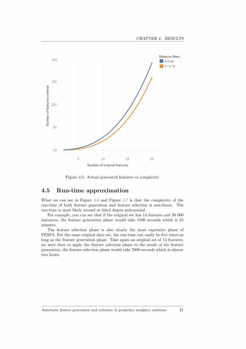
The complexity of all this combined is equal to the highest complexity amongthese equations which is O(n3). Take a look at Figure 4.5, where we havecalculated the number of features that would be created and have plotted itagainst the estimated complexity. Here we can see that the number of featuresthat will be created exceeds the number of features estimated by the complexityfunction.


CHAPTER 4. RESULTS

Figure 4.5: Actual generated features vs complexity

4.5 Run-time approximation

What we can see in Figure 4.6 and Figure 4.7 is that the complexity of therun-time of both feature generation and feature selection is non-linear. Therun-time is most likely second or third degree polynomial.

For example, you can see that if the original set has 14 features and 30 000instances, the feature generation phase would take 1500 seconds which is 25minutes.

The feature selection phase is also clearly the most expensive phase ofFESPA. For the same original data set, the run-time can easily be five times aslong as the feature generation phase. Take again an original set of 14 features,we were then to apply the feature selection phase to the result of the featuregeneration, the feature selection phase would take 7000 seconds which is almosttwo hours.


Figure 4.6: Run-time in seconds for feature generation

Figure 4.7: Run-time in seconds for feature selection after the feature generationphase, on a table with x original features

Chapter 5

Discussion

In this section, we will discuss implications of the results from Section 4, withregards to performance, operators and time versus accuracy. We will also discusssome ideas for future research.

5.1 Performance

As we can see in Figure 4.1, FESPA has a negative improvement over the originalperformance for just one data set. We can conclude from this that it is benefi-cial to apply FESPA, given the user has time. Obviously, applying FESPA, orany other feature generation and/or selection method, is more time-consumingthan taking the original feature set as the selected set. More on run-time inSection 5.4. Table 4.1 shows us that generally FESPA outperforms manual se-lection and Information Gain selection. It may not improve the performanceof more data sets than manual selection and Information Gain selection, butFESPA decreases the performance of only one data set whereas the other se-lection methods decrease the performance of all data sets where they do notimprove the performance.

When we compare Figure 4.1 to Figure 4.2(a), we can see that the featureselection phase of FESPA improves the performance if the input contains onlyoriginal features or also generated features.

When we compare Figure 4.1 to Figure 4.2(b), we see that applying only thefeature extraction phase of FESPA decreases the performance in most cases. Auser should always apply a selection method after the feature extraction phase ofFESPA, since this will improve the performance. Applying the selection methodof FESPA gives the greatest improvement and is even faster than the Inform-ation Gain method for data sets over 10 original features with all operatorsapplied.

I have found that most original features have as meta-feature indicator azero. Using a different check on line 8 of Algorithm 3 to give more originalfeatures a positive indicator can improve the performance of FESPA on originaldata sets.

Any small difference between FESPA and ExploreKit may also be due tothe difference of implementation, as ExploreKit was implemented in Java andFESPA was implemented in R. For such a relatively complex method, Java is a


CHAPTER 5. DISCUSSION

better choice than R for a programming language, as it is more object-oriented.In Java, it is easier to design custom objects that have their own parametersand methods. However, since R was already integrated in the Quintiq software,it was easier to implement FESPA in R.

5.2 Influence background collections

The hypothesis for the experiment from Section 4.2 was that a data set from acertain group would benefit most from background data sets from that group.However, the Diabetes data set is from the Medic group and in Figure 4.3 wecan see that the Medic group is not the best performing group. In Figure 4.4we can see that the best performing background data sets are in the Financeand Other group. Not only do the best performing background data sets notbelong to the Medic group, one of the data sets with the worst error score doesbelong to the Medic group. This tells us that there is no apparent correlationwithin a certain group of data sets.

5.3 Operators

In table 4.3, we can see which features are selected by FESPA. For five ofthe twelve data sets, FESPA could not find one or more features, generatedor original, that improve the original performance. As a result, FESPA thensimply returns the original feature set, see Algorithm 2. This ensures there isnever a decrease in performance.

The binary operators addition and multiplication are most present in theselected sets, whereas division is never selected. The group-by-then operatorswith aggregate functions Avg and Stdev are by far the most represented in theselected set.

For nearly half of the runs, FESPA actually selected features. Therefore,even though the binary division operator and the group-by-then Count, and Min

operators are not present in any selected set, we cannot confidently concludethat these operators will never be of importance for a data set.

5.4 Time versus accuracy

During this research, there has been one main theme. This was the problemof finding a balance between improving the accuracy and keeping the run-timewithin acceptable duration.

From a research point-of-view it is interesting to find the method and para-meter settings that optimize the performance. However, from a business point-of-view, the user-friendliness of the application has to be maintained. Thismeans that the run-time of the implemented methods cannot exceed a certainduration or the functionality would not be possible to use by day to day opera-tional tasks. The exact maximum acceptable duration depends on the applica-tion, the business operation this is applied to, the method, and the run-time ofalternative methods.

The bottleneck for FESPA is the group-by-then operators, since the com-plexity of these operators is n3, where n is the number of features, see Section


CHAPTER 5. DISCUSSION

4.4. We conclude that if results are needed in limited amount of time, it is bestto use only a few or none of the group-by-then operators. Since in our resultsthe most chosen group-by-then operators were Avg and Stdev, we recommendto choose these.

The results from Section 4.5 have lead to the decision to make the solutionmore adaptable by the user to make it fit their time frame. Therefore, in theimplementation, users can choose which operators to apply. If the user choosesless operators, then the run-time of both the feature generation phase and thefeature selection phase will decrease. This makes for a much more user-friendlyapplication.

5.5 Future work

The application can be made more user-configurable by enabling the user to notonly select which operators to use, but also which operators to use for whichfeatures. This will also help keep the resulting feature space of the feature gen-erator small. However, this will require a greater understanding of the methodthan the current implementation.

In future work, a functionality can be added that indicates how long thefeature generator or selector will run given the selected settings. Either bydefining a function with the possible settings as arguments, or as a predictiontask in itself.

Possibly, the application can be extended with a user-configurable classifiermethod. Currently, all classifiers implemented are decision trees. But, for ex-ample, if users want to use support vector machines instead of decision trees.The predictions of the meta-features will currently be based on the perform-ance of the background set features on a decision tree. However, whether acertain feature is influential can depend on the type of classifier used. Thereforeit is recommended to make the classifier method for the entire process user-configurable. Then the predictions of the meta-features will be based on theperformance of the background set features on support vector machines.


Bibliography

[1] Michael R Anderson, Dolan Antenucci, Victor Bittorf, Matthew Burgess,Michael J Cafarella, Arun Kumar, Feng Niu, Yongjoo Park, ChristopherRe, and Ce Zhang. Brainwash: A data system for feature engineering. InCIDR, 2013. 7

[2] L. Breiman, J. Friedman, R. Olshen, and C. Stone. Classification andRegression Trees. Wadsworth and Brooks, Monterey, CA, 1984. 4, 5, 6

[3] Edwin D De Jong and Tim Oates. A coevolutionary approach to represent-ation development. In Proc. of the ICML-2002 Workshop on Developmentof Representations, 2002. 7

[4] Rezarta Islamaj, Lise Getoor, and W John Wilbur. A feature generationalgorithm for sequences with application to splice-site prediction. FeatureSelection for Data Mining: Interfacing Machine Learning and Statistics,page 42, 2006. 2

[5] Uday Kamath, Kenneth De Jong, and Amarda Shehu. Effective automatedfeature construction and selection for classification of biological sequences.PloS one, 9(7):e99982, 2014. 5

[6] James Max Kanter and Kalyan Veeramachaneni. Deep feature synthesis:Towards automating data science endeavors. In Data Science and AdvancedAnalytics (DSAA), 2015. 36678 2015. IEEE International Conference on,pages 1–10. IEEE, 2015. 2

[7] Gilad Katz, Eui Chul Richard Shin, and Dawn Song. Explorekit: Auto-matic feature generation and selection. In Data Mining (ICDM), 2016IEEE 16th International Conference on, pages 979–984. IEEE, 2016. 6, 9

[8] Udayan Khurana, Deepak Turaga, Horst Samulowitz, and SrinivasanPartharathy. Cognito: Automated feature engineering for supervised learn-ing. In International Conference on Data Mining. IEEE, 2016. 7

[9] Hugh Leather, Edwin Bonilla, and Michael O’boyle. Automatic feature gen-eration for machine learning–based optimising compilation. ACM Trans-actions on Architecture and Code Optimization (TACO), 11(1):14, 2014.5

[10] Shaul Markovitch and Dan Rosenstein. Feature generation using generalconstructor functions. Machine Learning, 49(1):59–98, 2002. 2, 7


BIBLIOGRAPHY

[11] MuhammadArif Mohamad, Haswadi Hassan, Dewi Nasien, and HabibollahHaron. A review on feature extraction and feature selection for handwrittencharacter recognition. International Journal of Advanced Computer Science& Applications, 1(6):204–212, 2015. 2

[12] Hiroshi Motoda and Huan Liu. Feature selection, extraction and construc-tion. Communication of IICM (Institute of Information and ComputingMachinery, Taiwan) Vol, 5:67–72, 2002. 2

[13] Michael L Raymer, William F. Punch, Erik D Goodman, Leslie A Kuhn,and Anil K Jain. Dimensionality reduction using genetic algorithms. IEEEtransactions on evolutionary computation, 4(2):164–171, 2000. 2

[14] Olga Russakovsky, Jia Deng, Hao Su, Jonathan Krause, Sanjeev Satheesh,Sean Ma, Zhiheng Huang, Andrej Karpathy, Aditya Khosla, Michael Bern-stein, et al. Imagenet large scale visual recognition challenge. InternationalJournal of Computer Vision, 115(3):211–252, 2015. 5

[15] Ali Shadvar. Dimension reduction by mutual information feature extrac-tion. International Journal of Computer Science & Information Techno-logy, 4(3):13, 2012. 7


Appendix A

Overview data sets

In the table below, an overview is given of the data sets used in this research.

Data set #features #instances % numeric features

Contraceptive 9 1.473 66.6%CPU 12 8.192 100%

Credit 15 690 40%Delta elevators 6 9.517 100%

Diabetes 8 768 100%German credit 20 1.000 35%

Heart 13 270 46%Indian liver 10 585 90%

Mammography 6 11.183 100%Puma 8 8 8.192 100%Space 6 3.107 100%Wind 14 6.574 100%

Table A.1: Characteristics of used data sets


Appendix B

Algorithms pseudo-code

Algorithm 1: Feature generation

Data: datasetResult: dataset containing original and generated features

1 begin2 if doApplyUnary then3 dataset := applyUnaryOperators(dataset)4 end5 if doApplyBinary then6 binaryFeatures := applyBinaryOperators(dataset)7 end8 if doApplyGroupByThen then9 groupedFeatures := applyGBTOperators(dataset)

10 end11 return combine(dataset, binaryFeatures, groupedFeatures)

12 end


APPENDIX B. ALGORITHMS PSEUDO-CODE

Algorithm 2: FESPA - feature selection

Input: dataset, rankingThresholdOutput: dataset containing selected features

1 begin2 selectedSet := ∅3 features := dataset.GetFeatures()4 originalError := EvaluateOnLearner(features.GetOriginal())5 meta features := generateAllMetaFeatures(features)6 rankedFeatures := RankFeatures(features, meta features)7 PruneRankedFeatures(rankedFeatures, rankingThreshold)8 foreach feature in rankedFeatures do9 improvement := EvaluateOnLearner(selectedSet) -

EvaluateOnLearner(selectedSet ∪ feature)10 if improvement > thresholdfs then11 selectedSet := selectedSet ∪ feature12 end

13 end14 if selectedSet == ∅ then15 selectedSet := features.GetOriginal()16 end17 return selectedSet

18 end


APPENDIX B. ALGORITHMS PSEUDO-CODE

Algorithm 3: Building the background learner

Input: bg datasets: background datasetsOutput: dataset containing all meta-features of the background datasets

1 begin2 foreach bg dataset do3 originalFeatures := dataset.GetFeatures()4 originalError := EvaluateOnLearner(originalFeatures)5 foreach feature in originalFeatures do6 feature meta := generateFeatureMetaFeatures(feature)7 featureError := EvaluateOnLearner(feature)8 if featureError ≤ originalError - thresholdbg then9 feature meta.SetIndicator(1)

10 end11 else12 feature meta.SetIndicator(0)13 end

14 end15 dataset meta := generateDatasetMetaFeatures(bg dataset)16 dataset := generateFeatures(background dataset)17 foreach feature in dataset do18 feature meta := generateFeatureMetaFeatures(originalFeatures

∪ feature)19 featureError := EvaluateOnLearner(feature)20 if featureError ≤ originalError - thresholdbg then21 feature meta.SetIndicator(1)22 end23 else24 feature meta.SetIndicator(0)25 end

26 end

27 end28 return meta-features

29 end


Feature generation and selection - ru

Documents

Transcript of Feature generation and selection - ru