
DS2014: Feature selection in hierarchical feature spaces
37
1 Feature Selection in Hierarchical Feature Spaces Petar Ristoski, Heiko Paulheim 10/12/2014
-
Upload
petar-ristoski -
Category
Science
-
view
167 -
download
3
description
Feature selection is an important preprocessing step in data mining, which has an impact on both the runtime and the result quality of the subsequent processing steps. While there are many cases where hierarchic relations between features exist, most existing feature selection approaches are not capable of exploiting those relations. In this paper, we introduce a method for feature selection in hierarchical feature spaces. The method first eliminates redundant features along paths in the hierarchy, and further prunes the resulting feature set based on the features' relevance. We show that our method yields a good trade-off between feature space compression and classification accuracy, and outperforms both standard approaches as well as other approaches which also exploit hierarchies.
Transcript of DS2014: Feature selection in hierarchical feature spaces

1
Feature Selection inHierarchical Feature Spaces
Petar Ristoski, Heiko Paulheim10/12/2014

Motivation: Linked Open Data as Background
Knowledge
10/12/2014 2
• Linked Open Data is a method for publishing interlinked
datasets using machine interpretable semantics
• Started 2007
• A collection of ~1,000 datasets
– Various domains, e.g. general knowledge, government data, …
– Using semantic web standards (HTTP, RDF, SPARQL)
• Free of charge
• Machine processable
• Sophisticated tool stacks
Petar Ristoski, Heiko Paulheim

10/12/2014 3
Motivation: Linked Open Data as Background
Knowledge
Petar Ristoski, Heiko Paulheim
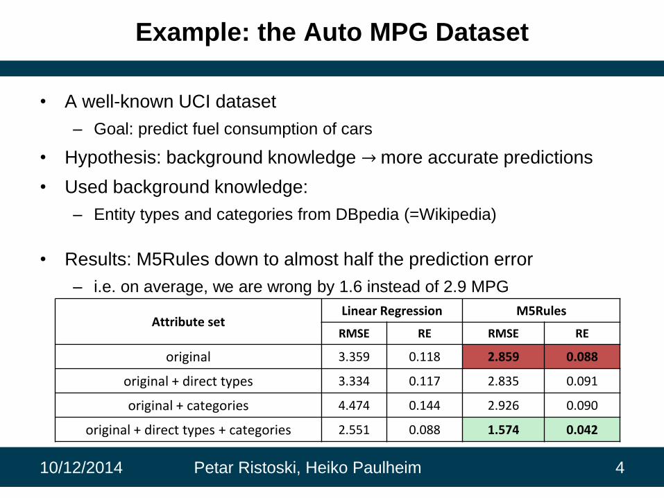
Example: the Auto MPG Dataset
• A well-known UCI dataset
– Goal: predict fuel consumption of cars
• Hypothesis: background knowledge → more accurate predictions
• Used background knowledge:
– Entity types and categories from DBpedia (=Wikipedia)
• Results: M5Rules down to almost half the prediction error
– i.e. on average, we are wrong by 1.6 instead of 2.9 MPG
10/12/2014 Petar Ristoski, Heiko Paulheim 4
Attribute setLinear Regression M5Rules
RMSE RE RMSE RE
original 3.359 0.118 2.859 0.088
original + direct types 3.334 0.117 2.835 0.091
original + categories 4.474 0.144 2.926 0.090
original + direct types + categories 2.551 0.088 1.574 0.042

Drawbacks
• The generated feature sets are rather large
– e.g. for dataset of 300 instances, it may generate up to 5,000 features
from one source
• Increase complexity and runtime
• Overfitting for too specific features
10/12/2014 5Petar Ristoski, Heiko Paulheim

Linked Open Data is Backed by Ontologies
10/12/2014 Petar Ristoski, Heiko Paulheim 6
LOD Graph Excerpt Ontology Excerpt

HIERARCHICAL FEATURE
SPACE
10/12/2014 Petar Ristoski, Heiko Paulheim 7

Problem Statement
• Each instance is an n-dimensional binary feature vector (v1,v2,…,vn),
where vi ∈ {0,1} for all 1≤ vi ≤n
• Feature space: V={v1,v2,…, vn}
• Hierarchic relation between two features vi and vj can be denoted as
vi < vj, where vi is more specific than vj
• For all hierarchical features, the following implication holds:
vi < vj→ (vi = 1 → vj = 1)
• Transitivity between hierarchical features exists:
vi < vj ˄ vj < vk→ vi < vk
• The problem of feature selection can be defined as finding a
projection of V to V’, where V’ ⊆ V and p(V’) ≥ p(V), where p is a
performance function:
𝑝: 𝑃 𝑉 → [0,1]
10/12/2014 Petar Ristoski, Heiko Paulheim 8
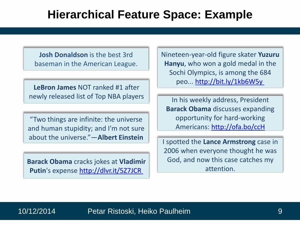
Hierarchical Feature Space: Example
10/12/2014 Petar Ristoski, Heiko Paulheim 9
Josh Donaldson is the best 3rd baseman in the American League.
LeBron James NOT ranked #1 after newly released list of Top NBA players
“Two things are infinite: the universe and human stupidity; and I'm not sure about the universe.”―Albert Einstein
In his weekly address, President Barack Obama discusses expanding
opportunity for hard-working Americans: http://ofa.bo/ccH
Nineteen-year-old figure skater YuzuruHanyu, who won a gold medal in the
Sochi Olympics, is among the 684 peo... http://bit.ly/1kb6W5y
Barack Obama cracks jokes at Vladimir Putin's expense http://dlvr.it/5Z7JCR
I spotted the Lance Armstrong case in 2006 when everyone thought he was
God, and now this case catches my attention.

10/12/2014 Petar Ristoski, Heiko Paulheim 10
Josh Donaldson is the best 3rd baseman in the American League.
LeBron James NOT ranked #1 after newly released list of Top NBA players
dbpedia:Josh_Donaldsondbpedia:LeBron_James
dbpedia-owl:Basketball_Player
dbpedia-owl:Baseball_Player
dbpedia-owl:Athlete
Hierarchical Feature Space: Example

Hierarchical Feature Space: Example
10/12/2014 Petar Ristoski, Heiko Paulheim 11
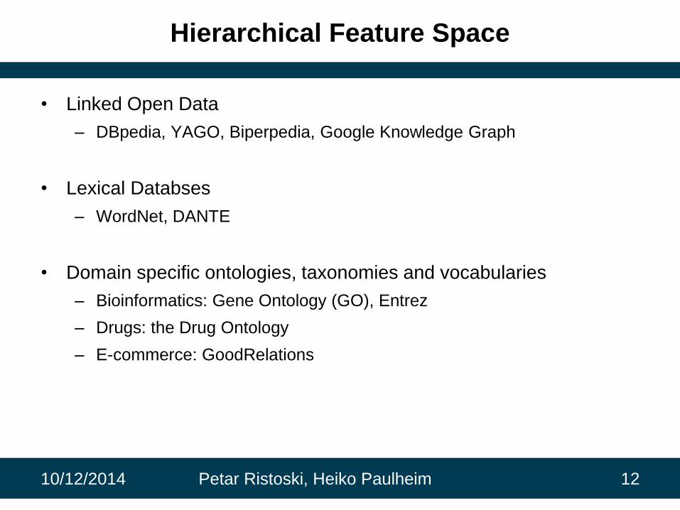
Hierarchical Feature Space
• Linked Open Data
– DBpedia, YAGO, Biperpedia, Google Knowledge Graph
• Lexical Databses
– WordNet, DANTE
• Domain specific ontologies, taxonomies and vocabularies
– Bioinformatics: Gene Ontology (GO), Entrez
– Drugs: the Drug Ontology
– E-commerce: GoodRelations
10/12/2014 Petar Ristoski, Heiko Paulheim 12

RELATED APPROACHES
10/12/2014 Petar Ristoski, Heiko Paulheim 13
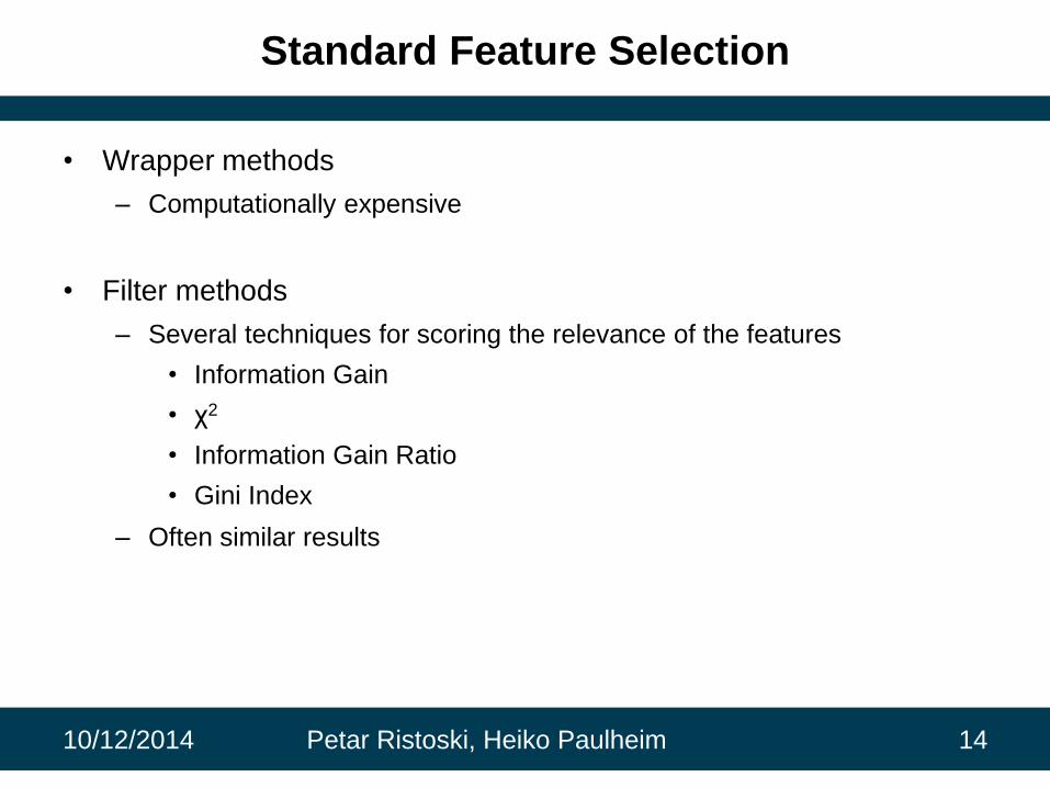
Standard Feature Selection
• Wrapper methods
– Computationally expensive
• Filter methods
– Several techniques for scoring the relevance of the features
• Information Gain
• χ2
• Information Gain Ratio
• Gini Index
– Often similar results
10/12/2014 Petar Ristoski, Heiko Paulheim 14

Optimal Feature Selection
10/12/2014 Petar Ristoski, Heiko Paulheim 15
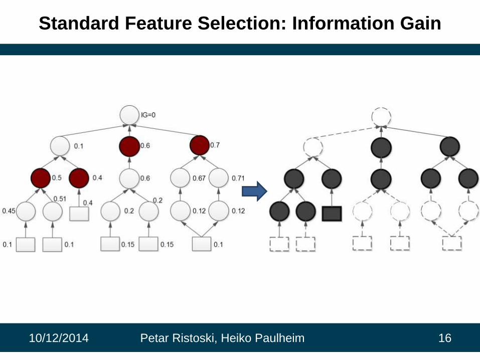
Standard Feature Selection: Information Gain
10/12/2014 Petar Ristoski, Heiko Paulheim 16
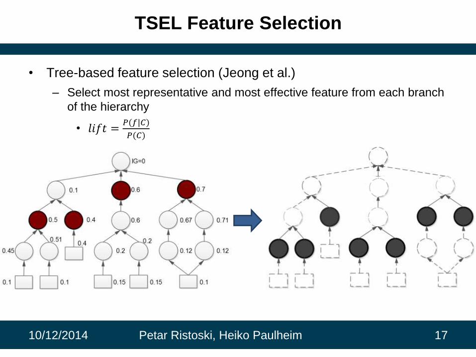
TSEL Feature Selection
• Tree-based feature selection (Jeong et al.)
– Select most representative and most effective feature from each branch
of the hierarchy
• 𝑙𝑖𝑓𝑡 =𝑃(𝑓|𝐶)
𝑃(𝐶)
10/12/2014 Petar Ristoski, Heiko Paulheim 17

Bottom-Up Hill-Climbing Feature Selection
• Bottom-up hill climbing search algorithm to find an optimal subset of
concepts for document representation (Wang et al.)
𝑓 = 1 +α − 𝑛
α∗ β ∗
𝑖∈𝐷𝐷𝑐𝑖 , 𝐷𝑐𝑖⊆ 𝐷𝐾𝑁𝑁𝑖 𝑎𝑛𝑑 β > 0
10/12/2014 Petar Ristoski, Heiko Paulheim 18

Greedy Top-Down Feature Selection
• Greedy based top-down search strategy for feature selection (Lu et al.)
– Select the most effective nodes from different levels of the hierarchy
10/12/2014 Petar Ristoski, Heiko Paulheim 19

PROPOSED APPROACH
10/12/2014 Petar Ristoski, Heiko Paulheim 20
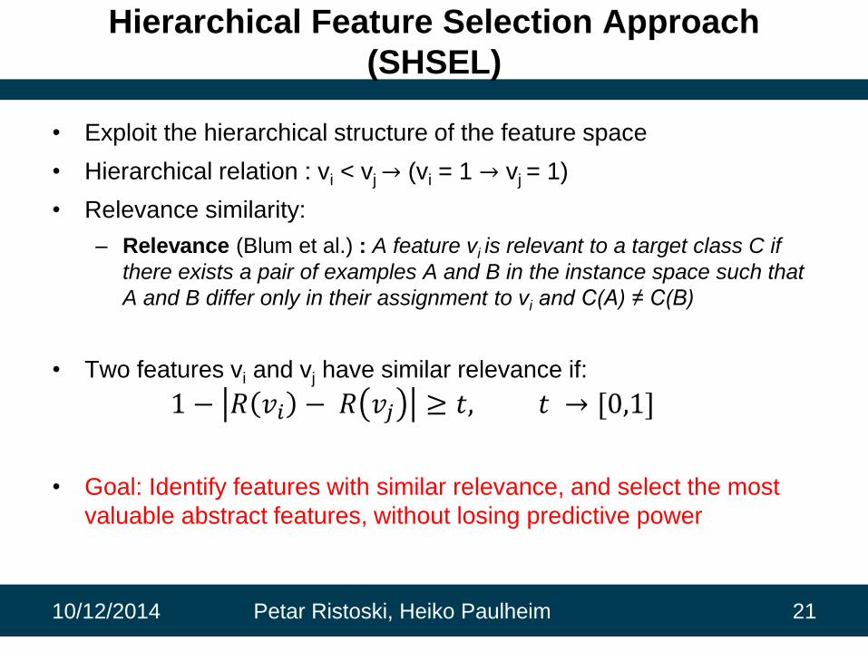
Hierarchical Feature Selection Approach
(SHSEL)
• Exploit the hierarchical structure of the feature space
• Hierarchical relation : vi < vj→ (vi = 1 → vj = 1)
• Relevance similarity:
– Relevance (Blum et al.) : A feature vi is relevant to a target class C if
there exists a pair of examples A and B in the instance space such that
A and B differ only in their assignment to vi and C(A) ≠ C(B)
• Two features vi and vj have similar relevance if:
1 − 𝑅 𝑣𝑖 − 𝑅 𝑣𝑗 ≥ 𝑡, 𝑡 → [0,1]
• Goal: Identify features with similar relevance, and select the most
valuable abstract features, without losing predictive power
10/12/2014 Petar Ristoski, Heiko Paulheim 21
Hierarchical Feature Selection Approach
(SHSEL)
• Initial Selection
– Identify and filter out ranges of nodes with similar relevance in each
branch of the hierarchy
• Pruning
– Select only the most relevant features from the previously reduced set
10/12/2014 Petar Ristoski, Heiko Paulheim 22
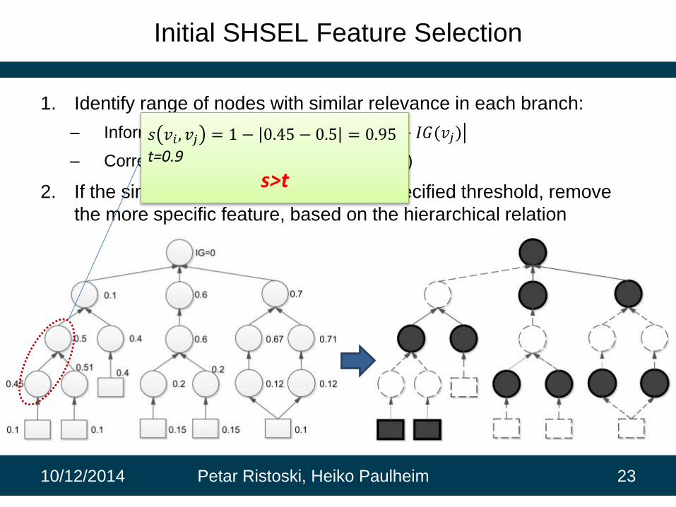
Initial SHSEL Feature Selection
1. Identify range of nodes with similar relevance in each branch:
– Information gain: 𝑠(𝑣𝑖 , 𝑣𝑗) = 1 − 𝐼𝐺 𝑣𝑖 − 𝐼𝐺(𝑣𝑗)
– Correlation: 𝑠(𝑣𝑖 , 𝑣𝑗) = 𝐶𝑜𝑟𝑟𝑒𝑙𝑎𝑡𝑖𝑜𝑛(𝑣𝑖 , 𝑣𝑗)
2. If the similarity is greater than a user specified threshold, remove
the more specific feature, based on the hierarchical relation
10/12/2014 Petar Ristoski, Heiko Paulheim 23
𝑠 𝑣𝑖 , 𝑣𝑗 = 1 − 0.45 − 0.5 = 0.95
t=0.9
s>t
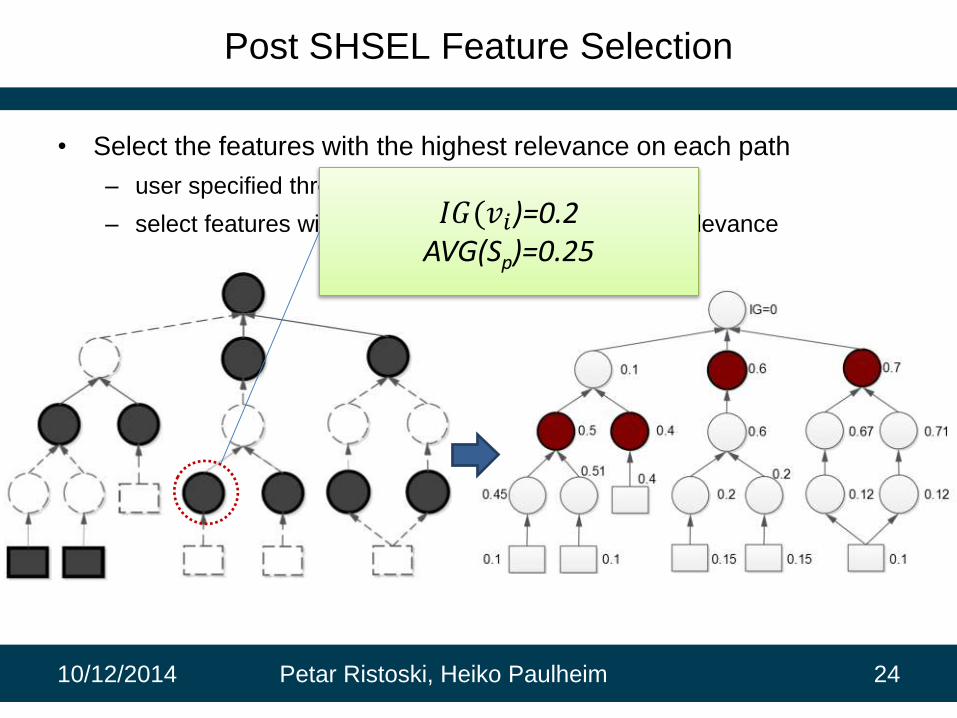
Post SHSEL Feature Selection
• Select the features with the highest relevance on each path
– user specified threshold
– select features with relevance above path average relevance
10/12/2014 Petar Ristoski, Heiko Paulheim 24
𝐼𝐺(𝑣𝑖)=0.2AVG(Sp)=0.25

EVALUATION
10/12/2014 Petar Ristoski, Heiko Paulheim 25
Evaluation
• We use 5 real-world datasets and 6 synthetically generated datasets
• Classification methods:
– Naïve Bayes
– k-Nearest Neighbors (k=3)
– Support Vector Machine (polynomial kernel function)
No parameter optimization
10/12/2014 Petar Ristoski, Heiko Paulheim 26

Evaluation: Real World Datasets
Name Features #Instances Class Labels #Features
Sports Tweets T DBpedia Direct Types 1,179 positive(523); negative(656) 4,082
Sports Tweets C DBpedia Categories 1,179 positive(523); negative(656) 10,883
Cities DBpedia Direct Types 212 high(67); medium(106); low(39) 727
NY Daily Headings DBpedia Direct Types 1,016 positive(580); negative(436) 5,145
StumbleUpon DMOZ Categories 3,020 positive(1,370); negative(1,650) 3,976
10/12/2014 Petar Ristoski, Heiko Paulheim 27
• Hierarchical features are generated from DBpedia (structured version of Wikipedia)
– The text is annotated with concepts using DBpedia Spotlight
• The feature generation is independent of the class labels, and it is unbiased towards any of the feature selection approaches

Evaluation: Synthetic Datasets
• Generate the middle layer using polynomial function
• Generate the hierarchy upwards and downwards following the
hierarchical feature implication and transitivity rule
• The depth and branching factor are controlled with parameters D
and B
10/12/2014 Petar Ristoski, Heiko Paulheim 28
Name #Instances Class Labels #Features
S-D2-B2 1,000 positive(500); negative(500) 1,201
S-D2-B5 1,000 positive(500); negative(500) 1,021
S-D2-B10 1,000 positive(500); negative(500) 961
S-D4-B2 1,000 positive(500); negative(500) 2,101
S-D4-B4 1,000 positive(500); negative(500) 1,741
S-D4-B10 1,000 positive(500); negative(500) 1,621
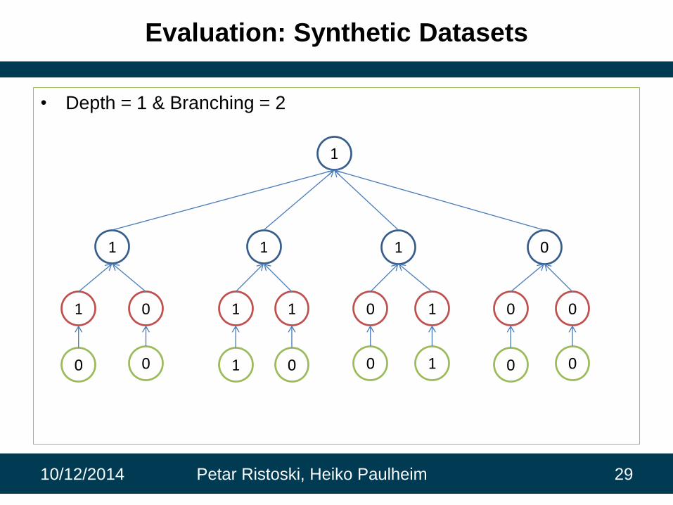
Evaluation: Synthetic Datasets
• Depth = 1 & Branching = 2
10/12/2014 Petar Ristoski, Heiko Paulheim 29
1 0 1 1 0 1 0 0
1 1 1 0
0
1
0 1 0 10 0 0

Evaluation: Synthetic Datasets
• Generate the middle layer using polynomial function
• Generate the hierarchy upwards and downwards following the
hierarchical feature implication and transitivity rule
• The depth and branching factor are controlled with parameters D
and B
10/12/2014 Petar Ristoski, Heiko Paulheim 30
Name #Instances Class Labels #Features
S-D2-B2 1,000 positive(500); negative(500) 1,201
S-D2-B5 1,000 positive(500); negative(500) 1,021
S-D2-B10 1,000 positive(500); negative(500) 961
S-D4-B2 1,000 positive(500); negative(500) 2,101
S-D4-B4 1,000 positive(500); negative(500) 1,741
S-D4-B10 1,000 positive(500); negative(500) 1,621

Evaluation: Approach
• Testing all approaches using two classification methods
– Naïve Bayes, KNN and SVM
• Metrics for performance evaluation
– Accuracy: Acc V′ =𝐶𝑜𝑟𝑟𝑒𝑐𝑡𝑙𝑦 𝐶𝑙𝑎𝑠𝑠𝑓𝑖𝑒𝑑 𝐼𝑛𝑠𝑡𝑎𝑛𝑐𝑒𝑠 (𝑉′)
𝑇𝑜𝑡𝑎𝑙 𝑁𝑢𝑚𝑏𝑒𝑟 𝑜𝑓 𝐼𝑛𝑠𝑡𝑎𝑛𝑐𝑒𝑠
– Feature Space Compression: 𝑐 𝑉′ = 1 −|𝑉′|
|𝑉|
– Harmonic Mean: 𝐻 = 2 ∗𝐴𝑐𝑐 𝑉′ ∗𝑐 𝑉′
𝐴𝑐𝑐 𝑉′ +𝑐 𝑉′
• Results calculated using stratified 10-fold cross validation
– Feature selection is performed inside each fold
• Parameter optimization for each feature selection strategy
10/12/2014 Petar Ristoski, Heiko Paulheim 31
0.00%
10.00%
20.00%
30.00%
40.00%
50.00%
60.00%
70.00%
80.00%
90.00%
100.00%
Relevance Similarity Threshold
Accuracy
Compression
H. Mean
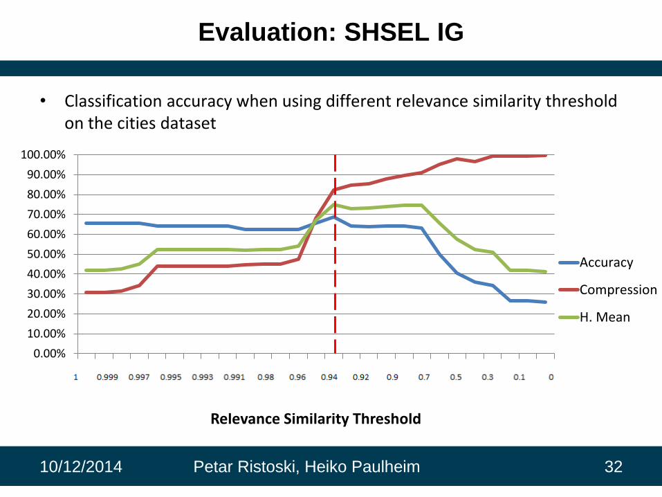
Evaluation: SHSEL IG
10/12/2014 Petar Ristoski, Heiko Paulheim 32
• Classification accuracy when using different relevance similarity threshold on the cities dataset

Evaluation: Classification Accuracy (NB)
10/12/2014 Petar Ristoski, Heiko Paulheim 33
0.00%
10.00%
20.00%
30.00%
40.00%
50.00%
60.00%
70.00%
80.00%
90.00%
100.00%
Sports Tweets T Sports Tweets C StumbleUpon Cities NY Daily Headings
original
initialSHSEL IG
initialSHSEL C
pruneSHSEL IG
pruneSHSEL C
SIG
SC
TSEL Lift
TSEL IG
HillClimbing
GreedyTopDown
0.00%
10.00%
20.00%
30.00%
40.00%
50.00%
60.00%
70.00%
80.00%
90.00%
100.00%
S_D2_B2 S_D2_B5 S_D2_B10 S_D4_B2 S_D4_B5 S_D4_B10
original
initialSHSEL IG
initialSHSEL C
pruneSHSEL IG
pruneSHSEL C
SIG
SC
TSEL Lift
TSEL IG
HillClimbing
GreedyTopDown
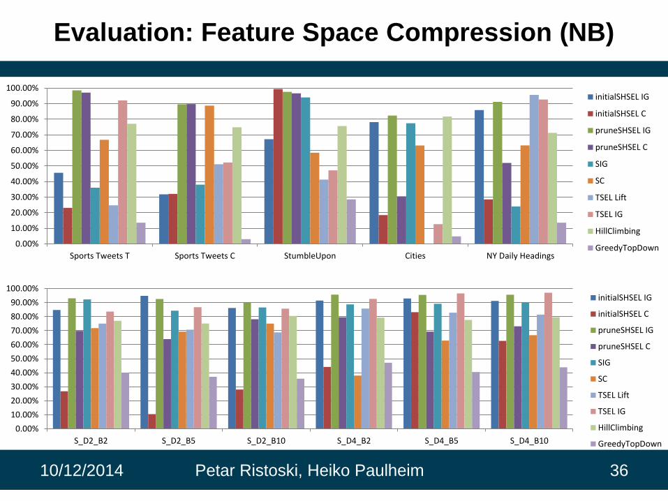
Evaluation: Feature Space Compression (NB)
10/12/2014 Petar Ristoski, Heiko Paulheim 36
0.00%
10.00%
20.00%
30.00%
40.00%
50.00%
60.00%
70.00%
80.00%
90.00%
100.00%
Sports Tweets T Sports Tweets C StumbleUpon Cities NY Daily Headings
initialSHSEL IG
initialSHSEL C
pruneSHSEL IG
pruneSHSEL C
SIG
SC
TSEL Lift
TSEL IG
HillClimbing
GreedyTopDown
0.00%
10.00%
20.00%
30.00%
40.00%
50.00%
60.00%
70.00%
80.00%
90.00%
100.00%
S_D2_B2 S_D2_B5 S_D2_B10 S_D4_B2 S_D4_B5 S_D4_B10
initialSHSEL IG
initialSHSEL C
pruneSHSEL IG
pruneSHSEL C
SIG
SC
TSEL Lift
TSEL IG
HillClimbing
GreedyTopDown

Evaluation: Harmonic Mean (NB)
10/12/2014 Petar Ristoski, Heiko Paulheim 39
0.00%
10.00%
20.00%
30.00%
40.00%
50.00%
60.00%
70.00%
80.00%
90.00%
100.00%
Sports Tweets T Sports Tweets C StumbleUpon Cities NY Daily Headings
initialSHSEL IG
initialSHSEL C
pruneSHSEL IG
pruneSHSEL C
SIG
SC
TSEL Lift
TSEL IG
HillClimbing
GreedyTopDown
0.00%
10.00%
20.00%
30.00%
40.00%
50.00%
60.00%
70.00%
80.00%
90.00%
100.00%
S_D2_B2 S_D2_B5 S_D2_B10 S_D4_B2 S_D4_B5 S_D4_B10
initialSHSEL IG
initialSHSEL C
pruneSHSEL IG
pruneSHSEL C
SIG
SC
TSEL Lift
TSEL IG
HillClimbing
GreedyTopDown

Conclusion & Outlook
10/12/2014 Petar Ristoski, Heiko Paulheim 43
• Contribution
– An approach that exploits hierarchies for feature selection in
combination with standard metrics
– The evaluation shows that the approach outperforms standard feature
selection techniques, and other approaches using hierarchies
• Future Work
– Conduct further experiments
• E.g. text mining, bioinformatics
– Feature Selection in unsupervised learning
• E.g. clustering, outlier detection
• Laplacian Score

44
Feature Selection inHierarchical Feature Spaces
Petar Ristoski, Heiko Paulheim10/12/2014


![Hierarchical Pyramid Diverse Attention Networks for Face ...openaccess.thecvf.com/content_CVPR_2020/papers/... · [40] generates local features on feature space by the ROI pooling.](https://static.fdocuments.in/doc/165x107/5f51c88060bee659b461e4f3/hierarchical-pyramid-diverse-attention-networks-for-face-40-generates-local.jpg)


